information to usersww2.che.ufl.edu/orazem/pdf-files/wojcik-phd-1997.pdfin the atlas of...
TRANSCRIPT

INFORMATION TO USERS
This manuscript has been reproduced from the microfilm master. UMI
films the text directly from the original or copy submitted. Thus, some
thesis and dissertation copies are in typewriter face, while others may be
from any type of computer printer.
The quality of this reproduction is dependent upon the quality of the
copy submitted. Broken or indistinct print, colored or poor quality
illustrations and photographs, print bleedthrough, substandard margins,
and improper alignment can adversely affect reproduction.
In the unlikely event that the author did not send UMI a complete
manuscript and there are missing pages, these will be noted. Also, if
unauthorized copyright material had to be removed, a note will indicate
the deletion.
Oversize materials (e.g., maps, drawings, charts) are reproduced by
sectioning the original, beginning at the upper left-hand corner and
continuing from left to right in equal sections with small overlaps. Each
original is also photographed in one exposure and is included in reduced
form at the back of the book.
Photographs included in the original manuscript have been reproduced
xerographically in this copy. Higher quality 6' x 9" black and white
photographic prints are available for any photographs or illustrations
appearing in this copy for an additional charge. Contact UMI directly to
order.
UMI A Bell & Howell Information Company
300 North Zeeb Road, Ann Arbor MI 48106-1346 USA 313n61-4700 S00/521-0600

THE ELECTROCHEMICAL BEHAVIOR OF COPPER AND COPPER NICKEL ALLOYS IN SYNTHETIC SEA
WATER
By
PAUL THOMAS WOJCIK
A DISSERTATION PRESENTED TO THE GRADUATE SCHOOL OF THE UNIVERSITY OF FLORIDA IN PARTIAL FULFILLMENT OF THE REQUIREMENTS FOR THE DEGREE OF DOCTOR OF PHILOSOPHY
UNIVERSITY OF FLORIDA
1997
UMI Number: 9802397
UMI Microform 9802397 Copyright 1997, by UMI Company. All rights reserved.
This microform edition is protected against unauthorized copying under Title 17, United States Code.
UMI 300 North Zeeb Road Ann Arbor, MI 48103

ACKNOWLEDGMENTS
The author wishes to express his gratitude to key individuals for their contribution
to this dissertation and to the enhancement of this learning experience. He \vould like to
thank Dr. Mark E. Orazem for his guidance, support and insightful suggestions. The
author would also like to thank members, both past and present, of the Electrochemical
Engineering Group at the University of Florida for their stimulating arguments and
intormative discussions. Oliver Moghissi and Steve Carson have been a great help on
topics of electrochemistry, and Pankaj Agarwal and Doug Reimer have been
indispensable in the areas of measurement models and computers respectively. His
mother and father receive a special thank you for supplying the advice, support of his
decisions, and encouragement which has made this educational experience truly
enjoyable.
II
TABLE OF CONTENTS
page
ACKNOWLEDGMENTS ·················································································· II
LIST OFT ABLES ····························································································· VI
LIST OF FIGURES ··························································································· VII
LIST OF SYMBOLS ························································································· XIV
ABSTRACT ······································································································ XVI
CHAPTER I INTRODUCTION ...................................................................... .
CHAPTER 2 BACKGROUND ........................................................................ 6
2.1 Copper Utility in Sea Water Environments ..................................... 6
2.2 Model Limitations .......................................................................... 7
2.2.1 Limitations ofthermodynamic information ........................ 7 2.2.2 Real system chemical characterization inadequacies .......... 8
2.2.3 Under-predicted reaction rates ........................................ 8 2.2.4 Chemical reaction times ................................................... 8
2.3 Thermodynamics ............................................................................ 8
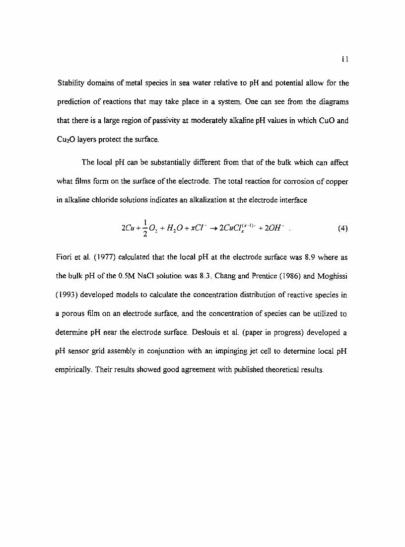
2.4 Corrosion in Alkaline Chloride Solutions ........................................ 18
2.5 Copper in Sea Water Environments ................................................ 20
2.6 Electrochemical Behavior of Copper in Aqueous Environments \Vith Flow 24 2.6.1 Erosion corrosion ............................................................ 24
2.6.2 Causes and indications ..................................................... 25
CHAPTER 3 ELECTROCHEMICAL TECHNIQUES .................................... 28
Ill

3.1 Large Signal Amplitude Measurement Techniques ........................... 29
3.2 Small Signal Amplitude Measurement Techniques........................... 29
3.3 Electrochemical Impedance Spectroscopy........................................ 30
CHAPTER 4 EXPERIMENTAL METHOD 36
4.1 Impinging Jet System 36
4.2 Sample and Solution Preparation ...................... ............. ........ 42 4.3 Experimental Procedure ........................................................ ...... 43
CHAPTER 5 VARIABLE AMPLITUDE GAL V ANOST A TIC ALLY MODULATED IMPEDANCE SPECTROSCOPY.................... 48
5.1 Variable-Amplitude Galvanostatic Modulation Algorithm ............... 55
5.2 Prediction ofthe Amplitude ofthe Current Perturbation .................. 56
5.3 Prediction ofthe Value for the Current Measuring Resistor ............. 58
5.4 Application to Corrosion Measurements........................................... 62
5.5 Comparison With Other Techniques ................................................ 64
5.6 Experimental Studies ......................................................................... 71
CHAPTER 6 RESULTS AND DISCUSSION ................................................. 76
6.1 The Measurement Model Approach ................................................ 78
6.2 Linear Sweep Voltammetry ............................................................ 79
6.3 Copper in Partially-Aerated Electrolyte: Part I ................................ 87
6.4 Copper in Partially-Aerated Electrolyte: Part 2 ................................ I 05 6.5 70130 Copper/Nickel Alloy in Aerated Electrolyte ........................... I II
6.6 Copper in Aerated Electrolyte ......................................................... I I 7
6. 7 X-ray Photoelectron Spectroscopy Analysis .................................... 128
6.8 Copper Rods in Synthetic Sea Water ............................................... 136
CHAPTER 7 COMPARISON WITH PAST RESULTS 147
CHAPTER 8 CONCLUSIONS ................................... ... . . . . ... .. ................... 155
CHAPTER 9 SUGGESTIONS FOR FUTURE WORK .................................... 158
iv
APPENDICES
A: ELECTROCHEMISTRY ................................................................. 161 8: TIME SUMMARIES .............................................. ......................... 165
REFERENCES .................................................................................................. 17 I
BIOGRAPHICAL SKETCH.............................................................................. I 79
v
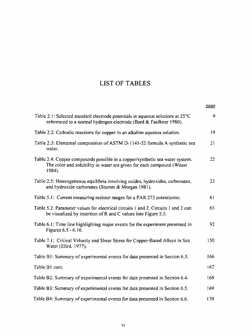
LIST OF TABLES
Table 2.1: Selected standard electrode potentials in aqueous solutions at 25°C 9 referenced to a normal hydrogen electrode (Bard & Faulkner I 980).
Table 2.2: Cathodic reactions for copper in an alkaline aqueous solution. 19
Table 2.3: Elemental composition of ASTM D- I 14 I -52 formula A synthetic sea 21 water.
Table 2.4: Copper compounds possible in a copper/synthetic sea water system. 22 The color and solubility in water are given for each compound (Weast I 984).
Table 2.5: Heterogeneous equilibria involving oxides, hydroxides, carbonates, 23 and hydroxide carbonates (Stumm & Morgan I 98 I).
Table 5. I : Current measuring resistor ranges for a PAR 2 73 potentiostat. 6 I
Table 5.2: Parameter values for electrical circuits I and 2. Circuits I and 2 can 65 be visualized by insertion ofR and C values into Figure 5.5.
Table 6. I: Time line highlighting major events for the experiment presented in 92 Figures 6.5 - 6. I 6.
Table 7. I: Critical Velocity and Shear Stress for Copper-Based Alloys in Sea I 50 Water (Efird, I 977).
Table B I: Summary of experimental events for data presented in Section 6.3. I 66
Table B I cont. I 67
Table B2: Summary of experimental events for data presented in Section 6.4. 168
Table B3: Summary of experimental events for data presented in Section 6.5. I 69
Table B4: Summary of experimental events for data presented in Section 6.6. I 70
VI

LIST OF FIGURES
Figure 2.1: Potential-pH equilibrium diagram for a copper I water system at 12 25°C. Solid substances under consideration are Cu, Cu20, and CuO. The numbers in this figure correspond to reactions given in the Atlas of Electrochemical Equilibria in Aqueous Solutions. A more detailed description of this figure is given in the reference (Pourbaix 1974 ).
Figure 2.2: Potential-pH equilibrium diagram for a copper I water system at 13 25°C. Solid substances under consideration are Cu, Cu20, and Cu(OH)2 (Pourbaix 1974 ). The numbers in this figure correspond to reactions given in the Atlas of Electrochemical Equilibria in Aqueous Solutions. A more detailed description ofthis figure is given in the reference (Pourbaix 1974).
Figure 2.3: Potential-pH equilibrium diagram for a copper I sea water system at 14 25°C. Solid substances under consideration are Cu, Cu20, CuCI, CuO, and Cu2(0H)3CI. The numbers in this figure correspond to reactions given in the reference which gives a detailed description ofthis figure (Bianchi & Longhi 1973 ).
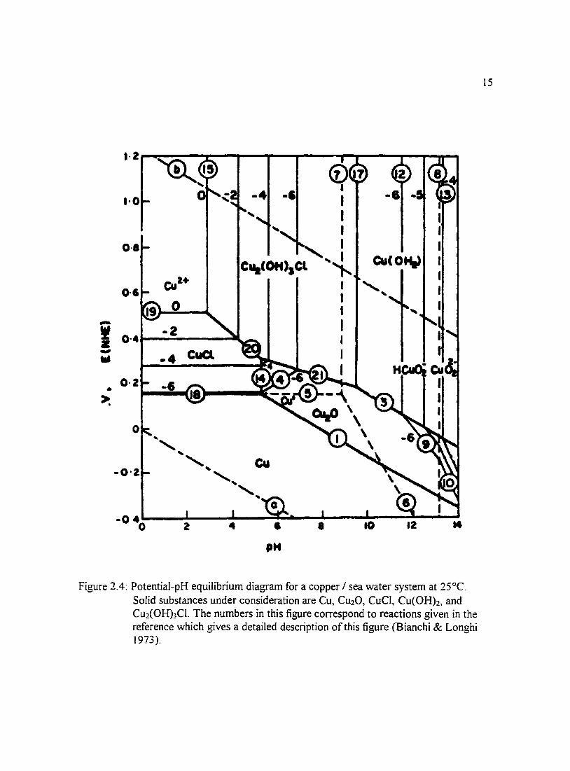
Figure 2.4: Potential-pH equilibrium diagram for a copper I sea water system at 15 25°C. Solid substances under consideration are Cu, Cu20. CuCI, Cu(OH)2, and Cu2(0H)3CI. The numbers in this figure correspond to reactions given in the reference which gives a detailed description of this figure (Bianchi & Longhi 1973).
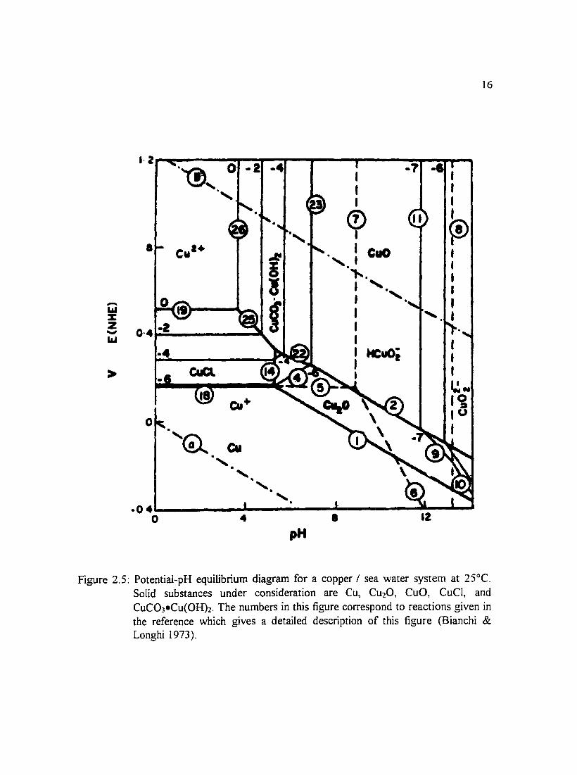
Figure 2.5: Potential-pH equilibrium diagram for a copper I sea water system at 16 25°C. Solid substances under consideration are Cu, Cu20, CuO, CuCJ, and CuC03·Cu(OH)2. The numbers in this figure correspond to reactions given in the reference which gives a detailed description ofthis figure (Bianchi & Longhi 1973 ).
VII
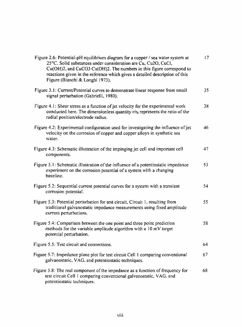
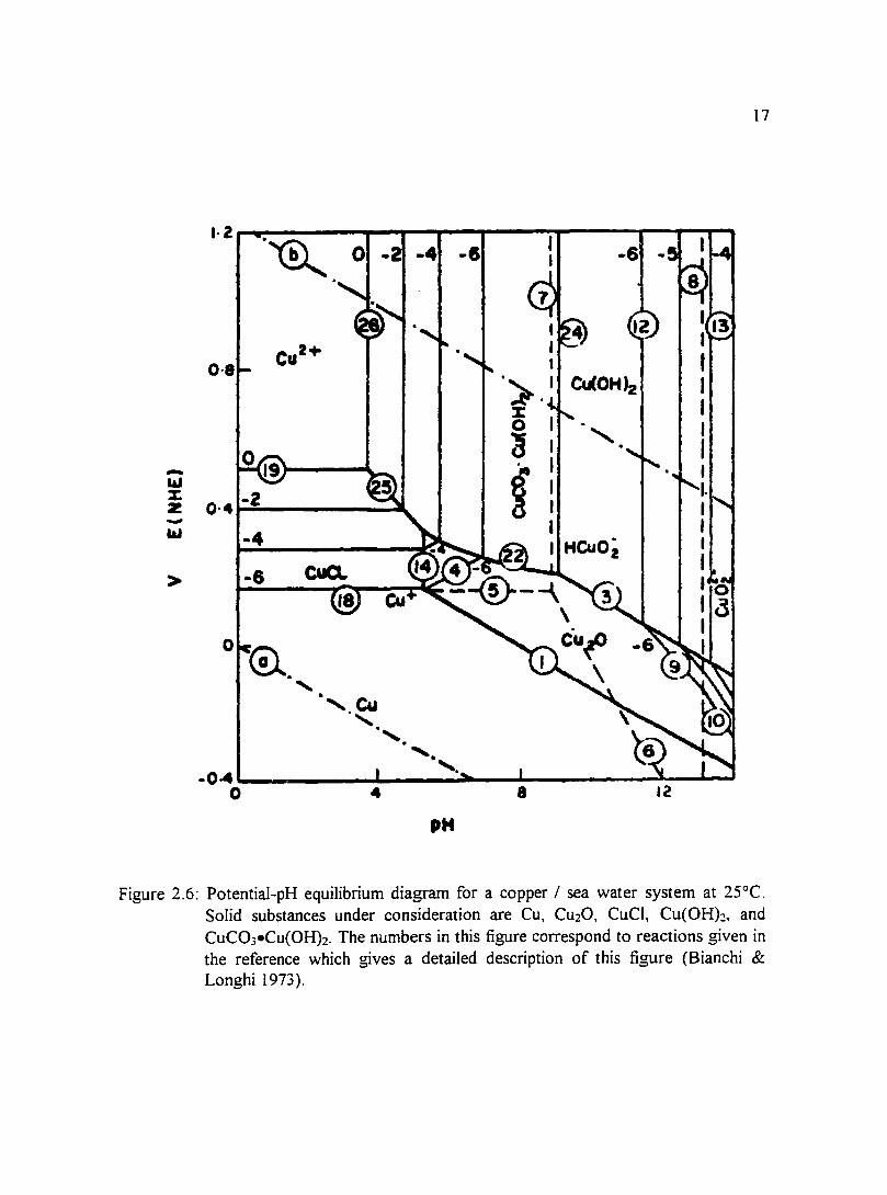
Figure 2.6: Potential-pH equilibrium diagram for a copper I sea water system at 17 25°C. Solid substances under consideration are Cu, Cu20, CuCI, Cu(OH)2, and CuC03·Cu(OH)2. The numbers in this figure correspond to reactions given in the reference which gives a detailed description of this Figure (Bianchi & Longhi 1973).
Figure 3.I: Current/Potential curves to demonstrate linear response from small 35 signal perturbation (Gabrielli, I980).
Figure 4.I: Shear stress as a function of jet velocity for the experimental work 38 conducted here. The dimensionless quantity r/r0 represents the ratio of the radial position/electrode radius.
Figure 4.2: Experimental configuration used for investigating the influence ofjet 46 velocity on the corrosion of copper and copper alloys in synthetic sea water.
Figure 4.3: Schematic illustration of the impinging jet cell and important cell components.
47
Figure 5.I: Schematic illustration of the influence of a potentiostatic impedance 53 experiment on the corrosion potential of a system with a changing baseline.
Figure 5.2: Sequential current potential curves for a system with a transient 54 corrosion potential.
Figure 5.3: Potential perturbation for test circuit, Circuit I, resulting from 55 traditional galvanostatic impedance measurements using fixed amplitude current perturbations.
Figure 5.4: Comparison between the one point and three point prediction 58 methods for the variable amplitude algorithm with a I 0 m V target potential perturbation.
Figure 5.5: Test circuit and connections. 64
Figure 5.7: Impedance plane plot for test circuit Cell I comparing conventional 67 galvanostatic, VAG, and potentiostatic techniques.
Figure 5.8: The real component of the impedance as a function of frequency for 68 test circuit Cell I comparing conventional galvanostatic, VAG, and potentiostatic techniques.
Vlll
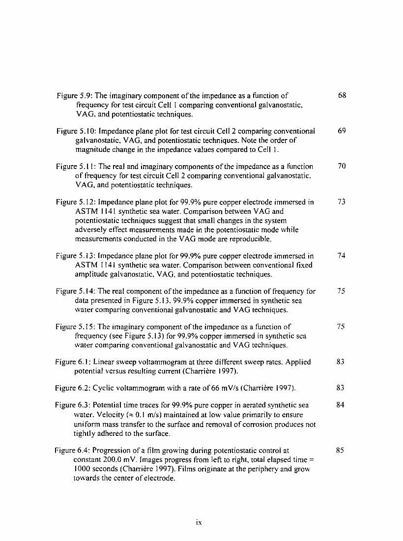
Figure 5.9: The imaginary component of the impedance as a function of 68 frequency for test circuit Cell l comparing conventional galvanostatic. VAG, and potentiostatic techniques.
Figure 5.10: Impedance plane plot for test circuit Cell 2 comparing conventional 69 galvanostatic, VAG, and potentiostatic techniques. Note the order of magnitude change in the impedance values compared to Cell l.
Figure 5.11: The real and imaginary components ofthe impedance as a tlmction 70 of frequency for test circuit Cell 2 comparing conventional galvanostatic. VAG, and potentiostatic techniques.
Figure 5.12: Impedance plane plot for 99.9% pure copper electrode immersed in 73 ASTM l 141 synthetic sea water. Comparison between VAG and potentiostatic techniques suggest that small changes in the system adversely effect measurements made in the potentiostatic mode while measurements conducted in the VAG mode are reproducible.
Figure 5.13: Impedance plane plot for 99.9% pure copper electrode immersed in 74 ASTM l 141 synthetic sea water. Comparison between conventional fixed amplitude galvanostatic. VAG, and potentiostatic techniques.
Figure 5.14: The real component ofthe impedance as a function of frequency for 75 data presented in Figure 5.13. 99.9% copper immersed in synthetic sea water comparing conventional galvanostatic and VAG techniques.
Figure 5.15: The imaginary component ofthe impedance as a function of 75 frequency (see Figure 5.13) for 99.9% copper immersed in synthetic sea water comparing conventional galvanostatic and VAG techniques.
Figure 6.1: Linear sweep voltammogram at three different sweep rates. Applied 83 potential versus resulting current (Charriere 1997).
Figure 6.2: Cyclic voltammogram with a rate of66 mV/s (Charriere I 997). 83
Figure 6.3: Potential time traces for 99.9% pure copper in aerated synthetic sea 84 water. Velocity(:::: 0. I m/s) maintained at low value primarily to ensure uniform mass transfer to the surface and removal of corrosion produces not tightly adhered to the surface.
Figure 6.4: Progression of a film growing during potentiostatic control at 85 constant 200.0 m V. Images progress from left to right, total elapsed time =
I 000 seconds (Charriere 1997). Films originate at the periphery and grmv to\vards the center of electrode.
IX
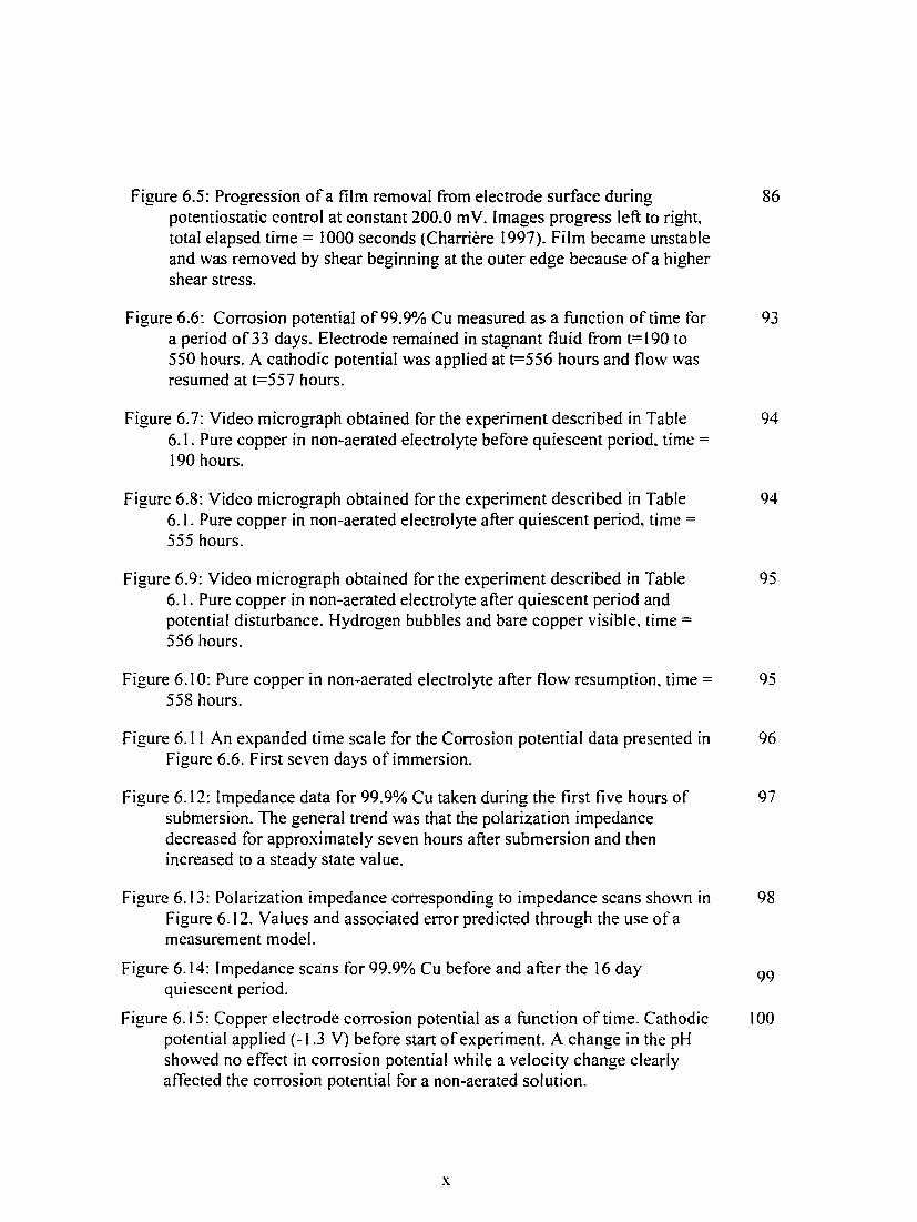
Figure 6.5: Progression of a film removal from electrode surface during potentiostatic control at constant 200.0 m V. Images progress left to right. total elapsed time= I 000 seconds (Charriere 1997). Film became unstable and was removed by shear beginning at the outer edge because of a higher shear stress.
Figure 6.6: Corrosion potential of99.9% Cu measured as a function oftime for a period of33 days. Electrode remained in stagnant fluid from t=l90 to 550 hours. A cathodic potential was applied at t=556 hours and flow was resumed at t=557 hours.
Figure 6. 7: Video micrograph obtained for the experiment described in Table 6.1. Pure copper in non-aerated electrolyte before quiescent period. time = 190 hours.
Figure 6.8: Video micrograph obtained for the experiment described in Table 6.1. Pure copper in non-aerated electrolyte after quiescent period. time = 555 hours.
Figure 6.9: Video micrograph obtained for the experiment described in Table 6.1. Pure copper in non-aerated electrolyte after quiescent period and potential disturbance. Hydrogen bubbles and bare copper visible. time= 556 hours.
Figure 6.10: Pure copper in non-aerated electrolyte after flow resumption. time= 558 hours.
Figure 6.1 I An expanded time scale for the Corrosion potential data presented in Figure 6.6. First seven days of immersion.
Figure 6.12: Impedance data for 99.9% Cu taken during the first five hours of submersion. The general trend was that the polarization impedance decreased for approximately seven hours after submersion and then increased to a steady state value.
Figure 6.13: Polarization impedance corresponding to impedance scans shown in Figure 6.12. Values and associated error predicted through the use of a measurement model.
Figure 6.14: Impedance scans for 99.9% Cu before and after the 16 day quiescent period.
Figure 6.15: Copper electrode corrosion potential as a function of time. Cathodic potential applied ( -1.3 V) before start of experiment. A change in the pH showed no effect in corrosion potential while a velocity change clearly affected the corrosion potential for a non-aerated solution.
X
86
93
94
94
95
95
96
97
98
99
100

Figure 6.I6: Impedance data collected for 99.9% Cu over the course of23 I lO I hours corresponding to the corrosion potential data in Figure 6.I5.
Figure 6.I7: Polarization impedance encompassing impedance scans shown in l 02 Figure 6.16. Values and associated error were predicted through the use of a measurement model.
Figure 6.I8: Video micrograph obtained for the experiment described in Table l 03 6.I. Pure copper in non-aerated electrolyte immediately after submersion. time= 0 hours. Polished state.
Figure 6.I9: Video micrograph obtained for the experiment described in Table l 03 6.I. Pure copper in non-aerated electrolyte at time = I69 hours.
Figure 6.20: Video micrograph obtained for the experiment described in Table I 04 6.I. Pure copper in non-aerated electrolyte at time = 67I hours.
Figure 6.2I: Video micrograph obtained for the experiment described in Table l 04 6.I. Pure copper in non-aerated electrolyte at time = 8I4 hours.
Figure 6.22: Corrosion potential as a function oftime for a 99.9% pure copper I08 electrode in non aerated ASTM I I4I electrolyte. Change in the corrosion potential due to velocity increase is evident.
Figure 6.23: Impedance collected on 99.9% copper over a period of I44 hours. I09 The solution was not aerated and the etTect of a velocity change from 2.0 to 6.2 m/s is observable.
Figure 6.24: Nyquist plot for VAG experiments at different target amplitudes for l I 0 99.9% pure copper in non-aerated synthetic sea water. Effect of all amplitudes below 50.0 mV are reversible. An amplitude of50.0mV dramatically and irreversibly changes the surface ofthe electrode.
Figure 6.25: Corrosion potential (SCE) data collected on 70/30 copper/nickel II3 over a period of 288 hours. The solution was aerated with C02 scrubbed air and the effect of a velocity change from 2.0 to 6.0 m/s is observable.
Figure 6.26: Impedance plane plot of several impedance spectra collected on a I I4 70130 copper/nickel alloy electrode with C02 scrubbed aeration over the course of II days. The susceptibility ofthe film to disturbance and measurement procedure is evident from the sporadic increase and decrease ofthe impedance values.
Figure 6.27: Impedance data collected on 70/30 copper/nickel corresponding to II5 corrosion potential data in Figure 6.25. The solution was aerated with C02
scrubbed air and a slight effect of a velocity change from 2.0 to 6.0 m/s is observable.
XI

Figure 6.28: Polarization impedance predicted by the measurement model for I 16 70/30 copper nickel alloy in synthetic sea water.
Figure 6.29: Corrosion potential measured of copper as a function of time for 120 well aerated synthetic sea water electrolyte. A negligible effect of velocity is seen.
Figure 6.30: lmpedance plane plot for copper electrode in well aerated sea water 121 before and after velocity change from 1.0 to 2.0 mls.
Figure 6.31: lmpedance plane plot for copper electrode in well aerated sea water 122 before and after velocity change !Tom 2.0 to 6.0 m/s.
Figure 6.32: lmpedance plane plot for copper electrode in \Veil aerated sea \Vater 123 over the course of three velocity changes.
Figure 6.33: Polarization tor aerated copper synthetic sea water system. Values 124 and associated error predicted through the use of a measurement model.
Figure 6.34: Corrosion potential data for the tirst 24 hours for data presented in 125 Figure 6.29.
Figure 6.35: lmpedance plane plot for copper electrode in well aerated sea water 126 for the first 24 hours of submersion. Jet velocity = 1.0 m/s.
Figure 6.36: Predicted polarization impedance for data displayed in Figure 6.35. 127 Values predicted using the measurement model technique.
Figure 6.37: XPS and SEM data for copper electrode immersed in partially 131 aerated sea water. Magnification for SEM micrograph= 2000X.
Figure 6.38: XPS data for copper electrode after exposure in partially aerated sea 132 water. Analysis for entire electrode surface.
Figure 6.39: XPS and SEM data for copper electrode after exposure in aerated 133 sea water. Magnification for SEM micrograph = 250X.
Figure 6.40: XPS and SEM data for copper electrode after exposure in aerated 134 sea water. Magnification for SEM micrograph= 250X.
Figure 6.41: XPS and SEM data for copper electrode after exposure in aerated 135 sea water. Magnification for SEM micrograph= 750X.
Figure 6.42: Trailing edge of copper electrode. Oxide film visible near center of 139 downstream portion of the electrode. The direction of flow of the electrolyte is out from the page.
XII
Figure 6.43: Copper electrode with non-uniform oxide film. [mage shows areas 140 where the film has adhered to the electrode. The direction of flow of the electrolyte is out trom the page.
Figure 6.44: Edge of copper electrode normal to electrolyte flow. Transition 141 phase evident at white boundary. Green film visible at left of image which was the trailing edge of the electrode. The direction of flow of the ... ... electrolyte is to the left.
Figure 6.45: Copper electrode at the solution air interface. Flow pattern indicated 142 by white band on electrode surface which indicates a velocity reduction near the solution/air interface. The direction of flow of the electrolyte is to the left.
Figure 6.46 : Precipitate collected from bottom of recirculation beaker. Blue- 143 green in color, precipitate was collected in a pipette ..
Figure 6.47: Precipitate on sample paper, wet. 144
Figure 6.48 : Precipitate on sample paper after air drying. 145
Figure 6.49: VAG impedance scans conducted on each rod. Three consecutive 146 scans were collected on each rod and a general downward trend is seen for both cases. Also plotted is a preliminary potentiostatic scan used in determining experimental parameters.
Figure 7.1: Cleaned images used to determine critical shear by Efird ( 1977). 151
Figure 7.2 Shear stress as a function of jet velocity. Curves indicate 152 dimensionless position on the electrode. Horizontal lines represent reported values for critical shear for copper and 70/30 copper nickel (Efird. 1977).
Figure 7.3: Shear stress as a function of jet velocity. Curves indicate 153 dimensionless position on the electrode. Horizontal lines represent reported values for critical shear for copper and 70/30 copper nickel (Efird. 1977).
Figure 7.4: Image of pure copper electrode in aerated sea water from experiment 154 discussed in section 6.6. Velocity had been held constant at 2.0 m/s for 44 hours when image was obtained. No indications of enhanced corrosion (H26.tif).
xiii

LIST OF SYMBOLS
a hydrodynamic constant, s-1
A electrode area, cm2
C; concentration of species !, mol/cm3
c capacitance, ~-tf
d diameter, em
D diffusivity, cm2/s
E potential. V
Es electron's original binding energy, eV
f frequency, Hz
F Faraday's constant, 96,487 C/equiv
H height, em
i current density, mA/cm2
current, rnA
Keq equilibrium constant
q double layer charge. C/cm2
R resistance, Q
Rp polarization resistance, n
R universal gas constant 8.314 J/moi/K
T temperature, K
v velocity. m/s
Zr real impedance. n zj imaginary impedance, n
a a apparent transfer coefficient, anodic
ac apparent transfer coefficient, cathodic
xiv
p density. g/cm3
~ viscosity, cP
v kinematic viscosity, cm2/s
(!) frequency, rad/s
cf> potential, V
<P stream function
ll dimensionless axial position .,
t shear stress, N/m-
hv X-ray energy
XV
Abstract of Dissertation Presented to the Graduate School of the University of Florida in Partial Fulfillment of the Requirements for the Degree of Doctor of Philosophy
THE ELECTROCHEMICAL BEHAVIOR OF COPPER AND COPPER NICKEL ALLOYS
IN SYNTHETIC SEA WATER
By
Paul Thomas Wojcik
August, 1997
Chairman: Mark E. Orazem Major Department: Chemical Engineering
The goal of this work was to investigate the mechanism(s) of erosion-corrosion of
copper and copper alloys in high velocity synthetic sea water environments. An
impinging jet cell was designed to provide a platform where specific modes of enhanced
corrosion could be isolated. A novel galvanostatic impedance technique was developed to
collect impedance spectra without disrupting the temporal evolution of the system. A
measurement model technique was applied to the impedance spectra to predict the
polarization impedance and filter inconsistent data. The effect of velocity. pH, aeration.
and applied potentials on the corrosion behavior of copper and copper alloys was
investigated using electrochemical impedance spectroscopy, corrosion potential
monitoring, and analysis of digital image captures.
A video microscope was used to provide a visual record of the electrode surface
which could be used to determine shear-induced enhance corrosion. Results were
XVI

compared with reported values and mechanisms for enhanced corrosion of previously
reported work were proposed.
xvii

CHAPTER 1 INTRODUCTION
The object of this work was to investigate the phenomenon of enhanced corrosion
of copper and copper nickel alloys in high-velocity sea water environments. This work
was motivated by conflicting reports in the literature describing the mechanisms of
enhanced corrosion in high velocity environments and the conditions necessary for
enhanced corrosion to occur.
In 1977, K.D. Efird investigated copper and copper based alloys in high velocity
sea water environments. Efird conducted experiments in a channel flow apparatus where
samples were exposed to fresh sea water procured from the Atlantic Ocean off the coast
of the Francis L. LaQue Corrosion Laboratory, Wrightsville Beach, North Carolina. The
samples were exposed for thirty days at different velocities after which the samples were
analyzed. Efird observed enhanced corrosion in the form of pits and waves on the coupon
surface for velocities above a certain value. A shear stress corresponding with the
empirically determined velocity was mathematically calculated and was referred to as the
critical shear for the material tested. Efird concluded that copper (or copper alloys)
subjected to shear values above the critical shear would exhibit enhanced corrosion. Efird
also concluded that the mechanism responsible for the enhanced corrosion was the
mechanical removal of a protective oxide film on the surface of the sample.
2
C. B. Diem ( 1990) conducted work on copper electrodes in aerated 0.62 M sodium
chloride solutions with pH values of 8.5 and 9.5 to investigate the effect of shear stress on
the anodic dissolution of copper. An axisymmetric impinging jet apparatus was utilized in
conjunction with a scanning ellipsometer. The impinging jet configuration was chosen to
ensure uniform mass transfer to the electrode surface and shear stress proportional to
radial position. Experiments were conducted at velocities above values corresponding to
the critical shear value for copper reported by Efird and no enhanced corrosion was
observed. Diem concluded that erosion-corrosion of copper in alkaline chloride solutions
is not caused by a shear-induced removal of protective films. Diem suggested non-uniform
mass transfer and particle impingement as possible contributors to the enhanced corrosion
observed by Efird. A direct comparison between the work of Diem and Efird was not
possible due to differences in the aqueous environments studied. The work conducted by
Diem involved short term experiments on the order of hours, whereas, Efird's experiments
were conducted over a period of thirty days.
For this work an impinging jet cell was designed and built \vith several
improvements to better investigate the free corrosion of copper and copper nickel alloys in
high-velocity synthetic sea water environments. The goals of this work were to
• determine the mechanism for enhanced corrosion of copper and copper nickel
alloys in high velocity environments
• determine if hydrodynamic shear can remove protective films.
The importance of this work lies in the fact that copper is a popular material for
use in marine environments. Key features contributing to the widespread use of copper are
..., _,
desirable material characteristics and cost effectiveness. The approach to this problem
involved design of an experimental system to investigate specific causes of enhanced
corrosion in high velocity environments. Electrochemical techniques were applied to
monitor the reactivity and state of the electrode surface (Syrett & Macdonald 1979).
Corrosion potential measurements and impedance spectroscopy were used to monitor
electrochemical properties of the electrode surface, and video microscopy was used to
observe the surface and to record events as a function of time.
Copper and copper alloys are well suited for marine applications. Copper has a
high thermodynamic stability and forms a protective oxide film, which can decrease or
eliminate corrosion. The world's oceans are teaming with living organisms which can
adhere to exposed surfaces and alter the chemical reactions occurring on the surface, in
turn, affecting the rate of corrosion. Copper is toxic to many organisms and, this, reduces
the risk of microbiologically influenced corrosion (Gilbert 1982).
Unexpectedly high corrosion rates have been reported m high velocity
environments which are common in marine heat exchangers and in regions of turbulence
around the periphery of marine screws (LaQue 1975, Efird 1977). There are many
methods available for inhibiting corrosion in copper systems although in the vicinity of
marine screws or heat exchangers, these methods may not be effective or practical
(Goodman 1987). Increased mass transfer of corrosive species to the surface and
corrosion products away from the surface (Diem & Orazem 1994), shear induced removal
of a protective film, cavitation causing disruption of the film and surface damage (Wood et
al. 1990a), as well as impingement of particles onto the surface resulting in protective film
removal, have all been suggested as possible causes of the increased corrosion rate

4
(Copson 1960, Dawson et al. 1990, Heitz 1991, Sethi & Wright 1991, Somerscales &
Sanatgar 1991 ). In many cases the effects of erosion of the film and corrosion act
synergistically, i.e., the total effect is greater than the sum of the individual effects.
A novel approach to conducting galvanostatically controlled impedance
experiments was developed during this work (Wojcik et al. 1996, Wojcik & Orazem
1997a, Wojcik & Orazem l997c). The utility ofthis modified galvanostatic technique was
to non-invasively investigate actively corroding systems where the baseline corrosion
potential changes with time. The development of the variable amplitude galvanostatic
(VAG) technique addressed problems inherent with both potentiostatic and conventional
galvanostatic regulation. The VAG technique utilizes previously acquired impedance data
to predict the impedance value for the next frequency. The predicted impedance value is
used to determine an optimum value for the current perturbation and current measuring
resistor for the next measurement. This predictive technique ensures acceptable signal to
noise ratio as well as a linear signal response.
Background information including electrochemical processes, thermodynamics of
copper, film formation and enhanced corrosion in high velocity environments are discussed
in Chapter 2. The theory behind electrochemical impedance spectroscopy, different
methods of conducting impedance experiments, and examples of applications are
presented in Chapter 3. The cell design and instrumentation used to conduct experiments
and collect data is described in Chapter 4. The reason the impinging jet configuration was
chosen over other cell designs is also explained in this chapter. A description of the
procedures used to conduct experiments is given in Chapter 4 as well as the preparation
techniques used for samples and solutions. The technique described in Chapter 5

5
incorporates the positive aspects of both potentiostatic and conventional galvanostatic
regulation. Comparisons are made between the variable amplitude galvanostatic technique
and other commonly applied techniques for a variety of test systems.
Discussion and results are the topics of Chapter 6 where a brief explanation of the
measurement model technique is given. Corrosion potential analysis, impedance spectra
analysis, x-ray photoelectron spectroscopy, scanning electron microscopy, linear sweep
voltarnmetry and image analysis are covered in this chapter. Comparisons of the results
obtained in this work and results previously reported are presented in Chapter 7.
Conclusions drawn from this work are discussed in Chapter 8 and recommendations for
future work are discussed in Chapter 9.
CHAPTER2 BACKGROUND
The utility of copper for use in sea water environments and the limitations of
models are discussed in Chapter 2. Issues of the thermodynamics of copper are
presented, and the corrosion of copper in alkaline chloride solutions, sea water, and
environments with flow is discussed in this chapter.
2.1 Copper Utility in Sea Water Environments
Copper and copper alloys have a long history of use in marine applications and
other corrosive environments. Recent developments of high performance materials which
equal or exceed the desired characteristics of copper have not reduced the wide use of
copper and copper alloys in industrial applications. The longevity of copper and copper
alloys can be attributed to economics and a combination of desirable material
characteristics.
Copper is relatively inexpensive when compared to materials with comparable
corrosion resistant properties e.g. titanium. Copper is found in a natural state and is also
present in a number of ores including cuprite, malachite, azurite, chalcopyrite, and bornite.
Copper ores are currently the primary source for refined copper. Copper is extracted from
the ore by means of smelting, leaching, and electrolysis. The thermal conductivity of pure
6
7
copper at 473 K is 389 W/m•K compared to iron, 304 stainless steal, pure nickel, and
titanium with values of 66, 18, 74, and 20 W/m•K respectively (White 1984). Copper is
second only to silver in electrical conductivity (Weast 1984). The machinability of copper
and copper alloys combined with other physical properties make these metals excellent
materials for a wide variety of applications including use in heat exchangers and other
complicated parts.
2.2 Model Limitations
Discrepancies can exist between results predicted by an equilibrium model and
empirically determined real system parameters. The goal of modeling is to closely
approximate the real system of interest. There are several reasons for discrepancies
between model approximations and real system. Models usually require approximations
and/or dismissal of certain parameters that are not well understood or are believed to be
negligible. This can lead to errors in the model's predictive capabilities. One hopes to be
able to describe a real system in terms of a first approximation with an equilibrium model.
A brief description of sources of errors in equilibrium models is given as follows.
2.2.1 Limitations of thermodynamic information
The lack of consideration of important species in solution or solid phases is an
example of a source of error. The Pourbaix diagrams, while valuable, may not consider all
possible species. The thermodynamic data for the species considered may be incorrect or
8
inadequate. Temperature and pressure corrections may not be accurate and can vary
dramatically in natural sea waters.
2.2.2 Real system chemical characterization inadequacies
Analytical data for species may not be adequate to determine the physical or
chemical forms (i.e. oxidized/reduced, suspended/dissolved) of chemical elements m
complex real systems where interactions with other species are present.
2.2.3 Under-predicted reaction rates
An equilibrium state in a real system may be achieved slowly due to rates of some
chemical reactions.
2.2.4 Chemical reaction times
For irreversible reactions, no equilibrium state is reached and the reaction proceeds
until the species which is stoichiometrically limited is exhausted. Irreversible reactions that
are slow in sea water environments can include metal-ion oxidation, oxidation of sulfides,
aging of hydroxides and oxide precipitants, and precipitation of metal-ion carbonates.
2.3 Thermodynamics
In neutral solutions free of oxidizing agents, copper is thermodynamically stable at
open circuit. Copper can passivate in thoroughly de-aerated solutions which virtually
eliminate corrosion. In oxygen-free systems, there is no oxide film formation. Reactions
which lead to corrosion and mass loss of copper in sea water are given as
(1)

9
Cut-? Cu -- +2e- (2)
(3)
The corresponding standard electrode potentials for these reactions can be found in Table
2.1 (Bard & Faulkner 1980).
Table 2.1: Selected standard electrode potentials in aqueous solutions at 25°C referenced to a normal hydrogen electrode (Bard & Faulkner 1980).
Reaction Potential, V
Pt2- + 2e = Pt ::::: 1.2
Cu- + e = Cu 0.522
Cu2- + e = Cu- 0.158
Cu2- + 2e = Cu 0.3402
Cu2- + 2e = Cu(Hg) 0.345
Na- + e = Na -2.7109
Ni2- + 2e = Ni -0.23
Ni(OH)2 + 2e = Ni + -0.66
Mn2- + 2e = Mn -1.029
Mg2- + 2e = Mg -2.375
In a particular system, these reactions can manifest themselves in a number of different
forms. The ions can oxidize, diffuse into solution to later complex with other ions, or react
with a non-metallic ion to form a salt. Both oxides and salts can form films on the surface
of the electrode which in many cases can decrease the rate of corrosion. Oxide layers tend
to be more stable than salt films.

10
A strong dependence exists between film stability, pH, and applied potential in
systems with copper corrosion present. Potential-pH equilibrium diagrams, or Pourbaix
diagrams, for copper in a variety of different media are available in the literature. Pourbaix
diagrams are constructed utilizing the Nernst equation and take into consideration the
solid phases likely to be present. Pourbaix diagrams give a reference point to assist in the
determination of possible reactions and possible film compositions on the surface of the
electrode. The diagrams are utilized only as a guide, because of the condition of
equilibrium under which the plots were constructed. Factors which can effect the final
state of a system include mass transport phenomena, kinetics of dissolution, pH profile
versus time, and electrode history. Electrode history can involve treatment of the electrode
before immersion (e.g. annealing, mechanical processing) which can affect metal grain
size, structure, orientation and boundaries as well as surface roughness. Electrode history
can also include electrode preparation after immersion, typically an applied potential.
Copper corroding at open circuit can be greatly affected by electrode history because the
corrosion mechanism involves the formation of local anodes and cathodes.
Pourbaix diagrams for a copper-water system are displayed in Figures 2.1 and 2.2
(Pourbaix 1974) and a copper-sea water system in Figures 2.3 through 2.6 water (Bianchi
& Longhi 1973 ). Other environments for which potential-pH diagrams have been
constructed include chlorinated water of different concentrations and solutions in which
bicarbonate ions were present. To give an indication of what films may be present in a
copper-sea water system, Bianchi and Longhi (I 973) constructed potential-pH equilibrium
diagrams which are presented in Figures 2.3 through 2.6. Efird ( 1975) constructed
potential-pH equilibrium diagrams for 70-30 and 90-10 copper-nickel alloys in sea water.
11
Stability domains of metal species in sea water relative to pH and potential allow for the
prediction of reactions that may take place in a system. One can see from the diagrams
that there is a large region of passivity at moderately alkaline pH values in which CuO and
Cu20 layers protect the surface.
The local pH can be substantially different from that of the bulk which can affect
what films form on the surface of the electrode. The total reaction for corrosion of copper
in alkaline chloride solutions indicates an alkalization at the electrode interface
1 2Cu +-0, + H,O + xcl- ~ 2Cucrx-I>- + 20H-
2 - - :r (4)
Fiori et al. ( 1977) calculated that the local pH at the electrode surface was 8. 9 where as
the bulk pH ofthe O.SM NaCI solution was 8.3. Chang and Prentice (1986) and Moghissi
( 1993) developed models to calculate the concentration distribution of reactive species in
a porous film on an electrode surface, and the concentration of species can be utilized to
determine pH near the electrode surface. Deslouis et al. (paper in progress) developed a
pH sensor grid assembly in conjunction with an impinging jet cell to determine local pH
empirically. Their results showed good agreement with published theoretical results.

-2 -1 0 1 2 3 4 5 E(vJ'2
2 0
1,8
1,6
1.4
12 -:-@..__ ft , --...............................
I --eu++ ---0,8
0,6
-- cu+ -----
6 7
-2 -4 -6
------ Cu ----0,2
-0,4
8 9 10 II 12
-6
~ 12 I I I
I Cu(OH)2
I -.._ I
-I-.._ I ..._..._ : ...... ..._ ........ I I I I
13 14 15
2
13
16 2,2 2
1,8
1,6
1,4
1,2
12
0,8
0,6
0,4
0,2
0
-o.z
--------0,4
------- ' -- \ __ , -0,8 ,_
',®..._ -1
-0,6
-0,8
-J
-0,6
-1,2 ', -1 2 . , -),4 -1,4
-1,6 -1,6
-1,8 -2 -I ~~~~--~~-7~~~~~~~~~~--~~~~-18
0 2 3 4 5 6 7 8 9 10 11 12 13 14 15 16 ,
pH
Figure 2.1: Potential-pH equilibrium diagram for a copper I water system at 25°C. Solid substances under consideration are Cu, Cu20, and CuO. The numbers in this figure correspond to reactions given in the Atlas of Electrochemical Equilibria in Aqueous Solutions. A more detailed description of this figure is given in the reference (Pourbaix 1974).

13
-z -1 0 1 2 3 4 5 6 7 8 9 10 II 12 13 14 15 16 2,2 2,2
E(V)2 2
2 -6 -6 -2
1,8 1,8
1,6 • 1,6 I I 1,4 1,4 I I ,, 0 1,2 I I I I I
0,8 eu++ -- !CuO 0,8 ..__ I
0,6 ....... ..__.+-....
0,6 I --I --I -...._
I -.. 0,4 I
I I HCuOi I 0,2 I
-- cu+ 0 -..... ---0,2 -- Cu -0,2 -..... ' -- ' -- '@ -0.4 -- -0,4 -- I -- ', I -- ' ,, : -0,6 -- -0,6 -- .. , ---- ' -- ' -o.e -- ' -0,8 -..~...._...._
-} '®- -J
' -1,2 '\., -1,2
-1,4 -1,4
-1,6 -1,6
-1,8 -18 -2 -1 0 1 2 3 4 5 6 7 8 9 10 II 12 13 i4 15pHI6 I
Figure 2.2: Potential-pH equilibrium diagram for a copper I water system at 25°C. Solid substances under consideration are Cu, Cu20, and Cu(OH)2 (Pourbaix 1974). The numbers in this figure correspond to reactions given in the Atlas of Electrochemical Equilibria in Aqueous Solutions. A more detailed description ofthis figure is given in the reference (Pourbaix 1974).

14
-4 r t I
' I
' I c..o '-J ,, ...
• "'- ... I - I ..
"' I I z 0·4 - I "' -4cua. I
• 1 tteua; I
>
PH
Figure 2.3: Potential-pH equilibrium diagram for a copper I sea water system at 25°C. Solid substances under consideration are Cu, Cu20, CuCl, CuO, and Cu2(0H)3Cl. The numbers in this figure correspond to reactions given in the reference which gives a detailed description of this figure (Bianchi & Longhi 1973).
-r z -... •
> .
t·2
(i) -4 -· I - I '
' I I ' I I
' I I
' I Cu(Otft) I Cyt(OH)sCl
"' I euz+ I ,, I I
I I
I 0·4 I
-4 I I
·040L---~2~--~4~--~.~--~.~--~~--~~--~M
pH
Figure 2.4: Potential-pH equilibrium diagram for a copper I sea water system at 25°C. Solid substances under consideration are Cu, Cu20, CuCI, Cu(OHh, and Cu2(0H)3Cl. The numbers in this figure correspond to reactions given in the reference which gives a detailed description ofthis figure (Bianchi & Longhi 1973 ).
15
-w % z -""' >
1·2~~----~~~~~--~----~------~~~~ ·\!), 0 • 2 -4 I -7
8
-4
0
·~ I I
pH
(!) I
' : CuO ·~.
I '·, I I I I I M:uOi I I
II
I I I I
~ I I I I I
'·I
16
Figure 2.5: Potential-pH equilibrium diagram for a copper I sea water system at 25°C. Solid substances under consideration are Cu, Cu20, CuO, CuCI, and CuC03•Cu(OH)2. The numbers in this figure correspond to reactions given in the reference which gives a detailed description of this figure (Bianchi & Longhi 1973 ).
17
•· 2 -~ 0 -2 -4 ·I -6 ..
I tZ
cu2+ I 0·8 I .
')..I % 0
' ~ - f 1&.1 :c -2 z 0·4 -Ill -4
> -6
PH
Figure 2.6: Potential-pH equilibrium diagram for a copper I sea water system at 25°C. Solid substances under consideration are Cu, Cu20, CuCl, Cu(OHh and CuC03•Cu(OHh. The numbers in this figure correspond to reactions given in the reference which gives a detailed description of this figure (Bianchi & Longhi 1973 ).
18
2.4 Corrosion in Alkaline Chloride Solutions
The presence of chloride ions in solution greatly affects the corrosion behavior of
copper. Ives and Rawson ( 1962) reported that chloride concentrations as low as 50 ppm
caused accelerated dissolution of a cuprous oxide film. However, the presence of chloride
ions can also stimulate the fonnation of chloride film which protects the electrode surface.
The majority of fundamental studies of copper in chloride solution published in the
literature were conducted in acidic environments. The processes involved in the corrosion
of copper in alkaline environments are more complex than those in acid environments but
the driving force of end use applications promotes study in this area. Studies have been
conducted on the electrochemical behavior of metals such as copper and copper-based
alloys in neutral, alkaline, and sea water solutions (Deslouis et al. 1988a, Deslouis et al.
1988b, Lal & Thirsk 1953, Dhar et al. 1985, Hack & Scully 1986). Literature reviews
concerning corrosion in sea water have been compiled by Gilbert and La Que ( 1954 },
Tuthill ( 1987), and Gehring ( 1987) and a review of studies to determine erosion-corrosion
on copper alloys in sea water was written by Syrett ( 1976).
For a freely corroding metal, both a cathodic reduction reaction and an anodic
dissolution reaction are present. When the corrosion potential reaches a constant value.
the rates of the anodic and cathodic reactions are considered to be equal. Table 2.2 lists
the cathodic reactions for copper in an alkaline aqueous system (Moghissi 1993 ). In a
well-aerated chloride solution, the usual dissolution reaction for copper is given as

19
Table 2.2: Cathodic reactions for copper in an alkaline aqueous solution.
Cathodic Reaction E0, V
2H20+2e- ~H2 +20H- -0.828
0 2 +2H20+4e- ~4oH- 0.401
0 2 +2H20+2e- ~H202 +20H- -0.146
H20 2 +2e- ~ OH- 0.948
Cu + 2Cl- ~Cue!; + e- (5)
which was modeled by Bacarella and Griess (1973). This reaction was broken down into
two parts by Lee and Nobe (1986) and (Barcia et al. 1993).
Cu+ Cl- ~ CuCl +e-
CuCl + Cl- ~Cue/-
Faita et al. (1975) described the reaction mechanism to be
Cu + 2cr ~ CuCl; + e
Cu + 3C/-~ CuC!J-
(6)
(7)
(8)
(9)
and concluded that CuCl2-3 was the prominent soluble dissolution product in 0.5M NaCl
solution. These findings were based on calculations based on activity coefficients and
solubility constants of species present. The corrosion of copper directly to Cu20 is also
possible by the reaction
(10)

20
or
2Cu+ H10~Cu20 +2H ... +2e- (11)
as described by Efird (1975) who confirmed the presence of the corrosion product
through X-ray analysis. At more anodic potentials CuO will form by
(12)
Either Cu20 or CuO can protect the surface of the electrode but both are sensitive to pH
and potential. Another commonly found film, CuCh, is present at more anodic potentials
and also provides corrosion protection.
2.5 Copper in Sea Water Environments
Presence of the additional species found in sea water provides mechanisms for a
wide variety of other reactions. Other factors that can effect the corrosion resistance of
copper in sea water are the presence of suspended particles and the presence of living
organisms. An investigation of the structure and properties of calcareous deposits on
metal surfaces and the influential variables in deposit formation was conducted by Hartt
et al. (1984). Mansfield and Little (1992) investigated microbiologically influenced
corrosion of copper-based materials in natural sea water comparing their results to that of
synthetic sea water. Sulfate reduction and metal-ion oxidation reactions can be greatly
accelerated by microbiological catalysts. A study on the effect of chlorination on the
corrosion of materials in sea water cooling systems was conducted by Goodman (1987).
This work included steps to minimize both the presence of suspended particles and the
level of microbiological activity.
21
The American Society for Testing and Materials (ASTM) standard for sea water,
which is an accepted standard for the formulation of synthetic sea water, is presented in
Table 2.3. The ASTM D-1141-52A provides the composition for sea water in terms of
weight percentages of each species present for the purpose of corrosion studies, chemical
processing, ocean instrument testing, and biological studies. The presence of these
additional species in natural sea water provides a path for a vast number of reactions,
complexes, and films which affect the rate of corrosion (Dar et al. 1985).
Table 2.3: Elemental composition of ASTM D-1141-52 formula A synthetic sea water.
Material Weight Percent
NaCI 58.490
MgCh6H20 26.460
Na2S04 9.750
CaCh 2.765
KCl 1.645
NaHC03 0.477
KBr 0.238
H3B03 0.071
SrCl2•6H20 0.095
NaF 0.007
Table 2.4: Copper compounds possible in a copper/synthetic sea water system. The color and solubility in water are given for each compound (Weast 1984).
Name Compound Color Solubility
g /100cc water
copper Cu (element) reddish insoluble
cuprous chloride CuCl white 0.0062
cupric chloride CuCh brown-yellow 70.6
cuprous chloride dihydrate CuCh•2(H20) blue-green 110.4
cupric chloride, basic CuCl2•Cu(OH)2 yellow-green decomposes
cupric hydroxide Cu(OH)2 blue insoluble
cuprous oxide Cu20 red insoluble
cupric oxide CuO black insoluble
copper oxide, per- Cu02•H20 brown insoluble hrnwn-hl~ck
copper oxide, sub- Ct40 olive green insoluble
cupric oxychloride Cu2(0H)3Cl green n.a.
calcium carbonate, CaC03 colorless 0.00153 aragonite
calcium carbonate, calcite CaC03 colorless 0.0014
calcium hydroxide Ca(OH)2 colorless 0.185
calcium sulfate CaSO" colorless n.a.
magnesium sulfate MgS04 colorless 26.0
22
Table 2.5: Heterogeneous equilibria involving oxides, hydroxides, carbonates, and hydroxide carbonates (Stumm & Morgan 1981 ).
Reaction Log~
CuO(s) + 2H ... = Cu 2+ + H 2 0 7.65
C~(OH)~C03(s)+4H. =2Cu2• +3H20+C02(g) 14.16
Cu;(OH)lC03)ls)+6H =3Cu2 +4H~0+2C0lg) 21.24
Cu2 + +H20 = CuOH+ + H- -8.0
2Cu2- +2H20 = Cu2 (0H)~- +2H+ -10.95
Cu 2 ... + C03
2- = CuC03 ( aq) 6.77
Cu 2• +2Co;- =Cu(C03 );-(aq) 10.01
C02(g) + H 20 = HCO; +H. -7.82
Cu1- +3H20 = Cu(OH)~ +3H .. -26.3
Cu 2 ... + 4H20 = Cu(OH)~- + 4H ... -39.4
23
Table 2.4 lists compounds which can be present in a copper/sea water system with
the associated color and equilibrium constant. The color of the compound can assist in
the identification of films present on the surface of the electrode. It should be noted that
film color is affected by film thickness. Table 2.5 presents heterogeneous equilibrium
reactions involving copper and sea water and the resulting oxides, hydroxides,
carbonates, and hydroxide carbonates.

24
The dissolution of copper can occur at high rates at locally active anode sites. It
has already been stated that these sites exist on a copper electrode at the corrosion.
potential. The metal salts that form can precipitate and adhere to the surface of the
electrode forming a protective film. This film, however, is very susceptible to fluid
motion and potential. Salt films can be removed at much lower velocities than are oxide
films, and flow induced removal of oxide films could initiate of enhanced corrosion.
2.6 Electrochemical Behavior of Copper in Aqueous Environments with Flow
Copper and copper alloys are widely used in marine environments because they
are resistant to corrosion in sea water. This resistance is associated with formation of
protective layers on the metal surface. However, copper and its alloys are known to be
susceptible to enhanced corrosion in sea water when there is sufficient relative motion
between the metal and the fluid (LaQue 1975, Efird 1977, Wood & Fry 1990). In naval
ships, copper alloys are used in heat exchanger tubes, and, in these applications, the metal
is also subjected to high flow conditions where erosion-corrosion may be a problem. It is
possible to overestimate the corrosion resistance of a metal if the testing is done under
static conditions when service is under non-static conditions.
2.6.1 Erosion corrosion
Under conditions of flow the naturally formed protective films on the copper
surface, can be prevented from forming, can be removed, or can be modified. Formation
of passive films has been found to be more difficult with increasing Reynolds number
(lves & Rawson 1962, Fiori et al. 1977). The removal of a protective film can be referred
25
to as erosion-corrosion which is defined as the attack on a metal surface resulting from
the combined effects of erosion and corrosion (Parker 1994) or accelerated corrosion
resulting from removal of protective films by shear stress, cavitation, or impingement
(LaQue 1975, Perry 1963).
2.6.2 Causes and indications
There are several possible mechanisms for velocity-enhanced corrosion of metals
in flowing solutions (Wood et al. 1990, Copson 1960, Dawson et al. 1990, Heitz 1991,
Sethi & Wright 1991, Somerscales & Sanatgar 1991, Diem & Orazem 1994).
1. Corrosion enhancement by increased convective mass transfer is commonly observed
and can be predicted through semi-empirical correlations for Sherwood number as a
function of Reynolds and Schmidt number (Bird et al. 1960). Mass transfer can
influence reactants or products of corrosion (Alkire 1985, Gan & Orazem 1986,
Gilbert 1982). While film formation sufficient to reduce corrosion rates can be
evident on the order of days, some work suggests that steady-state films on copper
alloys may require 30 days or more to develop (Hack & Gudas 1979, Hack &
Pickering 1991, Hack & Scully 1986, Scully et al. 1986).
2. Localized corrosion can be driven by formation of differential mass transfer cells. In
aerated corrosion systems, differential oxygenation cells can be seen when mass
transfer is not uniform and galvanic coupling causes high rates of local corrosion.
Even in a simple geometry, such as a rotating disk, this can occur if laminar and
turbulent flow regimes exist together on the metal surface (LaQue 1957, Vahdat &

26
Newman 1973, Law & Newman 1986). It is possible for the pitting potential to be
reached locally, causing enhanced corrosion.
3. Erosion-corrosion can be caused by disruption or removal of protective layers by
particle impingement (Heitz 1991, Sethi & Wright 1991). It has been found that the
two phenomena act synergistically, i.e., the total effect is greater than the sum of the
individual effects. Microorganisms, sand, and debris can be present in natural sea
water and can damage protective films if the particles impinge on the surface with
sufficient energy.
4. Enhanced corrosion can be caused by disruption or removal of protective layers by
cavitation. Cavitation occurs when the local pressure of the fluid is less than the vapor
pressure of the fluid. Alkire and Perusich found that ultrasonically produced
cavitation prevented the passivation of stainless steel (Alkire 1983). It is well known
that cavitation can be a problem in pump impellers, in marine screws (propellers), and
in high velocity flow systems (Wood & Fry 1990).
5. Erosion-corrosion is often considered to be associated with disruption or rem0val of
protective layers by hydrodynamic shear (Eilrd 1977, Silverman 1984). In this
mechanism, the protective layers are removed when the shear force is greater than the
binding force between the film and the substrate. While the removal of protective
layers by hydrodynamic shear has been proposed by Efird (1977) to be the cause of
erosion-corrosion of copper in sea water, Copson (1960) suggested that the adhesion
forces for oxide films are too large to be overcome by hydrodynamic forces. Efird
(1977) has reported critical values of shear stress for the erosion-corrosion of copper
and some copper-based alloys in sea water. The system used in previous work (Diem

27
& Orazem 1994) was designed to exceed the values of critical shear stress reported by
Efird (1977) by more than 10-fold. No shear-induced corrosion on unaged copper was
reported. Direct observation of shear-induced removal of films has been reported for
some systems. Giralt and Trass (1975) showed that removal of solid naphthalene and
trans-cinnamic acid by a submerged impinging jet of saturated solution is proportional
to the wall shear stress above a critical or threshold value. Steele and Geankoplis
(1959) reported removal of material by an apparent shear erosion mechanism. Esteban
et al. (1990) used an impinging jet system to identify shear-induced removal of poorly
adhered film-forming inhibitors on steel in chloride solutions.
In complicated geometries several mechanisms can be present simultaneously, which
makes it difficult to determine the relative importance of each effect. It is necessary to
know the mechanism of attack in order to control corrosion. In this work, the corrosion of
copper and copper alloys was studied in a system for which the possible mechanisms for
erosion-corrosion could be isolated.

CHAPTER3 ELECTROCHEMICAL TECHNIQUES
The use of impedance spectroscopy to investigate and characterize systems of
interest is gaining popularity largely due to the large amount of information that can be
extracted from this non-invasive technique. Impedance spectroscopy is being utilized to
investigate corrosion behavior, battery performance and life expectancy, coating and
inhibitor effectiveness, and semiconductor characterization (Wojcik 1992). Systems which
are difficult to analyze using other techniques, for example, low conductivity media and
high impedance surfaces, are also being addressed. Impedance techniques have the
advantage of high accuracy, non-invasiveness, as well as the ability to measure in-situ with
relatively short measurement times. This chapter will discuss electrochemical techniques
along with advantages and disadvantages of each.
Electrochemical systems, such as the systems described m Chapter 2, can be
investigated by electrochemical impedance spectroscopy (EIS). In an electrochemical
system, a series of events take place leading to a charge transfer at the surface of the
electrode as described in Chapter 2. Transport of reactive species from the bulk solution
to the surface of the electrode is governed by the diffusivity of the species and the
hydrodynamic characteristics of the system. Adsorption of the reactive species onto the
electrode surface takes place on the electrode resulting in electrochemical reactions and
28
29
the flow of a Faradaic current. The subsequent dissolution rate of the reaction product
back to the bulk solution also plays an important role on the system characteristics.
3.1 Large Signal Amplitude 1\'leasurement Techniques
There are a vast variety of electrochemical techniques that can be utilized to study
systems of interest. Sweep, sine wave, step, and pulse techniques of both current and
potential are popular. With these techniques one parameter is controlled, usually current
or potential, and the other variable is monitored. These types of techniques, with the
exception of sine wave, are typically large amplitude signal analysis procedures due to the
large range of potential or current that is used to perturb the system. The advantages of
these techniques are the ease of conducting the experiment, the short time required to
complete an experiment, and the straightforward methods of analysis. Disadvantages
include a limited amount of information available from the data and the high probability of
irreversible changes on the system due to the measurement itself. Because of the disruptive
nature of these procedures, in-line testing for quality control or process monitoring is not
appropriate.
3.2 Small Signal Amplitude Measurement Techniques
Small-amplitude signal analysis is utilized when a linear signal response is desired.
Linear relaxation techniques such as EIS are based on the principle that the perturbing
signal is of an amplitude sufficiently small as to allow for the linearization of the process
about a de polarization point.

30
3.3 Electrochemical Impedance Spectroscopy
Electrochemical impedance techniques are utilized in this work to investigate and
evaluate the electrical behavior of electrodes in order to determine material performance.
The fundamental approach of all EIS techniques is to apply a small amplitude sinusoidal
perturbation, typically current or potential, and measure the system's response. The two
most common methods for applying the excitation signal are the single-sine and multi-sine
techniques. The multi-sine technique involves applying a pseudo-random white noise
signal to the system. The waveform consists of superimposed sine waves of different
frequencies, and the response is analyzed using a fast Fourier transform algorithm to
calculate the impedance at each of the discrete frequencies. The advantage of this method
is speed. Single measurements of this type can be taken rapidly, however, due to the
inherent noise encountered in the signal measurement, several measurements may have to
be taken to reduce the effect of noise to an acceptable level (Gabrielli 1985). The need for
repeated measurements can completely eliminate the advantage of speed. Therefore this
technique is typically reserved for investigating systems that are rapidly changing and
where the demand for high data quality is not a priority.
The single-sine technique has the advantage of high quality data which results
from the optimization of the instrumentation for a single frequency measurement e.g.
proper selection of the current measuring resistor on the potentiostat. The instrumentation
required to generate a single sine wave is less complicated than that of multi-sine which
requires a computer or other device to calculate the waveforms to applied. High frequency
measurements are possible and can be completed in very short times. The one
31
disadvantage of the single-sine technique is that at low frequencies, measurement time is
long which could result in inconsistent data with systems that are time dependent.
Although the electrochemical systems studied with this work do have a changing baseline,
the time constant for that change is large enough compared to the measurement time to
allow for the collection of consistent data over the entire frequency range of interest (Bard
1980).
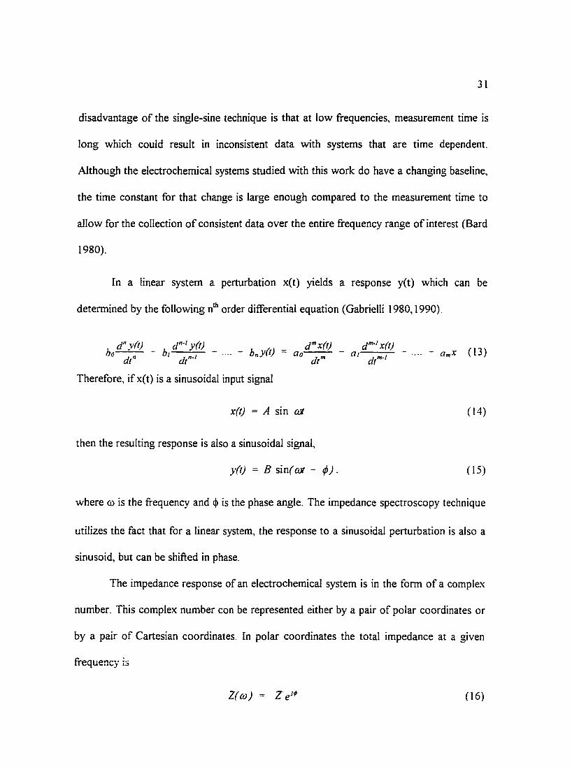
In a linear system a perturbation x(t) yields a response y(t) which can be
determined by the following nth order differential equation (Gabrielli 1980, 1990).
dn y{t) dn-l y{t) ho - b1 I - ···· - bn V(t)
~n ~~ •
dmx(t) ao m
dt
Therefore, ifx(t) is a sinusoidal input signal
x(t) = A sin ca ( 14)
then the resulting response is also a sinusoidal signal,
y(t) = B sin( rut - ¢). (15)
where ro is the frequency and $ is the phase angle. The impedance spectroscopy technique
utilizes the fact that for a linear system, the response to a sinusoidal perturbation is also a
sinusoid, but can be shifted in phase.
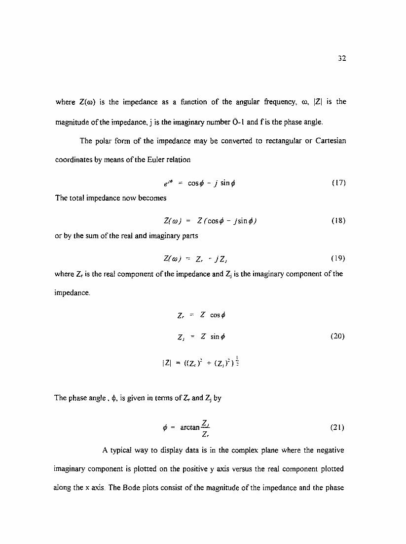
The impedance response of an electrochemical system is in the form of a complex
number. This complex number con be represented either by a pair of polar coordinates or
by a pair of Cartesian coordinates. In polar coordinates the total impedance at a given
frequency i::;
Z( w) (16)
..,? _,_
where Z( ro) is the impedance as a function of the angular frequency, ro, !ZI is the
magnitude of the impedance, j is the imaginary number 0-1 and fis the phase angle.
The polar form of the impedance may be converted to rectangular or Cartesian
coordinates by means of the Euler relation
e1; = cos¢ - j sin¢
The total impedance now becomes
Z( (1)) = Z (cos¢ - j sin¢)
or by the sum of the real and imaginary parts
Z( (1)) = Zr - } Z1
(17)
(18)
(19)
where Zr is the real component of the impedance and Zj is the imaginary component of the
impedance.
Zr Z cos¢
Z sin¢
The phase angle , ~, is given in terms of Zr and Zi by
¢ = arctan z 1
Zr
(20)
(21)
A typical way to display data is in the complex plane where the negative
imaginary component is plotted on the positive y axis versus the real component plotted
along the x axis. The Bode plots consist of the magnitude of the impedance and the phase

33
angle plotted against the log of frequency. The complex plane plot can be further dissected
into individual plots of real and imaginary components of impedance versus log of
frequency.
In order to model impedance spectra with a linear model, one must be careful to
use a small amplitude perturbation to ensure a linear response. Potential perturbation
dictates linearity in corrosion systems and typical values for potential amplitude fall
between 3.0 and 15.0 mV. The 'linear range' in which the amplitude must lie is determined
by the polarization point. The high limit of the linear range is the point where non linear
distortion begins and the low limit is determined by the signal to noise ratio. The maximum
permissible amplitude decreases with frequency, however, for convenience, a constant
perturbation amplitude is used for the entire frequency range for a given experiment. For
this reason, a thorough investigation of the low frequency response is needed in order to
properly set experimental parameters.
For this work numerical determination of linearity is conducted usmg a
measurement model approach developed by Agarwal et al.(1993b). This technique utilizes
a Voight equivalent circuit model which is consistent \vith the Kramers-Kronig relations to
determine whether complex quantities for a system satisfy the conditions of causality,
linearity and stability.
The basis for the typical EIS measurements is the application of either a potential
or current perturbation and the measurement of the resulting signal, current or potential
respectively. However, non-conventional techniques are being developed and are being
proven to be useful tools in the analysis of a vast variety of systems. In an electrochemical

34
cell the flow rate of electrolyte to the surface of the electrode can be perturbed
sinusoidally, and the resulting changes in current or potential measured. This is known as
electrohydrodynamic impedance spectroscopy. Work to develop particle characterization
techniques where electric fields are applied to a suspension of particles and the effective
transmittance of light through the suspension is measured as the resulting signal is
currently in progress. Modulation of the wavelength of light can also be used to perturb a
system, a good example being that of a semi-conducting material which responds to light
of different energies.
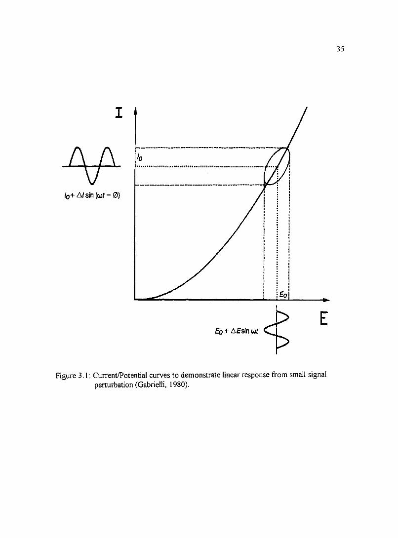
I
lo ·······························································
lo+ 6/ sin (wt- 0}
Eo
E Eo+~Esinwt
Figure 3. 1 : Current/Potential curves to demonstrate linear response from small signal perturbation (Gabrielli, 1980).
35

CHAPTER4 EXPERIMENTAL METHOD.
4.1 Impinging Jet System
The experimental design of this system was conceived in an effort to eliminate
problems with existing designs and incorporate new techniques. A submerged
axisymmetric impinging jet geometry was chosen for this study. The fluid mechanics
within the region of the electrode are well-defined and has been studied extensively
(Gilbert & LaQue 1954, Chin & Tsang 1978, Scholtz & Trass 1970a, 1970b ). This
geometry can be made to give uniform mass transfer rates across a disk electrode within
the stagnation region. The stagnation region is defined to be the region surrounding the
stagnation point in which the axial velocity is given by
(22)
and is independent of radial position, and the radial velocity is given by
d¢('7) v =ar--
r d'7 (23)
where a is the hydrodynamic constant which is a function only of geometry and fluid
velocity, r and z are the radial and axial positions, respectively, v is the kinematic
36

37
viscosity. and ¢ is the stream function which is given in terms of dimensionless axial
position '1 = z~ as (Chin & Tsang 1978)
Esteban et al. ( 1990) used ring electrodes to find that the stagnation region extends to a
radial distance roughly equal to the inside radius of the nozzle.
Within the stagnation region. the surface shear stress r~ is given by
I 3
rr= = -1312r(.upfa~ (25)
where Jl and p are the viscosity and density of the fluid, respectively. The hydrodynamic
constant can be determined experimentally using ring or disk electrodes at the mass
transfer limited condition. Shear stress on the electrode surface as a function of jet
velocity for the range of velocities used in this work is presented in Figure 4.1. A desired
value of shear can be reached at an exact radial position by adjusting the jet velocity. This
positioning of a specific shear stress is valuable when observing dramatic phenomena
which only occur above a specified shear. The shear stress values reported in Figure 4.l
can be compared to the critical shear stress values reported by Efird ( 1977) for copper
(9.6 N/m2) and 70/30 copper nickel (47.9 N/m2
).2
Mass transfer rate is uniform within the stagnation region; therefore, no
differential mass transfer cells can form near an electrode that lies entirely within the
stagnation region. The impinging jet system can therefore be used in the absence of
suspended particles to isolate the influence of the hydrodynamic shear stress. If the
removal of protective layers by hydrodynamic shear is the primary cause of erosion-

38
corrosion and the shear stress outside a certain critical radius is large enough to cause that
removal, then the metal outside the critical radius will corrode at a significantly higher
rate than the metal inside the critical radius. Since shear stress is a function of both radial
position and jet velocity, the critical radius corresponding to the critical shear stress
would be a function of jet velocity for fixed geometry.
-200
-180
-160 C\1
E-140 -. z --120 en en
~-100 -en ,_ ro -80 Q)
.r:. -60 en -40
-20
0 0 1 2 3 4 5 6 7
Jet Velocity, m/s
Figure 4.1: Shear stress as a function of jet velocity for the experimental work conducted here. The dimensionless quantity r/r0 represents the ratio of the radial position/electrode radius.

39
The ability to use optical techniques in situ with the impinging jet system allows
for the detection of radial variations on the electrode surface. In the current work,
impedance spectroscopy and computer-interfaced and enhanced optical microscopy are
used to provide information in-situ which can be coupled with potential measurements
and ex-situ analysis. Variable-amplitude galvanostatically modulated impedance
spectroscopy (Wojcik et al. 1996, 1997a,b,c) is an attractive technique because it can be
used in a non-invasive manner.
An electrically isolated, magnetic-drive centrifugal pump was utilized to produce
high flow rates without introduction of foreign species into solution. The impinging jet
cell was outfitted with two access ports, one at 45° and the other at 60° from vertical. The
primary objective of these ports was to allow in situ monitoring of the electrode surface
with a video microscope. The port not occupied by the video microscope was designed to
house probes to monitor cell conditions near the electrode surface. The electrochemical
impedance instrumentation consisted of a EG&G PAR 273 potentiostat and a Solartron
1260 Impedance/Gain-Phase Analyzer. The instrumentation was controlled by a PC using
Labview© and all interfacing code was written in-house.
A schematic of the experimental setup used in this work is shown in Figure 4.2.
The system consisted of the impinging jet electrochemical cell, main solution reservoir,
piping, pump, valves, connections, temperature controller and peripherals. The piping,
connections and reservoir were constructed of polypropylene. Cooling coils submerged in
the main reservoir to maintain the desired temperature were constructed of glass to obtain
better heat transfer than polypropylene and eliminate any sources of contamination,
40
present with more conductive metal materials. The coil temperatures were controlled by a
Fisher Scientific Isotemp Refrigerated Circulator model 910 and the pH of the solution
was measured and controlled in the main reservoir by means of a Cole-Parmer model
5652-10 pH!ORP controller. A saturated calomel reference electrode for the system was
also located in the main reservoir. The oxygen content of the solution was measured with
a Cole-Parmer oxygen meter model 5946-50 and the solution conductivity was measured
using a YSI Scientific model 35 conductance meter. The flow system pumped solution,
via a centrifugal pump powered by a VARIAC power supply, from the bottom of the
reservoir through a rotameter into the cell via the impinging jet and back to the main
reservoir. The jet velocity was adjustable from 1.0 m/s to 6. 75 m/s by modifying the
VARIAC output and/or the bypass line throttle valve position.
The experimental cell, displayed in Figure 4.3 consisted of a submerged,
axisymmetric impinging jet, a counter electrode, a working electrode with holder, an exit
port, and two windows for viewing the sample in-situ. Early experiments showed a need
for a large capacity cooling system ro combat the warming effect of viscous dissipation at
high velocities. To ensure accurate temperature control at the electrode surface, one of the
window ports was outfitted with a thermometer to monitor cell temperature for
comparison with reservoir temperature. The cell was constructed of acrylic sheet,
12.7mm thick and the base plate (bottom) of the cell was removable for access to the
interior of the cell. The counter electrode was located on the top of the cell, parallel to the
working electrode surface and was constructed of platinum foil of dimension 38.lmm x
50.8mm. The impinging jet was a 6.35mm I.D., 12.7mm 0.0. acrylic tube approximately
1.0 meter long that was adjustable laterally and vertically to ensure the jet was centered

41
over the sample (if desired) and to allow for different hiD ratios. The sample under study
was secured in the base plate of the cell by an adjustable sample holder which fixed the
sample flush with the bottom plate. Two observation ports, 19.0mm in diameter were
located in the two top-side plates of the cell. One of the observation ports was at a 45°
angle from the base plate and the other was at a 60° angle from the base plate. The 60°
angled port was retrofitted with the thermometer previously mentioned. These two angles
were determined in the design of the cell to be the optimum and most adaptable to
different electrode diameters respectively. The port windows were sapphire disks 4.5 mm
thick held in place with an aluminum retaining ring on the outside of the cell and sealed
on the interior with an o-ring. Chemical resistance to the synthetic sea water and optical
properties were key in selecting sapphire for the observation windows. Sapphire has the
optical property of high light transmission rates in the wavelengths of interest and scratch
resistance.
The experimental system was controlled and data was collected by a Gateway
2000 4DX2-66V personal computer. The software used to run the various experiments
was written in-house utilizing the graphical interfacing software Labview·. An EG&G
Princeton Applied Research (PAR) Model 273 potentiostatlgalvanostat and a
Schlumberger SI 1260 impedance/gain-phase analyzer were connected to the PC via a
GPIB connection. The PAR 273 controlled and measured the potential of the working
electrode and the SI 1260 superimposed a sinusoidal potential wave and calculated the
resulting impedance response.
42
The experimental cell was outfitted with a Hitachi color video camera model VK
C3 70 with a digital signal processor and a Navitar Zoom 6000 microscope lens system.
Digital images from the camera were captured by a Coreco Oculus-TCX True Color
Frame Grabber on the PC. These images were then viewed, processed, and stored. A
Dolan-Jenner high intensity illuminator series 180 equipped with fiber optic multi
directional wands was used to supply the necessary light to collect video images.
4.2 Sample and Solution Preparation
The working electrodes for this work were constructed of 6.35rnm diameter pure
copper and copper nickel alloy rods mounted with epoxy in a 41.3rnm diameter acrylic
sample holder referred to here as a puck. Before construction of the puck the copper was
annealed in a tube furnace at 750°C for 3.75 hours in an Argon atmosphere. A more
reliable annealing procedure was adopted during the course of this work. The new
technique involved annealing the rods in a vacuum furnace for 1 hour at 815°C. Initial
annealing procedures were subject to oxygen contamination. Discoloration in the surface
along the lines of flow of the argon gas were present after cooling of the sample. The new
technique did not cause non uniform discoloration of the surface after annealing.
After casting the electrodes in the puck using a two part epoxy purchased from
Buehler (part No. 20-8130-128, epoxide resin, No. 20-8132-032, epoxide hardener),
rough wet polishing was performed on the electrode starting with 180 grit paper and
working progrcssrvdy down to 600 grit paper. The final stages of polishing were
conducted using 1.0, 0.3, and 0.05 J.lm alumina powder, respectively, suspended on a
43
polishing cloth with de-ionized water. The sample was then cleaned with ethanol in an
ultrasonic bath for approximately 1 minute and inserted into the experimental cell. The
system was systematically flushed to remove any trapped air in the cell and tubing. The
electrolyte solution for the experiments was ASTM-D-1141 synthetic sea water which
was maintained at a pH between 8.05 and 8.3. To ensure constant light exposure to the
system, fluorescent lab lights were kept on and exterior light was eliminated for the
duration of each experiment. For capturing video images, additional lighting from an
external light source was temporarily employed.
The synthetic sea water solution was prepared with ASTM-D-1141 sea salts
which were combined with 2 M.Q deionized water. The solution was agitated and aerated
with C02 scrubbed air for no less than 2 days to allow the salt to dissolve completely and
to equilibrate the amount of dissolved 02. Early experiments were not aerated with a
pump, however, the large solution air interface in the reservoir and agitation from
solution circulation provided some aeration. The difference in solution 0 2 content
between the pump aerated and partially aerates solutions was 1.0ppm, 7 and 6 ppm
respectively. The solution was transferred to the experimental apparatus after the
preparation period and circulated, which quickly brought the electrolyte to the desired
temperature, 25°C.
4.3 Experimental Procedure
The series of experiments conducted for this work consisted of the monitoring of
open circuit potential over time, periodic impedance experiments, and periodic recording

44
of video images. Each of these procedures provides vital information in the analysis of
the corrosion mechanisms for the system.
The open circuit potential of the working electrode versus a saturated calomel
reference electrode was measured as a function of time by a PAR 273 potentiostat.
Periodically this measurement was suspended in order to conduct impedance experiments
and record video images of the surface, after which the open circuit potential was again
monitored. The open circuit potential value provides insight into the rate of corrosion and
the state of the system, and can be used to identify systems that are changing rapidly or
approaching a pseudo steady-state condition. All the electrodes tested for this work
changed rapidly at first and then reached a pseudo steady-state condition. Flow rates were
adjusted during the course of the experiments and the velocity effects on the impedance,
corrosion potential, and visual appearance of the electrode surface were investigated.
Impedance scans were performed in the variable-amplitude galvanostatically
modulated mode to prevent the introduction of a DC current driven by a shift in the
corrosion potential. Three or more impedance scans were generated at each point of
interest to verify reproducibility. For exploration of system with an unknown solution
resistance, an initial, limited potentiostatic scan was performed over a few points at high
frequency to determine the solution resistance, which was in turned supplied to the
galvanostatic program as the initial impedance guess.
Ambient lighting supplied by fluorescent lab lights proved to be insufficient to
illuminate the electrode to obtain a clear image capture. Therefore an external light source
was used to momentarily illuminate the electrode for the purpose of obtaining an image

45
grab. As predicted, this introduction of additional light caused slight disturbances to the
system due to the semi-conducting properties of the copper oxide films. Typically this
disturbance resulted in a slight reduction in the impedance. Through experimentally
monitoring the corrosion potential and impedance, it was determined that these minor
disturbances were reversible over a short period of time and had no effect on the long
term results.
Video images were utilized to learn about changes in the system over time, to
detect polishing flaws before an experiment, and to investigate a small area of the
electrode where an activity of interest may be taking place. Visual observation of the
images yielded information about how and if the surface was evolving as a function of
time. A key use of video images for this project was to determine if a radial dependence
of the reaction rate existed. This was accomplished by examining the images for rings or
halos which would suggest the presence of velocity-enhanced corrosion phenomena. The
video images captured for this work were acquired using the minimum magnification,
approximately 25X. The Hitachi camera and Navitar lens system used for this work both
have the ability to zoom in on the sample. Immediately after all air had been removed
from the system which took approximately three minutes, a video image was captured.
This image provided valuable information even before any electrochemical experiments
were conducted by exposing pre-existing flaws present on the surface of the electrode
which were not otherwise visible either without magnification or without submersion in
solution. Submersion made many flaws such as scratches more visible.
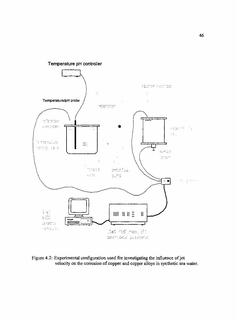
Temperature pH controller
Temperature/pH probe
··o:c:~:c·~r~·
•
Cf· ~: ~ ~·::: l c: . . :: . \ ~.
'. I ~\· D
, ·r•n ;.~ ; :,; ll
', ..... ," . · .. •,} . ...... \
Figure 4.2: Experimental configuration used for investigating the influence of jet velocity on the corrosion of copper and copper alloys in synthetic sea water.
46

. ~ ' . ' . \ '~ ~' .. ('
. ,j . ~- -·~ J\. ""' . '•' 1.,\ \:
: ~: :: 'J • : ; •
,,,..... . ,,,
( ~ i ' " ' ~ \1 ';
• ' ( ~ i ' • l ' ( ' ' l , ! • " ( : 1 • .. \.. - ... ' .....
-''' ·• '·'
Figure 4.3: Schematic illustration of the impinging jet cell and important cell components.
47
....:.··r··· . ..

CHAPTERS VARIABLE AMPLITUDE GALVANOSTATICALLY MODULATEDI~EDANCESPECTROSCOPY
The variable amplitude galvanostatically modulated impedance technique was
developed out of a necessity to conduct impedance scans on systems with changing
baselines. A good example of such a system is a corrosion system where the corrosion
potential is a function of time. Many factors can effect the characteristics of an
electrochemical system and some of these factors can cause rapid changes in the
corrosion potential. The potentiostatic as well as conventional galvanostatic methods of
conducting electrochemical impedance experiments both have inadequacies investigating
systems with a changing baseline.
Electrochemical impedance measurements are usually performed under
potentiostatic regulation. In these measurements the potential is a fixed value with a
superimposed (often sinusoidal) perturbation of fixed amplitude. This approach is
attractive because linearity in electrochemical systems is controlled by potential. For
example, a Taylor series expansion for current density at the open-circuit condition using
the Butler Volmer equation (Butler 1924)
(26)
yields
48
49
i = i {(a +a ) F'ls + (aa:!- ac 2) (F'ls )2 +(a/+ a/) (F'ls )3 + o('l "')} (27) o a c RT 2 RT 6 RT s
where aa and ac are the apparent transfer coefficients for the anodic and cathodic
reactions, respectively, lls is the surface overpotential, F is Faraday's constant, R is the
gas constant, and Tis absolute temperature. For typical parameter values for a symmetric
reaction (aa==ac=0.5) and for T=298 K, the second term is equal to zero, and the third
term is equal one percent of the first (linear) term for surface overpotentials of roughly
13.0 mV. Potential perturbations of 5 to 20 mV are often used. Potentiostatic regulation
is usually used even for measurement of the impedance at the corrosion potential, a
measurement which should, in principle, be conducted galvanostatically (with a time-
averaged current density set equal to zero). The potential is set to the value of the
corrosion potential at the beginning of the measurement and the potential is perturbed by
a value sufficiently small to ensure linearity (EG&G 1985, Schlumberger 1993).
The need for a small amplitude potential perturbation is even greater for typical
corrosion studies using impedance measurements conducted at the corrosion potential.
Close to the corrosion potential for steel, hydrogen evolution is unimportant, and the
oxidation of the metal can be assumed to be balanced by the mass transfer limited
reduction of oxygen. Thus, the total current density normal to the pipe surface is given by
(28)
where aFe is the apparent transfer coefficient for the oxidation of iron (or steel), io.Fe is the
exchange current density for the oxidation of iron, VFe is the equilibrium potential for the

50
oxidation of iron, V is the applied potential, and i0~ is the mass transfer limited current
density associated with reduction of oxygen. Note that a cathodic current is assumed to
be negative following the conventions used in electrochemical literature. At the corrosion
potential V= Vcorr, the net current in is equal to zero, and
(29)
An increase in the mass transfer limited current for oxygen reduction will shift the
corrosion potential to more positive values, and will, thereby, increase the rate of
corrosion. Equation (29) can be rewritten in terms of the corrosion potential as
(30)
At low current densities, linearization of the exponential term about the corrosion
potential yields
(31)
In contrast to the expansion for the Butler-Volmer reaction, the second term contributes
to the expansion and is equal to one percent of the first (linear) term for potentials as
small as 1.0 mV if aFc:=0.5.
Potentiostatic regulation is satisfactory for measurement of the impedance at the
corrosion potential if the corrosion potential does not change during the course of the
measurement. Under conditions where the corrosion potential is changing with time, the
potentiostatically-controlled impedance scan alters the behavior of the system under study
51
by forcing the potential to be constant during the period of the measurement. A
schematic representation of the influence of potentiostatically controlled impedance
spectroscopy on a system with a changing corrosion potential is given as Figure 5.1. The
potential decay represented in Figure 5.2 could be the result of growth of surface films
associated with corrosion products or calcareous deposits. The impedance measurement
in this case is invasive because the decay in potential is arrested during the measurement.
As illustrated in Figure 5.1, one consequence of the applying a fixed potential for a
system in which the corrosion potential would otherwise be changing is that the de
component of the current becomes non-zero. For corrosion measurements, the resulting
anodic or cathodic current can disrupt the growth of surface films and can lead to current
overloads.
Galvanostatic modulation of impedance experiments eliminates application of a
potential that is anodic or cathodic to the true open-circuit potential. Under galvanostatic
control, the desired zero-current baseline condition is maintained throughout the
impedance measurement, even when the corrosion potential drifts during the course of the
measurement of a impedance spectrum. The difficulty with galvanostatic measurements
with a fixed amplitude for the current perturbation is that such measurements can result in
severe swings in potential, especially at low frequencies where the impedance is large.
The amplitude of the potential variation Ll V associated with a perturbation amplitude of
current ill is given by

52
(32)
A current perturbation as small as 5 JlA can result in potential swings of 500 m V for
systems with a polarization resistance of 105 Ohms, a value typical of many membranes
and some slowly corroding systems, e.g., systems with well developed, dense films.
The potential swing associated with galvanostatically modulated impedance
measurements with a fixed perturbation amplitude can be significant even for systems
with a small polarization impedance. The potential perturbations resulting from three
fixed amplitude current perturbations on an RC circuit are shown in Figure 5.3. The
magnitude of the impedance for this system changed only one order of magnitude over
the entire frequency range. Yet, if a sufficiently large current amplitude is used to ensure
an acceptable signal-to-noise ratio at high frequency (e.g., 10 m V), the potential
perturbation at low frequency can be dangerously high and results here in a potential
swing of 100 mV (see triangles). For many systems a 100 mV perturbation is well above
the threshold defining linearity. Conversely, if care is taken to choose a current
perturbation which will ensure that the low frequency potential perturbation is within the
limits of linearity, the high frequency potential response can fall below the resolution
limits of the potentiostat.
An algorithm was developed in which galvanostatic regulation is conducted with
an amplitude of current perturbation that is adjusted at each frequency to yield a desired
variation in potential (Wojcik et al. 1996). This approach retains the advantage of

53
galvanostatic modulation that the experiment does not disturb the transients that would
otherwise exist in the system while ensuring the maximum signal-to-noise ratio for
perturbations that stay within the linear regime. The objective of this work is to present
recent improvements to the variable-amplitude galvanostatic modulation algorithm and to
demonstrate its utility for monitoring transient corrosion processes.
1.2
- 1 " >'
I 0
> --->8 0.8
::> -cu
-.:::;
a5 0.6 -0 a. UJ UJ ~ r::: 0.4 0 UJ r::: Q)
E a 0.2
0
-1
. . : Start Experiment
.. - ...... - ........ -- .t
' .. ..
I
: Start Potentiostatically : Controlled Impedance Scan I
. : ·._ .. I
·.
Finish Potentiostatically Controlled Impedance Scan
Perturbed Potential Decay
Unperturbed Potential Decay
0
'· : "• . '
1
. ·-
2
...
3
Dimensionless Time, th
..............
4 5
Figure 5.1: Schematic illustration of the influence of a potentiostatic impedance experiment on the corrosion potential of a system with a changing baseline.

~ rn c: (I)
Cl -c: (I) '-'-~ () rn
-0.1 rn (I)
c: 0 rn c: (I)
E Cl
Potentiostatic Control, V=O
Galvanostatic Control, 1=0
-0.05
10
5
-5
-10
Increasing Time
0.05
Surface Overpotential, V
0.1
Figure 5.2: Sequential current potential curves for a system with a transient corrosion potential.
54
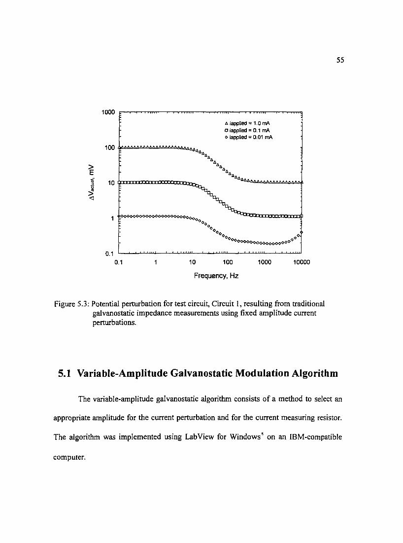
100
> E iij 10 "' ti
> <]
0.1 0.1 1 10
a iapplied = 1.0 mA a iapplied = 0.1 mA <> iapplied = 0.01 mA
100 1000
Frequency, Hz
10000
Figure 5.3: Potential perturbation for test circuit, Circuit 1, resulting from traditional galvanostatic impedance measurements using fixed amplitude current perturbations.
55
5.1 Variable-Amplitude Galvanostatic Modulation Algorithm
The variable-amplitude galvanostatic algorithm consists of a method to select an
appropriate amplitude for the current perturbation and for the current measuring resistor.
The algorithm was implemented using LabView for Windows~ on an IBM-compatible
computer.

56
5.2 Prediction of the Amplitude of the Current Perturbation
Measurements at previous frequencies are used to estimate the value of the
impedance at the target frequency. The current perturbation to be used is given by
- D.V ,6./ ( (j)) = target
jZ( (j) )jestimated (33)
where D.l ((j)) is the current perturbation at a given frequency, ~ ~arger is the desired
potential perturbation at the surface of the electrode, and !Z(ro)lestimated is the magnitude of
the impedance taken from the preceding measurement. In this approach, the magnitude of
the impedance at the frequency to be measured is predicted from values obtained at
previously measured frequencies. This prediction is therefore done without additional
probing of the system. A sequential collection of data in logarithmic increments of
decreasing frequency is assumed.
In early work (Wojcik et al. 1996), a one-point prediction algorithm was
employed which was defined by
Z(m,) = Z(m,_,) + o( lo{ :,•,)) (34)
where the impedance at frequency rok is assumed to be equal to the impedance at rok·l·
The error in equation (34) is of the order of the inverse number of points per decade. In
the present work (Wojcik & Orazem 1997a) equation (34) was replaced by
Z(m,) = 3Z(m,_,)- 3Z(m,_2 ) + Z(m,_3 ) + o(Iog( :,·,) r (35)
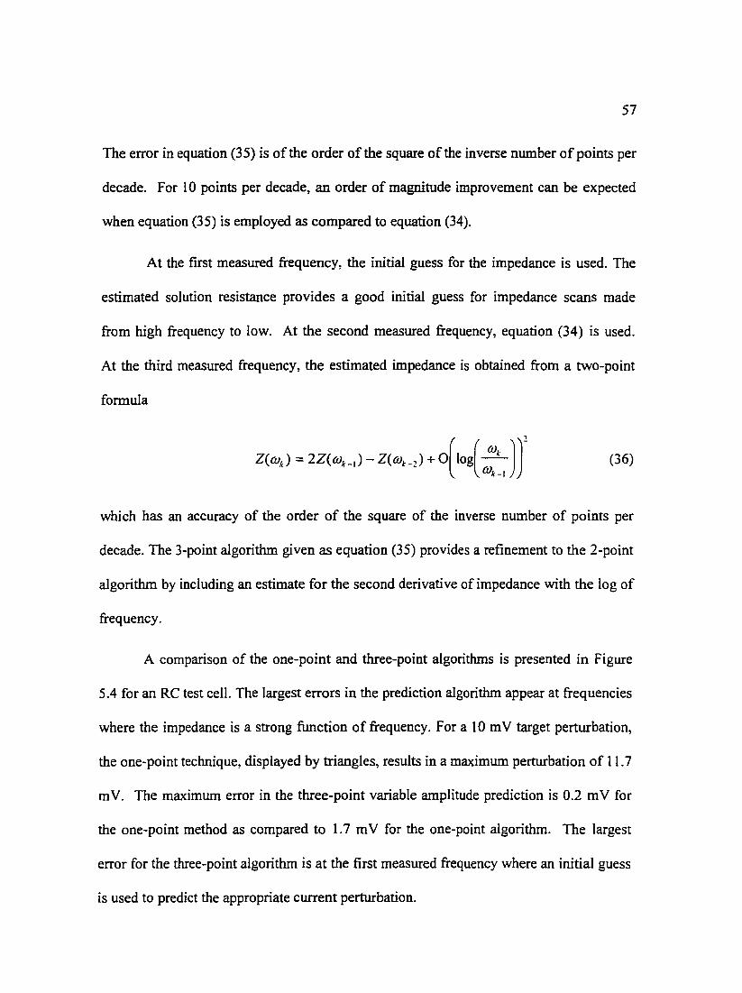
57
The error in equation (35) is of the order of the square of the inverse number of points per
decade. For 10 points per decade, an order of magnitude improvement can be expected
when equation (35) is employed as compared to equation (34).
At the first measured frequency, the initial guess for the impedance is used. The
estimated solution resistance provides a good initial guess for impedance scans made
from high frequency to low. At the second measured frequency, equation (34) is used.
At the third measured frequency, the estimated impedance is obtained from a two-point
formula
(36)
which has an accuracy of the order of the square of the inverse number of points per
decade. The 3-point algorithm given as equation (35) provides a refinement to the 2-point
algorithm by including an estimate for the second derivative of impedance with the log of
frequency.
A comparison of the one-point and three-point algorithms is presented in Figure
5.4 for an RC test cell. The largest errors in the prediction algorithm appear at frequencies
where the impedance is a strong function of frequency. For a lO mY target perturbation,
the one-point technique, displayed by triangles, results in a maximum perturbation of ll. 7
mY. The maximum error in the three-point variable amplitude prediction is 0.2 mY for
the one-point method as compared to l. 7 mY for the one-point algorithm. The largest
error for the three-point algorithm is at the first measured frequency where an initial guess
is used to predict the appropriate current perturbation.
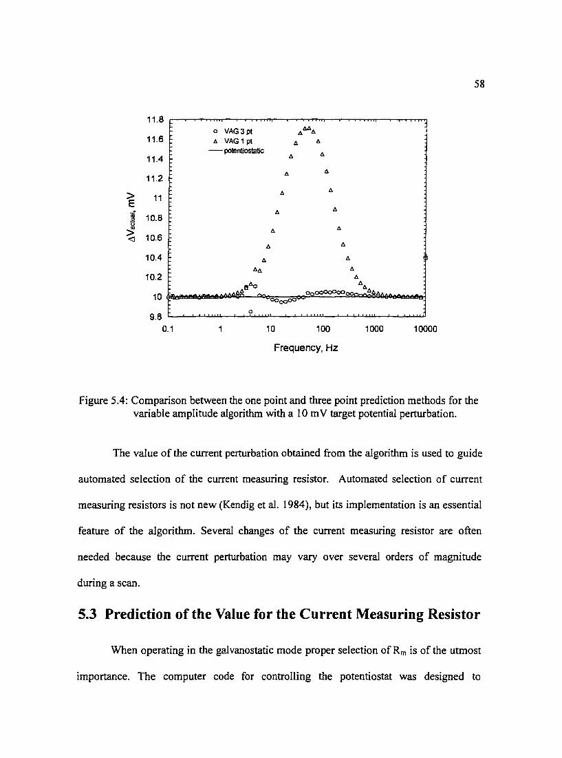
11.8
11.6
11.4
11.2
> 11 E iii 10.8 j
u "' > 10.6 <I
10.4
10.2
10
9.8 0.1
o VAG3pt t.. VAG 1 pt
- potentiostatic
0
1
58
10 100 1000 10000
Frequency, Hz
Figure 5.4: Comparison between the one point and three point prediction methods for the variable amplitude algorithm with a 1 0 m V target potential perturbation.
The value of the current perturbation obtained from the algorithm is used to guide
automated selection of the current measuring resistor. Automated selection of current
measuring resistors is not new (Kendig et al. 1984 ), but its implementation is an essential
feature of the algorithm. Several changes of the current measuring resistor are often
needed because the current perturbation may vary over several orders of magnitude
during a scan.
5.3 Prediction of the Value for the Current Measuring Resistor
When operating in the galvanostatic mode proper selection of Rm is of the utmost
importance. The computer code for controlling the potentiostat was designed to
59
automatically select the proper Rm for the current to be applied (refer to Table 5.1). To
compliment the algorithm used to predict the current perturbation at the next frequency,
an algorithm to determine the optimum current measuring resistor to be used was also
developed. The current measuring resistors available for the EG&G PAR
Potentiostat/Galvanostat Model 273 are presented in Table 5.1 along with the nominal
current ranges for each selection. Each of the current measuring resistors can measure
currents from 15 to 190% of the posted current magnitude with the exception of the lQ
resistor which can measure up to 200% of the posted current magnitude. Selection of the
proper current measuring resistor is crucial to ensure reliable data collection. Selection of
too large a current measuring resistor will result in a current overload in the potentiostat
while too small a current measuring resistor will introduce noise into the measurement
resulting in a poor signal to noise ratio.
One can observe from Table 5.1 that there is an overlap of adjacent resistor
values. As a rule of thumb, measurements that are conducted to the side of full range
measurements tend to be more sensitive than those taken at the lower limits of the
allowable range i.e. a current value of 17 rnA would be more accurately measured using
the 1 OOQ rather than the 1 OQ current measuring resistor. There are, however, situations
where the expected current from and electrochemical experiment is augmented by an
additional current present due to noise, external perturbation, or change in the system
under study. These unpredicted sources of current can cause difficulties if not handled
properly by the potentiostat. When the selection of the optimum current measuring
resistor is based solely on the perturbation being applied, the additional currents will in

60
many instances cause a current overload condition. With the new current measunng
resistor selection algorithm, a more conservative approach can be taken in situations
where overloads are common. The algorithm for selecting the proper current measuring
resistor was based on calculation of
frm:dt<"t log . = x.y
1mm
(37)
where x andy are the characteristic and mantissa of the logarithm, respectively, lpred1cr is
the predicted value for the current, and imin is the nominal minimum measurable current
for which the instrument, given in Table 5.1 to be 100 nA. A switch-over factor YcCan be
defined, which has a value between 1.5 and 1.9. If yS:yc, the current measuring resistor
index is obtained from kR = 7- x . lfy>yc, kR = 6- x . This algorithm has the feature
that it does not depend on past history, and increases or decreases in current measuring
resistor values are possible based on the predicted current value.
defined, which has a value between 1.5 and 1.9. If y5yc, the current measuring resistor
index is obtained from kR = 7- x . Ify>yc, kR = 6- x . This algorithm has the feature
that it does not depend on past history, and increases or decreases in current measuring
resistor values are possible based on the predicted current value.
Another important issue involving controlling current IS maintaining a zero
current condition before the initiation of an applied current. Instrumental limitations led
to control problems with this work before impedance scans were initiated. For example,
the PAR 273 potentiostat has a current measuring accuracy of 0.2% in the range I O!J.A to
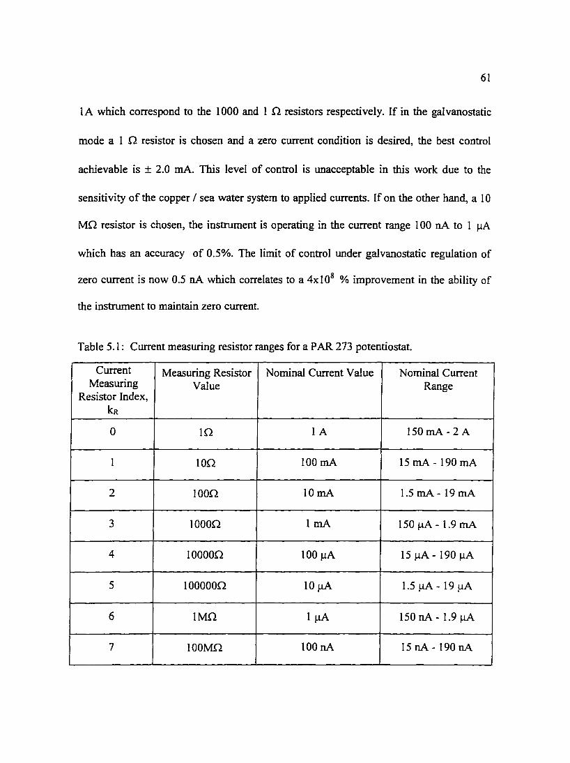
6I
IA which correspond to the I 000 and I .0. resistors respectively. If in the galvanostatic
mode a I 0 resistor is chosen and a zero current condition is desired, the best control
achievable is ± 2.0 rnA. This level of control is unacceptable in this work due to the
sensitivity of the copper I sea water system to applied currents. If on the other hand, a I 0
MO resistor is chosen, the instrument is operating in the current range I 00 nA to I J.lA
which has an accuracy of 0.5%. The limit of control under galvanostatic regulation of
zero current is now 0.5 nA which correlates to a 4x10⁸ % improvement in the ability of
the instrument to maintain zero current.
Table 5.1: Current measuring resistor ranges for a PAR 273 potentiostat.
Current Measuring Resistor Nominal Current Value Nominal Current Measuring Value Range
Resistor Index, kR
0 10 1A I 50 rnA- 2 A
1 IOO IOOmA I5 rnA - I 90 rnA
2 1000 IO rnA 1.5 rnA- 19 rnA
3 IOOOO I rnA I 50 !lA- 1.9 rnA
4 IOOOO.O. IOO J.lA I5 JlA- I90 J.lA
5 IOOOOOO IO J.lA 1.5 J.lA - I9 !lA
6 IMO IJ.!A I50 nA- I.9 J.lA
7 IOOMO IOO nA I5 nA- I90 nA
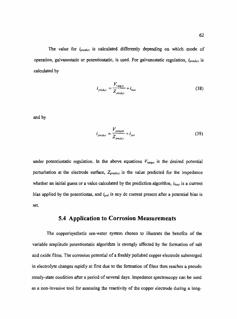
62
The value for ipredtcr is calculated differently depending on which mode of
operation, galvanostatic or potentiostatic, is used. For galvanostatic regulation, ipred1c1 is
calculated by
. V, arge1
l pn!dlcl = Z + i h10., rn:dlct
(38)
and by
(39)
under potentiostatic regulation. In the above equations V,arger is the desired potential
perturbation at the electrode surface, Zpredicr is the value predicted for the impedance
whether an initial guess or a value calculated by the prediction algorithm, hras is a current
bias applied by the potentiostat, and ipal is any de current present after a potential bias is
set.
5.4 Application to Corrosion Measurements
The copper/synthetic sea-water system chosen to illustrate the benefits of the
variable amplitude potentiostatic algorithm is strongly affected by the formation of salt
and oxide films. The corrosion potential of a freshly polished copper electrode submerged
in electrolyte changes rapidly at first due to the formation of films then reaches a pseudo
steady-state condition after a period of several days. Impedance spectroscopy can be used
as ~ non-invasive tool for assessing the reactivity of the copper electrode during a long-
63
term measurement of the corrosion potential if the amplitude of the perturbation is
sufficiently small and if the measurement does not perturb the baseline condition of the
electrode.
Potentiostatic experiments, due to their nature, do not maintain a zero current
condition throughout an experiment in which the corrosion.potential changes with time.
For a potentiostatic experiment, the corrosion potential is manually or automatically read
and a potential bias of that value is applied. The sinusoidal perturbation of an impedance
scan is then superimposed over this potential bias. If the open-circuit potential is stable,
the set bias will yield a zero or near zero current. If, however, the open-circuit potential
changes during the course of the experiment, in the latter stages of the measurement, the
bias potential will drive a anodic or cathodic current.
It is clear that potentiostatically regulated impedance measurements are invasive
for systems that have a changing corrosion or open-circuit potential. For such systems,
the zero-current condition can be assured only through use of galvanostatic control. For
conventional galvanic experiments, however, a fixed current amplitude is used which can
lead to poor signal-to-noise ratios, non-linearity, or both. Use of a single fixed value for
the current perturbation is inappropriate for the typical electrochemical systems
characterized by a magnitude of the impedance which varies over several orders of
magnitude with frequency. For the copper system used in this work the magnitude of the
impedance changed almost three orders of magnitude over the measured frequency range.
Data presented in Chapter 6 show a protective film on the surface of a copper
electrode disturbed by applied potentials as low as 50 mV. Higher impedance indicates a
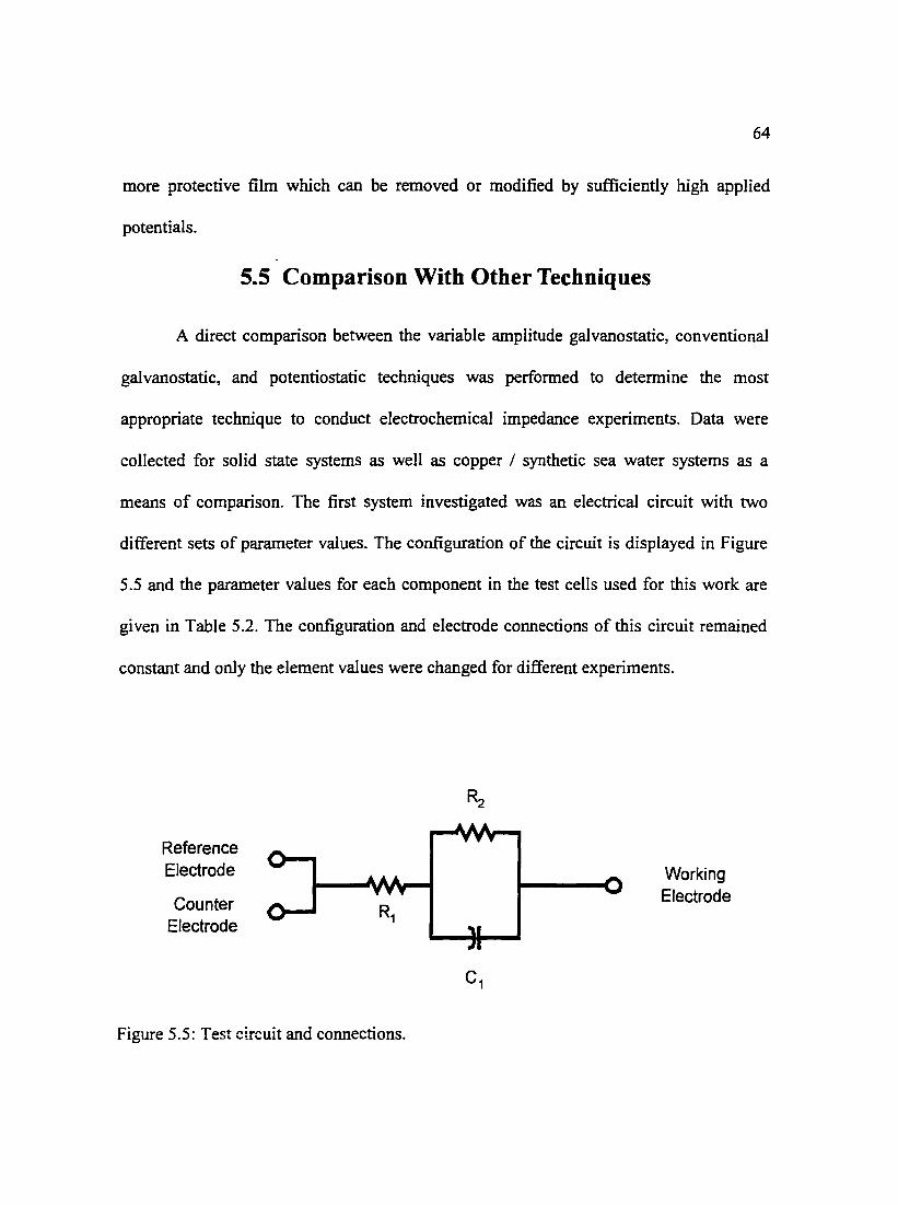
64
more protective film which can be removed or modified by sufficiently high applied
potentials.
5.5 Comparison With Other Techniques
A direct comparison between the variable amplitude galvanostatic, conventional
galvanostatic, and potentiostatic techniques was performed to determine the most
appropriate technique to conduct electrochemical impedance experiments. Data were
collected for solid state systems as well as copper I synthetic sea water systems as a
means of comparison. The first system investigated was an electrical circuit with two
different sets of parameter values. The configuration of the circuit is displayed in Figure
5.5 and the parameter values for each component in the test cells used for this work are
given in Table 5.2. The configuration and electrode connections of this circuit remained
constant and only the element values were changed for different experiments.
Reference Electrode
Counter Electrode
Figure 5.5: Test circuit and connections.
Working Electrode
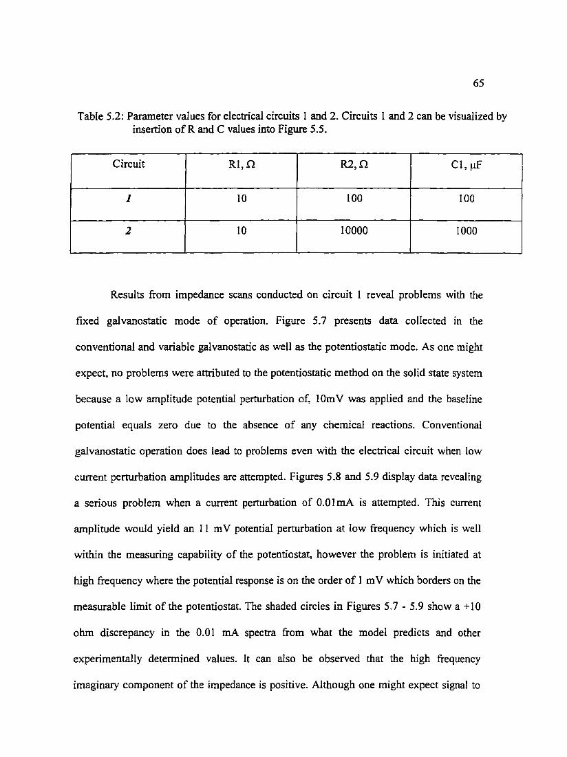
65
Table 5.2: Parameter values for electrical circuits I and 2. Circuits I and 2 can be visualized by insertion of Rand C values into Figure 5.5.
Circuit Rl,Q R2,n Cl, J..LF
1 10 100 100
2 10 10000 1000
Results from impedance scans conducted on circuit I reveal problems with the
fixed galvanostatic mode of operation. Figure 5.7 presents data collected in the
conventional and variable galvanostatic as well as the potentiostatic mode. As one might
expect, no problems were attributed to the potentiostatic method on the solid state system
because a low amplitude potential perturbation of, 1Om V was applied and the baseline
potential equals zero due to the absence of any chemical reactions. Conventional
galvanostatic operation does lead to problems even with the electrical circuit when low
current perturbation amplitudes are attempted. Figures 5.8 and 5.9 display data revealing
a serious problem when a current perturbation of 0.01mA is attempted. This current
amplitude would yield an 11 m V potential perturbation at low frequency which is well
within the measuring capability of the potentiostat, however the problem is initiated at
high frequency where the potential response is on the order of I mV which borders on the
measurable limit of the potentiostat. The shaded circles in Figures 5. 7 - 5. 9 show a + 10
ohm discrepancy in the 0.01 rnA spectra from what the model predicts and other
experimentally determined values. It can also be observed that the high frequency
imaginary component of the impedance is positive. Although one might expect signal to
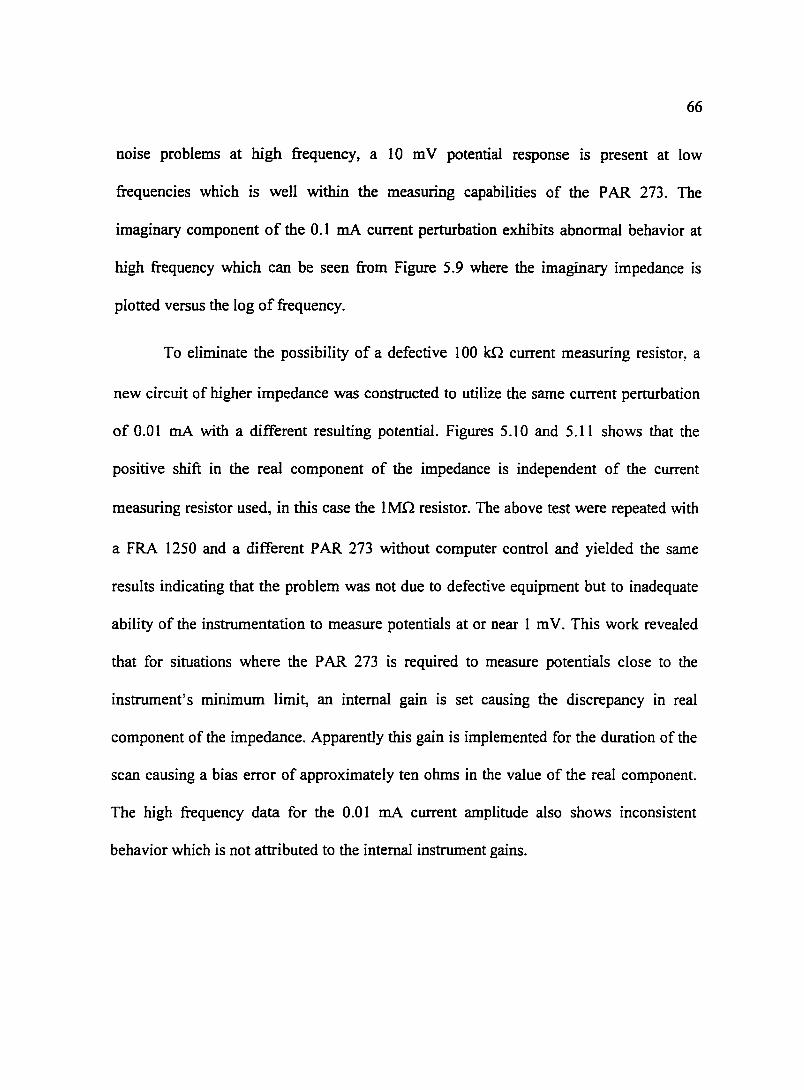
66
nmse problems at high frequency, a 10 m V potential response is present at low
frequencies which is well within the measuring capabilities of the PAR 273. The
imaginary component of the 0.1 mA current perturbation exhibits abnormal behavior at
high frequency which can be seen from Figure 5.9 where the imaginary impedance is
plotted versus the log of frequency.
To eliminate the possibility of a defective 100 kQ current measuring resistor, a
new circuit of higher impedance was constructed to utilize the same current perturbation
of 0.01 mA with a different resulting potential. Figures 5.10 and 5.11 shows that the
positive shift in the real component of the impedance is independent of the current
measuring resistor used, in this case the 1 MQ resistor. The above test were repeated with
a FRA 1250 and a different PAR 273 without computer control and yielded the same
results indicating that the problem was not due to defective equipment but to inadequate
ability of the instrumentation to measure potentials at or near 1 m V. This work revealed
that for situations where the PAR 273 is required to measure potentials close to the
instrument's minimum limit, an internal gain is set causing the discrepancy in real
component of the impedance. Apparently this gain is implemented for the duration of the
scan causing a bias error of approximately ten ohms in the value of the real component.
The high frequency data for the 0.01 mA current amplitude also shows inconsistent
behavior which is not attributed to the internal instrument gains.

-60
... • , • liD Jl) • liD • liD • liD • liD • liD • liD • liD • Jl:l •
-40
liD • Jl:l • r- liD • -20 Jl:l ; • 1 ; l
J 0
• • • • o iapplied = 1.0 mA
o iapplied = 0.1 mA
• • iapplied = 0.01 mA
40 r- cVAG 3 pt A Potentiostatic
r-
60 I
0 20 40 60 80 100
Figure 5.7: Impedance plane plot for test circuit Cell 1 comparing conventional galvanostatic, VAG, and potentiostatic techniques.
• , ~
67
l
120
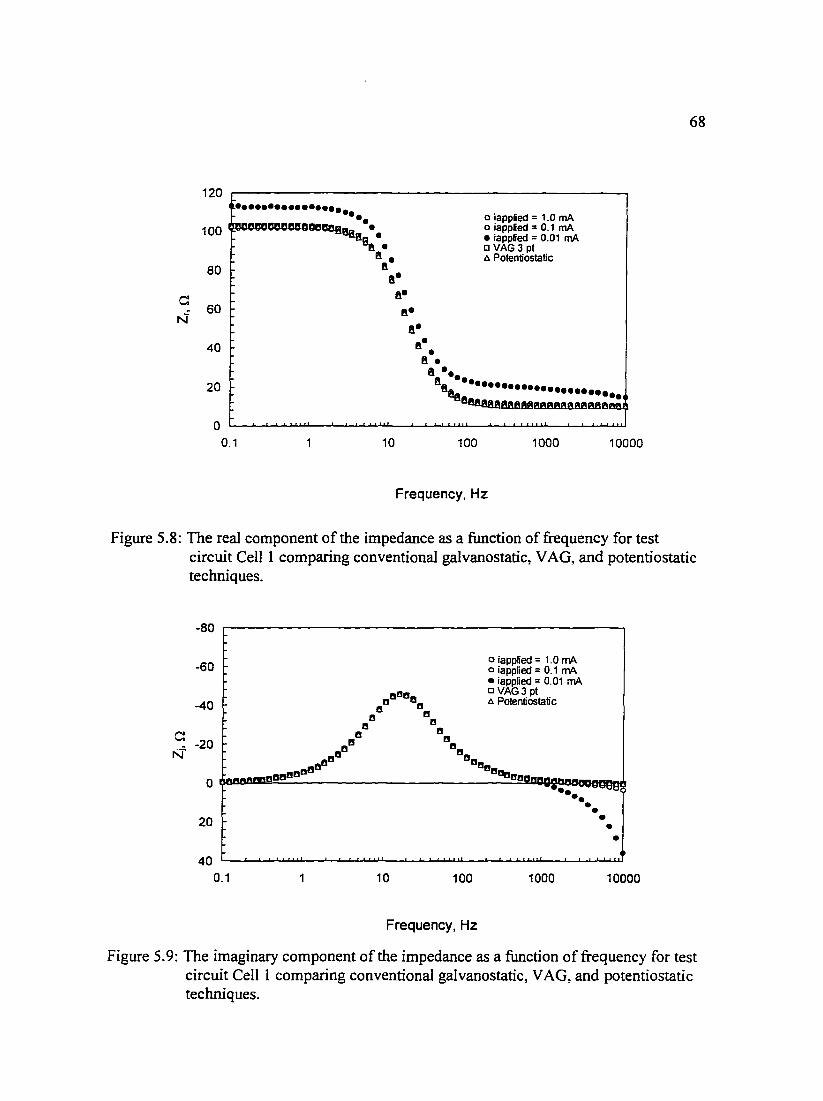
c: N
120 •••••••••••••••••
o iapplied = 1.0 rnA 100
•• ~DUOCOD~DOCt!Cam., • •
"DI!Be •• o iapplied = 0.1 rnA • iapplied = 0.01 rnA o VAG 3 pt
80
60
40
20
0 0.1
I! • I! ~t•
8..
!!!•
a• !.
t:J. Potentiostalic
• 8 • I! ••
I! •••••••• l!l!ft ••••••••••••••••• 8 1!l!MBMI!MIM!e!IM!e!IM!Me!l!!!!l
10 100 1000 10000
Frequency, Hz
68
Figure 5.8: The real component of the impedance as a function of frequency for test circuit Cell I comparing conventional galvanostatic, VAG, and potentiostatic techniques.
-80
-60
-40
c: -20
r't
0
20
40 0.1 10 100
Frequency, Hz
o iapp6ed = 1.0 rnA o iapp~ed = 0.1 mA • iapp~ed = 0.01 mA OVAG3pt t:J. Potentiostatic
•••• V<Jo
•• •• • • •
1000 10000
Figure 5.9: The imaginary component of the impedance as a function of frequency for test circuit Cell I comparing conventional galvanostatic, VAG, and potentiostatic techniques.

-800
-600 r-
4!IP • • • • • -400 a • • •
ell> • • •
-200 CD • c: B • ~ • "f
B • ~
f j i 0 I • • o 0.1 rnA, galvanostatic
• o 0.01mA, galvanostatic
200 • 0.001 rnA, galvanostatic 6. potentiostatic • oVAG
400 • 0 200 400 600 800 1000
Zr, Q
Figure 5.10: Impedance plane plot for test circuit Cell 2 comparing conventional galvanostatic, VAG, and potentiostatic techniques. Note the order of magnitude change in the impedance values compared to Cell 1.
• • '
69
1200
1200 1100
1000 900
800 700 600
c 500 .= 400
N 300 200 100
0 ..
-100 -200 -300
0.1
A AA
1
e•
•
• ... •
10
o 0.1mA, galvanostatic
a 0.01mA, galvanostatic
• 0.001mA, galvanostatic A 0.1 rnA, galvanostatic
A 0.01mA, galvanostatic
A 0.001mA, galvanostatic
100 1000 10000
Frequency, Hz
c N'
I
70
Figure 5.11: The real and imaginary components ofthe impedance as a function of frequency for test circuit Cell 2 comparing conventional galvanostatic, VAG, and potentiostatic techniques.

71
5.6 Experimental Studies
A comparison of techniques in Section 5.5 illustrated how the use of conventional
impedance techniques under given conditions can result in erroneous data. This is true
even for stable systems such as the electrical circuits used earlier to compare techniques.
The key strength to the VAG technique is, however, the ability to collect consistent data
even with difficult to measure systems such as those with transient baselines. The
copper/synthetic sea water system has the potential for a changing baseline or corrosion
potential with time, which can increase problems in the potentiostatic mode. Following
are several examples of data collected on a copper I synthetic sea water system using
potentiostatic, conventional galvanostatic, and VAG techniques. Impedance spectra
collected with the conventional potentiostatic and variable amplitude galvanostatic
modulation are presented in Figure 5.12. The three sequential variable amplitude
galvanostatic scans show good reproducibility. The subsequent three conventional
potentiostatic scans demonstrate significant differences, caused by imposition of an
anodic bias as the system changed with time. The conventional potentiostatic data can
be shown by the measurement model technique (Agarwal et al. 1992, Agarwal et al.
1993alb, Agarwal 1994, Agarwal et al. 1995alb) to be less consistent with the Kramers
Kronig relations than are the VAG data.
The large range of impedance values for this system makes it difficult if not
impossible to collect impedance data using the conventional galvanostatic techniques.
The problem is that, to retain an acceptable signal-to-noise ratio at high frequencies, the
perturbation must be sufficiently large as to cause a non-linear response at low
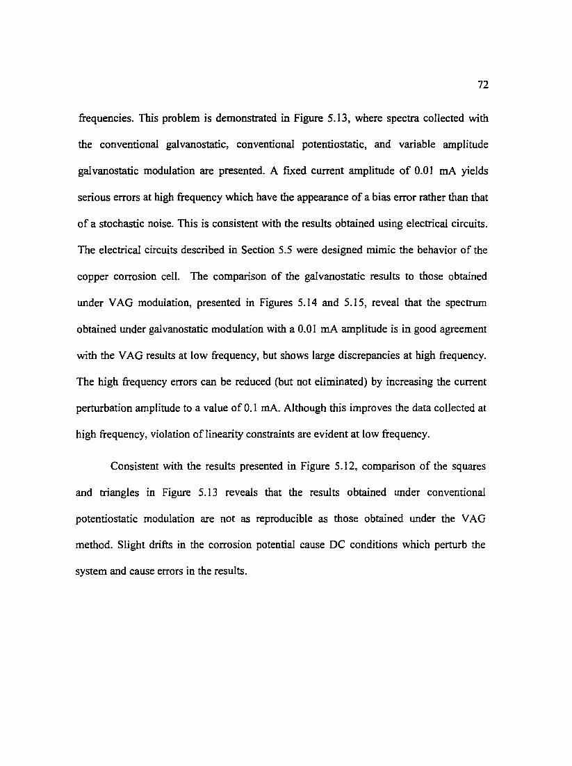
72
frequencies. This problem is demonstrated in Figure 5.13, where spectra collected with
the conventional galvanostatic, conventional potentiostatic, and variable amplitude
galvanostatic modulation are presented. A fixed current amplitude of 0.01 rnA yields
serious errors at high frequency which have the appearance of a bias error rather than that
of a stochastic noise. This is consistent with the results obtained using electrical circuits.
The electrical circuits described in Section 5.5 were designed mimic the behavior of the
copper corrosion cell. The comparison of the galvanostatic results to those obtained
under VAG modulation, presented in Figures 5.14 and 5.15, reveal that the spectrum
obtained under galvanostatic modulation with a 0.01 rnA amplitude is in good agreement
with the VAG results at low frequency, but shows large discrepancies at high frequency.
The high frequency errors can be reduced (but not eliminated) by increasing the current
perturbation amplitude to a value of 0.1 rnA. Although this improves the data collected at
high frequency, violation of linearity constraints are evident at low frequency.
Consistent with the results presented in Figure 5.12, comparison of the squares
and triangles in Figure 5.13 reveals that the results obtained under conventional
potentiostatic modulation are not as reproducible as those obtained under the VAG
method. Slight drifts in the corrosion potential cause DC conditions which perturb the
system and cause errors in the results.
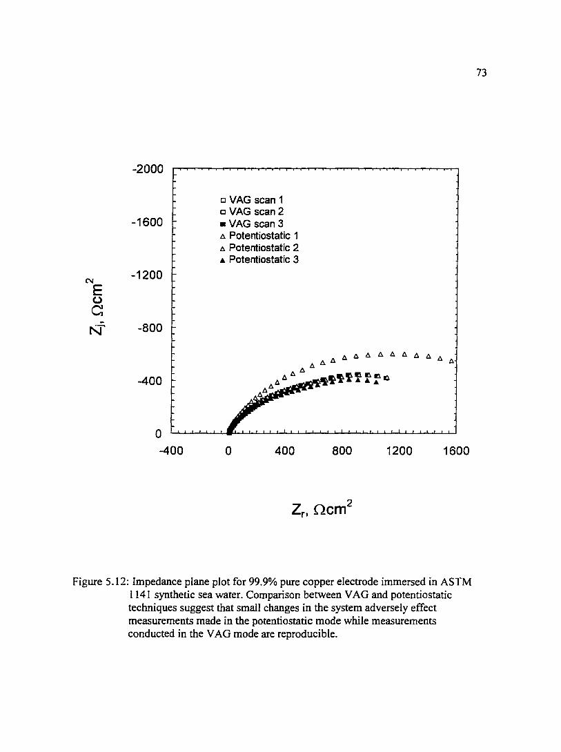
N
E (.)
c ~
-2000
-1600
-1200
-800
-400
0 -400
o VAG scan 1 o VAG scan 2 • VAG scan 3 ~ Potentiostatic 1 ~ Potentiostatic 2 • Potentiostatic 3
0 400 800 1200 1600
Figure 5.12: Impedance plane plot for 99.9% pure copper electrode immersed in ASTM 1141 synthetic sea water. Comparison between VAG and potentiostatic techniques suggest that small changes in the system adversely effect measurements made in the potentiostatic mode while measurements conducted in the VAG mode are reproducible.
73
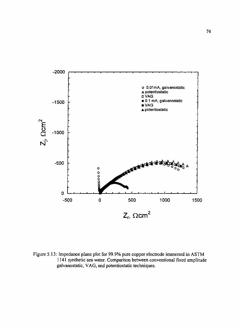
-2000
-1500
C\1
E (J c -1000
N-
-500
0
-500 0 500
o 0.01mA, galvanostatic A potentiostatic oVAG • 0.1 rnA, galvanostatic •VAG & potentiostatic
1000
74
1500
Figure 5.13: Impedance plane plot for 99.9% pure copper electrode immersed in ASTM 1141 synthetic sea water. Comparison between conventional fixed amplitude galvanostatic, VAG, and potentiostatic techniques.

N
E (.)
c: -= N
1500
1200
900
600
300
0
-300 0.1 1
o 0.01mA, galvanostatic cVAG •VAG • 0.1 mA, galvanostatic
10 100 1000 10000
Frequency, Hz
Figure 5.14: The real component of the impedance as a function of frequency for data presented in Figure 5.13. 99.9% copper immersed in synthetic sea water comparing conventional galvanostatic and VAG techniques.
-600
-500
-400 N
E u -300 c: r'j
-200
-100
0 0.1 1
o 0.01mA., galvanostatic o VAG •VAG • 0.1 mA. galvanostatic
0
0
0
10 100 1000 10000
Frequency, Hz
Figure 5.15: The imaginary component of the impedance as a function of frequency (see Figure 5.13) for 99.9% copper immersed in synthetic sea water comparing conventional galvanostatic and VAG techniques.
75
CHAPTER6 RESULTS AND DISCUSSION
Results for experiments conducted on copper and copper nickel alloy electrodes
are presented in this chapter. Electrochemical, X-ray photoelectron spectroscopy (XPS),
and digital image data were collected on the samples. Copper and copper alloys were
tested in a variety of environments, and the results were compared. Velocity, dissolved
02 content, and pH were among the experimental parameters adjusted and the response
to these changes is discussed in this section.
An important aspect of this work is the ability to predict the polarization
impedance of the system without a process model. With the use of the measurement
model, a value for the polarization impedance can be predicted. The measurement model
can be used to calculate the standard error of the prediction using a Monte Carlo
simulation. Section 6.1 of this chapter outlines the measurement model technique and
describes the utility of this method in analyzing impedance spectra in the absence of a
process model. The measurement model approach was applied to a variety of systems and
the results of the analysis are presented in Sections 6.3 through 6.6.
Electrochemical techniques used consisted of electrochemical impedance
spectroscopy, corrosion potential monitoring, and linear sweep voltammetry.
Electrochemical techniques provide insight into the state of the electrode surface and also
give information on the progress of film formation, modification, and/or removal.
Sections 6.3, 6.4, and 6.6 include results of 99.9% pure copper samples investigated in
76
77
aerated and partially-aerated solutions with dissolved 02 concentrations of 7.0 and 6.0
ppm, respectively. Aerated solutions were maintained by bubbling C02 scrubbed through
the solution with an electric pump. The partially aerated solutions were allowed an air
liquid interface where 0 2 and C02 could diffuse passively into solution. The response of
small changes to the pH (8.06 to 8.24) in the partially-aerated solutions had little effect
on the corrosion potential or the impedance response. Changes in the velocity, however,
had an observable effect on the corrosion potential and a large effect on the impedance.
In several experiments the impedance response was reduced by 50%. In well-aerated
solutions, velocity changes had little effect on the corrosion potential or the impedance
response. Results of experiments conducted on 70/30 copper/nickel alloys are presented
in Section 6.5.
The XPS technique was used to investigate species present on the surface of the
electrode after exposure to synthetic sea water, and digital imaging was used to maintain
a record of the condition of the surface throughout a run and to provide visual indications
of shear-induced corrosion.
All the electrochemical data collected during this work resulted from the
immersion of an electrode in ASTM 1141 synthetic sea water at 25° C. Potential
measurements were all conducted relative to a saturated calomel electrode (SCE). The jet
velocities investigated ranged from 0.0 to 6.2 mls at the jet nozzle. Aerated and partially
aerated solutions were examined and results of each were compared. The electrochemical
impedance spectroscopy technique used for this work was the VAG technique with a few
exceptions as noted. The copper-sea water system has the potential for a changing
baseline or corrosion potential which will accentuate problems in the potentiostatic mode.

78
6.1 The Measurement Model Approach
The differences in surface reactivity can be quantified, even in the absence of a
detailed mathematical model for the corrosion of copper, through use of the measurement
model approach. This quantification follows three steps:
I. Identification of the frequency-dependent error structure following the method
presented by Agarwal et al. (1992)
2. Identification of the portion of the spectrum that is consistent with the Kramers
Kronig relations following the method presented by Agarwal et al. (1993 a). High
frequency data were found to be corrupted by instrumental artifacts. The low
frequency data were typically found to be consistent with the Kramers-Kronig
relations except for data collected early in the experiment where the system was
changing rapidly.
3. Regression of the measurement model to the part of the spectrum found to be
consistent with the Kramers-Kronig relations using the error structure found in part I
above to weight the regression.
The regressed parameter values were used to extrapolate to the zero frequency limit, and
Monte Carlo simulations were performed using the standard deviations of the regressed
parameters to estimate the confidence interval for the extrapolation. The polarization
impedance was obtained by subtracting the regressed solution resistance from the
extrapolated zero-frequency value. The polarization impedance supplies a good
indication of how well a surface is protected, i.e. the corrosion resistance of the surface.
A knowledge of the predicted polarization impedance through the use of the
measurement model technique provides a powerful tool in materials selection for real-

79
world applications and can be equally beneficial in the field for determining in situ
materials performance.
6.2 Linear Sweep Voltammetry
Linear sweep voltammetry was used to investigate the formation of films on a
copper electrode under quiescent conditions. An aerated solution of synthetic sea water of
pH ~ 8.2 and 25°C was used as the electrolyte. Figure 6.1 .shows the current as a function
of potential, sweeping from a cathodic potential of -1.0 volts to the anodic potential of 1.0
volts. Figure 6.1 displays three linear sweeps of different rates ranging from 1.0 m VIs to
13.3 mV/s. The different sweep rates do not overlap indicating that the system was not at
an equilibrium state during the sweeps. This also suggests a mass transfer limited
condition because the currents were lower for the initial portion of the sweep. The
corrosion potential for a polished copper electrode in synthetic sea water is approximately
-300 mY versus SCE. The application ofthe initial cathodic potential shifted the potential
value corresponding to the zero current condition to lower values. This shift is more
significant at the faster sweep rate and at the slower rates, the zero current potential
approaches the equilibrium value. The anodic portion of the curve exhibits a higher
current for the 13.3 mV/s sweep which suggests that a thicker protective film had formed
during the 1.0 and 2.0 mV/s sweeps (Charriere 1997).
The four plateaus apparent in each of the sweeps presented in Figure 6.1 represent
regions where current was limited by mass transfer through surface films which increased
the impedance. The dotted line for the 1.0 mV/s has an inflection point where the current
drops at approximately -400 m V versus SCE. This suggests that a film formed protecting
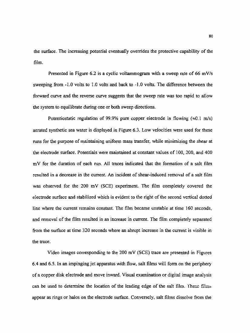
80
the surface. The increasing potential eventually overrides the protective capability of the
film.
Presented in Figure 6.2 is a cyclic voltammogram with a sweep rate of 66 mV/s
sweeping from -1.0 volts to 1.0 volts and back to -1.0 volts. The difference between the
forward curve and the reverse curve suggests that the sweep rate was too rapid to allow
the system to equilibrate during one or both sweep directions.
Potentiostatic regulation of 99.9% pure copper electrode in flowing (~0.1 m/s)
aerated synthetic sea water is displayed in Figure 6.3. Low velocities were used for these
runs for the purpose of maintaining uniform mass transfer, while minimizing the shear at
the electrode surface. Potentials were maintained at constant values of 1 00, 200, and 400
m V for the duration of each run. All traces indicated that the formation of a salt film
resulted in a decrease in the current. An incident of shear-induced removal of a salt film
was observed for the 200 m V (SCE) experiment. The film completely covered the
electrode surface and stabilized which is evident to the right of the second vertical dotted
line where the current remains constant. The film became unstable at time 160 seconds,
and removal of the film resulted in an increase in current. The film completely separated
from the surface at time 320 seconds where an abrupt increase in the current is visible in
the trace.
Video images corresponding to the 200 m V (SCE) trace are presented in Figures
6.4 and 6.5. In an impinging jet apparatus with flow, salt films will form on the periphery
of a copper disk electrode and move inward. Visual examination or digital image analysis
can be used to determine the location of the leading edge of the salt film. The::;e film~
appear as rings or halos on the electrode surface. Conversely, salt films dissolve from the

81
interior of the disk towards the outside. Figures 6.4 and 6.5 present images illustrating the
formation and dissolution of salt films on the surface of a copper electrode (order of
images is from left to right). The 200 mV (SCE) potential was applied and the
progression of the formation of the film can be observed in Figure 6.4. A plausible
explanation of the images in Figure 6.4 is that an anodic potential was applied resulting in
the formation of salt films. The first film, yellow in color can be seen in the first image of
Figure 6.4 and is pointed out by the arrow. The second film, which was more visible in
the second and third images with a darker, almost purple hue. This film gave way to a
third film, which can be seen near the periphery of the last image. Three possible
scenarios may have taken place. The first is that three different films formed and became
unstable and dissolved resulting in the formation of the other films. The second situation
involves three films forming at different times and being covered by the film which
formed next, and the third scenario is that one or more of the color changes is due to a
change in thickness of the film.
Removal of the salt film can be observed in Figure 6.5. The first image is of a
almost fully film-covered electrode, the film being yellowish orange in color. As time
passed the film lightened and began to break off in parts starting at the edge of the disk
due to a higher shear stress. The lightening of the film suggests a thinning effect,
however, the absence of the dark film suggests the presence of two different films. The
dark film was less stable than the orange-yellow film with a short residence time on the
disk at the given potential. A significant increase in the current (from 12 to 15 rnA) was
seen immediately following the loss of the large portion of film pointed out in the second
and third images by arrow (Charriere 1997). The salt films on the electrode surface were

82
not firmly adhered to the surface and were susceptible to shear stresses. The shear was
highest at the periphery of the disk resulting in the removal of the film on the outside of
the disk first. This work demonstrated the capability of the impinging jet video imaging
system to detect and monitor the radial dependence of film growth and dissolution, as
well as shear induced removal of films.
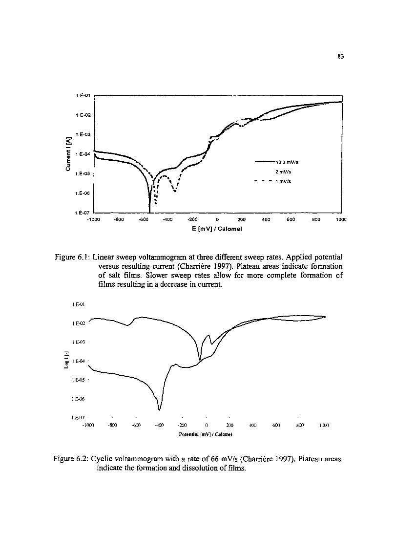
1.E-o1
1.E-02
1.E-03
~ ... c 1.E-o4 CD ... ... ::::l
(.) 1.E-OS
1.E-06
1.E-07 -1000 -800 -600
•• •• .. ..
-400 -200
,. .. .~
0 200
E [mV] I Calomel
---13.3 mVts
2 mV/s
- 1 mV/s
400 600
83
800 100C
Figure 6.1: Linear sweep voltammogram at three different sweep rates. Applied potential versus resulting current (Charriere 1997). Plateau areas indicate formation of salt films. Slower sweep rates allow for more complete formation of films resulting in a decrease in current.
I E-01
I E-02 ·
I E-03
~ I E-04 ·
I E-05 ·
IE-OS ·
I E-07
-loo:l -800 -600 -200 0 200 600 SOJ IOJO
Potential [mVI/ Calomel
Figure 6.2: Cyclic voltammogram with a rate of 66 mV/s (Charriere 1997). Plateau areas indicate the formation and dissolution of films.

84
0.04
0.03
+J c: ~ 0.02 s... :J (.)
0.01
0 0 200 400 600 800 1000
Time, s
Figure 6.3: Potential time traces for 99.9% pure copper in aerated synthetic sea water. Velocity C~ 0.1 m/s) maintained at low value primarily to ensure uniform mass transfer to the surface and removal of corrosion produces not tightly adhered to the surface.

85
Figure 6.4: Progression of a film growing during potentiostatic control at constant 200.0 m V. Images progress from left to right, total elapsed time = 1 000 seconds (Charriere 1997). Films originate at the periphery and grow towards the center of electrode.

\ -·.---: .::; ; ?·~-~_:.·~ - ..
·.-:: -- ·-·. :~-~- ~.:.::: .. :--~
_."-.·~-~-~--... ~--;.:"'--:··.:: .. . .. " ::.:·: ~"' . - .
~ •. ·..
.. -- ... \,· .. ··
86
Figure 6.5: Progression of a film removal from electrode surface during potentiostatic control at constant 200.0 m V. Images progress left to right, total elapsed time = I 000 seconds (Charriere 1997). Film became unstable and was removed by shear beginning at the outer edge because of a higher shear stress.
87
6.3 Copper in Partially-Aerated Electrolyte: Part 1
The time frame for the experiment presented here spans 33 days. The resulting
corrosion potential data, impedance data, and digital images, are identified by the time
from the start of the experiment. Changes in the jet velocity and adjustments in the pH
were conducted during the experiment, and the influence of these changes on the
corrosion potential, impedance, and surface appearance were investigated. A time line for
the experiment is presented in Table 6.1.
The working electrode was 99.9% pure copper immersed in synthetic sea water.
The corrosion potential is presented in Figure 6.6 as a function of time for the entire 33
day period. The initial corrosion potential behavior of all the copper and copper/nickel
alloys studied for this work was similar in the sense that the corrosion potential,
immediately after submersion, increased rapidly during the first few hours (Agarwal
1993a). For the freely corroding systems investigated in this work, the corrosion potential
became more positive from the initial measurement, and the rate of change slowed until a
constant value was reached. The difference between the initial value and the constant
value was as much as 70 mV.
The jet velocity for the first seven days was controlled at 1 m/s and the pH was
8.05. Corrosion potential data for the first seven days of the experiment are presented in
Figure 6.11. A pseudo-steady-state value of -283 m V for the corrosion potential was
reached after approximately 48 hours, and this value fluctuated by less than 2 m V over
the next five days. Impedance data collected over the first five hours of this run are
displayed in Figure 6.12. The common trend for the impedance collected over time was
88
that of an initial decrease in the impedance followed by an increase to a pseudo steady
state value. This steady-state value was typically achieved after several days. The
extrapolated values for the polarization impedance are presented in Figure 6.13 for scans
taken in the first 5 hours. The polarization impedance decreased with time in the initial
seven hours of an experiment. The extrapolated value for the polarization impedance was
used here to indicate the level to which the surface is protected.
The velocity was reduced to zero after seven days and was kept quiescent for 16
days. Flow was resumed at 1.0 mls and a series of impedance scans were conducted to
investigate changes in the electrode reactivity over the quiescent period. Figure 6.14
displays impedance scans taken before and after the 16 day quiescent period. Video
images of the copper surface revealed the presence of a thick film. Comparison of
impedance data sets at time= 158 and 551 hours revealed an increase in the impedance
over the period of time the solution was stagnant. Figures 6.7 and 6.8 show images of the
electrode before and directly after the quiescent period. One can observe a precipitate on
the electrode surface in Figure 6.8 which was providing additional protection of the
surface but was not strongly adhered. The blue green color suggests the presents of
cuprous chloride dihydrate (taken from Table 2.4). The first scan after the quiescent
period, presented in Figure 6.14 (shaded circles), was collected in the potentiostatic mode
to ensure potential perturbation of I 0 m V while all the other scans were collected in the
VAG mode. A slight discrepancy between potentiostatic and galvanostatic data is
attributed to the presence of a DC component generated by a difference in the applied
bias and the corrosion potential baseline, a necessary procedure in the potentiostatic
mode.
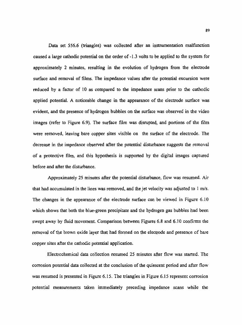
89
Data set 556.6 (triangles) was collected after an instrumentation malfunction
caused a large cathodic potential on the order of -1.3 volts to be applied to the system for
approximately 2 minutes, resulting in the evolution of hydrogen from the electrode
surface and removal of films. The impedance values after the potential excursion were
reduced by a factor of 1 0 as compared to the impedance scans prior to the cathodic
applied potential. A noticeable change in the appearance of the electrode surface was
evident, and the presence of hydrogen bubbles on the surface was observed in the video
images (refer to Figure 6.9). The surface film was disrupted, and portions of the film
were removed, leaving bare copper sites visible on the surface of the electrode. The
decrease in the impedance observed after the potential disturbance suggests the removal
of a protective film, and this hypothesis is supported by the digital images captured
before and after the disturbance.
Approximately 25 minutes after the potential disturbance, flow was resumed. Air
that had accumulated in the lines was removed, and the jet velocity was adjusted to 1 m/s.
The changes in the appearance of the electrode surface can be viewed in Figure 6.1 0
which shows that both the blue-green precipitate and the hydrogen gas bubbles had been
swept away by fluid movement. Comparison between Figures 6.8 and 6.10 confirms the
removal of the brown oxide layer that had formed on the electrode and presence of bare
copper sites after the cathodic potential application.
Electrochemical data collection resumed 25 minutes after flow was started. The
corrosion potential data collected at the conclusion of the quiescent period and after flow
was resumed is presented in Figure 6.15. The triangles in Figure 6.15 represent corrosion
potential measurements taken immediately preceding impedance scans while the

90
diamonds represent measurements taken immediately following these same scans. These
data were collected in the absence of flow. The pre-scan potential measurement are
reasonably constant at about -231mV, while the post-scan measurement showed more
variation due to the slight disturbances to the system caused by the measurement. After
potential disturbance and the flow was resumed the corrosion potential data are displayed
as circles in Figure 6.15. The outlying points around -340mV are attributed to the
application of the -1.3 volts previously discussed. As can be seen from the data, the
cathodic applied potential dramatically influenced the impedance response, corrosion
potential, and visual appearance of the electrode surface.
The corrosion potential returned to the value before the potential disturbance after
a period of 120 hours and remained constant for several days. A small adjustment of pH
by addition of NaOH had no discernible effect on the corrosion potential. The corrosion
potential changed abruptly, however, following an increase in jet velocities of 1.0 to 6. 75
m/s. The values for the shear stress corresponding to these velocities at a radial position
ofr/r0 = 0.8 are 14.5 and 195 N/m2, respectively.
Impedance data collected during this leg of the experiment are presented in Figure
6.16. It can be observed from Figure 6.16 that the impedance increased steadily after the
potential disturbance which corresponds to a decrease in reactivity as the protective films
reestablished. The value for the impedance was approaching a constant value after an
additional 150 hours. A pH modification from 8.05 to 8.24 had no discernible effect on
the impedance response when plotted in impedance plane format, however, the influence
of a change in jet velocity from 1.0 to 6. 75 mls on the impedance of the electrode is
easily seen in Figure 6.16.

91
The polarization impedances corresponding to impedance data displayed in
Figure 6.16 are shown in Figure 6.17 as a function of time. The general trend of the
impedance increasing over time can be observed. The sensitivity of the impedance
responses to changes in flow rate and pH can seen in Figure 6.16. The polarization
impedance and the associated confidence intervals given in Figure 6.17 were obtained by
the measurement model concept developed in this group as part of the infrastructure for
the erosion-corrosion experiments. The impedance response was found to be slightly
sensitive to the small adjustment of pH, and also shows a large increase in the reactivity
ofthe surface following the increase in jet velocity.
The video micrographs shown in Figures 6.18 through 6.21 give insight on the
evolution of the electrode surface. The polished copper electrode surface for the first
experiment discussed here is presented in Figure 6.18. This micrograph corresponds to a
time immediately after submersion in solution. Polishing marks not evident out of
solution by the naked eye can be observed in the micrograph. These polishing flaws were
left by the 0.05 micron alumina powder used in the final stage of wet polishing. An
evolution of the surface from the initial features can be seen in Figure 6.19 where a
uniform film was observable on the surface. After the system recovered from the
potential excursion, a similar uniform film was observed (Figure 6.21 ). The increase in
jet velocity resulted in a large reduction in the polarization impedance, however a
uniform film was still present on the electrode surface (Figure 6.21 ). The observable
increase in the sharpness of Figure 6.21 as compared to Figure 6.20 was attributed to
removal of a loosely adhered salt film. No ring-shaped features were evident in the

92
micrographs suggesting that the salt film was quickly removed when the velocity
changed and that the oxide layer below was still intact.
Table 6.1: Time line highlighting major events for the experiment presented in Figures 6.5 - 6.16.
Time, h Event
0 experiment start, u=1m/s, pH= 8.05, Figure 16a image captured
169 flow suspended, u=O mls, pH= 8.05, Figure 16b image captured
550-556 conduct impedance and corrosion potential measurements in quiescent
solution, pH = 8.13
556 applied potential of -1.3 volts,
557 flow initiated, u=1m/s, Figure 13 image captured
557 resumed standard collection of Ecorr and Z
671 Figure 16c image captured
718 pH change from 8.06 to 8.24
742 velocity change from 1 m/s to 6.8 m/s
814 Figure 17d image captured

-220
-240
-260 > E .= -280 .... 0 0 w
-300
-320
-340
U=1. m's
-,-. 0
Om's 1. m's 6.75 m's
0 96 192 288 384 480 576 672 768 864
Time, hours
93
Figure 6.6: Corrosion potential of 99.9% Cu measured as a function of time for a period of 33 days. Electrode remained in stagnant fluid from t= 190 to 550 hours. A cathodic potential was applied at t=556 hours and flow was resumed at t=557 hours.
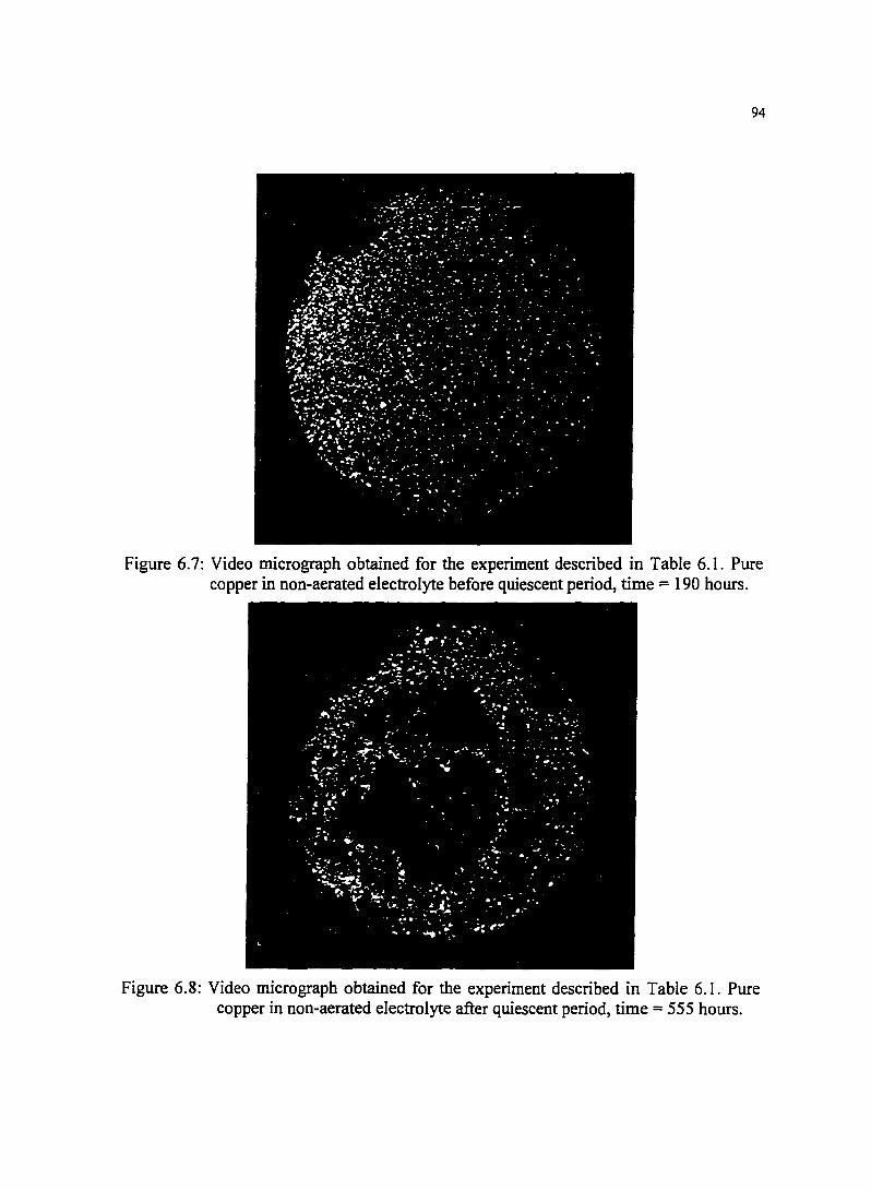
94
Figure 6.7: Video micrograph obtained for the experiment described in Table 6.1. Pure copper in non-aerated electrolyte before quiescent period, time = 190 hours.
Figure 6.8: Video micrograph obtained for the experiment described in Table 6.1. Pure copper in non-aerated electrolyte after quiescent period, time = 555 hours.
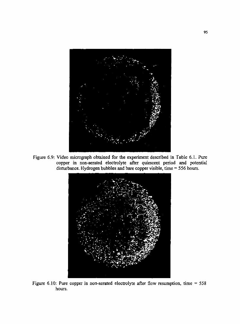
95
Figure 6.9: Video micrograph obtained for the experiment described in Table 6.1. Pure copper in non-aerated electrolyte after quiescent period and potential disturbance. Hydrogen bubbles and bare copper visible, time = 556 hours.
Figure 6.10: Pure copper in non-aerated electrolyte after flow resumption, time = 558 hours.

96
-250
-260
-270 1-
-280 r:- ------------------------------------ lin -------------------------
~
> -290
E -300 0 .... ....
0 0
w 8 -310 Q)
0
-320
~ -330
-340
-350
0 24 48 72 96 120 144 168
Time, hours
Figure 6.11 An expanded time scale for the Corrosion potential data presented in Figure 6.6. First seven days of immersion.
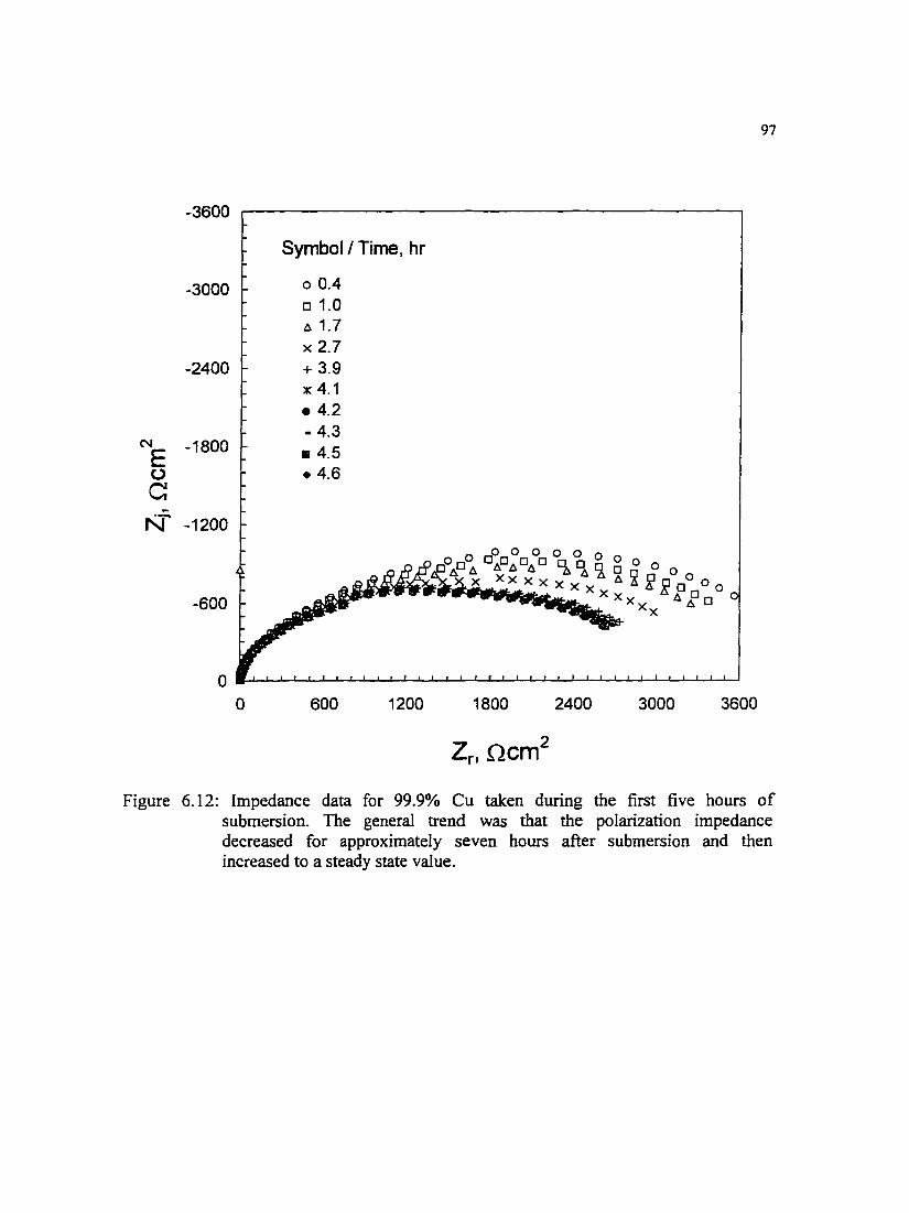
-3600
Symbol/ Time, hr
-3000 0 0.4 0 1.0 t:. 1.7 X 2.7
-2400 + 3.9
NE -1800
X 4.1 • 4.2 - 4.3 II 4.5
0 •4.6 c: N' -1200
0 600 1200
97
1800 2400 3000 3600
Figure 6.12: Impedance data for 99.9% Cu taken during the first five hours of submersion. The general trend was that the polarization impedance decreased for approximately seven hours after submersion and then increased to a steady state value.
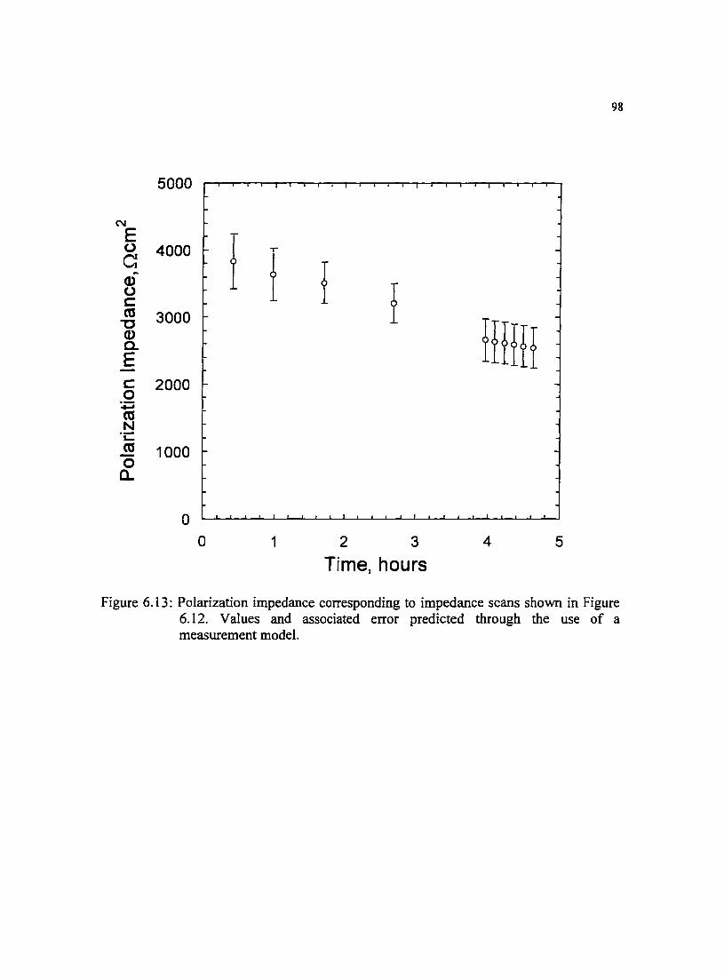
98
5000
C\1
E
f 0 4000 ~ I -c i I (J)
I 0 c: cu 3000 "'C
HHH (J) a. E c: 2000 0 ;; cu N
.i:: cu 1000 ~ --0 a..
0
0 1 2 3 4 5
Time, hours
Figure 6.13: Polarization impedance corresponding to impedance scans shown in Figure 6.12. Values and associated error predicted through the use of a measurement model.

-2500
-2000
-1500 C'll
E 0 • r'J -1000
-500
0 0
Symbol/ Time, hours
• 158.0 • 550.7 0 551.2 X 551.5 X 551.9 ~ 556.6
II II II II
-- --------
I
---
500 1000
• ,
--
1500
Zr, ncm2
99
' I II Ill • e C!J
0
2000 2500
Figure 6.14: Impedance scans for 99.9% Cu before and at the end of the 16 day quiescent period. Velocity for time=158 spectra was 1.0 rnls, all other scans the velocity was 0.0 mls
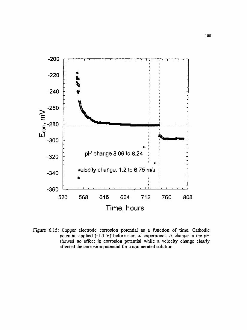
-200
-220
-240
-260 > E .:-280 .... -------------------~-----~----~---............. _....._.. __________________ -0 CJ w
-300
-320
-340
-360
520
-= pH change 8.06 to 8.24 ~
-= velocity change: 1.2 to 6. 75 m/s
•
568 616 664 712 760 808
Time, hours
100
Figure 6.15: Copper electrode corrosion potential as a function of time. Cathodic potential applied ( -1.3 V) before start of experiment. A change in the pH showed no effect in corrosion potential while a velocity change clearly affected the corrosion potential for a non-aerated solution.

N
E 0 c N"'
-1200
-1000
0 557.3 X 557.3 <> 588.4 l1 660.5
x 708.5 @ t=718: pH change 8.06 to 8.24 l1 732.5
-800 0 748.4 @ t=742: velocity change 1.0 to 6. 75 m/s
0 788.4
-600
-400
-200
0 0 200 400 800 1000
IOI
1200
Figure 6.16: Impedance data collected for 99.9% Cu over the course of the 231 hours corresponding to the corrosion potential data in Figure 6.15.
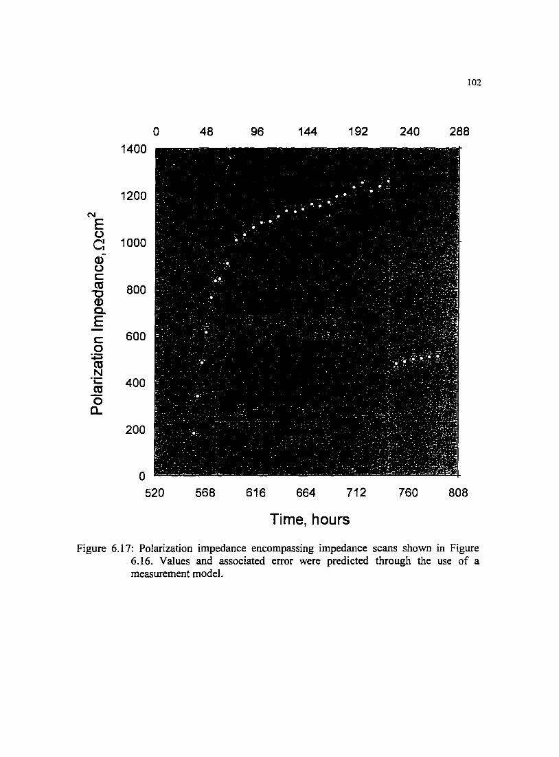
102
0 48 96 144 192 240 288 1400
1200 N
E (.)
c 1000 Q) (.) c: ca 800 "0 Q) a. E c: 600 0 ~ ca N
"i:: 400 ca 0 a..
200
0 520 568 616 664 712 760 808
Time, hours
Figure 6.17: Polarization impedance encompassing impedance scans shown in Figure 6.16. Values and associated error were predicted through the use of a measurement model.

103
Figure 6.18: Video micrograph obtained for the experiment described in Table 6.1. Pure copper in non-aerated electrolyte immediately after submersion, time = 0 hours. Polished state.
Figure 6.19: Video micrograph obtained for the experiment described in Table 6.1. Pure copper in non-aerated electrolyte at time = 169 hours.
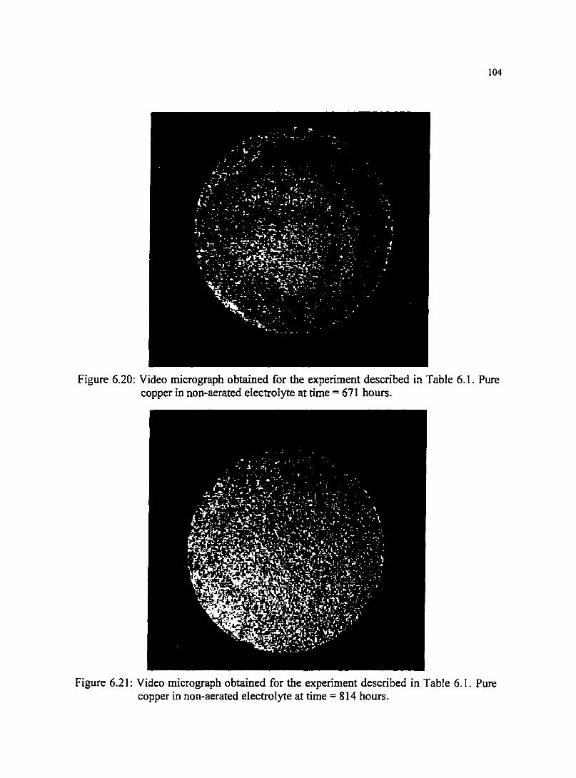
104
Figure 6.20: Video micrograph obtained for the experiment described in Table 6.1. Pure copper in non-aerated electrolyte at time= 671 hours.
Figure 6.21: Video micrograph obtained for the experiment described in Table 6.1. Pure copper in non-aerated electrolyte at time = 814 hours.
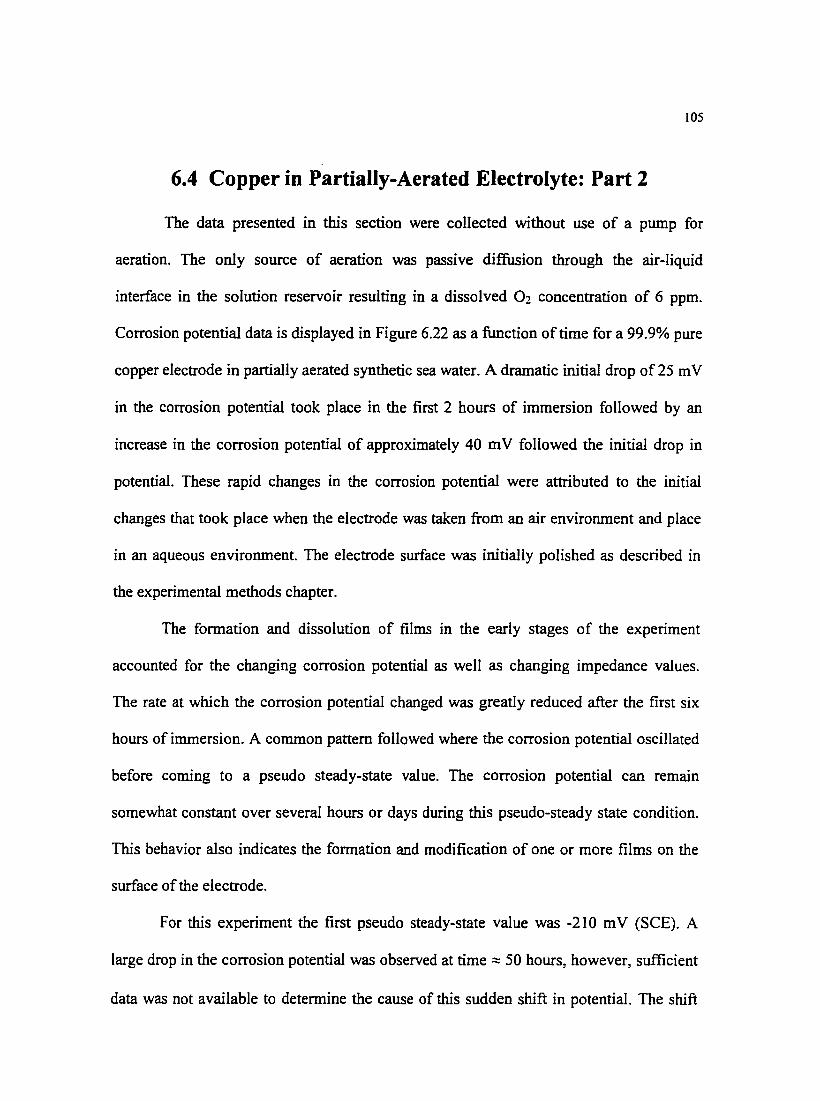
105
6.4 Copper in Partially-Aerated Electrolyte: Part 2
The data presented in this section were collected without use of a pump for
aeration. The only source of aeration was passive diffusion through the air-liquid
interface in the solution reservoir resulting in a dissolved 02 concentration of 6 ppm.
Corrosion potential data is displayed in Figure 6.22 as a function of time for a 99.9% pure
copper electrode in partially aerated synthetic sea water. A dramatic initial drop of 25 m V
in the corrosion potential took place in the first 2 hours of immersion followed by an
increase in the corrosion potential of approximately 40 m V followed the initial drop in
potential. These rapid changes in the corrosion potential were attributed to the initial
changes that took place when the electrode was taken from an air environment and place
in an aqueous environment. The electrode surface was initially polished as described in
the experimental methods chapter.
The formation and dissolution of films in the early stages of the experiment
accounted for the changing corrosion potential as well as changing impedance values.
The rate at which the corrosion potential changed was greatly reduced after the first six
hours of immersion. A common pattern followed where the corrosion potential oscillated
before coming to a pseudo steady-state value. The corrosion potential can remain
somewhat constant over several hours or days during this pseudo-steady state condition.
This behavior also indicates the formation and modification of one or more films on the
surface of the electrode.
For this experiment the first pseudo steady-state value was -210 mV (SCE). A
large drop in the corrosion potential was observed at time :::: 50 hours, however, sufficient
data was not available to determine the cause of this sudden shift in potential. The shift
106
could have resulted from an external perturbation in the form of pH and/or temperature
shift, or from a naturally oc~urring phenomenal within the system. After this disturbance
the system reac~ed a pseudo steady-state value of -223 mV (SCE) and remained at this
value,± lmV, until a modification in the flow rate was initiated.
Impedance spectra corresponding to the corrosion potential data in Figure 6.22 are
displayed in an impedance plane plot in Figure 6.23. One can observe a steady increase in
the impedance, as a function of time, until a constant value was reached, as indicated by
the shaded circles and stars in Figure 6.23. The corrosion potential was constant at -223
m V (SCE) and the impedance spectra were collected 18 hours apart with good
reproducibility. Experiments showed that even after the corrosion potential reached a
constant value the impedance of the system continued to increase until eventually
reaching a steady state condition. The impedance for this experiment reached and
maintained a constant value until the flow rate was adjusted from 2.0 to 6.2 m!s. The
increase in velocity resulted in an immediate decrease in the corrosion potential and
impedance. Both the impedance and the corrosion potential again stabilized after the
change in velocity, however, the values were different than the constant values before the
velocity. Two major phenomena contributed to the decrease in the impedance, the first
was an increase mass transfer of reacting species to the electrode surface. Also
contributing to the decrease in impedance was the dissolution of salt film on the surface
due to the velocity change. One can observe from Figure 6.23 that the impedance
increased slightly after the initial decrease caused by the velocity change. The impedance
eventually reached another pseudo steady-state condition. The higher flow prohibited the
modulus of the impedance from reaching the previously higher value.

107
Multiple impedance spectra were consecutively collected at the conclusion of this
experiment to investigate the effect of potential perturbation amplitudes on the surface ..
films. The velocity was maintained at 6.0 mls and the pH was 8.26. Several impedance
spectra were collected consecutively in the VAG mode and the perturbation amplitude
was incrementally increased with each scan. Periodically an impedance spectra was
collected with a low target amplitude, e.g. 5.0 to 15.0 mY, to ensure a linear response and
to determine whether previous the potential perturbation had disrupted or modified the
protective film on the surface of the electrode.
Perturbation potential as high as 40 m V had no lasting effect on the impedance of
the system, however, a perturbation potential of 50 m V dramatically effected the films
present on the electrode surface. One can observe from Figure 6.24 that the modulus of
the impedance irreversibly decreased by a factor of four due to the 50 m V potential
perturbation. This is an extremely important observation in that potentials on the order of
50 m V can be generated somewhat easily and could result in the disruption of a
protective film leading to premature failure of copper components in corrosion
environments. The films that were removed or modified would eventually grow back but
for the time frame of interest, this removal was irreversible.

108
-200 ,
-205
-210 0 _, CD ., 0
CD OC> .., 0 c)o..,_, 0 0 CXK) .., 0
-215 Oc:> 0 0 0
0 0 0 0 0
-220 0
> 0 0 00 C)
E C) ~ _, .v ., m 0 0 Cl[) :;:; -225 ClO r:::: 0 CD (1)0 ..0 Q)
0 -=> OC) -0 0 Q.
-230
-235 0
6.2 rnfs 2.0 mfs .... -240
....
-245
-250 0 20 40 60 80 100 120
Time, hr
Figure 6.22: Corrosion potential as a function of time for a 99.9% pure copper electrode in non-aerated ASTM 1141 electrolyte. Change in the corrosion potential due to velocity increase is evident.
140

-12000
-10000
-8000
N
E 0 -6000 c N~
-4000
-2000
0 0 2000
..elocity change 2.0 to 6.2 mls 95.75 hrs
eX e X f)
.x
4000 6000 8000
109
00.4 CJ 4.1 6 6.1 X 71.9 X76.5 • 94.9 - -99.5 & 121.4 • 144.0
e
e
0
10000 12000
Figure 6.23: Impedance collected on 99.9% copper over a period of 144 hours. The solution was not aerated and the effect of a velocity change from 2.0 to 6.2 rnls is observable.

110
-8000
1110 mV <> 15 mV t:.20mV
-6000 x25mV ·20mV o30mV +40mV osomv
N A 15mV E -4000 0 c N
~ O<f>+ ~+~~ + ~ -2000 a/4-,#4-
rJ> +>() ~
lifi!' t<o ~ <n-X+.
0 0 0
0
0 2000 4000 6000 8000
Figure 6.24: Nyquist plot for VAG experiments at different target amplitudes for 99.9% pure copper in non-aerated synthetic sea water. Effect of all amplitudes below 50.0 m V are reversible. An amplitude of 50.0m V dramatically and irreversibly changes the surface of the electrode.

Ill
6.5 70/30 Copper/Nickel Alloy in Aerated Electrolyte
The corrosion potential as a function of time for a 70/30 copper/nickel electrode
in synthetic sea water aerated with C02 scrubbed air is displayed in Figure 6.25. The
initial velocity was 2.0 m/s and the pH was 8.18. The initial drop and subsequent increase
in the corrosion potential was not as dramatic as seen with the 90/10 copper/nickel or the
pure copper. Similar to the other metals investigated, oscillations in the corrosion
potential were evident with the 70/30 alloy. The 70/30 copper/nickel alloy did not reach
a constant corrosion potential as quickly as did the copper, and, after eight days, the
corrosion potential was still increasing. This was an indication that the reactions at the
surface of the electrode was slower or thicker films were being formed. The copper
nickel alloy also displayed a higher sensitivity to impedance measurement. Disturbances
of up to 5 m V were seen after measurements. This disturbance to the system emanated
from a performance flaw in the potentiostat, where if the potentiostat is remotely
controlled, a mild potential was applied to the cell immediately after the remote cell on
command was initiated and .Le the first data point was collected. The higher
impedance values for this system lead to a greater potential disturbance for the same
current perturbation. The 70/30 alloy approached a pseudo steady-state potential of -200
m V (SCE) after an increase in velocity to 6.0 mls.
The impedance data corresponding to the corrosion potential plot in Figure 6.25
are presented in Figure 6.26. It is evident from the modulus of the impedance that the
70/30 alloy was more resistive to corrosion that was the pure copper. Impedance data
collected on the sample over a two week period tended to be less predictable than the
copper system. The modulus of the impedance increased and decreased in what seemed

112
to be a random manner throughout the entire experiment. A velocity change from 2.0 mls
to 6.0 mls resulted in a moderate change in both the corrosion potential and the
impedance values. Displayed in Figure 6.27 are data taken before and after the velocity
change. Multiple sets of three spectra were collected at each time indicated to ensure
reproducibility. The spectra collected I hour after the velocity change indicated a slight
decrease in the modulus.
Presented in Figure 6.28 is the polarization impedance of the 70/30 alloy. One
can observe how this value changed with time and also how the velocity change affected
the polarization impedance. The polarization resistance can assists scientist and engineer
assess the corrosion resistance of a material in the lab on in service in the field.
Comparison between the predicted values for polarization impedance of the 70/30
copper/nickel versus the pure copper indicates that the alloy would perform significantly
better (from a corrosion stand point, in sea water) than the pure copper.

-180
-185
-190
-195
> -200 E m
-205 +=0 c Q) -0 a. -210
-215
-220
-225
-230 0
<liD 0
CIID)()
«DCDDOO Oa::lOO 0
0 coo 0 ~ 000 0 00 0 0 0 0
-o oo• o ...... 00 <I»
...000000 CD ~-:> 0 00 •ooco o o o o o oo --ao CD :o 0 0 0 0.0 0 0 0 0 0 0 0 0 0 CJI) 0 0 :
0
0
00 00 <ID
OCD 00
00
0000000000 00 0 0 000000 0 0 0 0 00000 0 0 0 0
coo 0 moo 00 0 0
0 00 CD
G) 0 0
000
0
0
00
0
0
0
0 0 0
0 0
~locity change from 2 to 6 m's
48 96 144
Time, hours
192
0
240
0
113
288
Figure 6.25: Corrosion potential (SCE) data collected on 70/30 copper/nickel over a period of 288 hours. The solution was aerated with C02 scrubbed air and the effect of a velocity change from 2.0 to 6.0 m/s is observable.

114
-40000
Syrrbol/ Time, hrs
d 0.1 • 6.1 0
&17.2
-30000 X58.4 0
A64.4 %65.7 • 71.9
0 0
<> 96.1 0
N •124.0 0
E 0 X 0 -20000 -132.6
0 c d 182.3 0 0 X 0 196.1
0 X N 0 50.1 0 X d 0 xa d
0 xa 0 X
0 '!
d 0 - <>
-10000 GJ~-- <>.<>-:( '\:Xd- ~ - :( :(
~- - i.£e~ )!' r ••• ••••• • • A
A
0 ··~~~~~~~~--~~~~~~~~~--~~~~~
0 10000 20000 30000 40000
Figure 6.26: Impedance plane plot of several impedance spectra collected on a 70/30 copper/nickel alloy electrode with C02 scrubbed aeration over the course of 11 days. The susceptibility of the film to disturbance and measurement procedure is evident from the sporadic increase and decrease of the impedance values.
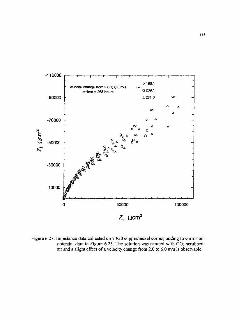
115
-110000
<> 196.1 velocity change from 2.0 to 6.0 I'TV's ..
at time = 268 hours 0 269.1
-90000 ~ 281.6 <0
<> ~ 00
~
-70000 <> ~
00 ~
N <> ~ 0
E m 10 ~
0 a -50000 r:?~
N
-30000
-10000
0 50000 100000
Figure 6.27: Impedance data collected on 70/30 copper/nickel corresponding to corrosion potential data in Figure 6.25. The solution was aerated with C02 scrubbed air and a slight effect of a velocity change from 2.0 to 6.0 mls is observable.

116
40000
35000 ~ N :
E 0 c: 30000
I 1 Q)
I f 0
f c:: 25000 as "0 Q) Q. :
E 20000 :
c:: i 0 +=- I
: as 15000 N ·c as 0 10000
CL
5000 velocity change from 2 to 6
rr/s -:
0 100 124 148 172 196 220 244 268 292
Time, hours
Figure 6.28: Polarization impedance predicted by the measurement model for 70/30 copper nickel alloy in synthetic sea water.
117
6.6 Copper in Aerated Electrolyte
The data presented in Figures 6.29 through 6.36 were collected on a copper
electrode in synthetic sea water aerated with C02 scrubbed air. The dissolved 0 2
concentration was 7.0 ppm and the pH was 8.2. The corrosion potential data for the
system is displayed in Figure 6.29. A cathodic potential of -414 mV was applied to the
electrode for 120 seconds after submersion and immediately prior to data collection to
remove oxide films which may have formed after electrode preparation. The initial decay
in the corrosion potential evident in each of the other experiments was not present in this
experiment due to the cathodic potential applied to the electrode. This potential removed
any oxide layer which formed after polishing and cleaning and during the time involved
in mounting the electrode in the cell base plate.
The initial velocity for this experiment was 1.0 rnls which was incrementally
increased over the 20 days of this experiment. The corrosion potential increased over the
first three days of immersion, as was characteristic of all other systems investigated in
this work. After reaching a maximum of -215 mV, the corrosion potential decreased at a
fairly constant rate until day ten. At this point the corrosion potential remained at -243,
±3 mV, until a velocity change was implemented 48 hours later. The velocity was
increased from 1.0 to 2.0 rnls resulting in a decrease of 2 m V in the baseline corrosion
potential. Figure 6.30 contains impedance data collected before and after the velocity
change. The constant value for the impedance displayed on the impedance plane plot of
Figure 6.30 indicates that a pseudo steady state condition had been reached before the
velocity change. The change in velocity had little effect on the magnitude of the
impedance which can be observed by the shaded diamonds and triangles in Figure 6.30

118
(taken immediately after and 26 hours after the velocity change). The slight decrease in
the magnitude of the impedance can be attributed to increased mass transfer of the
reactive species to the surface and not to removal of a film. Film removal is expected to
cause a dramatic reduction in the impedance.
The velocity was increased from 2.0 m/s to 4.0 m/s at time = 340 hours. This
increase in velocity had a minimal effect on both the corrosion potential and the
impedance response. Figure 6.29 displays a decrease of approximately 2.0 m V in the
corrosion potential. Impedance data collected before and after the velocity change are
presented in Figure 6.31. The system had again reached a pseudo steady state condition
before the velocity change which is apparent by the constant impedance values recorded
for greater than 24 hours preceding the velocity change. The increased mass transfer to
the surface had a slight effect in the impedance response which can be observed in Figure
6.3 I. A velocity change from 4.0 to 6.2 m/s yielded similar results. Figure 6.32 displays
impedance data before and after each velocity change and the overall difference in the
magnitude was small compared to what one would expect for velocity-enhanced
corrosion due to removal of an oxide film. Oxide films have a protective quality and
removal of these films would have resulted in a large reduction of the impedance. The
small changes in the corrosion potential and impedance response for each velocity change
in this case can be attributed to increased mass transfer to the surface and time dependent
characteristics of the system.
The polarization impedance of the copper electrode as a function of time for the
entire experiment is presented in Figure 6.33. The change in velocity had little effect on
the predicted polarization impedance, reaffirming the conclusion that shear removal of a

119
film was not present for this system even at the high shear rates present at velocities over
6.0 m!s.
The corrosion potential of the electrode for the first 24 hours of immersion is
presented in Figure 6.34. The effect of holding a cathodic potential on the electrode
before collecting data is evident. Figure 6.35 contains impedance data for the first 24
hours where the magnitude of the impedance decreases after immersion and reaches a
minimum around time = 8 hours. The decrease in the impedance may indicate a
roughening of the surface which is supported by video images. The magnitude of the
impedance increases after the minimum until a pseudo-steady-state condition is reached.
The corresponding polarization impedance predictions are displayed in Figure 6.36 where
an initial decrease in the polarization resistance is visible. This decrease is associated
with removal of native oxide layers that were not removed by the pre-polarization of the
electrode. The increase in the polarization impedance, after reaching a minimum,
indicated that the surface of the electrode was becoming increasingly resistant to
corrosion.
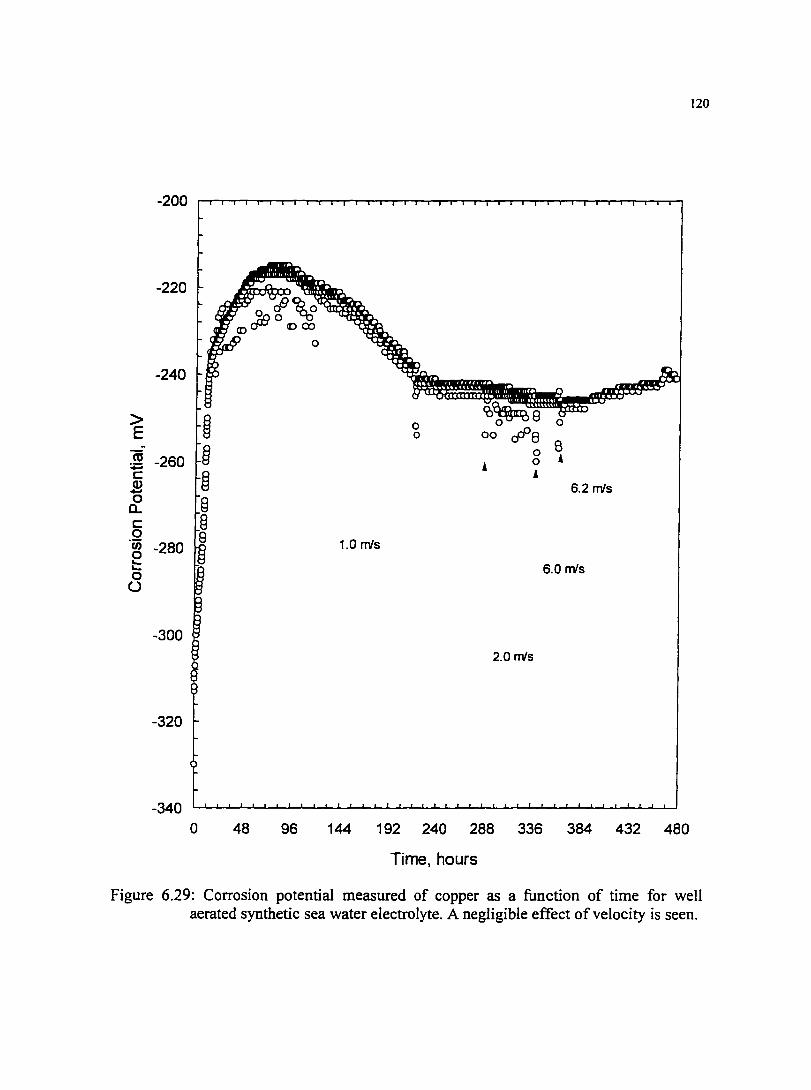
120
-200
-220
-240
> 0 E 0 00
m 0 8 -260 • 0 • +::: c: • Q) 6.2 mls -0 a.
c: 0 ·u; -280 1.0 mts 0 ....
6.0 mls .... 0 u
-300 2.0 mls
-320
-340 0 48 96 144 192 240 288 336 384 432 480
Time, hours
Figure 6.29: Corrosion potential measured of copper as a function of time for well aerated synthetic sea water electrolyte. A negligible effect of velocity is seen.
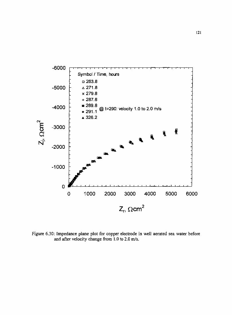
121
-6000 Symbol/ Time, hours
0 263.8
-5000 ~ 271.8 X 279.8 + 287.8
-4000 Ill 289.8 •
291_1
@ t=290: velocity 1.0 to 2.0 m/s
A 326.2 C'\1
E -3000 (J I c " ' ' r'J ' -2000 ' -----1000 --0
0 1000 2000 3000 4000 5000 6000
Figure 6.30: Impedance plane plot for copper electrode in well aerated sea water before and after velocity change from 1.0 to 2.0 mls.
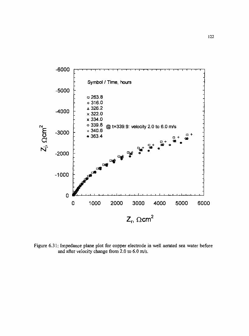
122
-6000
Symbol I Time, hours
-5000 0 263.8 0 316.0
-4000 ~ 326.2 X 322.0 :1: 334.0
N 0 339.8 @ t=339.9: velocity 2.0 to 6.0 m/s E -3000 + 340.6 0 • 363.4 o+
c 0 + ~ o+ Ill • O+ ~ e
rq 9.+ ot •
rvY • -2000 e
~D9 ~
-1000 ~ dl
0 0 1000 2000 3000 4000 5000 6000
Figure 6.3 I: Impedance plane plot for copper electrode in well aerated sea water before and after velocity change from 2.0 to 6.0 m!s.

-6000
-5000
-4000
C\1
E -3000 (.)
c ~
-2000
-1000
0
Symbol/ Time, hours
+ 239.8 o 263.8 @ t=290: velocity 1.0 to 2.0 m/s o 326.0 @ t=340: velocity 2.0 to 6.0 m/s ~ ~~~:j@ t=364: velocity 6.0 to 6.2 m/s X 476.3
5 t> 0~
'00 0 ~ "% ~
~ X
X X
+ 0 0
0 1 000 2000 3000 4000 5000 6000
Zr, ncm2
123
Figure 6.32: Impedance plane plot for copper electrode in well aerated sea water over the course of three velocity changes.

124
15000
@ t=290 h: velocity change from 1 m/s to 2 m/s
.: 12000
N
I I E
I If 0 c f I Q) I f: ! I 0
E f I c: 9000 m "'0 Q) 0..
I :
E c: :
: 0 6000 : +=i m N
f ·c m 0 :
0.. @ t=340 h: velocity change :
3000 : from 2.0 m/s to 4.0 m/s ... :
:
@ t=364 h: velocity change from 4.0 m/s to 6.2 m/s : ...
:
0 : :
0 96 192 288 384 480
Time, h
6.33: Predicted polarization impedance for aerated copper synthetic sea water system. Values and associated error predicted through the use of a measurement model. Error bars indicate the 95% confidence interval for each point predicted by a Monte Carlo simulation routine.

-200
-220
-240 ...
> E
E -26o Q) ..... 0
Q_
c ~ -280 0 ..... ..... 0 ()
-300
-320
-340
~
C)
0
125
0
•
4 8 12 16 20 24
Time, hours
Figure 6.34: Corrosion potential data for the first 24 hours for data presented in Figure 6.29.
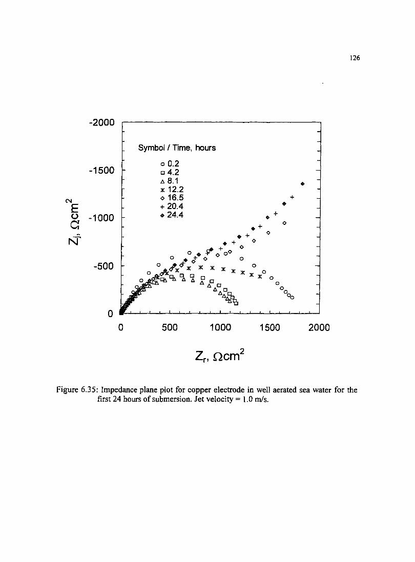
-2000
-1500
C\1
E (..)
c -1000
N"'
-500
0
0
Symbol/ Time, hours
0 0.2 D 4.2 A 8.1 X 12.2 0 16.5 + 20.4 • 24.4
500 1000
+ 0
1500
+ •
126
•
2000
Figure 6.35: Impedance plane plot for copper electrode in well aerated sea water for the first 24 hours of submersion. Jet velocity = 1.0 m/s.
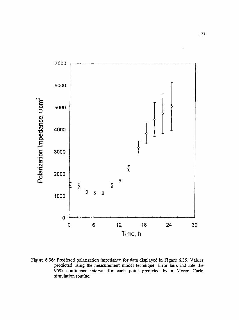
7000
6000
"' E c 5000
Q) (.) c: ~ 4000 Q) c.. E 5 3000
:.;::; rn N ·c rn 0 a.
2000
1000
0
127
2 Q Q
0 6 12 18 24 30
Time, h
Figure 6.36: Predicted polarization impedance for data displayed in Figure 6.35. Values predicted using the measurement model technique. Error bars indicate the 95% confidence interval for each point predicted by a Monte Carlo simulation routine.
128
6. 7 X-ray Photoelectron Spectroscopy Analysis
In order to investigate what species were present on the surface of a copper
electrode after submersion for a period of time, X-ray photoelectron spectroscopy was
employed. This analysis technique was implemented to obtain high resolution, high
magnification images of the electrode surface after exposure to sea water. XPS also
provided a semiquantitative tool for the comparison of element concentrations on the
surface of the electrode under different conditions. Concentrations differences related to
aeration technique are explored in this section.
X-ray photoelectron spectroscopy, or XPS, is a semiquantitative surface analysis
technique useful in investigating elements within the top ten atomic layers. XPS subjects
the sample of interest to a beam of X-rays causing emission of a photoelectron. The
photoelectrons are emitted from atoms near the surface and are detected by a
hemispherical analyzer located above the sample. The energy of the photoelectron is
equal to the difference in the X-ray energy, hu, and the electron's original binding energy,
Es.
E= hv-E8 -WF (40)
The work function, WF, of the specimen reduces the energy of the detected electron by a
small amount. The photoelectron energy is characteristic of the binding energy which
depends on the atom species and type of bonding. Therefore, the total number of
photoelectrons at a given energy reflects the concentration of a given species with a
particular type of bonding (MAl C).
129
XPS has applications ranging from investigating thin films and interfaces, to the
study of thermodynamically unstable species such as polymers, to identification of a
specimen's near surface composition. For this work XPS was utilized to determine
species present in the copper film and to compare results from films formed in partially
aerated solution and aerated solution. The data presented here is in the form of the x axis
representing the binding energy of the species and the y axis representing a normalized
energy, detected energy, or concentration of species with a given binding energy.
Characteristic photoelectron peaks for each element are plotted and the peak size reflects
the element concentration in a semiquantitative manner (MAIC).
Data presented in Figures 6.37 through 6.41 include XPS and scanning electron
microscope, SEM, data. The XPS data gave a semiquantitative analysis of what elements
were present at the surface and the concentration of these elements which in turn gives an
indication of what compounds were present. The corresponding SEM image in Figures
6.37,39-41 give a visual representation of the area that was analyzed by XPS. The
magnification of the SEM images ranged from 15X to 2000X.
Figures 6.3 7 and 6.3 8 contain data collected for a copper electrode previously
exposed in partially aerated sea water. The dissolved 0 2 content was 6.0 ppm. Solutions
that are not vigorously aerated with C02 scrubbed air will absorb C02 from the
atmosphere and this dissolved C02 will react with species in solution to form complexes
and acids, shifting the pH to a more acidic value. C02 production, consumption and
dissolution into solution plays a strong role in the regulation of pH in natural waters
(Stumm 1981 ). A slight decrease in the pH (pH=8.17) of the solution for this experiment

130
was seen due to C02 absorption. The number of species present at the surface are
considerably less than with aerated solutions.
Figures 6.39 through 6.41 display XPS data and SEM micrograghs a copper
electrode previously exposed in aerated sea water. Each data set was obtained at different
magnification or location on the electrode surface. The pH for this experiment, which
used the same solution as for the partially aerated case, was approximately 8.27. The
increase in the pH can be attributed solely to the removal of dissolved C02• A slight
increase in the bulk pH can cause enough of a change in the local pH to support a variety
of film which were not stable in less alkaline environments. Elements including
aluminum, magnesium, potasium, calcium, and iron are all distinguishable on the XPS
traces when an aerated solution was the electrolye These species complex to make salt,
oxide, or other films which are stable in more alkaline environments. One can observe
from Figures 6.40 and 6.41 a reduction in the copper species at the surface which was
attributed to the selective reaction with the other species and the covering of the surface
with films not containing copper. A more significant amount of copper is observable
Figure 6.39 because the area analyzed is large and portions of the electrode are not
covered by copper deficient films.
The XPS data supports the conclusion that the absorption rate of C02 was higher
with the passive aeration than with the forced aeration. The higher concentration of
dissolved C02 resulted in a slight decrease in the bulk pH which shifted the equilibrium
of the system to allow films of different composition to form on the surface and be stable.
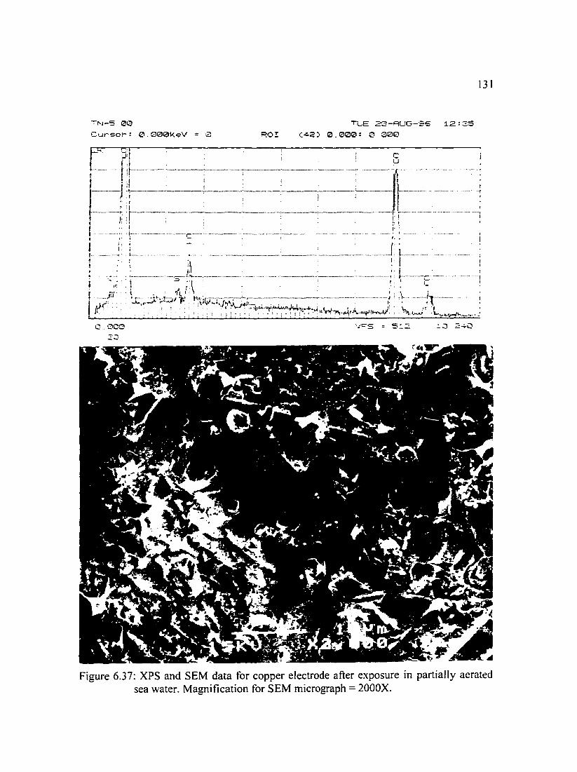
131
TI'J-5 0G
Cursor: 0.000KeV = 2 RO! TLE ?3-AUG-96 12:35
C42) 0.000: 0 G00
~ r• -~~ r i! . 0
........ ··t
I ······· .,
I : ~-- ······-····r-···-··- ·······--······· .. ········· ··- ·········'···-·· -· .... . .. ······ .. .... r· ; .... . ............. . . ' - . ,_ . I
I r ; . . , I·· I L.... .. ·····---.------------ ··-----···-··-··· ·-·-·············-·· ·······-· ......... .J. l .. . ; I I
.......... ------------· __________ lL ______________________ . _____ ..... ______ ------------------------·------· ... :: t--------------~--------· ... , I ·~I;. I .=> • ~ I. ; j~ I
I ?'" . \c~""''"'/~. h~:';/~c,·~=:;:;-:~?~~~.~~:=:~~.j • . ~,_:;ir~_ .... O.GCCl
Figure 6.37: XPS and SEM data for copper electrode after exposure in partially aerated sea water. Magnification for SEM micrograph= 2000X.

TN-5 121121 Cursor: 0.12100KeV = 121 ROI
TUE 2121-AUG-96 12:35 (42) 0.12100: 0.0121121
~ ' t u
--~-----~
: ::.
:._!_ . .__ __ i -, .::,i_:
= i r ,:----:-----I-----~------~-
~-----~; ,,___ r ---~ ---r---r-___ ;_l._· i_l._: ----r--E--·i--1 ___ : : ~ : : : : I
------t--· --, n----~--~-~ =c=i~
0.000
30
VFS = 512
; :
6"1-----------y-; ;
10 240
Figure 6.38: XPS data for copper electrode after exposure in partially aerated sea \Vater. Analysis for entire electrode surface.
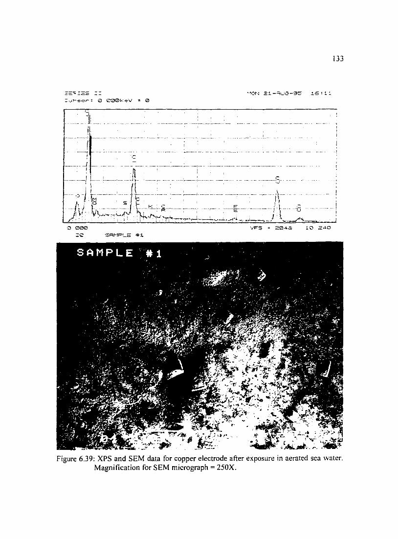
I '11- ....... . ll .
·····-· -·-···-----1
----------·· i '
····-· ...•.. ... ( !
VFS = 204..:;
1.,., .J.J
. !
Figure 6.39: XPS and SEM data for copper electrode after exposure in aerated sea water. Magnification for SEM micrograph= 250X.

134
·~EPIES ::::
:= -~~sc-: 0 •3001< ~·.1 0
Figure 6.40: XPS and SEM data for copper electrode after exposure in aerated sea water. Magnification for SEM micrograph = 250X.

....... ~--------- ······-·· ~----· ----:··········
:::l 8CIC
3C ·:=:AHPLE '* :l. .2048
135
I
-•
Figure 6.41: XPS and SEM data for copper electrode after exposure in aerated sea water. Magnification for SEM micrograph= 750X.

136
6.8 Copper Rods in Synthetic Sea Water
To explore the importance of geometry when determining shear induced enhance
corrosion, a group of experiments were conducted using flow past a copper rod. The
velocity for these experiments was held constant around the cylindrical vessel by a
magnetic stirrer and was determined to be approximately 0.5 m/s at the leading edge of
the copper rods. This velocity corresponds to a shear that is less than half the reported
value for critical shear; therefore, no shear induced corrosion was expected. Thus, any
patterns which appeared to correlate to flow were due to other flow induce phenomena.
Two copper rods (alloy= CDA I 10) of purity 99.9+% and diameter 0.25" were
polished with 4000 grit silicon carbide polishing paper, ultrasonically cleaned in ethanol
and submerged in a covered cell of diameter 4.5". The cell contained an inlet and outlet
port for solution circulation and the level of the solution provided a submersion depth of
the electrodes of approximately 2". The rods were positioned vertically in the cell, 2.5"
apart. Laboratory temperature, which remained fairly constant at 25°C, dictated cell
temperature. A stirring bar was place in the cell directly between the two rods and the
plate stirrer was set to the minimum setting. The pH of the solution at the beginning of
the experiment was 8. I and dropped to 7.62 during the course of the experiment. The
final solution conductivity was 74.8 mn·1• The rods were allowed to corrode freely for 30
days in synthetic sea water ASTM 1141. Three liters of solution were constantly
circulated at 6.0 ml/min through the cell and back to an open air beaker. The cell
maintained a constant volume of 500 mi.
137
Flow patterns observed on the electrode surfaces were consistent with the flow of
solution. Figures 6.42 and 6.43 show portions of the electrode where non-uniform films
had formed. These blue-green films formed preferentially on the trailing edge of the
electrode. An explanation for this may be the fact that mass transfer to the circumference
of the electrode was not uniform or that the shear stresses on the electrode surface are
lowest at the leading and trailing edge. These films are loosely adhered.
Figures 6.44 and 6.45 show a white band on the surface of the electrode
perpendicular to the direction of flow. The highest velocity is believed to be present in
these regions. It can be observed from Figure 6.45 that the velocity is reduced near the
electrolyte I air interface.
Neither rod formed a uniform or tightly adhered film. A blue-green precipitate
collected at the bottom of the cell and refreshing beaker, further supporting the theory
that neither electrode passivated and each continued to corrode freely throughout the
experiment. An image of the precipitate collected from the bottom of the open air beaker
in a pipette is shown in Figure 6.46. The wet precipitate and dry precipitate placed on
filter paper are shown in Figures 6.47 and 6.48 respectively. Past experiments using a
single rod in a similar cell showed a thicker more developed film and less precipitate
being produced. This may suggest that small potential differences between the rods
causes the removal of the film as each rod changes roles from acting as an anode first and
then as a cathode.
Impedance scans were conducted on both electrodes with platinum foil as the
counter electrode and a SCE as the reference electrode. In order to conduct the
impedance scans it was necessary to remove the copper electrodes from the cell and place
138
them in a separate bath. The bath was a stagnant system with electrolyte from the stirred
system. The modulus of the impedance was on the same order of magnitude as past
situations where a single rod was placed in solution. Because the system changed,
(primarily due to the elimination of flow), the impedance values of the rods changed
rapidly during the course of three consecutive scans. The six impedance scans (three for
each rod) are presented in Figure 6.49. The impedance values for each rod consistently
decreased with time. This result is consistent with the observation that the films present
on the electrode surface were loosely adhered and flaked off the rod after the system
changed. From past experience it is known that if the rod were allowed to remain in
solution, the impedance would decrease to a point and then increase as more stable films
formed.
These experiments allude to the importance of cell design when investigating
shear induced enhance corrosion. Mass transfer phenomena affecting corrosion can be
falsely perceived as a shear induced phenomena.

139
Figure 6.42: Trailing edge of copper electrode. Oxide film visible near center of downstream portion of the electrode. The direction of flow of the electrolyte is out from the page.
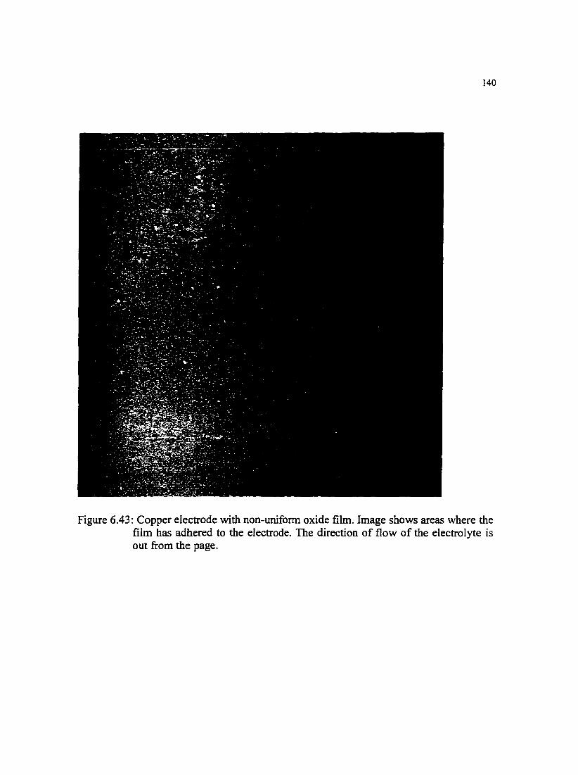
140
Figure 6.43: Copper electrode with non-uniform oxide film. Image shows areas where the film has adhered to the electrode. The direction of flow of the electrolyte is out from the page.
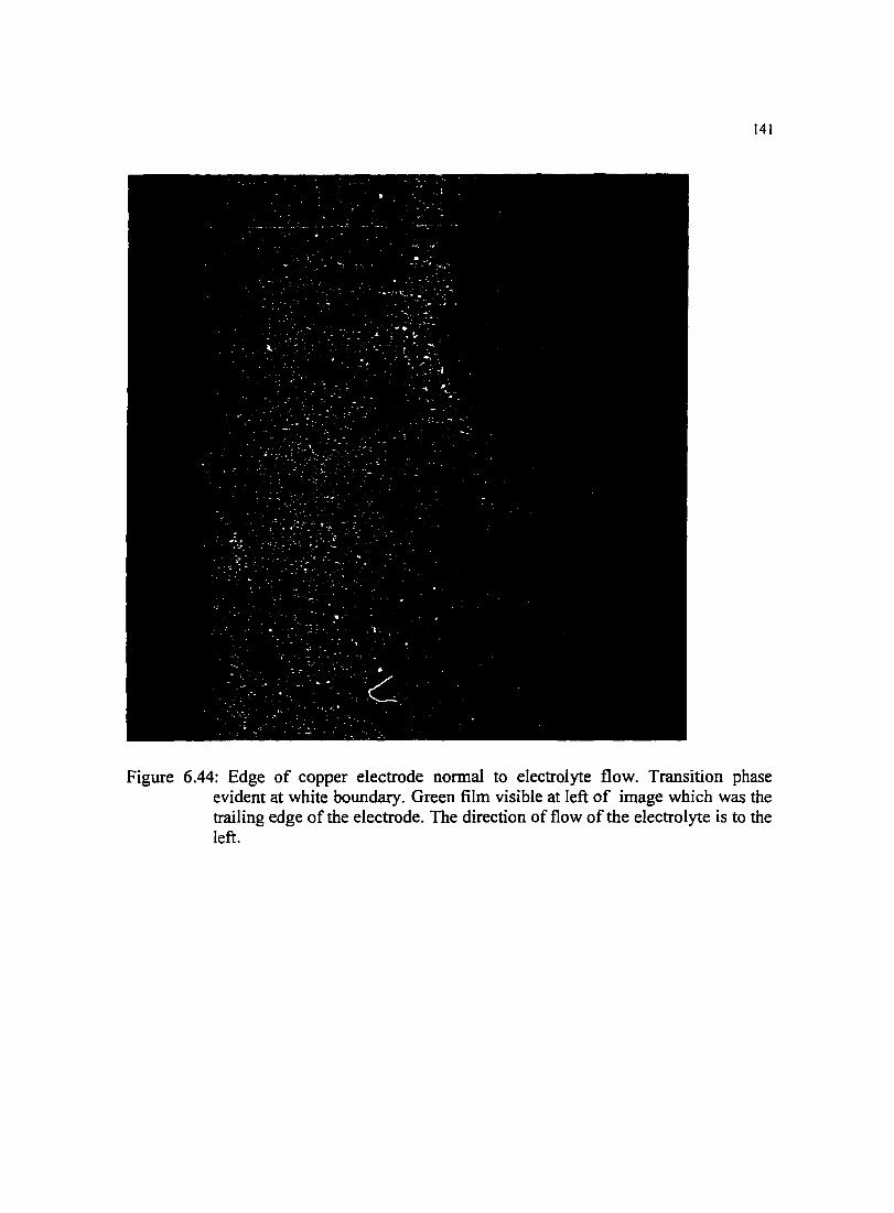
141
Figure 6.44: Edge of copper electrode normal to electrolyte flow. Transition phase evident at white boundary. Green film visible at left of image which was the trailing edge ofthe electrode. The direction of flow of the electrolyte is to the left.
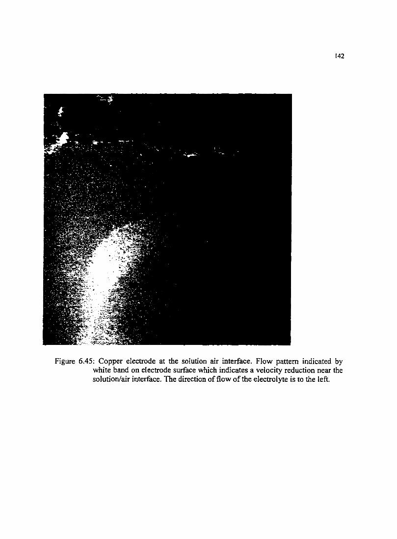
142
Figure 6.45: Copper electrode at the solution air interface. Flow pattern indicated by white band on electrode surface which indicates a velocity reduction near the solution/air interface. The direction of flow of the electrolyte is to the left.

143
Figure 6.46 : Precipitate collected from bottom of recirculation beaker. Blue-green in color, precipitate was collected in a pipette ..

144
Figure 6.47: Precipitate on sample paper, wet.

145
;-~1 ~;,_
t.
Figure 6.48 : Precipitate on sample paper after air drying.
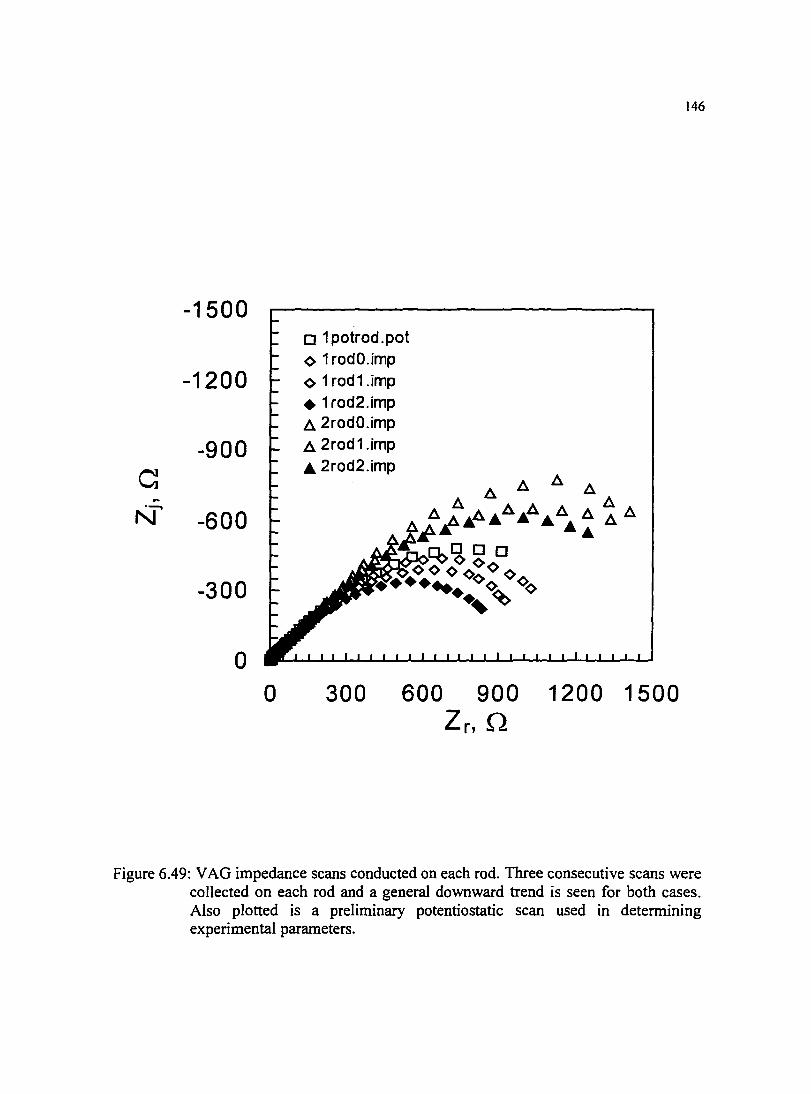
-1500
-1200
-900
-600
-300
0 0
o 1 potrod .pot <> 1 rodO.imp <> 1 rod1.imp
• 1 rod2.imp A 2rodO.imp A 2rod1.imp A. 2rod2.imp
300 600 900 1200 1500 Zr, Q
146
Figure 6.49: VAG impedance scans conducted on each rod. Three consecutive scans were collected on each rod and a general downward trend is seen for both cases. Also plotted is a preliminary potentiostatic scan used in determining experimental parameters.

CHAPTER 7 COMPARISON WITH PAST RESULTS
Efird ( 1977) stated that there is a critical shear stress for different alloys
associated with the mechanical removal of oxide films on the metal surface which leaves
the metal unprotected and susceptible to enhanced corrosion. This work suggests a
different mechanism for enhanced corrosion. This chapter will describe Efird's
experiment, results, and conclusions and compare each to the work conducted for this
project.
Commercially available annealed sheets of copper and four copper alloys were
investigated in a ·•full strength sea water" solution. The test apparatus consisted of a
sample holder with a rectangular cross section designed so sea water could tlow parallel
to the surface of the sample. Flow establishment and disengagement regions were located
up and downstream respectively form the sample to ensure a well developed tlow over
the sample and through the exit orifice. The velocity was mathematically calculated using
the header pressure and orifice size. Velocities for this work ranged from 1.5 m/s to 15
m/s, although the pure copper was tested at lower velocities due to accelerated corrosion
at 1.5 m/s. Temperature and pH control were not implemented; however, the use of fresh
rather than recycled sea water reduced the need for control of the electrolyte pH and
composition. Alteration in corrosion product film, weight loss, thickness loss and
147
148
alteration of metal surface appearance were stated to be used to analyze the samples after
testing.
Thirty day exposures of the samples at different velocities were conducted and the
sample condition was analyzed. Accelerated corrosion was identified by appearance of
the corrosion products and appearance of the metal surface after the corrosion products
were removed. The thickness and mass loss measurements proved to be inconclusive in
determining a value for the critical shear. Examples of images of the cleaned samples
used determine the velocity at which the critical shear was reached are shO\vn in Figure
7 .I (Efird 1977). It should be noted that the onset of enhanced corrosion was consistently
located at the leading edge of the coupon. The resulting values for critical velocity and
shear are given in Table 7.1.
Shear stress as a function of jet velocity for the experimental work conducted here
is presented in Figures 7.2 and 7.3. The curves represent the dimensionless radial position
and the horizontal dashed lines represent the critical shear values reported by Etird for
pure copper and 70130 copper nickel. The vertical dotted lines represent the velocities
investigated in this work; 1.0, 2.0, 4.0, and 6.2 m/s for copper and 2.0 and 6.0 m/s for
70130 copper nickel. Other velocities were also investigated. The velocities of interest
were those that intersected the dimensionless radial position above and belO\v the
reported critical shear for the test material. The velocities that satisfied this criterion for
copper were 1.0 and 2.0 m/s, and 6.0 m/s for 70/30 copper/nickel. If in fact a mechanical
shear removed the oxide layer on the electrode surface, a distinct difference in the
appearance of the electrode surface should be observed past the radial position at which
this shear was achieved. A video image of a copper electrode is presented in Figure 7.4.

149
The copper electrode was immersed in aerated sea water with a velocity of 1.0 m/s for 12
days followed by 2 days at 2.0 m/s. A detailed description ofthe experimental parameters
results is presented in Section 6.5. At a point approximately 1/3 the radius of the
electrode from the center, the reported critical shear was reached with the 2.0 mls jet
velocity. An arrow indicates where one would expect the start of erosion-corrosion.
which would be marked by visible pitting and non-uniformity on the surface. There \vas
no accelerated corrosion on this surface, and the oxide layer was still intact. Examination
of all other electrode surfaces for all runs yielded the same results.
[t is apparent from the images in Figure 7.1 that, m Efird's work. an
increase in the velocity over a certain value caused enhanced corrosion of the electrode
surface. ln contrast, the present work included experiments with shear forces on a copper
electrode twenty times that of the critical shear value reported by Efird and no erosion
corrosion was observed.
Observed in this work was the ability to remove an oxide layer with a small
amplitude potential perturbation (i.e. less that 50 mV~ see section 6.4). [t has also been
shown with this work that salt films resulting from an applied potential can be removed
by fluid flow (see section 6.2). This removal of salt films on specific parts of the
electrode and not on others could further contribute to a potential gradient. Oxygenation
cells are another source of potential gradients which could form when using a channel
type experimental cell. This leads us to conclude that the enhanced corrosion seen by
Efird \Vas not due to a shear removal of an oxide film but to a condition where the tilm
became unstable due to a potential gradient across the electrode surface. The apparatus
used by Efird to conduct experiments did not produce a uniform mass transfer to or away
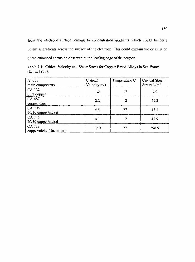
150
from the electrode surface leading to concentration gradients which could facilitate
potential gradients across the surface of the electrode. This could explain the origination
ofthe enhanced corrosion observed at the leading edge ofthe coupon.
Table 7.1: Critical Velocity and Shear Stress for Copper-Based Alloys in Sea Water (Efird. 1977).
Alloy I Critical Temperature C Critical Shear main components Velocity rnls Stress N/m2
CA 122 1.3 17 9.6 pure copper CA687 copper /zinc
2.2 12 19.2
CA 706 4.5 90/10 copper/nickel
27 43.1
CA 715 4.1 70130 copper/nickel
12 47.9
CA 722 12.0 27 296.9 copper/nickel/chromium
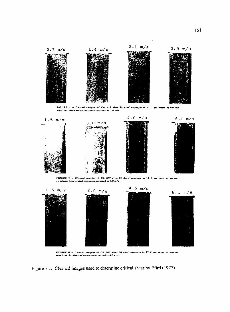
0.7 m/s 1.4 m/s 2.1 m/s 2.9 m/s
FIGURE 4 - Cte~nad samples of CA 122 after 30 days• exposure in 17 C sea water at v•rious velocatres. Accef~r~ted corrosron occurred at 1.4 m/L
1. 5 m/s 3.0 m/s ·f&:-:(ctlr~~-5._..,:· . ~ . ~·
4.6 m/s 6.1 m/s
FIGURE 5 - Clenn~td tamPitK of CA 687 after 30 days"' exposure rn 12 C sea water at various vefocitres. Acaoterated corrosron occurred at 3.0 m/s.
L • S nl/ s 3.0 m/s 4.6 m/s
6.1 m/s
FIGURE 6 - Cleaned samples of CA 706 after 30 days'" exposur~t in 27 C uaa water at various valocitai'!S. Accehtrated corros.on occurred •t 4.6 m/s.
Figure 7.1: C!enncd images used to determine critical shear by Etird ( 1977).
151

-200
-180
-160 C\1
E -140 --z - -120 en
en Q) -100 L-.......
CJ) L- -80 co Q)
-60 ..c CJ)
-40
-20
0 0
. --·-·-- _ _; ·:- ... :-·--;..~ - . ~
.. .. . -. . 70/JO -QJiJNf. . .
---- -:--- --J.-~-. . . . . . .
1 2 3 4
Jet Velocity, m/s
152
5 6 7
Figure 7.2 Shear stress as a function of jet velocity. Curves indicate dimensionless position on the electrode. Horizontal lines represent reported values for critical shear for copper and 70/30 copper nickel (Efird. 1977).

153
-60
-50
N
E -40 --z -C/)
C/) -30 Q)
~ ....., CJ) r/r0=0.8 ~
ro -20 Q)
..c: CJ)
-10
0
0 0.5 1 1.5 2
Jet Velocity, m/s
Figure 7.3: Shear stress as a function of jet velocity. Curves indicate dimensionless position on the electrode. Horizontal lines represent reported values for critical shear for copper and 70/30 copper nickel (Efird. 1977).
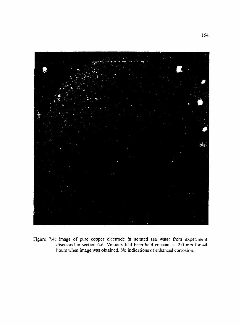
154
Figure 7.4: [mage of pure copper electrode in aerated sea water from experiment discussed in section 6.6. Velocity had been held constant at 2.0 m/s for 44 hours when image was obtained. No indications of enhanced corrosion.
CHAPTERS CONCLUSIONS
This work has shown that a protective oxide film on the surface of a copper
electrode can be irreversibly modified (on the time frame of several days) by an applied
potential perturbation as small as 50 m V. Experiments were conducted which visually
showed the formation and shear removal of salt films under an applied anodic potential.
The current responses to the applied potential supported the visual events occurring on
the electrode surface. The utility of the combination of the impinging jet and video
microscope as a powerful tool in assessing shear-induced corrosion was confirmed in this
work. Shear stresses twenty times the critical shear reported by Efird did not result in
shear removal of oxide films. Concentration gradients driven by localized shear removal
of salt films or oxygenation cell could produce potential gradients across a metal surface
large enough to destabilize protective films resulting in an enhanced corrosion effect.
The extent of aeration of sea water played a key role in the corrosion behavior of
copper. Partially aerated systems were more sensitive to velocity and potential changes
than were those with forced aeration (dissolved 02 = 6.0 and 7.0 ppm respectively). fn
partially aerated sea water. dissolved C02 resulted in a decrease in the local pH near the
electrode causing an equilibrium shift w·hich destabilize some of the tilm components
which were seen in sea water aerated with C02-free air.
155
156
The measurement model was shown to be useful in predicting the polarization
impedance for copper and copper alloys in sea water. The predicted values correlated
well with the experimentally determined values. The measurement model technique was
effective in predicting polarization impedances on systems that were difficult to obtain a
full impedance spectra.
Impedance spectroscopy has been shown to be a useful tool for the non-invasive
evaluation of surface properties of copper and copper based alloys in sea \Vater.
However, in order for this technique to be non-invasive, the perturbation must be small
and the modulation must not change the steady state characteristics. Galvanostatic
regulation is ideally suited for collecting impedance spectra on a corroding metal surface
at the corrosion potential. While conventional galvanostatic measurements can result in
severe swings in potential. the variable amplitude galvanostatic algorithm described here
provides a good means for adjusting the modulation amplitude for current to prevent
large perturbations to the system.
Corrosion potential, impedance spectra, and digital images combined to provide
insight into the mechanisms of corrosion taking place at the electrode surface. The
corrosion potential gave information on the state of the system and the impedance spectra
were useful in determining the resistance to corrosion of the electrode material. The
digital images provided a record on the evolution of the electrode surface as a function of
time. These images indicated whether shear induced preferential corrosion was present.
The effects of flow were evident in cases where a uniform mass transfer condition was
not maintained and when an applied potential caused the formation of thick salt tilms.
which could be removed by shear forces. Results have proven that even after the

157
corrosion potential reached a steady state, oxide films continued to form and evolve on
the electrode surface resulting in an increase in the magnitude of the impedance over
time.

CHAPTER9
SUGGESTIONS FOR FUTURE WORK
More extensive analytical analysis of corrosion products in the form of surface
analysis of the electrode after an experiment or during a phenomena of interest would
assist in further understanding this systems reaction kinetics. Evaluation of corrosion
products in situ could significantly advance this work by supplying empirical data on
possible reactions. Sensors are commercially available which have the capability to
monitor the concentration of species in a flowing stream. In a re-circulating system such
as that of the impinging jet. the implementation of two such sensors. one on the input
stream and one on the effluent stream. would supply a concentration difference which
could be extrapolated back to give information on reactions and reaction rates.
Development of models to describe potential distributions. concentration
gradients. and current distributions of corrosion systems which can be directly applied to
a copper/copper alloy system is currently under way \Vithin our group. This type of model
along with experimental data could lead to predictive techniques for the corrosion rate of
copper and copper alloys in a variety of environments. This information could be used as
\veil to predict the performance of other metals. A data base generated from such a model
would be valuable in the future selection of materials for a specific corrosive
environment.
158

159
Quartz microbalance technology could be applied to this work to determine the
exact amount of corrosion taking place in-situ. One could immediately see the effects of
velocity, light, pH, temperature, and applied potential if the ability to measure mass loss
in siru was available.
Experimentally determined pH near the electrode surface should be investigated
in future work so the stability of corrosion products near the surface could be better
understood (Des louis et al., paper in progress, Moghissi 1993 ).
Further automation of the experimental process to improve the periodicity of data
collection would benefit this project. More frequent collection of digital images of the
surface has become possible even since the inception of this project partially because of
the vast improvements in mass storage devices for personal computers. Large steps
forward have also been taken in the development of faster image acquisition hardware
and software. The image grabber board used to collect digital images for this \vork had a ...... - - -
maximum acquisition rate of approximately one frame in 8.0 seconds. Today. image
acquisition equipment at comparable prices to that paid for the board used in this \vork
are capable of acquiring images at rates of thirty frames per second.
Control of pH, temperature and other variables, which effect the response of this
type system, through the use of a personal computer and a data acquisition interface
would improve the data collection process. Multi-plot displays of all parameters of
interest would assist in determining direction of a given experiment while the experiment
is in progress. The relationship between these parameters could be better analyzed in situ
which could result in the guidance of an experiment to collect the desired data in one

160
experiment where without this interactive adjustment, multiple experiments after post
experiment analysis may be necessary.

APPENDIX A ELECTROCHEMISTRY
Many processes that occur in nature can be studied in the laboratory by supplying
the necessary components of the process of interest. For study of a corroding metal. an
electrochemical cell can be constructed and a vast range of electrochemical techniques
are available to determine corrosion rate, a material's resistance to corrosion. \Vhat and
how many tilms form on the electrode surface. and passivation characteristics.
A metal immersed in an electrolyte is an example of an electrochemical system.
therefore an understanding of a classical electrochemical cell is essential in the study of
copper corrosion. The basic components of a classical electrochemical cell are a cathode.
an anode. and an electrolyte. The cathode and anode, which must be electrically
connected in order to construct a complete circ:.Jit, are often referred to as the counter and
\vorking electrodes respectively. For investigative purposes one or multiple reference
electrodes can be added to the system to provide a standard from which to measure cell
potential.
When a metal comes in contact with an electrolyte, changes on the surface of the
metal occur. Metal atoms disassociate with the surface in the form of positive ions.
cations, resulting in the production of electrons which are free to move through the
metal but are unstable in solution and readily combine with positively charged ions. The
161
162
cation can adsorb to the surface of the metal. In a classical electrochemical cell the free
electron moves through the electrical connection in the form of an electrical current to the
counter electrode where it produces an overall negative charge. Current generated by the
disassociation of electrons in a metal in solution is known as Faradaic current. Mass loss
of a metal in solution is proportional to the Faradaic current, therefore the corrosion rate
can be determined by measuring the Faradaic current.
Measuring current is usually easier in-situ than measuring mass loss. although
both are possible. The cation can desorb into solution and will ditTuse toward the counter
electrode where it will react with available electrons and precipitate or adhere to the
electrode surface. The desorption of the cation into solution constitutes the process of
corrosion on the surface of the working electrode and with this process comes loss of
mass of the working electrode. In order for the corrosion process to readily occur. the
anode and cathode must be composed of different metals. The electromotive force, EMF.
of the metal dictates which electrode will become the cathode and which \Viii become the
anode. The EMF is defined as the difference in potential between two dissimilar metals
immersed in the same electrolyte or otherwise ionically connected (Parker I 994) or that
\Vhich causes a flow of current (Weast I 984 ). The potential difference between a metal
and a reference electrode such as the standard hydrogen electrode, SHE. is known as the
standard electrode potential. Some examples of several standard electrode potentials
versus a SHE are given in Table 2.1 (Bard & Faulkner 1980).
Another example of an electrochemical system is that of two dissimilar metals in
contact with each other and an electrolyte. This situation is known as a galvanic coupling.
Consider copper and zinc metals joined and immersed in an electrolyte. In this system the
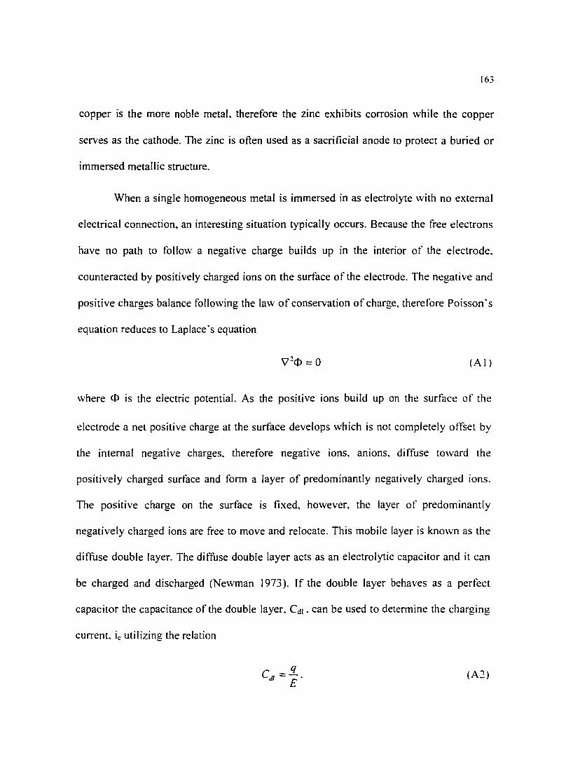
163
copper is the more noble metal, therefore the zinc exhibits corrosion while the copper
serves as the cathode. The zinc is often used as a sacrificial anode to protect a buried or
immersed metallic structure.
When a single homogeneous metal is immersed in as electrolyte with no external
electrical connection, an interesting situation typically occurs. Because the free electrons
have no path to follow a negative charge builds up in the interior of the electrode.
counteracted by positively charged ions on the surface of the electrode. The negative and
positive charges balance following the law of conservation of charge, therefore Poisson· s
equation reduces to Laplace's equation
(A I)
where ci> is the electric potential. As the positive ions build up on the surface of the
electrode a net positive charge at the surface develops which is not completely offset by
the internal negative charges, therefore negative ions, anions, diffuse toward the
positively charged surface and form a layer of predominantly negatively charged ions.
The positive charge on the surface is fixed, however, the layer of predominantly
negatively charged ions are free to move and relocate. This mobile layer is known as the
diffuse double layer. The diffuse double layer acts as an electrolytic capacitor and it can
be charged and discharged (Newman 1973 ). If the double layer behaves as a perfect
capacitor the capacitance of the double layer, Cd1, can be used to determine the charging
current, ic utilizing the relation
C - q dl --.
E (A2)
164
where q is the charge on the double layer and E is the potential across the double layer.
The charging current is then determined using Ohm's law. Under these conditions. no
chemical reaction takes place, therefore no corrosion process are present. If corrosion
processes are present, the total current h, consists of the sum of the charging current and
the Faradaic current (Bard & Faulkner 1980).
(A3)
Copper immersed at the corrosion potential in a solution with oxidizing agents but no
external path for electron flow can still corrode through the establishment of local
cathode and anode sites.
APPENDIXB TIME SUMMARIES
Appendix 8 contains time summaries for experiments presented in Chapter 6.
Information in this section includes times tables corresponding to impedance spectra.
corrosion potential measurements, and video images. The main purpose is to provide
a reference time scale for future work \Vith the data presented.
165

Table B I: Summary of experimental events for data presented in Section 6.3.
Exp, Exq, Exr, flo data Time Frame Information
7/16/96 12:12 experiment start time
hour 0
21 47
557
7/16/96 10:53 7/23/96 13:20
8/8/96 10:32 8/8/96 16:59 8/8/96 17:00
8/13/96 11 :25 8/19/96 9:55
date/time 7/16/96 12:12
7/23/96 13:20 8/8/96 10:30
8/8/96 16:35 8/8/96 17:00
8/8/96 17:25
8/15/96 10:22
8/16/9610:11
to 4.6 29
158
data sets exp exq exr
data sets involved exp, exq, exr, flo
analysis Ecorr. Z Ecorr,Z Ecorr, Z
797 flo Ecorr, Z Rpol
image exp1.tif exp6.tif exp7.tif exp8.tif exp9.tif
exp12.tif exp14.tif
hour -1.32
169.13
671.22 813.72
time. hrs event 0 experiment start
time 169 flow suspended
figure 11 12 13 14 b-4 flow 15 after flow 16 17
7/16/96 17:21 7/18/96 14:57
550 conduct series of Z scans and image grabs until potential application
556 applied potential of >-1.3 volts 557 flow initiated, v =
1m/s 557 resumed standard collection of Ecorr and
z 718 pH change from 8.06 to
controlled 8.24 742 velocity change from 0.6 to 3.4
gal/min
exp3.tif exp5.tif
166
5.15 50.75
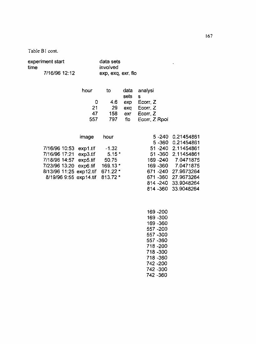
Table 8 I cont.
experiment start time
7/16/96 12:12
7/16/96 10:53 7/16/96 17:21 7/18/96 14:57
hour
0 21 47
557
image
exp1.tif exp3.tif exp5.tif
7/23/96 13:20 exp6.tif 8/13/96 11 :25 exp 12. tif 8/19/96 9:55 exp14.tif
data sets involved exp, exq, exr, flo
to data sets
4.6 exp 29 exq
158 exr 797 flo
hour
-1.32 5.15 *
50.75 169.13 * 671.22 * 813.72*
analysi s Ecorr, Z Ecorr, Z Ecorr, Z Ecorr, Z Rpol
5-240 5-360
51 -240 51 -360
169 -240 169 -360 671 -240 671 -360 814 -240 814 -360
169 -200 169 -300 169 -360 557 -200 557 -300 557 -360 718 -200 718 -300 718 -360 742 -200 742 -300 742 -360
167
0.21454861 0.21454861 2.11454861 2.11454861
7.0471875 7.0471875
27.9673264 27.9673264 33.9048264 33.9048264
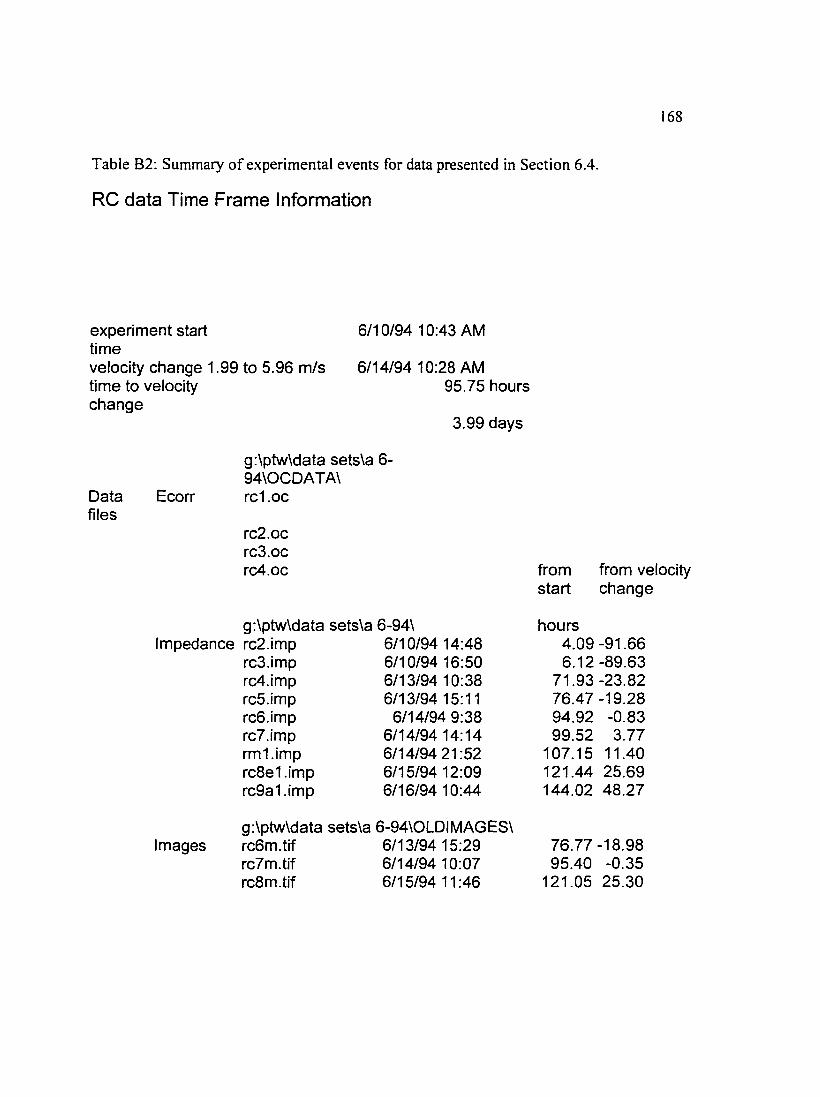
168
Table 82: Summary of experimental events for data presented in Section 6.4.
RC data Time Frame Information
experiment start time
6/1 0/94 10:43 AM
velocity change 1.99 to 5.96 m/s time to velocity
6/14/94 1 0:28 AM 95.75 hours
change
Data files
Ecorr
g:\ptw\data sets\a 6-94\0CDATA\ rc1.oc
rc2.oc rc3.oc rc4.oc
g:\ptw\data sets\a 6-94\
3.99 days
Impedance rc2.imp 6/10/94 14:48 rc3.imp 6/10/94 16:50 rc4.imp 6/13/94 1 0:38 rcS.imp 6/13/94 15:11 rc6.imp 6/14/94 9:38 rc7.imp 6/14/94 14:14 rm1.imp 6/14/94 21:52 rc8e1.imp 6/15/9412:09 rc9a 1.imp 6/16/94 1 0:44
g:\ptw\data sets\a 6-94\0LDIMAGES\ Images rc6m.tif 6/13/94 15:29
rc7m.tif 6/14/94 10:07 rc8m.tif 6/15/94 11:46
from from velocity start change
hours 4.09 -91.66 6.12-89.63
71.93 -23.82 76.47 -19.28 94.92 -0.83 99.52 3.77
107.15 11.40 121.44 25.69 144.02 48.27
76.77-18.98 95.40 -0.35
121.05 25.30

169
Table 83: Summary of experimental events for data presented in Section 6.5.
70130 Cu/Ni data Time Frame Information from start hours
experiment start time 12/6/95 14:22 temperature change 25C to 28C 12/14/95 14:30 192.13
velocity change 1.99 to 5.96 m/s 12/17/95 18:40 268.29
Nl experiment lock up 12/14/95 21:34 Ecorr last point 9/16/96 2:57
g:\ptw\data sets\o 12-95 nickel\
Data files Ecorr ni.oc 12/6/95 14:22 nk.oc 12/17/95 19:28
from from start velocity
g:\ptw\data sets\o 12-95 hours change nickel\
Impedance niOa.imp 12/6/95 15:40 1.29 -267.00 ni13c.imp 12/7/95 14:14 23.86 -244.43 ni19a.imp 12/8/95 18:03 51.68 -216.62 ni22c.imp 12/9/95 16:12 73.83 -194.47 ni25b.imp 12/10/95 16:10 97.79 -170.50 ni28b.imp 12/11/95 19:50 125.46 -142.83 ni30b.imp 12/12/95 14:20 143.96 -124.33 ni33a.imp 12/13/95 16:53 170.51 -97.78 ni35a.imp 12/14/95 17:22 194.99 -73.30 ni36a.imp 12/14/95 20:00 197.63 -70.67 ni36b.imp 12/14/95 20:44 198.36 -69.93 ni36c.imp 12/14/95 21 :34 199.19 -69.10 nkOa.imp 12/17/95 20:46 270.39 2.10 nkOb.imp 12/17/95 21:04 270.69 2.40 nkOc.imp 12/17/95 21:38 271.26 2.97 nk1a.imp 12/17/95 23:46 273.39 5.10 nk1b.imp 12/18/95 0:05 273.71 5.42 nk1 c.imp 12/18/95 0:39 274.28 5.98 nk4a.imp 12/18/95 8:40 282.29 14.00
g:\ptw\data sets\a 6-94\0LDIMAGES\
Images wet.tif 12/6/95 13:36 -0.77 -269.07 nc9.tif 12/10/95 0:30 82.13 -186.17 nc14.tif 12/14/95 23:50 201.46 -66.83

Table 84: Summary of experimental events for data presented in Section 6.6.
Copper (x**.imp) Time Frame Information
experiment start time velocity changes gal/min
0.5 to 1 1 to 2 2 to 3.2
6/21/95 10:13
7/3/95 12:10 7/5/95 14:10 7/6/95 13:55
hours from start
289.95 339.95 363.70
g:\ptw\data sets\m 7-95 hope\81MPDATA\raw data\
Data Ecorr hope.oc 6/21/95 10:13 0.00 files
suz.oc 6/23/95 1 0: 1 0 47.96 x.oc 6/30/95 13:33 219.33
g:\ptw\data sets\m 7-95 hope\81MPDATA\
Impedance x013A.imp 7/2/95 10:02 263.82 x039A.imp 7/5/95 0:12 325.99 x056A.imp 7/6/95 13:39 363.44 x057A.imp 7/6/95 15:29 365.28 x078A.imp 7/11/95 6:30 476.29
g:\ptw\data sets\m 7-95 hope\81MPDATA\
Images h24.tif 7/3/9511:17 289.07 h25.tif 7/3/95 0:30 278.28 h26.tif 7/5/95 9:20 335.12 h27.tif 7/5/95 15:50 341.62 h28.tif 7/6/95 0:58 350.75 h29.tif 717195 10:35 384.37 h30.tif 7/10/95 9:45 455.53
170
from velocity change
289.95 339.95 363.70
REFERENCES
Agarwal. P., Application of lvfeasurement Models to Impedance Spectroscopy. Ph.D. Dissertation, University of Florida, Gainesville, Florida, 1994.
Agarwal, P., Crisalle 0. D., Orazem M. E., and Garcia-Rubio L. H., ''Application of measurement models to impedance spectroscopy. II. Determination of the stochastic contribution to the error structure," Journal of the Electrochemical Society. 142 ( 1995a). 4149-4158.
Agarwal, P .. Moghissi, 0. C., Orazem, M. E., Garcia-Rubio, L. H., ''Application of Measurement Models for Analysis of Impedance Spectra." Corrosion. 49 (I 993a). 278-289.
Agarwal, P., Orazem M. E., Garcfa-Rubio L. H., "Measurement Models for Electrochemical Impedance Spectroscopy I. Demonstration of Applicability," Journal of the Electrochemical Society. 139 ( 1992), 1917-1927.
Agarwal, P., Orazem, M.E., Garcia-Rubio, L.H., "Application of the Kramers-Kronig Relations in Electrochemical Impedance Spectroscopy," Electrochemical Impedance: Analysis and Interpretation, ASTM STP 1188, Philadelphia ( 1993b ), 115-139.
Agarwal P., Orazem M. E., Garcia-Rubio L. H., "Application of Measurement Models to Impedance Spectroscopy. rrr. Evaluation of Consistency with the Kramers-Kronig Relations," Journal ofthe Electrochemical Society. 142 (1995b). 4159-4168.
Alkire, R.C., ''Special Review: Transport Processes in Electrochemical Systems," Chemical Engineering Communications, 38 (1985), 401-413.
Alkire, R., Cangellari, A., "Formation of Salt Films During Anodic Metal Dissolution in the Presence of Flow," Journal of the Electrochemical Society, 130 #6 (I 983 ). I 252-1259.
Alkire, R.C., Perusich, S., "The Effect of Focused Ultrasound on the Electrochemical Passivity of Iron in Sulfuric Acid," Corrosion Science. 23 ( 1983 ), I 121.
Bacarella, A.L., Griess, J.C. "The Anodic Dissolution of Copper in Flowing Sodium Chloride Solutions Between 25° and 175 C0
" Journal ofthe Electrochemical Society. 120 (I 973 ), 459.
171

172
Barcia. O.E., Mattos, O.R., Pebere, N, Tribollet, B. "Mass-Transport Study of the Electrodissolution of Copper in I M Hydrochloric Acid Solution by Impedance:· Journal ofthe Electrochemical Society, 140 #10 (1993), 2825. Bard, A.J., Faulkner, L. R .• Electrochemical Methods Fundamentals and Applications. John Wiley and Sons, Inc. New York ( 1980).
Bianchi, G., Longhi P. '"Copper in Sea-Water, Potential-pH Diagrams," Corrosion Science 13 ( 1973 ). 853-864.
Bird R. B., Stewart W. E .. Lightfoot E. N .• Transport Phenomena. John Wiley and Sons. Inc., New York, ( 1960).
Bjorndahl. W.O., Nobe, K. ''Copper Corrosion in Chloride Media. Effect of Oxygen:· Corrosion 40 #2 ( 1984), 82-87.
Butler, J.A.V. Transactions of the Faraday Society. 19, ( 1924) 729-734.
Chang, Y.C.. Prentice, G., "Calculation of pH Near the Surface of an Electrode Covered with a Porous Film," Electrochimica Acta, 31 #5 ( 1986), 579.
Charriere, E .. ··[mage Analysis of Growing Copper Films in Seawater," Diploma Project 1996-1997, Swiss Federal Institute of Technology, LMCH. Electrochemical Group. University of Florida. Gainesville, Florida ( 1997).
Chin, D-T., Tsang. C-H. '"Mass Transfer to an Impinging Jet Electrode," Journal of the Electrochemical Societv, 125 ( I 978 ), I 46 I.
Cogger. N.D. '"An Introduction to Electrochemical Impedance Measurements:· Technical Report# 006/83, Solartron Instruments, Hampshire, England (I 983 ).
Cogger, N.D. ''The Measurement of Signals from Electrochemical Phenomena:· Technical Report # 0 I 4/84, Solartron Instruments, Hampshire, England (1984 ).
Copson, H.R. '"Effects of Velocity on Corrosion," Corrosion. 16 #2 (1960), 86t.
Dawson, J.L., Shih. C.C., Miller, R.G., Palmer. J.W .• "Inhibitor Evaluations Under Controlled Hydrodynamic Shear," /'vfaterials Pe1formance, 30 (I 991 ). 43.
D'Elia, D, Barcia, O.E., Mattos, O.R., Pebere, N, Tribollet, B. ·'High-Rate Copper Dissolution in Hydrochloric Acid Solution," Journal of the Electrochemical Society. 143 # 3 ( 1996 ). 96 I.
Dhar. H.P., White, R.E., Darby, R .. Cornwell, L.R., Griffin, R.B.. Burnell. G .. ''Corrosion ofCu and Cu-Ni Alloys in 0.5M NaCl and in Synthetic Seawater," Corrosion. 41 ( 1985). 3 I 7.

173
De Sanchez, S.R., Schiffrin, D.J. "The Use of High Speed Rotating Disc Electrodes for the Study of Erosion-Corrosion of Copper Base Alloys in Sea Water," Corrosion Science, 28 #2 (1988), 141
Deslouis, C., Frateur, 0., Maurin, G., Tribollet, B., "Interfacial pH Measurement During the Reduction of Dissolved Oxygen in a Submerged Impinging Jet Cell," paper in progress.
Deslouis, C., Tribollet, B., Mengoli, G., Musiani, M. '"Electrochemical Behavior of Copper in Neutral Aerated Chloride Solution. [. Steady-State Investigation," Journal of Applied Chemistry, 18 ( 1988a), 374.
Deslouis, C., Tribollet, B., Mengoli, G., Musiani, M. ''Electrochemical Behavior of Copper in Neutral Aerated Chloride Solution. II. Impedance Investigation," Journal of Applied Chemistry, 18 ( 1988b), 384.
Diem. C.D., ''The Influence of Velocity on the Corrosion ofCopper in Alkaline Chloride Solutions," Ph.D. Thesis, University ofVirginia, Charlottesville (1990).
Diem, C.B., Orazem, M.E., "Influence of Velocity on Corrosion of Copper in Alkaline Chloride Solutions," Corrosion, 50 #4 (1994), 290.
Etird, K.D. "Potential-pH Diagrams for 90-10 and 70-30 Cu-Ni m Sea Water." Corrosion, 31 #3 (1975) 77.
Efird, K.D. ''Effects of Fluid Dynamics on the Corrosion of Copper-Based Alloys in Sea Water," Corrosion, 33 ( 1977), 3-8.
EG&G Princeton Applied Research. "Model 273 Potentiostat/Galvanostat," Operation Manual ( 1985).
EG&G Princeton Applied Research, "Electrochemical Impedance Measurements: Instrumentation and Techniques," Application Note AC-3, NJ ( 1989).
Esteban. J.M., Hickey, G.S., Orazem, M.E., "The Impinging Jet Electrode: Measurement of the Hydrodynamic Constant and Its Use for Evaluating Film Persistency," Corrosion, 46 #II ( 1990), 896-90 I.
Faita, G., Fiori, G .. Salvadore, D. "Copper Behavior in Acid and Alkaline Brines-1. Kinetics of Anodic Dissoulution in 0.5 M NaCI and Free-Corrosion Rates in the Presence of Oxygen," Corrosion Science, 25 ( 1975), 383.
Fiori, G., Casola, S., Faita, G. "Copper Behavior in Acid and Alkaline Brines. II. Formation of a Protective Layer in Slightly Alkaline 0.5 M NaCI Solutions." Materials Chemistry, 2 ( 1977), 5.

!74
Fontana, M. G., Corrosion Engineering, McGraw-Hill Book Co., New York. ( 1986 ).
Gabrielli, C., '"Identification of Electrochemical Processes by Frequency Response Analysis," Technical Report #004/83, Solartron Instruments, Hampshire, England ( 1980).
Gabrielli, C., "Use and Application of Impedance Techniques," Technical Report, Schlumberger Technologies, Hampshire, England ( 1990).
Gabrielli, C., Huet, F., Keddam, M., ''Investigation of Electrochemical Processes by an Electrochemical Noise Analysis. Theoretical and Experimental Aspects in Potentiostatic Regime," Electrochimica Acta, 31 #8 (1985), 1025.
Gan. E.C., Orazem. M.E. ''A Mathematical Model for the Corrosion of Iron in Sulfuric Acid;' Journal ofthe Electrochemical Society. 134 (1986), 1357.
Gehring. G.A. Jr. "Seawater Corrosion," Materials Pelformance, (September, 1987). 9.
Gilbert, P.T .. '"A Review of Recent Work on Corrosion Behavior of Copper Alloys in Sea Water." 1\tlaterials Peiformance, 21 (1982 ), 4 7.
Gilbert. P.T .. LaQue, F.L. ''Jet Impingement Tests,'' Journal of the Electrochemical Society. 101 #9 ( 1954 ). 448.
Giralt F., Trass 0. "Mass Transfer From Crystalline Surfaces in a Turbulent Impinging Jet Part I. Transfer by Erosion," Canadian Journal of Chemical Engineering. 53 ( 1975). 505.
Goodman, P.O .. ''Effect of Chlorination on Materials for Sea Water Cooling Systems: A Review of Chemical Reactions," British Corrosion Journal. 22 # l ( 1987). 56.
Hack, H.P., Gudas J.P., '"Inhibition of Sulfide-Induced Corrosion by Clean Seawater Preexposure," Report DTNSRDC/SME-79-85, David Taylor Naval Ship Research and Development Center, Annapolis, MD ( 1979).
Hack H.P ., Pickering H. W., ''AC Impedance Study of Cu and Cu-Ni Alloys in Aerated Salt Water;· Journal of the Electrochemical Society. 138 (1991 ), 690.
Hack H.P., Scully J. R. "Galvanic Corrosion Prediction usmg Long- and Short-term Polarization Curves,'' Corrosion. 45 #2 ( 1986), 79.
Hartt, W.H., Culberson, C.H., Smith, S.W. "Calcareous Deposits on Metal Surfaces in Seawater: A Critical Review," Corrosion .40 #II ( 1984), 609
Heitz, E., ··chemo-Mechanical Effects of Flow on Corrosion," Corrosion. 47 ( 1991 ). 135.
175
lves, D.H., Rawson, A.E. "Copper Corrosion III. Electrochemical Theory of General Corrosion," Journal of the Elec!rochemical Society, 109 (1962) 458.
Kauffman, A.M .• "Understanding Electrochemical Cells," Technical Report # 017/85, Solartron Instruments, Hampshire, England ( 1985).
Kendig, M. W., Allen, A. I. , Mansfeld F., "Optimized Collection of AC Impedance Data," Journal ofthe Electrochemical Society. 131 (1984), 935.
Lal. H .• Thirsk. H.R. "The Anodic Behavior of Copper in Neutral and Alkaline Chloride Solution," Journal of the Chemical Society, 3 ( 1953 ), 2638.
LaQue F. L., ··Theoretical Studies and Laboratory Techniques in Sea Water Corrosion Testing Evaluation," Corrosion. 13 (1957). 303t.
LaQue. F., Marine Corrosion: Causes and Prevention. John Wiley and Sons, New York ( 1975).
Law C.G. Jr.. Newman J .... Corrosion of a Rotating Disk in Laminar. Transition. and Fully Developed Turbulent Flow," Journal of the Electrochemical Society. 133 ( 1986 ). 37.
Lee, H.P .• Nobe, K ... Kinetics and Mechanisms of Cu E1ectrodissolution m Chloride Media," Journal of the Electrochemical Society, 133 ( 1986), 2035.
Macdonald.J.R., Impedance Spectroscopy, John Wiley and Sons. Ne\v York ( 1987)
Major Analytical Instrumentation Center (MAIC), Analytical Techniques Handbook. University of Florida. Gainesville ( 1997).
Mansfield, F .. Little, B ... Microbiologically lntluenced Corrosion of Copper-Based Materials Exposed to Natural Seawater," E/ectrochimica Acta, 31 # 12 ( 1992). 2291
Moghissi, O.C.. The Electrochemical Behavior of Copper in Chloride Solutions, PhD dissertation. University of Florida, Gainesville, ( 1993 ).
Newman. J.S .• Electrochemical s_vstems, Prentice Hall, Inc., Englewood Cliffs. NJ (1973).
Orazem. M.E .. Agarwal. P .. Jansen, A.N .. Wojcik, P.T.. and Garcia-Rubio, L.H .. .. Development of Physico-Chemical Models for Electrochemical Impedance Spectroscopy," E/ectrochimica Acta, 38 ( 1993}, 1903-1911.
Orazem. M.E .. Esteban, J.M .. Moghissi, O.C., "Practical Applications of the KramersKronig Relations," Corrosion, 41 (1991},3.

176
Parker, S .• ed., lvfcGran·-Hill Dictionary of Scientific and Technical Terms. 5th ed. McGraw Hill Book Company, New York (1994).
Perry, J.H., Chemical Engineers· Handbook. McGraw Hill Book Company. New York. ( 1963)
Phipps. J. B., Gyory. J. R .• "Transdermal Ion Migration," Advanced Drug Delivery Reviev.:s, 9 (1992) 137-176.
Pourbaix, M.. Atlas of Electrochemical Equilibria in Aqueous Solutions. NACE. Houston. Texas (1974).
Pyun, C.H .• Park, S.M .• ·'In Situ Spectro-electrochemical Studies on Anodic Oxidation of Copper in Alkaline Solution." Journal of the Electrochemical Society, 133 # 1 0 ( 1986 ). 2024-2030.
Scholtz T .• Trass 0. ''Mass Transfer in a Non-uniform Impinging Jet Part I. Stagnation Flow-Velocity and Pressure Distribution," A!ChE Journal. 16 # 1 ( 1970), 82.
Scholtz T., Trass 0. ''Mass Transfer in a Non-uniform Impinging Jet Part II. Boundary Layer Flow-Mass Transfer,·· A!ChE Journal, 16 #I ( 1970b ), 90.
Schlumberger Technologies, ·'1260 Impedance/Gain-Phase Analyzer." Operation Manual. Hampshire, England ( 1993).
Scully J.R., Hack H. P .. Tipton D. G., ·'Effect of Exposure Time on the Polarization Behavior of Marine Alloys Under Flowing and Quiescent Conditions.'' Corrosion. 42 ( 1986 ). 462.
Sethi. V.K .. Wright, I.G., Proceedings of the First International Con.ference on HeatResistant Materials, 439. Sept. ( 1991 ). Fortana, Wisconsin.
Silverman, D.C. "Rotating Cylinder Eiectrode for Velocity Sensitivity Testing.'' Corrosion, 40 ( 1984), 220-226.
Somerscales E.F.C.. Sanatgar H .• '"Hydrodynamic Removal ofCorrosion Products from a Surface.'' British Corrosion Journal, 21 ( 1991 ), 36.
Steele L.R., Geankoplis C. J., ·'Mass Transfer from a Solid Sphere to Water in Highly Turbulent Flow:· AIChE Journal. 5 ( 1959), 178.
Stumm, W., Morgan, J.J., Aquatic Chemistry: An Introduction Emphasizing Chemical Equilibria in Natural Waters, 2nd ed., John Wiley and Sons, Inc. New York ( 1981 ).
Syrett, B.C. ''Erosion Corrosion of Copper-Nickel Alloys in Sea Water and Other Aqueous Environments: A Literature Review," Corrosion, 32 #6 ( 1976) 242.
177
Syrett, B.C., MacDonald, D.O. ''The Validity of Electrochemical Methods for Measuring Corrosion Rates ofCopper-Nickel Alloys in Sea Water," Corrosion, 35 #II ( 1979), 505.
Taylor, A.H. "The Corrosion Behavior of Cu and Naval Brass in 0.5M NaCI Solutions at Ambient Temperature," Journal of the Electrochemical Society. 118 #6 ( 197I ), 854.
Tuthill, A. H. "Guidelines for the Use of Copper Alloys in Seawater," Jvfaterials Performance, ( 1987), 12.
Vahdat N., Newman J., "Corrosion of an Iron Rotating Disk:· Journal of the Electrochemical Society, 120 (1973 ), I682.
Wang. Y.Z .. Beccaria, A.M .• Poggi, G., " The Effect of Temperature on the Corrosion Behavior of a 70/30 Cu-Ni Commercial Alloy in Seawater," Corrosion Science 38 #8. (1994 ). 1277-1288.
Weast. R.C.. ed., CRC Handbook of Chemistry and Physics, 65th ed., The Chemical Rubber Company Press Inc., Boca Raton, Florida ( I984).
White, F.M., Heat Transfer, Addison-Wesley Publishing Company, Reading. Massachusetts ( 1984 ).
Wojcik, P.T., Thermal(v Stimulated Impedance Spectroscopy. Master's Thesis. University of Florida, Gainesville (1992).
Wojcik. P.T., Agarwal, P .. Orazem, M.E., "A Method for Maintaining a Constant Potential Variation During Galvanostatic Regulation of Electrochemical Impedance Measurements," Electrochimica Acta, 41 ( I996), 977-983.
Wojcik, P.T.. Orazem, M.E., "Variable-Amplitude Galvanostatically-Modulated Impedance Spectroscopy as a Tool for Assessing Reactivity at the Corrosion Potential without Distorting the Temporal Evolution ofthe System." Corrosion, in press( 1997a).
Wojcik. P.T., Orazem, M.E., ''Experimental Study of the Erosion-Corrosion of Copper and Copper-Nickel Alloys Using a Submerged Impinging Jet," CORROSION/97. paper 97435 ( I997b ).
Wojcik. P.T.. Orazem, M.E., "Variable Amplitude Galvanostatic (VAG) Modulated Impedance Spectroscopy as a Non-Invasive Tool for Assessing Reactivity at the Corrosion Potential," CORROSION/97, paper 97282 ( 1997c).
Wood, R.J.K. Fry, S.A., "Corrosion of Pure Copper in Flowing Seawater Under Cavitating and Noncavitating Flow Conditions," Journal of Fluids Engineering. 112 ( 1990). 218-224.

178
Wood, R.J.K., Hutton, S.P., Schiffrin, D.J., '"Mass Transfer Effects of Non-Coavitating Seawater on the Corrosion ofCu and 70Cu-30Ni," Corrosion Science. 30 ( 1990), 1177.

179
BIOGRAPIDCAL SKETCH
The author received the Bachelor of Science in Chemical Engineering degree from
the Mississippi State University in August, 1986. He accepted employment with Milliken
and Company as a production supervisor. Seeking a more technical position, he secured
employment with Michelin Tire Corporation in May, 1988, as a process engineer until
returning to graduate school at the University of Florida in August, 1989. The author
received his Master of Science degree majoring in chemical engineering with an emphasis
on solid state physics in May, 1992, and immediately began work on his Ph.D. He will
receive his Ph.D. degree in Chemical Engineering from the University of Florida in
August, 1997, and has secured employment as a senior engineer of technology with Merck
and Company, Inc.

I certify that I have read this study and that in my optmon it conforms to acceptable standards of scholarly presentation and is fully adequate. in scope and quality. as a dissertation for the degree of Doctor of Philosophy.
I certify that I have read this study and that in my optmon it conforms to acceptable standards of scholarly presentation and is fully adequate. in scope and quality. as a dissertation for the degree of Doctor of Philosophy.
Oscar D. Crisalle Associate Professor of Chemical Engineering
I certify that I have read this study and that in my optmon it conforms to acceptable standards of scholarly presentation and is fully adequate, in scope and quality. as a dissertation for the degree of Doctor of Philosophy.
Ranganatha Narayanan Professor of Chemical Engineering
I certify that I have read this study and that in my optmon it conforms to acceptable standards of scholarly presentation and is fully adequate, in scope and quality. as a dissertation for the degree of Doctor of Philosophy.
Associate Engineering
I certify that I have read this study and that in my opm1on it conforms to acceptable standards of scholarly presentation and is fully adequate, in scope and quality. as a dissertation for the degree of Doctor of Philosophy.
~ / ' ' . i ~:;xi ~. -1, ~ :-Ellis D. Verink, Jr. I
Distinguished Service Professor of Material Science and Engineering
This dissertation was submitted to the Graduate Faculty of the College of Engineering and to the Graduate School and was accepted as partial fulfillment of the requirements for the degree of Doctor of Philosophy.
August. 1997 Winfred M. PhillipSY Dean, College of Engineering - - ~
Karen A. Holbrook Dean. Graduate School