information theory and the perception-action cycle

Information Theoryand

The Perception-Action Cycle

Naftali Tishby

Interdisciplinary Center for Neural Computation

The Hebrew University, Jerusalem

Information Beyond ShannonVenice - Italy, December 29-30, 2008,

Perception-Action Cycles

Multiple cycles with

Multiple time scales!


The circular flow of information that takes place betweenthe organism and its environment in the course of a sensory-guidedsequence of behavior towards a goal.

(JM Fuster)

Outline

• Predictive information and the perception-action cycle– A model for the circular flow of information in the cycle(s)– The analogy with Shannon’s Information Theory– The unknown future as the channel input– The future-past channel capacity: Predictive Information

• Two solvable examples– Gambler in a binary world

• Optimal solution: the Past-Future Information Bottleneck

– A linear system in a Gaussian environment• Optimal (Kalman-Ho) dimension reduction in LQR control

• Application to neuroscience– Surprise in Auditory Perception

• Or why do we enjoy music?

Adaptation

Learning

Network-

changes

Development

…

A conceptual framework

The “Environment”: Partially observed, (stationary?) stochastic process

W(t)

past futurenow

xint(t)

a(t)Sensory Input

Actionsw(t)“Organism”

Signal processing

Coding, estimation

Feature extraction

Pattern recognition

Information gathering

…

Decisions

Control / responses

Policies / strategies

Exploration

Environment shaping

…

State

feedback

Metabolic Costs Future Value

Internal state

futurerewards

sensing costs

We must simplify …

(…hopefully not oversimplify…)

Internal Representations

NOW

The Environment: stationary stochastic process


PAST FUTURE

Internal

Representation


PAST FUTURE

X Y

T

(Optimal) Internal Representationswe like to think probabilistically

X

T

Y

YXP ,

XTP | TYP |

• Environment: P(X,Y)

• Internal representation: P(T|X), P(Y|T)

Actuators

(“encoders”)

Sensors

(“decoders”)

Information Theoretic view of


The environment

Sensing Cost Actions Value

Unknown

Future

(channel

input)

Predictive

Channel

[partially]

observed

Past

(channel

output)

The organism

rewards

r(a,w+)costs

e(w-,x)

W+W

-

p(W-|W+)

p

ax

u

t x=f(x,u)

y=g(x,u)

yDynamical

system

state-space

Actuators

(“encoders”)

Sensors

(“decoders”)

Simpler

Perception-Action Cycle

The environment

Sensing Cost =

I(W-;X)

Action Value

I(X;W+)

Unknown

Future

(channel

input)

Predictive

Channel

[partially]

observed

Past

(channel

output)

The organism

internal

memory

rewards

r(a,w+)costs

e(w-,x)

W+W

-

p(W-|W+)

p

a

xu y

(no dynamics)

cost-

e(w-,x)= coding

rate

Reward -

r(a,w+)= prediction

rate

Optimum: The Information Bottleneck optimal decoders/predictors

X

T

Y

YXI ;

XTI ; YTI ;

• Environment: I(X;Y) – predictive information

• Internal representation: I(T;X) , I(T;Y) - compression & prediction

(Optimal) Internal Representationsand we want a computational principle…

X

T

Y

YXI ;

XTI ; YTI ;

Model Quantifiers:

• Complexity (“cost”): I (T;X)

• Predictive Info (“value”): I(T;Y)

Optimality Trade-off:

• minimize complexity

• maximize predictive-info

model

past future

(Optimal) Internal Representationsand a computational principle…

• Environment: I(X;Y) – predictive information

• Internal representation: I(T;X) , I(T;Y) - compression & prediction

A simple example:

The compulsive gambler in a binary world

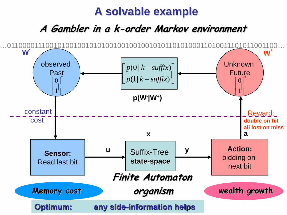
Action:

bidding on

next bit

Sensor:

Read last bit

A solvable example

Memory cost wealth growth

Suffix-Tree state-space

Reward:double on hit

all lost on miss

constant

cost

ax

u y

A Gambler in a k-order Markov environment

1

1

Unknown

Future

observed

Past

W+W

-

p(W-|W+)

(0 | )

(1| )

p k suffix

p k suffix

*

0

1

*0

1

Finite Automaton

organism

Optimum: any side-information helps

…011000011100101001001010100100100100101011010100011010011101011001100…

The optimal compulsive gambler

1

1

kth-order Markov environment

Memory + reading Cost

Value:

Wealth growth

Unknown

Future

observed

Past

X: PFSA organism (Probabilistic Finite State Automata)

W+W

-

p(W-|W+)

0

1

0

1

Optimum: proportional bidding with IB predictive information

Cost:

I(past;X)

E log Value =

I(X;future)

The Predictive Channel

Predictive Information: The Capacity of the Future-Past Channel

(with Bialek and Nemenman, 2001)

– Estimate PT(W(-),W(+)) : T- past-future distribution

W(t)

past futureW(-)- T-window

t=0

W(+)- T-window

( , )

( | )[ ] log

( )past future

T Tfuture past

pred Tfuture

p W W

p W WI T

p W

Logarithmic growth for finite dimensional processes

• Finite parameter processes (e.g. Markov chains)

• Similar to stochastic complexity (MDL)

dim( )( ) log

2predI T T

Power law growth

• Such fast growth is a signature of infinite dimensional processes

• Power laws emerges in cases where the interactions/correlations have long range

( ) 1predI T T

But WHAT - in the past - is predictive ?

W(t)


t=0

W(+)- T-window

– Find the “relevant part” of the past w.r.t. future…

Solve: Min Z I(W(-);Z) - I(W(+);Z) for all >0

T- past-future information curve: ITF(IT

P)

– IFuture(IPast) = limT→∞ ITF(IT

P)

The predictive capacity has multiple scales

W(t)


t=0

W(+)- T-window

The environment’s Predictive Information boundsthe cycle’s efficiency and the Perception-Action Capacity

.

IFuture

Ipast

IT1

F (IT1P)

IT2

F (IT2P)

IT3

F (IT3P)

The limit is always the concave

envelope of increasing time-windows

Information Curves

A simple illustration

2,,

18,18,...,2,1

YBAy

Xx

YXP ,

2 4 6 8 10 12 14 16 18

A

B

2 4 6 8 10 12 14 16 180

0.2

0.4

0.6

0.8

12 4 6 8 10 12 14 16 18

A

B

2 4 6 8 10 12 14 16 180

0.2

0.4

0.6

0.8

1

P (

Y=

B|X

)

0 1 2 3 40

0.05

0.1

0.15

0.2

I(T;X)

I(T

;Y)

Info Curve

X

T

P(T|X)

2 4 6 8 10 12 14 16 18

2

4

6

8

10

12

14

16

18

2 4 6 8 10 12 14 16 180

0.2

0.4

0.6

0.8

1

X

Predictions


XHXTIXT ;,P

(„B

‟|X

)

(most complex) (perfect copy) (perfect predictions)

0 1 2 3 40

0.05

0.1

0.15

0.2

I(T;X)

I(T

;Y)

Info Curve

X

T

P(T|X)

2 4 6 8 10 12 14 16 18

2

4

6

8

10

12

14

16

18

2 4 6 8 10 12 14 16 180

0.2

0.4

0.6

0.8

1

X

Predictions


bit3; XTIP

(„B

‟|X

)

0 1 2 3 40

0.05

0.1

0.15

0.2

I(T;X)

I(T

;Y)

Info Curve

X

T

P(T|X)

2 4 6 8 10 12 14 16 18

2

4

6

8

10

12

14

16

18

2 4 6 8 10 12 14 16 180

0.2

0.4

0.6

0.8

1

X

Predictions


bit2; XTIP

(„B

‟|X

)

0 1 2 3 40

0.05

0.1

0.15

0.2

I(T;X)

I(T

;Y)

Info Curve

X

T

P(T|X)

2 4 6 8 10 12 14 16 18

2

4

6

8

10

12

14

16

18

2 4 6 8 10 12 14 16 180

0.2

0.4

0.6

0.8

1

X

Predictions


bit1; XTIP

(„B

‟|X

)

0 1 2 3 40

0.05

0.1

0.15

0.2

I(T;X)

I(T

;Y)

Info Curve

X

T

P(T|X)

2 4 6 8 10 12 14 16 18

2

4

6

8

10

12

14

16

18

2 4 6 8 10 12 14 16 180

0.2

0.4

0.6

0.8

1

X

Predictions


bit5.0; XTIP

(„B

‟|X

)

0 1 2 3 40

0.05

0.1

0.15

0.2

I(T;X)

I(T

;Y)

Info Curve

X

T

P(T|X)

2 4 6 8 10 12 14 16 18

2

4

6

8

10

12

14

16

18

2 4 6 8 10 12 14 16 180

0.2

0.4

0.6

0.8

1

X

Predictions


bit0; XTIP

(„B

‟|X

)

Application to neuroscience:

Auditory cortex encodes surprise

(or why do we enjoy music?)

(with Israel Nelken and Jonathan Rubin, Shlomo Dubnov)

The predictive bottleneck

Correlation with the model, along the information-curve

0 0.5 1 1.5 2 2.5 3 3.5 4 4.50

0.05

0.1

0.15

0.2

0.25

0.58

0.6

0.62

History length = 17

Complexity

Pre

dic

tive I

nfo

0 0.33 0.67 1 1.33 1.67 2 2.330

0.05

0.1

0.15

0.2

Model Complexity (bits)

Pre

dic

tive

Po

we

r (b

its)

012345

123456

012 345

123456

012345

123456

012345

12345

0 1 2 3 4 5

123

0 1 2 3 4 5

12

0 1 2 3 4 5

12

Information curve showing the optimal predictive information

(surprise) as a function of the complexity of the internal model

(memory bits) for the next-tone prediction of oddball sequences using

a memory duration of 5 tones back.

The physiological surprise

Quantifying the complexity of neural representations

Left: scatter plots of the neural responses to either „A‟ (blue) or „B‟ (red) and the surprise values calculated for a specific

model. Dots mark the mean response at a given surprise level, and the error-bars represent 25 and 75 percentile of the data.

Right: (1) PSTH for stimulus „A‟, each row is the averaged PSTH corresponding to a single point in the scatter-plot, sorted

from low to high surprise level. (2) PSTH for stimulus „B‟. (3) Correlations for „A‟ (as explained before). (4) Correlations for „B‟.

The PSTH plots help to see what part of signal is correlated with the surprise. For instance the onset seems pretty constant

(and absent in the responses to „B‟), where the sustained part seems to be very correlated with the surprise.

(1)

(2)

(3)

(4)

Cortical representation of (optimal) auditory surprise

Summary

- This model extends old results on optimal gambling to a muchmore general optimal value-cost tradeoff with long sensing-decision-action sequences

- Crucial quantities are the “environment’s predictive capacity” and the “perception-action-capacity”.

- While obviously still rudimentary, the model provides new ways for analyzing neuroscience data and new insights on motorcontrol and deficiencies.

- The Perception-Action Cycles have an intriguing analogy with Shannon’s model of communication, which suggests asymptotic bounds on the optimal cycle’s efficiency

Many Thanks to…

• Bill Bialek• Amir Globerson• Ilya Nemenman• Eli Nelken• Jonathan Rubin• Gal Chechik• Shlomo Dubnov• Ohad Shamir• Naama Parush• Felix Creutzig• Roi Weiss

information theory and the perception-action cycle

Documents