information paradox under the scope of ads/cft …
TRANSCRIPT
Imperial College London
Department of Physics
Theoretical Physics Group
Information paradox under the scope ofAdS/CFT correspondence
Author:
Panagiotis Giannadakis
Supervisor:
Prof. Toby Wiseman
Submitted in partial fulfilment of the requirements for the degree of Masterof Science of Imperial College London
MSc Quantum Fields and Fundamental Forces
London, September 25, 2020

Abstract
This thesis project is submitted for the Master of Science of Imperial College London Msc
Quantum Fields and Fundamental Forces and it a review about Hawking imformation
paradox and some recent developments concerning it from the perspective of AdS/CFT
correspondence. The aim of the project is to present what the information paradox is
and where it comes from, also how a black hole can be seen as a quantum mechanical
object evolving in a unitary way. Then our interest will focus on a recent development
which offers a way to recover the Page curve of the entropy of Hawking radiation which is
an important tool to determine if a black hole as a quantum system evolves in a unitary
manner, by considering a black hole system in 2-dimensions living in an asymptotically
AdS2 spacetime.

Acknowledgements
With the submission of this dissertation another fascinating academic cycle is now closing.
At this point I need to thank my supervisor Pr. Toby Wiseman for his his assistance
throughout the duration of this project and for his thorough explanations to many of my
questions and also for the courses of QFT annd QED. Furthermore, I would like to thank
the rest of the academic staff in Theory Group for everything they have taught us during
this year. Of course, I also need to pay a special tribute to my QFFF course mates who
made this year unique even under the craziest circumstances of COVID19 pandemic and
especially to Sergi Sirera, Ethan Schreyer, Joe Willsher, Jordi Rafecas, Nick Kolev and
Johannes Rosok. I wish them all, best of luck. Finally, I would like to thank my family
and my friends in Greece for their support in every level during this year.

Contents
Introduction 7
1 Hawking radiation 8
1.1 Review of black hole Thermodynamics . . . . . . . . . . . . . . . . . . . . 8
1.2 Quantum Field Theory in curved spacetime . . . . . . . . . . . . . . . . . 13
1.3 Particle creation in curved spacetime . . . . . . . . . . . . . . . . . . . . . 16
1.4 Black hole evaporation . . . . . . . . . . . . . . . . . . . . . . . . . . . . . 23
2 Black Hole Information 25
2.1 Pure and mixed states in Quantum Mechanics . . . . . . . . . . . . . . . . 25
2.2 Entanglement and Entropy . . . . . . . . . . . . . . . . . . . . . . . . . . . 26
2.2.1 Entanglement entropy . . . . . . . . . . . . . . . . . . . . . . . . . 27
2.2.2 Coarse-grained entropy . . . . . . . . . . . . . . . . . . . . . . . . . 28
2.3 Seeing a black hole as a quantum system . . . . . . . . . . . . . . . . . . . 29
2.4 Hawking Information Paradox . . . . . . . . . . . . . . . . . . . . . . . . . 30
2.5 Unitary evolution and the Page curve . . . . . . . . . . . . . . . . . . . . . 36
3 AdS/CFT correspondence 41
3.1 Conformal field theories (CFTs) . . . . . . . . . . . . . . . . . . . . . . . . 42
3.1.1 Conformal group . . . . . . . . . . . . . . . . . . . . . . . . . . . . 42
3.1.2 Correlators . . . . . . . . . . . . . . . . . . . . . . . . . . . . . . . 44
3.1.3 Stress energy tensor and central charge . . . . . . . . . . . . . . . . 46
3.2 Anti de Sitter spacetime . . . . . . . . . . . . . . . . . . . . . . . . . . . . 46
3.3 AdS/CFT dictionary . . . . . . . . . . . . . . . . . . . . . . . . . . . . . . 50
3.4 Holographic entanglement entropy . . . . . . . . . . . . . . . . . . . . . . . 51
3.4.1 The Ryu-Takayanagi formula . . . . . . . . . . . . . . . . . . . . . 51
3.4.2 Heuristic proof of RT formula . . . . . . . . . . . . . . . . . . . . . 52
3.4.3 Proof of Strong Subadditivity . . . . . . . . . . . . . . . . . . . . . 54
2

CONTENTS
3.4.4 The Hubeny-Rangamani-Takayanagi formula . . . . . . . . . . . . . 54
3.5 Examples of calculation of entanglement entropy . . . . . . . . . . . . . . . 56
3.5.1 Holographic dual of CFT2 on an interval R1,1 . . . . . . . . . . . . 56
3.5.2 Holographic dual of CFT2 on R× S1 . . . . . . . . . . . . . . . . . 57
3.5.3 Entanglement entropy of CFT2 at finite temperature . . . . . . . . 58
4 Holographic derivation of the Page curve 60
4.1 The fine-grained entropy of a gravitational system . . . . . . . . . . . . . . 60
4.2 Gravity coupled to holographic matter . . . . . . . . . . . . . . . . . . . . 62
4.2.1 2-dimensional gravity coupled to CFT2 . . . . . . . . . . . . . . . . 63
4.2.2 Black hole coupled to holographic bath . . . . . . . . . . . . . . . . 66
4.2.3 The entanglement entropy of the 2-dimensional theory . . . . . . . 67
4.3 Entanglement wedges for an evaporating black hole . . . . . . . . . . . . . 69
4.3.1 Early times . . . . . . . . . . . . . . . . . . . . . . . . . . . . . . . 69
4.3.2 Late times . . . . . . . . . . . . . . . . . . . . . . . . . . . . . . . . 71
4.3.3 Reproducing the Page curve . . . . . . . . . . . . . . . . . . . . . . 74
Conclusions 75
Bibliography 75
3

Introduction
Black holes are some of the most interesting macroscopic objects we have ever detected
in the universe and also their very existence has given a lot of food for thought in modern
theoretical physics, in many different perspectives. During the 60s and 70s there was
a productive and thorough theoretical study of black holes from classical perspective,
where it had been realized that their mechanics obey some laws and behave like thermo-
dynamic objects [1, 2] with temperature T = ~κ2πkB
(Hawking temperature), where κ is the
surface gravity of the black hole, and entropy given by Bekenstein-Hawking expression
SBH = Area4GN~ which is proportional to the area of the event horizon.
Those quantities took actual physical meaning when in 1974 Hawking [3] proved that
considering a quantum field theory in a dynamical curved spacetime of a spherically sym-
metric black hole, an observer at causal infinity J + detects a constant flow of particles
emitted by the black hole. He also proved that the spectrum of this radiation follows
the Planck distribution of black body’s spectrum with temperature equal to the Hawk-
ing temperature above. This phenomenon now is called Hawking radiation and is the
first endeavour of unifying a theory of dynamical spacetime and quantum field theory
in a semiclassical approximation where spacetime itself is a classical geometric entity of
General Relativity but is also supplied with quantum fields. Hawking radiation itself is a
result of the fact that in a curved spacetime there is not a preferred way to define positive
or negative modes in a field theory and this implies, in terms of multiparticle states, that
the vacuum of a region next to black hole’s event horizon does not seem empty at all,
by an observer at infinity but full of multipartilcle states instead. Also microscopically it
can be seen as the creation of entangled particle pairs where one is outgoing and escapes
at infinity whereas its partner falls into the black hole, so the full Hilbert space consists
of the subspace related to the outgoing states and the subsystem concerning the interior
and can be written as H = Hint ⊗Hrad .
4

CONTENTS
Then the main implication of Hawking radiation was Information paradox [4] which is
perhaps one of the most astonishing and subtle problems of theoretical physics come forth
during the 20th century. Information paradox emerged soon after Hawking first published
his famous paper about Hawking radiation when he argued that due to the radiation a
black hole of mass M0 loses mass and eventually shrinks up to the point that after time
tevap ∼ M30 completely evaporates leaving behind only thermal radiation. Therefore, all
information concerning the initial quantum state of the black hole is lost forever. In other
words, if we start with some collapsing matter to form a black hole described by a pure
quantum state |ψ〉BH then after evaporation is completed we will have a thermal state of
Hawking radiation. But the later does not contain any information about former black
hole’s degrees of freedom and moreover, it is not a pure state anymore. This means that
from a pure quantum state we end up with a mixed thermal state, something which can-
not be acquired by a unitary time evolution operator whose action on a pure state should
give a pure state. This seems to violate one of key assumptions of quantum mechanics
and formulates the paradox.
Of course the paradox is a paradox only under the assumption of the black hole be-
ing an ordinary quantum system with Area4GN~ degrees of freedom, dependent on the area of
the horizon. During the 90s works by Preskill and Suskind [5, 6] gave a new perspective
to the black hole realization by introducing the so-called holographic principle which re-
duces the study of a black hole as a d-dimensional gravitational system to d-1-dimensional
holographic quantum theory. Then in 1997 the discovery of AdS/CFT correspondence
became the best studied example of a holographic duality. The hypothesis mentioned
above is widely accepted today especially from the perspective of string theory and is
considered as a main basis for studying the information paradox. Subsequently, whatever
the solution for the paradox may be it must respect the unitarity of the black hole as an
ordinary quantum system.
An implication of unitarity is that the time evolution of the entanglement or von Neumann
entropy of Hawking radiation SR = −TrBH(ρR log ρR) (where we trace out the black hole
degrees of freedom and ρR the density operator concerning the state of radiation) should
follow the Page curve [7, 8, 9]. Initially, just after black hole’s formation, the entanglement
entropy of radiation is very small compared to Bekenstein entropy (practically zero) and
should increase, until it reaches a maximum value equal to Bekenstein entropy (where the
degrees of freedom of radiation are equal to black hole’s ones) at Page time t ∼ 0.6tevap.
5

CONTENTS
Then it starts decreasing until the final evaporation where it takes zero value. The use-
fulness of Page curve is determined by the fact that its successful derivation by certain
gravity theory would indicate that this theory would respect unitarity and therefore, infor-
mation paradox seems to be resolved. However, we have to emphasize the that Page curve
on its own can tell us nothing sufficient about the final quantum state after evaporation
is completed. Notice that Hawking himself strongly disagreed with unitarity and argued
that the entanglement entropy entropy of Hawking radiation should increase monoton-
ically from whence the black hole is created and settles down until it finally evaporates [4].
A major difficulty in order to recover the Page curve is that we do not have yet a full, con-
sistent theory of quantum gravity which means that it is not known what the exact state
of the system radiation-black may be. Therefore, it is not easy to calculate the entropy by
direct calculation using its definition. Nevertheless, in the last 15 years there has been sig-
nificant development in this field in terms of AdS/CFT correspondence. It turns out that
the entanglement entropy of a gravitational system coupled to a conformal field theory
living in d-dimensions is associated with finding a minimal (or rather extremal) surface in
d+ 1-dimensional dual bulk theory in AdSd+1 spacetime. The first formula was proposed
by Ryu and Takyanagi [10] and then it has been extended by various authors [11, 12, 13].
The most recent realization is that the entanglement entropy of a gravitational system
of an evaporating black hole is given by a minimal quantum extremal surface [13]. This
is a surface that extremizes the generalized entropy (Bekenstein+von Neumann entropy
of quantum fields in black hole region) and if there are more than one such surfaces the
minimal one determines the entropy. The benefit of Ryu-Takyanagi prescription is that
the problem of entropy becomes a geometrical problem which in general is easier to be
solved.
Recent works [14, 15] show that for an evaporating black hole at early times the ex-
tremal surface is the trivial and thus the initial increase in entropy of radiation happens
due to the quantum fields contribution, as the Hawking radiation starts to escape to in-
finity. If the early state of the black is pure then the whole interior region belongs to the
entanglement region or the entanglement wedge of the black hole. Past the Page time
there is a new quantum extremal surface which is located behind the event horizon and
at Page time there is a phase transition where the surface behind the horizon becomes
minimal. Then most of black holes’s interior is now excluded from the entanglement
wedge of the black hole and the as the black hole continues to evaporate and shrink the
6

CONTENTS
corresponding area shrinks too and thus the entanglement entropy of the black hole.
A new proposal in 2019 [16] is that the Page curve of Hawking radiation can be recovered
by considering a gravity theory in 2-dimensions with holographic matter, i.e. a confor-
mal field theory which has a dual bulk theory in 3-dimensions coupled to a 2-dimensional
holographic bath. The main innovative idea is that finding appropriate quantum extremal
surfaces in this case is equivalent with Ryu-Takyanagi (or rather its cavariant) prescrip-
tion and it follows that the extremal surfaces of radiation and black hole coincide and
thus it follows the same rise before the Page time and then the same decrease recovering
the full Page curve for radiation entropy. An important point is that this prescription
gives rise to a disconnected entanglement wedge of radiation which consists of two region:
one would represent Hawking result from the radiation escaped at infinity but also there
is a second region which covers most of the interior at late times beneath the quantum
extremal surface. This region is called quantum extremal island and it is a region in
the gravitational theory where matter is entangled with the external quantum system.
Another point which is worth noticing, is that this island, which in 2-dimensional realiza-
tion is disconnected with the rest of the entanglement wedge, in the dual 3-dimensional
description is actually connected via the extra dimension.
The aim of this thesis project is to discuss the above topics. The thesis is organized
in four chapters. We start our discussion with a review of black hole thermodynamics and
also a thorough presentation of Hawking radiation considering that unfortunately, due
to the COVID19 pandemic was not covered in QFFF class. The next chapter is about
the entanglement entropy in quantum mechanical systems and we analyze information
paradox. Then follows a discussion about what AdS/CFT correspondence is and some of
its main conclusions especially its usefulness in calculating entanglement entropies with
Ryu/Takyanagi prescription. Finally, in the last chapter we are going to review the paper
[16] and see how the Page curve can be obtained by holography. The standard conven-
tions are ηµν = diag(−1, 1, 1, 1) and in the standard natural units c = ~ = kB = GN = 1,
although we mostly write down the Newton’s constant.
7

Chapter 1
Hawking radiation
1.1 Review of black hole Thermodynamics
In this chapter we will try to review some topics concerning the black hole mechanics and
thermodynamics and then we will see that black holes are actually thermal bodies with
non zero temperature and therefore they emit Hawking radiation. This chapter is mainly
based on the original papers from 70s’ of Hawking and Beckenstein [1, 3] as well as lecture
notes by F. Dowker [17], J. Gauntlett [18] (Imperial College London),H. Reall [19] P.K.
Townsend [20] (University of Cambridge). Many details for black hole thermodynamics
are omitted for the sake of simplicity. The goal is to give a main idea that the black holes
are thermodynamic objects and where the Hawking radiation comes from.
Uniqueness theorems
Black holes are some of the most remarkable results provided by General Relativity (GR).
The basic way of the formation of a black hole is by the stellar collapse of a supermassive
star during a supernovae explosion. Soon after its formation it is classically thought the
black hole settle down to a "time independent"1, stationary state.
By stationary state we mean a state where the black hole spacetime is asymptotically
flat [17] and it admits a Killing vector k which is timelike near causal infinity. If a black
hole with mass M is rotating with angular momentum J = Ma (in that context a is the
angular momentum per unit mass) and also has electric charge Q then this black hole is
described by Kerr-Neuman solution (1965) [21] of the Einstein’s equations in the vacuum
1In reality this happens very fast
8

1.1. REVIEW OF BLACK HOLE THERMODYNAMICS
of Einstein-Maxwell theory2 with metric in Boyer-Lindquist coordinates (with GN = 1)
ds2 = −(∆− a2sin2θ
Σ
)dt2 +
Σ
∆dr2 − 2
asin2θ
Σ(r2 + a2 −∆)dtdφ
+Σdθ2 +((r2 + a2)2 −∆a2sin2θ
Σ
)sin2θdφ2 (1.1)
where Σ = r2 +a2cos2θ and ∆ = r2−2Mr+Q2 +a2 with a corresponding electromagnetic
potential expressed as
A = (At, Ar, Aθ, Aφ) =(Qr
Σ, 0, 0,−Qarsinθ
Σ
)(1.2)
This is the most general solution for charged rotating black holes. Moreover, for a = 0,
Q = 0 we recover the spherically symmetric solution i.e. the usual Schwarzschild metric
whereas if only Q = 0 then the metric (1.1) reduces to the Kerr solution.
The Kerr-Neumann solution is axisymmetric which means that it admits another Killing
vector m that is spacelike near causal infinity and all orbits of m are closed [20]. In local
coordinates this Killing vector can be expressed as m = ∂φ.
Between 1967 and 1975 were proved some very powerful uniqueness theorems by Israel
(1967)[22], Carter (1971) [23], Hawking (1973) [24] and Robinson (1975) [25] which lead
to the conclusion that the unique stationary asymptotically flat black hole solution of the
vacuum Einstein-Maxwell theory is the Kerr-Neumann with three parameter family M ,
J , Q. Those theorems indicate that no matter how the black hole was initially formed,
the equilibrium state will be Kerr-Neumann and the information about its formation has
been lost either by falling into the black hole or by radiation.
The conclusions of those theorems is the so-called no-hair theorem "the black holes have
no hair" first quoted by J. Wheeler. The no hair theorem seems presumably correct at
least in the classical description of a black hole. In other words one black hole can be
fully described by a family of just three classical parameters mass, angular momentum
and electric charge.
We carry on by giving a few definitions and theorems, for more details we refer the
2The vacuum of gravity theory coupled with Electromagnetism in classical regime.
9

1.1. REVIEW OF BLACK HOLE THERMODYNAMICS
reader to Black holes Lecture Notes by Dr. P.K. Townsend [20]. Let S(x) be a smooth
function of some spacetime coordinates xµ. Then we can obtain a family of hypersurfaces
with normal vector field to those hypersurfaces
l = f(x)(gµν∂νS)∂
∂xµ(1.3)
where f an arbitrary non zero function.
Definition: A hypersurface N for which l2 = 0 is called null hypersurface.
A null hypersurface has the property that since for a normal on it l2 = l · l = 0 any normal
on that surface is also tangent vector.
Definition: A null hypersurface N is called Killing horizon if there is a Killing vector
field ξ which is normal to the null hypersurface N .
There is also an interesting theorem by Hawking (1972) [26]
Theorem: For an analytic, asymptotically flat vacuum (or Einstein-Maxwell vacuum)
spacetime of a black hole the future event horizon H is also a Killing horizon. By the
definition of the Killing horizon we conclude that
ξ = fl (1.4)
Subsequently we have for ξ that
ξµ∇µξν = flµ∇µ(flν) = flνlµ∇µf = κξν (1.5)
where
κ = ξµ∂µln|f | (1.6)
this quantity is called surface gravity and it is called so because is constant on the horizon3
and its physical meaning is just the force which must be exerted at infinity in order to
maintain a unit mass on the horizon.
Now we have not said anything about the stress energy tensor of Einstein’s equations. We
want to consider only physical matter which respects the causal structure of spacetime.
Therefore, there is a motivation to define some energy conditions the stress energy tensor
must respect.
Dominant energy condition: The stress energy tensor Tµν satisfies the dominant en-
3This is indeed the zeroth law of black hole thermodynamics
10
1.1. REVIEW OF BLACK HOLE THERMODYNAMICS
ergy condition if for all future-directed timelike vector fields v, the vector field
j(v) = −vµT νµ∂ν (1.7)
called ”energy-momentum current” is future directed causal.
Weak energy condition: It is a less restrictive condition which states that
Tµνvµvν ≥ 0 (1.8)
for any timelike vector v. Note that the weak energy condition is actually implied by the
dominant which is the physically important one.
Black hole thermodynamics
We are now proceeding to the laws of black hole thermodynamics. In 1973 a paper by
Bardeen, Carter and Hawking [1] was published concerning the ”The laws of black hole
thermodynamics”. The idea of this article was that as in classical thermodynamics there
are four fundamental laws which determine the state of a classical thermodynamic system,
for the black holes also exist four laws which correspond to the thermodynamic ones.
We now present those laws.
Oth Law
The surface gravity κ is constant on the future event horizon H+ of a stationary black
hole spacetime obeying the dominant energy condition.
This law transcends the 0th law of thermodynamics which states that the temperature
T throughout a physical thermodynamic system in thermal equilibrium is uniform across
the system.
1st Law
The 1st Law of black hole thermodynamics implies the conservation of energy by express-
ing how the three fundamental classical quantities M , J and Q change if a black hole
initially characterized by those three quantities is perturbed to a new stationary state
characterized by M + dM , J + dJ , Q+ dQ. The mathematical expression of the 1st Law
is
dM =1
8πκdA+ ΩHdJ + ΦHdQ (1.9)
11

1.1. REVIEW OF BLACK HOLE THERMODYNAMICS
where here ΩH is the angular velocity of the black hole, ΦH is the surface electric potential
and A is the Area of the horizon. The thermodynamic analog is the usual first law of
thermodynamics which is expressed as dE = TdS +∑
i µidNi.
Here again the first law has a similar structure with the thermodynamic analog. Again
the quantity κ8π
is like the temperature and the area A is the analog of entropy.
2nd Law (Area Law)
This law demands that the Area of the event horizon can never decrease so
δA ≥ 0 (1.10)
That implies that if we start for example with two stationary black holes which eventually
merge and form a new black hole, the Area of the new black hole must be greater than
the sum of the surfaces of the initial ones.
Again it is evident the analog of entropy from the second law of thermodynamics which
states that δS ≥ 0 is the surface A. But the second law of black hole thermodynamics
is slightly stronger than the corresponding traditional second thermodynamic law. Clas-
sically we can transfer entropy from one system to another, under the requirement that
the total entropy of the universe does not decrease. However in the case of black holes it
is not possible to do this with the area, from one black hole to another since black holes
cannot bifurcate. Hence, the second law requires that the area of each black hole should
not decrease individually.
3rd Law
It is impossible to reduce surface gravity κ to zero by a physical process. The correspond-
ing 3rd thermodynamic law states that we cannot achieve zero temperature by a physical
process.
Bear in mind that initially the authors of this paper [1] perceived those quantities as
ones which just correspond to the original thermodynamic but they do not have exact
physical correspondence but rather purely mathematical. The primary idea had been that
the black holes have zero temperature, since nothing can escape from them, and therefore
do not radiate nor possess physical entropy. This idea of course changed swiftly after
Hawking published his famous paper on black hole radiation [3].
Nontheless, a year later in 1974 Bekenstein [2] argued that the second law of thermody-
namics would be violated if black holes had no entropy, since one could throw an arbitrary
12

1.2. QUANTUM FIELD THEORY IN CURVED SPACETIME
large amount of matter into a black hole and thus reduce the total entropy of the universe
according to an observer who stands outside of the hole horizon, but this is a disaster be-
cause we demand that the classical thermodynamic laws are still valid. Thus, he proposed
a generalized second Law which affirms that the total entropy of the entire universe must
not decrease and by total entropy or generalized entropy otherwise we mean the sum of
the entropy of the external universe and the entropy of the black hole which should be
proportional to the area A. In other words defining Sgen = Sext + SBH
δSgen = δ(Sext + SBH) ≥ 0 (1.11)
Then in the same year Hawking derived the result that black holes in reality are ther-
mal bodies and they radiate with black body temperature (expressed with all constants
GN , ~, kB)
T =~κ
2πkB(1.12)
and the black hole entropy is
SBH =A
4GN~(1.13)
Which is called Bekenstein-Hawking entropy4. Meanwhile the quantity G~ has dimension
[l]2 and so we can define the Planck length lP =√G~ to express thw entropy as SBH = A
4l2P.
Also, if we work in natural units ~ = kB = 1 then we have the term in first law of black
hole thermodynamics analogous with the classical thermodynamic temperature. Thus we
realize that this analogy was not just a bare coincidence but a one to one correspondence
or rather a physical unification [17].
1.2 Quantum Field Theory in curved spacetime
Our goal now is to show and elaborate the result of Hawking (1974) [3]. We begin by
generalizing the quantum field theory from the flat Minckowski space to an arbitrary
curved spacetime with metric gµν . We focus on the real, scalar field φ with Lagrangian
L =1
2gµν∇µφ∇νφ−
1
2m2φ2 (1.14)
4We will simply call it from now and on Bekenstein entropy or simply just black hole coarse grainedentropy see chapter 2. Note also that Bekenstein did not have in his mind that the entropy of the blackhole had the expression named after him but rather a more general one.
13

1.2. QUANTUM FIELD THEORY IN CURVED SPACETIME
The equation of motion is the Klein-Gordon equation in curved spacetime expressed as
∇µ∇µφ−m2φ = 0 (1.15)
where φ = φ(t, ~x) and the conjugate momentum defined as
π =∂L
∂(∇0φ)=√−gφ (1.16)
As always for the quantization of the system we consider the usual equal time commutation
relations:
[φ(t, ~x), φ(t, ~y)] = 0 (1.17)
[π(t, ~x), π(t, ~y)] = 0 (1.18)
[φ(t, ~x), π(t, ~y)] =i√−g
δ3(~x− ~y) (1.19)
We assume a globally hyperbolic spacetime i.e. one which has a Cauchy surface. Defini-
tion: A partial Cauchy surface Σ is a hypersurface where no past and future inextendible
causal curve intersects more than once. when a manifold admits a Cauchy surface, it can
be foliated by a family of Cauchy surfaces.
The significance of Cauchy surfaces lies in the fact that once a Cauchy surface has been
chosen along with some initial data on it, the corresponding solution to the equations of
motion is completely determined on the entire spacetime [17]. Consequently, everything
can be determined from a set of initial data.
We will define a new inner product as between two (generally complex) functions
(f, g) = i
∫Σ
dΣ√−g(f1∇µg
∗ − g∇µf∗) (1.20)
and for two real scalar fields φ1, φ2 will be
(φ1, φ2) = i
∫Σ
dΣ√−g(φ1∇µφ2 − φ2∇µφ1)
For Klein-Gordon solutions this inner product does not depend on the choice of the Cauchy
slice. To show that let’s take two arbitrary Cauchy slices Σ,Σ′ then
(φ1, φ2)Σ′−(φ1, φ2)Σ = i
∫Σ′dΣ√−g(φ1∇µφ2−φ2∇µφ1)− i
∫Σ
dΣ√−g(φ1∇µφ2−φ2∇µφ1)
14

1.2. QUANTUM FIELD THEORY IN CURVED SPACETIME
= i
∫∂S
dS√−g(φ1∇µφ2 − φ2∇µφ1) = i
∫S
∇µ(φ1∇µφ2 − φ2∇µφ1)
where in the last step we used Gauss ’ theorem. Now note that
∇µ(φ1∇µφ2−φ2∇µφ1) = ∇µφ1∇µφ2+φ1∇2φ2−∇2φ1φ2−∇µφ1∇µφ2 = φ1m2φ2−m2φ1φ2 = 0
and therefore
(φ1, φ2)Σ′ = (φ1, φ2)Σ
When we do the quantization of the scalar field in Minckowski spacetime we expand the
field in basis of positive and negative frequencies e±ipx which is Lorentz invariant and so
respects the symmetries of Minckowski space. Nonetheless, in a curved spacetime there
is not such a thing as the Lorentz invariance. Thus, it is not so easy to define a basis of
positive and negative frequencies whatsoever, because a using a different basis the new
observer would not necessarily see the same positive or negative frequencies. In fact, even
worse, there is not a preferred choice of basis.
So first of all we consider an orthonormal basis ψi [18] such that
(ψi, ψj) = δij
(ψi, ψ∗j ) = 0 (1.21)
(ψ∗i , ψ∗j ) = −δij
where here the indices i, j have similar role as the momentum in the flat Minckowski space
and they are continuous indices but we emphasize they do not represent the physical
momentum because on Minkowski space we assume the on-shell condition whereas here
not. Now the quantized field can be expressed by expanding in that basis as
φ(x) =∑i
aiψi(x) + a†iψ∗i (x) (1.22)
and we require that the creation and annihilation operators obey the usual commutation
relations of quantum field theory [ai, a†j] = δij. The basis of the Hilbert space is the
vacuum |0〉 with ai |0〉 = 0 and the multiparticle states constructed by the action of
creation operator on the vacuum. Nevertheless, the above condition does not fix the
space of all solutions. In a region of an asymptotically flat spacetime the basis functions
ψi should contain only positive frequencies with respect to the time coordinate and would
15

1.3. PARTICLE CREATION IN CURVED SPACETIME
remain positive for all observers whereas for a general curved spacetime there is nothing
which demands this anymore. So if we start, for instance, with our initial basis which can
be seen as an initial flat region followed by a region of curved spacetime and then again
by a third flat region, the vacuum of the final region will not be the same as the one of
the initial one because the basis of the first region will not be identical to the one in third
region while both contain positive frequencies. Subsequently, the action of annihilation
operator of the first region will not generally give zero if it acts on the vacuum of the
third. This rather obscure statement can be interpreted as a particle creation of the scalar
field by the gravitational field itself.
Now if we take another basis ψ′i we can expand ψ′ with respect to the previous basis as
ψ′i =∑i
Aijψj +Bijψ∗j (1.23)
The new basis satisfies the orthonormality relations if
AA† −BB† = I (1.24)
ABT −BAT = 0 (1.25)
The A,B coefficients satisfying the above conditions are called Bogoliugov coefficients.
Now if we want to invert (1.23) we would have
ψj =∑k
A′jkψ′k +B′jkψ
′∗k (1.26)
with
A′ = A†, B′ = −BT (1.27)
and the requirement that A′, B′ obey the same conditions as A, B do gives that
A†A−BTB∗ = I (1.28)
A†B −BTA∗ = 0 (1.29)
1.3 Particle creation in curved spacetime
Now in order to elaborate this result of particle creation we consider a globally hyperbolic
spacetime which is time dependent and is stationary at early times, then becomes non-
stationary and at late times becomes again stationary [19]. We can denote this spacetime
16

1.3. PARTICLE CREATION IN CURVED SPACETIME
asM = M−∪M0∪M+ where -,0 and + for early, intermediate and late times respectively.
So we have for that spacetime
• Region 1: M− which corresponds to the spacetime at very early times before the
formation of the black hole and it is asymptotically flat. We take this region at J −.
• Region 2: M0 which is the curved non-stationary spacetime around the black hole
after its formation.
• Region 3: M+ at late times after gravitational collapse and very far from the black
hole. Hence this spacetime is asymptotically flat. We then take that region in J +.
At early and late times as we said the spacetime is stationary and there is indeed a pre-
ferred basis of positive frequencies (which are well defined) subspace. Label this preferred
choice of positive frequency eigenfunctions as ui with respect to a stationary future-
directed time translation Killing vector field k [18]. We also choose them to obey the
standard orthonormality relations. Since this Killing vector generates a symmetry, the
Lie derivative of the field φ with respect to k, Lkφ must be a solution of Klein-Gordon
equation provided φ is a solution itself and therefore, we deduce that k maps solutions of
Klein-Gordon to some other solutions. Furthermore, the Lie derivative Lk is an antiher-
mitian operator, a fact which indicates that we can choose a basis of positive frequencies
with imaginary eigenvalues. Lkui = −iωiui with ωi > 0
If there is a positive mode in the first region passing through the curved specetime region
of the black hole, then an observer in the third region may see a superposition of positive
and negative modes. This can be viewed as the fact that the gravitational field in region
2 is a new potential V which can alter the original quantum state as a perturbation and
therefore, in region 3 a superposition of positive and negative frequencies may be revealed.
Having considered the above we are now able to expand the field with respect to the
preferred positive frequency eigenfunctions, u±i which are solutions of Klein-Gordon in
M±. Notice also that for the intermediate region the field cannot be expressed in such a
basis since the spacetime is not stationary.
Hence we have in M±
φ(x) =∑i
a±i u±i (x) + a±†i u
∗±i (x)
17

1.3. PARTICLE CREATION IN CURVED SPACETIME
We also saw that since the inner product defined by (1.20) does not depend on the choice
of the Cauchy surface hence the matrix product of A, B will be same. So, expressing the
field as
φ =∑i
a−i u−i + a−†i u
∗−i
=∑i
(a−i∑j
(Aiju+j +Biju
∗+j ) + a−†i
∑j
(A∗iju∗+j +Biju
+j ))
=∑i,j
(a−i Aij + a−†i B∗ij)u
+i + h.c. =
∑i
(a+i u
+i + a+†
i u∗+i )
we conclude that the Bogoliugov transformation of the creation-annihilation operators are
a+i =
∑j
(a−i Aij + a−†i B∗ij) (1.30)
We define now the number operator of the field in regions M± respectively as
N± = a±†i a±i (1.31)
What would one see if they act with number operator N+i on the vacuum of region M−
denoted as |0−〉?Assuming the corresponding vacuum expectation value one can notice that
〈0−|N+i |0−〉 = 〈0−| a+†
i a+i |0−〉 =
∑j,k
〈0−| (a−k Bki)(a−†j B
∗ji) |0−〉
=∑j,k
〈0−| a−k a−†j |0−〉BkiB
†ij = (B†B)ii = Tr(B†B)
So the expected number of particles is
〈N+i 〉 = Tr(B†B) (1.32)
5 and since B†B is positive by its definition it turns out that this expectation value van-
ishes if and only if B vanishes. Non zero B implies particle creation which escapes from
the black hole at infinity. Our aim for now and on is to discover the form of this Bogoli-
ugov coefficient Bij. We will eventually see that this radiation turns out to be thermal.
Let’s have a look over that amazing result calculated by Hawking in 1973 which eventu-
ally was named after him, Hawking radiation and it’s the first essential result of coupling
5here there is no summation over the i index
18

1.3. PARTICLE CREATION IN CURVED SPACETIME
between the gravity of GR and the quantum field theory.
For the purpose of the calculation we are going to consider a spherically symmetric so-
lution of the Einstein equation, the Schwarzschild metric, which illustrates a non rotat-
ing uncharged black hole, and a massless scalar field φ. The Schwarzschild metric in
4-dimensions is
ds2 = −(
1− 2M
r
)dt2 +
dr2
1− 2Mr
+ r2dΩ22 =
(1− 2M
r
)(−dt2 + dr2
∗) + r2dΩ22 (1.33)
using tortoise coordinate r∗ for which
dr2
1− 2Mr
=(
1− 2M
r
)dr2∗ ⇒ r∗ = r + 2M log
∣∣∣ r2M− 1∣∣∣
and it can be also expressed by the advanced and retarded coordinates u = t − r∗ andv = t+ r∗ as
ds2 = −(
1− 2M
r
)(−dudv) + r2dΩ2
2 (1.34)
the tortoise coordinate r∗ for large r, r∗ ≈ r and so we can use it in the regions 1 and 3
instead of r.
In the spherically symmetric metric the Klein-Gordon equation of (1.15) can be rewritten
using the formula from differential geometry
∇µ∇µ =1√−g
∂µ(√−ggµν∂ν) (1.35)
and writing φ = φ(t, r∗, θ, φ). Expanding in spherical harmonics φ(t, r∗, θ, φ) = e−iωtRl(r∗)Ylm(θ, φ)
we have for the radial part Rl(r∗) that it solves the equation
(∂2r∗ + ω2 − Vl(r∗))Rl(r∗) (1.36)
where
Vl(r∗) =(
1− 2M
r
)[ l(l + 1)
r2+
2M
r3
](1.37)
19

1.3. PARTICLE CREATION IN CURVED SPACETIME
This is the potential barrier we mentioned before.
Near J ± the solutions are just plane waves. Specifically on J −
flmω′(out) =1
(2πω′)1/2e−iω
′uYlmr
(outgoing) (1.38)
flmω′(in) =1
(2πω′)1/2e−iω
′vYlmr
(ingoing) (1.39)
and on J +
glmω(out) =1
(2πω)1/2e−iωu
Ylmr
(outgoing) (1.40)
glmω(in) =1
(2πω)1/2e−iωv
Ylmr
(ingoing) (1.41)
A positive mode gω at J + is given by (1.40) and we would like to investigate its past, in
other words how it is related with the ingoing mode fω′ at J − given by (1.38). Note that
in reality plane waves such as gω at J + are completely delocalized [18], but despite that,
we still can construct wave packets on J + which are localized around an ω0 and u0.
The mode gω can be expressed as an integral over the incoming frequencies ω′ at J − as
gω =
∫ ∞0
dω′(Aωω′fω′ +Bωω′f∗ω′) (1.42)
We assume that gω, following a null cosmic line γ, arrives at J + in infinite time. So going
backwards in time from J + the wave gω at some point was close to the event horizon
H+ and eventually meets the dynamical potential barrier. Then part of the wave gRω will
be reflected by the barrier to J − and will not experience the curved geometry at all.
Therefore, it ends up to J −. The other part gTω of the wave transmits through the barrier
and thus enters the time dependent geometry and ends up as a mixture of positive and
negative modes on J −.
In fact, since we are interested in a wave packet localized and peaked at late times where
u0 >> 1 and finite frequency ω0, the wave packet will be peaked at a very high frequency
as it enters the collapsing matter due to the gravitational blueshift [17]. Because of that
we are allowed to use geometric optics approximation [27] where gω = A(x)eiS(x) and A(x)
is has very small variation in comparison with S(x). Subsequently, the Klein-Gordon gives
∇µS∇µS = 0 which implies that surfaces of constant phase are null. These surfaces seem
to accumulate close to the horizon.
20

1.3. PARTICLE CREATION IN CURVED SPACETIME
Consider now a null geodesic congruence which contains those hypersurfaces and also
the event horizon which is at S = ∞. Take also its tangent vector l and also a future
directed null vector n, generator of the Killing horizon H+ at a point x which is directed
inwards and has nl = −1. This is a connecting vector because −εn (ε > 0) connects
a point on the event horizon with a nearby null hypersurface of constant phase. The
spherical symmetry of the problem allows us to take the vector n with vanishing angular
components.
The mode gω going backwards following the null geodesic γ starts at some point with
coordinate u = u0 at J + and hits J − at some v = v0. The generator of H+ can be
extended to the past so that it hits J − at some point with coordinate, without loss of
generality, v = 0 6. Then v0 < 0. Near the horizon the Kruskal coordinates (U = −e−κu,V = eκv) define an affine distance along n and we can use them in order to measure
the distance between γ and γH . Then outside the horizon the null geodesic is located at
U = −cε. By the definition of U itself we deduce that u = − 1κ
log(−U) and so at late
times γ will have coordinate u = − 1κ
log(cε) with c positive constant.
Furthermore, since γ is outgoing null geodesic with phase gω ∼ eiωu we take [20]
−iωu =iω
κlog(cε) (1.43)
with c > 0 constant and then at J − l, n can be expressed in u, v coordinates as l ∼ ∂u,
n ∼ D−1∂v where D again a positive constant. Thus on J − the proper distance between
γ and γH is −D−1ε and the phase iωκ
log(−cDv). Therefore, the transmitted wave on J −
ignoring the nornalization and a constant phase is given by
gTω ∼ eiωκ
log(−v) v > 0 (1.44)
and it vanishes for v ≤ 0.
Now in order to find the coefficients Aωω′ and Bωω′ of (1.42) consider the Fourier trans-
formation of the gTω
gω(−ω′) =
∫ +∞
−∞dveiω
′vgTω (v) =
∫ 0
−∞dveiω
′v+ iωκ
log(−v) (1.45)
6since the spacetime is invariant in translations
21

1.3. PARTICLE CREATION IN CURVED SPACETIME
Now for gTω (−ω′) it can be proven [17, 20] that
gTω (−ω′) = −eπωκ gTω (ω′), ω′ > 0 (1.46)
Having this result now we take the inverse Fourier transformation
gTω (v) =
∫ +∞
−∞
dω′
2πe−iω
′vgTω (ω′) =
∫ +∞
0
dω′
2πe−iω
′vgTω (ω′) +
∫ +∞
0
dω′
2πe+iω′vgTω (−ω′)
=
∫ ∞0
dω′Nω′fω′(v)gωT (ω′) +
∫ ∞0
dω′N∗ω′f∗ω′(v)gω
T (−ω′)
where Nω′ , N∗ω′ are normalization factors. Hence we have for positive ω, ω′
Aωω′ = Nω′ gTω (ω)
Bωω′ = N∗ω′ gTω (−ω)
and thereby using the result of (1.46) we finally find
|Bωω′ | = e−πωκ |Aωω′| (1.47)
Now finally the normalization of the transmitted wave is given by the defined inner product
Γω = (gTω , gTω ) =
∫ω′
∫ω′′
(Aωω′fω′ +Bωω′f∗ω′ , Aωω′′fω′′ +B∗ωω′′) =
∫ω′
(|Aωω′|2 − |Bωω′ |2)
= (e2πωκ − 1)
∫ω′|Bωω′ |2 = (e
2πωκ − 1)(BB†)ωω
and thus finally
〈N+ω 〉 = Tr(BB†) =
Γω
e2πωκ − 1
(1.48)
But this is exactly a black body radiation with a factor Γω which can be seen as an absorp-
tion cross section and most importantly with temprtature T = κ2π
which is the Hawking
temperature. The result is remarkable, it shows that expectation value of the number of
particles counted at J + follows a thermal radiation distribution and it is a continuous
flow of thermal particles whose temperature depends only on the surface gravity. For
Schwarzschild black hole κ = 4M so using the thermodynamic definition of temperaturedSdE
= 1T, identifying E = M and taking the condition S(E = 0) = 0 we recover the
Beckenstein result of entropy S = A4(ignoring some constants).
22

1.4. BLACK HOLE EVAPORATION
But what exactly is that rather peculiar Hawking radiation?
Well it is a result coming from quantum field theory in a gravitational field of a black
hole. A good intuitive but of course not accurate picture is the following. The vacuum of
the quantum field theory is characterized by constant activity which means spontaneous
creation of pairs of particle-antiparticle which very quickly annihilate in order to main-
tain the total energy of the vacuum zero. However in the environment of the black hole
close to the event horizon it is possible that a pair be created close to the horizon and a
particle escapes at J + while its partner falls into the black hole. In order the total energy
of the vacuum is maintained ,since the escaping particle has positive energy, the infalling
particle must have negative energy. That means this is a virtual particle which falls into
the black hole and reduces its mass. In other words the Hawking radiation makes the
black hole to evaporate. This process is a great milestone of modern physics as it brings
forth a difficult problem The information paradox for which we are going to discuss in
the next chapter.
1.4 Black hole evaporation
The result of Hawking is that at infinity we have a constant flow of particles. This implies
that energy flows from the black hole to infinity and thus this energy must be taken away
from its mass. This process is called Black hole evaporation and it leads to the eventual
disappearance of the black hole. Considering a black hole as black body at Hawking
temperature we can calculate the power of that radiation classically from Steffan’s law
dE
dt= −σAT 4
H (1.49)
and since E = M , A ∼ M and also TH ∼ 1M
for Schwarzschild black hole, we deduce
that dMdt
= − aM2 , where a is a constant and therefore the evaporation time tevap = γM3
0 .
Here γ = 13a
and M0 is the initial mass of the black hole after gravitational collapse.
The lifetime of a solar mass black hole is then estimated at 1064 years, compared to the
universe age around 1013 years!!!
We need to emphasize here that this calculation is purely classical and thus contains no
information about the geometry and its backreaction because of the evaporation process
but still remains an accurate approximation for the loss of energy while it is radiated away
23

1.4. BLACK HOLE EVAPORATION
in a slow rate i.e. dMdt<< 1. Nevertheless, this picture does not remain equally accurate
during the late stages of evaporation because as its mass becomes smaller and smaller
the emission rate increases drastically and when black hole’s mass becomes comparable
to Planck mass this rate become enormous. In order to be able to conclude more accurate
results for those late times we need a theory of quantum gravity.
24

Chapter 2
Black Hole Information
2.1 Pure and mixed states in Quantum Mechanics
In Quantum mechanics any quantum system is described by a state |ψ〉 which is a vector
that lives on a Hilbert spaceH. Every ideal meaurement on the quantum system is related
to a projection operator Πi in the way that the probability of a measurement to give an i
result on the quantum system, can be found by the action of the projection operator Πi
on the state |ψ〉 [28]
Pr(i) = |Πi |ψ〉 |2 〈ψ|Π†iΠi |ψ〉 (2.1)
A projection operator is one that Π2i = Πi. We are going to define now a new object
called the desnity operator ρ (or density matrix) defined as ρ = |ψ〉 〈ψ|.Using the above definition of density operator and expanding in an appropriate basis we
can write the probability of a measurement as
Pr(i) =∑n
〈ψ|n〉 〈n|Π†iΠi |ψ〉 =∑n
〈n|Π†iΠi |ψ〉 〈ψ| |n〉 (2.2)
=∑n
〈n|Π†iΠiρ |n〉 = Tr(Π†iΠiρ) (2.3)
and similarly if we want to compute an expectation value of an operator A we find that
〈ψ|A |ψ〉 = Tr(Aρ) (2.4)
Consequently, we are deduce that the density operator is a useful and important object in
quantum mechanics and within it, all the information of the quantum system is included.
25

2.2. ENTANGLEMENT AND ENTROPY
A pure state is defined as one where the density operator can be written in the form
ρ = |ψ〉 〈ψ|. By the definition of ρ we easily see that Trρ = 〈ψ|ψ〉 = 1 and also Trρ2 =
〈ψ|ψ〉2 = 1. On the other hand, a mixed state is one that has a density operator ρ =∑i pi |ψi〉 〈ψi| and more than one of pi is non zero, this corresponds to a state which is
written as |ψ〉 =∑
i
√pi |ψi〉 where |ψi〉 is an orthonormal basis and pi ≥ 0. In this case
again if we take the trace of ρ we have Trρ =∑
i pi = 1 but on the other hand if we take
the Trρ2 we will have Trρ2 6= 1 because ρ2 =∑
i p2i |ψi〉 〈ψI | which means
Trρ2 =∑i
(pi(pi − 1) + pi) =∑i
pi(pi − 1) + 1 < 1
[28, 29] and therefore the way to check whether a state is mixed is to take the trace of
ρ2 and see if it is 1 or less. The density operator also has the good properties that it is
hermitian and also positive definite.
2.2 Entanglement and Entropy
If we consider now a bipartite quantum system with a density matrix ρ living on a Hilbert
space H = HA⊗HB, this system consists of two subsystems A and B with a complete and
orthonormal basis say |n〉A, |m〉B respectively and also density matrix ρ = ρAB [28, 29].
An observer who has access only to one system, without loss of generality assume A, what
they can measure comes from a density matrix regarding the subsystem A, ρA. We can
define the reduced density operators for each subsystem as ρA = TrBρ and ρB = TrAρ. For
such a bipartite system a state will be pure if it is factorizable and thus if it can be written
as a tensor product of two states of each subsystem i.e |ψ〉 = |n〉A⊗|m〉B ≡ |n,m〉AB. On
the other hand, if a state cannot be expressed as such a tensor product the state is mixed
and we say that the two subsystems are entangled which means they are associated to
one another.
If we have a factorizable state of a bipartite system then the reduced density matrices
describe pure states as well. For example, if we take a state |ψ〉AB = |0, 0〉AB then
ρ = ρAB = |0, 0〉 〈0, 0| and so
ρA = TrBρ = |0〉A 〈0|A
whisch again describes a pure state. So any factorizable states are not entangled.
However, if we have a non factorizable state in general, the reduced density matrices will
26

2.2. ENTANGLEMENT AND ENTROPY
not describe pure states.
As an example we consider a Bell state [28, 30] which obviously is not factorizable and
thus
|ψ〉AB =1√2
(|0, 1〉+ |1, 0〉) (2.5)
Here the density matrix has a form
ρ = |ψ〉AB 〈ψ|AB =1
2(|0, 1〉+ |1, 0〉)(〈0, 1|+ 〈1, 0|)
=1
2
((|0〉 〈0|)A(|0〉 〈0|)B + (|0〉 〈1|)A(|0〉 〈1|)B + (|1〉 〈0|)A(|1〉 〈0|)B + (|1〉 〈1|)A(|1〉 〈1|)B
)which means that if we trace out with respect to system B we are going to acquire
ρA = TrBρ =1
2
(|0〉A 〈0|A + |1〉A 〈1|A
)≡ 1
21A (2.6)
This Bell state is the maximally mixed or maximally entangled state which means that
while the state described by the full density matrix ρAB is pure, the state of the subsystem
A is described by ρA density matrix which is proportional to the identity. The 2 in the
denominator indicates the dimensionality of the state (indeed a bipartite system).
2.2.1 Entanglement entropy
We define now a new quantity called the von Neumann entropy which is a very important
quantity in order to quantify the information of a quantum system [31]. It is defined as
SvN = −Tr(ρ log ρ) = −∑i
pi log pi (2.7)
where pi are the eigenvalues of ρ. When we have a pure state, there is only one non zero
eigenvalue with value equal to 1 and thus the von Neumann entropy vanishes. The von
Neumann entropy or sometimes called entanglement entropy or fine grained entropy or
just quantum entropy essentially is a way to measure how much information a quantum
system possesses or rather how much it misses and also a measurement of the entangle-
ment between subsystems. Specifically it is a measure of how mixed is a state since a
mixed state will have non zero entropy while for a pure state is strictly zero. For a pure
state we possess all available knowledge we are able to about the system.
In order to investigate this further, assume the same bipartite system HA ⊗ HB. If
27

2.2. ENTANGLEMENT AND ENTROPY
we take the subsystem A with ρA = TrBρAB this defines an entanglement entropy for
the subsystem A SA = −TrAρA log ρA. Also it is worth noticing that for an entangled
bipartite system like the Bell state of (2.5) the von Neumann entropy of the entire system,
which itself is in pure state, is zero while its subsystems have non zero entropy. So, in the
bipartite system when the original pure state contains some entanglement between the
two subsytems A, B although SvN(A∪B) = 0, SA, SB are non zero.
The von Neumann entropy has the following properties [29, 32, 33]
• S(ρ) ≥ 0 with equal only for a pure state.
• S(U †ρU) = S(ρ) for U a unitary evolution operator. That means that if ρ evolves
unitarily in time as ρ(0) → U †(t)ρ(0)U(t) then S = constant. Consequently, if a
state is initially pure then it will remain pure in the future and similarly a mixed
state will remain mixed. This is a very important property which just reflects the
unitarity of time evolution of a quantum system. It means we are able to know
about the past of the system by just going backwards in time under the action of a
unitary operator
• S(ρ) ≤ log d where d is the dimensionality of the Hilbert space where the system
lives, where the equality is about a maximally entangled state.
• The von Neumann entropy of a spatial region of spacetime Σ is determined by a
density matrix ρΣ and so SvN(Σ) = SvN(ρΣ)
• Strong subadditivity relation. For three quantum subsystems A,B,C SA+B+C+SB ≤SA+B = SB+C and SA + SC ≤ SA+B + SB+C .
• For a pure state with density matrix ρ at zero temperature the von Neumann entropy
of a subsystem A is equal to the entropy of its complemment. This manifestly shows
that the entanglement entropy is not an extensive quantity. This equality is violated
at finite temperature. [10]
2.2.2 Coarse-grained entropy
Furthermore, we give a second notion of entropy, the so-called coarse-grained entropy
which will be proven quite valuable in the following discussion. The coarse-grained en-
tropy is constructed [32] by considering the same density matrix ρ of a quantum system
along with a subset of macroscpic observables 〈Oi〉 = Tr(ρOi) followed from the action
28
2.3. SEEING A BLACK HOLE AS A QUANTUM SYSTEM
of some Hermitian operators Oi. Then we need to consider all possible density matrices
ρ which give the same observable expectation values 〈Oi〉 as ρ and finally take the von
Neumann entropy (2.7) of ρ and maximaze it over all possible density matrices ρ. The
definition of coarse-grained entropy embodies the usual thermodynamic entropy which
increases under the action of a unitary time evolution (unlike fine-grained entropy which
remains constant) and thus obeys the second thermodynamic law. In order to take the
coarse-grained entropy we have to choose some observable quantities which for thermody-
namics can be an approximate energy and volume. The thermodynamic entropy is thus
computed by maximizing the fine-grained entropy among all possible states with the same
energy and volume.
Note that by the definition of the coarse grained entropy we have that
SvN ≤ Scoarse
and the equality is for ρ = ρ the density matrix of the state of the system and essentially
it is an upper bound of how many degrees of freedom can be available to the system.
2.3 Seeing a black hole as a quantum system
In the previous chapter we had discussed about how a black hole can be viewed as a ther-
modynamic system obeying the usual thermodynamic laws. We also saw that the entropy
of a black hole which classically was given by Bekenstein and depends only on the area of
the horizon. Although we have an expression for the entropy so far we actually have no
idea what might be the nature of this quantity. From the expression S = A4G~ we conclude
that the entropy of a black hole even of a proton size would be S ∼ 1040 a number which
is huge. So if we associate this entropy with its classical statistical definition which is
the number of available microstates of a classical system, then we have a system with
extraordinarily large (but finite) number of degrees of freedom. But that contradicts the
non-hair theorem we saw in the previous chapter which quotes that black holes are fully
described by only three degrees of freedom mass, angular momentum and electric charge
and hence there are no microstates which also naively indicates zero statistical entropy.
The problem of large number of microstates remains open and we refer the reader to [34].
However, in the context of string theory the result of that number of degrees of freedom
has been already confirmed by working on extremal black holes in five dimensions by
29

2.4. HAWKING INFORMATION PARADOX
counting the degeneracy of BPS soliton bound states [35]. Introducing quantum fields
does not fully solve the problem of entropy’s large number yet but still indicates that we
have to regard a black hole as an ordinary quantum system.
So our main assumption from now and on will be that as seen from an observer in the
exterior, a black hole can be described as a quantum system with A4G~ degrees of freedom
and the system evolves in a unitary manner. In their review Almheiri, Hartman, Malda-
cena and Tajidini [32] characterize this hypothesis as "central dogma" a name borrowed
from molecular biology where the central dogma shows the flow of genetic information
from DNA to RNA and eventually to proteins. In this case it corresponds to quantum
information. Thus by considering a cutoff surface or "brickwall" around the black hole at
Planck length from the horizon we can define the black hole region which resembles the
quantum system defined.
Here we need to note some details related to the central dogma hypothesis. First of
all, it does not concern the interior of the black hole at all, in reality it does not provide
any information about what is happening behind the event horizon. In addition, the de-
grees of freedom indicated by the entropy do not come nor manifest in the gravity picture
of the black hole. The same argument holds for the unitary evolution of the system. The
later means that the Hamiltonian of the system does not manifest on gravity description.
It is interesting, finally, to mention that Hawking himself was opponent of this hypothesis
[32].
2.4 Hawking Information Paradox
After this short discussion about the entanglement in a bipartite system and the various
definitions of quantum mechanical entropy we are ready to move on and discuss one of
the most important and subtle problems of modern physics, the information paradox.
First of all we need to have a look back to the evaporation process. As we had seen
a black hole emits Hawking radiation as a black body of temperature equal to the Hawk-
ing temperature T = κ4π
and it radiates away with faster rate as it shrinks. Remarkably
the radiation is influenced only by the surface gravity which subsequently depends utterly
on black hole’s mass for Schwarzschild solution. In terms of the quantum state of outgo-
ing thermal particles, we can describe the evaporation process in the following way. Let’s
30

2.4. HAWKING INFORMATION PARADOX
consider an initial configuration of matter in a pure state which collapses gravitationally
to form a black hole. The newly formed black hole will settle down to a stationary state,
as it seems from the outside, however the gravitational collapse of the matter will continue
in the interior and the geometry also continues to elongate in one direction whereas it
shrinks to zero size in angular direction and becomes a singularity [32]. If we consider that
the central dogma holds for the black hole system we can think of the evaporating black
hole as a bipartite quantum system where the two subsystems are the black hole itself
and the radiation. As the black hole settles down there starts the spontaneous creation
of particle pairs which constitute the Hawking radiation and actually they are entangled
pairs where one particle remains trapped behind the event horizon and the other escapes
to infinity as thermal radiation. This process as we saw carries on for an extremely long
time and takes away mass from the black hole and consequently makes it shrink until it
finally fully evaporates leaving a smooth, flat spacetime that contains only this thermal
radiation from Hawking’s process.
Information paradox arises directly from Hawking radiation. When the initial config-
uration collapses to form a black hole, after the black hole settles down to a stationary
pure state we have lost forever every information concerning its formation and the matter
before the gravitational collapse [32, 29]. On its own this does not create any issue be-
cause we accept the existence of the horizon which is the causal boundary of an external
observer, the fact that we have no access to the information from the outside does not
mean that it has been lost. Instead, it fell through the event horizon towards singularity.
However a problem arises when the black hole finally evaporates its full mass to Hawking
radiation. Then if nothing remains in the position of the entirely evaporated black hole,
all the information about its past has been lost forever. But then what is the difference
between a burning piece of coal and an evaporating black hole? Theoretically one could
restore all the information initially contained in the piece of coal if carefully collect the
ashes and the radiation produced from burning. Therefore, if we consider the coal is
in a pure state, it will remain so albeit it has changed its shape and properties. So its
information is not lost [18]. In contrast, this does not hold for Hawking radiation.
As mentioned before it is accepted that the black hole as a quantum system has to
evolve unitarily. That means that a pure state has to remain a pure state forever. Non-
theless, the radiation is thermal and if the black hole starts as a pure state, after the end
of the evaporation the remaining Hawking radiation will be in a mixed state. But this
31

2.4. HAWKING INFORMATION PARADOX
is impossible if the evolution is unitary and thus hawking radiation seems to violate the
unitarity of quantum mechanical description.
Let’s try now to give a bit more light to this mixed state arising from the evapora-
tion. We will carefully follow the arguments of S.D. Marthur [36, 37, 38]. Our goal is to
find the relation between the vacuum of an observer close to the horizon with the vacuum
of an observer far away. Suppose that the observer close to the horizon has a vacuum
state |0〉A while the further observer has |0〉B. In section 1.3 we had shown the relation
between field configurations for different observers in a black hole background. Starting
from the observer A, there is a field configuration suppose φ =∑
i aifi + a†if∗i and for B
say φ =∑
i bigi + b†ig∗i and as it was shown
ai =∑j
Aijbj +Bijb†j (2.8)
Therefore, by the definition of the vacuum state for A we derive that
ai |0〉A =(∑
j
Aijbj +Bijb†j
)|0〉A = 0 (2.9)
For the simple case of only one mode we can write
(b+ γb†) |0〉A = 0 (2.10)
This equation has a solution which can be written as
|0〉A = Ceζb†b† |0〉B = C
∑n
ζn
n!(b†b†)n |0〉B =
∑n
ζn |2n〉B (2.11)
where |2n〉 = (b†b†)n |0〉 are multipartlicle states which contain n particle pairs, also C is
a normalization factor and ζ a complex number. The normalization factor is calculated
as
1 = 〈0|0〉A = C∗C∑n
∑m
ζ∗nζ , 〈2n|2m〉 = |C|2∑m
|ζ|2n =|C|2
1− |ζ|2
which means that |C| =√
1− |ζ|2. Now we need to compute ζ. Starting from the basic
commutation relation [b, b†] = 1 one can show that
b(b†b†)n = ((b†b†)n + 2nb†(b†b†)n−1 (2.12)
32

2.4. HAWKING INFORMATION PARADOX
from this expression we obtain
beζb†b† |0〉B = 2ζb†eζb
†b† |0〉B (2.13)
and comparing this result with the expression (2.10) we finally take that ζ = γ2and thus
|0〉A =
√1− |γ|
2
4eγ2b†b† |0〉B (2.14)
This relation shows the result we had already seen in chapter (1.3), the vacuum of A seems
to contain particles from the point of view of B since the vacuum of A can be written as
|0〉A = C0 |0〉B + C2b†b† |0〉B + C4(b†b†)2 |0〉B + ...
That means that the vacuum of A seems to be a superposition of multiparicle states of
B. The existence of two creation operators imply that the particles are always produced
in pairs.
Now the general solution for all modes in (2.9) should be then
|0〉A = Ce−12
∑n,m b†mγmnb
†n |0〉B (2.15)
and here γ will be a symmetric matrix given by γ = 12(A−1B + (A−1B)T ). Because the
black hole spacetime is stationary we require the conservation of momentum during the
process of particle pair creation. That means that the operators b†n, b†m which act on the
vacuum of B must represent the same momentum state for each particle. Thus, γ must
have zero off-diagonal elements γmn = 0 for m 6= n and for simplicity without loss of
generality set γnn = γ.
Apart from the conservation of momentum we also have the creation of pairs where
one particle falls into the black hole and the other escapes to infinity. We can perceive
the creation of infalling particles happens in the interior of the horizon while the creation
of outgoing ones outside. So we can split the Hilbert space of B and write the creation
operator of the first group as b†n and relabel the ones of the second group as c†n. Hence we
are able to rewrite the state of (2.15) absorbing the −1/2 factor of the exponential in the
constant C as
|0〉A ≡ |ψ〉Ce∑n b†nγc†n |0〉B = Ceb
†1γc†1eb†2γc†2 ... |0bn , 0cn〉 (2.16)
33

2.4. HAWKING INFORMATION PARADOX
This state is called Hawking-Hartle vacuum [39] and it is the vacuum state of the quantum
fields in a Schwarzschild black hole background. Now if we denote
|ψ〉n ∼ eb†nγc†n |0〉B
and thus
|ψ〉 = |ψ〉1 ⊗ |ψ〉2 ⊗ ... (2.17)
Note that this full state is a tensor product and therefore, is a pure state and consequently
there is no entanglement. Also as far as the creation operators b†n and c†n may concern,
their commutator must vanish for different n, that implies that the creation of a pair of
particles does not influence the creation of another. Furthermore for the same n their com-
mutator vanishes again if the two operators concern different time, this also means that
the particles created in a different moment do not interact among themselves and so there
is no interaction among the various |ψ〉n. This fact can be used in order to simplify the
problem and investigate only the state |ψ〉1 = C(|0〉b1 |0〉c1 +γ |1〉b1 |1〉c1 +γ2 |2〉b1 |2〉c1 +...)
this form indicates that the two subsystems are entangled.
Suppose now a black hole at early times before the emission of the first pair of parti-
cles. Then there exists only the quantum state of the black hole which is a pure state and
it can be denoted by |ψ〉BH . Hence the von Neumann entropy is initially zero as we dis-
cussed. Nevertheless, very soon after the black hole settles down we have the first emission
,and considering that this does not affect black hole’s mass something that would subse-
quently alter its quantum state, the new quantum state of the system black hole-radiation
will be
|ψ〉 = |ψ〉BH ⊗ |ψ〉1 = |ψ〉BH ⊗ C(|0〉b1 |0〉c1 + γ |1〉b1 |1〉c1 + γ2 |2〉b1 |2〉c1 + ...) (2.18)
Apparently this state consists of the system black hole-radiation and the von Neuman
entropy for the particle created by b†1 is clearly non zero anymore. This process carries
on with the creation of new pairs and after the creation of N pairs the state of the full
system will be
|ψ〉 = |ψ〉BHN∏n=1
⊗ |ψ〉n (2.19)
This so far does not seem to create any significant issue. The creation of the pairs creates
a state consisting of tensor products and therefore the total state remains pure. However,
34

2.4. HAWKING INFORMATION PARADOX
when the black hole is at its very final stages of evaporation we cannot consider anymore
that its state remains |ψ〉BH .
Considering that the previous configuration remains accurate up to the point that black
hole’s mass becomes Planckian then there are mainly three possible scenarios
1. When black hole’s mass becomes Planckian the Hawking radiation stops and what
remains behind is a remnant of Planck length size. The advantage of such consideration
is that the state remains pure and thus the problem of unitartity is solved. Nontheless,
this remnant should be entangled with every pair of particle created by Hawking process.
But this seems absurd since it implies that the remnant has extraordinary amount of en-
tropy greater than Beckenstein entropy and hence a huge number of degrees of freedom.
Because of that the existence of remnants is not widely accepted as a physical solution.
2. The black hole continues to radiate until it fully evaporates and when finally fully
obliterates the remaining state consists of only Hawking-Harte vacuum and the state is
not pure. Thus indeed we have started from a pure state an we end up with a mixed one
and this as mentioned above violates the fundamental principle of unitarity in quantum
mechanics.
3. The black hole evolution is indeed unitary and the information in some way is contained
in the radiation and so there is no information loss. Therefore, there must be something
wrong in the assumptions leading to the thermal state at late times so that the state
is actually pure but so far to some extent this remains unclear. From the point of view
of string theory and gauge/gravity duality as we will see that indeed this is what happens.
In terms of the previous discussion about the central dogma, information paradox can
be viewed actually as a paradox only provided that we accept that central dogma is valid
[32]. In other case it should be a characteristic of a theory of quantum gravity. The
second scenario is often characterized as information loss. Hawking himself [4] argued
that there cannot be such a unitary evolution from the initial state of a collapsing mass
forming a black hole up to the end of the evaporation. Hawking stated [4, 32] that for
a theory of quantum gravity, if quantum gravity effects are confined in a certain scale of
Planck length and the vacuum of the theory is unique, then there will be information loss.
Another possible proposal about the final state of radiation is that in reality does not
come out in a mixed state but rather a pure state which is formed by very complex corre-
35

2.5. UNITARY EVOLUTION AND THE PAGE CURVE
lations between photons (and gravitons) of Hawking radiation. Then, any small subsystem
looks thermal validating the picture of information loss. However, this consideration es-
sentially questions the validity of quantum field theory in curved spacetime itself and so
this violation should have been detectable in other ways but we will not discuss about it
any further here. [29]
For the last 45 years information paradox has remained one of the unsolved problems
in modern physics and it is one of the indicatives of the incompatibility of quantum me-
chanics and the classical gravity at least at the semiclassical domain we have considered
so far where spacetime is classical supplied with quantum fields living in. At the moment
there are several proposed solutions but all of them have their pros and cons and therefore,
there is none globally satisfying. The reader is also strongly suggested to have a look over
Preskill’s review for more conceptual understanding [40].
2.5 Unitary evolution and the Page curve
From the discussion of the previous sections we need to keep in mind two main points
which are crucial. First of all the black hole as a gravitational system has entropy and
specifically in the first chapter we had seen that it is the generalized entropy which obeys
the second law
Sgen =Area
4GN
+ Soutside (2.20)
In recent years however there is a more precise version of the entropy [12] where quantum
fields are considered in semiclassical geometry (including gravitons) and their von Neuman
entropy out of the horizon is included and thus.
Sgen =Area
4GN
+ SvN + ... (2.21)
where the dots denote some extra terms related to Wald terms [41] and counterterms.
This expression is correct in order G0N and also it is the entropy where the second ther-
modynamic law holds [42].
The second point is the acceptance of the central dogma and therefore the acceptance of
unitary evolution of a black hole as quantum mechanical system. Since the whole space-
time of a black whole is asymptotically flat, the unitarity implies that the entire process
from the formation of the black hole, from infalling collapsing matter, up to the final
36

2.5. UNITARY EVOLUTION AND THE PAGE CURVE
evaporation can be seen as a scattering process characterized by an S-matrix which is
the unitary linear map of the process [29]. The "scattering" describes infalling massive
particles during the gravitational collapse and finally after very long time (in terms of
quantum field theory infinite) we only have outgoing massless particles. This interpreta-
tion has an advantage since the spacetime is asymptotically flat we can assume that the
ingoing/outgoing particles at ±∞ have scattered so much from one another so that they
do not interact and hence can be considered independent from one another. Thus we can
consider them as well defined quantum states and hence those states consist a physical
basis of those 1-particle ingoing and outgoing states, where the S-matrix can act upon
[29]. An example of such an S-matrix is coming from the BFSS model [43].
At this stage we want to examine how the various entropies of the black hole system
evolve in the passing of time. As we had seen in section 1.4, the mass of the black hole
decreases as dMdt
= aM2 . Solving this ordinary differential equation we get that
M(t) = M0
(1− t
tevap
)1/3
(2.22)
In the semiclassical approximation for Hawking radiation [44, 45] we take time dependent
Bekenstein entropy which is coarse-grained for the black hole (recall tevap = γM30 which
is
ScoarseBH ≈ 4πM20
(1− t
γM30
)2/3
(2.23)
and for the radiation we assume most of the Hawking radiation is emitted into photons
in the lowest modes l, since Schwarzschild solution has zero angular momentum. That
can approximately be described it as a 1+1 dimensional photon gas
ScoarseR ≈ 4πβM20
[1−
(1− t
γM30
)2/3](2.24)
where β ≈ 1.48 [9]. Note that those entropies are obeying the 2nd thermodynamic law
and thus they are coarse grained entropies and hence SBH ≤ ScoarseBH where SBH is the von
Neuman or fine-grained of black hole and so the story is similar for the radiation. The
Hilbert space related to the outgoing states can be described as a bipartite system which
is decomposed into the subspace concerning the black hole and the subspace concerning
the radiation Houtgoing = HBH ⊗HR and we are interested in calculating the fine-grained
entropy of radiation subsystem as a function of time SR(t). Of course the system black
hole-radiation is a pure state so its full von Neumann entropy will be zero.
37

2.5. UNITARY EVOLUTION AND THE PAGE CURVE
The plot of SR(t) was first given by Don Page and it is called [8, 9] The Page curve
of Hawking radiation. The form of the curve we can expect is based on some relatively
simple arguments. At early times after gravitational collapse there is no Hawking radia-
tion yet and the black hole is in a pure state, so we can expect that SR(0) = 0. As the
time passes the black hole radiates and SR starts to increase. However the Bekenstein
entropy of the black hole will decrease monotonically as the area shrinks and there will be
a time (called Page time) where it will be equal to the fine-grained entropy of radiation
SR = ScoarseBH . According to Hawking [4] the non-unitarity would require that the entropy
of radiation continues to surge, while the thermodynamic entropy of black hole decreases,
up to the end of the evaporation where the first has a maximum value and the later
vanishes.
However, the more radiation particles are created the more degrees of freedom of the
black hole are entangled with them. Because of that when SR = ScoarseBH , SR cannot in-
crease anymore because there are no other available degrees of freedom where radiation
particles can be entangled with. Moreover, the statement of unitary evolution demands
that SR = 0 at the end of evaporation so that the final state remains pure.
Even more, D. Page has stated a theorem [7] which says that for a bipartite system
H = HA ⊗ HB with dimensionalities |A|, |B| such that |A| << |B| the von Neumann
entropy of subsystem A
SA = log |A| − 1
2
|A||B|
+ ... (2.25)
Therefore it is justified by Page’s theorem that at early times ScoarseBH >> SR since ScoarseR =
log |R| and ScoarseBH = log |BH| where |BH| >> |R| initially. In addition from exressions
(2.34) and (2.35) we have that there is a time where the two coarse entropies are equal,
this is also the time when the they are equl to the fine-grained entropy of radiation. This
is the Page [9] time and it is equal to
tPage =(
1−( β
β + 1
)3/2)tevap ≈ 0.54tevap (2.26)
and at this point the fine-grained entropy will be
SR = 4πM20
( β
β + 1
)= S0
( β
β + 1
)≈ 0.6S0 (2.27)
38

2.5. UNITARY EVOLUTION AND THE PAGE CURVE
Figure 2.1: Heuristic plot of Page curve of Hawking radiation, the dashed lines showHawking idea. [29]
The entanglement entropy of radiation should be by definition the minimum of the coarse
grained expressions and in a good approximation it follows the increase of coarse-grained
entropy of radiation until Page time and after it follows the decrease of the Bekenstein
entropy. So we can write
SR ≈ πβM20
[1−
(1− t
γM30
)2/3]θ(tPage − t) + 4πM2
0
(1− t
γM30
)2/3
θ(t− tPage) (2.28)
where θ is the usual step-function.
Thus, at very early times the SR increases approximately in a linear way with respect to
time, when t << tPage, then at Page time the entropy takes a maximal value and finally
starts to drop as SR ∼ S0
(1− t
tevap
).
With all those assumptions and results in mind we can give a picture of the Page curve
for the 4-dimensional Schwarzschild black hole (see figure 2.1). Of course if we investigate
more carefully the details of the evaporation such as greybody factors and the number
and helicities of the available massless particles [29] we can have a better quantitative
idea of when exactly is the Page time and the value of SR at this point.
A subtle point we need to note here is that in all this discussion about the Page curve in
reality what we compute is the renormalized entanglement entropy of radiation because
we need to take into account the UV divergences arising from quantum fields [29]. So
actually we have absorbed in the renormalized radiation entropy the fine-grained entropy
of the vacuum which normally should have taken into account as well but for simplicity
when we write SR we mean a renormalized quantity. The Page curve is a very power tool
39

2.5. UNITARY EVOLUTION AND THE PAGE CURVE
in black hole information problem because it shows qualitatively and quantitatively how
the entanglement entropy of radiation should behave as time passes in order to preserve
unitarity. So a gravity theory which is able to reproduce the Page curve is also a good
candidate to solve the information paradox altogether. During the last years there has
been a significant progress on this topic in the scope of AdS/CFT, which we attempt to
present in the following chapters.
40

Chapter 3
AdS/CFT correspondence
In this chapter we are going to introduce the holographic AdS/CFT correspondence or
also well known as gauge/gravity duality [46, 47, 48, 49]. The AdS/CFT correspondence
is a conjecture which emerged from string theory in the late 90s and has stormed the realm
of modern theoretical physics since then in several fields. The conjecture states that there
is a duality between a d-dimensional conformal field theory (CFT) and a specific gravity
theory i.e. a theory of dynamical spacetime that lives in d+1-dimensions in Anti de-Sitter
spacetime. The gravitational theory should be a supersymmetric string theory that can
reduce to a usual theory of gravity and matter. Furthermore, the dual description of grav-
ity is manifestly background-independent and depends only on the boundary conditions
of AdS [50, 48]. Note that that the duality is additionally, a duality between a strong
coupled theory with many degrees of freedom and a weakly coupled theory. Therefore ,
when a CFT gauge theory is strongly coupled, and thus cannot be studied in the context
of perturbation theory as it has been done in weakly coupled QFT, we can use the dual
gravitational theory (string theory) to draw conclusions about CFT. On the other hand,
if CFT is weakly coupled the dual theory is strongly coupled. Moreover, the mapping of
the two theories obey the holgraphic principle first proposed by t’Hooft [5] and Suskind
[6] (see also section 3.4) and because of the many degrees of freedom of CFT the higher
dimensional "bulk" physics can be packaged into a lower dimensional field theory [48].
The conjecture was proposed by J. Maldacena in November of 1997 [46] and back then
it concerned a CFT which is N = 4 YM, a 3+1-dimensional, maximally supersymmetric
U(N) Yang-Mills theory. According the conjecture, this theory has a holographic dual
IIB string theory in a 10-dimensional asymptotically AdS5 × S5 spacetime. The corre-
spondence was discovered by working on D3-branes in low energy limit of string theory
41

3.1. CONFORMAL FIELD THEORIES (CFTS)
which reveals a duality between open and closed superstrings. [47, 48] The duality can
be perceived by the fact that a U(N) gauge field theory can be obtained by open strings
which end on an N D-brane and also in terms of closed strings where the D-branes at
large N produce a non trivial gravitional theory in 10 dimensional AdS5 × S5 spacetime.
Here the gauge theory has a coupling constant which for large enough N can be written
as λ = Ng2YM while the dual gravitational description has a weak coupling g ∼ 1
N2 [47].
At the time being, there is no direct, rigorous mathematical derivation of the conjecture
and the case studied by Maldacena is the best understood so far [50].
Remarkably, wherever is has been possible to test with exact calculation in both sides
of the correspondence, such as in the maximally supersymmetric case where we can use
the tools of integrability [51, 50], the conjecture has proven to be valid. However a com-
mon critic against AdS/CFT correspondence concerns its very origin itself: the whole
conjecture has been developed in the context of string theory but if string theory is in-
complete or even wrong as a quantum theory of gravity that would indicate that the
conjecture is relied on a non strong theoretical basis and so it would not be trustworthy
[50].
The aim of the following sections is not to provide a very deep and thorough investi-
gation of this remarkable conjecture but rather the general idea of what is a conformal
field theory, the AdS spacetime, the duality and most importantly how the black hole
entropy arises in AdS.
3.1 Conformal field theories (CFTs)
3.1.1 Conformal group
A conformal field theory is a relativistic quantum field theory which is invariant under
Poincare group of translations and Lorentz transformations but it is also inavariant under
one additional scale symmetry
xµ → λxµ (3.1)
and if the theory lives in d > 2 dimensions, also under the special conformal transforma-
tions
xµ → xµ + aµx2
1 + 2xµaµ + a2x2(3.2)
42

3.1. CONFORMAL FIELD THEORIES (CFTS)
The Poincare transformations plus those new transformations constitute a larger group of
transformations named the conformal group which is isomorphic to SO(2, d). Abstractly,
the conformal group is defined as the set of transformations of Minkowski which preserve
angles but not necessarily lengths [29]. We also need to note that normally the comformal
symmetry is broken in quantum physics because of renormalization procedure [52]. As it
is known the renormalized coupling constant depends on a scale µ which is introduced at
the regularization of the theory and in general destroys the scale symmetry. A quantum
field theory is explicitly conformal if and only if the beta function β(µ) = 0.
As usual, the translations of the Poinacare group have generator Pµ which by acting
on scalar f gives
Pµf(x) = i∂µf (3.3)
and the Lorentz transformations are generated by Mµν with
Mµνf = i(xµ∂ν − xν∂µ)f (3.4)
Similarly the scale symmetry has as a generator the dilaton scaling operator D which on
a scalar acts as
Df(x) = ixµ∂µf (3.5)
and finally the special conformal transformations have generator Kµ with
Kµf = i(x2∂µ − 2xµxν∂ν)f (3.6)
So the entire conformal group is generated by those four generators Pµ, Mµν , D and Kµ.
Those generators satisfy the conformal Lie algebra
[Pµ, Pν ] = [Kµ, Kν ] = [Mµν , D] = 0
[Mµν , Pa] = −i(ηaµPν − ηaνPµ)
[Mµν ,Mρσ] = i(ηµρMνσ − ηµσMνρ + ηνσMµρ − ηνρMρσ)
[D,Pµ] = −iPµ (3.7)
[D,Kµ] = iKµ
[Mµν , Kρ] = −i(ηρµKν − ηρνKµ)
[Pµ, Kν ] = 2i(Mµν − ηµνD)
43

3.1. CONFORMAL FIELD THEORIES (CFTS)
where the first three relations manifest Lie algebra of the Poincare group while the rest
provide the full conformal algebra. The whole conformal group has an algebra isomorphic
to so(2, d) In order to reproduce the algebra of so(2, d) if we define the generators Jabwith antisymmetric indices a, b = 0, 1..., d+ 1
Jµν = Mµν
Jµd =1
2(Kµ − Pµ) (3.8)
Jµ(d+1) =1
2(Kµ + Pµ)
J(d+1)d = D
Thus we can write Jab as an antisymmetric matrix
Jab =
Jµν Jµd Jµ(d+1)
−Jµd 0 D
−Jµ(d+1) −D 0
(3.9)
and if we define Gab = diag(−1,−1, 1, 1, 1) then the commutator
[Jab, Jcd] = i(GbcJad −GacJbd −GbdJac +GadJbc) (3.10)
in the same way as ηµν does in the commutator [Mµν ,Mρσ] reproducing the algebra so(1, d)
[48].
3.1.2 Correlators
Consider now the transformations of the field φ under a represention of Poincare and
dilaton transformation [48, 49]. Because we consider a scalar field which is a function
under the action of Poincare group, x → x′ = Λx + a where Λ ∈ SO(1, d − 1), it
transforms φ(x)→ φ′(x′). Nontheless, if we include the scale transformation x→ λx the
field transforms also up to a scale
φ(x)→ φ′(x′) = λ−∆φ(λx) (3.11)
here ∆ is called scaling dimension of the field. Then the dilaton acts on the field as
[D,φ(x)] = i(∆ + xµ∂µ)φ(x) (3.12)
44

3.1. CONFORMAL FIELD THEORIES (CFTS)
and also the action of Kµ is
[Kµ, φ(x)] = i(x2∂µ − 2xµxν∂ν − 2xµ∆)φ(x) (3.13)
The generators Pµ and Kµ can be seen as creation and annihilation operators upon D
correspondingly with eigenvalue −i∆ by considering
[D,φ(0)] = −i∆φ(0) (3.14)
and thus build representations of the conformal group by considering fields, eigenfunctions
of D with eigenvalue −i∆ under D. We are interested in representations which are bound
from below something which is guaranteed by the fact that
[Kµ, φ(0)] = 0 (3.15)
Here φ(0) is the field operator at the origin of Minkowski space and has conformal dimen-
sion ∆. The generators Pµ and Kµ acting upon φ(0) increase or lowers the scale dimension
by 1 respectively, because
DPµφ(0) = [D,Pµ] + PµDφ(0) = −i(∆ + 1)Pµφ(0)
DKµφ(0) = [D,Kµ] +KµDφ(0) = −i(∆− 1)Pµφ(0)
Therefore the field operator φ(0) has the lowest scale dimension and so it is called primary
field. In general, in CFT any local operator O which transforms under dilaton transfor-
mation as O → λ−∆O is called primary operator of conformal dimension ∆. For a unitary
CFT ∆ is real and positive and if O is a scalar then ∆ ≥ d−22. The derivatives of a primary
operator ∂nO are called descendants and in general are not primary operators but have
conformal dimension ∆ + n and so under scale transformation they transform as λ−∆−n.
Furthermore another interesting feature of the primary operators in CFT, is that at any
spacetime point x there is a natural bijection with a complete basis of the Hilbert space
of the theory if we take the quantization on a cylinder R × Sd−1 which is conformally
equivalent to Euclidean Rd [29].
With the use of primary scalar operators we are able to build correlation functions which
45

3.2. ANTI DE SITTER SPACETIME
have to be constrained by conformal invariance and obey the following property
〈0|φi(x1)φ(x2)... |0〉 → λ∆1+∆2+... 〈0|φi(x1)φ(x2)... |0〉 (3.16)
Thus the 2-point function < φi(x)φj(y) >∼ f((x− y)2) and specifically it turns out
< φi(x)φj(y) >=cij
(x− y)2∆(3.17)
for fields with the same conformal dimension whereas if they do have different ones, the
correlation function vanishes [48, 49]. thus cij = δij and also we can define higher-points
correlation functions. Note also that the vacuum concerning those correlation functions
is a conformally invariant state meaning that D |0〉 = 0.
3.1.3 Stress energy tensor and central charge
Before we move on to the other side of the duality and discuss about the AdS spacetime it
would be fruitful to have a look over the stress energy tensor of a CFT. The stress energy
tensor Tµν has been derived in any relativistic QFT as a Noether current generated by
the translation invariance. It tuns also that it exists for every CFT and as usual it is
symmetric and starfishes ∂µT µν = 0. Also because of the conformal symmetry has to be
traceless. Also the stress energy tensor has conformal dimension ∆ = d the number of
dimensions the theory lives in. Because of that, the 2-point correlalation function has to
be < Tµν(x)Tρσ(y) >∼ C(x−y)2d
where C ∼ N is a quantity proportional to the degrees of
freedom of the theory and it is called effective central charge.
3.2 Anti de Sitter spacetime
Let’s now move on to Anti de Sitter space which is the spacetime where the IIB string
theory of the AdS/CFT correspondence lives in, for the original study [46]. The AdS
spacetime is a maximally symmetric solution to Einstein’s equations with negative cos-
mological constant λ. A d-dimensional AdS spacetime, AdSd can be represented as a
hypersurface of hyperboloid with radius L embedded in d+1 dimensions of Minkowski
spacetime with coordinates (X0, X1, ...Xd). In those coordinates the metric of spacetime
is expressed as
ds2 = −dX20 +
d−1∑i=1
X2i − dX2
d (3.18)
46
3.2. ANTI DE SITTER SPACETIME
and thus the hyperboloid representing the AdSd is given by the expression
X20 +
d−1∑i=1
X2i +X2
d = L2 (3.19)
where the radius L of the hyperboloid is related to the cosmological constant Λ L2 ∼ 1Λ.
Note that since AdSd is a maximally symmetric spacetime, it has d(d+1)2
linearly indepen-
dent Killing vectors which generate the isometry group SO(2, d−1) which is the conformal
group of Minkowski spacetime in d − 1 dimensions. In addition, another characteristic
of AdS spacetime emerged from the form of the hyperboloid embedding is that there are
closed timelike curves defined by Xi = constant.
Now, the hyperboloid of (3.19) can be parametrized in several coordiante systems which
construct defferent foliations of AdSd. Here we present the two most important and use-
ful.
The first possible parametrization is to use global coordinates (τ ,ρ,Ωi) and write
X0 = L cosh ρ cos τ
Xi = L sinh ρΩi (3.20)
Xd = L cosh ρ sin τ
where Ωi (i = 1, ...d − 1) give a parametrization for the metric of unit sphere in d − 2
dimensions with∑
i Ω2i = 1 and 0 ≤ ρ < ∞ while 0 ≤ τ ≤ 2π. Using those global
coordinates the metric (3.18) can be rewritten as
ds2 = L2(− cosh2 ρdτ 2 + dρ2 + sinh2 ρdΩd−1) (3.21)
The fact that the time direction coordinate τ has values like an angle, within a closed
interval manifests the existence of the closed timelike curves we mentioned above. In
order to tackle this issue we have to take the universal cover of AdSd where τ coordinate
gets unwrapped and thus extends from minus to plus infinity and thus does not include
closed timelike curves [48].
Furthermore, the metric (3.21) can be expressed in an equivalent way by substitut-
ing tan θ = sinh ρ with θ ∈ [0, π2) and using that cosh2 ρ − sinh2 ρ = 1 we get that
cosh ρ =√
1 + sinh2 ρ =√
1 + tan2 θ = 1cos θ
. Thus, the metric metric of (3.21) is ex-
47
3.2. ANTI DE SITTER SPACETIME
pressed in a clearly hyperbolic way as
ds2 =L2
cos2 θ(−dτ 2 + dθ2 + sin2 θdΩ2
d−2) (3.22)
which apparently diverges for θ → π2. However the divergence exist due to the cos θ
in denominator, so we are able to perform a conformal compactification transformation
similar to one we perform in order to construct Carter-Penrose diagrams of an arbitrary
spacetime. We achieve that by taking a rescaling of the metric with the factor L2
cos2 θwhich
cancels the existing factor and leaves a metric
ds2 = −dτ 2 + dθ2 + sin2 θdΩ2d−2 (3.23)
and now we are able to include the θ = π2as a conformal boundary of AdSd. The Penrose
diagram of this configuration has a topology of R × Sd−1 representing the half of Ein-
stein static universe1[53] . The conformal boundary itself has θ = π2and subsequently, a
topology R×Sd−2. Another point is that using global coordinates we do not have the full
SO(2, d− 1) symmetry group of AdSd anymore but a residual isometry group isomorphic
to SO(2) × SO(d − 1) which give rotations of time dimension τ in addition to rotations
on Sd−2 (or for SO(2) translations in time if we take the universal cover where τ ∈ R).
We continue our discussion with another foliation of AdS the Poincare patch with use of
local coordinates (t, z, xi), i = 1, ..., d− 2 which have values t, xi ∈ R and z ∈ (0,∞) [54].
The parametrization of Poicare patch is given as follows
X0 =z
2(1 +
1
z2(L2 +
d−2∑i=1
xi − t))
Xi =Lxiz
(3.24)
Xd−1 =z
2(1− 1
z2(L2 −
d−2∑i=1
x2i + t2))
Xd =Lt
z
1Which can be produced by the conformal compactification of d-dimensional Minkowski spacetime(Dowker) to R × Sd−1, but the difference is that 12850[0, π] while in AdS θ ∈ [0, π2 ] meaning that itrepresents half of the Einstein spacetime.
48

3.2. ANTI DE SITTER SPACETIME
The set of those coordinates cover only the half of the hyperboloid as z > 0 and by
substituting the above relations in (3.18) we get the metric of the Poincare patch
ds2 =L2
z2(−dt2 + dz2 +
d−2∑i=1
dx2i ) (3.25)
This metric has a coordinate singularity at z = 0. However, by performing a conformal
compactification as before we can include point z = 0 in the patch and the metric there
becomes
ds2 = −dt2 +d−2∑i=1
dx2i (3.26)
The conclusion is rather remarkable. By the choice of those local coordinates we have a
part of AdSd with d − 1-dimensional conformal boundary at z = 0, which is Minkowski
spacetime!!!
The form of the metric (3.25) indicates Poincare invariance in (t, xi) coordinates. Also it
shows a scale symmetry where (t, z, xi)→ (λt, λz, λxi) so the residual symmetry group is
ISO(1, d− 2)× SO(1, 1) [49].
Another interesting conclusion that we are able to exert from the Poincare patch metric
is that a massless particle following a null line from the center of AdS can reach the con-
formal boundary in a finite time. That can be seen if we make the substitution zL
= e−y
(so that the boundary is at y →∞ which leaves the metric (3.25) as
ds2 = e2y(−dt2 +d−2∑i=1
dxi) + L2dy2 (3.27)
then ds2 = 0 and taking xi = 0 gives that dt = Le−ydy and the time obtained by integra-
tiong this expression is indeed finite .
To sum up we can think of AdS as a box with a conformal boundary and specifically
if we choose reflective boundary counditions then a massless particle started from the
center gets all the way out to the boundary and back in a finite proper time π, as seen by
somebody at the center. By the way this holds for massive particles as well. Conisder one
is floating in the center of AdS and throws a ball away. It will go out some finite distance
(unlike a massless particle it will not manage to make all the way to the boundary), but
49

3.3. ADS/CFT DICTIONARY
eventually it will turn around and return to its starting point after a time of order one
in AdS units. These observations are formalized in the statement that the boundary is
timelike [29].
3.3 AdS/CFT dictionary
The modern statement of AdS/CFT correspondence states that a CFTd living on R×Sd−1
is dual i.e is equivalent to a theory of quantum gravity which lives in an asymptotically
AdSd+1 ×M spacetime where M is a non trivial compact manifold [29]. The CFT itself
lives on the conformal boundary of the asymptotic AdS spacetime. For now we do not
possess any precise theory of quantum gravity in asymptotically AdS spacetime but we
can use a certain CFT which is known and well defined and thus extract some conclusions
about the bulk gravity theory with a semiclassical limit in AdS.
We would like to extract conclusions upon how the observable quantities in one theory are
translated in its holographic dual. So we need a map, called the dictionary, between the
two sides of the correspondence. Another issue is that because of the lack of a consistent
quantum gravity theory we must determine when a CFT is indeed dual to a semiclassical
gravity. It turns that as in the original paper [46], if the number of degrees of freedom in
the CFT N are sufficiently large then the gravitational theory is weakly coupled and has
a limit to classical gravity.
As far as the dictionary may concern, first of all the duality establishes that the Hilbert
spaces of the two dual theories are identical which means that there is a map between
the states of CFT and the gravitational theory in the bulk and also the Hamiltonian H
determines time evolution is also identical for the two dual theories. Moreover the sym-
metry generators of CFT symmetry group SO(2, d) have corresponding bulk symmetry
generators in AdS space.
The correspondence states that every bulk scalar field φ = φ(τ, z,Ω) in the AdS is related
to a primary operator O of the CFT on the boundary of AdS (in reality it turns out that
this is true in general for any kind of field). So we can determine the boundary conditions
of the conformal boundary of CFT by studying a local bulk matter field in AdS close to
the boundary. It turns out that the bulk field can be expressed in terms of a sum free
fields. and actually there is only one fields’ dominant contribution, let it be φ0. If we take
50
3.4. HOLOGRAPHIC ENTANGLEMENT ENTROPY
the generating functional for the two theories i.e. the CFT and the theory in AdS which
is gravity with some matter bulk field φ and fixed boundary condition, the statement of
the duality indicates that
ZCFT [J ] = ZAdS[J ]. (3.28)
where here J is a usual source in terms of CFT generating functional but in terms of the
AdS dual, J is a bit more subtle story. It has to do with the configuration of a bulk field
on AdS boundary. Specifically, a bulk field corresponds to a dual primary operator as we
explained and it has to have appropriate boundary conditions on AdS boundary such that
the field fall off to the function J on the boundary. In other words in the context of AdS
J = φ0. We demand that the conformal boundary satisfy certain boundary conditions
because a null geodesic line can reach it as we saw in finite time and also massive modes
get near it in finite time and thus we are interested in seeing bulk field’s behaviour close
to the boundary.
3.4 Holographic entanglement entropy
3.4.1 The Ryu-Takayanagi formula
The holographic principle had been realized by t’Hooft and Suskind way before the emer-
gence of gauge/gravity duality claiming that the degrees of freedom in a d+1-dimensional
theory of quantum gravity should have a correspondence with a quantum system of many
bodies in d. This manifests in the Beckenstein thermodynamic entropy of a black hole
which as we saw is proportional to the area of the horizon. Nowadays, after the first
proposition of AdS/CFT correspondence conjecture we have more concrete examples of
holographic dual gravity theories in AdS with certain CFTs living on the boundary of
AdS [50]. We discussed also in chapter 2 about the fine-grained entanglement entropy of
the black hole which is smaller than the coarse-grained thermodynamic entropy and also
that the fine-grained entropy of a spatial slice Σ is SΣ(ρ) = S(ρΣ) where ρΣ is the reduced
density matrix which concerns the subsystem of the slice Σ. Our aim now is to present
a useful tool which will give the ability to compute fine-grained entropies of quantum
systems in context of AdS/CFT correspondence.
Suppose that we have a quantum system Α which lives on a spacelike submanifold A
on a spatial slice Σ with boundary ∂A. It turns out that the entanglement entropy for a
d-dimensional free scalar field theory is always divergent but it can be regularized by a
51

3.4. HOLOGRAPHIC ENTANGLEMENT ENTROPY
UV cut-off ε and thus it has a leading divergent term in the UV limit
SA = limε→0
γArea(∂A)
εd−1+ ... (3.29)
where here the coefficient γ does only depend on the quantum system but not on A.
It is obvious that this expression has a similarity with the black hole entropy [55]. In
the context of central dogma for the black holes we are interested in the calculation of
entanglement entropy of radiation which must follow the Page curve in order to respect
the unitary evolution.
In 2006 Shinsei Ryu and Tadashi Takayanagi [10] came up with a new formula for the en-
tanglement entropy SA of a subsystem Α in d-dimensional CFT on R×Sd−1 with boundary
∂A ∈ Sd−1. Using the AdS/CFT correspondence their proposal was that
SA =Area(γA)
4Gd+1N
(3.30)
where γA is the d − 1-dimensional minimal static surface which has a d − 2-dimensional
boundary ∂γA = ∂A and Gd+1N the Newton’s constant of the gravity theory in AdSd+1.
The above expression is known as Ryu-Takayanagi (RT) formula and appears similar to
the definition of Beckenstein entropy.
3.4.2 Heuristic proof of RT formula
In order to prove the RT formula we first need to define a new object called Rényi entropy
[56] which is defined in terms of the moments of ρA
S(n)A =
1
1− nlog TrA(ρnA) (3.31)
with n a positive integer but we can perform analytic continuation so that n ∈ R+. The
entanglement entropy is equal with
SA = limn→1
S(n)A (3.32)
This way of calculation of SA is called replica trick. We have to calculate the entropy from
QFT and thus it will be useful to construct a path integral that computes ρA. Then we
have to compute the Renyi entropies by taking a functional integral on a ’branched cover’
52

3.4. HOLOGRAPHIC ENTANGLEMENT ENTROPY
geometry in the following way given by [55, 33, 57]: seperate the scalar field of CFT as
φ(x) = (φA(x), φAc(x)) and impose boundary conditions for field in A
φA|t=0± = φ± (3.33)
where conventionally we took t = 0 the time of the constant time slice where A was defined.
Thus this is equivalent to cutting open the path integral in a restricted domain of space
A at time t = 0±, and projecting the result onto definite field values φ±. Therefore, we
can write ρA as
(ρA)−+ =
∫Dφe−S(φ)δE(φ±) (3.34)
with δE(φ±) = δ(φA(0−)− φ−)δ(φA(0+)− φ+). then
(ρA)n−+ =
∫ n−1∏j=1
dφ(j)+ δ(φ
(j)+ − φ
(j+1)− )×
∫ n∏k=1
Dφ(k)e−∑nk=1 S(φ(k)δ(φ±A) (3.35)
We can now look at each copy of ρA as being computed on a copy of the background
spacetime B on the CFT boundary. Thus, the path integral can be computed by inte-
gration over the fields of the background Bn, where the later is made by n copies of B,
also Bn is characterized by a quantity called deficit angle δ = 2π(1− n). Hence we define
Zn[A] = TrA(ρnA) ≡ Z[Bn]. Therefore the Rényi entropy is expressed as
S(n)A =
1
1− nlog( Zn[A]
Z1[A]n
)=
1
1− nlog(Z[Bn]
Z[B]n
)(3.36)
Now we could try to calculate directly those CFTd generating functions but this turns
out to be a very difficult task instead recall we have from the dictionary of AdS/CFT
that Z[Bn] = ZCFT = Z(n)AdS = e−iSgrav and it is easier to calculate the ZAdS by realizing
that the back reacted geometry related to Sn is given by a n-sheeted AdSd+1, which has
the deficit angle δ localized on a codimension two2 surface γA. Thus, the Ricci scalar of
gravity+fields in the bulk can be expressed as R = 4π(1− n)δ(γA) +R(0), where the R(0)
is the Ricci scalar of the pure gravity. Therefore, if we substitute this Ricci scalar to the
gravitational action of the AdS we have that
logZ(n)AdS = − 1
16πGd+1N
∫dd+1x
√−g(R + Λ) + ...
2codimension two says that the surface has two dimensions less than spacetime dimensions.
53

3.4. HOLOGRAPHIC ENTANGLEMENT ENTROPY
=4π(1− n)Area(γA)
16πGd+1N
− 1
16πGd+1N
∫dd+1x
√−g(R(0) + Λ) + ...
and so logZ[Bn] = (1−n)Area(γA)
16πGd+1N
+O(n0). Finally by (3.36) we obtain the final result
S(n)A =
Area(γA)
4Gd+1N
which in turn gives the entanglement entropy in the limit n→ 1.
3.4.3 Proof of Strong Subadditivity
The RT formula is well defined since it respects the properies that SA = SAc where Ac
is the complement of A and the strong subadditivity. The first is geometrically obvious
since the minimal surface is minimal for both A and Ac. For the second consider three
regions A, B, C on a slice of constant time such that there are no overlaps between them.
According to AdS/CFT duality we can extend the boundary setup towards the bulk and
consider the entropies SA+B, SB+C and according to RT formula they are qual to the
minimal area surfaces γA+B and γB+C respectively, also for them ∂γA+B = ∂(A+B) and
∂γB+C = ∂(B +C). Then we can devide these two minimal surfaces into four pieces and
recombine either into two surfaces γ′B, γA+B+C or two surfaces γ′A, γC ’. Each γ′X is surface
which satisfies ∂γ′X = ∂X and which in general are not minimal soArea(γX) ≥ Area(γX).
Therefore, we directly see that [33]
Area(γA+B) + Area(γB+C) = Area(γ′B) + Area(γ′A+B+C) ≥ Area(γB) + Area(γA+B+C)
Area(γA+B) + Area(γB+C) = Area(γ′A) + Area(γ′C) ≥ Area(γA) + Area(γC)
And thus by dividing with 4Gd+1N we complete the proof.
3.4.4 The Hubeny-Rangamani-Takayanagi formula
The idea of RT formula is brilliant because it makes the calculation of entanglement
entropy of a quantum mechanical system, which is characetrized by a density matrix and
a potentially hard calculation to a purely geometrical problem which usually is easier
to solve. However the weakness of RT formula is that it is referred strictly to static
time-independent systems. But when it comes to a quantum system that evolves in time
we would like to study how its entropy evolves as well. Thus we need a new covariant
prescription which generalizes the RT formula for an arbitrary time dependent system. In
54

3.4. HOLOGRAPHIC ENTANGLEMENT ENTROPY
2007 Hubeny, Rangamani and Takayanagi [11] (HRT) generalized the RT result arguing
that the entanglement entropy of a quantum system associated with a region on the CFT
boundary is given by the area of a codimension two bulk surface, which instead of a
constant time slice is a Cauchy surface. The HRT proposal for the entanglement entropy
of a system A living on a region of the CFTd is that
SA = minArea(Xext)
4Gd+1N
(3.37)
where X a codimension 2 extremal (which has zero null geodesic expansion) surface in
the bulk B. 3 and if there is more than one such surface we chose the minimal one. We
require also that ∂X = ∂A.
Let’s discuss briefly about the motivation of HRT proposal. Consider a time dependent
version of AdS/CFT correspondence where the system A of the CFT on the boundary
is in a time dependent state on a fixed background ∂M . Then the bulk theory living
on M is also explicitly time dependent. Because the metric on the boundary is not dy-
namical we are free to select a foliation of equal time slices for the boundary and write
∂M = ∂Nt × R. Taking now a region of A at fixed time t, the slice at this fixed time is
At ∈ ∂ we can calculate the entanglement entropy by using the path integral we used for
the proof of RT formula. In the bulk we should expect a kind of minimal hypersurface
as in the static case. However now the conformal boundary ∂M is actually a Lorentzian
manifold and and its equal time foliation does not generically to a foliation in the bulk
M which is motivated by a certain symmetry but for now assume that we select such a
natural foliation. By picking a spacelike (not spatial as before) slice Nt of the bulk M
and this slice is an extension of the slice on the boundary ∂M a minimal surface can be
well defined and can be found by using holography. The minimal surface (labelled from
now and on) S will be such that ∂S|∂M = ∂A.
This indicates according to the original paper [11] that we look for a covariantly de-
fined spacelike slice of the bulk, Nt , anchored at ∂Nt , which reduces to the constant-t
slice for static bulk .
3By expansion of an orthogonal null geodesic congruence to the surface we mean that the trace of nullextrinsic curvature is zero which is the maximal extremized value it can take. See section 3.2 of HRTpaper [11].
55

3.5. EXAMPLES OF CALCULATION OF ENTANGLEMENT ENTROPY
3.5 Examples of calculation of entanglement entropy
Keeping the discussion about the RT formula in mind, let’s now give some examples
where holography can be used in order to calculate those RT surfaces. Those examples
are provided directly from the original paper of Ryu and Takyanagi and the later reviews
[10, 55, 33, 57].
3.5.1 Holographic dual of CFT2 on an interval R1,1
Consider a CFT2 theory, in zero temperature, which lives on an a manifold equivalent
to an interval in R, A = x|x ∈ (a, a) and at time fixed t = 0 and we aim to calculate
the entaglement entropy with holgraphy in order to pass the problem to its AdS3 dual
description. We should find the geodesic between two points A = (x1, z) = (−a, ε) and
B = (x2, z) = (a, ε) in the Poincare patch with metric
ds2 =L2
z2(−dt2 + dx2 + dz2) =
L2
z2(dx2 + dz2)
Then the geodesic action is expressed as
I = L
∫dξ
√x′(ξ)2 + z′(ξ)2
z(3.38)
the equations of motions for this action reveal that the geodesic is a half circle in xz plane
(x, z) = a(cosξ, sinξ) with − εa≤ ξ ≤ ε
a. This is the minimal "surface" γA in terms of
RT formula. It’s "area" is actually length as it is a 1-dimensional object and it can be
calculated as
Length(γA) = −2L logε
2a= 2L log
2a
ε(3.39)
thus the entanglement entropy is
SA =Length(γA)
4G(3)N
= 2L
∫ π/2
ε/a
dξ
sin ξ=
L
2G(3)N
log2a
ε=c
3log
2a
ε(3.40)
4 and of course it diverges in the UV limit of ε→ 0 as we expected.
Note that if instead of a single interval we had an A consisted of many disconnected
intervals A = ∪iAi where Ai = x ∈ R|x ∈ (ri, si) then each interval on its own has a
minimal surface which is calculated in the way we saw. The total entanglement entropy
4The constant c = 3L
2G(3)N
is in reality equal to the central charge of CFT2
56

3.5. EXAMPLES OF CALCULATION OF ENTANGLEMENT ENTROPY
of the system is nothing more than the contribution of all minimal surfaces of all intervals
but the difference here is that we have to consider geodesics that connect the left endpoint
of one-interval, say Ai , with the right endpoint of any other Aj, including itself. So the
length of those geodesics are proprtional to 2 log|si−rj |
εand the total entropy will be
SA = min( c
3
∑i,j
log|si − rj|
ε
)(3.41)
3.5.2 Holographic dual of CFT2 on R× S1
The next example is again a system A in CFT2 on R × S1 with zero temperature. This
has an AdS3 dual with a corresponding metric in global coordinates (τ, ρ, θ)
ds2 = R2(− cosh2 ρdτ 2 + dρ2 + sinh2 ρdθ2) (3.42)
where R is the radius of AdS and with the conformal boundary at ρ→∞ so we have to
use a cut-off ρ ≤ ρ0 and suppose that the conformal boundary lies at this radius. Here the
CFT2 lives on a spacetime characterized by coordinates (τ, θ) at the boundary of AdS3,
so it is equivalent topologically to a cylinder. The subsystem A that we are interested
in, lives in a region of the cylinder 0 ≤ θ ≤ 2πlL
where l and L are the lengths of systems
A and Ac respectively. The cut-off ρ = ρ0 itself should satisfy the approximate relation.
eρ0 ∼ Lε>> 1. Then for fixed time τ the geodesic that conects the points with θ = 0
and θ = 2πlL
determines the minimal surface γA. Again here the Area(γA) of the minimal
surface is equal to the geodesic length which is determined by the equations of motion of
the geodesic action of (3.42) for the time fixed metric (i.e dτ = 0).
The geodesic action is given by
I = R
∫dξ
√(dρdξ
)2
+ sinh2 ρ(dθdξ
)2
(3.43)
with the constraint that ρ ≤ ρ0. That leads to an equation of motion for Area(γA)
cosh(Area(γA)
R
)= 1 + 2 sinh2 ρ0 sin2 πl
L(3.44)
and thus in the cut-off limit
Area(γA) = R log(e2ρ0 sin2 πl
L
)(3.45)
57

3.5. EXAMPLES OF CALCULATION OF ENTANGLEMENT ENTROPY
Figure 3.1: Minimal surface for CFT2 on R× S1 [10]
which in turn gives the entanglement entropy
SA =R
4G(3)N
log(e2ρ0 sin2 πl
L
)=c
3log(eρ0 sin
πl
L
)(3.46)
3.5.3 Entanglement entropy of CFT2 at finite temperature
Consider now the same setup of the previous example. This example however, is a bit
different than the previous one due to the fact that it is characterized by non zero tem-
perature β = 1T. We assume that the system has spatial length L which is infinitely long
such that βL<< 1. At high temperature limit the CFT has a dual gravitational theory
in AdS3 which is the Euclidean BTZ black black hole [58]. The Euclidean BTZ metric is
given in the set of global coordinates (τ, ρ, φ) as
ds2 = (ρ2 − ρ2+)dτ 2 +
R2
ρ2 − ρ2+
dρ2 + ρ2dφ2 (3.47)
and the system A is 0 ≤ φ ≤ 2πlL
as before. Here the euclidean time is compactified so
that τ τ ∼ τ = 2πRr+
and also φ ∼ φ + 2π. Those conditions give a smooth geometry. As
usual the boundary is taken at ρ = ρ0 →∞ and by this we find that the relation between
the CFT and the BTZ black is given by
β
L=
R
r+
<< 1 (3.48)
58

3.5. EXAMPLES OF CALCULATION OF ENTANGLEMENT ENTROPY
Figure 3.2: Minimal surfaces in the BTZ black hole for various sizes of A. (b) γA and γBwrap the different parts of the horizon. (c) When ∂A becomes larger, γA bifurcates intotwo parts: one wrapped on the horizon and the other localized near the boundary. [33]
The geodesic length determining the area of the minimal surface can be found similarly
as in the other cases and obeys the equation
cosh(Area(γA)
R
)= 1 +
2ρ20
ρ2+
sinh2(πlβ
)(3.49)
where the UV cut-off eρ0 ∼ βε. Then the RT formula gives
SA(β) =c
3log( βπε
sinh(πlβ
))(3.50)
This is the black hole entropy for BTZ system and since the dual CFT is a thermal field
theory it is equal to the thermal entropy of CFT. In a geometrical point of view (see
fig. 3.2), when A has small length, it behaves as the ordinary AdS3. Nevertheless, when
it becomes large in size, the turning point of the geodesic line approaches the horizon
and eventually the geodesic line covers a part of horizon. This explains why the thermal
behavior is apparent when lβ>> 1. Recall also that the entanglement entropy of A is
equal to the one of the complement Ac when the temperature is zero, however here for
non zero temperature this is not true in general.
The discussion about the minimal surfaces and the entropy calculation of a quantum
system can be generalized for a higher dimensional CFTd. Again by using the duality
conjecture the problem of CFT entropy can be transferred to the dual gravitational theory
in AdSd+1 and then in general we are able to find suitable minimal surfaces and use the
RT formula.
59

Chapter 4
Holographic derivation of the Page
curve
In this chapter we will make a review of some recent developments about the entropy of
Hawking radiation in the context of AdS/CFT correspondence. The basic point is that
the Page curve can be reproduced by semiclassical geometry approximation.
4.1 The fine-grained entropy of a gravitational system
Initially we will discuss about a generalized expression of the entanglement entropy of
a gravitational system like a collapsing mass which forms a black hole. So far, we have
defined various kinds of entropy and more importantly we saw that using holography the
calculation of the entanglement entropy of a region A corresponding to a quantum system
living on the CFT boundary can be realized from an RT/HRT surface in the AdS bulk
geometry. In that way we studied the entropy of a BTZ black hole.
We know that the generalized entropy of Hawking and Bekenstein obeys the 2nd ther-
modynamic law and it should only increase and also the Bekenstein expression for the
black hole entropy is a coarse-grained expression. Considering a version of the generalized
entropy which contains contributions from the quantum fields it must have the expression
of Faukner, Lewkowysk and Maldacena [59] given in the second chapter which proposed
that in a semiclassical geometry setting
Sgen =Area(X)
4GN
+ SvN + counterterms (4.1)
60

4.1. THE FINE-GRAINED ENTROPY OF A GRAVITATIONAL SYSTEM
where X is a suitable surface found by RT/HRT perscription and SvN is the bulk entan-
glement entropy of across the surface.
The question that now arises is whether we could have an expression for the fine-grained
entropy as well. The naive answer seems to be no since we do not exactly possess full
knowledge of the quantum gravity effects and also we have no knowledge about the black
hole interior. Thus, there is not a known well defined density matrix in order to cal-
culate directly the fine-grained entropy. Remarkably though, It turns out that such a
formula exists indeed and it is a generalization of the generalized entropy. The differ-
ence is that instead of taking the area of the horizon we have to consider another surface
in HRT spirit. There comes the notion from Engelhardt and Wall (2014) [13] that the
fine-grained entropy of a CFT with a holographic dual which takes into account quantum
corrections, is given at any order of ~ by the generalized entropy of a quantum extremal
surface (QES) XA anchored at A and homologous to it. What we call a quantum extremal
surface is a surface which extremizes the generalized entropy. Also if there are more than
one such surfaces we have to choose the one which minimizes the generalized entropy. So
the definition can be expressed as
S = minXA
extX
[Area(X )
4GN
+ SvN(ΣX )]
(4.2)
where ΣX is the region where we consider the quantum fields of the black hole system
and it is bounded by the the QES and the cut-off surface of the black hole as a quantum
system [32]. Once again the way that this formula works is that we start with a surface
from the outside of the black hole horizon, we move and fix this surface in a way that
it extremizes the generalized entropy ans among all the extrema we select the minimum
and so we obtain the QES.
For the fine-grained entropy of a black hole, at its very early stages before the Hawking
radiation starts escaping the black hole region there are no extremal surfaces emerging
by deforming X inwards up to zero size. So the QES is the trivial surface X0 and it is
called vanishing surface. That means that the area term of the (4.2) vanishes and the
fine-grained entropy is just the quantum fields’ von Neumann entropy of the black hole
region near the cut-off surface. We assume that this contribution is constant in time and
hence we can neglect this term provided the initial state of the black hole be pure. So
initially the whole interior of the black hole is described by the degrees of freedom of
the black hole and not radiation or otherwise the so-called entanglement wedge of the
61
4.2. GRAVITY COUPLED TO HOLOGRAPHIC MATTER
black hole system (the region of semiclassical space described by this specific subsystem)
includes the interior which means the area whose causal structure is determined by the
degrees of freedom of the black hole. As the black hole starts to emit thermal radiation
the von Neumann entropy of the black hole region will start to increase as well, due to
the existence of entangled pairs of radiation particles and their interior partners. This
carries on as more and more entangled interior quanta accumulate [32].
This increase at early stages follows precisely the one that coarse-grained entropy of
radiation does and naively it is likely to increase until the evaporation is completed. That
is not true all the same, recently it has been shown that shortly after radiation starts
a new QES X1 is formed [14, 15]. The position of this surface depends on the stage of
evaporation and thus its position is time dependent but turns out that it lies just behind
the horizon for a late stage black hole. Using this QES the generalized entropy has a
dominant term which is the area term and subsequently can this can be identified ap-
proximately with the area of the horizon. The contribution of the quantum fields in the
region of this QES are small enough and thus the corresponding von Neumann entropy can
be neglected compared to the area term. Therefore, the form of the fine-grained entropy
will be S = min(SX0 , SX1) which gives a plot that consists of two sectors the first one
corresponds to the trivial QES and describes the initial increase of generalized entropy
until the point that it is equal with generalized entropy from the second QES. Then there
is a phase transition and it follows the decrease of generalized entropy generated by the
second surface. The time evolution of the fine-grained entropy of the black hole seems
to have very similar structure to the Page curve indicating unitarity. However what we
really look for is the Page curve concerning the entropy of radiation which is related to
the information paradox.
4.2 Gravity coupled to holographic matter
In the following sections we will try to give a review of some new developments in calculat-
ing the entropy of radiation by assuming a bit different setting. We are going to consider
a black hole living in a 2-dimensional gravity theory coupled to a CFT matter. This
black hole has very low (non zero) initial temperature. Then this system is coupled to a
CFT bath similar to CFT matter theory. We will present mainly the ideas and procedure
followed by Almheiri, Mahajan, Maldacena and Zhao paper of 2019 "The Page curve of
Hawking radiation from semiclassical geometry" [16]. The result of this discussion is that
62

4.2. GRAVITY COUPLED TO HOLOGRAPHIC MATTER
the entanglement entropy of radiation can be reproduced by a formula similar to (4.2) in
[13] spirit and also follows the Page curve.
4.2.1 2-dimensional gravity coupled to CFT2
In this chapter we will consider a 2-dimensional gravity theory but the results of the dis-
cussion can be generalized to higher dimensions.
So, consider now a general 2-dimensional theory of gravity. The classical gravity arises
from Einstein-Hilbert action which in four dimensions is a nice theory of a dynamical
spacetime but in 2 dimensions is trivial i.e. purely topological and does not contain any
local dynamics which are required to describe collapsed matter, black holes, gravitational
waves etc. The only contribution to the entropy from this system is then just a constant
(equivalent to Euler character).
So we desire a model of interactive gravity in 2-dimensions which describes a dynamical
spacetime. The simplest dynamical spacetime in two dimensions can be acquired by cou-
pling of classical gravity to an interaction field which is a scalar dilaton field φ equivalent
to the description of the evaporation of near extremal black holes1 in Jackiw-Teitelboim
(JT) gravity approximation given in [60, 61]. Note that the same discussion could be done
with a spinor or a tensor field but since the quantities we are interested in i.e. entropy
and area are purely scalar we prefer the simplest possible choice which clearly is the scalar
field. Consider then the general action defined on a 2-dimensional Lorentzian manifold
M with boundary ∂M .
Igrav[g(2)µν , φ] =
1
16πG(2)N
∫Md2x√−gφR(2) + U(φ) (4.3)
where here
U(φ) =1
16πG(2)N
∫M
2φ+1
16πG(2)N
∫∂M
2φK
The last bit is called Hawking-Gibbons term, G(2)N is the renormalized Newton’s con-
stant in 2 dimensional theory and R(2) the corresponding Ricci scalar and also g(2)µν is a
2-dimensional fixed metric where the theory lives in. In this approximation of JT gravity
the dilaton field essentially shifts the classical Einstein-Hilbert term by the dilaton field
φ [16].
1Black holes with almost minimal mass given the other two standard three classical degrees of freedomof angular momentum and charge.
63
4.2. GRAVITY COUPLED TO HOLOGRAPHIC MATTER
Now in order to add matter to the system we need an extra term in the action. The
matter is considered as CFT2 with fields assume χ living on the 2-dimensional boundary
of its 3 dimensional holographic dual theory, which is a 3-dimensional gravity theory living
in asymptotic AdS3.
In that case we will have a total action
I[g(2)µν , φ, χ] = Igrav[g
(2)µν , φ] + ICFT [g(2)
µν , χ] (4.4)
The entire coupled theory itself we want it to be asymptotically AdS2. We also require that
the central charge c of the matter CFT2 will satisfy the condition 1 << c << φ
4G(2)N
so that
we work in the semiclassical limit and also the radius of the corresponding dual theory is
sufficiently big. Also we need a strongly coupled CFT in order to have an Einstein gravity.
Now we want to discover the higher dimensional dual theory which is described by the
full action. The main idea is to start from the given 3d geometry add the dilaton field φ
that lives on the 2d boundary and functionally integrate over φ and g(2)µν . Here we note
that the integration concerns the 2d fixed background metric and not only the dilaton
field. Because of the gravitational degrees of freedom in 3 dimensions the resulting theory
behaves locally as AdS3 with a boundary at finite location which is actually a reason why
we take the gravity theory in 2 dimensions. If we had taken it in 3 dimensions then the
dual theory would be 4-dimensional and it would contain non trivial degrees of freedom
i.e interactions, which would make our study much more complicated.
Therefore, we have a dual theory which has a dynamical conformal boundary which
can be seen like the Randall-Sundrum model from string theory [62, 63] which had been
introduced as an alternative to dimensional compactification. The dynamical boundary
of the dual theory is called Planck brane. The CFT2 lives in spacetime, with metric g(2)µν ,
which is described by the action ICFT [g(2)µν , χ] and has a holographic dual gravity with 2-
dimensional dynamical boundary (brane) where the metric obeys the boundary condition
that
g(3)µν |brane =
1
ε2g(2)µν (4.5)
64

4.2. GRAVITY COUPLED TO HOLOGRAPHIC MATTER
and here ε is just a short distance cut-off preventing some UV divergences.
The location of the Planck brane in asymptotically AdS3 can be computed in the spirit
of the following arguments. The 2-dimensional coupled theory lives in geometry with a
metric asymptotically AdS2 and in Poincare coordinates is written as ds2 = 1z2
(−dt2+dz2)
by change of coordinates t = y+−y−2
z = y+−y−2
can be brought to the form
ds2 = − dy+dy−
(y+ − y−)2= −e2ρ(y)dy+dy− (4.6)
and additionally has stress energy tensor Ty±y±(y±). The stress energy tensor of the
dilaton gravity is explicitly dependent on the Ricci scalar but here we also have the
matter theory which is CFT2. That theory in flat space has as we saw stress energy
tensor with zero trace. However, here do not have a flat space and therefore it should
not be zero in general, but it still can be expressed in terms of the the curvatures of
the spacetime. This is called the conformal anomaly and so the stress energy tensor or
rather the part contributes to the trace at least is determined by the Ricci scalar or more
specifically by derivates of ρ(y).
Next we introduce new coordinates w± for which the stress energy tensor vanishes. Under
a general diffeomorphism the stress energy tensor transforms as
(dwdy
)2
Tw±w± = Ty±y± +c
24πw±(y), y± (4.7)
where w(y), y = w′′′
w′− 3
2
(w′′
w′
)2
is called Schwarzian derivative. If then we take a
conformal transformation of the metric itself and so bring the metric in the form of
2-dimensional Minkowski spacetime ds2 = −dw+dw− then the stress tensor vanishes
universally. So considering the full bulk, locally AdS3 metric expresseed in w± coordinates
ds2 =−dw+dw− + dz2
w
z2w
(4.8)
and if we take a slice of zw = constant in this geometry the induced metric is written as
ds2 = −dw+dw−
z2wand obviously on this slice the stress energy tensor vanishes. Because of
the condition (4.5) we demand that for 2-dimensional geometry on the boundary i.e the
Planck brane
−dw+dw−
z2w
= −e2ρ(y)dy+dy−
ε2
65

4.2. GRAVITY COUPLED TO HOLOGRAPHIC MATTER
which subsequently gives
zw = εe−ρ(y)
√dw+
dy+
dw−
dy−(4.9)
So to resume what we have done: we started with a given 2-dimensional geometry of the
coupled theory and then considered that it has a holographic dual in 3 dimensions which
is locally AdS3 with a finite localized boundary, the Planck brane, and by imposing
appropriate boundary conditions for the geometry and also conditions for the energy
tensor we derived an expression that gives the position of this brane in the bulk.
4.2.2 Black hole coupled to holographic bath
On the setup of the 2-dimensional theory described by the action of (4.4) we consider
a black hole that lives on this symptotically AdS2 geometry. Then then we attach the
theory to an external, non gravitational CFT2 bath of zero tempereture 2 same as the
CFT2 of the matter field in (4.4) with appropriate boundary conditions at the point where
the two theories are joined such that energy can flow between the gravity+matter theory
and the bath.3 Then the black hole is starts to evaporate into the bath which collects
the Hawking radiation. Intuitively we are allowed to do that because the coupled theory
has a dual bulk theory which as we mentioned looks locally AdS3 as well. Therefore, we
can consider the full AdS3 with a conformal CFT2 living on the AdS3 boundary which
corresponds to the bath and join it with the Planck brane of the dual bulk theory. By
definig σy = y+−y−2
we can conventionally consider that the bath and the coupled theory
are joined at σy = 0 and the points where σy > 0 correspond to the bath while the ones
with σy < 0 to the coupled gravity+matter.
Also from the central dogma we know that we can see the black hole as a quantum me-
chanical system and also the 2-dimensional gravity is asymptotically AdS2 which means
that we can use holography again and describe the black hole system as a CFT1 system
which essentially is the usual quantum mechamics with some extra symmetry. Thus an
alternative realization of the coupled gravity+matter to the bath is to assume the black
hole as a quantum mechanical system dual to the original gravitational, with A
4G(3)N
degrees
2or rather it should be called reservoir instead of bath because it remains at a constant zero temperature3Here we have to note that a since the gravity theory is asymptotically AdS2 we can use very good and
special characteristic of AdS spacetimes that emerges: the energy can reach infinity in a finite time whichmeans that the bath can receive energy from the gravitational system in a finite time and so joining thetwo systems is useful, while in asymptotically flat spacetimes energy needs infinite time to reach spatialinfinity.
66

4.2. GRAVITY COUPLED TO HOLOGRAPHIC MATTER
Figure 4.1: Three equivalent considerations of black hole coupling to the bath [16]
of freedom, coupled to the bath. The quantum mechanical system in this case lives at
σy = 0 and it is joined with the bath at this point.
Hence we argue that there are three equivalent realizations of the gravity+theory coupled
to a holographic bath [16].
2-dimensional gravity+holographic matter theory for σy < 0 coupled to a CFT2 bath
with σy > 0
3-dimensional bulk theory in AdS3 with dynamical boundary (Planck brane) at
sigmay < 0attached to a AdS3 a boundary where the CFT2 bath lives for σy > 0
QM dual description of the black hole at σy = 0 joined with a 2-dimensional CFT bath
on the half line σy > 0
The three considerations are shown in figure 4.1
4.2.3 The entanglement entropy of the 2-dimensional theory
We have already done some discussion about how to calculate the generalized entropy
of a system using quantum extremal surfaces. Let’s try now to apply this perscription
aiming to calculate the fine-grained entropy of the system of 2-dimensional coupled grav-
ity+matter. Cosnider a point y in the 2-dimensional bulk and also the interval Iy from
that point to some region far away where the dilaton field becomes very large and the
theory very weakly coupled. For simplicity this ending point can be taken as the 2-
dimensional boundary of the asymptotically AdS2. Then we construct a quantity at the
point y similar to the previously defined generalized entropy with the difference that we
need to consider the dilaton field φ as well as well also the contribution of the matter field
67

4.2. GRAVITY COUPLED TO HOLOGRAPHIC MATTER
Figure 4.2: (a) surfaces contributing to the generilized entropy in 2d geometry (b) the 3dgeometry picture of dual theory in the bulk.[16]
χ from the 2-dimensional bulk. So the constructed gnerealized entropy is
Sgen(y) =φ(y)
4G(2)N
+ SBulk−2d[Iy] (4.10)
Because the problem is two dimensional the area of a point is the coefficient of the Ricci
scalar term in the action (4.4), the first area term is given by the φ(y). The second
term is the von Neumann bulk entropy SBulk−2d and includes apart from the dominant
contribution of the matter field χ also contributions from quantum fluctuations of the
2-dimensional metric and dilaton field. Now in order to to take the fine-grained entropy
we have to find the points y which extremize the expression (4.9) and choose then the
point (y+e , y
−e ) which makes it minimal and this is the QES4.
Moreover, the SBulk−2d can be computed using the holographic 3-dimensional descrip-
tion to leading order using RT/HRT formula. So the aim is to find an extrenal surface Σy
in the dual AdS3 geometry starting from the point y on the brane to the endpoint and
in this case it is an interval. So, ignoring the quantum fluctuations mentioned above and
also higher order terms of 3-dimensional bulk entanglement entropy we have
SBulk−2d ≈Area(3)(Σy)
4G(3)N
(4.11)
and the whole generalized geometry is written as
Sgen(y) ≈ φ(y)
4G(2)N
+Area(3)[Σy]
4G(3)N
(4.12)
4which in the context of 2d theory is just a point.
68

4.3. ENTANGLEMENT WEDGES FOR AN EVAPORATING BLACK HOLE
The extremization of generalized entropy in 2 dimensions is equivalent to the standard
RT/HRT area extremization in the 3-dimensional dual with a dynamical boundary the
Planck brane. Consequently we look for an area-extremizing surface in 3d with an end-
point on the Planck brane. This “area” has a contribution coming from the length of the
line Σy as well as a contribution from the dilaton field at the Planck brane. In order to
find the fine-grained entropy we have to extremize the entire expression (4.11), thus we
also need to find the position of the point (y+e , y
−e ) on the Planck brane. At leading order
the whole problem is equivalent to finding the RT/HRT extremal surface [16].
4.3 Entanglement wedges for an evaporating black hole
In this section we would like to present the extremal surfaces of the holograpic JT gravity
presented in [14, 15, 16]. We will try to determine which are the entanglement wedges of
the black hole and radiation and the cextremal surfaces of of this model.
4.3.1 Early times
We assume a very low temperature black hole (but non-zero) which is initially decoupled
from the bath. As we mentioned before two CFTs of the same dimension can generally
be attached by imposing appropriate conditions on their boundary. So in this case the
decoupled situation can be described as having the gravity theory where the black hole
lives and and the CFT bath joined at the point σw = 0 but initially separated by an
intransversible conformal boundary. This conformal boundary does not carry any energy.
The holographic dual of this boundary is in AdS bulk and the its conformal boundary
condition is reflective in both sides. This boundary is called Cardy brane and seperates
the bulk spacetime into two regions as we see in figure. The left side is the locally AdS3
bulk of gravity+matter theory with the black hole whereas the right one is the AdS3 bulk
of the CFT2 bath. In this context the two Cardy branes can be described as two straight
lines located at σw = 0± which immerse down into the bulk and they separate the two ge-
ometries fully, the Cardy branes also are independent of Ricci scalar and the dilaton field.
Consider now that at time t = 0 the two systems are joined and so they can exchange
energy. Since the bath initially is actually empty if we join the two systems instantly
at t = 0 we will get an infinite pulse of energy from the gravity system to the bath. A
rather theatrical description of that is to think what would happen if we had a water
69

4.3. ENTANGLEMENT WEDGES FOR AN EVAPORATING BLACK HOLE
Figure 4.3: Systems black hole-bath before the coupling. [16]
reservoir with a very tall dam and suddenly the dam dissappears...Disaster! This comes
from the fact that when the systems becomes suddenly coupled, certain boundary terms
called Gibbons-Hawking appearing in the original CFT actions and associated with the
initially reflective AdS boundaries change suddenly and become transversable so that the
energy can flow. So it is preferred to couple the two systems over some time interval ∆t
and that gives a pulse of energy E1 ∼ c∆t. Then the Cardy brane is removed from the
CFT boundary and leaves a Lorentzian geometry of 3 dimensions behind, locally AdS3,
as then and immerses towards the interior of the bulk AdS3. As the time passes it falls
deeper into the bulk further from the physical boundary. Then the pulse of make the
black hole to increase its mass and subsequently its temperature. The new temperature
of the black hole will be such that
E1 =πφ
4G(2)N
T 2i (4.13)
As the black hole starts to evaporate this temperature starts to drop and specifically
in a way
T (t) ≈ Tie−κ
2t (4.14)
where the constant κ depends on the central charge c and also to the effective gravitianonal
coupling of 2-dimensional gravity [16, 14]. Now Hawking radiation is captured by the
bath and so the study of entanglement of radiation and the black hole modes, becomes
equivalent to studying the entanglement of the black hole and the bath. Initially the
entanglement wedge of the black hole occupies the whole black hole region. On the
other hand the entanglement entropy of the black hole increases as the Cardy brane falls
deep into the bulk and so more and more Hawking particles in captured in the bath
70
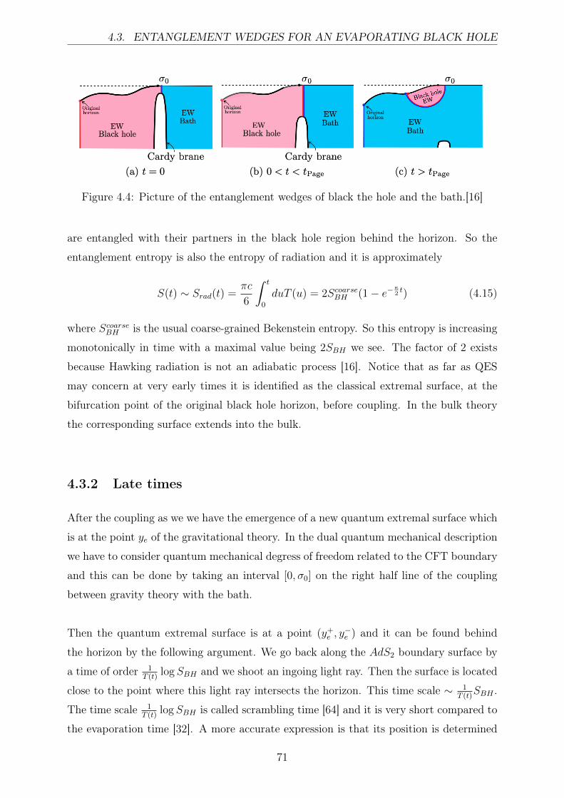
4.3. ENTANGLEMENT WEDGES FOR AN EVAPORATING BLACK HOLE
Figure 4.4: Picture of the entanglement wedges of black the hole and the bath.[16]
are entangled with their partners in the black hole region behind the horizon. So the
entanglement entropy is also the entropy of radiation and it is approximately
S(t) ∼ Srad(t) =πc
6
∫ t
0
duT (u) = 2ScoarseBH (1− e−κ2t) (4.15)
where ScoarseBH is the usual coarse-grained Bekenstein entropy. So this entropy is increasing
monotonically in time with a maximal value being 2SBH we see. The factor of 2 exists
because Hawking radiation is not an adiabatic process [16]. Notice that as far as QES
may concern at very early times it is identified as the classical extremal surface, at the
bifurcation point of the original black hole horizon, before coupling. In the bulk theory
the corresponding surface extends into the bulk.
4.3.2 Late times
After the coupling as we we have the emergence of a new quantum extremal surface which
is at the point ye of the gravitational theory. In the dual quantum mechanical description
we have to consider quantum mechanical degress of freedom related to the CFT boundary
and this can be done by taking an interval [0, σ0] on the right half line of the coupling
between gravity theory with the bath.
Then the quantum extremal surface is at a point (y+e , y
−e ) and it can be found behind
the horizon by the following argument. We go back along the AdS2 boundary surface by
a time of order 1T (t)
logSBH and we shoot an ingoing light ray. Then the surface is located
close to the point where this light ray intersects the horizon. This time scale ∼ 1T (t)
SBH .
The time scale 1T (t)
logSBH is called scrambling time [64] and it is very short compared to
the evaporation time [32]. A more accurate expression is that its position is determined
71

4.3. ENTANGLEMENT WEDGES FOR AN EVAPORATING BLACK HOLE
Figure 4.5: The entanglement wedge of the black hole at times which in 2d is a sspatialslice. In 3d gravity picture there is also a RT/HRT surface [16]
Figure 4.6: The entanglement wedge of the radiation including a contribution from theinitial black hole horizon, and a contribution from the IR cutoff in the CFT. [16]
by
y+e = t− 1
2πT (t)log
SBH(T (t))− S0
c+ ... (4.16)
with S0 << ScoarseBH be the extremal entropy associated with the black hole before the
coupling with the bath. Therefore the entanglement entropy reduces to an RT/HRT
surface from the point ye to σ0 which is an interval contribution and the entanglement
wedge of the black hole is the causal domain of this interval. The entanglement entropy
of the black hole then for this extremal surface is given by
S(t) = ScoarseBH (T (t)) +O(log) (4.17)
so the dominant term is the coarse-grained Bekenstein term and also there are some loga-
rithmic contributions of initial state entropy. The main point of this expression is that it
decreases monotonically since the temperature decreases. Now at last let’s discuss about
radiation which is the most important point in order to derive the form of Page curve.
As we saw at early times the contribution from the early time QES gives an increasing
72

4.3. ENTANGLEMENT WEDGES FOR AN EVAPORATING BLACK HOLE
entropy of radiation which is approximately equal to the entropy of the black hole. As
we mentioned above the entanglement of radiation and the black hole can be viewed as
the study of the entanglement of black hole and the CFT bath and so we have to study
the entropy of the CFT in the bath, on an interval outside σ0, [σ0, σIR] ≡ ΣR where
σIR > tevap is a cut-off point large enough so that we assume all entropy from radiation
emitted from the black hole is approximately contained entirely there. The entanglement
wedge in 2-dimensional point of view should be this interval which would reproduce an
increasing entropy of radiation and give Hawking result. However at late times the en-
tanglement wedge of the black hole does not contain the whole interior. Thus we assume
now that the rest of the interior belongs to the wedge of radiation.
The result is a that apart from the main region of radiation there is also a manifestly
disconnected region behind the horizon which is called the "island" which is seperated
from the "mainland" which is the interval [σ0, σIR]. This seems rather odd, however, when
we take the dual picture we see directly that the two regions are actually connected via
the extra dimension in the bulk theory. Therefore, considering that at late times the en-
tanglement wedge of radiation is identified by the entanglement wedge of the bath indeed
it contains three extremal surfaces. One concerns the initial extremal surface of the of
the original black hole horizon, which is located at the leftmost point of the island. The
second is an extremal surface found from RT/HRT prescription from σ0 to the Planck
brane. This extremal surface coincides with the surface discussed for black hole and it
is the minimal at late times. Finally there is another extremal surface which starts at
σIR and finishes at Cardy brane which at late times is immersed very deep into the bulk
giving a very small entropy
S ∼ c
6log σIR << ScoarseBH
. The essential point of this island prescription is that we can have in 2-dimensional
consideration, at late times, a disconnected entanglement wedge for radiation which is
actually connected via the extra dimension of the dual theory in 3 dimensions. Therfore,
the equation (4.2) can be generalized in order to include the island configuration of the
entanglement wedge and then the entanglement entropy of radiation is
Srad = minextr
(Area(X )
4G(3)N
+ Seff (ΣR ∪ Σisland))
(4.18)
73

4.3. ENTANGLEMENT WEDGES FOR AN EVAPORATING BLACK HOLE
Figure 4.7: Page curve of Hawking radiation of JT gravity model coupling to zero tem-perature CFT bath.[16]
where Seff is the effective entropy of radiation in semiclassical geometry approximation
taking into account the island configuration of the entanglement wedge.
4.3.3 Reproducing the Page curve
So now practically our task is accomplished. The time evolution of the entropy of Hawking
radiation will be configured by the above extremal surfaces. Initially the radiation will rise
following the equation (4.14), then at Page time its value is equal to Bekenstein entropy
which subsequently coincides with the entanglement entropy of the Black hole and at
this point, with a minimal extremal surface concerning the original black hole. After this
point there is a phase transition in entanglement wedge and minimal extremal surface
which gives rise to radiation entropy at late times is the one concerning the black hole at
late times and the entropy gradually decreases. Thus we have reproduced the Page curve!
Of course details about how smooth is the phase transition or when exactly is have to
do with quantum effects (see [15]) but the main point of this model is that it describes a
black hole system which illustrates an evaporating black hole and respect unitarity.
74

Conclusion
So the conclusion of the entire discussion in this thesis is that indeed the Page curve
can be derived holographically, by considering a black hole in a 2d gravity theory with
holographic matter coupled to a 2d CFT bath. So in terms of AdS/CFT correspondence
black holes as quantum systems evolve in unitary fashion. This prescription gives rise to
an entanglement wedge which contains a disconnected island region in the interior, in 2-
dimensions and it is connected with the exterior mainland region via the third dimension
of the holographic dual theory.
The derivation of the Page curve with this holographic prescription is surely a positive
step towards finding a consistent solution to information paradox. However, again here
we have to emphasize that all this discussion has not given any new detail about the final
state and thus about the corresponding density matrix. We actually have discovered a
delicate way by using RT/HRT formula in order to calculate entanglement entropies but
we do not know precisely the final states which are determined potentially by gravity ef-
fects during the final stages and therefore, we do not have a precise result of the elements
of density matrix respectively.
This field is still very new and there is surely lot of work to be done. More specifi-
cally in 2020 new studies have been published which analyze the same problem but the
CFT bath is now a thermal bath of finite temperature [65] and also the case of the 2-
dimensional gravity+matter theory in an asympotically flat spacetime instead of asymp-
totically AdS2[66]. The whole discussion we have done was about 2-dimensional theory
but it can be generalized to d-dimensions, even though, as we had mentioned the coupling
of gravity and holographic matter becomes far more complicated.
75

Bibliography
[1] James M. Bardeen, B. Carter, and S.W. Hawking. The Four laws of black holemechanics. Commun. Math. Phys., 31:161–170, 1973.
[2] Jacob D. Bekenstein. Generalized second law of thermodynamics in black holephysics. Phys. Rev. D, 9:3292–3300, 1974.
[3] S.W. Hawking. Particle Creation by Black Holes. In 1st Oxford Conference onQuantum Gravity, pages 219–267, 8 1975.
[4] S.W. Hawking. Breakdown of Predictability in Gravitational Collapse. Phys. Rev.D, 14:2460–2473, 1976.
[5] Gerard ’t Hooft. Dimensional reduction in quantum gravity. Conf. Proc. C,930308:284–296, 1993.
[6] Leonard Susskind. The World as a hologram. J. Math. Phys., 36:6377–6396, 1995.
[7] Don N. Page. Average entropy of a subsystem. Phys. Rev. Lett., 71:1291–1294, 1993.
[8] Don N. Page. Information in black hole radiation. Phys. Rev. Lett., 71:3743–3746,1993.
[9] Don N. Page. Time Dependence of Hawking Radiation Entropy. JCAP, 09:028, 2013.
[10] Shinsei Ryu and Tadashi Takayanagi. Holographic derivation of entanglement en-tropy from AdS/CFT. Phys. Rev. Lett., 96:181602, 2006.
[11] Veronika E. Hubeny, Mukund Rangamani, and Tadashi Takayanagi. A Covariantholographic entanglement entropy proposal. JHEP, 07:062, 2007.
[12] Juan Maldacena. Black hole entropy and quantum mechanics. 10 2018.
[13] Netta Engelhardt and Aron C. Wall. Quantum Extremal Surfaces: HolographicEntanglement Entropy beyond the Classical Regime. JHEP, 01:073, 2015.
[14] Ahmed Almheiri, Netta Engelhardt, Donald Marolf, and Henry Maxfield. The en-tropy of bulk quantum fields and the entanglement wedge of an evaporating blackhole. JHEP, 12:063, 2019.
[15] Geoffrey Penington. Entanglement Wedge Reconstruction and the Information Para-dox. JHEP, 09:002, 2020.
[16] Ahmed Almheiri, Raghu Mahajan, Juan Maldacena, and Ying Zhao. The Page curveof Hawking radiation from semiclassical geometry. JHEP, 03:149, 2020.
76

BIBLIOGRAPHY
[17] Fay Dowker . In Black Holes Lecture notes MSc QFFF Imperial College London.
[18] Jerome Gauntlett . In Black Holes Lecture notes MSc QFFF Imperial College Lon-don.
[19] Harvey Reall . In Part 3 Black Holes Lecture notes, University of Cambridge, pages111–147, 2016.
[20] P.K. Townsend. Black holes: Lecture notes. 7 1997.
[21] Roy P. Kerr. Gravitational collapse and rotation. 1965.
[22] W. Israel. Gravitational Collapse and Causality. Phys. Rev., 153:1388–1393, 1967.
[23] B. Carter. Axisymmetric Black Hole Has Only Two Degrees of Freedom. Phys. Rev.Lett., 26:331–333, 1971.
[24] S.W. Hawking and G.F.R. Ellis. The Large Scale Structure of Space-Time. CambridgeMonographs on Mathematical Physics. Cambridge University Press, 2 2011.
[25] D.C. Robinson. Uniqueness of the Kerr black hole. Phys. Rev. Lett., 34:905–906,1975.
[26] J.B. Hartle and S.W. Hawking. Solutions of the Einstein-Maxwell equations withmany black holes. Commun. Math. Phys., 26:87–101, 1972.
[27] Yu-Lei Feng and Yi-Xin Chen. Nonthermal Spectrum of Hawking Radiation. 112015.
[28] Andrew Tolley. Lecture notes in Foundations of Quantum Mechanics, Imperial Col-lege London. 2020.
[29] Daniel Harlow. Jerusalem Lectures on Black Holes and Quantum Information. Rev.Mod. Phys., 88:015002, 2016.
[30] F. Benatti, R. Floreanini, F. Franchini, and U. Marzolino. Entanglement in indistin-guishable particle systems. Phys. Rept., 878:1–27, 2020.
[31] Wojciech Hubert Zurek. Decoherence, einselection, and the quantum origins of theclassical. Rev. Mod. Phys., 75:715–775, 2003.
[32] Ahmed Almheiri, Thomas Hartman, Juan Maldacena, Edgar Shaghoulian, andAmirhossein Tajdini. The entropy of Hawking radiation. 6 2020.
[33] Tatsuma Nishioka, Shinsei Ryu, and Tadashi Takayanagi. Holographic EntanglementEntropy: An Overview. J. Phys. A, 42:504008, 2009.
[34] R. B. Mann. Black Holes: Thermodynamics, Information, and Firewalls. pages61–63, 2015.
[35] Andrew Strominger and Cumrun Vafa. Microscopic origin of the Bekenstein-Hawkingentropy. Phys. Lett. B, 379:99–104, 1996.
[36] Samir D. Mathur. What Exactly is the Information Paradox? Lect. Notes Phys.,769:3–48, 2009.
77

BIBLIOGRAPHY
[37] Samir D. Mathur. The Information paradox: A Pedagogical introduction. Class.Quant. Grav., 26:224001, 2009.
[38] Samir D. Mathur. The information paradox: conflicts and resolutions. Pramana,79:1059–1073, 2012.
[39] J.B. Hartle and S.W. Hawking. Path Integral Derivation of Black Hole Radiance.Phys. Rev. D, 13:2188–2203, 1976.
[40] John Preskill. Do black holes destroy information? In International Symposium onBlack holes, Membranes, Wormholes and Superstrings, pages 22–39, 1 1992.
[41] Robert M. Wald. Black hole entropy is the Noether charge. Phys. Rev. D, 48(8):3427–3431, 1993.
[42] Aron C. Wall. A proof of the generalized second law for rapidly changing fields andarbitrary horizon slices. Phys. Rev. D, 85:104049, 2012. [Erratum: Phys.Rev.D 87,069904 (2013)].
[43] Tom Banks, W. Fischler, S.H. Shenker, and Leonard Susskind. M theory as a matrixmodel: A Conjecture. Phys. Rev. D, 55:5112–5128, 1997.
[44] Ted Jacobson. Boundary unitarity and the black hole information paradox. Int. J.Mod. Phys. D, 22:1342002, 2013.
[45] S.W. Hawking. Black hole explosions. Nature, 248:30–31, 1974.
[46] Juan Martin Maldacena. The Large N limit of superconformal field theories andsupergravity. Int. J. Theor. Phys., 38:1113–1133, 1999.
[47] Juan Maldacena. The Gauge/gravity duality, pages 325–347. 2012.
[48] Toby Wiseman. Notes on AdS/CFT correspondence, QFFF Special Topics ImperialCollege London, 2020 .
[49] Ofer Aharony, Steven S. Gubser, Juan Martin Maldacena, Hirosi Ooguri, and YaronOz. Large N field theories, string theory and gravity. Phys. Rept., 323:183–386, 2000.
[50] Veronika E. Hubeny. The AdS/CFT Correspondence. Class. Quant. Grav.,32(12):124010, 2015.
[51] Niklas Beisert et al. Review of AdS/CFT Integrability: An Overview. Lett. Math.Phys., 99:3–32, 2012.
[52] Erdmenger J. (2015). Gauge/Gravity Duality: Foundations Ammon, M. and Appli-cations. Cambridge: Cambridge University Press. doi:10.1017/CBO9780511846373.
[53] Joao Penedones. TASI lectures on AdS/CFT. In Theoretical Advanced Study Institutein Elementary Particle Physics: New Frontiers in Fields and Strings, pages 75–136,2017.
[54] Carlos Alfonso Bayona and Nelson R.F. Braga. Anti-de Sitter boundary in Poincarecoordinates. Gen. Rel. Grav., 39:1367–1379, 2007.
78

BIBLIOGRAPHY
[55] Masaya Fukami Introduction to the Ryu-Takayanagi Formula PHYS 48300 StringTheory-1. 2018.
[56] Jeongseog Lee, Lauren McGough, and Benjamin R. Safdi. Rényi entropy and geom-etry. Phys. Rev. D, 89(12):125016, 2014.
[57] Shinsei Ryu and Tadashi Takayanagi. Aspects of Holographic Entanglement Entropy.JHEP, 08:045, 2006.
[58] Maximo Banados, Claudio Teitelboim, and Jorge Zanelli. The Black hole in three-dimensional space-time. Phys. Rev. Lett., 69:1849–1851, 1992.
[59] Thomas Faulkner, Aitor Lewkowycz, and Juan Maldacena. Quantum corrections toholographic entanglement entropy. JHEP, 11:074, 2013.
[60] R. Jackiw. Lower Dimensional Gravity. Nucl. Phys. B, 252:343–356, 1985.
[61] C. Teitelboim. Gravitation and Hamiltonian Structure in Two Space-Time Dimen-sions. Phys. Lett. B, 126:41–45, 1983.
[62] Lisa Randall and Raman Sundrum. An Alternative to compactification. Phys. Rev.Lett., 83:4690–4693, 1999.
[63] Steven S. Gubser. AdS / CFT and gravity. Phys. Rev. D, 63:084017, 2001.
[64] Patrick Hayden and John Preskill. Black holes as mirrors: Quantum information inrandom subsystems. JHEP, 09:120, 2007.
[65] Hong Zhe Chen, Zachary Fisher, Juan Hernandez, Robert C. Myers, and Shan-MingRuan. Evaporating Black Holes Coupled to a Thermal Bath. 7 2020.
[66] Friðrik Freyr Gautason, Lukas Schneiderbauer, Watse Sybesma, and Lárus Thor-lacius. Page Curve for an Evaporating Black Hole. JHEP, 05:091, 2020.
79