information and price dispersion: evidence from retail

Information and Price Dispersion:

Evidence from Retail Gasoline

⇤

Dieter Pennerstorfer† Philipp Schmidt-Dengler‡ Nicolas Schutz§

Christoph Weiss¶ Biliana Yontcheva¶

February 21, 2014

Abstract

We examine the relationship between information and price dispersion in the retail

gasoline market. We first show that the clearinghouse models in the spirit of Stahl

(1989) generate an inverted-U relationship between information and price dispersion.

Past empirical studies of this relationship have relied on (intertemporal) variation in

internet usage and adoption to measure the number of consumers that have access to

the clearinghouse. We construct a new measure of information based commuter data

from Austria. Regular commuters can freely sample gasoline prices on their commuting

route, giving us spatial variation in the share of informed consumers. We use detailed

information on gas station level price to construct various measures of price dispersion.

Our empirical estimates of the relationship are in line with the theoretical predictions.

Keywords: Search, Price Dispersion, Retail Gasoline, Commuter Data

JEL Classification: D43, D83, L13

⇤We thank seminar participants at DIW Berlin, St. Gallen, the University of Queensland, Queensland Uni-versity of Technology, Vienna University of Economics and Business, WIFO, and the 2014 Winter Marketing-Economics Summit for helpful comments. Schmidt-Dengler is also a�liated with CEPR, CES-Ifo, and ZEW.

†Austrian Institute of Economic Research‡University of Mannheim, also a�liated with CEPR, CES-Ifo, and ZEW.§University of Mannheim¶Vienna University of Economics and Business

1

1 Introduction

Price competition in homogeneous goods markets rarely yields results in market outcomes

in line “law of one price.” To the contrary, price dispersion is ubiquitous and di↵erences in

location, cost or services attributed to seemingly homogeneous goods cannot fully explain

observed price dispersion. In his seminal paper on “The Economics of Information,” Stigler

(1961) o↵ered the first search-theoretic rationale for price dispersion. In fact, Stigler claims

that “price dispersion is a manifestation - and, indeed, it is the measure - of ignorance in the

market” (p.214). Following Stigler’s seminal work, it has been shown that price dispersion

can arise as an equilibrium phenomenon in a homogeneous goods market with symmetric

firms when consumers are not fully informed about prices (see Baye et al. (2006)).

The present paper examines the relationship between information and price dispersion.

We first derive the global relationship between information and price dispersion in a “clear-

inghouse model” as introduced by Varian (1980) and further developed by Stahl (1989).

Consumers are aware of sellers’ (randomized) pricing strategy, but di↵er in the degree of

information. For some, obtaining an additional price quote is costly. Others are aware of

all prices charged in the relevant market: they have access to the “clearinghouse.” At the

very extremes, this model predicts no price dispersion. If no consumer has access to the

clearinghouse, all firms will charge the monopoly price. Conversely, if all consumers are fully

informed, this corresponds to Bertrand competition, and price equals marginal cost. While

the existing literature has observed that price dispersion is not a monotone function of the

fraction of informed consumers (see Conclusion 3 in Baye et al. (2006)), we prove that the

model generates an inverse-U relationship globally.

We then test this prediction. Price dispersion has been observed and analyzed in a large

number of markets (Baye et al. (2006)). These studies examine a variety of issues, including

the di↵erence between online and o✏ine price dispersion, the e↵ect of the number of sell-

ers, the relationship between dispersion and purchase frequency, and the dynamics of online

price dispersion. Empirical studies focusing on the impact of consumer information on price

dispersion, however, are rare; the challenge here is to find a good measure for the fraction of

informed consumers. Sorensen (2000) finds empirical evidence that purchase frequency (of

drugs) is negatively correlated with both price-cost margins and dispersion, which is inter-

preted evidence in support of search models. Analyzing price dispersion in the market for

life insurances, Brown and Goolsbee (2002) use variation in the share of consumers searching

on the Internet over a six year period as their measure of consumer information. They find

that the early increase in internet usage has resulted in an increase in price dispersion at

2

very low levels and in decrease later on. Tang et al. (2010) examine the impact of changes in

shopbot use over time on pricing behavior in the Internet book market. They observe that

an increase in shopbot use is correlated with a decrease in price dispersion over time.

While analysis of price dispersion in online markets versus o✏ine markets has provided useful

insights, we argue that it may be preferable to look at the relationship between information

and price dispersion in an o✏ine market. First, Ellison and Ellison (2005) and Ellison and

Ellison (2009) question the extent to which the Internet has actually reduced consumer search

costs. They argue - and also provide evidence for their claim - that firms in online markets

often engage in “bait and switch” as well as “obfuscation” strategies that frustrate consumer

search and make search more costly 1. Second, even when focusing on a homogeneous prod-

uct sold online (which is a questionable assumption in the case of insurance, for example),

it remains unclear whether buying and selling over the Internet eliminates all relevant seller

characteristics. Baye and Morgan (2001) stress that consumers’ and firms’ decisions to use

Internet shopbots are endogenous. Consumers’ expected gains from obtaining information

form shopbots will increase with the dispersion of prices in the market which implies that a

correlation between the share of internet users and price dispersion cannot be given a causal

interpretation.

Our paper follows a di↵erent approach. We adopt an alternative interpretation of the “clear-

inghouse” by employing spatial variation in commuting behavior. Commuters are able to

freely sample all price quotes for gasoline along their commute. Using detailed data on com-

muting behavior from the Austrian census, we construct the share of commuters passing by

an individual gas station. We use this as our measure of the fraction of informed consumers.

We combine this with data on retail gasoline prices at the station level to test the relationship

between consumer information and price dispersion. To the best of our knowledge, this is

the first attempt to create a measure of informed consumers not related to internet usage or

access. We believe that our setting is closer in spirit to the seminal clearinghouse models of

Varian (1980) and Stahl (1989) for the following reasons: (a) firms’ abilities to obfuscate con-

sumers search and learning e↵orts are limited in this market, (b) gasoline is a homogeneous

product and seller characteristics can be adequately controlled, (c) we observe substantial

variation in our measure of the share of informed consumers enabling us to test the global

1According to Ellison and Ellison (2005) “the Internet makes it easy for e-retailers to o↵er complicatedmenus of prices (for example, with di↵erent options for shipping), to make price o↵ers that search engineswill misinterpret (like products bundled together), to personalize prices and to make the process of examiningan o↵er su�ciently time consuming so that customers will not want to do it many times” (p. 153). Theyconclude that “whether the Internet will prove to aid search or obfuscation more is not clear a priori” (p.153) and that “Knowledgeable economists would also not have put much faith in how the Internet wouldlead literally to the ’Law of One Price”’ (p. 149)

3

prediction derived from theory, and (d) the consumers’ decisions to commute - and thus to

become better informed - is not determined by regional di↵erences in price dispersion which

allows a causal interpretation of our empirical results.

Our empirical findings are surprisingly robust. For all commonly used measures of price

dispersion, we cannot reject the null-hypothesis of an inverted-U relationship. This result is

also robust to di↵erent market definitions. As a further robustness check we also test a key

implication of the model: Price levels decline with the fraction of informed consumers.

The remainder of the paper is organized as follows. Section 2 presents the clearinghouse

model and derives the testable prediction regarding the relationship between information and

price dispersion. Section 3 describes the industry, the retail price data, and our construction

of a measure of informed consumers from the information on commuting behavior in the

Census. Section 4 presents the empirical results. Section 5 concludes.

2 Information and Price Dispersion in Clearinghouse

Models

In this section, we present Stahl (1989)’s search model with unit demand, which encompasses

Varian (1980)’s model of sales as a special case. There is a finite number of firms N > 1

selling a homogeneous product. They face constant marginal cost c and compete in prices.

There is a unit mass of consumers with unit demand for the product and maximal willingness

to pay v > c. A share µ 2 (0, 1) of consumers are “informed” consumers who observe all

prices through the clearinghouse. We sometimes refer to these consumers as “shoppers,”

because they sample all prices. These consumers buy at the lowest price provided that it

does not exceed their willingness to pay v. The remaining fraction of consumers (1 � µ) is

referred to as “non-shoppers”. They engage in sequential search with costless recall: the first

sample is free, thereafter each sample costs s > 0.

Equilibrium price distribution. It is well known that for any µ 2 (0, 1) there is no pure

strategy equilibrium, but that there exists a unique symmetric mixed strategy equilibrium.

The equilibrium price distribution is given by

F (p) = 1�

✓1� µ

µ

1

N

p� p

p� c

◆ 1N�1

(1)

for all p in support⇥p, p⇤. Solving for F (p) = 0, we obtain the lower bound of support:

p = c + p�c

1+ µ1�µN

. The upper bound of the support is pinned down by the non-shoppers’

4

optimal search behavior. Let (r) be the expected net benefit of searching when facing a

price of r:

(r) = v � s�

Zr

p

pdF (p)� (1� F (r))r � (v � r) =

Zr

p

(r � p)dF (p)� s.

Then the upper bound of the support is such that (p) 0, because otherwise p would lead

to zero profit. It must also hold that (p) � 0 if p < v, because otherwise strictly increase

its profit by charging a price of p+ ". Since is strictly increasing in p, there exists a unique

p which satisfies these conditions. Janssen et al. (2011) show that (r) = 0 if and only if

r = ⇢ ⌘ c+ s

1�↵

, where ↵ =R 1

01

1+ µ1�µNz

N�1dz 2 (0, 1). It follows that the upper bound of the

support is given by p = min(⇢, v).

Observe that if s � v � c, then non-shopper never find it profitable to search and our

model is equivalent to Varian’s model of sales. In this case, ⇢ > v and p = v for all (µ,N),

as in Varian (1980). Conversely, if s < v � c, then there exists a unique µ 2 (0, 1) such that

p = v if µ µ and p = ⇢ if µ � µ.2 We thus have fully characterized the equilibrium price

distribution in terms of the parameters (c, v, s, µ,N). Expected Price. The expected price is

given by

E(p) =

Zmin(⇢,v)

p

pdF (p),

= (1 + ↵) ⇤ (min(⇢, v)� c).

It is immediate, that the expected price is decreasing in the fraction of shoppers µ, as both ↵

and ⇢ are decreasing in µ. In order to validate the model, we will test the following prediction

due toStahl (1989):

Remark 1. The expected price E(p) is declining in the proportion of informed consumers µ.

The intuition behind this result is very simple. As the proportion of shoppers increases,

firms are increasingly tempted to attract shoppers by charging the lowest price. As a con-

sequence, both the upper bound and the lower bound of the distribution shift down, and

probability mass shifts down everywhere.

Price dispersion. Various measures of price dispersion have been used in the literature.

We will focus on one common measure of price dispersion: the Value of Information (VOI).

It corresponds to a consumer’s expected benefit of being informed: the di↵erence between

2This follows from the fact that ⇢ is strictly decreasing in µ and has limits +1 and c + s in 0 and 1,respectively.

5

the expected price and the expected minimum price in the market:

E(p� pmin

) =

Zp

p

ph1�N [1� F (p)]N�1

idF (p), (2)

where pmin

= min{p1, p2, . . . , pN}. Substituting the equilibrium price distribution (1) into

equation (2) and applying change of variables z = 1� F (p) yields

E(p� pmin

) =

Z 1

0

c+

p� c

1 + µ

1�µ

NzN�1

!�1�NzN�1

�dz,

= (p� c)

✓↵�

1� µ

µ(1� ↵)

◆.

When µ is close enough to zero, p = v and the value of information goes to zero as µ goes

to zero. Conversely, when µ is in the neighborhood of 1, p is equal to either c + s

1�↵

or v.

In both cases, the value of information goes to zero as µ goes to 1. We prove the following

proposition:

Proposition 1. There is an inverse-U shaped relationship between price dispersion E(p �

pmin

) and the proportion of informed consumers µ: there exists a value µ 2 (0, 1) such that

price dispersion is increasing in µ on (0, µ) and decreasing in µ on (µ, 1).

Proof. It follows from Lemma 1 in Tappata (2009) that ↵�

1�µ

µ

(1�↵) is strictly concave in

µ. Combining this with the fact that E(p� pmin

) goes to 0 as µ goes to 0 and 1 proves the

proposition for the case s � v � c.

Next, assume s < v � c. Then E(p � pmin

) is strictly concave on interval (0, µ], and we

now claim that it is strictly decreasing on [µ, 1). If µ � µ, then v = ⇢ and E(p � pmin

)

simplifies to s⇣

↵

1�↵

�

1�µ

µ

⌘, which is strictly decreasing in µ by Lemma 1, stated and proven

in Appendix A.. This concludes the proof.

To obtain intuition behind this result, consider starting at the µ = 0, where all firms

charge the monopoly price v and there is zero price dispersion. As µ increases, firms have

an incentive to charge lower prices to capture the shoppers. Hence the lower bound of the

distribution shifts and dispersion increases. As µ increases further, more mass shifts towards

the lower bound, so that eventually, price dispersion falls. In the case µ � µ, the reserve price

⇢ is binding, and therefore, both the upper bound and the lower bound of the distribution

are shifted down. Lemma 1 shows that this possible widening of the support never o↵sets

the shift in mass towards towards the lower bound.

6

3 Industry Background and Data

3.1 Gasoline Prices and Stations

Our empirical analysis focuses on the retail gasoline market in Austria. The retail gasoline

market is particularly suitable for our purpose: Retail gasoline is a fairly homogeneous prod-

uct with the main source of di↵erentiation being spatial location, which is easily controlled

for. Further, consumers primarily visit gas stations to purchase gasoline, so that our analysis

is less likely to be confounded by consumers purchasing multiple products (see Hosken et al.

(2008)).

We use quarterly data on diesel prices at the gas station level3 from October 1999 to March

2005. Prices from each station were collected within three days at each time period by the

Austrian Chamber of Labor (“Arbeiterkammer”). We merge the price data with information

on the geographical location of all 2,814 gas stations as well as their characteristics: the

number of pumps, whether the station has service bays, a convenience store etc..4 Retail

prices are nominal and measured in Euro cents per liter, including fuel tax (a per unit tax)

and value added tax. In total, these taxes amount to about 55% of the total diesel price.

Unfortunately, the Austrian Chamber of Labor did not obtain prices for all active gasoline

stations in every quarter. As there is no systematic pattern with respect to whether a

particular station was sampled in a given year, we are not concerned with selection issues.

We will however control for unsampled competitors in a given market in the price-dispersion

regressions.

To characterize the spatial distribution of suppliers and to measure distances between

gasoline stations we collect information about the structure of the road network. Using data

from ArcData Austria and the ArcGIS extension WIGeoNetwork, the geographical location

of the individual gasoline stations is linked to information on the Austrian road system.5

This allows us to generate accurate measures of distance as well as the commuting be-

haviour across the road network.3Unlike in North America, diesel-engined vehicles are most popular, accounting for more than 50% of

registered passenger vehicles in Austria in 2005 (Statistik Austria, 2006).4The information on gas station characteristics have been collected by the company Experian Catalist in

August 2003, see http://www.catalist.com for company details.5We further supplement the individual data with demographic data (population density, ...) of the munic-

ipality, where the gasoline station is located. This information is collected by the Austrian statistical o�ce(Statistik Austria).

7

3.2 Commuters as Informed Consumers

The main idea behind our measure of information is that commuters can freely sample

prices along their daily commuting path.6 We therefore rely on the fraction of long-distance

commuters as a measure of the ”shoppers” on the market. We implement this idea by sorting

the potential consumers of a given station into two groups based on the length and regularity

of their commute. We define individuals who travel by car as a driver on a daily basis to

work and go beyond the border of their own municipality as long-distance commuters. Our

estimate of the share of informed consumers faced by a gas station depends on the relative

size of this group compared to the total size of the station’s market.

Commuter flows

According to the 2001 census, 2,051,000 people in Austria go to work by car on a daily

basis. For 1,396,426 of these people, the commute involves regular travel beyond the bound-

aries of their home municipality. We will refer to these consumers as informed consumers.

The Austrian Statistical O�ce provides detailed information on the number of individuals

commuting from a given ”origin-municipality” o to a di↵erent ”destination-municipality”

d for each of the 2381 administrative units in Austria. All commuters are assigned to an

origin-destination pair of municipalities based on their home address and their workplace

address.7 Since municipalities are generally very small regional units, this allows us to create

an intricate description of the commuting patterns in Austria. The average (median) mu-

nicipality is 13.8 (9.4) square-miles large, has 3373 (1575) inhabitants and 1.19 (1) gasoline

stations. For the average (median) municipality strictly positive commuter flows to 51 (32)

other municipalities are observed.

In order to assign commuter flows to gas stations we merge the municipality-level data on

the spatial distribution of commuters with data on the precise location of each station within

the road network using GIS software (WiGeoNetwork Analyst, ArcGIS). This allows us to

determine how many individuals reside in the municipality where a given station i is located

but commute to a di↵erent municipality. Let this number be denoted by Cout

i

, the number

of individuals commuting out of the municipality where station i is located. Commuters

who work in the municipality of station i but live in a di↵erent municipality also belong to

6Houde (2012) emphasizes the role of commuters on firms’ pricing decisions. Commuters also tend to pur-chase more fuel, than their non-commuting counterparts and therefore gain more from information regardingthe price distribution (Marvel (1976), Sorensen (2000)).

7The data were prepared by the Austrian Federal Ministry for Transport, Innovation and Technology forthe project ‘Verkehrsprognose Osterreich 2025+’. We are thankful to the ministry for sharing the data withus.

8

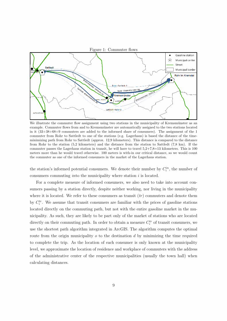
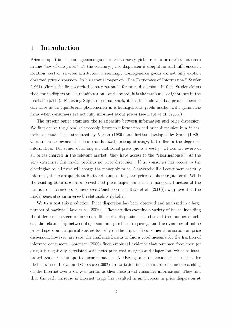
Figure 1: Commuter flows

We illustrate the commuter flow assignment using two stations in the municipality of Kremsmunster as anexample. Commuter flows from and to Kremsmunster are automatically assigned to the two stations locatedin it (33+38+68+9 commuters are added to the informed share of consumers). The assignment of the 1commuter from Rohr to Sattledt to one of the stations (e.g. Lagerhaus) is based the distance of the time-minimizing path from Rohr to Sattledt (approx. 12,9 kilometers). This distance is compared to the distancefrom Rohr to the station (5,2 kilometers) and the distance from the station to Sattledt (7,8 km). If thecommuter passes the Lagerhaus station in transit, he will have to travel 5,2+7,8=13 kilometers. This is 100meters more than he would travel otherwise. 100 meters is with-in our critical distance, so we would countthe commuter as one of the informed consumers in the market of the Lagerhaus station.

the station’s informed potential consumers. We denote their number by C in

i

, the number of

consumers commuting into the municipality where station i is located.

For a complete measure of informed consumers, we also need to take into account con-

sumers passing by a station directly, despite neither working, nor living in the municipality

where it is located. We refer to these consumers as transit (tr) commuters and denote them

by Ctr

i

. We assume that transit consumers are familiar with the prices of gasoline stations

located directly on the commuting path, but not with the entire gasoline market in the mu-

nicipality. As such, they are likely to be part only of the market of stations who are located

directly on their commuting path. In order to obtain a measure Ctr

i

of transit consumers, we

use the shortest path algorithm integrated in ArcGIS. The algorithm computes the optimal

route from the origin municipality o to the destination d by minimizing the time required

to complete the trip. As the location of each consumer is only known at the municipality

level, we approximate the location of residence and workplace of commuters with the address

of the administrative center of the respective municipalities (usually the town hall) when

calculating distances.

9

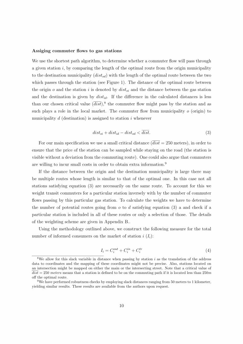
Assiging commuter flows to gas stations

We use the shortest path algorithm, to determine whether a commuter flow will pass through

a given station i, by comparing the length of the optimal route from the origin municipality

to the destination municipality (distod

) with the length of the optimal route between the two

which passes through the station (see Figure 1). The distance of the optimal route between

the origin o and the station i is denoted by distoi

and the distance between the gas station

and the destination is given by distid

. If the di↵erence in the calculated distances is less

than our chosen critical value (dist),8 the commuter flow might pass by the station and as

such plays a role in the local market. The commuter flow from municipality o (origin) to

municipality d (destination) is assigned to station i whenever

distoi

+ distid

� distod

< dist. (3)

For our main specification we use a small critical distance (dist = 250 meters), in order to

ensure that the price of the station can be sampled while staying on the road (the station is

visible without a deviation from the commuting route). One could also argue that commuters

are willing to incur small costs in order to obtain extra information.9

If the distance between the origin and the destination municipality is large there may

be multiple routes whose length is similar to that of the optimal one. In this case not all

stations satisfying equation (3) are necessarily on the same route. To account for this we

weight transit commuters for a particular station inversely with by the number of commuter

flows passing by this particular gas station. To calculate the weights we have to determine

the number of potential routes going from o to d satisfying equation (3) a and check if a

particular station is included in all of these routes or only a selection of those. The details

of the weighting scheme are given in Appendix B..

Using the methodology outlined above, we construct the following measure for the total

number of informed consumers on the market of station i (Ii

):

Ii

= Cout

i

+ C in

i

+ Ctr

i

(4)

8We allow for this slack variable in distance when passing by station i as the translation of the addressdata to coordinates and the mapping of these coordinates might not be precise. Also, stations located onan intersection might be mapped on either the main or the intersecting street. Note that a critical value ofdist = 250 meters means that a station is defined to be on the commuting path if it is located less than 250mo↵ the optimal route.

9We have performed robustness checks by employing slack distances ranging from 50 meters to 1 kilometer,yielding similar results. These results are available from the authors upon request.

10

We approximate the number of uninformed consumers on the market (Ui

) with the number

of employed individuals living in the municipality in which the station is located who do not

regularly commute over long distances by car.10

Having determined the number of uninformed consumers, we calculate a station-specific

proxy for the fraction of informed consumers in station i’s market µi

:

µi

=Ii

Ui

+ Ii

(5)

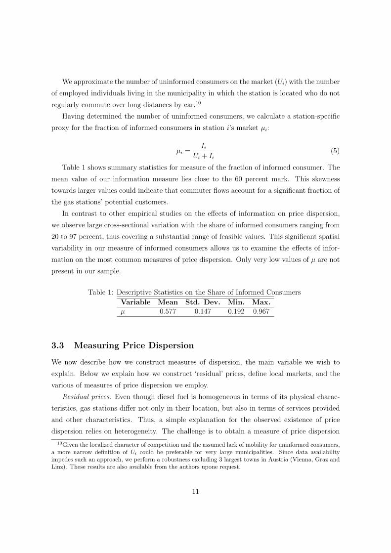
Table 1 shows summary statistics for measure of the fraction of informed consumer. The

mean value of our information measure lies close to the 60 percent mark. This skewness

towards larger values could indicate that commuter flows account for a significant fraction of

the gas stations’ potential customers.

In contrast to other empirical studies on the e↵ects of information on price dispersion,

we observe large cross-sectional variation with the share of informed consumers ranging from

20 to 97 percent, thus covering a substantial range of feasible values. This significant spatial

variability in our measure of informed consumers allows us to examine the e↵ects of infor-

mation on the most common measures of price dispersion. Only very low values of µ are not

present in our sample.

Table 1: Descriptive Statistics on the Share of Informed Consumers

Variable Mean Std. Dev. Min. Max.

µ 0.577 0.147 0.192 0.967

3.3 Measuring Price Dispersion

We now describe how we construct measures of dispersion, the main variable we wish to

explain. Below we explain how we construct ‘residual’ prices, define local markets, and the

various of measures of price dispersion we employ.

Residual prices. Even though diesel fuel is homogeneous in terms of its physical charac-

teristics, gas stations di↵er not only in their location, but also in terms of services provided

and other characteristics. Thus, a simple explanation for the observed existence of price

dispersion relies on heterogeneity. The challenge is to obtain a measure of price dispersion

10Given the localized character of competition and the assumed lack of mobility for uninformed consumers,a more narrow definition of U

i

could be preferable for very large municipalities. Since data availabilityimpedes such an approach, we perform a robustness excluding 3 largest towns in Austria (Vienna, Graz andLinz). These results are also available from the authors upone request.

11

after removing the main sources of heterogeneity. We follow the literature11 and obtain the

residuals of a price equation and interpret these residuals as the price of a homogeneous

product. To obtain ‘cleaned’ prices we exploit the panel nature of our data following Lach

(2002) and run a two-way fixed e↵ects panel regression of ‘raw’ gasoline prices (pit

) using

seller (⇣i

) and time (�t

) fixed e↵ects:

pit

= ↵ + ⇣i

+ �t

+ uit

(6)

We focus on the residual variation, interpreting the residual price uit

as the price of a

homogeneous product after controlling for time-invariant store specific e↵ects and fluctuations

in prices common to all stores. We are aware of the risk of misspecification bias in this

regression. As Chandra and Tappata (2011) point out, the results are only valid if the fixed

station e↵ects are additively separable from stations’ costs. We will therefore present results

for our key relationship of interest for both cleaned and raw prices.

Local markets. In order to construct measures of price dispersion, we need to define local

markets. We do so by connecting each location to the Austrian road network and defining

a unique local market for each firm. The local market contains the location itself and all

rivals within a critical driving distance. Similar concepts have been applied when studying

retail gasoline markets (see for example Hastings (2004) and Chandra and Tappata (2011)).

We depart from the existing literature by using driving distance distance as the crow flies.

Local markets are thus not characterized by circles, but by a delineated part of the section

network. We use a critical driving distance of two miles in our main specification, but apply

di↵erent ways to delineate local markets in our sensitivity analysis to show the robustness of

our results.

Measures of price dispersion. To examine the impact of our measure of informed con-

sumers on price dispersion we need to summarize the price distribution in a (local) market

in a single metric. Several measures of price dispersion have been proposed in the literature.

We will first focus on the ‘value of information’ (V OI, also known as ‘gains from search’).

This is a commonly used measure and the testable prediction in section 2 is based on this

metric. This measure has a very intuitive interpretation: it corresponds to a consumer’s

expected benefit of being informed. The value of information is defined as the di↵erence be-

tween the expected price and the lowest expected price in the market. If we denote the local

market around station i by mi

, then the V OI for the market defined by station i is given by

11See e.g. Lach (2002), Barron et al. (2004), Bahadir-Lust et al. (2007), Hosken et al. (2008) or Lewis(2008)

12

V OIi

= E[pmi ]�E[pmimin

].12 While the estimate of E[pmimin

] is given by pmi(1) (i.e. the first order

statistic of prices sampled in market mi

), there are two possibilities to construct E[pmi ]. One

is to use station i’s price as the expected price: E[pmi ] = pi

and V OIi

= pi

� pmimin

. Another

possibility is to follow Chandra and Tappata (2011) and use the average local market price

pmi , and therefore E[pmi ] = pmi and V OImi = pmi� pmi

min

. We denote this measure by

V OIM (M for ‘market’). In what follows, and apply both definitions to calculate the value

of information.

Another common measure of price dispersion is the sample range, defined as Ri

= pmimax

�

pmimin

. As this measure is strongly influenced by outliers, we also use the Trimmed Range

TRi

= pmi(N�1) � pmi

(2), i.e. the di↵erence between (N � 1)-th and second order statistic, as

a measure of price dispersion The obvious disadvantage of the latter measure is that the

trimmed range TRi

can only be constructed for local markets with at least four firms.

As the value of information, Range and Trimmed Range are based on extreme values

of the local price distribution, these measures depend heavily on the number of firms in

the local market: Even if the price distribution is not a↵ected by the number of firms, the

expected values of these measures of price dispersion increase with the number of stations.

Measures that are less dependent on the number of firms compare the price of a station (or

of all stations) with the local market average, as done by the standard deviation. Similar

as with the V OI we can compare the price of a particular station i, or the prices of all

stations within a local market with the average (local) market price. In the first case this

measure equals the absolute di↵erence between the price and of station i and the average

market price (and thus ADi

= |pi

� pmi|), whereas in the latter case the standard deviation

is defined as SDmii

=qP

i2mi(p

i

� pmi)2/(Nmi + 1) with Nmi as the number of rivals in

station i’s market mi

.

Table 2 reports summary statistics for these measures of price dispersion for di↵erent

market delineations, namely two miles, one mile and using administrative boundaries (the

municipality where the station is located). For each market delineation the number of obser-

vations is reduced sharply when calculating the trimmed range, as the sample is restricted

to markets where the number of rival firms No

� 3. Most measures of price dispersion are

about 50% higher when using two miles rather than one mile to delineate local markets, while

the figures are rather similar for two miles and the municipality boundaries. The standard

deviation (SD) is less dependent on di↵erent types of market definitions, as expected. While

raw prices are more dispersed than cleaned prices, the di↵erence is rather small and ranges

12Note that all these measures are calculated for both raw and residual prices.

13

(depending on the metric of price dispersion and the market definition) from 10% to 25%.

3.4 Descriptive Evidence

In this section we highlight the importance of permanent (spatial) as well as temporal price

variation and provide first descriptive evidence on the relationship between consumers’ in-

formation endowment and price dispersion.

Permanent (spatial) price di↵erences

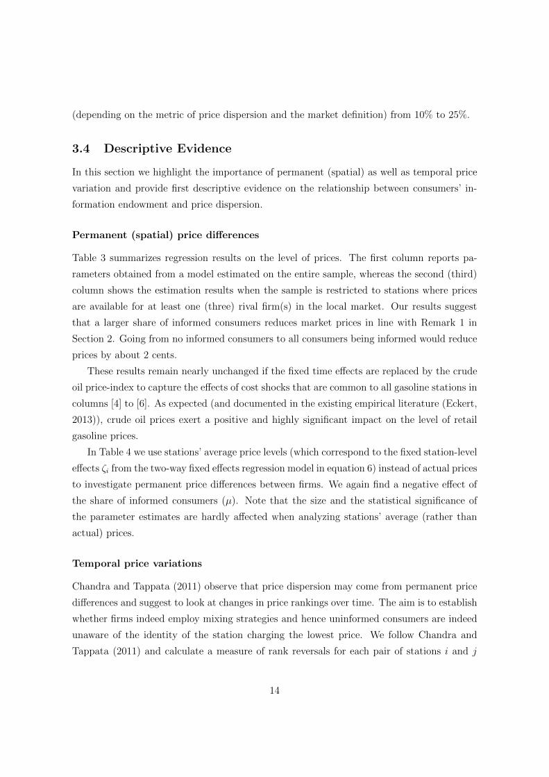
Table 3 summarizes regression results on the level of prices. The first column reports pa-

rameters obtained from a model estimated on the entire sample, whereas the second (third)

column shows the estimation results when the sample is restricted to stations where prices

are available for at least one (three) rival firm(s) in the local market. Our results suggest

that a larger share of informed consumers reduces market prices in line with Remark 1 in

Section 2. Going from no informed consumers to all consumers being informed would reduce

prices by about 2 cents.

These results remain nearly unchanged if the fixed time e↵ects are replaced by the crude

oil price-index to capture the e↵ects of cost shocks that are common to all gasoline stations in

columns [4] to [6]. As expected (and documented in the existing empirical literature (Eckert,

2013)), crude oil prices exert a positive and highly significant impact on the level of retail

gasoline prices.

In Table 4 we use stations’ average price levels (which correspond to the fixed station-level

e↵ects ⇣i

from the two-way fixed e↵ects regression model in equation 6) instead of actual prices

to investigate permanent price di↵erences between firms. We again find a negative e↵ect of

the share of informed consumers (µ). Note that the size and the statistical significance of

the parameter estimates are hardly a↵ected when analyzing stations’ average (rather than

actual) prices.

Temporal price variations

Chandra and Tappata (2011) observe that price dispersion may come from permanent price

di↵erences and suggest to look at changes in price rankings over time. The aim is to establish

whether firms indeed employ mixing strategies and hence uninformed consumers are indeed

unaware of the identity of the station charging the lowest price. We follow Chandra and

Tappata (2011) and calculate a measure of rank reversals for each pair of stations i and j

14

Table 2: Descriptive Statistics on Measures of Price Dispersion

Local market delineation 2 Miles 1.5 Miles MunicipalityMean S.D. Mean S.D. Mean S.D.

# of rival firms (N) 6.965 (6.415) 5.051 (4.126) 13.781 (19.145)# of rival firms with prices (N

o

) 4.428 (4.351) 3.346 (2.888) 7.919 (10.054)# of obs. 14,851 13,464 14,037Residual PricesV OIM 0.725 (0.781) 0.644 (0.721) 0.847 (0.902)V OI 0.723 (1.095) 0.643 (1.034) 0.847 (1.204)Range 1.467 (1.526) 1.306 (1.415) 1.725 (1.77)SDM 0.538 (0.546) 0.508 (0.542) 0.571 (0.556)AD 0.466 (0.608) 0.446 (0.59) 0.486 (0.632)

Raw PricesV OIM 0.747 (0.96) 0.655 (0.874) 0.9 (1.123)V OI 0.749 (1.355) 0.655 (1.264) 0.9 (1.536)Range 1.546 (2.028) 1.364 (1.88) 1.951 (2.513)SDM 0.538 (0.546) 0.541 (0.724) 0.652 (0.819)AD 0.498 (0.797) 0.471 (0.76) 0.548 (0.892)

Descriptive Statistics for Trimmed Range only:# of rival firms (N) 10.56 (6.769) 8.069 (4.233) 22.682 (21.662)# of rival firms with prices (N

o

) 7.03 (4.505) 5.66 (2.857) 13.035 (10.943)# of obs. 7,996 6,141 7,895Residual PricesTrimmed Range 0.881 (0.921) 0.753 (0.827) 1.21 (1.149)

Raw PricesTrimmed Range 0.879 (1.226) 0.746 (1.112) 1.255 (1.529)

Notes: Markets are restricted to having a minimum of one rival firm with priceinformation (N

o

� 1). For the trimmed range markets are restricted to three rivalfirms with price information (N

o

� 3).

15

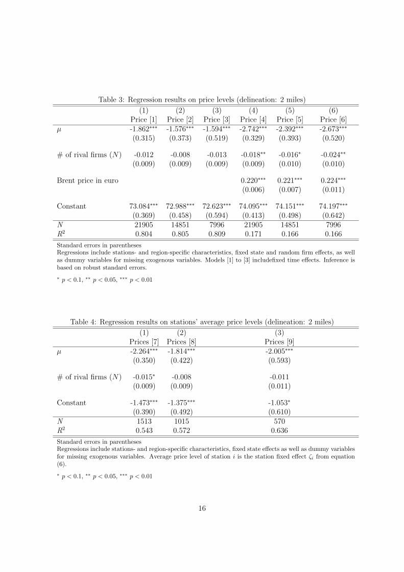
Table 3: Regression results on price levels (delineation: 2 miles)

(1) (2) (3) (4) (5) (6)Price [1] Price [2] Price [3] Price [4] Price [5] Price [6]

µ -1.862⇤⇤⇤ -1.576⇤⇤⇤ -1.594⇤⇤⇤ -2.742⇤⇤⇤ -2.392⇤⇤⇤ -2.673⇤⇤⇤

(0.315) (0.373) (0.519) (0.329) (0.393) (0.520)

# of rival firms (N) -0.012 -0.008 -0.013 -0.018⇤⇤ -0.016⇤ -0.024⇤⇤

(0.009) (0.009) (0.009) (0.009) (0.010) (0.010)

Brent price in euro 0.220⇤⇤⇤ 0.221⇤⇤⇤ 0.224⇤⇤⇤

(0.006) (0.007) (0.011)

Constant 73.084⇤⇤⇤ 72.988⇤⇤⇤ 72.623⇤⇤⇤ 74.095⇤⇤⇤ 74.151⇤⇤⇤ 74.197⇤⇤⇤

(0.369) (0.458) (0.594) (0.413) (0.498) (0.642)N 21905 14851 7996 21905 14851 7996R2 0.804 0.805 0.809 0.171 0.166 0.166

Standard errors in parenthesesRegressions include stations- and region-specific characteristics, fixed state and random firm e↵ects, as wellas dummy variables for missing exogenous variables. Models [1] to [3] includefixed time e↵ects. Inference isbased on robust standard errors.

⇤

p < 0.1, ⇤⇤

p < 0.05, ⇤⇤⇤

p < 0.01

Table 4: Regression results on stations’ average price levels (delineation: 2 miles)

(1) (2) (3)Prices [7] Prices [8] Prices [9]

µ -2.264⇤⇤⇤ -1.814⇤⇤⇤ -2.005⇤⇤⇤

(0.350) (0.422) (0.593)

# of rival firms (N) -0.015⇤ -0.008 -0.011(0.009) (0.009) (0.011)

Constant -1.473⇤⇤⇤ -1.375⇤⇤⇤ -1.053⇤

(0.390) (0.492) (0.610)N 1513 1015 570R2 0.543 0.572 0.636

Standard errors in parenthesesRegressions include stations- and region-specific characteristics, fixed state e↵ects as well as dummy variablesfor missing exogenous variables. Average price level of station i is the station fixed e↵ect ⇣

i

from equation(6).

⇤

p < 0.1, ⇤⇤

p < 0.05, ⇤⇤⇤

p < 0.01

16

(provided that i and j are located in the same local market and that we can observe prices

of both stations at least for two time periods). Let Tij

denote the number of periods where

price information of both firms are available. Subscripts i and j are assigned to the two

stations such that pit

� pjt

for most time periods. The measure of rank reversals is defined

as the proportion of observations with pjt

> pit

:

rij

=1

Tij

TijX

t=1

I{pjt>pit}, (7)

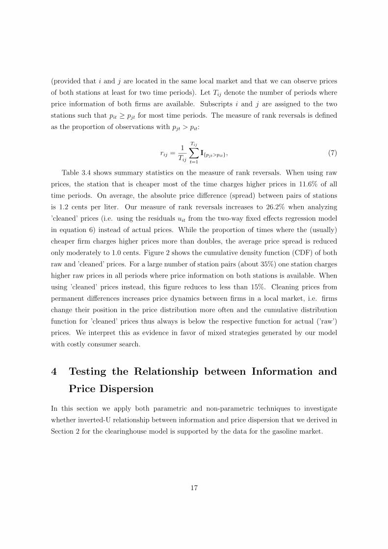
Table 3.4 shows summary statistics on the measure of rank reversals. When using raw

prices, the station that is cheaper most of the time charges higher prices in 11.6% of all

time periods. On average, the absolute price di↵erence (spread) between pairs of stations

is 1.2 cents per liter. Our measure of rank reversals increases to 26.2% when analyzing

’cleaned’ prices (i.e. using the residuals uit

from the two-way fixed e↵ects regression model

in equation 6) instead of actual prices. While the proportion of times where the (usually)

cheaper firm charges higher prices more than doubles, the average price spread is reduced

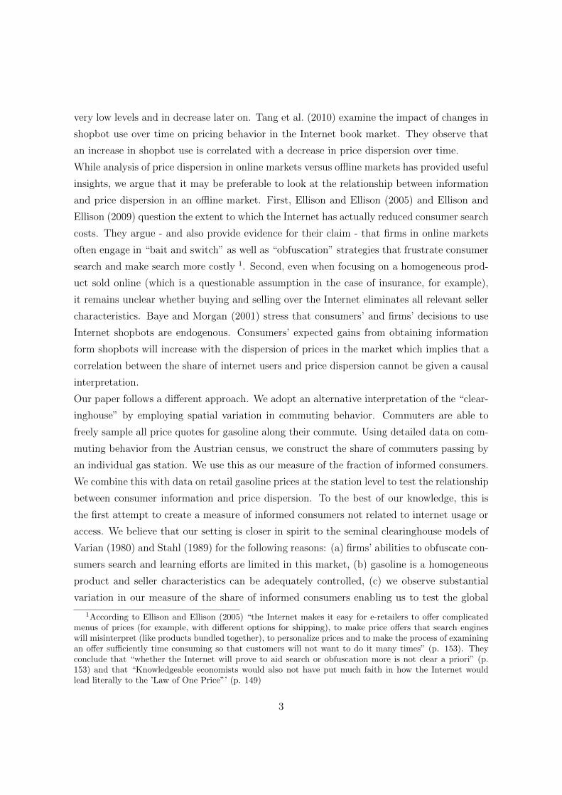
only moderately to 1.0 cents. Figure 2 shows the cumulative density function (CDF) of both

raw and ’cleaned’ prices. For a large number of station pairs (about 35%) one station charges

higher raw prices in all periods where price information on both stations is available. When

using ’cleaned’ prices instead, this figure reduces to less than 15%. Cleaning prices from

permanent di↵erences increases price dynamics between firms in a local market, i.e. firms

change their position in the price distribution more often and the cumulative distribution

function for ’cleaned’ prices thus always is below the respective function for actual (’raw’)

prices. We interpret this as evidence in favor of mixed strategies generated by our model

with costly consumer search.

4 Testing the Relationship between Information and

Price Dispersion

In this section we apply both parametric and non-parametric techniques to investigate

whether inverted-U relationship between information and price dispersion that we derived in

Section 2 for the clearinghouse model is supported by the data for the gasoline market.

17

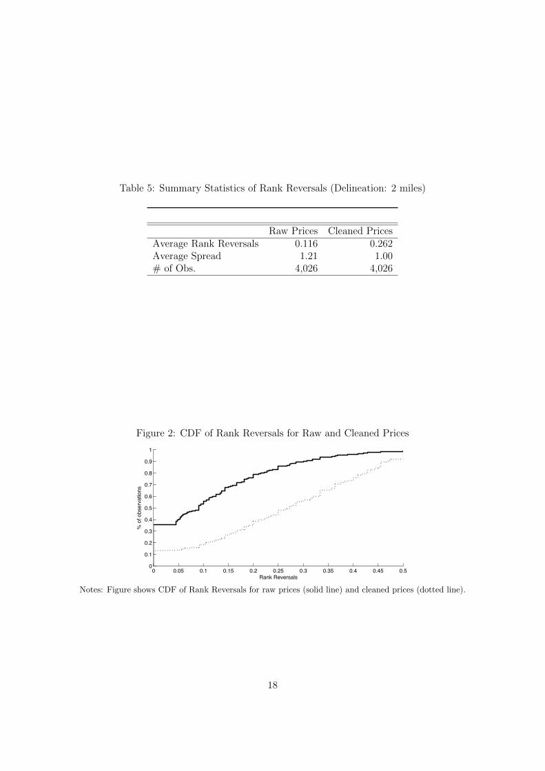
Table 5: Summary Statistics of Rank Reversals (Delineation: 2 miles)

Raw Prices Cleaned PricesAverage Rank Reversals 0.116 0.262Average Spread 1.21 1.00# of Obs. 4,026 4,026

Figure 2: CDF of Rank Reversals for Raw and Cleaned Prices

0 0.05 0.1 0.15 0.2 0.25 0.3 0.35 0.4 0.45 0.50

0.1

0.2

0.3

0.4

0.5

0.6

0.7

0.8

0.9

1

Rank Reversals

% o

f obs

erva

tions

Notes: Figure shows CDF of Rank Reversals for raw prices (solid line) and cleaned prices (dotted line).

18

4.1 Parametric Evidence

A straightforward approach to test for an inverse-U relationship between price dispersion

PDit

and the share of informed consumers (µi

) in station i’s market is to estimate the

following linear regression model:

PDit

= ↵ + �µi

+ �µ2i

+Xit

✓ + ⌘it

, (8)

where Xit

represents possible confounding factors at the station level as well as over

time. More specifically, we control for station-specific characteristics (such as brand name,

availability of service bay and/or convenience store, car wash facility, location) and region-

specific characteristics (such as population density, tra�c exposure of the station), as well

as measures characterizing the competitive environment (number of rivals in the market).

Further, period fixed e↵ects are included to remove price fluctuations that are common to

all gasoline stations.

The main parameters of interest are � and �. An inverted U-shaped relationship between

price dispersion and information, as predicted in Proposition 1, would imply that � > 0

and � < 0. According to the parameter estimates reported in Table 6, this proposition is

supported by the data in all specifications. While the size of the estimated coe�cients varies

between the models, the parameter estimates for � (�) are positive (negative) and statistically

significant at the 1%-significance level in all specifications based on the residual prices after

controlling for other confounding factors. As the share of informed consumers increases, price

dispersion first increases and then starts decreasing once the share of informed consumers

exceeds a critical level. The critical level implied by the parameter estimates lies between

between 0.70 and 0.76. As the share of informed consumers exceeds this level, the majority

of the stations attempts to capture the informed portion of the market which reduces price

dispersion.

To formally test for the presence of an inverted U-shaped relationship between information

and price dispersion, we apply the statistical test suggested in Lind and Mehlum (2010).13

This test calculates the slope of the estimation equation at both ends of the distribution of

the explanatory variable (µ). A positive slope for low values of the information measure and

a negative slope after a certain threshold (µ) would imply an inverted U-shaped relationship

between information and price dispersion. The test is an intersectionunion test as the null

13Lind and Mehlum (2010) argue that while a positive linear and a negative quadratic term supports aconcave relationship between two variables, it is not su�cient to guarantee an inverted-U shaped relationshipsince the relationship may be concave but still monotone in the relevant range.

19

hypothesis is that the parameter vector is contained in a union of specified sets. Results are

reported in Table 8. At the lower bound of our set of observations, the slope is positive and

significantly di↵erent from zero at the 1% level for all measures of price dispersion used. At

the upper bound the slope is negative in all specifications. The slope is significantly di↵erent

from zero at the 1% level (5% level) for the V OIM and the Trimmed Range measures (for

the V OI, Range, and AD measures) but is not significantly di↵erent from zero for the SDM

measure.

The regression results explaining price dispersion based on raw rather than residual prices

are summarized in Table 7. The qualitative results hardly change when using raw instead

of cleaned prices: The estimates of µ are positive and statistically significant in all model

specifications, while the parameter estimates on µ2 are negative for all measures of price

dispersion and statistically significant at the 5%-level (at the 10%-level) in five out of six (in

all) models.

When comparing the magnitude of our estimates of µ and µ2 across the models we find

that the (absolute values of the) parameters are largest for Range and Trimmed Range and

lowest for SD and SDM . This is due to the fact that Range and Trimmed Range are more

dispersed than SD and SDM , as the first two measures (and, to a lesser extent, V OI and

V OIM) will be more a↵ected by extreme values in the local price distribution. Further note

that the parameter estimates are slightly larger when analyzing raw prices (for the respective

measure of price dispersion), which also corresponds well to larger variances of measures of

price dispersion based on raw rather than cleaned prices.

The inverted-U shaped relationship between our measures of informed consumers and

price dispersion suggests that price dispersion is significantly smaller in markets where firms

are confronted mainly with either informed or uninformed consumers. For markets with an

intermediate information endowment of consumers, our findings clearly reject the ’law of one

price’.

In order to confirm that our results are not driven by the specific definition of market

boundaries, by particular sub-samples or by the chosen approach to calculate the measure

of information endowment µ, regressions were run using perturbations of these definitions:

First, in the sensitivity analysis the market delineation is based on smaller distances, on

administrative boundaries (municipalities) and on the consumers’ commuting behavior. Sec-

ond, we analyze sub-samples by excluding larger communities and by analyzing local markets

with at least three gasoline stations only. Last, we use the commuter flows to calculate µ

20

without weighting the flows by the number of possible routes.14 The main result of our anal-

ysis – an inverted-U shaped relationship between consumers’ information endowment and

price dispersion – remains una↵ected by these modifications. Results from these estimation

experiments are summarized in Appendix C..

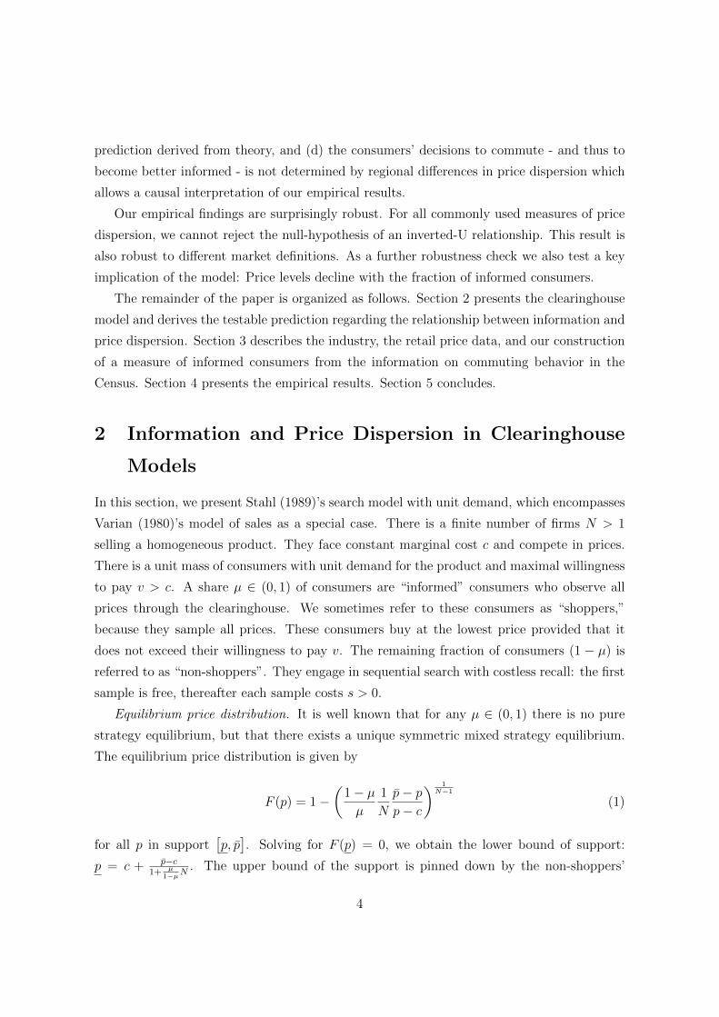
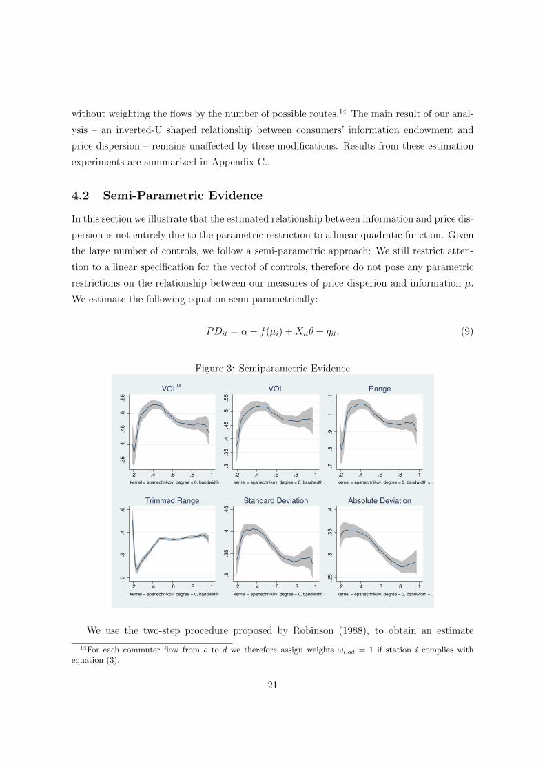
4.2 Semi-Parametric Evidence

In this section we illustrate that the estimated relationship between information and price dis-

persion is not entirely due to the parametric restriction to a linear quadratic function. Given

the large number of controls, we follow a semi-parametric approach: We still restrict atten-

tion to a linear specification for the vectof of controls, therefore do not pose any parametric

restrictions on the relationship between our measures of price disperion and information µ.

We estimate the following equation semi-parametrically:

PDit

= ↵ + f(µi

) +Xit

✓ + ⌘it

, (9)

Figure 3: Semiparametric Evidence

.35

.4.4

5.5

.55

.2 .4 .6 .8 1

kernel = epanechnikov, degree = 0, bandwidth = .07, pwidth = .1

VOI M

.3.3

5.4

.45

.5.5

5

.2 .4 .6 .8 1


VOI

.7.8

.91

1.1

.2 .4 .6 .8 1


Range

0.2

.4.6

.2 .4 .6 .8 1


Trimmed Range

.3.3

5.4

.45

.2 .4 .6 .8 1


Standard Deviation

.25

.3.3

5.4

.2 .4 .6 .8 1


Absolute Deviation

We use the two-step procedure proposed by Robinson (1988), to obtain an estimate

14For each commuter flow from o to d we therefore assign weights !

i,od

= 1 if station i complies withequation (3).

21

f(·). We first obtain nonparametric estimates of E(PD|µ) and E(X|µ) and then regress

PD � E(PD|µ) on X � E(X|µ) to obtain a consistent estimate of ✓. We then regress

E(PD|µ)�E(X|µ)✓ on µ non-parametrically to obtain an estimate of f(). Figure 3 reports

results obtained for the nonparametric component of regression equation 9 with a kernel-

weighted local polynomial regression. Although the specific form of the relationship between

price dispersion (shown on the vertical axis) and di↵erent measures of consumers’ information

(on the horizontal axis) di↵er across the measure of price disperion, there is strong evidence

in favor of an inverted U shape of the relationship of interest.

5 Conclusions

We have shown that a sequential search model where some consumers have access to the

realized prize distribution yields an inverted U relationship between price dispersion and the

fraction of informed consumers. Past studies have relied on internet usage or a comparison of

online and o✏ine markets to examine the e↵ect of informed consumers on prices. We provide

a novel measure of the fraction of informed consumers in the market for retail gasoline:

Commuters who can freely sample prices at gas stations along their commuting path. We

found robust statistical evidence supporting the information mechanism in clearinghouse

models. We also found that more informed consumers lower market prices. This may also be

related to our measure of information which -contrary to measures relating to the internet -

is less relevant for how di�cult monitoring is in a collusive setting.

22

References

Bahadir-Lust, S., Loy, J.-P., and Weiss, C. R. (2007). Are they always o↵ering the low-

est price? an empirical analysis of the persistence of price dispersion in a low inflation

environment. Managerial and Decision Economics, 28(7):777-788.

Barron, J. M., Taylor, B. A., and Umbeck, J. R. (2004). Number of sellers, average prices,

and price dispersion. International Journal of Industrial Organization, 22:1041-1066.

Baye, M. R. and Morgan, J. (2001). Information gatekeepers on the internet and the com-

petitiveness of homogeneous product markets. American Economic Review, 91(3):454-474.

Baye, M. R., Morgan, J., and Scholten, P. (2006). Information, search and price dispersion.

In Hendershott, T., editor, Economics and Information Systems, pages 323-377.

Brown, J. R. and Goolsbee, A. (2002). Does the internet make markets more competitive?

Evidence from the life insurance industry. Journal of Political Economy, 110(3):481-507.

Chandra, A. and Tappata, M. (2011). Consumer search and dynamic price dispersion: An

application to gasoline markets. The RAND Journal of Economics, 42(4):681-704.

Eckert, A. (2013). Empirical studies of gasoline retailing: A guide to the literature. Journal

of Economic Surveys, 27(1):140-166.

Ellison, G. and Ellison, S. F. (2005). Lessons about markets from the internet. Journal of

Economic Perspectives, 19(2):139-158.

Ellison, G. and Ellison, S. F. (2009). Search, obfuscation, and price elasticities on the internet.

Econometrica, 77(2):427-452.

Hastings, J. S. (2004). Vertical relationships and competition in retail gasoline markets:

Empirical evidence from contract changes in Southern California. American Economic

Review, 94(1):317-328.

Hosken, D. S., McMillan, R. S., and T.Taylor, C. (2008). Retail gasoline pricing: What do

we know? International Journal of Industrial Organization, 26(6):1425-1436.

Houde, J.-F. (2012). Spatial di↵erentiation and vertical mergers in retail markets for gasoline.

American Economic Review, 102(5):2147-2182.

23

Janssen, M., Pichler, P., and Weidenholzer, S. (2011). Oligopolistic markets with sequential

search and production cost uncertainty. The RAND Journal of Economics, 42(3):444–470.

Lach, S. (2002). Existence and persistence of price dispersion: An empirical analysis. Review

of Economics and Statistics, 84(3):433-444.

Lewis, M. (2008). Price dispersion and competition with spatially di↵erentiated sellers.

Journal of Industrial Economics, 56(3):654-678.

Lind, J. T. and Mehlum, H. (2010). With or without u? an appropriate test for a u-shaped

relationship. Oxford Bulletin of Economics and Statistics, 72(1):109-119.

Marvel, H. P. (1976). The economics of information and retail gasoline price behavior: An

empirical analysis. Journal of Political Economy, 84(5):1033-1060.

Robinson, P. M. (1988). Root-n-consistent semiparametric regression. Econometrica, pages

931-954.

Sorensen, A. T. (2000). Equilibrium price dispersion in retail markets for prescription drugs.

Journal of Political Economy, 108(4):833-850.

Stahl, D. O. (1989). Oligopolistic pricing with sequential consumer search. American Eco-

nomic Review, 79(4):700-712.

Statistik Austria (2006). Kfz-bestand 2005. available online at

http://www.statistik.at/web de/static/kfz-bestand 2005 021489.pdf, last accessed

19/07/2013.

Stigler, G. J. (1961). The economics of information. Journal of Political Economy, 69(3):213-

225.

Tang, Z., Smith, M. D., and Montgomery, A. (2010). The impact of shopbot use on prices and

price dispersion: Evidence from online book retailing. International Journal of Industrial

Organization, 28:579-590.

Tappata, M. (2009). Rockets and feathers: Understanding asymmetric pricing. The RAND

Journal of Economics, 40(4):673-687.

Teschl, G. (2012). Ordinary Di↵erential Equations and Dynamical Systems. American Math-

ematical Society.

Varian, H. R. (1980). A model of sales. American Economic Review, 70:651-659.

24

Appendix A. Proofs

Lemma 1. For all µ 2 (0, 1) and N � 2, let ↵(µ) =R 1

0dz

1+ µ1�µNz

N�1 . Then, µ 2 (0, 1) 7!

↵(µ)1�↵(µ) �

1�µ

µ

is strictly decreasing.

Proof. For all x > 0 and N � 2, let �(x) =R 1

0dz

1+xNz

N�1 , and notice that �(x) 2�

11+xN

, 1�.

Then, ↵(µ) = �⇣

µ

1�µ

⌘for all µ 2 (0, 1). Since µ

1�µ

is strictly increasing in µ, it follows that↵(µ)

1�↵(µ) �1�µ

µ

is strictly decreasing in µ on (0, 1) if and only if g(x) = �(x)1��(x) �

1x

is strictly

decreasing in x on (0,1).

Notice that for all x > 0,

�0(x) = �

Z 1

0

NzN�1

(1 + xNzN�1)2dz,

=1

x(N � 1)

✓1

1 + xN� �(x)

◆, (10)

where the second line is obtained by integrating by part. Therefore, if we define

�(y, x) =1

x(N � 1)

✓1

1 + xN� y

◆,

then � is a solution of di↵erential equation y0 = �(y, x) on interval (0,1).

For all x > 0, g0(x) = �

0(x)(1��(x))2 +

1x

2 . Using equation (10), we obtain that g0(x) is strictly

negative if and only if Px

(�(x)) < 0, where

Px

(Y ) = x (1� Y (1 + xN)) + (1� Y )2(N � 1)(1 + xN) 8X 2 R.

Px

(.) is strictly convex, and Px

(1) < 0 < Px

�1

1+xN

�. Therefore, there exists a unique

�(x) 2�

11+xN

, 1�such that P

x

(.) is strictly positive on�

11+xN

, �(x)�and strictly negative on

(�(x), 1). �(x) is given by

�(x) = 1 +x

2(N � 1)

1�

r1 +

4N(N � 1)

1 + xN

!.

Since �(x) 2�

11+xN

, 1�, it follows that g0(x) < 0 if and only if �(x) > �(x).

Next, let us show that �(x) > �(x) when x is in the neighborhood of 0, x > 0. Applying

Taylor’s theorem to �(x) for x ! 0+, we get:

�(x) = 1� x+2N2

2N � 1

x2

2�

6N3(1� 3N + 3N2)

(2N � 1)3x3

6+ o(x3),

25

where o(x3) is Landau’s small-o. Di↵erentiating � three times under the integral sign and

applying Taylor’s theorem for x ! 0+, we get:

�(x) = 1� x+2N2

2N � 1

x2

2�

6N3

3N � 2

x3

6+ o(x3).

It follows that

�(x)� �(x) = x3

✓N317N

3� 27N2 + 15N � 3

(2N � 1)3(3N � 2)+ o(1)

◆.

Since N3 17N3�27N2+15N�3(2N�1)3(3N�2) > 0 for all N � 2, there exists x0 > 0 such that �(x) � �(x) > 0

for all x 2 (0, x0].

Next, we show that �(x) � �(x) > 0 for all x > x0. We will establish this by showing

that � is a sub solution of di↵erential equation y0 = �(y, x) on [x0,1). � is a sub solution of

this di↵erential equation if and only if �0(x) < �(�(x), x) for all x � x0. �0(x)� �(�(x), x) is

given by

N

p(1 +Nx)(1 + 4N(N � 1) +Nx) ((x+ 2)N � 1)� (1 + 4N(N � 1) + 2N3x+N2x2)

2(N � 1)2(1 +Nx)p

(1 +Nx)(1 + 4N(N � 1) +Nx).

The above expression is strictly negative if and only if

(1 +Nx)(1 + 4N(N � 1) +Nx) ((x+ 2)N � 1)2 ��1 + 4N(N � 1) + 2N3x+N2x2

�2< 0.

The left-hand side is in fact equal to �4N2(N � 1)4x2, which is indeed strictly negative.

We can conclude: � is a solution of di↵erential equation y0 = �(y, x) on [x0,1), � is a

sub solution of the same di↵erential equation, and �(x0) > �(x0); by Lemma 1.2 in Teschl

(2012), �(x) > �(x) for all x > x0.

Appendix B. Weighting Commuter Flows

To calculate the number of potential routes we have to identify which stations are on the

same route. Two stations i and j that comply with equation (3) are on one route from o to

d if the optimal route between the two municipalities which passes through both stations is

not ”too much” longer than the optimal route from o to d passing through one station only.

The stations are ordered based on their distance from the origin. This implies that in the

equation below, the indexes i and j are assigned to these stations so that doi

doj

. Both

26

stations are on the same route if

distoi

+ distij

+ distjd

�min (distoi

+ distid

, distoj

+ distjd

) < dist (11)

with dij

as the optimal route between these two stations. Multiple stations are on the

same route if all pairs of stations comply with equation (11). If at least one station for a

particular commuter flow complies with equation (3) than each potential route contains at

least one station.15 Two potential routes between o and d are viewed as separate if at least

one station located on one route is not included in the other (and vice versa). The weight for a

commuter flow from o to d assigned to station i, !i,od

, equals the share of potential routes that

include station i (and equals zero if i does not comply with equation (3)). The aggregated

weighted number of transit commuters for station i is given by Ctr

i

=P

o

Pd 6=o

!i,od

Cod

, with

Cod

as the commuter flow from o to d.

Appendix C. Robustness

In this section of the Appendix we show the robustness of the findings reported in the main

part of the article by altering the model specification in various dimensions, namely (i) by the

way we delineate local markets, (ii) by analyzing sub-samples and (iii) by using a di↵erent

method to calculate the measure of information endowment µ.

As using a particular distance to delineate markets is rather arbitrary we use adminis-

trative boundaries (municipalities) and a di↵erent critical distance (1.5 instead of 2 miles)

to define local markets. The results on these alterations are reported in Table 9 and 10. In

all (all but one) model specifications the parameter estimates of µ (µ2) are positive (nega-

tive) and statistically di↵erent from zero at the 5%-significance level. The intersection union

test of Lind and Mehlum (2010) is rejected at the 5%-significance level for all measures of

price dispersion when market delineation is based on municipality boundaries, but only in

three (out of six) specifications when markets are defined using a critical distance of 1.5

miles. In the model specifications when the test fails to reject the null-hypothesis the peak

of the inverse-U appears rather late (at values of µ of about 0.75), leaving the downward-

sloping part at high levels of µ to be not statistically significant anymore. Nevertheless, the

concave relationship between information endowment and price dispersion is supported by

virtually all model specifications, while the inverse-U relationship is endorsed by 9 out of 12

specifications.

15We do not consider routes without stations when calculating these weights.

27

In addition to delineating local markets by (exogenously) chosen driving distances or by

administrative boundaries, we determine whether two stations are considered to be in the

same market by the share of common (potential) consumers, which we denote as relative

overlap (ROL). Two stations are considered to be within one local market if the share of

common (potential) consumers for both stations exceeds a certain threshold. Non-commuters

are considered to be potential consumers for both stations if both firms are located in the

same municipality. A commuter flow between o and d is considered to indicate potential

consumers for both firms if the commuter flow passes by both stations, i.e. both firms

comply with equation (3). The relative overlap between two stations i and j is defined as:

ROLij

=Cons

i

^ Consj

Consi

_ Consj

(12)

with Consi

(Consj

) as the number of potential consumers – including both commuters

and non-commuters – of station i (j). We again construct a local market for each station:

Station i’s market contains station i itself and all other stations j 6= i as long as ROLij

exceeds a particular critical value.

Table 11 summarizes the regression results when using a threshold-ROL of 50% to delin-

eate local markets. The parameter estimates of µ (µ2) are positive (negative) and statistically

significant, and the intersection union test is rejected at a 1%-significance level for all mea-

sures of price dispersion. The main results remain unchanged if we use low (high) threshold

levels for the ROL of 10% (90%). These results are not reported but are available from the

authors upon request.

In Table 12 and 13 we report regression results using sub-samples of the data. For the

model specifications summarized in Table 12 we exclude all stations located in the three

largest towns (besides Vienna), namely Graz, Linz and Salzburg, leaving only firms located

in municipalities with less than 120,000 inhabitants in the sample. We do so as our measure

of information is based on commuter flows at a municipality level, which is less precise in

very large towns. Evaluating this sub-sample hardly a↵ects the results, as reported in Table

12: All parameter estimates of µ and µ2 take the expected sign and are significantly di↵erent

from zero at the 1%-significance level. Additionally, the intersection union test is rejected at

the 1%-level in each specification.16

16We exclude stations located in Vienna throughout the analysis, as Vienna has more than 1.5 millioninhabitants and is therefore more than six times as large as the second biggest city. Our data on commutingbehavior within Vienna is therefore rather crude. However, including Vienna does not change the mainfindings: The parameter estimates of µ and µ

2 always take the expected sign and for all measures of dispersion(except the absolute distance (AD)) the parameter estimates of these variables are also significantly di↵erentfrom zero. These results are not reported, but are available from the authors upon request.

28

Additionally, we follow Chandra and Tappata (2011) and restrict our sample to stations

in local markets with three or more firms only (i.e. to stations with at least two competitors

where prices are observed in the particular period). These results are summarized in Table

13: Both the sign and the statistical significance of the parameter estimates of µ and µ2 as

well as the intersection union test support our main findings, that the relationship between

price dispersion and the share of informed consumers is characterized by an inverse-U.

In the last sensitivity analysis we refrain from weighting the commuter flows by the number

of potential routes when calculating the measure of information endowment µ. Technically,

when calculating the station i’s share of informed consumers, each commuter flow from

municipality o to community d gets a weight !i,od

= 1 if station i complies with equation

(3). Again, as summarized in Table 14, the parameter estimates of µ and µ2 take the

expected signs and are statistically significant at the 1%-significance level for each measure

of price dispersion. The intersection union test again supports the main finding of this article,

namely that consumers’ information endowment and price dispersion are characterized by an

inverted-U shaped relationship.

Appendix D. Tables

29

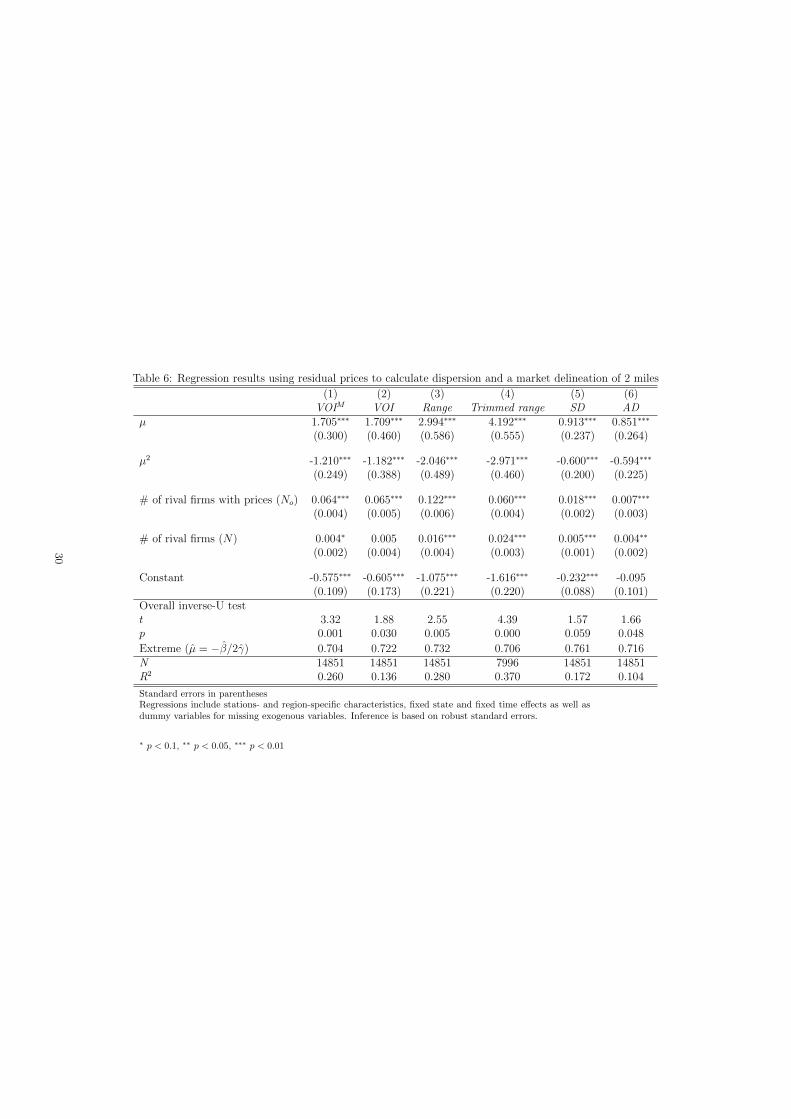
Table 6: Regression results using residual prices to calculate dispersion and a market delineation of 2 miles

(1) (2) (3) (4) (5) (6)VOIM VOI Range Trimmed range SD AD

µ 1.705⇤⇤⇤ 1.709⇤⇤⇤ 2.994⇤⇤⇤ 4.192⇤⇤⇤ 0.913⇤⇤⇤ 0.851⇤⇤⇤

(0.300) (0.460) (0.586) (0.555) (0.237) (0.264)

µ2 -1.210⇤⇤⇤ -1.182⇤⇤⇤ -2.046⇤⇤⇤ -2.971⇤⇤⇤ -0.600⇤⇤⇤ -0.594⇤⇤⇤

(0.249) (0.388) (0.489) (0.460) (0.200) (0.225)

# of rival firms with prices (No

) 0.064⇤⇤⇤ 0.065⇤⇤⇤ 0.122⇤⇤⇤ 0.060⇤⇤⇤ 0.018⇤⇤⇤ 0.007⇤⇤⇤

(0.004) (0.005) (0.006) (0.004) (0.002) (0.003)

# of rival firms (N) 0.004⇤ 0.005 0.016⇤⇤⇤ 0.024⇤⇤⇤ 0.005⇤⇤⇤ 0.004⇤⇤

(0.002) (0.004) (0.004) (0.003) (0.001) (0.002)

Constant -0.575⇤⇤⇤ -0.605⇤⇤⇤ -1.075⇤⇤⇤ -1.616⇤⇤⇤ -0.232⇤⇤⇤ -0.095(0.109) (0.173) (0.221) (0.220) (0.088) (0.101)

Overall inverse-U testt 3.32 1.88 2.55 4.39 1.57 1.66p 0.001 0.030 0.005 0.000 0.059 0.048Extreme (µ = ��/2�) 0.704 0.722 0.732 0.706 0.761 0.716N 14851 14851 14851 7996 14851 14851R2 0.260 0.136 0.280 0.370 0.172 0.104

Standard errors in parenthesesRegressions include stations- and region-specific characteristics, fixed state and fixed time e↵ects as well asdummy variables for missing exogenous variables. Inference is based on robust standard errors.

⇤

p < 0.1, ⇤⇤

p < 0.05, ⇤⇤⇤

p < 0.01

30

Table 7: Regression results using raw prices to calculate dispersion and a market delineation of 2 miles


µ 1.325⇤⇤⇤ 1.811⇤⇤⇤ 2.264⇤⇤⇤ 5.973⇤⇤⇤ 0.806⇤⇤ 0.992⇤⇤⇤

(0.382) (0.541) (0.796) (0.746) (0.323) (0.341)

µ2 -0.885⇤⇤⇤ -1.211⇤⇤⇤ -1.422⇤⇤ -4.370⇤⇤⇤ -0.504⇤ -0.692⇤⇤

(0.320) (0.462) (0.665) (0.621) (0.274) (0.290)


) 0.011⇤⇤⇤ 0.010⇤ 0.126⇤⇤⇤ 0.066⇤⇤⇤ 0.016⇤⇤⇤ 0.003(0.004) (0.006) (0.009) (0.006) (0.003) (0.003)

# of rival firms (N) 0.046⇤⇤⇤ 0.050⇤⇤⇤ 0.031⇤⇤⇤ 0.039⇤⇤⇤ 0.012⇤⇤⇤ 0.011⇤⇤⇤

(0.003) (0.004) (0.006) (0.004) (0.002) (0.003)

Constant -0.767⇤⇤⇤ -1.697⇤⇤⇤ -1.669⇤⇤⇤ -2.813⇤⇤⇤ -0.474⇤⇤⇤ -0.420⇤⇤⇤

(0.136) (0.205) (0.299) (0.292) (0.119) (0.133)Overall inverse-U testt 1.55 1.43 0.94 5.18 0.78 1.50p 0.061 0.076 0.172 0.000 0.219 0.067Extremum (µ = ��/2�) 0.749 0.748 0.796 0.683 0.800 0.716N 14851 14851 14851 7996 14851 14851R2 0.238 0.160 0.270 0.373 0.178 0.131


⇤

p < 0.1, ⇤⇤

p < 0.05, ⇤⇤⇤

p < 0.01

31

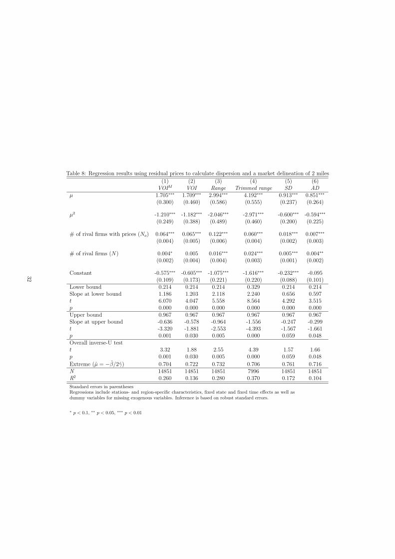
Table 8: Regression results using residual prices to calculate dispersion and a market delineation of 2 miles


µ 1.705⇤⇤⇤ 1.709⇤⇤⇤ 2.994⇤⇤⇤ 4.192⇤⇤⇤ 0.913⇤⇤⇤ 0.851⇤⇤⇤

(0.300) (0.460) (0.586) (0.555) (0.237) (0.264)

µ2 -1.210⇤⇤⇤ -1.182⇤⇤⇤ -2.046⇤⇤⇤ -2.971⇤⇤⇤ -0.600⇤⇤⇤ -0.594⇤⇤⇤

(0.249) (0.388) (0.489) (0.460) (0.200) (0.225)


) 0.064⇤⇤⇤ 0.065⇤⇤⇤ 0.122⇤⇤⇤ 0.060⇤⇤⇤ 0.018⇤⇤⇤ 0.007⇤⇤⇤

(0.004) (0.005) (0.006) (0.004) (0.002) (0.003)

# of rival firms (N) 0.004⇤ 0.005 0.016⇤⇤⇤ 0.024⇤⇤⇤ 0.005⇤⇤⇤ 0.004⇤⇤

(0.002) (0.004) (0.004) (0.003) (0.001) (0.002)

Constant -0.575⇤⇤⇤ -0.605⇤⇤⇤ -1.075⇤⇤⇤ -1.616⇤⇤⇤ -0.232⇤⇤⇤ -0.095(0.109) (0.173) (0.221) (0.220) (0.088) (0.101)

Lower bound 0.214 0.214 0.214 0.329 0.214 0.214Slope at lower bound 1.186 1.203 2.118 2.240 0.656 0.597t 6.070 4.047 5.558 8.564 4.292 3.515p 0.000 0.000 0.000 0.000 0.000 0.000Upper bound 0.967 0.967 0.967 0.967 0.967 0.967Slope at upper bound -0.636 -0.578 -0.964 -1.556 -0.247 -0.299t -3.320 -1.881 -2.553 -4.393 -1.567 -1.661p 0.001 0.030 0.005 0.000 0.059 0.048Overall inverse-U testt 3.32 1.88 2.55 4.39 1.57 1.66p 0.001 0.030 0.005 0.000 0.059 0.048Extreme (µ = ��/2�) 0.704 0.722 0.732 0.706 0.761 0.716N 14851 14851 14851 7996 14851 14851R2 0.260 0.136 0.280 0.370 0.172 0.104


⇤

p < 0.1, ⇤⇤

p < 0.05, ⇤⇤⇤

p < 0.01

32

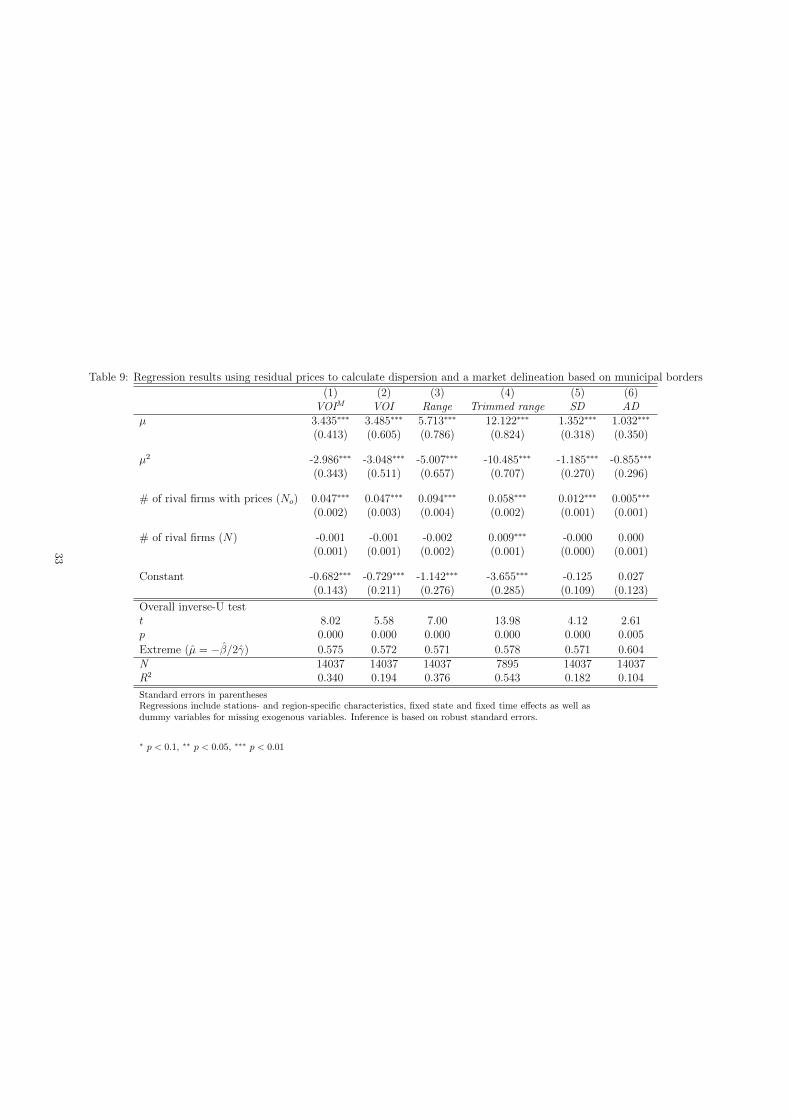
Table 9: Regression results using residual prices to calculate dispersion and a market delineation based on municipal borders


µ 3.435⇤⇤⇤ 3.485⇤⇤⇤ 5.713⇤⇤⇤ 12.122⇤⇤⇤ 1.352⇤⇤⇤ 1.032⇤⇤⇤

(0.413) (0.605) (0.786) (0.824) (0.318) (0.350)

µ2 -2.986⇤⇤⇤ -3.048⇤⇤⇤ -5.007⇤⇤⇤ -10.485⇤⇤⇤ -1.185⇤⇤⇤ -0.855⇤⇤⇤

(0.343) (0.511) (0.657) (0.707) (0.270) (0.296)


) 0.047⇤⇤⇤ 0.047⇤⇤⇤ 0.094⇤⇤⇤ 0.058⇤⇤⇤ 0.012⇤⇤⇤ 0.005⇤⇤⇤

(0.002) (0.003) (0.004) (0.002) (0.001) (0.001)

# of rival firms (N) -0.001 -0.001 -0.002 0.009⇤⇤⇤ -0.000 0.000(0.001) (0.001) (0.002) (0.001) (0.000) (0.001)

Constant -0.682⇤⇤⇤ -0.729⇤⇤⇤ -1.142⇤⇤⇤ -3.655⇤⇤⇤ -0.125 0.027(0.143) (0.211) (0.276) (0.285) (0.109) (0.123)



⇤

p < 0.1, ⇤⇤

p < 0.05, ⇤⇤⇤

p < 0.01

33

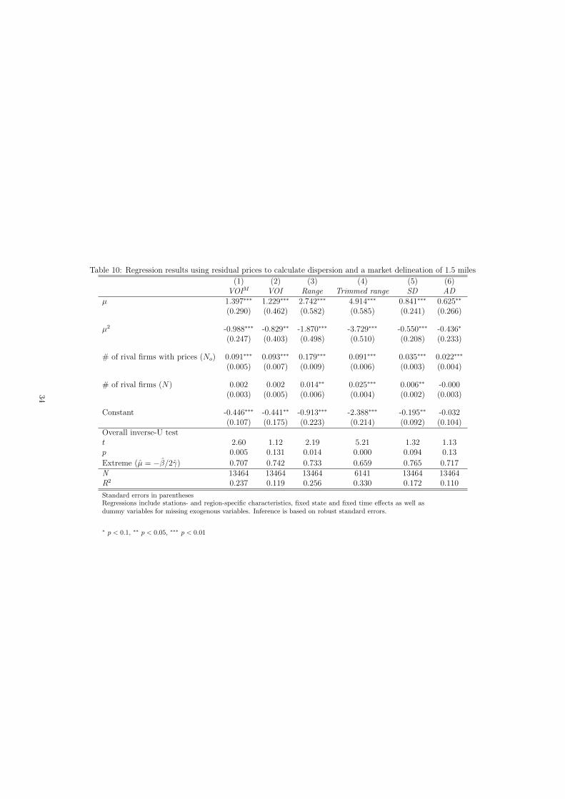
Table 10: Regression results using residual prices to calculate dispersion and a market delineation of 1.5 miles


µ 1.397⇤⇤⇤ 1.229⇤⇤⇤ 2.742⇤⇤⇤ 4.914⇤⇤⇤ 0.841⇤⇤⇤ 0.625⇤⇤

(0.290) (0.462) (0.582) (0.585) (0.241) (0.266)

µ2 -0.988⇤⇤⇤ -0.829⇤⇤ -1.870⇤⇤⇤ -3.729⇤⇤⇤ -0.550⇤⇤⇤ -0.436⇤

(0.247) (0.403) (0.498) (0.510) (0.208) (0.233)


) 0.091⇤⇤⇤ 0.093⇤⇤⇤ 0.179⇤⇤⇤ 0.091⇤⇤⇤ 0.035⇤⇤⇤ 0.022⇤⇤⇤

(0.005) (0.007) (0.009) (0.006) (0.003) (0.004)

# of rival firms (N) 0.002 0.002 0.014⇤⇤ 0.025⇤⇤⇤ 0.006⇤⇤ -0.000(0.003) (0.005) (0.006) (0.004) (0.002) (0.003)

Constant -0.446⇤⇤⇤ -0.441⇤⇤ -0.913⇤⇤⇤ -2.388⇤⇤⇤ -0.195⇤⇤ -0.032(0.107) (0.175) (0.223) (0.214) (0.092) (0.104)



⇤

p < 0.1, ⇤⇤

p < 0.05, ⇤⇤⇤

p < 0.01

34

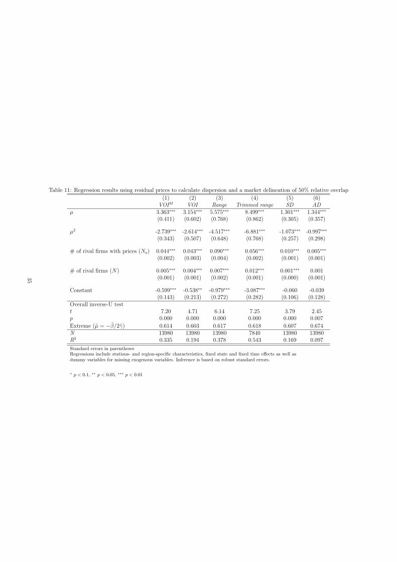
Table 11: Regression results using residual prices to calculate dispersion and a market delineation of 50% relative overlap


µ 3.363⇤⇤⇤ 3.154⇤⇤⇤ 5.575⇤⇤⇤ 8.499⇤⇤⇤ 1.301⇤⇤⇤ 1.344⇤⇤⇤

(0.411) (0.602) (0.768) (0.862) (0.305) (0.357)

µ2 -2.739⇤⇤⇤ -2.614⇤⇤⇤ -4.517⇤⇤⇤ -6.881⇤⇤⇤ -1.073⇤⇤⇤ -0.997⇤⇤⇤

(0.343) (0.507) (0.648) (0.768) (0.257) (0.298)


) 0.044⇤⇤⇤ 0.043⇤⇤⇤ 0.090⇤⇤⇤ 0.056⇤⇤⇤ 0.010⇤⇤⇤ 0.005⇤⇤⇤

(0.002) (0.003) (0.004) (0.002) (0.001) (0.001)

# of rival firms (N) 0.005⇤⇤⇤ 0.004⇤⇤⇤ 0.007⇤⇤⇤ 0.012⇤⇤⇤ 0.001⇤⇤⇤ 0.001(0.001) (0.001) (0.002) (0.001) (0.000) (0.001)

Constant -0.599⇤⇤⇤ -0.538⇤⇤ -0.979⇤⇤⇤ -3.087⇤⇤⇤ -0.060 -0.039(0.143) (0.213) (0.272) (0.282) (0.106) (0.128)



⇤

p < 0.1, ⇤⇤

p < 0.05, ⇤⇤⇤

p < 0.01

35

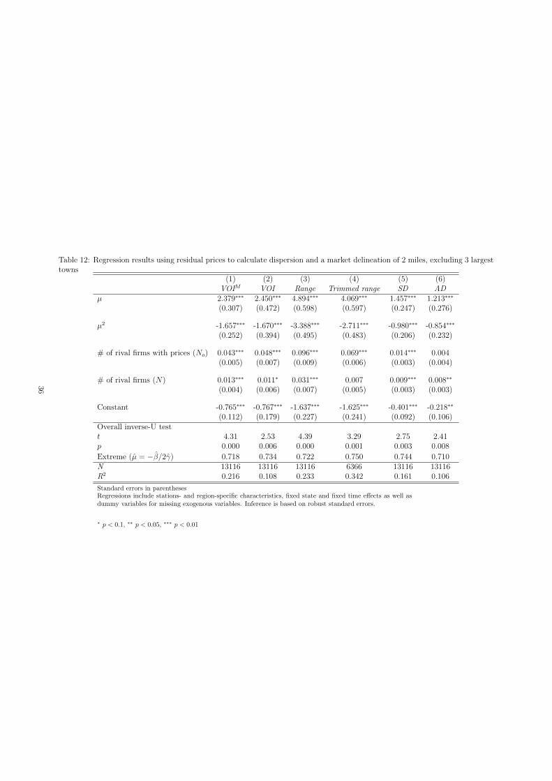
Table 12: Regression results using residual prices to calculate dispersion and a market delineation of 2 miles, excluding 3 largesttowns


µ 2.379⇤⇤⇤ 2.450⇤⇤⇤ 4.894⇤⇤⇤ 4.069⇤⇤⇤ 1.457⇤⇤⇤ 1.213⇤⇤⇤

(0.307) (0.472) (0.598) (0.597) (0.247) (0.276)

µ2 -1.657⇤⇤⇤ -1.670⇤⇤⇤ -3.388⇤⇤⇤ -2.711⇤⇤⇤ -0.980⇤⇤⇤ -0.854⇤⇤⇤

(0.252) (0.394) (0.495) (0.483) (0.206) (0.232)


) 0.043⇤⇤⇤ 0.048⇤⇤⇤ 0.096⇤⇤⇤ 0.069⇤⇤⇤ 0.014⇤⇤⇤ 0.004(0.005) (0.007) (0.009) (0.006) (0.003) (0.004)

# of rival firms (N) 0.013⇤⇤⇤ 0.011⇤ 0.031⇤⇤⇤ 0.007 0.009⇤⇤⇤ 0.008⇤⇤

(0.004) (0.006) (0.007) (0.005) (0.003) (0.003)

Constant -0.765⇤⇤⇤ -0.767⇤⇤⇤ -1.637⇤⇤⇤ -1.625⇤⇤⇤ -0.401⇤⇤⇤ -0.218⇤⇤

(0.112) (0.179) (0.227) (0.241) (0.092) (0.106)Overall inverse-U testt 4.31 2.53 4.39 3.29 2.75 2.41p 0.000 0.006 0.000 0.001 0.003 0.008Extreme (µ = ��/2�) 0.718 0.734 0.722 0.750 0.744 0.710N 13116 13116 13116 6366 13116 13116R2 0.216 0.108 0.233 0.342 0.161 0.106


⇤

p < 0.1, ⇤⇤

p < 0.05, ⇤⇤⇤

p < 0.01

36

Table 13: Results using residual prices and a market delineation of 2 miles, at least 2 competitors observed


µ 2.592⇤⇤⇤ 2.580⇤⇤⇤ 4.415⇤⇤⇤ 4.192⇤⇤⇤ 1.188⇤⇤⇤ 1.255⇤⇤⇤

(0.433) (0.664) (0.839) (0.555) (0.313) (0.375)

µ2 -1.893⇤⇤⇤ -1.861⇤⇤⇤ -3.121⇤⇤⇤ -2.971⇤⇤⇤ -0.801⇤⇤⇤ -0.939⇤⇤⇤

(0.356) (0.560) (0.694) (0.460) (0.260) (0.318)


) 0.052⇤⇤⇤ 0.054⇤⇤⇤ 0.099⇤⇤⇤ 0.060⇤⇤⇤ 0.010⇤⇤⇤ 0.002(0.004) (0.006) (0.007) (0.004) (0.002) (0.003)

# of rival firms (N) 0.008⇤⇤⇤ 0.008⇤⇤ 0.023⇤⇤⇤ 0.024⇤⇤⇤ 0.008⇤⇤⇤ 0.006⇤⇤⇤

(0.003) (0.004) (0.005) (0.003) (0.002) (0.002)

Constant -0.887⇤⇤⇤ -0.894⇤⇤⇤ -1.635⇤⇤⇤ -1.616⇤⇤⇤ -0.343⇤⇤⇤ -0.193(0.160) (0.256) (0.327) (0.220) (0.121) (0.149)



⇤

p < 0.1, ⇤⇤

p < 0.05, ⇤⇤⇤

p < 0.01

37

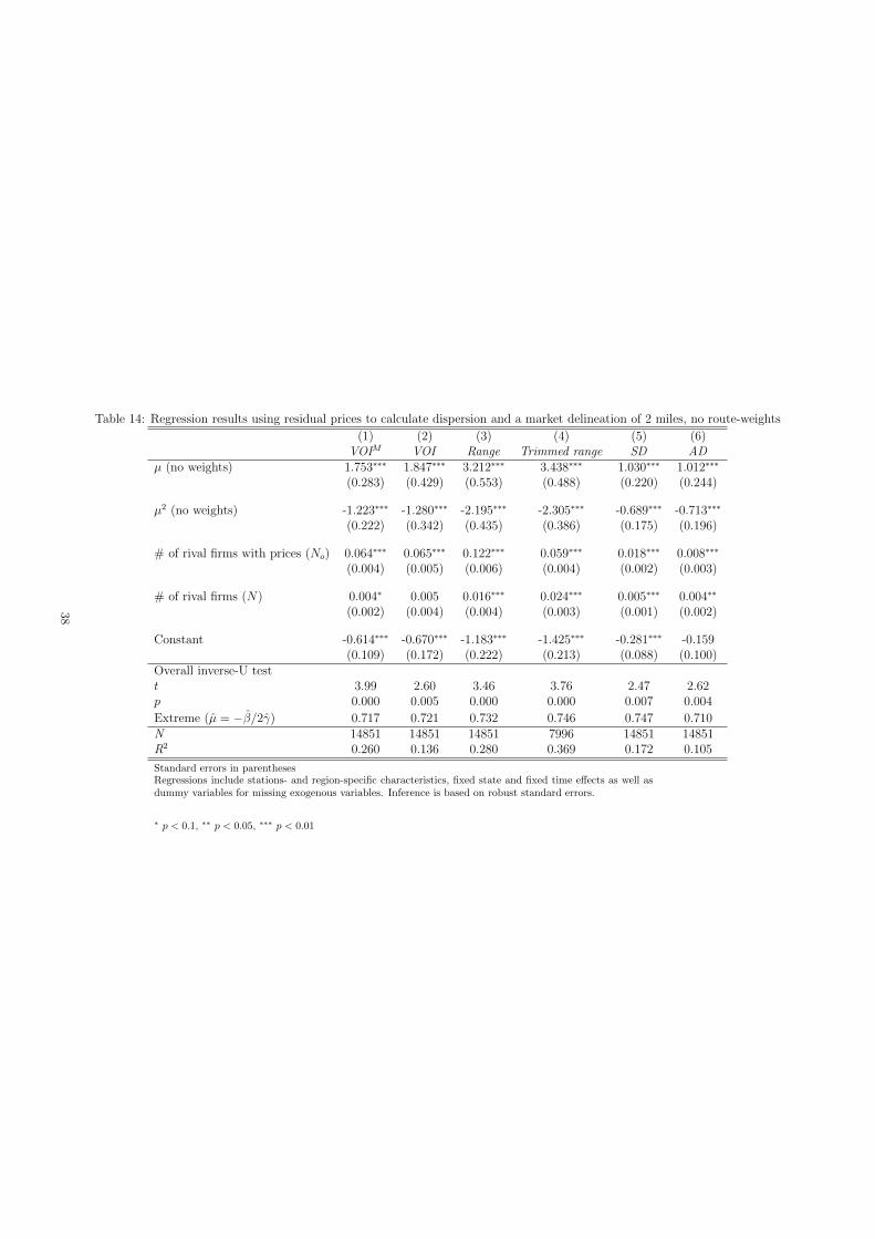
Table 14: Regression results using residual prices to calculate dispersion and a market delineation of 2 miles, no route-weights


µ (no weights) 1.753⇤⇤⇤ 1.847⇤⇤⇤ 3.212⇤⇤⇤ 3.438⇤⇤⇤ 1.030⇤⇤⇤ 1.012⇤⇤⇤

(0.283) (0.429) (0.553) (0.488) (0.220) (0.244)

µ2 (no weights) -1.223⇤⇤⇤ -1.280⇤⇤⇤ -2.195⇤⇤⇤ -2.305⇤⇤⇤ -0.689⇤⇤⇤ -0.713⇤⇤⇤

(0.222) (0.342) (0.435) (0.386) (0.175) (0.196)


) 0.064⇤⇤⇤ 0.065⇤⇤⇤ 0.122⇤⇤⇤ 0.059⇤⇤⇤ 0.018⇤⇤⇤ 0.008⇤⇤⇤

(0.004) (0.005) (0.006) (0.004) (0.002) (0.003)

# of rival firms (N) 0.004⇤ 0.005 0.016⇤⇤⇤ 0.024⇤⇤⇤ 0.005⇤⇤⇤ 0.004⇤⇤

(0.002) (0.004) (0.004) (0.003) (0.001) (0.002)

Constant -0.614⇤⇤⇤ -0.670⇤⇤⇤ -1.183⇤⇤⇤ -1.425⇤⇤⇤ -0.281⇤⇤⇤ -0.159(0.109) (0.172) (0.222) (0.213) (0.088) (0.100)



⇤

p < 0.1, ⇤⇤

p < 0.05, ⇤⇤⇤

p < 0.01

38

information and price dispersion: evidence from retail

Documents