INFORMATION AND COMMUNICATION

TECHNOLOGIES

(ICT)

PROGRAMME

Project FP7-ICT-2009-C-243881 CerCo

Report n. D2.1

Compiler design and intermediate languages

Version 1.0

Main Authors:Roberto M. Amadio, Nicolas Ayache, Yann Regis-Gianas,

Kayvan Memarian, Ronan Saillard

Project Acronym: CerCoProject full title: Certified ComplexityProposal/Contract no.: FP7-ICT-2009-C-243881 CerCo

1

CerCo, FP7-ICT-2009-C-243881 2

Abstract We discuss the problem of building a compiler which can lift in a provably correctway informations on the execution cost of the object code to cost annotations on the sourcecode. To this end, we need a clear and flexible picture of: (i) the meaning of cost annotations,(ii) the method to prove them sound and precise, and (iii) the way such proofs can be composed.We propose two approaches to these three questions which we name direct and labelling. Asa first step, we examine their application to a toy compiler. For this simple framework, weprovide a completely formal development which has been partly checked with the Coq proofassistant. This formal study suggests that the labelling approach, unlike the direct one, hasgood compositionality and scalability properties. In order to provide further evidence for thisclaim, we report our successful experience in implementing and testing the labelling approachon top of a prototype compiler written in ocaml for (a large fragment of) the C language.

CerCo, FP7-ICT-2009-C-243881 3

Contents

1 Introduction 51.1 Meaning of cost annotations . . . . . . . . . . . . . . . . . . . . . . . . . . . . . . . . . . . . . . 51.2 Soundness and precision of cost annotations . . . . . . . . . . . . . . . . . . . . . . . . . . . . . 61.3 Compositionality . . . . . . . . . . . . . . . . . . . . . . . . . . . . . . . . . . . . . . . . . . . . 61.4 Direct approach to cost annotations . . . . . . . . . . . . . . . . . . . . . . . . . . . . . . . . . 61.5 Labelling approach to cost annotations . . . . . . . . . . . . . . . . . . . . . . . . . . . . . . . . 71.6 A toy compiler . . . . . . . . . . . . . . . . . . . . . . . . . . . . . . . . . . . . . . . . . . . . . 81.7 A C compiler . . . . . . . . . . . . . . . . . . . . . . . . . . . . . . . . . . . . . . . . . . . . . . 81.8 Organisation . . . . . . . . . . . . . . . . . . . . . . . . . . . . . . . . . . . . . . . . . . . . . . 9

2 A toy compiler 92.1 Imp: language and semantics . . . . . . . . . . . . . . . . . . . . . . . . . . . . . . . . . . . . . 92.2 Big-step semantics . . . . . . . . . . . . . . . . . . . . . . . . . . . . . . . . . . . . . . . . . . . 92.3 Small-step semantics . . . . . . . . . . . . . . . . . . . . . . . . . . . . . . . . . . . . . . . . . . 102.4 Vm: language and semantics . . . . . . . . . . . . . . . . . . . . . . . . . . . . . . . . . . . . . . 112.5 Compilation from Imp to Vm . . . . . . . . . . . . . . . . . . . . . . . . . . . . . . . . . . . . . 122.6 Soundness of compilation for the big-step semantics . . . . . . . . . . . . . . . . . . . . . . . . 122.7 Soundness of compilation for the small-step semantics . . . . . . . . . . . . . . . . . . . . . . . 122.8 Compiled code is well-formed . . . . . . . . . . . . . . . . . . . . . . . . . . . . . . . . . . . . . 132.9 Mips: language and semantics . . . . . . . . . . . . . . . . . . . . . . . . . . . . . . . . . . . . . 132.10 Compilation from Vm to Mips . . . . . . . . . . . . . . . . . . . . . . . . . . . . . . . . . . . . . 14

3 Direct approach for the toy compiler 143.1 Mips and Vm cost annotations . . . . . . . . . . . . . . . . . . . . . . . . . . . . . . . . . . . . . 153.2 Imp cost annotation . . . . . . . . . . . . . . . . . . . . . . . . . . . . . . . . . . . . . . . . . . 163.3 Composition . . . . . . . . . . . . . . . . . . . . . . . . . . . . . . . . . . . . . . . . . . . . . . 173.4 Coq development . . . . . . . . . . . . . . . . . . . . . . . . . . . . . . . . . . . . . . . . . . . . 183.5 Limitations of the direct approach . . . . . . . . . . . . . . . . . . . . . . . . . . . . . . . . . . 18

4 Labelling approach for the toy compiler 184.1 Labelled Imp . . . . . . . . . . . . . . . . . . . . . . . . . . . . . . . . . . . . . . . . . . . . . . 184.2 Labelled Vm . . . . . . . . . . . . . . . . . . . . . . . . . . . . . . . . . . . . . . . . . . . . . . . 194.3 Labelled Mips . . . . . . . . . . . . . . . . . . . . . . . . . . . . . . . . . . . . . . . . . . . . . . 204.4 Labellings and instrumentations . . . . . . . . . . . . . . . . . . . . . . . . . . . . . . . . . . . 204.5 Sound and precise labellings . . . . . . . . . . . . . . . . . . . . . . . . . . . . . . . . . . . . . . 21

5 A C compiler 235.1 Clight . . . . . . . . . . . . . . . . . . . . . . . . . . . . . . . . . . . . . . . . . . . . . . . . . . 235.2 Cminor . . . . . . . . . . . . . . . . . . . . . . . . . . . . . . . . . . . . . . . . . . . . . . . . . . 235.3 RTLAbs . . . . . . . . . . . . . . . . . . . . . . . . . . . . . . . . . . . . . . . . . . . . . . . . . 235.4 RTL . . . . . . . . . . . . . . . . . . . . . . . . . . . . . . . . . . . . . . . . . . . . . . . . . . . 275.5 ERTL . . . . . . . . . . . . . . . . . . . . . . . . . . . . . . . . . . . . . . . . . . . . . . . . . . 275.6 LTL . . . . . . . . . . . . . . . . . . . . . . . . . . . . . . . . . . . . . . . . . . . . . . . . . . . 295.7 LIN . . . . . . . . . . . . . . . . . . . . . . . . . . . . . . . . . . . . . . . . . . . . . . . . . . . . 305.8 Mips . . . . . . . . . . . . . . . . . . . . . . . . . . . . . . . . . . . . . . . . . . . . . . . . . . . 30

6 Labelling approach for the C compiler 316.1 Labelled Clight and labelled Cminor . . . . . . . . . . . . . . . . . . . . . . . . . . . . . . . . . . 316.2 Labels in RTLAbs and the back-end languages . . . . . . . . . . . . . . . . . . . . . . . . . . . . 326.3 Labelling of the source language . . . . . . . . . . . . . . . . . . . . . . . . . . . . . . . . . . . 32

6.3.1 Sequential instructions . . . . . . . . . . . . . . . . . . . . . . . . . . . . . . . . . . . . . 326.3.2 Ternary expressions . . . . . . . . . . . . . . . . . . . . . . . . . . . . . . . . . . . . . . 326.3.3 Conditionals . . . . . . . . . . . . . . . . . . . . . . . . . . . . . . . . . . . . . . . . . . 336.3.4 Loops . . . . . . . . . . . . . . . . . . . . . . . . . . . . . . . . . . . . . . . . . . . . . . 336.3.5 Program Labels and Gotos . . . . . . . . . . . . . . . . . . . . . . . . . . . . . . . . . . 346.3.6 Function calls . . . . . . . . . . . . . . . . . . . . . . . . . . . . . . . . . . . . . . . . . . 34

CerCo, FP7-ICT-2009-C-243881 4

6.4 Verifications on the object code . . . . . . . . . . . . . . . . . . . . . . . . . . . . . . . . . . . . 356.5 Building the cost annotation . . . . . . . . . . . . . . . . . . . . . . . . . . . . . . . . . . . . . 356.6 Testing . . . . . . . . . . . . . . . . . . . . . . . . . . . . . . . . . . . . . . . . . . . . . . . . . 36

7 Conclusion and future work 36

A Proofs 38A.1 Notation . . . . . . . . . . . . . . . . . . . . . . . . . . . . . . . . . . . . . . . . . . . . . . . . . 38A.2 Proof of proposition 4 . . . . . . . . . . . . . . . . . . . . . . . . . . . . . . . . . . . . . . . . . 38A.3 Proof of proposition 8 . . . . . . . . . . . . . . . . . . . . . . . . . . . . . . . . . . . . . . . . . 39A.4 Proof of proposition 10 . . . . . . . . . . . . . . . . . . . . . . . . . . . . . . . . . . . . . . . . . 39A.5 Proof of proposition 11 . . . . . . . . . . . . . . . . . . . . . . . . . . . . . . . . . . . . . . . . . 40A.6 Proof of proposition 13 . . . . . . . . . . . . . . . . . . . . . . . . . . . . . . . . . . . . . . . . . 40A.7 Proof of proposition 14 . . . . . . . . . . . . . . . . . . . . . . . . . . . . . . . . . . . . . . . . . 40A.8 Proof of proposition 16 . . . . . . . . . . . . . . . . . . . . . . . . . . . . . . . . . . . . . . . . . 40A.9 Proof of proposition 17 . . . . . . . . . . . . . . . . . . . . . . . . . . . . . . . . . . . . . . . . . 40A.10 Proof of proposition 20 . . . . . . . . . . . . . . . . . . . . . . . . . . . . . . . . . . . . . . . . . 41A.11 Proof of proposition 22 . . . . . . . . . . . . . . . . . . . . . . . . . . . . . . . . . . . . . . . . . 41A.12 Proof of proposition 23 . . . . . . . . . . . . . . . . . . . . . . . . . . . . . . . . . . . . . . . . . 41A.13 Proof of proposition 25 . . . . . . . . . . . . . . . . . . . . . . . . . . . . . . . . . . . . . . . . . 41

CerCo, FP7-ICT-2009-C-243881 5

1 Introduction

The formal description and certification of software components is reaching a certain level ofmaturity with impressing case studies ranging from compilers to kernels of operating systems.A well-documented example is the proof of functional correctness of a moderately optimisingcompiler from a large subset of the C language to a typical assembly language of the kind usedin embedded systems [8].

In the framework of the Certified Complexity (CerCo) project [2], we aim to refine this lineof work by focusing on the issue of the execution cost of the compiled code. Specifically, we aimto build a formally verified C compiler that given a source program produces automaticallya functionally equivalent object code plus an annotation of the source code which is a soundand precise description of the execution cost of the object code.

We target in particular the kind of C programs produced for embedded applications; theseprograms are eventually compiled to binaries executable on specific processors. The currentstate of the art in commercial products such as Scade [3, 6] is that the reaction time of theprogram is estimated by means of abstract interpretation methods (such as those developedby AbsInt [1, 5]) that operate on the binaries. These methods rely on a specific knowledgeof the architecture of the processor and may require explicit annotations of the binaries todetermine the number of times a loop is iterated (see, e.g., [13] for a survey of the state of theart).

In this context, our aim is to produce a functionally correct compiler which can lift in aprovably correct way the pieces of information on the execution cost of the binary code to costannotations on the source C code. Eventually, we plan to manipulate the cost annotationswith automatic tools such as Frama− C [4].

In order to carry on our project, we need a clear and flexible picture of: (i) the meaningof cost annotations, (ii) the method to prove them sound and precise, and (iii) the way suchproofs can be composed. Our purpose here is to propose two methodologies addressing thesethree questions and to consider their concrete application to a simple toy compiler and to amoderately optimising C compiler.

1.1 Meaning of cost annotations

The execution cost of the source programs we are interested in depends on their controlstructure. Typically, the source programs are composed of mutually recursive procedures andloops and their execution cost depends, up to some multiplicative constant, on the number oftimes procedure calls and loop iterations are performed.

Producing a cost annotation of a source program amounts to:

• enrich the program with a collection of global cost variables to measure resource con-sumption (time, stack size, heap size,. . .)

• inject suitable code at some critical points (procedures, loops,. . .) to keep track of theexecution cost.

Thus producing a cost-annotation of a source program S amounts to build an annotatedprogram An(S) which behaves as S while self-monitoring its execution cost. In particular,if we do not observe the cost variables then we expect the annotated program An(S) to befunctionally equivalent to S. Notice that in the proposed approach an annotated program is

CerCo, FP7-ICT-2009-C-243881 6

a program in the source language. Therefore the meaning of the cost annotations is automat-ically defined by the semantics of the source language and tools developed to reason on thesource programs can be directly applied to the annotated programs too.

1.2 Soundness and precision of cost annotations

Suppose we have a functionally correct compiler C that associates with a program S in thesource language a program C(S) in the object language. Further suppose we have some obviousway of defining the execution cost of an object code. For instance, we have a good estimate ofthe number of cycles needed for the execution of each instruction of the object code. Now theannotation of the source program An(S) is sound if its prediction of the execution cost is anupper bound for the ‘real’ execution cost. Moreover, we say that the annotation is precise ifthe difference between the predicted and real execution costs is bounded by a constant whichdepends on the program.

1.3 Compositionality

In order to master the complexity of the compilation process (and its verification), the com-pilation function C must be regarded as the result of the composition of a certain number ofprogram transformations C = Ck ◦ · · · ◦ C1. When building a system of cost annotations ontop of an existing compiler a certain number of problems arise. First, the estimated cost ofexecuting a piece of source code is determined only at the end of the compilation process.Thus while we are used to define the compilation functions Ci in increasing order (from left toright), the annotation function An is the result of a progressive abstraction from the object tothe source code (from right to left). Second, we must be able to foresee in the source languagethe looping and branching points of the object code. Missing a loop may lead to unsound costannotations while missing a branching point may lead to rough cost predictions. This meansthat we must have a rather good idea of the way the source code will eventually be compiledto object code. Third, the definition of the annotation of the source code depends heavily oncontextual information. For instance, the cost of the compiled code associated with a simpleexpression such as x+ 1 will depend on the place in the memory hierarchy where the variablex is allocated.

1.4 Direct approach to cost annotations

A first ‘direct’ approach to the problem of building cost annotations is summarised by thefollowing diagram.

L1

An1

��

C1 // L2

An1

��

. . . Ck // Lk+1

Ank+1

��L1 L2 Lk+1

With respect to our previous discussion, L1 is the source language with the related an-notation function An1 while Lk+1 is the object language with a related annotation Ank+1.This annotation of the object code is supposed to be truly straightforward and it is taken asan ‘axiomatic’ definition of the ‘real’ execution cost of the program. The languages Li, for2 ≤ i ≤ k, are intermediate languages which are also equipped with increasingly ‘realistic’

CerCo, FP7-ICT-2009-C-243881 7

annotation functions. Suppose we denote with S the source program, with C(S) the compiledprogram, and that we write (P, s) ⇓ s′ to mean that the (source or object) program P inthe state s terminates successfully in the state s′. The soundness proof of the compilationfunction guarantees that if (S, s) ⇓ s′ then (C(S), s) ⇓ s′. In the direct approach, the proof ofsoundness of the cost annotations amounts to lift the proof of functional equivalence of thesource program and the object code to a proof of ‘quasi-equivalence’ of the respective instru-mented codes. Suppose we write s[c/cost ] for a state that associates c with the cost variablecost . Then what we want to show is that whenever (An1(S), s[c/cost ]) ⇓ s′[c′/cost ] we havethat (Ank+1(C(S)), s[d/cost ]) ⇓ s′[d′/cost ] and |d′ − d| ≤ |c′ − c| + k. This means that theincrement in the annotated source program bounds up to an additive constant the incrementin the annotated object program. We will also say that the cost annotation is precise if we canalso prove that |c′ − c| ≤ |d′ − d|, i.e., the ‘estimated’ cost is not too far away from the ‘real’one. We will see that while in theory one can build sound and precise annotation functions,in practice definitions and proofs become unwieldy.

1.5 Labelling approach to cost annotations

The ‘labelling’ approach to the problem of building cost annotations is summarized in thefollowing diagram.

L1

L1,`

I

OO

er1

C1 // L2,`

er2

��

. . . Ck // Lk+1,`

erk+1

��L1

L

II

C1 // L2 . . . Ck // Lk+1

er i+1 ◦ Ci = Ci ◦ er ier1 ◦ L = idL1

An1 = I ◦ L

For each language Li considered in the compilation process, we define an extended labelledlanguage Li,` and an extended operational semantics. The labels are used to mark certainpoints of the control. The semantics makes sure that whenever we cross a labelled controlpoint a labelled and observable transition is produced.

For each labelled language there is an obvious function er i erasing all labels and producing aprogram in the corresponding unlabelled language. The compilation functions Ci are extendedfrom the unlabelled to the labelled language so that they enjoy commutation with the erasurefunctions. Moreover, we lift the soundness properties of the compilation functions from theunlabelled to the labelled languages and transition systems.

A labelling L of the source language L1 is just a function such that erL1 ◦L is the identityfunction. An instrumentation I of the source labelled language L1,` is a function replacingthe labels with suitable increments of, say, a fresh cost variable. Then an annotation An1

of the source program can be derived simply as the composition of the labelling and theinstrumentation functions: An1 = I ◦ L.

As for the direct approach, suppose s is some adequate representation of the state of aprogram. Let S be a source program and suppose that its annotation satisfies the followingproperty:

(An1(S), s[c/cost ]) ⇓ s′[c+ δ/cost ] (1)

CerCo, FP7-ICT-2009-C-243881 8

where δ is some non-negative number. Then the definition of the instrumentation and thefact that the soundness proofs of the compilation functions have been lifted to the labelledlanguages allows to conclude that

(C(L(S)), s[c/cost ]) ⇓ (s′[c/cost ], λ) (2)

where C = Ck ◦ · · · ◦ C1 and λ is a sequence (or a multi-set) of labels whose ‘cost’ correspondsto the number δ produced by the annotated program. Then the commutation properties oferasure and compilation functions allows to conclude that the erasure of the compiled labelledcode erk+1(C(L(S))) is actually equal to the compiled code C(S) we are interested in. Giventhis, the following question arises:

Under which conditions the sequence λ, i.e., the increment δ, is a sound andpossibly precise description of the execution cost of the object code?

To answer this question, we observe that the object code we are interested in is some kindof assembly code and its control flow can be easily represented as a control flow graph. Thefact that we have to prove the soundness of the compilation functions means that we haveplenty of pieces of information on the way the control flows in the compiled code, in particularas far as procedure calls and returns are concerned. These pieces of information allow to builda rather accurate representation of the control flow of the compiled code at run time.

The idea is then to perform two simple checks on the control flow graph. The first check isto verify that all loops go through a labelled node. If this is the case then we can associate afinite cost with every label and prove that the cost annotations are sound. The second checkamounts to verify that all paths starting from a label have the same cost. If this check issuccessful then we can conclude that the cost annotations are precise.

1.6 A toy compiler

As a first case study for the two approaches to cost annotations we have sketched, we introducea toy compiler which is summarised by the following diagram.

ImpC // Vm

C′ // Mips

The three languages considered can be shortly described as follows: Imp is a very sim-ple imperative language with pure expressions, branching and looping commands, Vm is anassembly-like language enriched with a stack, and Mips is a Mips-like assembly language withregisters and main memory. The first compilation function C relies on the stack of the Vmlanguage to implement expression evaluation while the second compilation function C′ allo-cates (statically) the base of the stack in the registers and the rest in main memory. This isof course a naive strategy but it suffices to expose some of the problems that arise in defininga compositional approach (cf. section 1.3).

1.7 A C compiler

As a second, more complex, case study we consider a C compiler we have built in ocaml whosestructure is summarised by the following diagram:

C → Clight → Cminor → RTLAbs (front end)↓

Mips ← LIN ← LTL ← ERTL ← RTL (back-end)

CerCo, FP7-ICT-2009-C-243881 9

The structure follows rather closely the one of the CompCert compiler. Notable differencesare that some compilation steps are fusioned, that the front-end goes till RTLAbs (ratherthan Cminor) and that we target the Mips assembly language (rather than PowerPc). Thesedifferences are contingent to the way we built the compiler. The compilation from C to Clightrelies on the CIL front-end [11]. The one from Clight to RTL has been programmed from scratchand it is partly based on the Coq definitions available in the CompCert compiler. Finally,the back-end from RTL to Mips is based on a compiler developed in ocaml for pedagogicalpurposes [12]. The main optimisations it performs are common subexpression elimination,liveness analysis and register allocation, and graph compression.

1.8 Organisation

The rest of the paper is organised as follows. Section 2 describes the 3 languages and the 2compilation steps of the toy compiler. Section 3 describes the application of the direct approachto the toy compiler and points out its limitations. Section 4 describes the application of thelabelling approach to the toy compiler. Section 5 provides some details on the structure ofthe C compiler we have implemented. Section 6 reports our experience in implementing andtesting the labelling approach on the C compiler. Section 7 summarizes our contribution andoutlines some perspectives for future work. Section A sketches the proofs that have not beenmechanically checked in Coq.

2 A toy compiler

We formalise the toy compiler introduced in section 1.6.

2.1 Imp: language and semantics

The syntax of the Imp language is described below. This is a rather standard imperativelanguage with while loops and if-then-else.

id ::= x || y || . . . (identifiers)n ::= 0 || −1 || +1 || . . . (integers)v ::= n || true || false (values)e ::= id || n || e+ e (numerical expressions)b ::= e < e (boolean conditions)S ::= skip || id := e || S;S || if b then S else S || while b do S (commands)P ::= prog S (programs)

Let s be a total function from identifiers to integers representing the state. If s is a state,x an identifier, and n an integer then s[n/x] is the ‘updated’ state such that s[n/x](x) = nand s[n/x](y) = s(y) if x 6= y.

2.2 Big-step semantics

The big-step operational semantics of Imp programs is defined by the following judgements:

(e, s) ⇓ v (b, s) ⇓ v (S, s) ⇓ s′ (P, s) ⇓ s′

CerCo, FP7-ICT-2009-C-243881 10

(v, s) ⇓ v (x, s) ⇓ s(x)

(e, s) ⇓ v (e′, s) ⇓ v′(e+ e′, s) ⇓ (v +Z v

′)

(e, s) ⇓ v (e′, s) ⇓ v′(e < e′, s) ⇓ (v <Z v

′)

(skip, s) ⇓ s(e, s) ⇓ v

(x := e, s) ⇓ s[v/x]

(S1, s) ⇓ s′ (S2, s′) ⇓ s′′

(S1;S2, s) ⇓ s′′

(b, s) ⇓ true (S, s) ⇓ s′(if b then S else S′, s) ⇓ s′

(b, s) ⇓ false (S′, s) ⇓ s′(if b then S else S′, s) ⇓ s′

(b, s) ⇓ false

(while b do S, s) ⇓ s(b, s) ⇓ true (S;while b do S, s) ⇓ s′

(while b do S, s) ⇓ s′

(S, s) ⇓ s′(prog S, s) ⇓ s′

Table 1: Big-step operational semantics of Imp

(x := e,K, s) → (skip,K, s[v/x]) if (e, s) ⇓ v

(S;S′,K, s) → (S, S′ ·K, s)

(if b then S else S′,K, s) →{

(S,K, s) if (b, s) ⇓ true(S′,K, s) if (b, s) ⇓ false

(while b do S,K, s) →{

(S, (while b do S) ·K, s) if (b, s) ⇓ true(skip,K, s) if (b, s) ⇓ false

(skip, S ·K, s) → (S,K, s)

Table 2: Small-step operational semantics of Imp commands

and it is described in table 1. We assume that the addition v +Z v′ is only defined if v and

v′ are integers and the comparison v <Z v′ produces a value true or false only if v and v′ are

integers.

2.3 Small-step semantics

We also introduce an alternative small-step semantics of the Imp language. A continuation Kis a list of commands which terminates with a special symbol halt.

K ::= halt || S ·K

Table 2 defines a small-step semantics of Imp commands whose basic judgement has the shape:

(S,K, s)→ (S′,K ′, s′) .

We define the semantics of a program prog S as the semantics of the command S with con-tinuation halt. We derive a big step semantics from the small step one as follows:

(S, s) ⇓ s′ if (S, halt, s)→ · · · → (skip, halt, s′) .

CerCo, FP7-ICT-2009-C-243881 11

Rule C[i] =

C ` (i, σ, s)→ (i+ 1, n · σ, s) cnst(n)C ` (i, σ, s)→ (i+ 1, s(x) · σ, s) var(x)C ` (i, n · σ, s)→ (i+ 1, σ, s[n/x]) setvar(x)C ` (i, n · n′ · σ, s)→ (i+ 1, (n+Z n

′) · σ, s) add

C ` (i, σ, s)→ (i+ k + 1, σ, s) branch(k)C ` (i, n · n′ · σ, s)→ (i+ 1, σ, s) bge(k) and n <Z n

′

C ` (i, n · n′ · σ, s)→ (i+ k + 1, σ, s) bge(k) and n ≥Z n′

Table 3: Operational semantics Vm programs

2.4 Vm: language and semantics

Following [9], we define a virtual machine Vm and its programming language. The machineincludes the following elements: (1) A fixed code C (a possibly empty sequence of instructions),(2) A program counter pc, (3) A store s (as for the source program), (4) A stack of integers σ.

We will rely on the following instructions with the associated informal semantics:

cnst(n) push on the stackvar(x) push value xsetvar(x) pop value and assign it to xadd pop 2 values and push their sumbranch(k) jump with offset kbge(k) pop 2 values and jump if greater or equal with offset khalt stop computation

In the branching instructions, k is an integer that has to be added to the current programcounter in order to determine the following instruction to be executed. Given a sequence C,we denote with |C| its length and with C[i] its ith element (the leftmost element being the 0th

element). The operational semantics of the instructions is formalised by rules of the shape:

C ` (i, σ, s)→ (j, σ′, s′)

and it is fully described in table 3. Notice that Imp and Vm semantics share the same notionof store. We write, e.g., n · σ to stress that the top element of the stack exists and is n. Wewill also write (C, s) ⇓ s′ if C ` (0, ε, s)

∗→ (i, ε, s′) and C[i] = halt.Code coming from the compilation of Imp programs has specific properties that are used

in the following compilation step when values on the stack are allocated either in registers orin main memory. In particular, it turns out that for every instruction of the compiled codeit is possible to predict statically the height of the stack whenever the instruction is executed.We now proceed to define a simple notion of well-formed code and show that it enjoys thisproperty. In the following section, we will define the compilation function from Imp to Vmand show that it produces well-formed code.

Definition 1 We say that a sequence of instructions C is well formed if there is a functionh : {0, . . . , |C|} → N which satisfies the conditions listed in table 4 for 0 ≤ i ≤ |C|− 1. In thiscase we write C : h.

The conditions defining the predicate C : h are strong enough to entail that h correctlypredicts the stack height and to guarantee the uniqueness of h up to the initial condition.

Proposition 2 (1) If C : h, C ` (i, σ, s)∗→ (j, σ′, s′), and h(i) = |σ| then h(j) = |σ′|.

(2) If C : h, C : h′ and h(0) = h′(0) then h = h′.

CerCo, FP7-ICT-2009-C-243881 12

C[i] = Conditions for C : h

cnst(n) or var(x) h(i+ 1) = h(i) + 1add h(i) ≥ 2, h(i+ 1) = h(i)− 1setvar(x) h(i) = 1, h(i+ 1) = 0branch(k) 0 ≤ i+ k + 1 ≤ |C|, h(i) = h(i+ 1) = h(i+ k + 1) = 0bge(k) 0 ≤ i+ k + 1 ≤ |C|, h(i) = 2, h(i+ 1) = h(i+ k + 1) = 0halt i = |C| − 1, h(i) = h(i+ 1) = 0

Table 4: Conditions for well-formed code

C(x) = var(x) C(n) = cnst(n) C(e+ e′) = C(e) · C(e′) · add

C(e < e′, k) = C(e) · C(e′) · bge(k)

C(x := e) = C(e) · setvar(x) C(S;S′) = C(S) · C(S′)

C(if b then S else S′) = C(b, k) · C(S) · (branch(k′)) · C(S′)where: k = sz (S) + 1, k′ = sz (S′)

C(while b do S) = C(b, k) · C(S) · branch(k′)where: k = sz (S) + 1, k′ = −(sz (b) + sz (S) + 1)

C(prog S) = C(S) · halt

Table 5: Compilation from Imp to Vm

2.5 Compilation from Imp to Vm

In table 5, we define compilation functions C from Imp to Vm which operate on expressions,boolean conditions, statements, and programs. We write sz (e), sz (b), sz (S) for the number ofinstructions the compilation function associates with the expression e, the boolean conditionb, and the statement S, respectively.

2.6 Soundness of compilation for the big-step semantics

We follow [9] for the proof of correctness of the compilation function with respect to thebig-step semantics (see also [10] for a much older reference).

Proposition 3 The following properties hold:

(1) If (e, s) ⇓ v then C · C(e) · C ′ ` (i, σ, s)∗→ (j, v · σ, s) where i = |C| and j = |C · C(e)|.

(2) If (b, s) ⇓ true then C ·C(b, k)·C ′ ` (i, σ, s)∗→ (j+k, σ, s) where i = |C| and j = |C ·C(b, k)|.

(3) If (b, s) ⇓ false then C · C(b, k) ·C ′ ` (i, σ, s)∗→ (j, σ, s) where i = |C| and j = |C · C(b, k)|.

(4) If (S, s) ⇓ s′ then C · C(S) · C ′ ` (i, σ, s)∗→ (j, σ, s′) where i = |C| and j = |C · C(e)|.

2.7 Soundness of compilation for the small-step semantics

We prove soundness with respect to the small step semantics too. To this end, given a Vm

code C, we define an ‘accessibility relation’C; as the least binary relation on {0, . . . , |C| − 1}

such that:

CerCo, FP7-ICT-2009-C-243881 13

iC; i

C[i] = branch(k) (i+ k + 1)C; j

iC; j

We also introduce a ternary relation R(C, i,K) which relates a Vm code C, a numberi ∈ {0, . . . , |C| − 1} and a continuation K. The intuition is that relative to the code C, theinstruction i can be regarded as having continuation K. Formally, the relation R is definedas the least one that satisfies the following conditions.

iC; j C[j] = halt

R(C, i, halt)

iC; i′ C = C1 · C(S) · C2

i′ = |C1| j = |C1 · C(S)| R(C, j,K)

R(C, i, S ·K)

.

We can then state the correctness of the compilation function as follows.

Proposition 4 If (S,K, s)→ (S′,K ′, s′) and R(C, i, S ·K) then C ` (i, σ, s)∗→ (j, σ, s′) and

R(C, j, S′ ·K ′).

2.8 Compiled code is well-formed

As announced, we can prove that the result of the compilation is a well-formed code.

Proposition 5 For any expression e, statement S, and program P the following holds:

(1) For any n ∈ N there is a unique h such that C(e) : h, h(0) = n, and h(|C(e)|) = h(0) + 1.

(2) For any S, there is a unique h such that C(S) : h, h(0) = 0, and h(|C(e)|) = 0.

(3) There is a unique h such that C(P ) : h.

2.9 Mips: language and semantics

We consider a Mips-like machine [7] which includes the following elements: (1) a fixed codeM (a sequence of instructions), (2) a program counter pc, (3) a finite set of registers includingthe registers A, B, and R0, . . . , Rb−1, and (4) an (infinite) main memory which maps locationsto integers.

We denote with R,R′, . . . registers, with l, l′, . . . locations and with m,m′, . . . memorieswhich are total functions from registers and locations to (unbounded) integers. We will relyon the following instructions with the associated informal semantics:

loadi R,n store value n in the register Rload R, l store contents of location l in the register Rstore R, l store contents of register R in the location ladd R,R′, R′′ add contents of R′, R′′ and store it in Rbranch k jump with offset kbge R,R′, k jump with offset k if contents R greater or equal than contents R′

halt stop computation

We denote with M a list of instructions. The operational semantics is formalised in table6 by rules of the shape:

M ` (i,m)→ (j,m′)

where M is a list of Mips instructions, i, j are natural numbers and m,m′ are memories. Wewrite (M,m) ⇓ m′ if M ` (0,m)

∗→ (j,m′) and M [j] = halt.

CerCo, FP7-ICT-2009-C-243881 14

Rule M [i] =

M ` (i,m)→ (i+ 1,m[n/R]) loadi R,nM ` (i,m)→ (i+ 1,m[m(l)/R]) load R, lM ` (i,m)→ (i+ 1,m[m(R)/l])) store R, lM ` (i,m)→ (i+ 1,m[m(R′) +m(R′′)/R]) add R,R′, R′′

M ` (i,m)→ (i+ k + 1,m) branch kM ` (i,m)→ (i+ 1,m) bge R,R′, k and m(R) <Z m(R′)M ` (i,m)→ (i+ k + 1,m) bge R,R′, k and m(R) ≥Z m(R′)

Table 6: Operational semantics Mips programs

2.10 Compilation from Vm to Mips

In order to compile Vm programs to Mips programs we make the following hypotheses. (1)For every Vm program variable x we reserve an address lx, (2) For every natural numberh ≥ b, we reserve an address lh (the addresses lx, lh, . . . are all distinct), (3) We store thefirst b elements of the stack σ in the registers R0, . . . , Rb−1 and the remaining (if any) at theaddresses lb, lb+1, . . ..

We say that the memory m represents the stack σ and the store s, and write m ‖−σ, s, ifthe following conditions are satisfied: (1) s(x) = m(lx), and (2) if 0 ≤ i < |σ| then

σ[i] =

{m(Ri) if i < bm(li) if i ≥ b

The compilation function C′ from Vm to Mips is described in table 7. It operates on a well-formed Vm code C whose last instruction is halt. Hence, by proposition 5(3), there is a uniqueh such that C : h. We denote with C′(C) the concatenation C′(0, C) · · · C′(|C|−1, C). Given awell formed Vm code C with i < |C| we denote with p(i, C) the position of the first instructionin C′(C) which corresponds to the compilation of the instruction with position i in C. This isdefined as:1

p(i, C) = Σ0≤j<id(i, C), (3)

where the function d(i, C) is defined as follows:

d(i, C) = |C′(i, C)| . (4)

Hence d(i, C) is the number of Mips instructions associated with the ith instruction of the(well-formed) C code.

The functional correctness of the compilation function can then be stated as follows.

Proposition 6 Let C : h be a well formed code. If C ` (i, σ, s) → (j, σ′, s′) with h(i) = |σ|and m ‖−σ, s then C′(C) ` (p(i, C),m)

∗→ (p(j, C),m′) and m′ ‖−σ′, s′.

3 Direct approach for the toy compiler

We apply the direct approach discussed in section 1.4 to the toy compiler which results in thefollowing diagram:

1There is an obvious circularity in this definition that can be easily eliminated by defining first the functiond following the case analysis in table 7, then the function p as in (3), and finally the function C′ as in table 7.

CerCo, FP7-ICT-2009-C-243881 15

C[i] = C′(i, C) =

cnst(n)

{(loadi Rh, n) if h = h(i) < b(loadi A,n) · (store A, lh) otherwise

var(x)

{(load Rh, lx) if h = h(i) < b(load A, lx) · (store A, lh) otherwise

add

(add Rh−2, Rh−2, Rh−1) if h = h(i) < (b− 1)(load A, lh−1) · (add Rh−2, Rh−2, A) if h = h(i) = (b− 1)(load A, lh−1) · (load B, lh−2) if h = h(i) > (b− 1)(add A,B,A) · (store A, lh−2)

setvar(x)

{(store Rh−1 lx) if h = h(i) < b(load A, lh−1) · (store A, lx) if h = h(i) ≥ b

branch(k) (branch k′) if k′ = p(i+ k + 1, C)− p(i+ 1, C)

bge(k)

(bge Rh−2, Rh−1, k

′) if h = h(i) < (b− 1)(load A, lh−1) · (bge Rh−2, A, k

′) if h = h(i) = (b− 1)(load A, lh−2) · (load B, lh−1) · (bge A,B, k′) if h = h(i) > (b− 1) and

k′ = p(i+ k + 1, C)− p(i+ 1, C)

halt halt

Table 7: Compilation from Vm to Mips

ImpC //

AnImp

��

VmC′ //

AnVm

��

Mips

AnMips

��Imp Vm Mips

3.1 Mips and Vm cost annotations

The definition of the cost annotation AnMips(M) for a Mips code M goes as follows assumingthat all the Mips instructions have cost 1.

1. We select fresh locations lcost , lA, lB not used in M .

2. Before each instruction in M we insert the following list of 8 instructions whose effect isto increase by 1 the contents of location lcost :

(store A, lA) · (store B, lB) · (loadi A, 1) · (load B, lcost)·(add A,A,B) · (store A, lcost) · (load A, lA) · (load B, lB) .

3. We update the offset of the branching instructions according to the map k 7→ (9 · k).

The definition of the cost annotation AnVm(C) for a well-formed Vm code C such thatC : h goes as follows.

1. We select a fresh cost variable not used in C.

CerCo, FP7-ICT-2009-C-243881 16

C[i] = cnst(n) or var(x) add setvar(x) branch(k) bge(k) halt

κ(C[i]) = 2 4 2 1 3 1

Table 8: Upper bounds on the cost of Vm instructions

2. Before the instruction ith in C, we insert the following list of 4 instructions whose effect isto increase the cost variable by the maximum number κ(C[i]) of instructions associatedwith C[i] (as specified in table 8):

(cnst(κ(C[i]))) · (var(cost)) · (add) · (setvar(cost)) .

3. We update the offset of the branching instructions according to the map k 7→ (5 · k).

To summarise, the situation is that the instruction i of the Vm code C corresponds to: theinstruction 5 · i + 4 of the annotated Vm code AnVm(C), the instruction p(i, C) of the Mipscode C′(C), and the instruction 9 · p(i, C) + 8 of the instrumented Mips code AnMips(C′(C)).

The following lemma describes the effect of the injected sequences of instructions.

Lemma 7 The following properties hold:

(1) If M is a Mips instruction then C1 ·AnMips(M) ·C2 ` (|C1|,m[c/lcost ])∗→ (|C1|+ 8,m[c+

1/lcost ,m(A)/lA,m(B)/lB]).

(2) If C is a Vm instruction then C1 ·AnVm(C) ·C2 ` (|C1|, σ, s[c/cost ])∗→ (|C1|+ 4, σ, s[c+

κ(C[i])/cost ]), where i = |C1|.

The simulation proposition 6 is extended to the annotated codes as follows where we write→k for the relation obtained by composing k times the reduction relation →.

Proposition 8 Let C : h be a well-formed code. If AnVm(C) ` (5 · i, σ, s) →5 (5 · j, σ′, s′),m ‖−σ, s, and h(i) = |σ| then AnMips(C′(C)) ` (9 · p(i, C),m)

∗→ (9 · p(j, C),m′), withm′[s′(cost)/lcost ] ‖−σ′, s′ and

m′(lcost)−m(lcost) ≤ s′(cost)− s(cost) .

3.2 Imp cost annotation

The definition of the cost annotation An Imp(P ) for an Imp program P is defined in table 9 andit relies on an auxiliary function κ which provides an upper bound on the cost of executingthe various operators of the language. For the sake of simplicity, this annotation introducestwo main approximations:

• It over-approximates the cost of an if then else by taking the maximum cost of the costof the two branches.

• It always considers the worst case where the data in the stack resides in the main memory.

We will discuss in section 3.5 to what extent these approximations can be removed.Next we formulate the soundness of the Imp annotation with respect to the Vm annotation

along the pattern of proposition 3.

CerCo, FP7-ICT-2009-C-243881 17

An Imp(prog S) = cost := cost + κ(S);An Imp(S)An Imp(skip) = skipAn Imp(x := e) = x := eAn Imp(S;S′) = An Imp(S);An Imp(S

′)An Imp(if b then S else S′) = (if b then An Imp(S)

else An Imp(S′))

An Imp(while b do S) = (while b do cost := cost + κ(b) + κ(S) + 1;An Imp(S))

κ(skip) = 0 κ(x := e) = κ(e) + κ(setvar)κ(S;S′) = κ(S) + κ(S′) κ(if b then S else S′) = κ(b) + max (κ(S) + κ(branch), κ(S′))κ(while b do S) = κ(b)κ(e < e′) = κ(e) + κ(e′) + κ(bge) κ(e+ e′) = κ(e) + κ(e′) + κ(add)κ(n) = κ(cnst) κ(x) = κ(var)

Table 9: Annotation for Imp programs

Proposition 9 The following properties hold.

(1) If (e, s) ⇓ v then

C ·AnVm(C(e)) · C ′ ` (i, σ, s[c/cost ])∗→ (j, v · σ, s[c+ κ(e)/cost ])

where i = |C|, j = |C ·AnVm(C(e))|.(2) If (b, s) ⇓ true then

C ·AnVm(C(b, k)) · C ′ ` (i, σ, s[c/cost ])∗→ (5 · k + j, σ, s[c+ κ(b)/cost ])

where i = |C|, j = |C ·AnVm(C(b, k))|.(3) If (b, s) ⇓ false then

C ·AnVm(C(b, k)) · C ′ ` (i, σ, s[c/cost ])∗→ (j, σ, s[c+ κ(b)/cost ])

where i = |C|, j = |C ·AnVm(C(b, k))|.(4) If (An Imp(S), s[c/cost ]) ⇓ s′[c′/cost ] then

C ·AnVm(C(S)) · C ′ ` (i, σ, s[d/cost ])∗→ (j, σ, s′[d′/cost ])

where i = |C|, j = |C ·AnVm(C(S))|, and (d′ − d) ≤ (c′ − c) + κ(S).

3.3 Composition

The soundness of the cost annotations can be composed so as to obtain the soundness of thecost annotations of the source program relatively to the one of the object code.

Proposition 10 If (An Imp(P ), s[0/cost ]) ⇓ s′[c′/cost ] and m ‖−ε, s[0/lcost ] then

(AnMips(C′(C(P ))),m) ⇓ m′

where m′(lcost) ≤ c′ and m′[c′/lcost ] ‖−ε, s′[c′/cost ].

CerCo, FP7-ICT-2009-C-243881 18

3.4 Coq development

We have formalised and mechanically checked in Coq the application of the direct approachto the toy compiler (but for propositions 8 and 10 for which we provide a ‘paper proof’ inthe appendix). By current standards, this is a small size development including 1000 lines ofspecifications and 4000 lines of proofs. Still there are a couple of points that deserve to bementioned. First, we did not find a way of re-using the soundness proof of the compiler in amodular way. As a matter of fact, the soundness proof of the annotations is intertwined withthe soundness proof of the compiler. Second, the manipulation of the cost variables in theannotated programs entails a significant increase in the size of the proofs. In particular, thesoundness proof for the compilation function C from Imp to Vm available in [9] is roughly 7times smaller than the soundness proof of the annotation function of the Imp code relativelyto the one of the Vm code.

3.5 Limitations of the direct approach

As mentioned in section 3.2, the annotation function for the source language introduces someover-approximation thus failing to be precise. On one hand, it is easy to modify the definitionsin table 9 so that they compute the cost of each branch of an if then else separately ratherthan taking the maximum cost of the two branches. On the other hand, it is rather difficultto refine the annotation function so that it accounts for the memory hierarchy in the Mipsmachine; one needs to pass to the function κ an ‘hidden parameter’ which corresponds to thestack height. This process of pushing hidden parameters into the definition of the annotation iserror prone and it seems unlikely to work in practice for a realistic compiler. We programmedsound (but not precise) cost annotations for the C compiler introduced in section 1.7 andfound that the approach is difficult to test because an over-approximation of the cost at somepoint may easily compensate an under-approximation somewhere else. By contrast, in thelabelling approach introduced in section 1.5, we manipulate costs at an abstract level as labelsand produce numerical values only at the very end of the construction.

4 Labelling approach for the toy compiler

We apply the labelling approach introduced in section 1.5 to the toy compiler which resultsin the following diagram.

Imp

Imp`

I

OO

er Imp

C // Vm`

erVm

��

C′ // Mips`

erMips

��Imp

L

II

C // VmC′ // Mips

erVm ◦ C = C ◦ er Imp

erMips ◦ C′ = C′ ◦ erVm

er Imp ◦ L = idImp

An Imp = I ◦ L

4.1 Labelled Imp

We extend the syntax so that statements and boolean conditions in while loops can be labelled.

CerCo, FP7-ICT-2009-C-243881 19

lb ::= ` : b (labelled boolean conditions)S ::= . . . || ` : S || while lb do S (labelled commands)

For instance ` : (while `′ : (n < x) do ` : S) is a labelled command. Also notice that thedefinition allows labels in commands to be nested as in ` : (`′ : (x := e)), though this featureis not really used. The evaluation predicate ⇓ on labelled boolean conditions is extended asfollows:

(b, s) ⇓ v(` : b, s) ⇓ (v, `)

(5)

So a labelled boolean condition evaluates into a pair composed of a boolean value and alabel. The small step semantics of statements defined in table 2 is extended as follows.

(` : S,K, s)`−→ (S,K, s)

(while lb do S,K, s)`−→

{(S, (while lb do S);K, s) if (lb, s) ⇓ (true, `)(skip,K, s) if (lb, s) ⇓ (false, `)

We denote with λ, λ′, . . . finite sequences of labels. In particular, we denote with ε theempty sequence and identify an unlabelled transition with a transition labelled with ε. Thenthe small step reduction relation we have defined on statements becomes a labelled transitionsystem. There is an obvious erasure function er Imp from the labelled language to the unlabelledone which is the identity on expressions, removes labels from labelled boolean conditions andis the identity on unlabelled ones, and traverses commands removing all labels. We derive alabelled big-step semantics as follows:

(S, s) ⇓ (s′, λ) if (S, halt, s)λ1−→ · · · λn−−→ (skip, halt, s′) and λ = λ1 · · ·λn .

4.2 Labelled Vm

We introduce a new instruction nop(`) whose semantics is defined as follows:

C ` (i, σ, s)`−→ (i+ 1, σ, s) if C[i] = nop(`) .

The erasure function erVm amounts to remove from a Vm code C all the nop(`) instructionsand recompute jumps accordingly. Specifically, let n(C, i, j) be the number of nop instructionsin the interval [i, j]. Then, assuming C[i] = branch(k) we replace the offset k with an offset k′

determined as follows:

k′ =

{k − n(C, i, i+ k) if k ≥ 0k + n(C, i+ 1 + k, i) if k < 0

The compilation function C is extended to Imp` by defining:

C(` : b, k) = (nop(`)) · C(b, k) C(` : S) = (nop(`)) · C(S) .

Proposition 11 For all commands S in Imp` we have that:

(1) erVm(C(S)) = C(er Imp(S)).

(2) If (S, s) ⇓ (s′, λ) then (C(S), s) ⇓ (s′, λ).

CerCo, FP7-ICT-2009-C-243881 20

Remark 12 In the current formulation, a sequence of transitions λ in the source code mustbe simulated by the same sequence of transitions in the object code. However, in the actualcomputation of the costs, the order of the labels occurring in the sequence is immaterial.Therefore one may consider a more relaxed notion of simulation where λ is a multi-set oflabels.

4.3 Labelled Mips

The labelled extension of Mips is similar to the one of Vm. We add an instruction nop ` whosesemantics is defined as follows:

M ` (i,m)`−→ (i+ 1,m) if M [i] = (nop `) .

The erasure function erMips is also similar to the one of Vm as it amounts to remove froma Mips code all the (nop `) instructions and recompute jumps accordingly. The compilationfunction C′ is extended to Vm` by simply translating nop(`) as (nop `):

C′(i, C) = (nop `) if C[i] = nop(`)

The evaluation predicate for labelled Mips is defined as (M,m) ⇓ (m′, λ) if M ` (0,m)λ1−→

· · · λn−→ (j,m′), λ = λ1 · · ·λn and M [j] = halt. The following proposition relates Vm` code andits compilation and it is similar to proposition 11.

Proposition 13 Let C be a Vm` code. Then:

(1) erMips(C′(C)) = C′(erVm(C)).

(2) If (C, s) ⇓ (s′, λ) and m ‖−ε, s then (C′(C),m) ⇓ (m′, λ) and m′ ‖−ε, s′.

4.4 Labellings and instrumentations

Assuming a function κ which associates an integer number with labels and a distinct variablecost which does not occur in the program P under consideration, we abbreviate with inc(`)the assignment cost := cost + κ(`). Then we define the instrumentation I (relative to κ andcost) as follows.

I(` : S) = inc(`); I(S)I(while ` : b do S) = inc(`);while b do (I(S); inc(`))

The function I just distributes over the other operators of the language. We extend thefunction κ on labels to sequences of labels by defining κ(`1, . . . , `n) = κ(`1) + · · ·+ κ(`n).

The instrumented Imp program relates to the labelled one has follows.

Proposition 14 Let S be an Imp` command. If (I(S), s[c/cost ]) ⇓ s′[c+δ/cost ] then ∃λ κ(λ) =δ and (S, s[c/cost ]) ⇓ (s′[c/cost ], λ).

Definition 15 A labelling is a function L from an unlabelled language to the correspondinglabelled one such that er Imp ◦ L is the identity function on the Imp language.

Proposition 16 For any labelling function L, and Imp program P , the following holds:

erMips(C′(C(L(P ))) = C′(C(P )) . (6)

CerCo, FP7-ICT-2009-C-243881 21

Proposition 17 Given a function κ for the labels and a labelling function L, for all pro-grams P of the source language if (I(L(P )), s[c/cost ]) ⇓ s′[c+ δ/cost ] and m ‖−s[c/cost ] then(C′(C(L(P ))),m) ⇓ (m′, λ), m′ ‖−s′[c/cost ] and κ(λ) = δ.

4.5 Sound and precise labellings

With any Mips` code M we can associate a directed and rooted (control flow) graph whosenodes are the instruction positions {0, . . . , |M | − 1}, whose root is the node 0, and whosedirected edges correspond to the possible transitions between instructions. We say that anode is labelled if it corresponds to an instruction nop `.

Definition 18 A simple path in a Mips` code M is a directed finite path in the graph associ-ated with M where the first node is labelled, the last node is the predecessor of either a labellednode or a leaf, and all the other nodes are unlabelled.

Definition 19 A Mips` code M is soundly labelled if in the associated graph the root node 0is labelled and there are no loops that do not go through a labelled node.

In a soundly labelled graph there are finitely many simple paths. Thus, given a soundlylabelled Mips code M , we can associate with every label ` a number κ(`) which is the maximum(estimated) cost of executing a simple path whose first node is labelled with `. We stress thatin the following we assume that the cost of a simple path is proportional to the number ofMips instructions that are crossed in the path.

Proposition 20 If M is soundly labelled and (M,m) ⇓ (m′, λ) then the cost of the computa-tion is bounded by κ(λ).

Thus for a soundly labelled Mips code the sequence of labels associated with a computationis a significant information on the execution cost.

Definition 21 We say that a soundly labelled code is precise if for every label ` in the code,the simple paths starting from a node labelled with ` have the same cost.

In particular, a code is precise if we can associate at most one simple path with everylabel.

Proposition 22 If M is precisely labelled and (M,m) ⇓ (m′, λ) then the cost of the compu-tation is κ(λ).

The next point we have to check is that there are labelling functions (of the source code)such that the compilation function does produce sound and possibly precise labelled Mipscode. To discuss this point, we introduce in table 10 two labelling functions Ls and Lp for theImp language where the operator new is meant to return fresh labels.

Proposition 23 For all Imp programs P :

(1) C′(C(Ls(P )) is a soundly labelled Mips code.

(2) C′(C(Lp(P )) is a soundly and precisely labelled Mips code.

CerCo, FP7-ICT-2009-C-243881 22

Ls(prog S) = prog ` : Ls(S)Ls(skip) = skipLs(x := e) = x := eLs(S;S′) = Ls(S);Ls(S′)Ls(if b then S1 else S2) = if b then Ls(S1) else Ls(S2)Ls(while b do S) = while b do ` : Ls(S)

Lp(prog S) = let ` = new in prog ` : Lp(S)Lp(skip) = let ` = new in ` : (skip)Lp(x := e) = let ` = new in ` : (x := e)Lp(S;S′) = Lp(S);Lp(S′)Lp(if b then S1 else S2) = let ` = new in if ` : b then Lp(S1) else Lp(S2)Lp(while b do S) = let ` = new in while ` : b do Lp(S)

Table 10: Two labellings for the Imp language

For an example of command which is not soundly labelled consider ` : while 0 < x do x :=x+ 1 which when compiled produces a loop that does not go through any label. On the otherhand, for an example of a program which is not precisely labelled consider (while ` : (0 <x) do x := x+ 1). In the compiled code, we find two simple paths associated with the label `whose cost will be quite different in general.

Once a sound and possibly precise labelling L has been designed, we can determine thecost of each label and define an instrumentation I whose composition with L will produce thedesired cost annotation.

Definition 24 Given a labelling function L for the source language Imp and a program P inthe Imp language, we define an annotation for the source program as follows:

An Imp(P ) = I(L(P )) .

Proposition 25 If P is a program and C′(C(L(P ))) is a sound (sound and precise) labellingthen (An Imp(P ), s[c/cost ]) ⇓ s′[c + δ/cost ] and m ‖−s[c/cost ] entails that (C′(C(P )),m) ⇓ m′,m′ ‖−s′[c/cost ] and the cost of the execution is bound (is exactly) δ.

To summarise, producing sound and precise labellings is mainly a matter of designing thelabelled source language so that the labelling is sufficiently fine grained. For instance, in thetoy compiler, the fact that boolean conditions are labelled is instrumental to precision whilethe labelling of expressions turns out to be unnecessary.

Besides soundness and precision, a third criteria to evaluate labellings is that they do notintroduce too many unnecessary labels. We call this property economy. There are two reasonsfor this requirement. On one hand we would like to minimise the number of labels so thatthe source program is not cluttered by too many cost annotations and on the other hand wewould like to maximise the length of the simple paths because in a non-trivial processor thelonger the sequence of instructions we consider the more accurate is the estimation of theirexecution cost (on a long sequence certain costs are amortized). In practice, it seems that onecan produce first a sound and possibly precise labelling and then apply heuristics to eliminateunnecessary labels.

CerCo, FP7-ICT-2009-C-243881 23

5 A C compiler

This section gives an informal overview of the compiler, in particular it highlights the mainfeatures of the intermediate languages, the purpose of the compilation steps, and the optimi-sations.

5.1 Clight

Clight is a large subset of the C language that we adopt as the source language of our compiler.It features most of the types and operators of C. It includes pointer arithmetic, pointers tofunctions, and struct and union types, as well as all C control structures. The main differencewith the C language is that Clight expressions are side-effect free, which means that side-effectoperators (=,+=,++,. . .) and function calls within expressions are not supported. Given a Cprogram, we rely on the CIL tool [11] to deal with the idiosyncrasy of C concrete syntax andto produce an equivalent program in Clight abstract syntax. We refer to the CompCert project[8] for a formal definition of the Clight language. Here we just recall in figure 5.1 its syntaxwhich is classically structured in expressions, statements, functions, and whole programs. Inorder to limit the implementation effort, our current compiler for Clight does not cover theoperators relating to the floating point type float. So, in a nutshell, the fragment of C wehave implemented is Clight without floating point.

5.2 Cminor

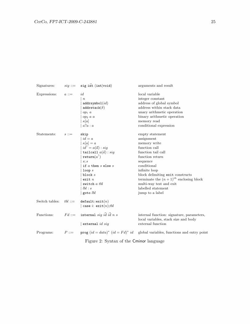
Cminor is a simple, low-level imperative language, comparable to a stripped-down, typelessvariant of C. Again we refer to the CompCert project for its formal definition and we just recallin figure 5.2 its syntax which as for Clight is structured in expressions, statements, functions,and whole programs.

Translation of Clight to Cminor. As in Cminor stack operations are made explicit, one hasto know which variables are stored in the stack. This information is produced by a staticanalysis that determines the variables whose address may be ‘taken’. Also space is reservedfor local arrays and structures. In a second step, the proper compilation is performed: itconsists mainly in translating Clight control structures to the basic ones available in Cminor.

5.3 RTLAbs

RTLAbs is the last architecture independent language in the compilation process. It is a ratherstraightforward abstraction of the architecture-dependent RTL intermediate language availablein the CompCert project and it is intended to factorize some work common to the varioustarget assembly languages (e.g. optimizations) and thus to make retargeting of the compilera simpler matter.

We stress that in RTLAbs the structure of Cminor expressions is lost and that this may havea negative impact on the following instruction selection step. Still, the subtleties of instructionselection seem rather orthogonal to our goals and we deem the possibility of retargeting easilythe compiler more important than the efficiency of the generated code.

CerCo, FP7-ICT-2009-C-243881 24

Expressions: a ::= id variable identifier| n integer constant| sizeof(τ) size of a type| op1 a unary arithmetic operation| a op2 a binary arithmetic operation| ∗a pointer dereferencing| a.id field access| &a taking the address of| (τ)a type cast| a?a : a conditional expression

Statements: s ::= skip empty statement| a = a assignment| a = a(a∗) function call| a(a∗) procedure call| s; s sequence| if a then s else s conditional| switch a sw multi-way branch| while a do s “while” loop| do s while a “do” loop| for(s,a,s) s “for” loop| break exit from current loop| continue next iteration of the current loop

| return a? return from current function| goto lbl branching| lbl : s labelled statement

Switch cases: sw ::= default : s default case| case n : s; sw labelled case

Variable declarations: dcl ::= (τ id)∗ type and name

Functions: Fd ::= τ id(dcl){dcl; s} internal function| extern τ id(dcl) external function

Programs: P ::= dcl;Fd∗; main = id global variables, functions, entry point

Figure 1: Syntax of the Clight language

CerCo, FP7-ICT-2009-C-243881 25

Signatures: sig ::= sig ~int (int|void) arguments and result

Expressions: a ::= id local variable| n integer constant| addrsymbol(id) address of global symbol| addrstack(δ) address within stack data| op1 a unary arithmetic operation| op2 a a binary arithmetic operation| κ[a] memory read| a?a : a conditional expression

Statements: s ::= skip empty statement| id = a assignment| κ[a] = a memory write

| id? = a(~a) : sig function call| tailcall a(~a) : sig function tail call

| return(a?) function return| s; s sequence| if a then s else s conditional| loop s infinite loop| block s block delimiting exit constructs

| exit n terminate the (n+ 1)th enclosing block| switch a tbl multi-way test and exit| lbl : s labelled statement| goto lbl jump to a label

Switch tables: tbl ::= default:exit(n)| case i: exit(n);tbl

Functions: Fd ::= internal sig ~id ~id n s internal function: signature, parameters,local variables, stack size and body

| external id sig external function

Programs: P ::= prog (id = data)∗ (id = Fd)∗ id global variables, functions and entry point

Figure 2: Syntax of the Cminor language

CerCo, FP7-ICT-2009-C-243881 26

return type ::= int || void signature ::= (int→)∗ return type

memq ::= int8s || int8u || int16s || int16u || int32 fun ref ::= fun name || psd reg

instruction ::= || skip→ node (no instruction)|| psd reg := op(psd reg∗)→ node (operation)|| psd reg := &var name → node (address of a global)|| psd reg := &locals[n]→ node (address of a local)|| psd reg := fun name → node (address of a function)|| psd reg := memq(psd reg [psd reg ])→ node (memory load)|| memq(psd reg [psd reg ]) := psd reg → node (memory store)|| psd reg := fun ref (psd reg∗) : signature → node (function call)|| fun ref (psd reg∗) : signature (function tail call)|| test op(psd reg∗)→ node,node (branch)|| return psd reg? (return)

fun def ::= fun name(psd reg∗) : signatureresult :psd reg?locals :psd reg∗

stack :nentry :nodeexit :node(node :instruction)∗

init datum ::= reserve(n) || int8(n) || int16(n) || int32(n) init data ::= init datum+

global decl ::= var var name{init data} fun decl ::= extern fun name(signature) || fun def

program ::= global decl∗

fun decl∗

Table 11: Syntax of the RTLAbs language

Syntax. In RTLAbs, programs are represented as control flow graphs (CFGs for short).We associate with the nodes of the graphs instructions reflecting the Cminor commands. Asusual, commands that change the control flow of the program (e.g. loops, conditionals) aretranslated by inserting suitable branching instructions in the CFG. The syntax of the languageis depicted in table 11. Local variables are now represented by pseudo registers that areavailable in unbounded number. The grammar rule op that is not detailed in table 11 definesusual arithmetic and boolean operations (+, xor, ≤, etc.) as well as constants and conversionsbetween sized integers.

Translation of Cminor to RTLAbs. Translating Cminor programs to RTLAbs programsmainly consists in transforming Cminor commands in CFGs. Most commands are sequen-tial and have a rather straightforward linear translation. A conditional is translated in abranch instruction; a loop is translated using a back edge in the CFG.

CerCo, FP7-ICT-2009-C-243881 27

size ::= Byte || HalfWord ||Word fun ref ::= fun name || psd reg

instruction ::= || skip→ node (no instruction)|| psd reg := n→ node (constant)|| psd reg := unop(psd reg)→ node (unary operation)|| psd reg := binop(psd reg , psd reg)→ node (binary operation)|| psd reg := &globals[n]→ node (address of a global)|| psd reg := &locals[n]→ node (address of a local)|| psd reg := fun name → node (address of a function)|| psd reg := size(psd reg [n])→ node (memory load)|| size(psd reg [n]) := psd reg → node (memory store)|| psd reg := fun ref (psd reg∗)→ node (function call)|| fun ref (psd reg∗) (function tail call)|| test uncon(psd reg)→ node,node (branch unary condition)|| test bincon(psd reg , psd reg)→ node,node (branch binary condition)|| return psd reg? (return)

fun def ::= fun name(psd reg∗) program ::= globals : nresult :psd reg? fun def ∗

locals :psd reg∗

stack :nentry :nodeexit :node(node :instruction)∗

Table 12: Syntax of the RTL language

5.4 RTL

As in RTLAbs, the structure of RTL programs is based on CFGs. RTL is the first architecture-dependant intermediate language of our compiler which, in its current version, targets theMips assembly language.

Syntax. RTL is very close to RTLAbs. It is based on CFGs and explicits the Mips instruc-tions corresponding to the RTLAbs instructions. Type information disappears: everything isrepresented using 32 bits integers. Moreover, each global of the program is associated to anoffset. The syntax of the language can be found in table 12. The grammar rules unop, binop,uncon, and bincon, respectively, represent the sets of unary operations, binary operations,unary conditions and binary conditions of the Mips language.

Translation of RTLAbs to RTL. This translation is mostly straightforward. A RTLAbsinstruction is often directly translated to a corresponding Mips instruction. There are a fewexceptions: some RTLAbs instructions are expanded in two or more Mips instructions. Whenthe translation of a RTLAbs instruction requires more than a few simple Mips instruction, itis translated into a call to a function defined in the preamble of the compilation result.

5.5 ERTL

As in RTL, the structure of ERTL programs is based on CFGs. ERTL explicits the callingconventions of the Mips assembly language.

CerCo, FP7-ICT-2009-C-243881 28

size ::= Byte || HalfWord ||Word fun ref ::= fun name || psd reg

instruction ::= || skip→ node (no instruction)|| NewFrame→ node (frame creation)|| DelFrame→ node (frame deletion)|| psd reg := stack[slot , n]→ node (stack load)|| stack[slot , n] := psd reg → node (stack store)|| hdw reg := psd reg → node (pseudo to hardware)|| psd reg := hdw reg → node (hardware to pseudo)|| psd reg := n→ node (constant)|| psd reg := unop(psd reg)→ node (unary operation)|| psd reg := binop(psd reg , psd reg)→ node (binary operation)|| psd reg := fun name → node (address of a function)|| psd reg := size(psd reg [n])→ node (memory load)|| size(psd reg [n]) := psd reg → node (memory store)|| fun ref (n)→ node (function call)|| fun ref (n) (function tail call)|| test uncon(psd reg)→ node,node (branch unary condition)|| test bincon(psd reg , psd reg)→ node,node (branch binary condition)|| return b (return)

fun def ::= fun name(n) program ::= globals : nlocals :psd reg∗ fun def ∗

stack :nentry :node(node :instruction)∗

Table 13: Syntax of the ERTL language

Syntax. The syntax of the language is given in table 13. The main difference between RTLand ERTL is the use of hardware registers. Parameters are passed in specific hardware registers;if there are too many parameters, the remaining are stored in the stack. Other conventionallyspecific hardware registers are used: a register that holds the result of a function, a registerthat holds the base address of the globals, a register that holds the address of the top of thestack, and some registers that need to be saved when entering a function and whose valuesare restored when leaving a function. Following these conventions, function calls do not listtheir parameters anymore; they only mention their number. Two new instructions appearto allocate and deallocate on the stack some space needed by a function to execute. Alongwith these two instructions come two instructions to fetch or assign a value in the parametersections of the stack; these instructions cannot yet be translated using regular load and storeinstructions because we do not know the final size of the stack area of each function. At last,the return instruction has a boolean argument that tells whether the result of the functionmay later be used or not (this is exploited for optimizations).

Translation of RTL to ERTL. The work consists in expliciting the conventions previouslymentioned. These conventions appear when entering, calling and leaving a function, and whenreferencing a global variable or the address of a local variable.

Optimizations. A liveness analysis is performed on ERTL to replace unused instructions bya skip. An instruction is tagged as unused when it performs an assignment on a register thatwill not be read afterwards. Also, the result of the liveness analysis is exploited by a register

CerCo, FP7-ICT-2009-C-243881 29

size ::= Byte || HalfWord ||Word fun ref ::= fun name || hdw reg

instruction ::= || skip→ node (no instruction)|| NewFrame→ node (frame creation)|| DelFrame→ node (frame deletion)|| hdw reg := n→ node (constant)|| hdw reg := unop(hdw reg)→ node (unary operation)|| hdw reg := binop(hdw reg , hdw reg)→ node (binary operation)|| hdw reg := fun name → node (address of a function)|| hdw reg := size(hdw reg [n])→ node (memory load)|| size(hdw reg [n]) := hdw reg → node (memory store)|| fun ref ()→ node (function call)|| fun ref () (function tail call)|| test uncon(hdw reg)→ node,node (branch unary condition)|| test bincon(hdw reg , hdw reg)→ node,node (branch binary condition)|| return (return)

fun def ::= fun name(n) program ::= globals : nlocals :n fun def ∗

stack :nentry :node(node :instruction)∗

Table 14: Syntax of the LTL language

allocation algorithm whose result is to efficiently associate a physical location (a hardwareregister or an address in the stack) to each pseudo register of the program.

5.6 LTL

As in ERTL, the structure of LTL programs is based on CFGs. Pseudo registers are not usedanymore; instead, they are replaced by physical locations (a hardware register or an addressin the stack).

Syntax. Except for a few exceptions, the instructions of the language are those of ERTLwith hardware registers replacing pseudo registers. Calling and returning conventions wereexplicited in ERTL; thus, function calls and returns do not need parameters in LTL. Thesyntax is defined in table 14.

Translation of ERTL to LTL. The translation relies on the results of the liveness analysisand of the register allocation. Unused instructions are eliminated and each pseudo register isreplaced by a physical location. In LTL, the size of the stack frame of a function is known;instructions intended to load or store values in the stack are translated using regular load andstore instructions.

Optimizations. A graph compression algorithm removes empty instructions generated byprevious compilation passes and by the liveness analysis.

CerCo, FP7-ICT-2009-C-243881 30

size ::= Byte || HalfWord ||Word fun ref ::= fun name || hdw reg

instruction ::= || NewFrame (frame creation)|| DelFrame (frame deletion)|| hdw reg := n (constant)|| hdw reg := unop(hdw reg) (unary operation)|| hdw reg := binop(hdw reg , hdw reg) (binary operation)|| hdw reg := fun name (address of a function)|| hdw reg := size(hdw reg [n]) (memory load)|| size(hdw reg [n]) := hdw reg (memory store)|| call fun ref (function call)|| tailcall fun ref (function tail call)|| uncon(hdw reg)→ node (branch unary condition)|| bincon(hdw reg , hdw reg)→ node (branch binary condition)|| mips label : (Mips label)|| goto mips label (goto)|| return (return)

fun def ::= fun name(n) program ::= globals : nlocals :n fun def ∗

instruction∗

Table 15: Syntax of the LIN language

5.7 LIN

In LIN, the structure of a program is no longer based on CFGs. Every function is representedas a sequence of instructions.

Syntax. The instructions of LIN are very close to those of LTL. Program labels, gotos andbranch instructions handle the changes in the control flow. The syntax of LIN programs isshown in table 15.

Translation of LTL to LIN. This translation amounts to transform in an efficient way thegraph structure of functions into a linear structure of sequential instructions.

5.8 Mips

Mips is a rather simple assembly language. As for other assembly languages, a program in Mipsis a sequence of instructions. The Mips code produced by the compilation of a Clight programstarts with a preamble in which some useful and non-primitive functions are predefined (e.g.conversion from 8 bits unsigned integers to 32 bits integers). The subset of the Mips assemblylanguage that the compilation produces is defined in table 16.

Translation of LIN to Mips. This final translation is simple enough. Stack allocation anddeallocation are explicited and the function definitions are sequentialized.

CerCo, FP7-ICT-2009-C-243881 31

load ::= lb || lhw || lw store ::= sb || shw || sw fun ref ::= fun name || hdw reg

instruction ::= || nop (empty instruction)|| li hdw reg , n (constant)|| unop hdw reg , hdw reg (unary operation)|| binop hdw reg , hdw reg , hdw reg (binary operation)|| la hdw reg , fun name (address of a function)|| load hdw reg , n(hdw reg) (memory load)|| store hdw reg , n(hdw reg) (memory store)|| call fun ref (function call)|| uncon hdw reg ,node (branch unary condition)|| bincon hdw reg , hdw reg ,node (branch binary condition)|| mips label : (Mips label)|| j mips label (goto)|| return (return)

program ::= globals : nentry : mips label∗

instruction∗

Table 16: Syntax of the Mips language

1. Label the input Clight program.

2. Compile the labelled Clight program in the labelled world. This produces a labelled Mips code.

3. For each label of the labelled Mips code, compute the cost of the instructions under its scope and generatea label-cost mapping. An unlabelled Mips code — the result of the compilation — is obtained by removing thelabels from the labelled Mips code.

4. Add a fresh cost variable to the labelled Clight program and replace the labels by an increment of this cost

variable according to the label-cost mapping. The result is an annotated Clight program with no label.

Table 17: Building the annotation of a Clight program in the labelling approach

6 Labelling approach for the C compiler

This section informally describes the labelled extensions of the languages in the compilationchain, the way the labels are propagated by the compilation functions, the labelling of thesource code, the hypotheses on the control flow of the labelled Mips code and the verificationthat we perform on it, the way we build the instrumentation, and finally the way the labellingapproach has been tested. The process of annotating a Clight program using the labellingapproach is summarized in table 17 and is detailed in the following sections.

6.1 Labelled Clight and labelled Cminor

Both the Clight and Cminor languages are extended in the same way by labelling both state-ments and expressions (by comparison, in the toy language Imp we just labelled statementsand boolean conditions). The labelling of expressions aims to capture precisely their executioncost. Indeed, Clight and Cminor include expressions such as a1?a2; a3 whose evaluation costdepends on the boolean value a1.

As both languages are extended in the same way, the extended compilation does nothing

CerCo, FP7-ICT-2009-C-243881 32

more than sending Clight labelled statements and expressions to Cminor labelled statementsand expressions.

6.2 Labels in RTLAbs and the back-end languages

The labelled version of RTLAbs and the languages in the back-end language simply consistsin adding a new instruction whose semantics is to emit a label without modifying the state.For the CFG based languages (RTLAbs to LTL), this new instruction is emit label → node.For LIN and Mips, it is emit label . The translation of these label instructions is immediate. InMips, we also rely on a reserved label begin function to pinpoint the beginning of a functioncode (cf. section 6.3.6).

6.3 Labelling of the source language

The goal here is to add labels in the source program that cover every reachable instruction ofthe program and avoid unlabelled loops; this can be seen as a soundness property. Anotherimportant point is precision, meaning that a label might cover several paths to the nextlabels only if those paths have equal costs. Several labellings might satisfy the soundness andprecision conditions, but from an engineering point of view, a labelling that makes obviouswhich instruction is under the scope of which label would be better. There is a thin line tofind between too many labels — which may obfuscate the code — and too few labels — whichmakes it harder to see which instruction is under the scope of which label. The balance leansa bit towards the economy of labels because the cost of executing an assembly instructionoften depends on its context (for instance by the status of the cache memory). We explainour labelling by considering the constructions of Clight and their compilation to Mips.

6.3.1 Sequential instructions

A sequence of Clight instructions that compile to sequential Mips code, such as a sequence ofassignments, can be handled by a single label which covers the unique execution path. Theexample below illustrates the labelling of ‘sequential’ Clight instructions.

ClightLabelling−−−−−−→ Labelled Clight

Compilation−−−−−−−−→ Labelled Mips

i = 0; cost: emit costtab[i] = x; i = 0; li $v0, 4

x++; tab[i] = x; mul $v0, $zero, $v0

x++; add $v0, $a1, $v0

sw $a0, 0($v0)

li $v0, 1

add $a0, $a0, $v0

6.3.2 Ternary expressions

Most Clight expressions compile to sequential Mips code. There is one exception: ternaryexpressions that introduce a branching in the control flow. Because of the precision condition,we must associate a label with each branch.

CerCo, FP7-ICT-2009-C-243881 33

ClightLabelling−−−−−−→ Labelled Clight

Compilation−−−−−−−−→ Labelled Mips

b ? x+1 : b ? ( cost1: x+1) : beq $a0, $zero, c false

y ( cost2: y) emit cost1li $v0, 1

add $v0, $a1, $v0

j exit

c false:

emit cost2move $v0, $a2

exit:

Related cases. The two Clight boolean operations && and || have a lazy semantics: de-pending on the evaluation of the first argument, the second one might be evaluated or not.There is an obvious translation to ternary expressions. For instance, the expression x && y

is translated into the expression x?(y?1:0):0. Our compiler performs this translation beforecomputing the labelling.

6.3.3 Conditionals

Conditionals are another way to introduce a branching. As for ternary expressions, the la-belling of a conditional consists in adding a starting label to the labelling of each branch.

ClightLabelling−−−−−−→ Labelled Clight

Compilation−−−−−−−−→ Labelled Mips

if (b) { if (b) { beq $a0, $zero, c false

x = 1; cost1: emit cost1... } x = 1; li $v0, 1

else { ... } ...

x = 2; else { j exit

... } cost2: c false:

x = 2; emit cost2... } li $v0, 2

...

exit:

6.3.4 Loops

Loops in Clight are guarded by a condition. Following the arguments of the previous cases,we add two labels when encountering a loop construct: one label to start the loop’s body, andone label when exiting the loop. This is enough to guarantee that the loop in the compiledcode goes through a label.

ClightLabelling−−−−−−→ Labelled Clight

Compilation−−−−−−−−→ Labelled Mips

while (b) { while (b) { loop:

i++; cost1: beq $a0, $zero, exit

... } i++; emit cost1x = i; ... } li $v0, 1

cost2: add $a1, $a1, $v0

x = i; ...

j loop

exit:

emit cost2move $a2, $a1

CerCo, FP7-ICT-2009-C-243881 34

6.3.5 Program Labels and Gotos

In Clight, program labels and gotos are intraprocedural. Their only effect on the control flowof the resulting assembly code is to potentially introduce an unguarded loop. This loop mustcontain at least one cost label in order to satisfy the soundness condition, which we ensure byadding a cost label right after a program label.

ClightLabelling−−−−−−→ Labelled Clight

Compilation−−−−−−−−→ Labelled Mips

lbl: lbl: lbl:

i++; cost: emit cost... i++; li $v0, 1

goto lbl; ... add $a0, $a0, $v0

goto lbl; ...

j lbl

6.3.6 Function calls

Function calls in Mips are performed by indirect jumps, the address of the callee being ina register. In the general case, this address cannot be inferred statically. Even though thedestination point of a function call is unknown, when the considered Mips code has beenproduced by our compiler, we know for a fact that this function ends with a return statementthat transfers the control back to the instruction following the function call in the caller. Asa result, we treat function calls according to the following principles: (1) the instructions ofa function are covered by the labels inside this function, (2) we assume a function call alwaysreturns and runs the instruction following the call.

Principle (1) entails in particular that each function must contain at least one label. Toensure this, we simply add a starting label in every function definition. The example belowillustrates this point:

ClightLabelling−−−−−−→ Labelled Clight

Compilation−−−−−−−−→ Labelled Mips

void f () { void f () { f start:

f’s body cost: Frame Creation} f’s body Initializations

} emit costf’s bodyFrame Deletionreturn

We notice that some instructions in Mips will be inserted before the first label is emit-ted. These instructions relate to the frame creation and/or variable initializations, and arecomposed of sequential instructions (no branching). To deal with this issue, we take the con-vention that the instructions that precede the first label in a function code are actually underthe scope of the first label.

Principle (2) is of course an over-approximation of the program behaviour as a functionmight fail to return because of an infinite loop. In this case, the proposed labelling remainscorrect: it just assumes that the instructions following the function call will be executed, andtakes their cost into consideration. The final computed cost is still an over-approximation ofthe actual cost.

CerCo, FP7-ICT-2009-C-243881 35

6.4 Verifications on the object code

The labelling previously described has been designed so that the compiled Mips code satisfiesthe soundness and precision conditions. However, we do not need to prove this, instead wehave to devise an algorithm that checks the conditions on the compiled code. The algorithmassumes a correct management of function calls in the compiled code. In particular, whenwe call a function we always jump to the first instruction of the corresponding code segmentand when we return we always jump to an an instruction that follows a call. We stress thatthis is a reasonable hypothesis that is essentially subsumed by the proof that the object codesimulates the source code.

In our current implementation, we check the soundness and the precision conditions whilebuilding at the same time the label-cost mapping. To this end, the algorithm takes thefollowing main steps.

• First, for each function a control flow graph is built.

• For each graph, we check whether there is a unique label that is reachable from the rootby a unique path. This unique path corresponds to the instructions generated by thecalling conventions as discussed in section 6.3.6. We shift the occurrence of the label tothe root of the graph.

• By a strongly connected components algorithm, we check whether every loop in thegraphs goes through at least one label.

• We perform a (depth-first) search of the graph. Whenever we reach a labelled node,we perform a second (depth-first) search that stops at labelled nodes and computes anupper on the cost of the occurrence of the label. Of course, when crossing a branchinginstruction, we take the maximum cost of the branches. When the second search stopswe update the current cost of the label-cost mapping (by taking a maximum) and wecontinue the first search.

• Warning messages are emitted whenever the maximum is taken between two differentvalues as in this case the precision condition may be violated.

6.5 Building the cost annotation

Once the label-cost mapping is computed, instrumenting the labelled source code is an easytask. A fresh global variable which we call cost variable is added to the source program withthe purpose of holding the cost value and it is initialised at the very beginning of the main

program. Then, every label is replaced by an increment of the cost variable according to thelabel-cost mapping. Following this replacement, the cost labels disappear and the result is aClight program with annotations in the form of assignments.

There is one final problem: labels inside expressions. As we already mentioned, Clight doesnot allow writing side-effect instructions — such as cost increments — inside expressions. Tocope with this restriction, we produce first an instrumented C program — with side-effects inexpressions — that we translate back to Clight using CIL. This process is summarized below.

Labelled Clightlabel-cost mapping

}Instrumentation−−−−−−−−−−→ Instrumented C

CIL−−→ Instrumented Clight

CerCo, FP7-ICT-2009-C-243881 36

6.6 Testing

It is desirable to test the coherence of the labelling from Clight to Mips. To this end, eachlabelled language comes with an interpreter that produces the trace of the labels encounteredduring the computation. Then, one naive approach is to test the equality of the traces pro-duced by the program at the different stages of the compilation. Our current implementationpasses this kind of tests. For some optimisations that may re-order computations, a weakercondition could be considered which consists in abstracting the traces as multi-sets of labelsbefore comparing them.

7 Conclusion and future work

We have discussed the problem of building a compiler which can lift in a provably correctway pieces of information on the execution cost of the object code to cost annotations on thesource code. To this end, we have introduced the so called direct and labelling approaches anddiscussed their formal application to a toy compiler. Based on this experience, we have arguedthat the second approach has better scalability properties. To substantiate this claim, we havereported on our successful experience in implementing and testing the labelling approach ontop of a prototype compiler written in ocaml for a large fragment of the C language which canbe shortly described as Clight without floating point.

We discuss next a few directions for future work. First, we plan to test the current compileron the kind of C code produced for embedded applications, a typical example being the C codeproduced by the compilation of synchronous languages such as Lustre or Esterel. Starting fromthe annotated C code, we expect to produce automatically meaningful information on, say, thereaction time of a given synchronous program. Second, we plan to port the current compilerto commercial assembly languages. In particular, it would be interesting to target one of theassembly languages covered by the AbsInt tool so as to obtain more realistic estimations of theexecution cost of sequences of instructions. Third, we plan to formalise and validate in theCalculus of Inductive Constructions the prototype implementation of the labelling approachfor the C compiler described in section 5. This requires a major implementation effort whichwill be carried on in collaboration with our partners of the CerCo project [2]. Fourth, weplan to study the applicability of the labelling approach to other optimisation techniques inthe realm of the C compilers technology such as loop optimisations, and to other languageswhich rely on rather distinct compilation technologies such as a language of the ML family.

References

[1] AbsInt Angewandte Informatik. http://www.absint.com/.

[2] Certified Complexity (Project description). ICT-2007.8.0 FET Open, Grant 243881.http://cerco.cs.unibo.it.

[3] Esterel Technologies. http://www.esterel-technologies.com.

[4] Frama− C software analysers. http://frama-c.com/.

[5] C. Ferdinand, R. Heckmann, T. Le Sergent, D. Lopes, B. Martin, X. Fornari, and F. Martin. Combininga high-level design tool for safety-critical systems with a tool for WCET analysis of executables. In Proc.of the 4th European Congress on Embedded Real Time Software (ERTS), Toulouse, 2008.

[6] X. Fornari. Understanding how SCADE suite KCG generates safe C code. White paper, Esterel Tech-nologies, 2010.

CerCo, FP7-ICT-2009-C-243881 37

[7] J. Larus. Assemblers, linkers, and the SPIM simulator. Appendix of Computer Organization and Design:the hardware/software interface, book by Hennessy and Patterson, 2005.

[8] X. Leroy. Formal verification of a realistic compiler. Commun. ACM, 52(7):107-115, 2009.

[9] X. Leroy. Mechanized semantics, with applications to program proof and compiler verification (lecturenotes and Coq development). Marktoberdorf summer school, Germany, 2009.

[10] J. McCarthy and J. Painter. Correctness of a compiler for arithmetic expressions. In Mathematical aspectsof computer science 1, volume 19 of Symposia in Applied Mathematics, AMS, 1967.

[11] G. Necula, S. McPeak, S.P. Rahul, and W. Weimer. CIL: Intermediate Language and Tools for Analysisand Transformation of C Programs. In Proceedings of Conference on Compiler Construction, SpringerLNCS 2304:213–228, 2002.

[12] F. Pottier. Compilation (INF 564), Ecole Polytechnique, 2009-2010.http://www.enseignement.polytechnique.fr/informatique/INF564/.

[13] R. Wilhelm et al. The worst-case execution-time problem - overview of methods and survey of tools. ACMTrans. Embedded Comput. Syst., 7(3), 2008.

CerCo, FP7-ICT-2009-C-243881 38

A Proofs

A.1 Notation

Lett−→ be a family of reduction relations where t ranges over the set of labels and ε. Then we

define:

t⇒=

{(ε−→)∗ if t = ε

(ε−→)∗◦ t−→ ◦( ε−→)∗ otherwise

where as usual R∗ denote the reflexive and transitive closure of the relation R and ◦ denotesthe composition of relations.

A.2 Proof of proposition 4

The following properties are useful.

Lemma 26 (1) The relationC; is transitive.

(2) If iC; j and R(C, j,K) then R(C, i,K).

The first property can be proven by induction on the definition ofC; and the second by

induction on the structure of K. Next we can focus on the proposition. The notation Ci· C ′

means that i = |C|. Suppose that:

(S,K, s)→ (S′,K′, s′) (1) and R(C, i, S ·K) (2) .

From (2), we know that there exist i′ and i′′ such that:

iC; i′ (3), C = C1

i′· C(S)i′′· C2 (4), and R(C, i′′,K) (5)

and from (3) it follows that:

C ` (i, σ, s)∗→ (i′, σ, s) (3′) .

We are looking for j such that:

C ` (i, σ, s)∗→ (j, σ, s′) (6), and R(C, j, S′ ·K′) (7) .

We proceed by case analysis on S. We just detail the case of the conditional command as thethe remaining cases have similar proofs. If S = if e1 < e2 then S1 else S2 then (4) is rewrittenas follows:

C = C1i′· C(e1) · C(e2).bge(k1)

a· C(S1)b· branch(k2)

c· C(S2)i′′· C2

where c = a + k1 and i′′ = c + k2. We distinguish two cases according to the evaluation ofthe boolean condition. We describe the case (e1 < e2) ⇓ true. We set j = a.

• The instance of (1) is (S,K, s)→ (S1,K, s).

• The reduction required in (6) takes the form C ` (i, σ, s)∗→ (i′, σ, s)

∗→ (a, σ, s′), and itfollows from (3′), the fact that (e1 < e2) ⇓ true, and proposition 3(2).

• Property (7), follows from lemma 26(2), fact (5), and the following proof tree:

jC; j b

C; i′′ R(C, i′′,K)

R(C, b,K)

R(C, j, S1 ·K)

.

2

CerCo, FP7-ICT-2009-C-243881 39

A.3 Proof of proposition 8

We recall that the compiled code C′(C) does not read or write the locations lcost , lA, and lB.Then we note the following properties.

(a) If AnVm(C) ` (5 · i, σ, s)→5 (5 · j, σ′, s′) then C ` (i, σ, s)→ (j, σ′, s′[s(cost)/cost ]).

(b) If M ` (i,m)→ (j,m′) then AnMips(M) ` (9 · i,m)∗→ (9 · j,m′[m(lcost) + 1/lcost ,m(A)/lA,m(B)/lB ]).

Using (a) and the hypothesis, we derive:

C ` (i, σ, s)→ (j, σ′, s′[s(cost)/cost ])

Then, by proposition 6 and the hypothesis on m we derive:

C′(C) ` (p(i, C),m)∗→ (p(j, C),m′) and m′ ‖−σ′, s′[s(cost)/cost ] (7)

We perform a case analysis on the instruction C[i] and h(i) to derive:

AnMips(C′(C)) ` (9 · p(i, C),m)∗→ (9 · p(j, C),m′[m(lcost) + d(i, C)/lcost , x/lA, y/lB ])

where x and y are respectively the value of lA and lB in the last intermediate configuration.

The memory realisation. The final memory state is: m′[m(lcost)+d(i, C)/lcost , x/lA, y/lB].Then we have to verify:

(m′[m(lcost) + d(i, C)/lcost , x/lA, y/lB ])[s′(cost)/lcost ] ‖−σ′, s′ .

This is equivalent to:

m′[s′(cost)/lcost , x/lA, y/lB ] ‖−σ′, s′ .

Since the realisation predicate does not depend on the locations lA and lB, we can concludeusing the second part of (7).

The inequation. To conclude, we verify the inequation:

m′[m(lcost) + d(i, C)/lcost , x/lA, y/lB ](lcost)−m(lcost) ≤ s′(cost)− s(cost) .

By rewriting, we get: d(i, C) ≤ s′(cost) − s(cost). This follows by case analysis of C[i] andh(i) since, by definition, AnVm uses the worst possible value of d(i, C). 2

A.4 Proof of proposition 10

We have P = prog S and by definition, An Imp(P ) = cost := cost + κ(S); An Imp(S). Withour simulation hypothesis, we derive (An Imp(S), s[κ(S)/cost ]) ⇓ s′[c′/cost ]. Using the propo-sition 9 with C = C ′ = ε, d = 0 and σ = ε, we have:

AnVm(C(S)) ` (0, ε, s[0/cost ])∗→ (|AnVm(C(P ))|, ε, s′[d′/cost ]) ,

where d′ ≤ (c′ − κ(S)) + κ(S) = c′. By definition, C(P ) = C(S) · halt and |AnVm(C(P ))| =5 · |C(P )|. We can rewrite the simulation:

AnVm(C(P )) ` (0, ε, s[0/cost ])∗→ (5 · |C(P )|, ε, s′[d′/cost ]) .

By proposition 5, there is a decoration h such that C(P ) : h and h(0) = 0. By iteratingproposition 8, we derive:

AnMips(C′(C(P ))) ` (9 · p(0, C(P )),m)∗→ (9 · p(|C(P )|, C(P )),m′) ,

CerCo, FP7-ICT-2009-C-243881 40

withm′[d′/lcost ] ‖−ε, s′[d′/cost ] andm′(lcost) ≤ d′. We know that the last instruction of C(P ) isan halt, therefore the last instruction of C′(C(P )) is also an halt. By definition, p(|C(P )|, C(P ))is the position after this instruction. That gives us:

(AnMips(C′(C(P ))),m) ⇓ m′ .

And by transitivity we have: m′(lcost) ≤ d′ ≤ c′. 2

A.5 Proof of proposition 11

(1) By induction on the structure of the command S.

(2) By iterating the following proposition.

Proposition 27 If (S,K, s)t→ (S′,K ′, s′) and R(C, i, S · K) with t = ` or t = ε then C `

(i, σ, s)t⇒ (j, σ, s′) and R(C, j, S′ ·K ′).

This is an extension of proposition 4 and it is proven in the same way with an additionalcase for labelled commands. 2

A.6 Proof of proposition 13

(1) The compilation of the Vm instruction nop(`) is the Mips instruction (nop `).

(2) By iterating the following proposition.

Proposition 28 Let C : h be a well formed code. If C ` (i, σ, s)t→ (j, σ′, s′) with t = ` or

t = ε, h(i) = |σ| and m ‖−σ, s then C′(C) ` (p(i, C),m)t⇒ (p(j, C),m′) and m′ ‖−σ′, s′.

This is an extension of proposition 6 and it is proven in the same way with an additionalcase for the nop instruction. 2

A.7 Proof of proposition 14

In order to carry on the proof, one needs to develop a bit more the properties of the small-stepoperational semantics. In particular, one needs to show that a continuation such as S · (S′ ·K)is ‘observationally equivalent’ to the continuation (S;S′) ·K. 2

A.8 Proof of proposition 16

By diagram chasing using propositions 11(1), 13(1), and the definition 15 of labelling. 2

A.9 Proof of proposition 17

Suppose that:(I(L(P )), s[c/cost ]) ⇓ s′[c+ δ/cost ] and m ‖−s[c/cost ] .

Then, by proposition 14, for some λ:

(L(P ), s[c/cost ]) ⇓ (s′[c/cost ], λ) and κ(λ) = δ .

Finally, by propositions 11(2) and 13(2) :

(C′(C(L(P ))),m) ⇓ (m′, λ) and m′ ‖−s′[c/cost ] .

2

CerCo, FP7-ICT-2009-C-243881 41

A.10 Proof of proposition 20

If λ = `1 · · · `n then the computation is the concatenation of simple paths labelled with`1, . . . , `n. Since κ(`i) bounds the cost of a simple path labelled with `i, the cost of theoverall computation is bounded by κ(λ) = κ(`1) + · · ·κ(`n). 2

A.11 Proof of proposition 22

Same proof as proposition 20, by replacing the word bounds by is exactly and the wordsbounded by by exactly. 2

A.12 Proof of proposition 23

In both labellings under consideration the root node is labelled. An obvious observation is thatonly commands of the shape while b do S and while lb do S introduce loops in the compiledcode. In the second case, the compilation ensures that a label is placed in the loop. In the firstcase, we notice that both labelling introduce a label in the loop (though at different places).Thus all loops go through a label and the compiled code is always sound.

To show the precision of the second labelling Lp, we note the following property.

Lemma 29 A soundly labelled graph is precise if each label occurs at most once in the graphand if the immediate successors of the bge nodes are either halt (no successor) or labellednodes.

Indeed, in a such a graph starting from a labelled node we can follow a unique path upto a leaf, another labelled node, or a bge node. In the last case, the hypotheses in the lemma29 guarantee that the two simple paths one can follow from the bge node have the samelength/cost. 2

A.13 Proof of proposition 25

By applying consecutively proposition 17 and propositions 20 or 22. 2