informal export barriers and poverty - world...
TRANSCRIPT
Informal Export Barriers and Poverty∗
Guido G. Porto†
Development Research GroupThe World Bank
Abstract
This paper investigates the poverty impacts of informal export barriers like transportcosts, cumbersome customs practices, costly regulations, and bribes. I model theseinformal barriers as export taxes that distort the efficient allocation of resources.In low-income agricultural economies, this distortion lowers wages and householdagricultural income, thereby leading to higher poverty. In this paper, I investigatethe poverty impacts of improving export procedures in Moldova. This is a unique casestudy: poverty is widespread (half of the Moldovan population lives in poverty), thecountry is very open and relies on agricultural exports for growth, formal trade barriersare fairly liberalized, and informal export barriers are common and widespread. I findthat improving export practices would benefit the average Moldovan household acrossthe whole income distribution. For example, halving informal export barriers wouldcause poverty to decline from 48.3 percent of the population to between 43.3 and 45.5percent. This is a nontrivial effect that involves lifting 100,000-180,000 individuals outof poverty.
JEL CODES: F14-F16-I32-J43Key words: Informal trade barriers, trade costs, poverty
∗I am indebted to L. Bouton and P. Brenton for comments on earlier drafts and for putting together theWorld Bank Exporter and Importer Survey used in this paper. The Department of Statistics and Sociologyof the Republic of Moldova kindly allowed me to use the MBHS household dataset. I wish to thank I.Brambilla, H. Kee, A. Nicita and M. Olarreaga. The comments and suggestions of two anonymous refereesare greatly appreciated. All remaining errors and omissions are my responsibility.
†Correspondence: Guido Porto, MailStop MC3-303, The World Bank, 1818 H Street, Washington DC20433. email: [email protected]

1 Introduction
This paper provides novel evidence on the relationship between trade and poverty. Most of
the current literature explores the effects of formal trade liberalization on poverty or on the
distribution of income. For instance, Attanasio, Goldberg and Pavcnik (2004) investigate
the inequality impacts of trade reforms in Colombia, Friedman and Levinsohn (2002) study
the consequences of the financial crisis on the poor in Indonesia, and Porto (2003) studies
the distributional effects of Mercosur in Argentina. A recent literature looks instead at the
effects of trade on non-monetary outcomes: Edmonds and Pavcnik (2004a) study the impact
of export liberalization of rice on child labor in Vietnam, Goldberg and Pavcnik (2003)
explore the impacts of trade on informal labor markets, and Edmonds and Pavcnik (2004b)
study the impacts of trade liberalization on labor supply.
The present paper contributes to this literature by investigating a previously unexplored
aspect of international trade: the effects of informal export barriers on poverty. Informal
export barriers include transport costs, cumbersome customs practices, bureaucracy,
regulations, and corruption. These barriers are relevant because they hinder trade, and
the benefits that come with it, when formal trade liberalization has already been achieved.
In present days, as tariffs and non-tariff barriers are being eliminated, trade facilitation
practices are becoming increasingly more important. This paper is an attempt to look at
their poverty impacts in low-income countries.1
To investigate these issues, I have chosen to look at the Moldovan experience. This
is a unique case study. First, poverty is a serious concern in Moldova, where almost half
of the population lived in poverty in 2002. Second, Moldova is very open to trade with
low formal trade barriers. Instead, the level of informal barriers to trade and the costs
of doing business are quite high.2 Third, and more importantly, a brand new dataset
that can be used to measure the costs imposed by informal export barriers has recently
1There is a growing interest in informal trade costs; see the forthcoming survey by Anderson and vanWincoop (2003). The effects on poverty, however, have not received much attention yet.
2There are several reports that establish this fact. See, for instance, Ministry of Economy of the Republicof Moldova (2003), which assesses regulatory costs in Moldova. Section 2 describes these costs in moredetails.
1
become available. This is the World Bank Exporter and Importer Survey (EIS), a survey
especially prepared to quantify trade costs in Moldova. Trading firms provided information
on different impediments to import and export activities, including transport costs, unofficial
fees, regulatory costs, transaction costs, bribes, and others.
The methodology used in the paper links trade barriers to price changes and price changes
to poverty impacts. As a first step, I identify the price changes that would be brought
about by the (hypothetical) removal of informal export barriers. To do this, I model these
barriers as transaction costs or export taxes that distort the efficient allocation of resources
by reducing the net price received by exporters. Thus, improvements in export procedures
would raise domestic prices. I use the EIS data to quantify these trade costs. In Moldova, I
find that trade costs are equivalent to 24.5 percent of the value of an average shipment.
To link price changes with poverty changes, I proceed as follows. Agriculture processing
comprises the main Moldovan exports. The majority of the population works on the
fields, providing agricultural inputs to manufacturing firms, or in agro and food processing
industries. Consequently, I assume that households supply non-tradable inputs, such as labor
and agricultural inputs, to the exporting firms. An increase in the net price of exportable
goods raises the demand for the factors of production intensively used in agriculture,
particularly labor and agricultural inputs. As a result, wages and agro-input prices increase,
household income increases, and some households leave poverty. At the same time, the
increase in export prices raises the price of some food items, causing real income to decline
and poverty to increase. In the end, the net poverty impacts of the removal of export barriers
depend on whether the income effects dominate these latter consumption effects.
To measure these effects, I use the Moldovan Household Budget Survey (MHBS) - a
comprehensive household dataset - together with information on export prices. These data
are used to estimate the elasticities that measure the responses of labor income and household
agricultural income to changes in agro-manufacturing export prices. These elasticities are
combined with estimates of the price changes induced by the removal of trade barriers
to quantify the income effects. Similarly, the MHBS survey collects information on food
expenditures that I combine with the estimated price changes to quantify the consumption
2

effects. Finally, I merge the income effects and the consumption effects to predict the
(hypothetical) income that would be enjoyed by each Moldovan household if trade barriers
were reduced. Poverty impacts are assessed by computing and comparing the associated
head count ratios.
These are the main findings. Following a raise in the net price of agro-exports, I estimate
that both the price of agro-consumption goods and labor income increase. In contrast,
household agricultural income is not significantly affected. In the end, I find that the average
real income of Moldovan families increases for both the poor and the non-poor. For example,
higher export prices brought about by halving export barriers would cause household welfare
to increase by 4 to 8 percent (of initial expenditure) at the bottom of the distribution, by
3 to 5.5 percent for households at the poverty line, and by 5 to 11 percent at the upper
tail of the distribution. Poverty would decline from an initial head count ratio of 48.3
percent to a poverty rate of between 45.5 and 43.3 percent. This means that informal export
barriers would be responsible for lifting between 100,000 and 180,000 Moldovan citizens out
of poverty. With a total population of 3.5 million, these are large effects.
The paper is organized as follows. In section 2, I begin by describing the data on
informal barriers taken from the Exporter and Importer Survey. Section 3 develops a general
equilibrium trade model of the Moldovan economy that describes the theoretical connection
between informal export barriers, household income and poverty. In Section 4, I estimate
the responses of wages and agricultural income to changes in the prices faced by exporting
firms. In section 5, the poverty implications of the removal of some of the informal trade
barriers are assessed. Finally, Section 6 summarizes results and concludes.
2 Informal Barriers
In this paper, I focus on the role of informal barriers to trade on poverty alleviation.
The emphasis on informal barriers rather than on formal barriers reflects the fact that,
in Moldova, while formal trade has been already liberalized, informal barriers remain high
and impose large costs on producers. In 2002, for example, the average tariff was 5.2 percent;
3
tariff rates were arranged in bands, from a minimum of 0 percent to a maximum of only
25 percent. In addition, Moldova is a member of free trade areas with former Soviet Union
countries and Romania and thus those tariffs were applied on only 40 percent of all imports.
No formal trade restrictions were imposed on exports. On the contrary, as shown in this
section, the costs of doing business are much higher, around 25 percent on average.3
The Moldovan case provides a unique opportunity to quantify the costs of informal export
barriers because of the availability of a recent survey that gathered data on the cost of doing
business. This is the World Bank Exporter and Importer Survey (World Bank, 2003). The
EIS survey was designed to collect data to carry out a World Bank trade facilitation study in
Moldova. As opposed to previous reports on the cost of doing business (such as the Ministry
of Economy of the Republic of Moldova, 2003), the EIS survey collects, and reports, data at
the firm level. This allows for the quantification of trade costs.
A sample of 161 Moldovan trading enterprises was surveyed with the aim of assessing
external and internal constraints to trade. The sample covered both importers and exporters
across the country: 86 firms (53.4 percent) were exclusively importers, 18 firms (11.2 percent)
were exclusively exporters, and the remaining 57 firms (35.4 percent) were involved in exports
and imports simultaneously. Notice, however, that only 44.1 percent of the firms actually
exported in 2002. Of these exporting firms, 35.2 percent were in agro-manufacturing, 28.2
percent in manufacturing, and 32.4 percent in wholesale/retail trade.
Apart from general firm information, such as type of firms, form of ownership (private,
joint venture), main product line, and sales, specific questions regarding impediments to
trade were asked. These questions were organized around the following topics: A. Customs
and Tax Administration; B. Transportation, Shipping and Distribution; C. Testing and
Conformity Assessment; D. Export and Import Financing; E. Export Barriers; F. Duty
Preferences in Overseas Markets; G. Import Barriers. In this paper, I focus on items B and
E.
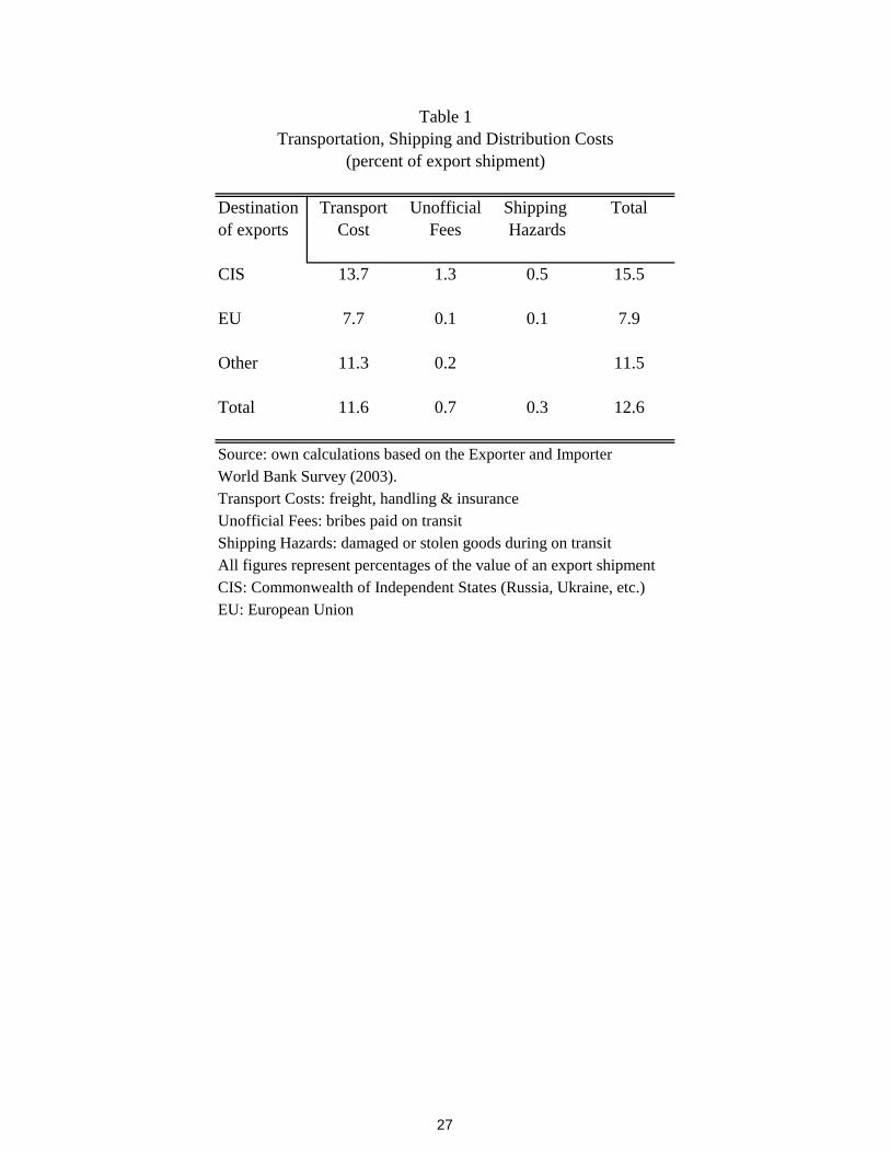
I begin by discussing the Transportation and Distribution (T&D) costs, reported in
Table 1. The data allow me to identify the source of the costs into different components:
3See the Ministry of Economy of the Republic of Moldova (2003) and World Bank (2003).
4

transport (freight, handling and insurance), unofficial fees, and shipping hazards (damaged
or stolen goods during shipping). I can also separate the costs by markets: Commonwealth
of Independent States (CIS, which includes former Soviet Union Republics), European Union
(EU), and Other markets. The total average Transportation & Distribution (T&D) costs
reach 12.6 percent of the value of a shipment. T&D costs to CIS countries (mainly Russia)
are 15.5 percent, to the EU, 7.9 percent and to other destinations, 11.5 percent. Most of
these costs are associated with transportation costs, which are, on average, equal to 11.6
percent. Unofficial fees amount to 0.7 percent and Shipping Hazards to 0.3 percent.
Being a landlocked country, bordered by Romania on the west and Ukraine on the
east, Moldova is trapped by its neighbors. Furthermore, corruption, bribes, and formal
and informal regulations are endemic to the region. On top of all this, organized crime
is prevalent in present-day CIS countries. These facts impose large trade costs that are,
in principle, differentiated by the destination of Moldovan exports. In Table 1, I report
that unofficial fees and shipping hazards costs are much higher for exports destined to CIS
countries than to the EU (or other destinations). For example, Unofficial Fees paid while
exporting to CIS are 1.3 percent, compared to a low 0.1 percent when exporting to the EU.
Similarly, the cost of damaged or stolen goods on transit to CIS countries is 5 times higher
than to Europe. This highlights the trade barriers associated with corruption and crime
when dealing with CIS partners.
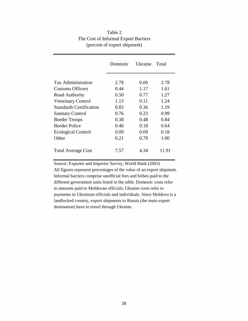
The costs associated with several additional barriers are reported in Table 2. These
informal export barriers include official (fees, fines) and unofficial (bribes) payments paid to
border police, border troops, sanitary controls, veterinary controls, standards certification,
customs officers, ecological controls, tax administration, and road authority. An important
fraction of these costs is imposed by Moldova’s internal regulations and corruption. But the
problems faced by exporters do not end when crossing the frontier or leaving customs. Quite
the contrary, Moldovan shipments with final destination in Russia and other CIS partners
often have to cross Ukraine, where they face important additional unofficial barriers. The
Exporter and Importer Survey allows me to separate the costs of the export barriers arising
from domestic sources from those arising from Ukrainian sources. These are in Table 2, too.
5
On average, the total cost of export barriers is equivalent to 11.9 percent of the value of a
shipment. Out of this total, 7.57 percentage points (a 63.5 percent of the total cost) originate
in Moldova while the remaining 4.33 percentage points (36.5 percent) are caused by the
Ukrainian neighbors. Tax Administration costs reach 2.78 percent, all of it inside Moldova.
Customs Officers absorb 1.61 percent; interestingly, payments to Ukrainian customs amount
to 1.17 percent, almost three times as large as the 0.44 percent of domestic costs. Road
Authority (1.27 percent; notice again the relative importance of Ukrainian costs), Veterinary
Controls (1.24 percent), Standards Certification (1.19 percent), and Sanitary Controls (0.99
percent) all comprise significant sources of business barriers. Finally, Border Police and
Troops together absorb 1.48 percent of a shipment and Ecological Controls are negligible.
With Transportation, Shipping and Distribution costs of 12.6 percent and Informal
Barriers costs of 11.9 percent, the total cost of trade impediments in Moldova is equivalent
to 24.5 percent. My task in the rest of the paper is to investigate the poverty impacts that
would be caused by a reduction in these trade costs.
3 The Model
In this section, I lay out a model that describes the effects of informal export barriers on
household income and poverty. This model combines standard general equilibrium trade
models, like those in Dixit and Norman (1980) and Woodland (1982), with agricultural
household models, like those in Benjamin (1992) and Singh, Squire and Strauss (1985). I
discuss the behavior of households as consumers and as suppliers of factors of production
and I model the behavior of firms. Finally, I specify how to measure the change in household
welfare caused by the removal of export barriers and I discuss how to assess the poverty
impacts.
6

3.1 The Behavior of Households
Let the utility function of household j, uj, be given by
(1) uj = uj(cj, cjo, hjl ;χ
j),
where cj is a vector of n consumed goods, hjl is leisure consumption, and χj is a
vector of household attributes and characteristics that affect consumption (household size,
demographic composition, etc.). cjo stands for consumption of food products produced in the
household plot, which are assumed to be a different good from other food items in cj. These
are subsistence food products that are not traded in the market.
The budget constraint of household j is
(2)i
picji + poc
jo ≤ yj,
where pi is the price of good i, and yj is household income.
I assume that the main export sector in Moldova produces agro-industrial goods using
labor, capital and agricultural inputs. As an example, think of the wine industry (one
of the major sectors in the country), which produces goods using labor, machines and
grapes grown by households.4 Thus, there are three major production activities in which
the Moldovan population participates: formal labor markets, own-production, and cash
agricultural production. Some households sell hjf units of labor in the formal labor market
for a wage w (i.e., they work in the wineries). Others work hjo units of labor at the home
plot to produce food varieties that will be consumed at home (autoconsumption activities).
These food items are produced with a production function qo(·) that depends on a vectorof fixed variables T
j
o (such as plot size, know-how) and household characteristics χj. Yet
others devote hja units of labor to work in larger plots to produce cash crops or agricultural
inputs (grapes) that sell for a price pa. These agro-inputs (the grapes) are produced with a
production function qa(·) that depends on fixed variables T ja (such as land suitable for cash4To simplify the model and the estimation, I assume that there are no firms hiring workers to produce
grapes to sell to the wineries. These activities are subsumed in the agro-processing industry.
7
crop, tractors), and households characteristics χj.
I assume that the land used for own-consumption activities is different from the land
used for growing cash crops. Own-production is assumed to take place at the home plot, a
small piece of land with insufficient scale for cash crop production. During the Moldovan
land reform, farmers were given larger pieces of collective land away from the home plot.
I assume this is the land needed to produce agricultural inputs. Households vary in land
tenancy but, for empirical tractability, the allocation of land to different uses is assumed to
be fixed.
Households are able to freely allocate the labor endowment. For simplicity, I assume
in what follows that own production hours do not crowd out other labor activities (farmers
work in the home plot to produce subsistence goods during the weekend). But the model can
deliver corner solutions. For example, some households may choose to work some hours at
the family crop plot, and some hours off-farm or at the local production plant (the wineries).
It is possible, too, for some households to work all hours at formal labor markets. Finally,
some households may decide to work full time at the family crop plot and hire some outside
workers. The amount of hours hired from outsiders is denoted hjout.
Thus, household income is given by5
(3) yj = whjf + poqjo(h
jo;T
j
o,χj) + paqa(h
ja;T
j
a,χj)− whjout.
where w is the wage rate, which is assumed to be the same in all alternative activities.
By definition, the value of home goods consumed and produced (subsistence activities)
must be equal,
(4) pocjo = poq
jo(h
jo;T
j
o,χj).
5This is a generic expression for household income. In practice, not every household will be representedby (3). For instance, if household j hires workers, so that hjout > 0, then it is unlikely to observe h
jf > 0 as
well. Similarly, if the household does not own cash crop land, then hja = 0. I adopted the generic expressionfor the sake of simplicity in the presentation.
8
By replacing (3) and (4) in (2), I get
(5)i
cjipi ≤ whjf + paqa(hja;Tj
a,χj)− whjout.
Households maximize utility subject to the modified budget constraint (5). This
maximization leads to a supply function of formal labor, a supply function of agro-inputs,
and a set of demand function for consumer goods.
3.2 The Behavior of Firms
I assume that the export sector (the firms) produces industrial agro-manufacture goods.
There are other sectors in the economy, producing other traded and non-traded goods but I
focus in this paper on the export sector of agricultural manufactures.6
Firms hire labor and purchase agro-inputs (such as grapes or apples) to produce the
industrial goods (such as wine or apple juice). Let Lm and Qa be the total labor and total
agro-inputs bought by a firm. Profits are given by
(6) πm = pmqm(Lm, Qa; ·,θ)− wLm − paQa,
where θ is a vector of technological parameter, qm(·) is the production function of
agro-manufactures and pm is the domestic price of the industrial goods.7 Domestic prices
are determined by
(7) pm = m(p∗m,φm),
where m(·) is an unknown function, p∗m is the international price, which is exogenously setin world markets (since Moldova is a small open economy), and φm is the cost of export
barriers, which include transport costs, cumbersome and bureaucratic customs practices,
6This omission will not affect the results obtained here. There can be further welfare and poverty effectsstemming from trade impediments in other sectors, but measuring those is beyond the scope of this paper.
7I assume that the choice of capital stock was already made. This is because I will not be focusing onthe returns to capital in the empirical section (due to lack of data).
9

regulations, and corruption fees or unofficial payments.
Profit maximization leads to factor demand functions
(8) Lm = Lm(w, pm, pa; θ,p),
(9) Qa = Qa(w, pm, pa; θ,p),
where p is a vector of other good prices. Market clearing (in goods and factor markets)
allow me to write the prices of labor and agricultural income as a function of the exogenous
variables8
(10) w = w(pm;p,T,χ,θ),
(11) pa = pa(pm;p,T,χ,θ),
where T and χ are vectors of land tenure and household characteristics. These functions
define the equilibrium level of wages that are needed for the poverty assessment of section 5.
3.3 Welfare Effects and Poverty Impacts
To study the poverty impacts of the removal of informal barriers to exports, I adopt a
money metric approach; welfare changes are measured by changes in the real income of the
household. I solve for the demand for goods and for the supply of labor and agricultural
inputs, and I plug these solutions into the budget constraint. It follows that
(12) ej(pm,p, uj ;χj) = whjf + wh
ja + πja(pa, ·);
this is the income-expenditure equality, which reveals that changes in real income originate
in changes in consumer prices, wages and agricultural income.9 Expenditure (net of
8Since the model allows for import competing sectors as well as agro-export sectors, the labor marketclearing condition requires that the supply of labor from all households equal the demand for labor from allindustries in the economy.
9In practice expenditure is not necessarily equal to income. This can be accounted for by including aresidual income term in the equation.
10
auto-consumption) is modeled with the expenditure function ej(·). Income comprises thesum of the labor income earned in the market, whjf , the imputed labor income at the cash
crop activities, whja, and the profits in the production of agro-inputs, πja(pa) (which are
defined as the value of agricultural production net of wages paid to both household and
outside workers w(hjout + hjout)). The first order effect of a change in price pm is
(13) cjmdpm +∂ej
∂ujduj =
∂w
∂pmhjf + q
ja
∂pa∂pm
− ∂w
∂pmhjout dpm.
To derive this equation, I have used Shephard lemma, ∂ej/∂pm = cjm, and Hotelling lemma,
∂πja/∂pa = qja and ∂πja/∂w = −(hjout + hja).10 Notice that this implies that the net effectof prices on wages is revealed only in the formal sector (both for household labor worked
off-farm and hired labor).11
The measure of welfare change dW j is
(14) dW j = αjwεwpm + αjaεapm − αjoutεwpm − sjm d ln pm,
where αjw and αja are the shares of wage income and cash agricultural income in household
j expenditure, αjout is the share of income spent on outside labor, εwpm and εapm are the
elasticities of wages and cash-agriculture income with respect to pm, respectively, and sjm
is the budget shares spent on agro-industrial exportable goods (wines, juice, agro-processed
food). Notice that dW j in (14) is computed as a share of total household expenditure,
including own-consumption.
Equation (14) shows that households are affected by export barriers, which have an effect
on export prices, both as consumers and as factor suppliers. Lower barriers to trade imply
higher prices of consumer goods and welfare losses. Deaton (1989a) and Deaton (1997)
10See Dixit and Norman (1980), Woodland (1982) or Singh, Squire and Strauss (1986).11A shortcoming of the first order approximation is the lack of substitution effects. This raises concerns
about potential biases. In the present case, substitution responses would go in the same direction as thedirect effects captured in this equation. On the consumption side, consumers would substitute away fromhigher-price goods, and losses would be reduced. On the production side, supply responses would boostthe demand for labor and agricultural income even further, perhaps raising factor prices to a larger extent.For present purposes, this means that my approach would provide a lower bound for the welfare effects andpoverty impacts estimated in section 5.
11
showed how to use budget shares to measure these consumption effects. On the income
side, lower trade barriers cause changes in factor demands that lead to changes in wages,
agro-input prices, and household income. The net effect depends on how much is spent on
agro-consumption goods, and whether, and by how much, the household participates in the
formal labor markets and in the agricultural sector.
In the remaining of the paper, I quantify (14) for each Moldovan household. Three pieces
are needed: the elasticities for wages and agro-input prices, εwpm and εapm (Section 4); the
changes in informal trade costs and the induced change in prices, d ln pm (section 5); and
data on income shares αjw αja, and αjout, and budget shares, sjm. In section 5, I combine
all these pieces to estimate the induced changes in household real income and to assess the
poverty impacts.
4 Estimating the Factor Price Elasticities
In this section I explain how to estimate the wage price elasticity, εwpm, and the agro-input
price elasticity, εapm. In order to carry out the poverty analysis, I need to estimate structural
parameters that can be used to simulate the changes in wages and agricultural income
brought about by policy reforms that affect prices. In section 3, I showed that wages
and agricultural income are functions of a number of exogenous variables, such as the
price of agricultural exports, other prices, and controls for technical change, individual
characteristics, and factor supplies. With data on these variables, estimation of (10) and (11)
is relatively straightforward. I adopt and extend a methodology that combines a time series of
household surveys with a time series of prices as an identification strategy. This method was
developed by Porto (2003), who used it to estimate the effects of trade policies in Argentina.
Similar approaches were developed by Deaton (1997), to estimate demand elasticities, Wolak
(1996), to assess the welfare impacts of the deregulation of the telecommunication industry,
and Goldberg and Tracy (2003), to look at the wage effects of changes in exchange rates.
One case in which the structural interpretation of the parameters of equations (10) and
(11) is clear is when the factor price insensitivity theorem holds (Feenstra, 2004). If the
12
different production sectors, both in importable and exportable markets, are competitive,
domestic prices are equal to average production costs. With constant return to scale
production functions, equilibrium prices must in fact be equal to unit production costs.
This means that factor prices are exclusively determined by the prices of the traded goods.
In particular, I could write w = w(pm; ·,θ) and pa = pa(pm; ·,θ). The assumptions implythat factor demands are in fact flat, horizontal curves. These curves are shifted up or down
by the changes in the prices of the traded goods, and by changes in technology parameters
θ.
Notice, however, that it is not necessary to assume that the factor price insensitivity
theorem holds. This is just a sufficient condition. In more general cases, downward sloping
factor demand curves will lead to equilibrium factor prices that will depend on factor supplies
as well. With measures or proxies of factor supplies included in the estimable equations, the
coefficient on prices would correctly measure the response of factor prices to product prices.
This is the approach that I follow in this section.
4.1 The Moldova Household Budget Survey
The estimation strategy combines microeconomic data on wages and agricultural income
with aggregate data on prices. In Moldova, the household data come from the Moldova
Household Budget Survey, MHBS. The survey has been collected monthly since 1997 by
the Department of Statistics and Sociology of the Republic of Moldova. It is designed to
be representative of the whole population (except for the region of Transnistria, on the
Ukrainian border, which has sought secession since 1992).
The information gathered includes comprehensive expenditure and income data
(including wages and agricultural cash income), and household and individual characteristics
(age, gender, marital status, education, region of residence, number of members,
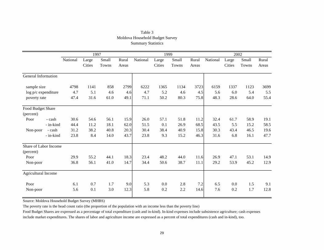
socio-economic status, etc.). Table 3 provides some characteristics of the data for 1997,
1999 and 2002.
Sample sizes are as follows: 4,798 households were interviewed in 1997, 6,219 in 1999,
and 6,159 in 2002. In 2002, the largest fraction of households resided in Rural Areas, where
13

approximately 60 percent of the population lived. 21.7 percent of the population lived in
Large Cities and the remaining 18.3 percent in Small Towns. These shares have not changed
much from 1997 to 2002.
The richest region is Large Cities, followed by Rural Areas and Small Towns. The
Moldovan economy collapsed in 1999 (after the Russian crisis) and recovered in 2002 after
two years of rapid growth. The head count ratio reacted strongly, raising to 71.1 percent in
1999 and dropping to 48.3 percent in 2002. Poverty is more prevalent in Small Towns than
in Rural Areas, a fact typically explained by the subsistence agricultural activities that are
available in rural areas.
In the model, I identified three channels through which trade affects household income:
consumption of food, labor income and net agricultural income. In 2002, the national share
of the budget spent on food (both cash and in-kind) was 75.9 percent for the poor and 61.9
percent for the non-poor. The share of cash food expenditures was 32.4 percent for the poor
and 30.3 percent for the non-poor. Notice, however, that there is substantial variation in
these shares for household residing in different regions. For example, while the cash food
share of the poor was 19.1 percent in rural areas, it was 61.7 percent in large cities. In
contrast, the in-kind food share of the poor was 58.5 percent in rural areas and 5.5 percent
in large cities. The total cash and in-kind food share of the poor was 67.2 percent in Large
Cities, 77.6 percent in Rural Areas, and 74.1 percent in Small Towns. Lower budget shares
were observed among the non-poor.
The share of labor income on total expenditure was 26.9 percent for the poor and 29.2
percent for the non-poor. Once again, there is substantial variation across regions, from 14.9
percent for the poor in rural areas, to 53.9 percent for the non-poor in large cities. Similar
differences are observed in terms of agricultural income, from 1.5 percent for the average
poor household in small towns to 12.8 percent for average non-poor household in rural areas.
Since the surveys have been collected monthly since April 1997, the data comprise a large
time series of household data that I combine with monthly price information published by the
Department of Statistics and Sociology of the Republic of Moldova. These price data refer
to a monthly index price of agro-industrial products related to agro-manufacturing export
14
markets.
4.2 Estimation
To estimate the labor income elasticities, I assume that the regression function for wages
can be written as
(15) lnwjt = α+L
l=0
βwl ln pt−l + pIγ + g xjtγw + ujt,
where wjt is the wage income of household j at time t, pt is the price faced by firms at t
(these prices are the same for all households interviewed in the same month t), and ujt is
an error term. Since wages will be affected not only by export prices but also by the prices
of other tradable goods, I introduce a vector of these prices pI in (15) too. For the sake
of generality, the effects of the other controls xjt, such as technical change and individual
characteristics, are captured by the function g(·). In (15), I introduce some dynamics inwage adjustments, so that wjt depends on current prices pt as well as on lagged prices, pt−l,
for lag l = 0 to L, the maximum number of lags. The long-run elasticitity of wages to prices
is given by δw =L
l=0
βwl .12
One problem in implementing the regression model (15) is that wages and prices may
be variables that are integrated of order one, I(1). This means that the regression in levels
may be subject to the problem of spurious regression, thereby estimating a statistically
significant relationship when none actually exists. Since Moldova suffered from moderate to
high inflation during this period, this is indeed a problem.
The standard solution is to estimate the model in first differences, but this is not
straightforward in the present case because I am using a time series of cross-sectional data.
This implies that the data vary not only across time t, but also across household units, j.
In what follows, I propose a procedure to remove the potential spurious correlation. The
12Notice that the prices of agricultural exports, pm, and of importable goods, pI , are assumed to beexogenous in (15). The implicit assumption, as argued in the theoretical model, is that Moldova is a verysmall country (with 3.5 million inhabitants and a per capita GDP of around 2000 US dollars). It is reasonableto argue, therefore, that exporters act as price takers.
15
procedure, which adapts techniques used in panel data models (Hsiao, 1986), comprises
differencing the model at t with respect to the average at t− 1. Specifically, notice that theaverage wage at t− 1 is
(16) lnwt−1 = α+L
l=0
βwl ln pt−l−1 +1
nt−1 j
g xjt−1γw + ut−1,
where a bar over a variable represents its average across j and nt−1 is the number of
observations at t−1. Assuming that wjt in (15) is I(1) with prices, and that wt−1 and pricesin (16) are integrated as well, I can generate a model with I(0) variables by subtracting (16)
from (15). This gives the following regression model
(17) lnwjt − lnwt−1 =L
l=0
βwl (ln pt−l − ln pt−l−1) + zjtγw + vwjt,
where vwjt = ujt − ut−1. At this stage, I adopt for simplicity a linear specification for thevector of controls, zjt. This vector includes variables such as age, age squared, education,
regional dummies, year dummies, plot size and trends; seasonal variables, such as monthly
or quarterly dummies are included as well. This model is free from the spurious regression
problem so that the parameter vector and the variance can be consistently estimated with
OLS. Exogeneity of export prices is required, too. Since Moldova is such a small economy, it
seems reasonable to assume that prices are set in international markets and that Moldovan
firms are price takers.
I set up a similar model to estimate the response of agricultural cash income
(18) ln ajt − ln at−1 =L
l=0
βal (ln pt−l − ln pt−1−l) + zjtγa + vajt.
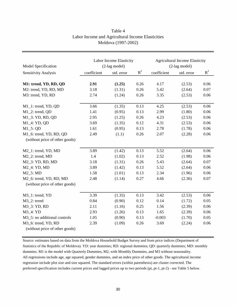
Results are in Table 4. In the upper panel, I report the estimates from a baseline specification
that includes all the regressors mentioned above and two lags (see below for details). The
main finding is that the price of agro-industrial goods impacts positively on wages. The
long-run elasticity, δw = β0 + β1 + β2, is 2.91 when quarterly dummies are included. If
16
monthly dummies are used instead, the elasticity is 3.18; without monthly or quarterly
dummies the elasticity is 2.74. As explained, higher export prices cause firms to expand
and to hire more workers, pushing wages up as a result. The elasticities are statistically
significant. The standard errors of the coefficients are corrected by the clustering that may
arise when aggregate variables (like prices pt) are used to explain individual variables, like
wages (Kloek, 1981).
In Table 4, I carry out some sensitivity analysis: for each seasonal model (i.e. quarterly
dummies, monthly dummies, and no seasonality) I run the regressions including different sets
of regressors. In all cases, the wage elasticities are positive, greater than one, and significant.
Including quarterly dummies or monthly dummies to account for seasonality in labor markets
that does make a differences. Excluding the seasonal controls and the year dummies, instead,
tends to make the elasticities lower. The exclusion of the prices of other tradable goods tends
to depress the estimates as well. The results are robust to the inclusion of the other controls
in z. In what follows I work with the specification that includes quarterly dummies and the
prices of other traded goods.
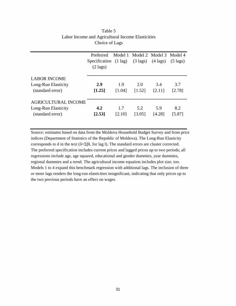
The choice of lags remains to be discussed. My strategy is to estimate the model including
a successively larger number of lags, starting with one lag and up to five lags, and to compare
the long-run elasticities. Table 5 reports these long-run elasticities. For the case of wages,
I find that the elasticities are positive and significant when one and two lags are included,
but become insignificant when three or more lags are added. This means that only prices up
to the two previous periods are affecting wages and that prices beyond that are not causing
any further wage change. I therefore adopt the two-lag specification in the poverty analysis
of section 5.
Tables 4 and 5 report results for the agricultural income specification. It turns out that
the prices of agro-manufactures do not affect significantly the cash crop income of Moldovan
families. There are several factors that help explain this result. Most importantly, I believe
that agriculture is a long-run activity and, consequently, decisions to grow and sell crops may
be done well in advance on a number of considerations that I am unable to control for in
the regressions. In any case, a systematic relationship between cash crop and agro-industrial
17
prices could not be found.
5 The Poverty Impacts
Based on equation (14), the estimated change in household welfare is
(19) ∆W j = αjwεwpm + αjaεapm − αjoutεwpm + sjm ∆ ln pm.
Given the results reported in Table 4, I adopt the value of εwpm = 2.91 for the estimated wage
price-elasticity. Since agricultural income appears not to significantly respond to prices, I
omit these effects in the rest of the paper. Budget shares (sjm) and income shares (αjw, α
ja,
and αjout) can be recovered for each household directly from the Moldovan Household Budget
Survey data.
The policy exercise investigated in this paper is a removal of some of the barriers that
impede trade in Moldova. There are two issues to consider in the estimation of the price
change, ∆ ln pm. One key issue is how changes in barriers are translated into changes in
prices. In the absence of suitable data to estimate a pass-through function, I work with
simulated changes in prices under two pass-through assumptions, full pass-through, and 50
percent pass-through. The second issue is that the informal barriers described in section 2
are different in nature. Some barriers, such as cumbersome regulations, can in principle be
easily removed; reducing others, such as transport costs, is more costly. To account for this
asymmetry, I assume different rates of reductions for different barriers.
5.1 The Distribution of the Welfare Effects
In this section, I use estimates of (19) to study the distribution of the welfare effects across
income levels. For this purpose, I assume that all informal barriers are halved so that trade
costs decline from 24.5 to 12.2 percentage points. Under my two pass-through assumptions, I
compute two price changes, ∆ ln pm = 12.3 (full pass-through) and ∆ ln pm = 6.2 (50 percent
pass-through), and I estimate two welfare effects, equation (19), for each household surveyed
18
in 2002. To study the distribution of these welfare effects, I estimate the average effect,
conditional on the level of per capita expenditure. These are useful measures because these
averages show the impact of a price change on a social welfare function (Deaton, 1989b), thus
indicating the welfare effects of the export barriers. To compute the averages at different
income levels, a locally weighted non-parametric procedure is adopted. In particular, I use
the local smoother proposed by Fan (1992) and Fan (1993).13
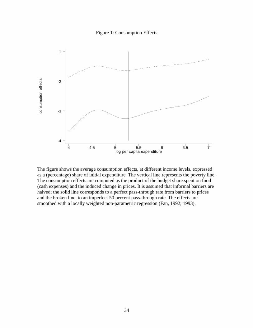
Figure 1 shows the welfare effects on the consumption side. The solid line plots the effects
under a full pass-through, and the broken line, those under a 50 percent pass-through. Since
the removal of export barriers raises domestic prices of food items, there are losses across all
income levels. These losses range from nearly 4 percent of initial expenditure for the poorest
households under a full pass-through, to around 1.5 percent for the richest households and
a 50 percent pass-through. At the poverty line (the vertical line in Figure 1), the average
losses reach between 1.8 to 3.2 percent.
There is a interesting pattern in the consumption effects that is worth mentioning.
Since, due to Engel law, the budget share spent on food is an decreasing function of total
expenditure, larger losses are expected for poorer households. This is observed in Figure 1,
with a caveat: the losses decline with expenditure at the very bottom of the distribution,
then increase with expenditure until the poverty line is reached, and finally decline again with
expenditure. To interpret this result, recall that most of the food consumption of households
in Rural Areas (mostly in the lower and intermediate range of per capita expenditure) is
in-kind, produced at the home plot (see Table 3). This implies a lower share spent on cash
food expenses for these families and lower welfare effects at middle income levels.
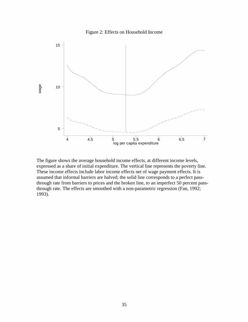
Figure 2 shows the average household income effects, i.e. the average change in the labor
income of the household, net of wage payments in cash agricultural production activities, as
a share of expenditure (estimated with a locally weighted Fan regression). I estimate average
welfare gains for households across the entire income distribution. The distribution of the
gains displays a U shape, with the gains declining with expenditure to the left of the poverty
line and increasing with expenditure to the right. The gains start at between 12.5 percent
13In all the applications of Fan regressions in this paper, I use a Gaussian Kernel with a bandwidth equalto 0.25. A discussion of nonparametric methods is in Appendix 1.
19

(in the full pass-through case) and 6 percent (in the 50 percent pass-through case) at the
bottom of the distribution and sharply decline with per capita expenditure until reaching
between 9 and 4 percent, respectively, in a boundary around the poverty line. As per capita
expenditure increases, the gains grow to between 14 and 6 percent of expenditure at the top
of the distribution.
The sources of the income gains from lower informal export barriers are reported in
Figures 3 and 4. Recall that wages positively respond to a reduction in trade barriers, while
agricultural income does not significantly react. Thus, Figure 3 displays the labor income
effects only. The U-shaped curve is evident here. For an explanation, recall that the share
of labor income is larger in Small Towns and in Large Cities (where poorest and richest
households reside, respectively) than in Rural Areas (where low to intermediate-income
households live).
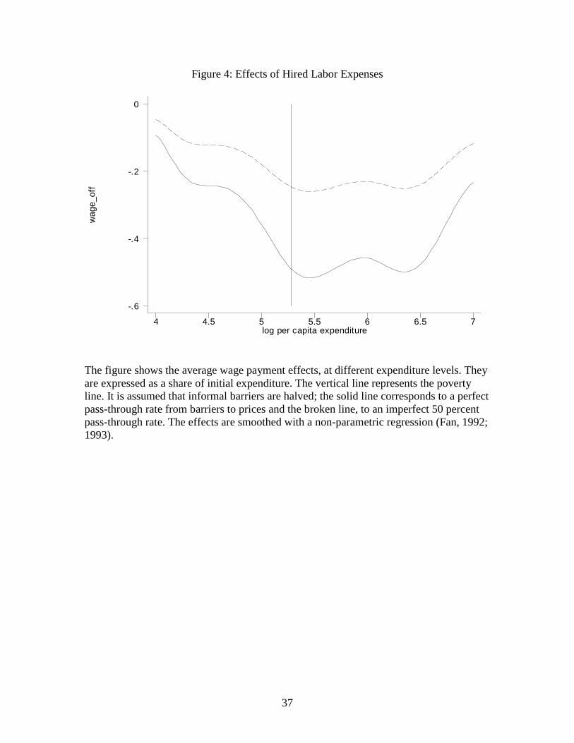
Figure 4 shows the distribution of the effects caused by having to pay higher wages to
hired labor. There are losses across the entire income distribution, and these losses tend
to be higher as per capita expenditure increases. This is probably related to the fact that
middle income to rich households tend to be endowed with more land and are therefore more
likely to be engaged in cash crop agricultural production (as opposed to subsistence) and
in hiring outside labor. Notice, however, that the positive income effects of receiving higher
induced wages are much larger than the costs of having to pay higher wages to outside labor.
As a result, the net income effects in Figure 2 are positive and display a U shape.
Figure 5 shows the total aggregate effect, the difference between the factor income effects
and the consumption effects. The net effects resemble the patterns observed in Figure 2.
This is another instance in which the impacts of trade on the income side dominate the
impacts on the consumption side. In theory, this is due to the magnification effects of
Jones. In practice, similar patterns have been found in Porto (2003a), Leamer (1996) and
Grossman and Levinsohn (1989), among others. In the Moldovan case, the result is explained
by a elastic response of wages to agro manufacturing prices (a version of the magnification
effects) and by the increase in the domestic price arising from lower informal barriers to
export.
20

5.2 Poverty Impacts
In 2002, 48.3 percent of the Moldovan population lived in poverty with a per capita
expenditure below the poverty line (estimated at 196.03 lei - approximately 15 US dollars -
per month). The poverty impacts of reducing export barriers can be carried out by comparing
head count ratios. I begin with an experiment in which the costs imposed by informal
barriers that impede trade are halved. Poverty would reach 43.3 percent, in the case of full
pass-through from barriers to prices, or 45.5 percent, in the case of imperfect pass-through.
This reduction of between 2.8 and 5 percentage points in the head count ratio involves lifting
around 100,000-180,000 Moldovans out of poverty. In a country with 3.5 million inhabitants
and 1.7 million poor individuals, these are large impacts.
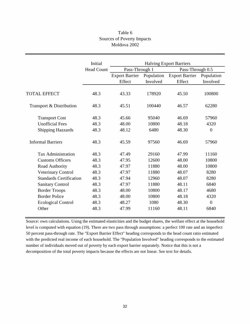
In Table 6, I report the individual poverty impacts by source of informal export barriers.
Notice that this is not a decomposition of the total poverty impacts because these effects
are not linear. Both Transport and Distribution (T&D) and Informal Barriers (IB) have
similar impacts on poverty. Halving T&D costs would cause poverty to decline by between
62,000 and 100,000 individuals; most of these impacts are caused by transport, handling and
insurance. Halving IB costs would move between 58,000 and 98,000Moldovans out of poverty.
In order of importance among the IB items, the impacts are caused by Tax Administration,
Customs Officers, Road Authority, Veterinary Control, Standards Certification, Sanitary
Controls, Border Troops and Border Police.
Notice that the poverty impacts vary a lot by source of trade barrier. This is expected
since the effects of removing each barrier depend on its initial level. In particular, transport
costs are by far the most important trade barriers; by themselves, they cause roughly the
same poverty effects that all the other informal barriers (IB in the second panel of Table 6)
together. Since some poverty barriers are easier to remove than others, it is important to
perform a simple sensitivity analysis of the poverty impacts for different assumptions about
the changes in informal barriers. This analysis is reported in Table 7.
The first column of the table shows the initial head count, 48.3 percent. In columns 2
and 3, I report the poverty impacts of reducing export barriers by 25 percent under perfect
and imperfect pass-through rates. In columns 4 and 5, I repeat the exercise under an
21
assumed 10 percent reduction in trade barriers. The poverty impacts are now lower. With
perfect pass-through and a 25 percent reduction in all barriers, the head count would be 45.5
percent (2.8 percentage points lower than the initial head count). Instead, with a 10 percent
reduction in all barriers and an imperfect pass-through, poverty would decline by only 0.7
percentage points. As expected, transport costs are the most important trade barrier, but
the total effects of reducing all other informal barriers (IB) are similar in magnitude. Even
if trade barriers are reduced by only 10 percent, so that many of the partial effects of the IB
components are very small (see column 5, for instance), the combined effect of all Informal
Barriers is still important.
In columns 6 and 7, I combine a reduction of 10 percent in T&D with a 25 percent
reduction in IB to capture the fact that transport costs are much more costly to improve than
informal barriers. Since for a given rate of barrier reduction, improvements in transport costs
have roughly the same impacts as improvements in all informal barriers, it is not surprising
to find larger impacts for IB reduction in this exercise. Under perfect pass-through, T&D
would bring the head count to 47.60 and IB, to 46.69. For imperfect pass-through, T&D
would bring the poverty rate to 47.97, while IB, to 47.49. The total effect would bring
the head count from 48.3 percent to 46.1 percent (under perfect pass-through) or to 47.1
percent (under imperfect pass-through). These results provide some support to the claim
that attacking IB can be as effective as attacking more standard forms of trade facilitation
barriers, such as transport costs.14
6 Conclusions
While most of the current literature on trade and poverty focuses on the impacts of formal
trade liberalization, in this paper I have emphasized a novel, and previously unexplored,
aspect of international trade. This is the role of informal export barriers such as transport
costs, cumbersome customs practices, costly regulations, and bribes. In a world where formal
trade barriers are being eliminated, these informal impediments to trade are beginning to
14Notice that such a claim only makes sense if a complete cost benefit analysis is carried out. This is notmy purpose in this paper, though.
22
receive more attention both from researchers and policy makers.
I have investigated the poverty impacts of improving export practices in Moldova, a poor
country with a comparative advantage in agriculture. Moldova is a very open economy that
relies heavily on external markets to develop and grow. Whereas formal trade barriers (tariffs,
quotas, export taxes) are fairly low, informal trade barriers are high. I have found that
improving transport infrastructure, fighting corruption, and improving customs practices
would have a large poverty alleviation impact. By cutting informal costs by half, the poverty
rate would decline from an initial head count ratio of 48.3 percent, to between 43.3 and 45.5
percent. If lower reductions in trade barriers are assumed (such as reducing barriers by 10
to 25 percent), the poverty impacts would still be important, with a reduction of 0.7 to 2.8
percentage points. Transport costs are the most important trade facilitation barrier. But
the combined effect of other informal barriers, such as customs practices, tax paperwork,
bribes of government officials, and regulations, can be as important.
The large impacts on poverty found in this paper suggest that the government should
seriously consider programs to cut informal barriers to trade and pursue a better business
environment. In principle, it would be interesting to investigate the differential effects of
formal versus informal barriers to trade as well. Such analysis could provide additional
valuable guidelines for policy reforms in developing countries. Since Moldova faces low
formal barriers, it is not the most appropriate scenario to study these matters. But the
question is important and remains open for future research.
Appendix 1. Non-Parametric Regressions
As opposed to a standard regression model, nonparametric regressions do not impose thelinearity assumption on the conditional expectation. The technique attempts to recover amuch richer relationship between the dependent variable and the explanatory variable. Fan(1992, 1993) proposed a locally weighted regression model that approximates the regressionfunction for the average welfare effects E[∆W j|x] at different income levels x. Intuitively,Fan regressions are linear regressions at each x that weigh observations with a kernel functionin order to give more importance to data points closer to x.At x, the Fan regressions solve
minα,β
j
∆W j − α− β(xj − x)2
Kxj − xh
.
23
The bandwidth h defines the local data used in the non-parametric regression. In theapplications in the text, h was chosen by visual inspection. The function K(·) represents thekernel function that attaches weights to different observations. The choice of kernels is nottoo important; in this paper I use Gaussian kernels.Intuitively, one way to estimate the local averages would be by computing averages of
the dependent variable at different levels of the explanatory variable. In general, though,there would be a very small numbers of observations at each x. The non-parametricregression model estimates these averages using all the data in the sample and giving weightsaccording to the kernel function. Specifically, for each datum along the income distribution,observations closer to x should receive a greater weight than observations farther away. Thisis exactly what the Fan regressions do. Notice that the combination of local regressions withkernel smoothing allows the non-parametric regression to be locally design adaptive. Thismeans that the regression adapts to the design of the random sample and therefore its biasdoes not depend on the density (or the derivative of the density function) of the pre-selectedpoint x.
References
Anderson, J., van Wincoop, E., 2003. Trade Costs. Journal of Economic Literature,
forthcoming.
Attanasio, O., Goldberg, P., Pavcnik, N., 2004. Trade Reforms and Income Inequality in
Colombia. Journal of Development Economics, forthcoming.
Benjamin, D., 1992. Household Composition, Labor Markets, and Labor Demand: Testing
for Separation in Agricultural Household Models. Econometrica 60, 287-322.
Deaton, A., 1989a. Rice Prices and Income Distribution in Thailand: a Non-Parametric
Analysis. Economic Journal 99, 1-37.
Deaton, A., 1989b. Household Survey Data and Pricing Policies in Developing Countries.
The World Bank Economic Review 3, 183-210.
Deaton, A., 1997. The Analysis of Household Surveys. A Microeconometric Approach to
Development Policy. John Hopkins University Press for the World Bank.
Dixit, A., Norman, V., 1980. Theory of International Trade. A Dual, General Equilibrium
Approach. Cambridge Economic Handbooks.
24
Edmonds, E., Pavcnik, N., 2004a. The Effects of Trade Liberalization on Child Labor.
Journal of International Economics, forthcoming.
Edmonds, E., Pavcnik, N., 2004b. Trade Liberalization and Household Labor Supply in a
Poor Country: Evidence from Vietnam. Dartmouth College mimeo.
Fan, J., 1992. Design-adaptive nonparametric regression. Journal of the American Statistical
Association 87, 998-1004.
Fan, J., 1993. Local Linear Regression Smoothers and Their Minimax Efficiencies. Annals of
Statistics 21, 196-216.
Feenstra, R.C., 2004. Advanced International Trade: Theory and Evidence. Princeton
University Press, Princeton.
Friedman, J., Levinsohn, J., 2002. The Distributional Impacts of Indonesia’s Financial Crisis
on Household Welfare: A ‘Rapid Response’ Methodology. World Bank Economic Review 16,
397-423.
Goldberg, P., Pavcnik, N., 2003. The Response of the Informal Sector to Trade Liberalization.
Journal of Development Economics 72, 463-496.
Goldberg, L., Tracy, J., 2003. Exchange Rates and Wages. Federal Reserve Bank of New
York, mimeo.
Grossman, G., Levinsohn, J., 1989. Import Competition and the Stock Market Return to
Capital. American Economic Review 198, 1065-1087.
Hsiao, C., 1986. Analysis of Panel Data. Econometric Society Monographs No 11, Cambridge
University Press.
Kloek, T., 1981. OLS Estimation in a Model Where a Microvariable is Explained
by Aggregates and Contemporaneuos Disturbances are Equicorrelated. Econometrica 49,
205-207.
Leamer, E., 1996. In Search of Stolper-Samuelson Effects on US Wages. NBER WP5427.
25

Ministry of Economy of the Republic of Moldova, 2003. Regulatory Cost Assessment Survey
in Moldova, Chisinau, Moldova.
Porto, G., 2003. Using Survey Data to Assess the The Distributional Effects of Trade Policy.
Policy Research Working paper, the World Bank Research Group.
Singh, I., Squire, L., Strauss, J., eds., 1985. Agricultural Household Models: Extensions,
Applications and Policy, Baltimore, Johns Hopkins Press for the World Bank.
Woodland, A., 1982. International Trade and Resource Allocation, Advanced Textbooks in
Economics, vol. 19, North Holland, Amsterdam.
Wolak, F., 1996. The Welfare Impacts of Competitive Telecommunications Supply: A
Household-Level Analysis. Brookings Papers on Economic Activity Microeconomics, 269-340.
World Bank, 2003. Exporter and Importer Survey in Moldova, Washington DC.
26
Destination Transport Unofficial Shipping Totalof exports Cost Fees Hazards
CIS 13.7 1.3 0.5 15.5
EU 7.7 0.1 0.1 7.9
Other 11.3 0.2 11.5
Total 11.6 0.7 0.3 12.6
Source: own calculations based on the Exporter and ImporterWorld Bank Survey (2003).Transport Costs: freight, handling & insuranceUnofficial Fees: bribes paid on transitShipping Hazards: damaged or stolen goods during on transitAll figures represent percentages of the value of an export shipmentCIS: Commonwealth of Independent States (Russia, Ukraine, etc.)EU: European Union
Table 1Transportation, Shipping and Distribution Costs
(percent of export shipment)
27
Domestic Ukraine Total
Tax Administration 2.78 0.00 2.78Customs Officers 0.44 1.17 1.61Road Authority 0.50 0.77 1.27Veterinary Control 1.13 0.11 1.24Standards Certification 0.83 0.36 1.19Sanitary Control 0.76 0.23 0.99Border Troops 0.38 0.48 0.84Border Police 0.46 0.18 0.64Ecological Control 0.09 0.09 0.18Other 0.21 0.79 1.00
Total Average Cost 7.57 4.34 11.91
Source: Exporter and Importer Survey, World Bank (2003)All figures represent percentages of the value of an export shipment.Informal barriers comprise unofficial fees and bribes paid to thedifferent government units listed in the table. Domestic costs referto amounts paid to Moldovan officials; Ukraine costs refer topayments to Ukrainian officials and individuals. Since Moldova is alandlocked country, export shipments to Russia (the main exportdestination) have to travel through Ukraine.
Table 2The Cost of Informal Export Barriers
(percent of export shipment)
28
National Large Small Rural National Large Small Rural National Large Small RuralCities Towns Areas Cities Towns Areas Cities Towns Areas
General Information
sample size 4798 1141 858 2799 6222 1365 1134 3723 6159 1337 1123 3699 log p/c expenditure 4.7 5.1 4.6 4.6 4.7 5.2 4.6 4.5 5.6 6.0 5.4 5.5 poverty rate 47.4 31.6 61.0 49.1 71.1 50.2 80.3 75.8 48.3 28.6 64.0 55.4
Food Budget Share(percent) Poor - cash 30.6 54.6 56.1 15.9 26.0 57.1 51.8 11.2 32.4 61.7 58.9 19.1 - in-kind 44.4 11.2 18.1 62.0 51.5 0.1 26.9 68.5 43.5 5.5 15.2 58.5 Non-poor - cash 31.2 38.2 40.8 20.3 30.4 38.4 40.9 15.8 30.3 43.4 46.5 19.6 - in-kind 23.8 8.4 14.0 43.7 23.8 9.3 15.2 46.3 31.6 6.8 16.1 47.7
Share of Labor Income(percent) Poor 29.9 55.2 44.1 18.3 23.4 48.2 44.0 11.6 26.9 47.1 53.1 14.9 Non-poor 36.8 56.1 41.0 14.7 34.4 50.6 38.7 11.1 29.2 53.9 45.2 12.9
Agricultural Income
Poor 6.1 0.7 1.7 9.0 5.3 0.0 2.8 7.2 6.5 0.0 1.5 9.1 Non-poor 5.6 0.1 3.0 12.3 5.8 0.2 2.2 14.6 7.6 0.2 1.7 12.8
Source: Moldova Household Budget Survey (MHBS)
The poverty rate is the head count ratio (the proportion of the population with an income less than the poverty line)
Food Budget Shares are expressed as a percentage of total expenditure (cash and in-kind). In-kind expenses include subsistence agriculture; cash expenses
include market expenditures. The shares of labor and agriculture income are expressed as a percent of total expenditures (cash and in-kind), too.
1997 1999 2002
Table 3Moldova Household Budget Survey
Summary Statistics
29
Model Specification
Sensitivity Analysis coefficient std. error R2 coefficient std. error R2
M1: trend, YD, RD, QD 2.91 (1.25) 0.26 4.17 (2.53) 0.06M2: trend, YD, RD, MD 3.18 (1.31) 0.26 5.42 (2.64) 0.07M3: trend, YD, RD 2.74 (1.24) 0.26 3.35 (2.53) 0.06
M1_1: trend, YD, QD 3.66 (1.35) 0.13 4.25 (2.53) 0.06M1_2: trend, QD 1.41 (0.95) 0.13 2.99 (1.80) 0.06M1_3: YD, RD, QD 2.95 (1.25) 0.26 4.23 (2.53) 0.06M1_4: YD, QD 3.69 (1.35) 0.12 4.31 (2.53) 0.06M1_5: QD 1.61 (0.95) 0.13 2.78 (1.78) 0.06M1_6: trend, YD, RD, QD 2.49 (1.1) 0.26 2.07 (2.28) 0.06 (without price of other goods)
M2_1: trend, YD, MD 3.89 (1.42) 0.13 5.52 (2.64) 0.06M2_2: trend, MD 1.4 (1.02) 0.13 2.52 (1.98) 0.06M2_3: YD, RD, MD 3.18 (1.31) 0.26 5.43 (2.64) 0.07M2_4: YD, MD 3.89 (1.42) 0.13 5.52 (2.64) 0.06M2_5: MD 1.58 (1.01) 0.13 2.34 (1.96) 0.06M2_6: trend, YD, RD, MD 2.48 (1.14) 0.27 4.66 (2.36) 0.07 (without price of other goods)
M3_1: trend, YD 3.39 (1.35) 0.13 3.42 (2.53) 0.06M3_2: trend 0.84 (0.90) 0.12 0.14 (1.72) 0.05M3_3: YD, RD 2.11 (1.16) 0.25 1.56 (2.39) 0.06M3_4: YD 2.93 (1.26) 0.13 1.65 (2.39) 0.06M3_5: no additional controls 1.05 (0.90) 0.13 -0.003 (1.70) 0.05M3_6: trend, YD, RD 2.39 (1.09) 0.26 3.69 (2.24) 0.06 (without price of other goods)
Source: estimates based on data from the Moldova Household Budget Survey and from price indices (Department of
Statistics of the Republic of Moldova). YD: year dummies; RD: regional dummies; QD: quarterly dummies; MD: monthly
dummies. M1 is the model with Quarterly Dummies, M2, with Monthly Dummies, and M3 without seasonality.
All regressions include age, age squared, gender dummies, and an index price of other goods. The agricultural income
regression include plot size and size squared. The standard errors (within parenthesis) are cluster corrected. The
preferred specification includes current prices and lagged prices up to two periods (pt, pt-1, pt-2) - see Table 5 below.
(2-lag model)
Table 4Labor Income and Agricultural Income Elasticities
Moldova (1997-2002)
Labor Income Elasticity Agricultural Income Elasticity(2-lag model)
30
Preferred Model 1 Model 2 Model 3 Model 4Specification (1 lag) (3 lags) (4 lags) (5 lags)
(2 lags)
LABOR INCOMELong-Run Elasticity 2.9 1.9 2.0 3.4 3.7 (standard error) [1.25] [1.04] [1.52] [2.11] [2.78]
AGRICULTURAL INCOMELong-Run Elasticity 4.2 1.7 5.2 5.9 8.2 (standard error) [2.53] [2.10] [3.05] [4.28] [5.87]
Source: estimates based on data from the Moldova Household Budget Survey and from priceindices (Department of Statistics of the Republic of Moldova). The Long-Run Elasticitycorresponds to d in the text (δ=Σβl, for lag l). The standard errors are cluster corrected.The preferred specification includes current prices and lagged prices up to two periods; allregressions include age, age squared, educational and gender dummies, year dummies,regional dummies and a trend. The agricultural income equation includes plot size, too.Models 1 to 4 expand this benchmark regression with additional lags. The inclusion of threeor more lags renders the long-run elasticities insignificant, indicating that only prices up tothe two previous periods have an effect on wages.
Table 5Labor Income and Agricultural Income Elasticities
Choice of Lags
31
InitialHead Count
Export Barrier Population Export Barrier PopulationEffect Involved Effect Involved
TOTAL EFFECT 48.3 43.33 178920 45.50 100800
Transport & Distribution 48.3 45.51 100440 46.57 62280
Transport Cost 48.3 45.66 95040 46.69 57960 Unofficial Fees 48.3 48.00 10800 48.18 4320 Shipping Hazzards 48.3 48.12 6480 48.30 0
Informal Barriers 48.3 45.59 97560 46.69 57960
Tax Administration 48.3 47.49 29160 47.99 11160 Customs Officers 48.3 47.95 12600 48.00 10800 Road Authority 48.3 47.97 11880 48.00 10800 Veterinary Control 48.3 47.97 11880 48.07 8280 Standards Certification 48.3 47.94 12960 48.07 8280 Sanitary Control 48.3 47.97 11880 48.11 6840 Border Troops 48.3 48.00 10800 48.17 4680 Border Police 48.3 48.00 10800 48.18 4320 Ecological Control 48.3 48.27 1080 48.30 0 Other 48.3 47.99 11160 48.11 6840
Source: own calculations. Using the estimated elasticities and the budget shares, the welfare effect at the household
level is computed with equation (19). There are two pass through assumptions: a perfect 100 rate and an imperfect
50 percent pass-through rate. The "Export Barrier Effect" heading corresponds to the head count ratio estimated
with the predicted real income of each household. The "Population Involved" heading corresponds to the estimated
number of individuals moved out of poverty by each export barrier separately. Notice that this is not a
decomposition of the total poverty impacts because the effects are not linear. See text for details.
Pass-Through 1 Pass-Through 0.5
Table 6Sources of Poverty Impacts
Moldova 2002
Halving Export Barriers
32

InitialHead Count
Pass-T=1 Pass-T=0.5 Pass-T=1 Pass-T=0.5 Pass-T=1 Pass-T=0.5
TOTAL EFFECT 48.3 45.50 46.69 47.07 47.60 46.11 47.16
Transport & Distribution (T&D) 48.3 46.57 47.43 47.60 47.97 47.60 47.97
Transport Cost 48.3 46.69 47.49 47.62 47.97 47.62 47.97 Unofficial Fees 48.3 48.18 48.27 48.30 48.30 48.30 48.30 Shipping Hazzards 48.3 48.30 48.30 48.30 48.30 48.30 48.30
Informal Barriers (IB) 48.3 46.69 47.49 47.62 47.94 46.69 47.49
Tax Administration 48.3 47.99 48.00 48.11 48.24 47.99 48.00 Customs Officers 48.3 48.00 48.18 48.18 48.27 48.00 48.18 Road Authority 48.3 48.00 48.18 48.24 48.30 48.00 48.18 Veterinary Control 48.3 48.07 48.18 48.24 48.30 48.07 48.18 Standards Certification 48.3 48.07 48.18 48.24 48.30 48.07 48.18 Sanitary Control 48.3 48.11 48.24 48.27 48.30 48.11 48.24 Border Troops 48.3 48.17 48.24 48.27 48.30 48.17 48.24 Border Police 48.3 48.18 48.27 48.30 48.30 48.18 48.27 Ecological Control 48.3 48.30 48.30 48.30 48.30 48.30 48.30 Other 48.3 48.11 48.24 48.27 48.30 48.11 48.24
Source: own calculations as described in Table 6. There are three experiments in the table: a reduction of all barriers by 25 percent, a
reduction in all barriers by 10 percent, and a reduction of Transport and Distribution by 10 percent and a reduction of Informal Barriers by
25 percent. For each of these cases, a perfect pass-through and an imperfect 50 percent pass-through are considered.
The Head Count ratio is the proportion of the population in poverty (i.e. with a per capita expenditure below the poverty line)
IB by 25%Reducing Barriers by 25% Reducing Barriers by 10%
Table 7Sources of Poverty Impacts: Some Sensitivity
Moldova 2002
Reducing T&D by 10% and
33
34
Figure 1: Consumption Effects
co
nsum
ptio
n ef
fect
s
log per capita expenditure4 4.5 5 5.5 6 6.5 7
-4
-3
-2
-1
The figure shows the average consumption effects, at different income levels, expressed as a (percentage) share of initial expenditure. The vertical line represents the poverty line. The consumption effects are computed as the product of the budget share spent on food (cash expenses) and the induced change in prices. It is assumed that informal barriers are halved; the solid line corresponds to a perfect pass-through rate from barriers to prices and the broken line, to an imperfect 50 percent pass-through rate. The effects are smoothed with a locally weighted non-parametric regression (Fan, 1992; 1993).
35
Figure 2: Effects on Household Income
wag
e
log per capita expenditure4 4.5 5 5.5 6 6.5 7
5
10
15
The figure shows the average household income effects, at different income levels, expressed as a share of initial expenditure. The vertical line represents the poverty line. These income effects include labor income effects net of wage payment effects. It is assumed that informal barriers are halved; the solid line corresponds to a perfect pass-through rate from barriers to prices and the broken line, to an imperfect 50 percent pass-through rate. The effects are smoothed with a non-parametric regression (Fan, 1992; 1993).

36
Figure 3: Labor Income Effects
inco
me
log per capita expenditure4 4.5 5 5.5 6 6.5 7
5
10
15
The figure shows the average household labor income effects, at different income levels. They are expressed as a share of initial expenditure. The vertical line represents the poverty line. It is assumed that informal barriers are halved; the solid line corresponds to a perfect pass-through rate from barriers to prices and the broken line, to an imperfect 50 percent pass-through rate. The effects are smoothed with a non-parametric regression (Fan, 1992; 1993).
37
Figure 4: Effects of Hired Labor Expenses
wag
e_of
f
log per capita expenditure4 4.5 5 5.5 6 6.5 7
-.6
-.4
-.2
0
The figure shows the average wage payment effects, at different expenditure levels. They are expressed as a share of initial expenditure. The vertical line represents the poverty line. It is assumed that informal barriers are halved; the solid line corresponds to a perfect pass-through rate from barriers to prices and the broken line, to an imperfect 50 percent pass-through rate. The effects are smoothed with a non-parametric regression (Fan, 1992; 1993).

38
Figure 5: Total Welfare Effects of Reducing Informal Export Barriers
tota
l
log per capita expenditure4 4.5 5 5.5 6 6.5 7
2
4
6
8
10
12
The figure shows the average household welfare effects, at different income levels. They are expressed as a share of initial expenditure. The vertical line represents the poverty line. The welfare effects include factor income effects (labor income net of wage payment on hired labor) net of consumption effects. It is assumed that informal barriers are halved; the solid line corresponds to a perfect pass-through rate from barriers to prices and the broken line, to an imperfect 50 percent pass-through rate. The effects are smoothed with a non-parametric regression (Fan, 1992; 1993).