influence of waves on lagrangian acceleration in two...

ESAIM: PROCEEDINGS, October 2011, Vol. 32, p. 231-241

E. Cances, N. Crouseilles, H. Guillard, B. Nkonga, and E. Sonnendrucker, Editors

INFLUENCE OF WAVES ON LAGRANGIAN ACCELERATION

IN TWO-DIMENSIONAL TURBULENT FLOWS ∗, ∗∗, ∗∗∗

Romain Nguyen van yen1, Benjamin Kadoch2, Vivek Kumar1, Benjamin

Menetrier1, Marie Farge1, Kai Schneider2, Diane Douady3 and Lionel Guez1

Abstract. The Lagrangian statistics in rotating Saint-Venant turbulence are studied by means of

direct numerical simulation using a pseudo-spectral discretization fully resolving, both in time and

space, all the inertio-gravity waves present in the system. To understand the influence of waves,

three initial conditions are considered, one which is dominated by waves, one which is dominated by

vortices, and one which is intermediate between these two extreme cases. It is found that Lagrangian

acceleration is strongly influenced by the presence of waves, as are the Lagrangian velocity increments,

for incremements that are sufficiently short, and that vortex motion influences mostly the component

of Lagrangian acceleration which is perpendicular to the local velocity.

1. Introduction

Among the many kinds of motion occuring in multiscale flows, the case of waves that are both fast enoughand small enough in amplitude is perhaps the best understood, since these waves can be described by expandingthe equations in terms of different time scales, a technique known as fast-slow splitting in singular perturbationtheory [2]. The rotating Saint-Venant equations (also called shallow water equations) in the limit of smallRossby number, i.e., for a referential rotating at a frequency larger than the flow vorticity, have been a toymodel for developing such approaches in weakly nonlinear regimes and understanding their properties. Werefer the reader to the textbook [16] for a self-contained tutorial on the subject. In the context of rotatingSaint-Venant, the splitting allows to average out fast inertio-gravity waves. As first realized by Rossby [12], inan appropriate parameter regime the slow component is described to first order in Rossby number by the quasi-geostrophic equations, which are completely independent on the behavior of the fast component. In particular,

∗ The authors thank the CIRM Marseille for its hospitality and for financial support during the CEMRACS 2010 Summer

Program where part of the work was carried out, and IDRIS-CNRS for providing computing facilities.∗∗ VK would like to thank the French embassy in India for financial support of his visit in ENS Paris, and EGIDE for all kind

of help.∗∗∗ RNVY, MF and KS are thankful to the Association CEA-EURATOM and to the French Research Federation for Fusion

Studies for supporting their work within the framework of the European Fusion Development Agreement and the French Research

Federation for Fusion Studies under the contract V.3258.001. This work is supported by the European Communities under the

contract of Association between Euratom and CEA. The views and opinions expressed herein do not necessarily reflect those

of the European Commission.1 LMD–CNRS, ENS, 24 rue Lhomond, 75231 Paris Cedex2 M2P2–CNRS & CMI Universites d’Aix–Marseille3 Departement de Mathematiques, Universite de Cergy

c© EDP Sciences, SMAI 2011

Article published online by EDP Sciences and available at http://www.esaim-proc.org or http://dx.doi.org/10.1051/proc/2011023

http://publications.edpsciences.org/

http://www.esaim-proc.org

http://dx.doi.org/10.1051/proc/2011023

232 ESAIM: PROCEEDINGS

this usually requires that the wave amplitude parameter, denoted λ from now on, is of the same order as theRossby number.

The aim of the work presented in this paper is to understand the effect of such waves on passively advectedpointwise massless particles, in the case where the vortical flow is in the fully developed turbulence regime,which is the most difficult to address analytically, since the separation of time scales between the waves andthe vortical flow becomes only marginally valid. As a first approach to this problem we choose the rotatingSaint-Venant equations, which are among the simplest models giving rise to both waves and turbulent motion.They are classically used to describe geophysical flows at the synoptic scale, since the Earth’s curvature and thenon-hydrostatic vertical motions can then be neglected. In atmospheric models, which aim to predict large scaleflows, it is essential to take into account gravity waves [9]. It has been shown [6] that both rotation and inertio-gravity waves reduce the nonlinear interactions between geostrophic vortices and thus inhibit the turbulentcascade for scales larger than the Rossby deformation radius. New ad-hoc models are still being activelydeveloped to improve over existing approximations [7], and it is thus important to improve our understandingof the effect of waves in this context. Other long term motivations for this work are magnetic confinement fusionwhich involves fast drift waves [5], and solar physics where fast magneto-gravity waves enter into play [13].

A famous example of impact of the waves on particles is the Stokes drift [14], which is formally of secondorder in terms of the wave amplitude. More comprehensive studies of the retroaction of the waves on meanLagrangian quantities have been performed since then (see e.g. [3]). On the other hand, the behavior of the fastfield may also be interesting for its own sake, in particular when considering quantities that are sensitive to highfrequency flow variations. The Lagrangian acceleration, on which we focus in this work, is one of them. Weclosely follow an approach which was previously applied to 2D incompressible turbulence [10] and 2D drift-waveturbulence [11]. As can be seen from a naive order of magnitude estimate, although the particle displacementdue to fast waves may be negligible because it is proportional to λ, the acceleration experienced by a particleduring the passage of a wave is proportional to ω2λ (where ω is a characteristic wave frequency) which is sureto become non-negligible for fast enough waves. However, as we shall see below, statistics previously observedin incompressible turbulence can be recovered in rotating Saint-Venant turbulence at the price of some timeintegration, or by direct observation of the Lagrangian velocity.

In the following, the rotating Saint-Venant equations are solved by direct numerical simulation, and tomaintain a high-level of turbulence the flow is initialized with random fields excited on a wide range of scales,and hyperdissipation is used to widen the inertial range. No external forcing term is applied to the flow. Severalnumerical simulations are performed with different levels of inertio-gravity waves and two rotation rates. Toadvect the particles, Eulerian velocity is computed at each time step, and bicubic interpolation is used. Wefirst report on the properties of the flows in the Eulerian reference frame as has been classically considered,and then we proceed with the results concerning the Lagrangian trajectories, which are the original part of ourwork. Finally we draw some overall conclusions.

2. Method

2.1. Dynamical model

To tackle this type of problems, we adopt an ab initio approach, which consists in solving numerically thefull rotating Saint-Venant system with spatial and temporal resolutions that are sufficiently fine to resolve allthe waves. The rotating Saint-Venant equations describe the flow of a thin incompressible fluid layer whichrotates at a constant rate and satisfies the following additional hypotheses:

- the fluid is in hydrostatic equilibrium with gravity,- all vertical gradients are negligible compared to horizontal gradients,- the thickness of the water layer is negligible compared with its characteristic horizontal size.

ESAIM: PROCEEDINGS 233

Under these hypotheses, conservation of mass and momentum imply the following system:

{λ∂th+ ∇ · (u(1 + λh)) = 0

∂tu + (u · ∇)u + 1

Roz × u− λ

k2

dRo2 ∇h = 0 (1)

where u(x, t) is the velocity field, the space variable x varies in a horizontal domain, z is the upward unitvector normal to this domain, h is the surface height perturbation, Ro is the Rossby number, kd is the Rossbydeformation wavenumber and λ is the nonlinearity parameter. Since the nonlinearities are bound to exciteever smaller spatial scales, we have to include some kind of dissipation mechanism to compensate. For thiswe employ the technique of hyperdissipation, both for the velocity equation and for the height perturbationequation, which consists in adding a term c∆8u (respectively c∆8h) on the right hand side of the respectiveequations for u and h. Compared to a standard dissipative term, this classical procedure [1] allows for a widerinertial range by concentrating dissipation at higher wavenumbers. To approximate homogeneous isotropic

turbulence, the equations are solved in the periodic domain T2 = (R/Z)

2. The choice of units that we have

made leads to the following link between the dimensionless numbers appearing in (1) and physical quantities:Ro = UL−1f−1, and λ = ∆HH−1

0 , where U is a characteristic velocity constructed from the total initial energy,

kd = Lf(gH0)−1/2, f/2 is the rotation frequency, g is the modulus of gravity, H0 is the height of the fluid at

rest, L is the size of the domain, and ∆H is the initial maximum height perturbation. Time is normalized bythe eddy turnover time LU−1.

In the absence of dissipation (c = 0), a remarkable property of solutions to the Saint-Venant equations isthat the potential vorticity

q =Ro−1 + ζ

1 + λh(2)

is conserved along Lagrangian trajectories, where ζ = ∇ × u is the vorticity of the flow in the rotating frameof reference (sometimes called relative vorticity). Moreover, these solutions have constant energy

E =1

2

∫

T2

((1 + λh)u2 +

λk−2d

Ro2h2

), (3)

and constant potential enstrophy

Zp =1

2

∫

T2

(Ro−1 + ζ)2

1 + λh. (4)

Since the energy is not a quadratic form in terms of the flow variables, the classical techniques of spectralanalysis used in turbulence cannot be directly applied. A quadratic invariant is recovered only in the limitwhere the Saint-Venant equations can be linearized around a rest state where velocity u = 0, and the heightperturbation vanishes. In this case, a convenient way of analyzing the flow consists in expanding it over theeigenmodes of this linearized system, which are given in Fourier space by:

u0(k) =ik⊥

k2d + k2

, h0(k) =k2

dRoλ−1

k2d + k2

, u±(k) = kd±k

√k2

d + k2 − ik⊥

2k2(k2d + k2)

and h±(k) =Roλ−1k2

dk2

2k2(k2d + k2)

,

where k is the wavenumber, and k⊥ is obtained by rotating k by π2. In the following, the projecton of the

flow over the eigenmodes indexed by 0 will be called “potentio-vortical flow”, while the residual part of theflow, corresponding to the projection over the eigenmodes indexed by ±, will be called “inertio-gravitational”,Since the eigenmodes are orthogonal, the total energy can be split in the same way into potentio-vortical andinertio-gravitational energies. In the nonlinear regime, the potentio-vortical and inertio-gravitational energiesare no longer constant, but the separation can still be carried out and yields information about the propertiesof the flow [6], which is meaningful as long as λ remains small.


A remarkable property of the rotating Saint-Venant equations is the tendency of their solutions, under someconditions, to approximately satisfy the geostrophic balance relation:

u ≈

(−∂y

∂x

)λh

k2dRo

.

This relation can also be visualized, as we shall do below, using the streamfunction ψ. The streamfunction ψand the velocity potential χ are both uniquely defined up to a constant by the Helmholtz decomposition of u:

u = z × ∇ψ + ∇χ,

and geostrophic balance then corresponds to

ψ ≈λh

k2dRo

and χ ≈ 0. (5)

The rotating Saint-Venant equations are discretized spatially using a pseudo-spectral method [4], and tem-porally using the leap-frog scheme, in order to preserve the dispersive properties of the inertio-gravity waves.All the results presented below were obtained in double precision and with a cut-off wavenumber of spatialdiscretization equal to 128, which amounts to using a collocation grid having N = 256 in each direction, orequivalently a mesh size π

128. The duration of the timestep is fixed throughout the computation to a value which

ensures numerical stability according to a CFL-type criterion based on the phase velocity of the fastest resolvedwaves. Note that the numerical difficulty of this problem comes mostly from the shortness of the timesteps thatare required to accurately resolve all the inertio-gravity waves.

2.2. Particle advection

In the following we consider Np = 1024 pointwise massless particles, also called Lagrangian tracers, that arebeing advected by the flow without inertia effects. The trajectory Xi(t) of each of these particles is governedby the following equation:

dXi

dt:= vi(t) = u(Xi(t), t), (6)

where vi(t) is, by definition, the Lagrangian velocity of the particle, and u(Xi(t), t) is the Eulerian velocityat the particle position, which needs to be interpolated using the values given by the Eulerian solver at eachtimestep on the colocation grid. For this we choose to use bicubic interpolation, and (6) is then advanced intime using a second-order Runge-Kutta scheme.

The main goal of this work is the study of the Lagrangian acceleration ai = d2X

dt2 , which can also be obtainedby interpolation from the Eulerian quantities thanks to the formula:

d2Xi

dt2=Du

Dt= −

1

Roz× u +

λk−2

d

Ro2∇h (7)

(8)

where DDt = ∂

∂t + u1∂

∂x1

+ u2∂

∂x2

is the material derivative, and the dissipative term has been neglected. In thefollowing we shall also consider the Lagrangian velocity increments

∆vi(t, τ) = vi(t+ τ) − vi(t),

which are related to ai by

∆vi(t, τ) =

∫ t+τ

t

ai(t′)dt′


and in particular, assuming sufficient regularity of vi(t):

ai(t) = limτ→0

∆vi(t, τ). (9)

We now describe the Lagrangian statistical quantities that will be presented below. The main idea is toaccumulate statistics over the full ensemble of particles and as much time as possible, so that convergencecan be ensured at a reasonnable computational cost. However, since the flow decays in time, the statistics ofthe Lagrangian velocity and acceleration are not stationary. First, the initial period of time where there is arapid relaxation of the enstrophy (see Fig. 1) is eliminated by considering the statistics only for t > tC , wherethe values of tC will be specified later. Then, to obtain data with constant standard deviation for t > tC ,

we normalize at each time vi(t) by σv(t) =(∑Np

i=1 vi(t)2

)1/2

, and ai(t) by σa(t) =(∑Np

i=1 ai(t)2

)1/2

. This

procedure was suggested by [15], and has been applied in previous work, for example in [10]. We denote by vi

and ai the normalized quantities. Note that (9) still holds for the normalized quantities.From vi, ∆vi and ai we shall construct probability density functions (PDFs), approximated by agregating

histograms in time with 100 fixed bins. Since the problem is isotropic, we limit ourselves, without loss ofgenerality, to the first component of each quantity. We shall also consider the velocity increments flatness:

F (τ) =

∫dt

∑Np

i=1 |∆vi(t, τ)|4

(∫dt

∑Np

i=1 |∆vi(t, τ)|2)2

. (10)

2.3. Parameters

Three cases are considered to obtain the results presented below.First, a wave-dominated flow, for which the initial velocity field is zero, and the initial height perturbation

is randomly distributed (with a relative maximum amplitude of 1, as required by our choice of units), and wechoose λ = 0.01 as nonlinarity parameter. The Fourier coefficients of the initial height perturbation field areof the form kαeiθ, where θ is a pseudo-random number uniformly distributed in the interval [0, 2π], k is themodulus of wavenumber, α = 3 for k ≤ ke and α = −3 for k > ke. Here, ke is the excitation wavenumber,which we shall take equal to 8. These Fourier coefficients correspond to an initial potential energy spectrumwhich is proportional to k7 for k ≤ ke and to k−5 for k > ke. Since potential vorticity (2) is preserved alongthe flow trajectories, and initially has the form

q =f

1 + λh,

this initial condition will lead to the propagation of inertio-gravity waves, but will also generate a small amountof vorticity. For this case the Rossby number is taken equal to 1.26 · 10−3, and the deformation wavenumber tokd = 2.

Next, a vortex-dominated flow is considered. A random height perturbation is first generated using theabove method. The Rossby number and deformation wavenumber are fixed respectively to Ro = 4.11 · 10−2

and kd = 2, and the flow that would be in geostrophic equilibrium with this perturbation at λ = 0.01 is thencomputed and chosen as initial condition for u. However, the value of λ which is actually used when solvingthe equation is taken as λ = 0.05, which is an ad hoc way of pushing the flow out of geostrophic equilibriumand thus generate inertio-grativy waves. As a result of this procedure, the initial inertio-gravitational energyequals 2% of the total initial energy.

For the third case, the same procedure is applied except that the Rossby number is reduced by a factor 6. Asa consequence, the amount of waves in the initial condition is increased, which is why we call this case ”mixedflow”. In this case, the initial inertio-gravitational energy thus equals about 28% of the total initial energy.

The parameters corresponding to the three types of flows just described are recalled in Table 1. The flowswere integrated for as much time as could computationally be afforded, given the smallness of the timestep


Ro kd ke λ cWave-dominated (a) 1.26 · 10−3 2 8 0.01 10−37

Vortex-dominated (b) 4.11 · 10−2 2 8 0.05 1.3 · 10−39

Mixed (c) 1.55 · 10−3 12 8 0.05 10−38

Table 1. Parameters of numerical experiments.

0 0.05 0.1 0.15 0.2 0.25 0.30

0.2

0.4

0.6

0.8

1

time

E,S

potential enstrophytotal energypotentio−vortical energyinertio−gravitational energy

(a) Wave-dominated

0 5 10 150

0.2

0.4

0.6

0.8

1

time

E,S

(b) Vortex-dominated

0 1 2 3 40

0.2

0.4

0.6

0.8

1

time

E,S

(c) Mixed

Figure 1. Time evolution of potential enstrophy, and of the various components of energyas defined by the splitting defined in Sec. 2.1. Energy components are normalized by the totalinitial energy, and potential enstrophy by its initial value.

100

101

102

10−15

10−10

10−5

100

log(k)

log(

E)

−4

↑ kdef

= 2

initial potentio−vortical energyinitial inertio−gravitational energyfinal potentio−vortical energyfinal inertio−gravitational energy

(a) Wave-dominated

100

101

102

100

log(k)

log(

E)

−4

↑ kdef

= 2


100

101

102

10−6

10−4

10−2

100

102

log(k)

log(

E)

−4

↑ kdef

= 2

(c) Mixed

Figure 2. Initial and final potentio-vortical and inertio-gravitational energy spectra.

required to temporally resolve all the waves. Thus, the final times that we reached were t = 0.315, t = 16.4 andt = 4.45, for the wave-dominated, vortex-dominated and mixed cases, respectively.

3. Results on Eulerian quantities

3.1. Wave dominated flow

The time evolution of the various energy components is plotted in Fig. 1 (left). The energy consists mostlyof inertio-gravitational energy, which slowly decays during the flow evolution. The corresponding initial andfinal energy spectra are shown in Fig. 2. It is seen that the inertio-gravitational energy spreads towards highfrequency, in a range of wavenumbers comprised roughly between 10 and 100. This can be mostly attributed tothe nonlinear three-wave interactions, since the vortical part remains negligible and doesn’t spectrally evolve.


(a) Wave-dominated (b) Vortex-dominated (c) Mixed

Figure 3. Potential vorticity snapshots at final time (Left to right: t = 0.315, t = 16.4, t = 4.45).


Figure 4. Height perturbation snapshots at final time (Left to right: t = 0.315, t = 16.4, t = 4.45).


Figure 5. Stream function snapshots at final time (Left to right: t = 0.315, t = 16.4, t = 4.45).


0 0.2 0.4 0.6 0.8 10

0.1

0.2

0.3

0.4

0.5

0.6

0.7

0.8

0.9

1

(a) Wave-dominated

0 0.2 0.4 0.6 0.8 10

0.1

0.2

0.3

0.4

0.5

0.6

0.7

0.8

0.9

1


0 0.2 0.4 0.6 0.8 10

0.1

0.2

0.3

0.4

0.5

0.6

0.7

0.8

0.9

1

(c) Mixed

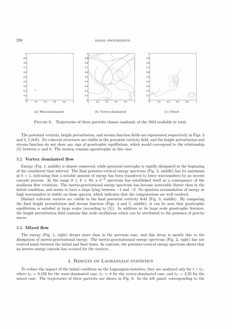
Figure 6. Trajectories of three particles chosen randomly of the 1024 available in total.

The potential vorticity, height perturbation, and stream function fields are represented respectively in Figs. 3and 4, 5 (left). No coherent structures are visible in the potential vorticity field, and the height perturbation andstream function do not show any sign of geostrophic equilibrium, which would correspond to the relationship(5) between ψ and h. The motion remains ageostrophic in this case.

3.2. Vortex dominated flow

Energy (Fig. 1, middle) is almost conserved, while potential enstrophy is rapidly dissipated at the beginningof the considered time interval. The final potentio-vortical energy spectrum (Fig. 2, middle) has its maximumat k = 1, indicating that a notable amount of energy has been transfered to lower wavenumbers by an inversecascade process. In the range 8 ≤ k ≤ 80, a k−4 spectrum has established itself as a consequence of thenonlinear flow evolution. The inertio-gravitational energy spectrum has become noticeably flatter than in theinitial condition, and seems to have a slope lying between −1 and −2. No spurious accumulation of energy athigh wavenumber is visible on these spectra, which indicates that the computations are well resolved.

Distinct coherent vortices are visible in the final potential vorticity field (Fig. 3, middle). By comparingthe final height perturbation and stream function (Figs. 4 and 5, middle), it can be seen that geostrophicequilibrium is satisfied at large scales (according to (5)). In addition to its large scale geostrophic features,the height perturbation field contains fine scale oscillations which can be attributed to the presence of gravitywaves.

3.3. Mixed flow

The energy (Fig. 1, right) decays more than in the previous case, and this decay is mostly due to thedissipation of inertio-gravitational energy. The inertio-gravitationnal energy spectrum (Fig. 2, right) has notevolved much between the initial and final times. In contrast, the potentio-vortical energy spectrum shows thatan inverse energy cascade has occured for the vortices.

4. Results on Lagrangian statistics

To reduce the impact of the initial condition on the Lagrangian statistics, they are analyzed only for t > tC ,where tC = 0.192 for the wave-dominated case, tC = 8 for the vortex-dominated case, and tC = 2.25 for themixed case. The trajectories of three particles are shown in Fig. 6. In the left panel, corresponding to the


0.1884 0.1885 0.1885 0.1885 0.1885

0.2154

0.2154

0.2154

0.2155

0.2155

0.2155

0.2155

0.2155

0.2155

(a) Wave-dominated

0.44 0.46 0.48 0.5 0.52

0.31

0.32

0.33

0.34

0.35

0.36

0.37

0.38

0.39


0.06 0.062 0.064 0.066 0.068

0.153

0.154

0.155

0.156

0.157

0.158

0.159

0.16

0.161

(c) Mixed

Figure 7. Zoom on the beginning of the trajectory of a particle, in the regions indicated bythe black square in Fig. 6. The enlargement factors are respectively 2 · 104, 20 and 200.

wave-dominated flow, the trajectories are barely visible. To enhance the tiny motion of the particle, we show azoom in Fig. 7.

The main result of this work consists in the PDFs shown in Fig. 8. In each graph, the PDFs of the firstcomponent of Lagrangian velocity and of Lagrangian acceleration are plotted along with the PDFs of the firstcomponent of Lagrangian velocity increments for varying increment size. The various PDFs have been shiftedvertically in order to better distinguish between them, with the acceleration always located at the top, thevelocity at the bottom, and the increments in the middle. The PDFs are also rescaled to have their standarddeviation equal to 1. The first thing we notice is that the PDFs of velocity increments converge to the PDFs ofLagrangian acceleration when the increments goes to zero, in agreement with (9).

For the wave-dominated flow (Fig. 8, a), all the PDFs are very nearly similar to each other, suggesting thatthe trajectories are self-similar. The PDFs are also close to being Gaussian, as indicated by the fact that theirflatness (Fig. 8, d) is nearly equal to 3. For the vortex-dominated flow (Fig. 8, b), the PDF of the Lagrangianacceleration is non Gaussian and has an inflection point around 3 standard deviations. The core of the PDF, inthe interval [−3, 3], is reminiscent ot the wave-dominated case, but the wings extend further away from zero, upto 7 standard deviations. This effect is reflected on the PDFs of Lagrangian velocity increments for ∆t ≤ 0.01.In constrast, from ∆t = 0.05 upwards, the wings take more and more importance, and the PDFs resemble thosethat were observed in incompressible 2D turbulence in [10], with values reaching 10 standard deviations. Foreven larger ∆t, as in [10], the wings lose weight again and the Lagrangian velocity PDF is closer to a Gaussian.These transitions are reflected by the behavior of the flatness (Fig. 8, d), which first raises from 7 to 30 andthen goes back down to around 7 at large increments. In the mixed case (Fig. 8, c), which contains moreinertio-gravitational energy than the wave-dominated case, the PDF of Lagrangian acceleration is very close tothe one which was observed in the wave-dominated case (Fig. 8, a). Only for time increments larger than 3.95can the effect of the vortices be detected on the PDF of velocity increments and on its flatness.

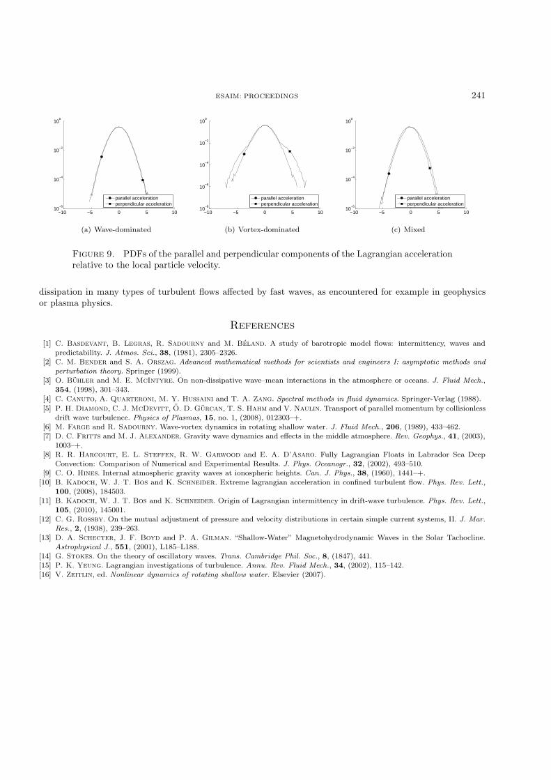
Another way of outlining the effect of the waves is to decompose the Lagrangian acceleration over the localFrenet frame attached to the particle, or in other words to project it along the directions that are parallel andorthogonal to the local Lagrangian velocity. The resulting PDFs, shown in Fig. 9, are almost overlapping in thewave-dominated and in the mixed-case, but they are markedly different in the vortex-dominated case. Moreprecisely, in the vortex-dominated case, the tails of the perpendicular acceleration PDF extend further awayfrom the origin, while the PDF of parallel acceleration remains Gaussian. This interesting effect is in fact notvery surprising, since it means that the effect of the vortices is mostly to bend the trajectories of the particles.


−10 −5 0 5 1010

−15

10−10

10−5

100

prob

abili

ty d

ensi

ty

accelerationτ = 1.27 10−6

τ = 1.01 10−5

τ = 8.05 10−5

τ = 6.44 10−4

τ = 5.15 10−3

τ = 4.12 10−2

velocity

(a) Wave-dominated

−10 −5 0 5 1010

−12

10−10

10−8

10−6

10−4

10−2

100

prob

abili

ty d

ensi

ty


τ = 2.62 10−4

τ = 2.10 10−3

τ = 1.68 10−2

τ = 1.34 10−1

τ = 1.07 100

velocity


−10 −5 0 5 1010

−15

10−10

10−5

100

prob

abili

ty d

ensi

ty


τ = 7.14 10−5

τ = 5.70 10−4

τ = 4.56 10−3

τ = 3.65 10−2

τ = 2.92 10−1

velocity

(c) Mixed

10−6

10−4

10−2

100

102

0

2

4

6

8

10

12

14

16

τ

Fla

tnes

s of

vel

ocity

incr

emen

ts

Wave−dominatedVortex−dominatedMixed

(d)

Figure 8. (a-c) PDFs of the first component of Lagrangian velocity, Lagrangian velocityincrements, and Lagrangian acceleration (see Sec. 2.2). The standard deviation is normalizedto one, and the curves have been shifted vertically for better visualization. (d) Flatness ofLagrangian velocity increments v(t+ τ) − v(t) as a function of τ for the three types of flows.

5. Conclusion

In this work, we have studied the Lagrangian statistics of rotating Saint-Venant turbulence by direct numericalsimulation, in order to shed some light on the effect fast waves can have on these quantities. We have shownthat the PDFs of Lagrangian quantities, such as velocity increments and acceleration, were strongly influenced.The extent of this influence is determined both by the amplitude of the waves and by their frequency. At leastfor short enough increments, the core of the velocity increments PDFs seems to be mostly determined by thewaves. This result could have implications on the interpretation of experimental results concerning particlesadvected by geophysical flows in the atmosphere or ocean. More generally, the Lagrangian point of view wehave proposed may help characterize the wave content of experimental or numerical flows using probes suchas drifting buoys or balloons [8]. This work is a first step towards a more comprehensive study of turbulent


−10 −5 0 5 1010

−6

10−4

10−2

100

parallel accelerationperpendicular acceleration

(a) Wave-dominated

−10 −5 0 5 1010

−8

10−6

10−4

10−2

100



−10 −5 0 5 1010

−6

10−4

10−2

100


(c) Mixed

Figure 9. PDFs of the parallel and perpendicular components of the Lagrangian accelerationrelative to the local particle velocity.

dissipation in many types of turbulent flows affected by fast waves, as encountered for example in geophysicsor plasma physics.

References

[1] C. Basdevant, B. Legras, R. Sadourny and M. Beland. A study of barotropic model flows: intermittency, waves andpredictability. J. Atmos. Sci., 38, (1981), 2305–2326.

[2] C. M. Bender and S. A. Orszag. Advanced mathematical methods for scientists and engineers I: asymptotic methods and

perturbation theory. Springer (1999).[3] O. Buhler and M. E. McIntyre. On non-dissipative wave–mean interactions in the atmosphere or oceans. J. Fluid Mech.,

354, (1998), 301–343.[4] C. Canuto, A. Quarteroni, M. Y. Hussaini and T. A. Zang. Spectral methods in fluid dynamics. Springer-Verlag (1988).

[5] P. H. Diamond, C. J. McDevitt, O. D. Gurcan, T. S. Hahm and V. Naulin. Transport of parallel momentum by collisionlessdrift wave turbulence. Physics of Plasmas, 15, no. 1, (2008), 012303–+.

[6] M. Farge and R. Sadourny. Wave-vortex dynamics in rotating shallow water. J. Fluid Mech., 206, (1989), 433–462.[7] D. C. Fritts and M. J. Alexander. Gravity wave dynamics and effects in the middle atmosphere. Rev. Geophys., 41, (2003),

1003–+.[8] R. R. Harcourt, E. L. Steffen, R. W. Garwood and E. A. D’Asaro. Fully Lagrangian Floats in Labrador Sea Deep

Convection: Comparison of Numerical and Experimental Results. J. Phys. Oceanogr., 32, (2002), 493–510.[9] C. O. Hines. Internal atmospheric gravity waves at ionospheric heights. Can. J. Phys., 38, (1960), 1441–+.

[10] B. Kadoch, W. J. T. Bos and K. Schneider. Extreme lagrangian acceleration in confined turbulent flow. Phys. Rev. Lett.,100, (2008), 184503.

[11] B. Kadoch, W. J. T. Bos and K. Schneider. Origin of Lagrangian intermittency in drift-wave turbulence. Phys. Rev. Lett.,105, (2010), 145001.

[12] C. G. Rossby. On the mutual adjustment of pressure and velocity distributions in certain simple current systems, II. J. Mar.

Res., 2, (1938), 239–263.[13] D. A. Schecter, J. F. Boyd and P. A. Gilman. “Shallow-Water” Magnetohydrodynamic Waves in the Solar Tachocline.

Astrophysical J., 551, (2001), L185–L188.[14] G. Stokes. On the theory of oscillatory waves. Trans. Cambridge Phil. Soc., 8, (1847), 441.[15] P. K. Yeung. Lagrangian investigations of turbulence. Annu. Rev. Fluid Mech., 34, (2002), 115–142.[16] V. Zeitlin, ed. Nonlinear dynamics of rotating shallow water. Elsevier (2007).

influence of waves on lagrangian acceleration in two...

Documents