INFLUENCE OF ATMOSPHERIC PRESSURE AND WATER TABLE

FLUCTUATIONS ON GAS PHASE FLOW AND TRANSPORT OF VOLATILE

ORGANIC COMPOUNDS (VOCS) IN UNSATURATED ZONES

Dissertation

by

KEHUA YOU

Submitted to the Office of Graduate Studies of Texas A&M University

in partial fulfillment of the requirements for the degree of

DOCTOR OF PHILOSOPHY

Approved by:

Chair of Committee, Hongbin Zhan

Committee Members, John R. Giardino Binayak Mohanty David W. Sparks Yuefeng Sun Head of Department, John R. Giardino

May 2013

Major Subject: Geology

Copyright 2013 Kehua You

ii

ABSTRACT

Understanding the gas phase flow and transport of volatile organic compounds

(VOCs) in unsaturated zones is indispensable to develop effective environmental

remediation strategies, to create precautions for fresh water protection, and to provide

guidance for land and water resources management. Atmospheric pressure and water

table fluctuations are two important natural processes at the upper and lower boundaries

of the unsaturated zone, respectively. However, their significance has been neglected in

previous studies. This dissertation systematically investigates their influence on the gas

phase flow and transport of VOCs in soil and ground water remediation processes using

analytically and numerically mathematical modeling.

New semi-analytical and numerical solutions are developed to calculate the

subsurface gas flow field and the gas phase transport of VOCs in active soil vapor

extraction (SVE), barometric pumping (BP) and natural attenuation taking into account

the atmospheric pressure and the water table fluctuations. The accuracy of the developed

solutions are checked by comparing with published analytical solutions under extreme

conditions, newly developed numerical solutions in COMSOL Multiphysics and field

measured data. Results indicate that both the atmospheric pressure and the tidal-induced

water table fluctuations significantly change the gas flow field in active SVE, especially

when the vertical gas permeability is small (less than 0.4 Darcy). The tidal-induced

downward moving water table increases the depth-averaged radius of influence (ROI)

for the gas pumping well. However, this downward moving water table leads to a greater

iii

vertical pore gas velocity away from the gas pumping well, which is unfavorable for

removing VOCs. The gas flow rate to/from the barometric pumping well can be

accurately calculated by our newly developed solutions in both homogeneous and multi-

layered unsaturated zones. Under natural unsaturated zone conditions, the time-averaged

advective flux of the gas phase VOCs induced by the atmospheric pressure and water

table fluctuations is one to three orders of magnitude less than the diffusive flux. The

time-averaged advective flux is comparable with the diffusive flux only when the gas-

filled porosity is very small (less than 0.05). The density-driven flux is negligible.

iv

DEDICATION

To my family

v

ACKNOWLEDGEMENTS

I would like to thank my advisor, Dr. Hongbin Zhan for his leading me into the

field of hydrogeology and guiding me through my Ph.D. Study. Dr. Zhan pays attention

not only to our education but also to our life. Dr. Zhan, thank you very much for

introducing me to numerous excellent scientists in our field, thank you very much for

your wonderful endorsement, and thank you very much for the numerous happy parties!

I would like to thank my committee members, Dr. John R. Giardino, Dr. Binayak

Mohanty, Dr. David W. Sparks, and Dr. Yuefeng Sun, for their guidance and support

throughout the course of this research. Dr. Giardino, thank you for solving my visa

problem! Dr. Mohanty, thank you for your numerous wonderful recommendation letters!

I also thank Dr. Benchun Duan a lot for the impressive recommendation letters during

my academic job application and Dr. Franco Marcantonio for serving as my committee

member in my defense.

Thanks also go to my friends and colleagues at the department of Geology &

Geophysics for their encouragement and support. I sincerely thank the financial support

from oil companies such as ConocoPhillips, Aramco and Chevron, and Berg-Hughes

Center at the department of Geology & Geophysics.

Finally, I greatly thank my husband, Dr. Xianyong Feng, for his love and help in

both my life and my Ph.D. study, and my mother, father and sisters for their persistent

encouragement and selfless love.

vi

TABLE OF CONTENTS

Page

ABSTRACT .............................................................................................................. ii

DEDICATION .......................................................................................................... iv

ACKNOWLEDGEMENTS ...................................................................................... v

TABLE OF CONTENTS .......................................................................................... vi

LIST OF FIGURES ................................................................................................... viii

LIST OF TABLES .................................................................................................... xiii

1. INTRODUCTION.............................................................................................. 1

1.1 Motivation and background ................................................................. 1 1.2 Objective .............................................................................................. 5 1.3 Organization ......................................................................................... 6

2. INFLUENCE OF ATMOSPHERIC PRESSURE AND WATER TABLE

FLUCTUATIONS ON ACTIVE SOIL VAPOR EXTRACTION ..................... 7

2.1 Introduction .......................................................................................... 7 2.2 Mathematical models ........................................................................... 8 2.3 Analysis ................................................................................................ 17 2.4 Summary and conclusions .................................................................... 44

3. BAROMETRIC PUMPING IN A HOMOGENEOUS UNSATURATED

ZONE .................................................................................................................. 48

3.1 Introduction .......................................................................................... 48 3.2 Physical and mathematical models ...................................................... 50 3.3 Analysis ................................................................................................ 66 3.4 Field application ................................................................................... 74 3.5 Summary and conclusions .................................................................... 79

4. BAROMETRIC PUMPING IN A MULTI-LAYERED UNSATURATED

vii

Page

ZONE ...................................................................................................................... 83

4.1 Introduction .......................................................................................... 83 4.2 Mathematical models ........................................................................... 83 4.3 Field application ................................................................................... 90 4.4 Summary and conclusions .................................................................... 92

5. TRANSPORT MECHANISMS OF GAS PHASE VOLATILE ORGANIC

COMPOUNDS (VOCS) IN NATURAL ATTENUATION ............................... 94

5.1 Introduction .......................................................................................... 94 5.2 Physical and mathematical models ...................................................... 97 5.3 Field application ................................................................................... 102 5.4 Analysis ................................................................................................ 108 5.5 Summary and conclusions .................................................................... 123

6. SUMMARY AND CONCLUSIONS .................................................................. 126

6.1 Summary and conclusions .................................................................... 126 6.2 Contributions ........................................................................................ 128 6.3 Future work .......................................................................................... 129

REFERENCES .......................................................................................................... 131

APPENDIX A ........................................................................................................... 143

viii

LIST OF FIGURES

FIGURE Page

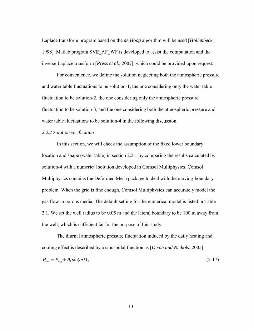
2.1 Comparison of the subsurface gas pressure calculated by solution-4 and the numerical solution at the observation point (a) r=5 m, and z=4.3 m; (b) r=10 m, and z=4.3 m; (c) r=10 m, and z=2 m; (d) r=10 m, and z=6 m. The solid lines are calculated by solution-4, and the dashed lines are calculated by the numerical solution .......................................................... 16 2.2 Comparison of the subsurface gas pressure calculated by solution-1, -2, -3 and -4 at a non-coastal site .................................................................... 19 2.3 Comparison of the subsurface gas pressure drawdown distribution with the radial distance from the well calculated by solution-1, -2, -3 and -4 at the middle depth of the well screen at 0.25 day at a non-coastal site .... 21 2.4 Comparison of the subsurface gas pressure calculated by solution-1, -2, -3 and -4 at a coastal site ............................................................................ 23 2.5 Comparison of the subsurface gas pressure drawdown distribution with the radial distance from the well calculated by solution-1, -2, -3 and -4 at the middle depth of the well screen at 0.25 day at a coastal site. ........... 24 2.6 ROIs and distributions of pore-gas velocities calculated by neglecting both atmospheric pressure and water table fluctuations (solution-1) and considering the atmospheric pressure fluctuation (solution-3) at (a) t= 0.125 day, (b) t=0.25 day, (c) t=0.5 day and (d) t=0.625 day. Solid lines are calculated by soution-1 while dashed lines are calculated by solution-3 .................................................................................................... 29 2.7 ROIs and distributions of pore-gas velocities calculated by neglecting both atmospheric pressure and water table fluctuations (solution-1) and considering the tidal-induced water table fluctuation (solution-2) at (a) t=0.05 day, (b) t=0.21 day, (c) t=0.46 day and (d) t=0.78 day. Solid lines are calculated by solution-1 while dashed lines are calculated by solution-2. .............................................................................................. 32 2.8 Comparison of the gas pressure difference between solution-3 and -1 at the observation point r=2 m, and z=4.3 m (a) with different hydrogeological parameters; (b) with different well configuration parameters .................................................................................................. 35

ix

FIGURE Page

2.9 The gas pressure contour lines and gas flow lines at 0.7 day calculated by solution-1 (a) with kr/kz=2.5; (b) with kr/kz=10; (c) with kr/kz=25; and calculated by solution-3 (d) with kr/kz=2.5; (e) with kr/kz=10; (f) with kr/kz=25 by fixing kz ..................................................................... 37 2.10 Comparison of the gas pressure difference between solution-2 and -1 at the observation points r=2 m, and z=4.3 m (a) with different hydrogeological parameters; (b) with different well configuration parameters. ................................................................................................. 41 2.11 The gas pressure contour lines and gas flow lines calculated by solution-2 at 0.7 day (a) with kr/kz=2.5; (b) with kr/kz=10; (c) with kr/kz=25 by fixing kz at coastal sites ........................................................... 43 3.1 Diagram of barometric pumping and the BPW in a homogenous unsaturated zone ......................................................................................... 51 3.2 Comparison of the total gas flow rate to/from the BPW calculated by two kinds of numerical solutions, one neglecting the gravitational effect and one considering it, and two kinds of SA solutions, one treating the well screen as a single segment and one dividing the well screen into three segments with the lengths of 0.1 m, 0.8 m, and 0.1 m, respectively. Positive values mean soil gas flows out of the unsaturated zone, while negative values mean fresh air flows into the unsaturated zone ................ 64 3.3 Comparison of subsurface gas pressure at different distance from the well calculated by the numerical solution neglecting gravitational effect (solid lines) and the SA solution treating the well screen as a single segment (dashed lines) at the depth of 33.5 m ........................................... 66 3.4 (a) Distribution of the absolute values of subsurface gas pressure deviations from the subsurface background pressure |(P*(r, z, t)-Pb(z, t))| along the radial distance from the well at different time. (b) Distribution of the absolute relative values of subsurface gas pressure deviations from the subsurface background pressure |(P*(r, z, t)-Pb(z, t))| / (P*(rw, z, t)-Pb(z, t)) along the radial distance from the well at different time ............................................................................................................. 69 3.5 Comparison of gas flow rate calculated by two SA solutions with a check valve when the well is at the depth of (a) 34.5 m and (b) 24.5 m, one using the average gas pressure as the control pressure and the other using the subsurface background gas pressure as the control pressure.

x

FIGURE Page

Positive values mean soil gas flows out of the unsaturated zone, while negative values mean fresh air flows into the unsaturated zone. ............... 73 3.6 Comparison of field measured atmospheric pressure and atmospheric pressure function obtained from Fourier series analysis, and comparison of field measured subsurface gas pressure and that calculated by the SA solution at the depth of 33.7 m ................................................................... 76 3.7 Comparison of field measured gas flow rate to/from the BPW and that calculated by two kinds of SA solutions, one treating the well screen as a single segment with a length of 0.3 m and the other treating the well screen as three segments with the lengths of 0.05 m, 0.2 m, and 0.05 m, respectively. Positive values mean soil gas flows out of the unsaturated zone, while negative values mean fresh air flows into the unsaturated zone ............................................................................................................ 79 4.1 Comparison of average gas flow velocity across the wellbore calculated by ML solution and 2-D numerical solution in a single-layered unsaturated zone ......................................................................................... 89 4.2 Subsurface gas pressure at the depth of 59.75 m calculated by the ML solution in a three-layered unsaturated zone in response to field atmospheric pressure fluctuations at the Hanford site in Richland, Washington ................................................................................................. 92 4.3 Comparison of gas flow rate calculated by the ML solution with measured flow rates in a three-layered unsaturated zone in response to field atmospheric pressure variations at the Hanford site in Richland, Washington ................................................................................................. 93 5.1 Comparisons of calculated and field measured diffusion, pressure-driven, density-driven and advective subsurface gas pressures at the depth of 2.45 m at Picatinny Arsenal in Morris County, New Jersey ...................... 104 5.2 Change of the gas phase concentration of TCE with time at (a) z=0.16 m, (b) z=1.6 m, and (c) z=3.0 m ...................................................................... 105 5.3 Calculated (a) transient diffusive and (b) advective fluxes of TCE at the depth of 0.16 m at Picatinny Arsenal in Morris County, New Jersey ........ 106 5.4 Distribution of two-day averaged (a) diffusive flux and (b) advective flux of TCE with depth at Picatinny Arsenal in Morris County, New Jersey ........ 107

xi

FIGURE Page

5.5 Comparison of diffusive, pressure-driven, density-driven and advective fluxes in the subsurface at (a) z=0.6 m; (b) z=2.4 m; (c) z=4.4 m. Positive values mean downward fluxes; negative values mean upward fluxes ......................................................................................................... 109 5.6 Comparison of ten-day averaged (a) diffusive flux, (b) pressure-driven flux, (c) density-driven flux, (d) advective flux. Positive values mean downward fluxes; negative values mean upward fluxes ........................... 111 5.7 Comparison of five-day averaged (a) diffusive fluxes and (b) advective fluxes with gas phase porosity g of 0.05, 0.2 and 0.35. Lines without markers, with circle markers and with triangle markers are fluxes with the porosity of 0.05, 0.2 and 0.35, respectively ......................................... 114 5.8 Comparison of five-day averaged (a) diffusive fluxes and (b) advective fluxes with the average water table depth H of 2.5 m, 15 m and 30 m. Solid lines with markers, solid lines without markers and dashed lines are the fluxes with the average water table depth of 2.5, 15 and 30 m, respectively. ................................................................................................ 116 5.9 Comparison of five-day averaged advective fluxes with gas phase permeability kg of 1.0×10-15 m2, 1.0×10-14 m2, 1.0×10-13 m2, 1.0×10-12 m2 and 1.0×10-11 m2. ................................................................ 117 5.10 Comparison of five-day averaged advective fluxes with the magnitude of atmospheric pressure fluctuation A1 of 100 Pa, 300 Pa, 500 Pa, 1000 Pa and 1500 Pa. ................................................................................. 118 5.11 Comparison of five-day averaged advective fluxes with the magnitude of water table fluctuation A2 of 0.001 m, 0.005 m, 0.01 m, 0.05 m and 0.1 m ........................................................................................................... 119 5.12 Comparison of five-day averaged advective and diffusive fluxes in a homogeneous and a two layered unsaturated zone. The homogeneous unsaturated zone has a gas phase saturation of 0.5; the two layered unsaturated zone has a gas phase saturation of 0.2 in the upper 1 m and 0.5 in the lower 4 m. ................................................................................... 121 5.13 Comparison of five-day averaged advective and diffusive fluxes in a homogeneous and a two layered unsaturated zone. The homogeneous

xii

FIGURE Page

unsaturated zone has a gas phase saturation of 0.5; the two layered unsaturated zone has a gas phase saturation of 0.8 in the upper 1 m and 0.5 in the lower 4 m .................................................................................... 123

xiii

LIST OF TABLES

TABLE Page

2.1 List of default input parameters, modified from Baehr and Hult [1991] ... 14

2.2 Parameter optimization results using solutions-1, -2, -3 and -4, parameters listed in Table 3.1 and hypothetical field data calculated by solution-4 .................................................................................................... 26 3.1 List of input parameters for gas flow in section 4.2.3, modified from Rossabi and Falta [2002] ........................................................................... 63 3.2 Influence of unsaturated zone properties and BPW design parameters on the range of ROI ......................................................................................... 70 4.1 List of input parameters for gas flow in a three-layered unsaturated zone 91 5.1 Default parameters (modified from Falta et al. [1989]) ............................ 112

1

1. INTRODUCTION

1.1 Motivation and background

Over the past centuries, organic compounds have been widely used in industries,

and large amounts of organic wastes are expelled carelessly into the subsurface from

leaking storage tanks, leakage of landfill sites, liquid chemical waste, wastewater

disposal lagoons and accidental release from pipelines and spillages [Rivett et al., 2011].

The European Union defines the organic compounds that have boiling points less than

250 ℃ measured at a standard atmospheric pressure of 101.3 KPa as the volatile organic

compounds (VOCs) [Rivett et al., 2011]. VOCs are one of the most pervasive

contaminants found in ground water [Cummings and Booth, 2006], and they are toxic

even when the concentrations are in several part-per-billion (ppb). Therefore, a variety

of remediation methods, such as air sparge, soil vapor extraction (SVE), amendment

application by injection or soil blending, land-farming, bioenhancement and

augmentation and groundwater pump-and-treat technology [Khan et al., 2004], have

been conducted in numerous sites around the world.

Among these remediation technologies, active SVE, where an air blower is

installed to create a vacuum to enhance the evaporation of VOCs in the unsaturated zone,

is one of the most popular techniques to remove VOCs [Khan et al., 2004]. It has been

used at 20% of all Superfund sites [EPA, 1997]. It is even more common at non-

Superfund sites [Jennings and Patil, 2002]. Active SVE not only promises good results

2

in short time, but also is cost-effective, technology-simple, and has least disturbance to

remediation sites [Frank and Barkley, 1995; Khan et al., 2004]. However, a recent

survey of 59 sites contaminated by chlorinated solvents were not able to achieve the

maximum contaminant levels allowed after one to five years’ operation of active source

treatment technologies [Kamath et al., 2009]. The concentration of these remaining

VOCs are mainly decreased by barometric pumping (BP) and natural attenuation

processes including biodegradation, dispersion, dilution, sorption, volatilization,

chemical or biological stabilization, transformation, etc. [Choi and Smith, 2005].

When an open well is installed in an unsaturated zone, gas can flow between the

subsurface and the well depending on the gas pressure gradient near the well. This

process is named BP (which is also called passive SVE) and the well is called barometric

pumping well (BPW) [Rossabi et al., 1993; Rohay et al., 1993; Jennings and Patil, 2002;

Riha, 2005]. The BPW exhales the VOCs out of the soil and inhales the fresh air into the

soil without mechanical pumping, thus is a favored passive remediation technology in

the unsaturated zone [Ellerd et al., 1999; Rossabi and Falta, 2002; Neeper, 2003;

Rossabi, 2006]. It is especially applicable to sites where the gas pumping efficiency is

mass-transfer controlled [Rohay et al., 1993; Ellerd et al., 1999; Rossabi and Falta,

2002; Riha, 2005], or where the rapid removal of VOCs is not required [Murdoch, 2000].

Since 1990, it has been applied in hundreds of sites in the United States to remediate

VOCs either as a stand-alone measure or in conjunction with active SVE [Kamath et al.,

2009; Murdoch, 2000]. Enhancement techniques such as a low permeable surface seal

3

and a one-way check valve can be installed to improve the mass removal efficiency in

the field BP [Ellerd et al., 1999].

The atmospheric pressure on the ground surface and the water table serve as the

upper Dirichlet type and lower variable flux type boundary conditions for the gas flow

and mass transport in the unsaturated zone. In BP, the driving force is the atmospheric

pressure fluctuation.

Generally, there are two types of atmospheric pressure fluctuation. One is the

diurnal change induced by solar/terrestrial heating and cooling effects. This diurnal

atmospheric pressure fluctuation has been described by a sinusoidal function [Neeper,

2003]. The other is the irregular transit of a cold or warm front, which can cause

atmospheric pressure to change as intensively as 20 mbar to 30 mbar within 24 hours

[Massmann and Farrier, 1992]. This type of atmospheric pressure fluctuation is

sometimes described by a first order linear function.

Water table fluctuation could be induced by seasonal variations of precipitation,

melt-frozen effect, evapotranspiration, cyclic pumping of near-by wells, stream stage

change, earthquake, land usage, climate change, ocean tides, etc. [Turk, 1975]. The

increase of temperature decreases surface tension and expands air volume entrapped in

capillary pores, drives water down to the phreatic surface, and increases water level, and

vice versa [Turk, 1975]. This effect lags in time depending on the depth to the water

table. The diurnal barometric cycles resulting from the solar heating/cooling effect can

also cause the contraction or expansion of air volume in the capillary fringe and the

fluctuation of the water level in a shallow aquifer [Turk, 1975]. Turk [1975] found that

4

the water table varied daily up to 1.5-6 cm in summer and 0.5-1.0 cm in winter, the

highest one occurred in the late afternoon and the lowest in the middle morning in a

shallow aquifer at the Bonneville Salt Flats, Utah. Besides, the water level is found to

change with plant water usage, which is controlled daily by the global irradiance and

seasonally by the global irradiance and temperature. However, if the primary source of

plant water is the unsaturated zone, water table fluctuation will be greatly diminished

[Butler et al., 2007]. At a non-coastal site, water level does not necessarily fluctuate in a

given aquifer setting (for example, a deep water table), and the fluctuations are usually

limited to a few centimeters in amplitude. However, at a coastal site, water table

fluctuates regularly with the diurnal and semi-diurnal tidal effects [Nielsen, 1990;

Raubenheimer, 1999].

Atmospheric pressure and water table fluctuations usually have less influence on

the subsurface gas pressure change and the mass transport compared with that induced

by well extractions or injections. However, the pressure fluctuation could significantly

increase the rate of vapor-phase contaminant transport in fractured media and can be an

important mechanism for driving vapor-phase contaminant out of the unsaturated zone

without active pumping [Nilson et al., 1991; Pirkle et al., 1992; Auer, 1996]. Dixon and

Nichols [2005] suggested that when interpreting data from the unsaturated zone gas

pumping test, atmospheric pressure fluctuation should be carefully examined.

The high-frequency, and often high-amplitude water table fluctuation at a coastal

site plays an important role in gas flow in the unsaturated zone. It causes the dome-

shaped heave features in the extensively paved coastal areas of Hong Kong [Jiao and Li,

5

2004; Li and Jiao, 2005]. The increase of the magnitude and frequency of the water table

fluctuation could nonlinearly increase the advective flux of volatile organic compounds

(VOCs) in the subsurface [Choi and Smith, 2005].

However, for the convenience of mathematical treatment, the atmospheric

pressure and the water table position are always assumed to be fixed and independent of

time [Baehr and Hult, 1991; Baehr and Joss, 1995; Falta, 1995]. Now the questions are:

can we neglect the effects of atmospheric pressure and water table fluctuations when

dealing with actively induced gas flow in the unsaturated zone? If the answer is yes,

under what constrains? How can we quantify the gas flow rate induced by the

atmospheric pressure fluctuation? Will the pressure-driven flux induced by the

atmospheric pressure and water table fluctuations dominate the gas phase transport of

VOCs in the unsaturated zone?

1.2 Objective

The objective of this study is to investigate the influence of the atmospheric

pressure and water table fluctuations on the gas phase flow and transport of VOCs in the

subsurface using process-based mathematical models. Specifically, this study focuses on

the following goals:

1. Study the influence of atmospheric pressure and water table fluctuations on the

subsurface gas flow field in active SVE at both coastal and non-coastal sites.

2. Investigate the gas flow field in BP and quantify the gas flow rate to/from the

BPW in both homogeneous and multi-layered unsaturated zones.

6

3. Explore the relative significance of the gas phase transport mechanisms of

VOCs in unsaturated zones under various natural conditions.

1.3 Organization

This dissertation is organized as follows: in section 2, the influence of

atmospheric pressure and water table fluctuations on active SVE is explored at both

coastal and non-coastal sites, and suggestions are provided to accurately interpret the

actively induced gas flow data measured in the field; in section 3, new semi-analytical

solutions are developed to calculate the subsurface flow field and gas flow rate to/from

the BPW with and without check valves installed in a homogeneous unsaturated zones,

and methods are provided to estimate ROIs in BP; in section 4, the model for gas flow in

BP is extended to a multi-layered unsaturated zone, and the developed solution is

applied to interpret the field BP at the Savannah River Site in Aiken, South Carolina; in

section 5, a comprehensive study using the finite difference numerical method is

conducted to explore the relative significance of the diffusive flux, pressure-driven

advective flux and density-driven advective flux of gas phase VOCs in natural

attenuation under various geoenvironmental conditions; this dissertation is ended with a

brief summary and several conclusions in section 6.

7

2. INFLUENCE OF ATMOSPHERIC PRESSURE AND WATER TABLE

FLUCTUATIONS ON ACTIVE SOIL VAPOR EXTRACTION*

2.1 Introduction

Gas flow in the unsaturated zone is a very important research subject in many

disciplines including hydrology, soil science, environmental engineering, geotechnical

engineering, etc. [Rossabi and Falta, 2002]. The atmospheric pressure on the ground

surface and the water table serve as the upper Dirichlet type and lower variable flux type

boundary conditions for such a gas flow problem. Traditionally, for the convenience of

mathematical treatment, these two boundary conditions are assumed to be fixed and

independent of time [Baehr and Hult, 1991; Cho and Diguilio, 1992; Shan et al., 1992;

Baehr and Ross, 1995; Falta, 1995; Ge and Liao, 1996; Ge, 1998; DiGiulio and

Varadhan, 2001; Zhan and Park, 2002; Dixon and Nichols, 2006; Switzer and Kosson,

2007]. In reality, gas flow in the unsaturated zone will inevitably be affected by

atmospheric pressure fluctuations on the ground surface. In addition to this, it will be

affected by water table fluctuations, particularly when the unsaturated zone is close to an

ocean where the daily tide may induce considerable water table fluctuations. Now the

question is: can we neglect the effects of atmospheric pressure and water table

fluctuations when dealing with actively induced gas flow in the unsaturated zone? If the

answer is yes, under what constrains? The purpose of this study is to build a theoretical

*Reprinted with permission from "Can atmospheric pressure and water table fluctuations be neglected in soil vapor extraction" by You, K., and H. Zhan (2012), Adv. Water

Resour., 35, 41-54, Copyright [2012] by Elsevier.

8

basis or evaluation criterion for determining if atmospheric pressure and water table

fluctuations can be neglected in SVE models. A new two-dimensional (2-D) semi-

analytical solution taking into account the atmospheric pressure and water table

fluctuations in SVE will be developed. ROIs and subsurface gas pressure will be

analyzed and compared to answer the questions above. One should note that the

parameters and equations defined in section 2 only apply to section 2.

2.2 Mathematical models

2.2.1 Development of the new solution

The coordinate system for 2-D gas flow in SVE in an unsaturated zone is set as

follows. The origin of the coordinate system is set at the ground surface. The z axis is

vertical, positive downward and through the axis of the gas injection/extraction well,

where gas flows at a rate of Q (L3T-1) and Q is positive for injection. The r axis is

horizontally radial. The unsaturated zone is open to the atmosphere, and has a thickness

of h (L). The gas injection/extraction well is screened from the depth of a to b (L).

Assuming the unsaturated zone to be homogenous but vertically anisotropic, the

linearized governing equation for the transient gas flow is [Baehr and Hult, 1991; Falta,

1995; You et al., 2011b]:

2

222

2

222

avg z

Pk

r

P

r

k

r

Pk

t

P

P

nSz

rr

gg

, (2-1)

where t is time (T); P is the subsurface gas pressure (ML-1T-2); Pavg is the average gas

pressure (ML-1T-2); kr, kz are the radial and vertical gas permeabilities (L2), respectively;

9

n is the porosity (dimensionless); Sg is the volumetric gas-phase saturation

(dimensionless); g is the gas dynamic viscosity (ML-1T-1).

The radial and vertical gas permeabilities kr and kz are dependent on soil moisture,

which could be redistributed by water movement induced by gas injection or extraction

through the well in SVE [Baehr and Hult, 1991]. Therefore, kr and kz vary with space

and time, which complicates the problem greatly. In order to obtain a simple semi-

analytical solution, we neglect the heterogeneity of kr and kz in this study as in previous

studies, such as Baehr and Hult [1991].

When the fluctuation of the atmospheric pressure is taken into account, the gas

pressure at the upper boundary should be altered from the common treatment of a

constant average pressure to the time-dependent atmospheric pressure Patm(t), that is,

0),(2atm

2 ztPP . (2-2)

When the fluctuation of the water table is taken into account, the lower boundary

condition should be altered from the common treatment of no-flux boundary to

hzk

tvnSP

z

P

z

gg

hz

,

)(2| wtavg

2 , (2-3)

where vwt(t) is the velocity of the water table movement (LT-1). Eq. (2-3) is derived by

applying Darcy’s law to the water table to calculate the water table movement velocity

from the pressure gradient. This same treatment is employed in Choi and Smith [2005].

One should note that in Eq. (2-3), the depth of the water table is fixed to be h, and the

shape of the water table is assumed to be horizontal. However, the depth and the shape

10

of the water table or the unsaturated zone thickness actually fluctuate. The error induced

by this assumption will be checked in section 2.2.2.

The well casing is a no-flux boundary, while the well screen is a fixed-flux

boundary, which are described by

limr ¶P2

¶rr®0

= 0, 0 < z < b,a < z < h, (2-4a)

*2

0

lim ,( )

g

rr

QPPr b z a

r k a b

, (2-4b)

where P* is the gas pressure where Q is measured (ML-1T-2). Q is usually assumed to be

a constant value and positive for gas injection [Falta, 1995]. In field operations, Q can

be easily measured by flow meters [Baehr and Hult, 1991].

The lateral boundary is infinitely far from the well, thus will not affect gas flow

to/from the well [You et al., 2011b]. We arbitrarily choose a fixed-pressure boundary at

the lateral infinity [You et al., 2011b]. Therefore,

P2 = Pavg2 , r®¥ . (2-5)

Increasing the initial subsurface gas pressure would increase the average value of

the subsurface gas pressure the same amount as that of the initial one uniformly across

the unsaturated zone at steady state, and vice versa. For convenience, the initial

subsurface gas pressure is assumed to be uniform and equals the average gas pressure

[You et al., 2011b]. Thus, one has

P2(t = 0,r, z) = Pavg2 . (2-6)

11

For simplicity, we use the following parameters to transform Eqs. (2-1)-(2-6) into

dimensionless ones:

.)(

,,2

,,,,,,

2avg

*

2avg

2avg

2atm

wtavg

wt

2avg

2avg

2

2avg

Pbak

QPQ

P

PPfv

kP

hnSv

P

PP

h

bb

h

aa

h

zz

k

k

h

rrt

nSh

Pkt

r

g

DD

z

gg

D

DDDD

r

zD

gg

z

D

(2-7)

Substituting Eq. (2-7) into Eqs. (2-1)-(2-6), one has

2

2

2

2 1

D

D

D

D

DD

D

D

D

zrrrt

, (2-8)

0),,0( DDDD zrt , (2-9)

0, DDD zf , (2-10)

Dz

D

D vz D wt1|

, (2-11)

1,0,0lim0

DDDD

D

DD

rzabz

rr

D

, (2-12a)

DDDD

D

DD

razbQ

rr

D

,lim

0

, (2-12b)

DD r,0 . (2-13)

Successively applying the Laplace transform to tD and finite Fourier transform to

zD in Eqs. (2-8)-(2-13), one could obtain the solution to Eqs. (2-8)-(2-13) in the Laplace

domain (The detailed derivation process is shown in the Appendix A):

)sin()1()()]cos()[cos(21

2wt

1

22

0 Dn

n n

D

n

n

DnDnDnDn

n

DD zd

sd

v

sd

fdrsdKbdad

d

Q

,

(2-14)

12

where s is the dimensionless Laplace transform factor; over bar means the parameters in

Laplace domain; )5.0( ndn ; n are positive integers; K0 is the second-kind, zero-

order modified Bessel function.

Compared with the common case of fixed gas pressure at the ground surface and

zero gas flux at the water table, Eq. (2-14) has two additional terms, the term

sd

fd

n

Dn

2 accounting for the atmospheric pressure fluctuation, and the term

sd

v

n

D

n

2wt

1)1( accounting for the water table fluctuation. If both terms are neglected, one

has

)sin()()]cos()[cos(21

20 Dn

n

DnDnDn

n

DD zdrsdKbdad

d

Q

. (2-15)

Applying the analytical inverse Laplace transform to Eq. (2-15), one obtains

)sin(),4

()]cos()[cos(1

2

Dn

n

nD

D

DDnDn

n

DD zddr

t

rWbdad

d

Q

, (2-16)

where ),( vuW is the leaky well function [Hantush, 1964] defined as

dyy

vy

yvuW

u)

4exp(1),(

2

. Eq. (2-16) describes the subsurface gas pressure

distribution in SVE neglecting both the atmospheric pressure and water table

fluctuations. Eq. (2-16) has the same form as that in Eqs. (9)-(12) in Falta [1995], which

demonstrates the validity of the new solution in Eq. (2-14).

If the expressions for Df and D

vwt in Eq. (2-14) are complicated, it is not easy to

obtain a simple closed-form solution in real-time domain; instead, a numerical inverse

13

Laplace transform program based on the de Hoog algorithm will be used [Hollenbeck,

1998]. Matlab program SVE_AF_WF is developed to assist the computation and the

inverse Laplace transform [Press et al., 2007], which could be provided upon request.

For convenience, we define the solution neglecting both the atmospheric pressure

and water table fluctuations to be solution-1, the one considering only the water table

fluctuation to be solution-2, the one considering only the atmospheric pressure

fluctuation to be solution-3, and the one considering both the atmospheric pressure and

water table fluctuations to be solution-4 in the following discussion.

2.2.2 Solution verification

In this section, we will check the assumption of the fixed lower boundary

location and shape (water table) in section 2.2.1 by comparing the results calculated by

solution-4 with a numerical solution developed in Comsol Multiphysics. Comsol

Multiphysics contains the Deformed Mesh package to deal with the moving-boundary

problem. When the grid is fine enough, Comsol Multiphysics can accurately model the

gas flow in porous media. The default setting for the numerical model is listed in Table

2.1. We set the well radius to be 0.05 m and the lateral boundary to be 100 m away from

the well, which is sufficient far for the purpose of this study.

The diurnal atmospheric pressure fluctuation induced by the daily heating and

cooling effect is described by a sinusoidal function as [Dixon and Nichols, 2005]

)sin( 11avgatm tAPP , (2-17)

14

Table 2.1 List of default input parameters, modified from Baehr and Hult [1991]. Parameter descriptions Values Horizontal permeability (kr), Darcy 10 Vertical permeability (kz), Darcy 4 Gas-filled porosity (ng) 0.2 Air dynamic viscosity( g ), kgm-1sec-1 1.73×10-5 Depth of the lower end of well screen (a), m 4.6 Depth of the upper end of well screen (b), m 4.0 Depth of water table (h), m 8.0 Gas pumping rate (Q), m3sec-1 -0.02 Average gas pressure (Pavg), Pa 105

where A1 is the amplitude of the atmospheric pressure fluctuation (ML-1T-2), and we set

A1=150 Pa; 1 is the frequency of the diurnal atmospheric pressure fluctuation (T-1), and

86400/21 sec-1.

In a non-coastal site, barometric cycles could induce the diurnal water table

fluctuation in a shallow aquifer. Because both the lowest water table depth (or highest

water level) and the atmospheric pressure usually occur in the late afternoon [Chapman

and Lindzen, 1970; Turk, 1975], the phase difference between the atmospheric pressure

and water table depth cycles is set to be 0. Thus, the depth of the diurnal water table

fluctuation in a non-coastal site is described by

)sin( 22 tAhH , (2-18)

where H is the time-dependent water table depth (L); A2 is the amplitude of the water

table fluctuation (L) in a shallow aquifer with a value of 0.02 m in a non-coastal site;

2 is the frequency of the water table fluctuation (T-1), and 86400/22 sec-1. The

time derivative of H is the velocity of water table movement. Therefore, one has

15

)cos( 222wt tAdt

dHv . (2-19)

The diurnal atmospheric pressure fluctuation described in Eq. (2-17) and the

diurnal water table fluctuation described in Eqs. (2-18) and (2-19) are employed as the

upper and lower boundary conditions, respectively. The magnitude of the atmospheric

pressure fluctuation is set to be 150 Pa. The magnitude of the diurnal water table

fluctuation is deliberately set to be 0.5 m, which is much larger than the value of 0.02 m

in a non-coastal site. Therefore, if the error induced from this large magnitude water

table fluctuation compared to the time-averaged subsurface gas pressure is acceptable, it

will be safe to describe a small magnitude water table fluctuation boundary condition as

in Eq. (2-3), because the time-averaged subsurface gas pressure is mainly controlled by

the gas pumping rate rather than the water table fluctuation (This can be detected in

section 2.3.1).

Fig. 2.1 shows the comparison of the subsurface gas pressure calculated by

solution-4 and the numerical solution at the observation points of r=5 m and z=4.3 m

(Fig. 2.1a), r=10 m and z=4.3 m (Fig. 2.1b), r=10 m and z=2 m (Fig. 2.1c), and r=10 m

and z=6 m (Fig. 2.1d). The solid lines in Fig. 2.1 stand for the results of solution-4, and

the dashed lines stand for the results of the numerical solution. One may notice that the

observation points in Fig. 2.1 are all relatively far from the gas pumping well. The

reason is that the numerical solution in Comsol Multiphysics has to use the gas pressure

P as the dependent variable, while solution-4 uses the squared gas pressure P2 as the

dependent variable. The difference of the subsurface gas pressure calculated using P

16

0 2 4 6 8

x 104

9.9

9.92

9.94

9.96x 10

4

gas p

ressu

re (

Pa)

0 2 4 6 8

x 104

9.96

9.98

10x 10

4

0 2 4 6 8

x 104

9.97

9.98

9.99

10

x 104

time (sec)

0 2 4 6 8

x 104

9.94

9.96

9.98

10x 10

4

(a)

(c)

(b)

(d)

Figure 2.1 Comparison of the subsurface gas pressure calculated by solution-4 and the numerical solution at the observation point (a) r=5 m, and z=4.3 m; (b) r=10 m, and z=4.3 m; (c) r=10 m, and z=2 m; (d) r=10 m, and z=6 m. The solid lines are calculated by solution-4, and the dashed lines are calculated by the numerical solution.

P2 as the dependent variables is small when the gas pressure vacuum is small; and the

gas pressure vacuum decreases with the distance from the gas pumping well. Therefore,

in order to minimize the gas pressure difference caused by these two different dependent

variables, we chose the observation points to be relatively far from the well.

In order to check the discrepancy between the calculated subsurface gas

pressures using P and P2 as the dependent variables, we first fixed the water table

position in both solution-4 and the numerical solution and compared results. We find

that when the radial distance from the well r is no smaller than 5 m, the discrepancy

between the calculated subsurface gas pressures using P and P2 as the dependent

17

variables is undetectable. Therefore, the differences observed in Fig. 2.1 are expected to

be caused by the different treatment of the water table position, which is fixed in

solution-4 but fluctuated in the numerical solution. Fig. 2.1 indicates that the differences

between the subsurface gas pressures calculated by solution-4 and the numerical solution

are all less than 0.1% of the average subsurface gas pressure. Water table fluctuation is

expected to have greater impact on vertical rather than horizontal gas flows; i.e., its

influence is supposed to be more sensitive to the change of z rather than r. Therefore, the

conclusion drawn from Fig. 2.1 is expected to hold for points with other r values. In

summary, the assumption of a fixed lower boundary location used in Eq. (2-3) is

acceptable for the purpose of this study.

2.3 Analysis

2.3.1 Subsurface gas pressure distribution

In this section, solution-1, -2, -3 and -4 were compared to check the accuracy of

the previous studies neglecting both the atmospheric pressure and water table

fluctuations in SVE. Comparisons were divided into coastal and non-coastal sites,

because the water table behaves quite differently at coastal and non-coastal sites. For

both cases, the diurnal atmospheric pressure fluctuation induced by the daily solar

heating and cooling effect described in Eq. (2-17) is used as the input atmospheric

pressure. In a non-coastal site, the diurnal water table fluctuation induced by barometric

cycles or temperature changes in a shallow aquifer described in Eqs. (2-18) and (2-19) is

used to calculate the water table velocity.

18

In a coastal site, the water table fluctuation induced by diurnal and semi-diurnal

tidal effects is described by [Li and Jiao, 2005; Li et al., 2011]

3 3 3 4 4 4cos( ) cos( )H h A t c A t c , (2-20)

where A3 and A4 are the magnitudes (L) of the diurnal and semi-diurnal water table

fluctuations, respectively, and they are usually in tens of centimeters scales; 3 and

4 are the frequencies (T-1) of the diurnal and semi-diurnal water table fluctuations,

respectively. According to Li and Jiao [2005] and Li et al. [2011], one has A3=0.61 m,

A4=0.47 m, 86400/23 sec-1, 43200/24 sec-1, c3 =1.01rad , and c4 = 0.93 rad .

Therefore, the water table velocity is

wt 3 3 3 3 4 4 4 4sin( ) sin( )dHv A t c A t c

dt . (2-21)

The other default parameters are listed in Table 2.1. Fig. 2.2 shows the

comparison of the subsurface gas pressure calculated by solution-1, -2, -3 and -4 at the

observation point r=2 m, and z=4.3 m at a non-coastal site. This observation point is at

the middle depth of the well screen, which is a typical location where the gas pressure is

employed to characterize the unsaturated zone. Hence, accurate simulation of the gas

pressure there is important. According to Fig. 2.2, the computed gas pressure by

solution-1 and -2 are quite similar. The gas pressure at the observation point decreases

quickly once gas pumping starts, and reaches steady state in about 20 minutes. The

difference between solution-1 and -2 is that solution-2 takes into account the water table

fluctuation, while solution-1 does not. Therefore, their similar results indicate that the

magnitude of the daily water table fluctuation in centimeters scale in a non-coastal site is

19

too small to induce detectable influence on the subsurface gas pressure distribution in

SVE.

0 1 2 3 4 5 6 7 8

x 104

9.78

9.8

9.82

9.84

9.86

9.88

9.9

9.92x 10

4

time (sec)

gas p

ressu

re (

Pa)

solution-1

solution-2

solution-3

solution-4

Figure 2.2 Comparison of the subsurface gas pressure calculated by solution-1, -2, -3 and -4 at a non-coastal site.

When the atmospheric pressure fluctuation is considered, the subsurface gas

pressure never reaches steady state, as is evident in solution-3 and -4. Instead, the

subsurface gas pressure fluctuates around an average. When the atmospheric pressure is

higher than the average gas pressure, the subsurface gas pressure is higher than its

average value as well, and vice versa. The magnitude of the subsurface gas pressure

fluctuation is about 150 Pa, which is the same as that of the atmospheric pressure

fluctuation. Their phase difference is also negligible. That is because the depth of the

20

observation point is shallow and the retardation of the unsaturated zone to the

atmospheric pressure wave is quite small. The similarity between the results computed

by solution-3 and -4 further demonstrates that the water table effect is negligible on the

subsurface gas pressure distribution in SVE.

Fig. 2.3 shows the spatial distribution of the subsurface gas pressure drawdown

calculated by solution-1, -2, -3 and -4 at the depth of 4.3 m at a non-coastal site at 0.25

day, when the atmospheric pressure is highest, and the water level is lowest during their

one-day cycles. In Fig. 2.3, the initial subsurface gas pressure is set as the base value.

According to Fig. 2.3, the spatial distribution of the subsurface gas pressure drawdown

calculated by solution-1 and -2 are undistinguishable, and that calculated by solution-3

and -4 are undistinguishable as well. The pressure drawdown including the atmospheric

pressure effect (solution-3 and -4) is smaller than that neglecting its effect (solution-1

and -2) by a value of about 150 Pa across the entire radial distance at the middle depth of

the well screen (4.3 m). That is because the atmospheric pressure fluctuation mainly

impact the vertical gas flow, and the 4 Darcy vertical gas permeability is large enough

that cannot induce detectable attenuation to the atmospheric pressure wave at the depth

of 4.3 m. Therefore, the water table effect could be neglected, while the atmospheric

pressure effect should be taken into account for a rigorous interpretation of SVE data if

the initial subsurface gas pressure is used as the base value. Because the closer to the

well, the greater the influence from the gas pumping well and relatively less influence

from the atmospheric pressure, field gas pressure drawdown data from the observation

points close to the well are recommended to be used.

21

1 2 3 4 5 6 7 8 9 100

500

1000

1500

2000

2500

3000

3500

4000

4500

r (m)

gas p

ressu

re d

raw

do

wn

(P

a)

solution-1

solution-2

solution-3

solution-4

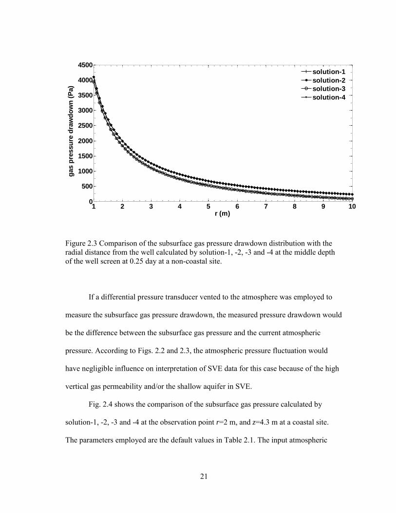
Figure 2.3 Comparison of the subsurface gas pressure drawdown distribution with the radial distance from the well calculated by solution-1, -2, -3 and -4 at the middle depth of the well screen at 0.25 day at a non-coastal site.

If a differential pressure transducer vented to the atmosphere was employed to

measure the subsurface gas pressure drawdown, the measured pressure drawdown would

be the difference between the subsurface gas pressure and the current atmospheric

pressure. According to Figs. 2.2 and 2.3, the atmospheric pressure fluctuation would

have negligible influence on interpretation of SVE data for this case because of the high

vertical gas permeability and/or the shallow aquifer in SVE.

Fig. 2.4 shows the comparison of the subsurface gas pressure calculated by

solution-1, -2, -3 and -4 at the observation point r=2 m, and z=4.3 m at a coastal site.

The parameters employed are the default values in Table 2.1. The input atmospheric

22

pressure fluctuation is described by Eq. (2-17), and the input water table velocity is

described by Eq. (2-21). According to Fig. 2.4, the subsurface gas pressure does not

reach steady state when either the atmospheric pressure or water table fluctuation is

included at a coastal site. However, unlike the non-coastal site, the water table undulates

the subsurface gas pressure greatly at a coastal site. That is because the magnitudes of

the tidal-induced water table fluctuation are much greater than those at a non-coastal site.

When the water table moves upward, the subsurface gas pressure increases to above its

average value because of the compressing effect. However, one should note that because

of the large storage capacity of water-table aquifers, ocean-driven tidal effects attenuate

within a distance of hundreds of meters from shore.

When both the effects of atmospheric pressure and water table are considered in

SVE, the discrepancies between solutions considering and neglecting their effects are

amplified when the atmospheric pressure is increasing and the water table is moving

upward simultaneously, or when the atmospheric pressure is decreasing and the water

table is moving downward simultaneously (Fig. 2.4). The discrepancies are mitigated at

other time because of their contrary effects on subsurface gas pressure behaviors (Fig.

2.4).

23

0 1 2 3 4 5 6 7 8

x 104

9.76

9.78

9.8

9.82

9.84

9.86

9.88

9.9

9.92x 10

4

time (sec)

gas p

ressu

re (

Pa)

solution-1

solution-2

solution-3

solution-4

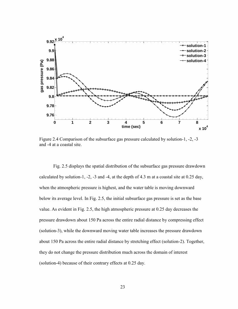
Figure 2.4 Comparison of the subsurface gas pressure calculated by solution-1, -2, -3 and -4 at a coastal site.

Fig. 2.5 displays the spatial distribution of the subsurface gas pressure drawdown

calculated by solution-1, -2, -3 and -4, at the depth of 4.3 m at a coastal site at 0.25 day,

when the atmospheric pressure is highest, and the water table is moving downward

below its average level. In Fig. 2.5, the initial subsurface gas pressure is set as the base

value. As evident in Fig. 2.5, the high atmospheric pressure at 0.25 day decreases the

pressure drawdown about 150 Pa across the entire radial distance by compressing effect

(solution-3), while the downward moving water table increases the pressure drawdown

about 150 Pa across the entire radial distance by stretching effect (solution-2). Together,

they do not change the pressure distribution much across the domain of interest

(solution-4) because of their contrary effects at 0.25 day.

24

1 2 3 4 5 6 7 8 9 100

500

1000

1500

2000

2500

3000

3500

4000

4500

r (m)

gas p

ressu

re d

raw

do

wn

(P

a)

solution-1

solution-2

solution-3

solution-4

Figure 2.5 Comparison of the subsurface gas pressure drawdown distribution with the radial distance from the well calculated by solution-1, -2, -3 and -4 at the middle depth of the well screen at 0.25 day at a coastal site.

In order to further explore the influence of the atmospheric pressure and water

table fluctuations on SVE data interpretation, we set the subsurface gas pressure

drawdown from the current atmospheric pressure (i.e., a differential pressure transducer

is used) at observation point r=2 m, and z=4.3 m calculated by solution-4 with the

parameters listed in Table 2.1 as the hypothetical field data at both coastal and non-

coastal sites. After that, we did parameter optimization using solutions-1, -2, -3 and -4 to

search for the vertical and horizontal gas permeability. The results of this study should

not be sensitive to the radial coordinates of the observation point, because as seen in Figs.

2.3 and 2.5, the discrepancies among different solutions are not sensitive with the radial

distance from the well. We set the observation point at the middle depth of the well

screen, because as we discussed previously field gas pressure drawdown data from the

25

observation points close to the well are recommended to be used. Simplex method is

employed in parameter optimization because of its simplicity and fast convergence.

Parameter optimization by solution-4 is used to check the accuracy of the parameter

optimization method. The results are listed in Table 2.2. According to Table 2.2, this

parameter optimization method is accurate enough for the purpose of this study, as

demonstrated by the exact calculated results and the small RMSE ( kr =10.00Darcy,

kz = 4.00Darcy for both sites; RMSEs are both around 133 10 Pa). At both coastal and

non-coastal sites, results calculated by both solutions-2 and -3 are quite different from

the hypothetical field values (Table 2.2). Results calculated by solution-1 are relatively

closer to the hypothetical field values ( kr =10.00Darcy, kz = 4.00Darcy at a non-coastal

site, and kr = 9.63Darcy, kz = 4.12Darcy at a coastal site). However, solution-1 has a

large REMS (108 Pa), which means solution-1 poorly predicts the subsurface gas

pressure. Although the horizontal and vertical gas permeabilities estimated by solution-3

at non-coastal sites are different from the hypothetical field values, solution-3 can

accurately predict the subsurface gas pressure (REMS for solution-3 is only 4 Pa). At a

non-coastal site, solutions neglecting the atmospheric pressure fluctuation (solutions-1

and -2) have the largest RMSE (around 108 Pa); while at a coastal site, solutions

neglecting the water table fluctuation (solutions-1 and -3) have the largest RMSE (267 Pa

and 215 Pa respectively).

26

Table 2.2 Parameter optimization results using solutions-1, -2, -3 and -4, parameters listed in Table 2.1 and hypothetical field data calculated by solution-4. kr (Darcy) kz (Darcy) REMS (Pa) Non-coastal site:

Solution-1 10.00 4.00 108 Solution-2 9.31 4.24 108 Solution-3 10.80 3.74 4 Solution-4 10.00 4.00 133 10

Coastal site: Solution-1 9.63 4.12 267 Solution-2 11.7 3.49 103 Solution-3 7.14 5.25 215 Solution-4 10.00 4.00 133 10

Note: Solution-1 neglects both the atmospheric pressure and water table fluctuations; solution-2 considers only the water table fluctuation; solution-3 considers only the atmospheric pressure fluctuation; solution-4 considers both the atmospheric pressure and water table fluctuations.

In summary, in a non-coastal site where the daily water table fluctuation is in

centimeters scale, the water table effect is negligible but the atmospheric pressure effect

should be taken into account for the interpretation of gas pressure data. In a coastal site

where the daily water table fluctuation is in tens of centimeters scale, both the water

table and atmospheric pressure fluctuations need to be considered, and the errors induced

from neglecting their effects are amplified when the atmospheric pressure is increasing

and the water table is moving upward simultaneously, or when the atmospheric pressure

is decreasing and the water table is moving downward simultaneously.

2.3.2 Radius of influence (ROI)

ROI is one of the most important parameters in the design of a SVE system. As

27

defined by the US Environmental Protection Agency (EPA), ROI is the greatest distance

from an extraction well at which a sufficient vacuum and vapor flow can be induced to

adequately enhance the volatilization and extraction of the contaminants in the

unsaturated zone [US EPA, 1994]. Extraction wells should be placed so that the overlap

in their ROIs completely covers the area of contamination [US EPA, 1994; You et al.,

2010]. In order to efficiently remove contaminants from the unsaturated zone, DiGuilio

and Varadhan [2001] used a critical pore-gas velocity (It is defined as the pore-gas

velocity that results in slight deviation from equilibrium conditions) of 0.01 cm/s to

determine the ROI for a gas pumping well.

The vertical pore-gas velocity Vz (LT-1) and radial pore-gas velocity Vr (LT-1) in

SVE are calculated by

D

D

gg

z

gg

zz

zPh

P

n

k

z

P

n

kV

2

2avg , (2-22)

2avg

2r zr D

r

g g g g D

Pk kk PV

n r n Ph r

, (2-23)

where DD z and DD r can be obtained by applying numerical inverse Laplace

transform to DD z and D Dr , respectively. DD z and

D Dr are calculated

by

)cos()1()()]cos()[cos(21

2wt

1

22

0 Dnn

n n

D

n

n

DnDnDnDn

n

D

D

D zddsd

v

sd

fdrsdKbdad

d

Q

z

, (2-24)

1

21

2

)sin()()]cos()[cos(2n

DnDnDnDn

n

nD

D

D zdrsdKbdadd

sdQ

r

. (2-25)

28

Since the terms defining the atmospheric pressure and water table effects only

appear in Eq. (2-24) for vertical pore-gas velocity, the atmospheric pressure and water

table fluctuations change the vertical pore-gas velocity and do not influence the

horizontal pore-gas velocity. After obtaining Vr and Vz, the pore-gas velocity V (LT-1) in

SVE is calculated by

22zr VVV . (2-26)

Fig. 2.6 shows the comparison of the ROIs defined by the 0.01 cm/s pore-gas velocity

and the distribution of the pore-gas velocity calculated by neglecting both atmospheric

pressure and water table fluctuations (solution-1) and considering the atmospheric

pressure fluctuation (solution-3) at t=0.125, 0.25, 0.5 and 0.615 days. The solid lines are

calculated by solution-1 while the dashed lines are calculated by solution-3. One notable

point is that when plotting Figs. 2.6 and 2.7, the r-axis increases from right to left and

the gas pumping well is at r=0. Fig. 2.6 indicates that at steady state the ROI calculated

by solution-1 is fixed. The ROIs calculated by solution-3 change with time because of

the influence of the time-dependent atmospheric pressure. The atmospheric pressure

fluctuation mainly impacts the pore-gas velocity and ROIs at the shallow depth. When

the atmospheric pressure is higher than its averaged value, the ROI at the shallow depth

and the component of the pore-gas velocity toward the gas pumping well is increased,

and vice versa (Fig. 2.6d). Our numerical exercise shows that if the difference between

the atmospheric pressure and its averaged value is less than 50 Pa for the parameters

used in this study, the impact of the atmospheric pressure on both the pore-gas velocity

and the ROI is undetectable (Fig. 2.6c). Generally, when the dimensionless atmospheric

29

2468101214

1

2

3

4

5

6

7

r (m)

z (

m)

(a) t=0.125 day

2468101214

1

2

3

4

5

6

7

r (m)

z (

m)

(b) t=0.25 day

Figure 2.6 ROIs and distributions of pore-gas velocities calculated by neglecting both atmospheric pressure and water table fluctuations (solution-1) and considering the atmospheric pressure fluctuation (solution-3) at (a) t=0.125 day, (b) t=0.25 day, (c) t=0.5 day and (d) t=0.625 day. Solid lines are calculated by solution-1 while dashed lines are calculated by solution-3.

30

2468101214

1

2

3

4

5

6

7

r (m)

z (

m)

(c) t=0.5 day

2468101214

1

2

3

4

5

6

7

r (m)

z (

m)

(d) t=0.615 day

Figure 2.6 Continued

31

pressure square fD is greater than 0.001 (or the dimensionless atmospheric pressure

Df is greater than 0.03), the atmospheric pressure effect should be considered to

accurately interpret active SVE.

Fig. 2.7 shows the ROIs and the distribution of the pore-gas velocity calculated by

neglecting both atmospheric pressure and water table fluctuations (solution-1) and

considering the tidal-induced water table fluctuation described by Eq. (2-20) (solution-2)

at t=0.05, 0.21, 0.46 and 0.78 days. The solid lines are calculated by solution-1 while the

dashed lines are calculated by solution-2. The tidal-induced water table fluctuation

changes the ROIs for the gas pumping well and the subsurface pore-gas velocity across

the whole unsaturated zone (Figs. 2.7a and 2.7d). At t=0.05 day, the water table is

moving upward with a great velocity, the ROI is decreased at the shallow depth and

significantly increased at the deep depth (Fig. 2.7a). The component of the pore-gas

velocity toward the gas pumping well is greatly increased at the deep depth, which is

favorable for removing VOCs from the deep unsaturated zone (Fig. 2.7a). When the

water table is moving downward with a great velocity, the ROI is significantly increased

for the whole unsaturated zone (Fig. 2.7d). However, there are greater vertical

components of pore-gas velocities toward the ground water at the depth close to the

water table, which can easily lead to ground water contamination (Fig. 2.7d). Our

numerical exercise shows that when the water table moving velocity is less than 0.001

cm s-1, the impact of the water table fluctuation on either the ROI and the pore-gas

velocity is negligible for the parameters use in this study (Figs. 2.7b and 2.7c). Generally,

32

24681012141618

1

2

3

4

5

6

7

r (m)

z (

m)

(a) t=0.05 day

24681012141618

1

2

3

4

5

6

7

r (m)

z (

m)

(b) t=0.21 day

Figure 2.7 ROIs and distributions of pore-gas velocities calculated by neglecting both atmospheric pressure and water table fluctuations (solution-1) and considering the tidal-induced water table fluctuation (solution-2) at (a) t=0.05 day, (b) t=0.21 day, (c) t=0.46 day and (d) t=0.78 day. Solid lines are calculated by solution-1 while dashed lines are calculated by solution-2.

33

24681012141618

1

2

3

4

5

6

7

r (m)

z (

m)

(c) t=0.46 day

24681012141618

1

2

3

4

5

6

7

r (m)

z (

m)

(d) t=0.78 day

Figure 2.7 Continued

when the dimensionless water table moving velocity VwtD is greater than 0.14, the water

table effect should be considered to accurately interpret active SVE.

2.3.3 Sensitivity analysis

In this section, we will investigate the variation of the influence of the

34

atmospheric pressure and water table fluctuations on the subsurface gas pressure with

different hydrogeological and configuration parameters in SVE. The atmospheric

pressure will be described by Eq. (2.17), and the water table will be described by Eq.

(2.21) as an example. Without losing generality, the gas pressure difference between

solution-2 and -1, and solution-3 and -1 will be analyzed at the observation point r=2.0

m, and z=4.3 m. During the sensitivity analysis, only one parameter value is changed

each time, and the rest are fixed at the default values listed in Table 2.1.

Fig. 2.8a shows the comparison of the gas pressure difference between solution-3 and -1

with different hydrogeological parameters. As evident in this figure, the influence of the

atmospheric pressure fluctuation on the subsurface gas pressure is not sensitive to the

hydrogeological parameters, including the horizontal radial gas permeability, gas-filled

porosity and unsaturated zone thickness. Decreasing the vertical gas permeability from 4

Darcy to 0.04 Darcy, the amplitude of the pressure drawdown difference is attenuated

and the phase is delayed. However, further increasing the vertical gas permeability from

4 Darcy does not change the difference any more. That is because when the atmospheric

pressure wave propagates into the unsaturated zone, the amplitude is attenuated and the

phase is delayed because of the soil retardation effect. The smaller the vertical gas

permeability, the greater the retardation effect is. 4 Darcy is already a large enough

vertical gas permeability in this study which has negligible retardation effect on

atmospheric pressure wave propagation. Accordingly, the influence of the atmospheric

pressure fluctuation is only sensitive to the vertical gas permeability when its value is

small (below 4 Darcy for the parameters listed in Table 1).

35

0 1 2 3 4 5 6 7 8 9

x 104

-500

-400

-300

-200

-100

0

100

200

time (sec)

dra

wd

ow

n d

iffe

ren

ce (

Pa)

kr=10 Darcy, k

z=4 Darcy, n

g=0.2, h=8 m

kr=40 Darcy, k

z=4 Darcy, n

g=0.2, h=8 m

kr=10 Darcy, k

z=4 Darcy, n

g=0.1, h=8 m

kr=10 Darcy, k

z=4 Darcy, n

g=0.2, h=16 m

kr=10 Darcy, k

z=0.04 Darcy, n

g=0.2, h=8 m

atmospheric pressure fluctuation

(a)

0 1 2 3 4 5 6 7 8 9

x 104

-150

-100

-50

0

50

100

150

time (sec)

dra

wd

ow

n d

iffe

ren

ce (

Pa)

(a+b)/2=4.3 m, a-b=0.6 m

(a+b)/2=6.3 m, a-b=0.6 m

(a+b)/2=4.3 m. a-b=1.2 m

(b)

Figure 2.8 Comparison of the gas pressure difference between solution-3 and -1 at the observation point r=2 m, and z=4.3 m (a) with different hydrogeological parameters; (b) with different well configuration parameters.

36

We also plotted the atmospheric pressure fluctuation from the average gas

pressure in Fig. 2.8. As indicated in Fig. 2.8a, if the subsurface gas pressure drawdown is

calculated by the difference between the atmospheric pressure and the current subsurface

gas pressure, the fluctuation of atmospheric pressure only has detectable influence on the

subsurface gas pressure distribution when the vertical gas permeability is small enough.

Fig. 2.8b displays the comparison of the gas pressure difference between

solution-3 and -1 with different well configuration parameters. As exhibited in this

figure, when we increase the well depth ( (a+b)/2) from 4.3 m to 6.3 m, or the length of

well screen (b-a) from 0.6 m to 1.2 m, the curves for pressure difference overlap with the

one that has a well depth of 4.3 m and a well screen length of 0.6 m. Therefore, the

influence of the atmospheric pressure fluctuation is not sensitive to the well

configuration parameters.

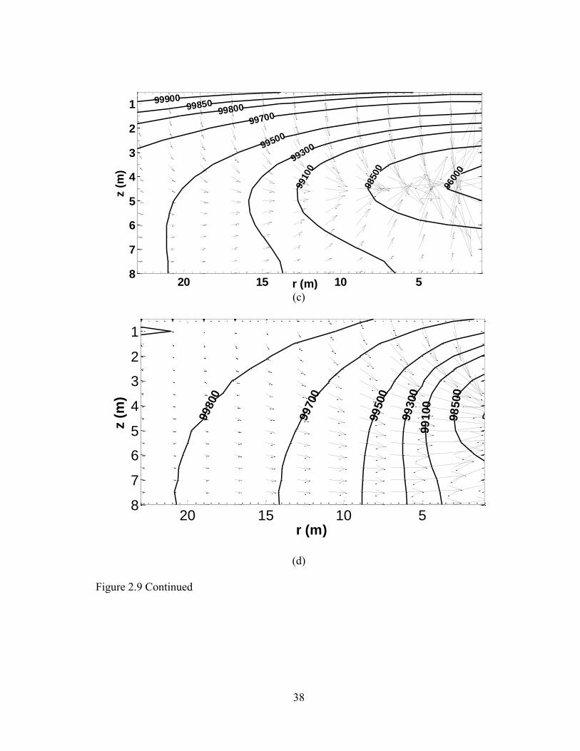
The gas pressure contour lines and gas flow lines at 0.7 days are drawn in Fig. 2.9. In

Figs. 2.9a, 2.9b and 2.9c, the gas pressures and pore gas flow velocities are calculated by

solution-1, where both the atmospheric pressure and water table effects are neglected,

and kr/kz are increased from 2.5 to 10, and to 25 with a fixing kr. In Figs. 2.9d, 2.9e and

2.9f, they are calculated by solution-3, where the atmospheric pressure effect is taken

into account, and kr/kz are increased from 2.5 to 10, and to 25 with a fixing kr. According

to Fig. 2.9, a higher value of kr/kz leads to a greater component of the pore-gas velocity

vector toward the gas pumping well located at r=0 and z=4.0~4.6 m, especially in the

unsaturated zone below the well screen (Figs. 2.9a-c and Figs. 2.9d-e). Besides, if the

gas pressure vacuum is defined by a certain value of the pressure contour line, for

37

5101520

1

2

3

4

5

6

7

8r (m)

z (

m)

99980

9995

0

99900

99850

99800

99

700

99

500

99

300

99

100

98

500

(a)

5101520

1

2

3

4

5

6

7

8r (m)

z (

m)

99950

99900

99850

99800

99700

9950

0

9930

0

9910

0

98500

9600

0

(b)

Figure 2.9 The gas pressure contour lines and gas flow lines at 0.7 day calculated by solution-1 (a) with kr/kz=2.5; (b) with kr/kz=10; (c) with kr/kz=25; and calculated by solution-3 (d) with kr/kz=2.5; (e) with kr/kz=10; (f) with kr/kz=25 by fixing kz.

38

5101520

1

2

3

4

5

6

7

8r (m)

z (

m)

9990099850

99800

99700

99500

99300

9910

0

9850

0

9600

0

(c)

5101520

1

2

3

4

5

6

7

8

r (m)

z (

m)

99800

99700

99500

99

300

99

100

98

500

(d)

Figure 2.9 Continued

39

5101520

1

2

3

4

5

6

7

8r (m)

z (

m)

99800

99700

9950099300

9910

0

9850

0

9600

0

(e)

5101520

1

2

3

4

5

6

7

8r (m)

z (

m)

99700

99500

9930

0

9910

0

98500

9600

0

(f)

Figure 2.9 Continued

40

example, 99500Pa, the gas pressure vacuum increases with the value of kr/kz (Figs. 2.9a-

c and Figs. 2.9d-e). Therefore, a higher value of kr/kz is favorable for SVE at non-coastal

sites. When comparing Figs. 2.9d-e with Figs. 2.9a-c, we find that the atmospheric

pressure extends the subsurface gas pressure contour lines outward away from the gas

pumping well, because the atmospheric pressure is below its average value at 0.7 day.

However, the atmospheric pressure does not change the gas flow lines much with

different values of kr/kz.

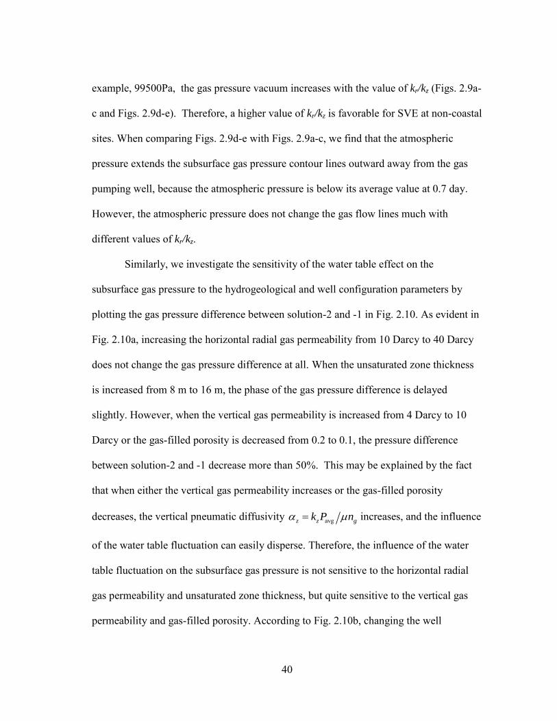
Similarly, we investigate the sensitivity of the water table effect on the

subsurface gas pressure to the hydrogeological and well configuration parameters by

plotting the gas pressure difference between solution-2 and -1 in Fig. 2.10. As evident in

Fig. 2.10a, increasing the horizontal radial gas permeability from 10 Darcy to 40 Darcy

does not change the gas pressure difference at all. When the unsaturated zone thickness

is increased from 8 m to 16 m, the phase of the gas pressure difference is delayed

slightly. However, when the vertical gas permeability is increased from 4 Darcy to 10

Darcy or the gas-filled porosity is decreased from 0.2 to 0.1, the pressure difference

between solution-2 and -1 decrease more than 50%. This may be explained by the fact

that when either the vertical gas permeability increases or the gas-filled porosity

decreases, the vertical pneumatic diffusivity avgz z gk P n increases, and the influence

of the water table fluctuation can easily disperse. Therefore, the influence of the water

table fluctuation on the subsurface gas pressure is not sensitive to the horizontal radial

gas permeability and unsaturated zone thickness, but quite sensitive to the vertical gas

permeability and gas-filled porosity. According to Fig. 2.10b, changing the well

41

0 1 2 3 4 5 6 7 8 9

x 104

-300

-200

-100

0

100

200

300

400

time (sec)

dra

wd

ow

n d

iffe

ren

ce (

Pa)

kr=10 Darcy, k

z=4 Darcy, n

g=0.2, h=8 m

kr=40 Darcy, k

z=4 Darcy, n

g=0.2, h=8 m

kr=10 Darcy, k

z=10 Darcy, n

g=0.2, h=8 m

kr=10 Darcy, k

z=4 Darcy, n

g=0.1, h=8 m

kr=10 Darcy, k

z=4 Darcy, n

g=0.2, h=16 m

(a)

0 1 2 3 4 5 6 7 8 9

x 104

-300

-200

-100

0

100

200

300

400

time (sec)

dra

wd

ow

n d

iffe

ren

ce (

Pa)

(a+b)/2=4.3 m, a-b=0.6 m

(a+b)/2=6.3 m, a-b=0.6 m

(a+b)/2=4.3 m, a-b=1.2 m

(b)

Figure 2.10 Figure 2.10 Comparison of the gas pressure difference between solution-2 and -1 at the observation points r=2 m, and z=4.3 m (a) with different hydrogeological parameters; (b) with different well configuration parameters.

42

configuration parameters does not change the influence of the water table fluctuation.

Fig. 2.11 shows the gas pressure contour lines and gas flow lines at 0.7 day

calculated by solution-2 at coastal sites where the water table effect is taken into account.

In Figs. 2.11a, 2.11b, and 2.11c, the values of kr/kz are increased from 2.5 to10, and to 25

with a fixing kz. As evident in Fig. 2.11, a downward moving water table decreases the

gas pressure in the unsaturated zone and extends the gas pressure contour lines outward

away from the gas pumping well. As the value of kr/kz increases, the pore-gas velocity is

directed more and more downward toward water table, except at the place close to and

right below the well screen. Besides, the magnitude of the pore-gas flow velocity

increases with the kr/kz value at greater distance from the well (for example r>12m),

while it decreases with the kr/kz value at the place close to the well (for example r>10m).

Therefore, a greater anisotropy (or a higher value of kr/kz) of the unsaturated zone is not

favorable for SVE with a downward moving water table at coastal sites. When

comparing Figs. 2.11a-c with Figs. 2.9a-c, we find that the higher the value of kr/kz, the

greater the influence of the water table in SVE.

One should note that in above sensitivity analysis, we do not explore the

sensitivity of the atmospheric pressure and water table effects on the subsurface gas

pressure to the parameters characterizing the atmospheric pressure and water table cycles.

That is because firstly the parameters describing the atmospheric pressure and water

table fluctuations in this study are chosen based on real conditions, and they are typical

values for the real world cases. Secondly, the sensitivity results to these parameters are

43

5101520

1

2

3

4

5

6

7

8r (m)

z (

m)

99950

99900

9985099800

99700

9950

0

9930

099100

98500

(a)

5101520

1

2

3

4

5

6

7

8

r (m)

z (

m)

9985099800

99700

99500

99300

99100

98500

9600

0

(b)

Figure 2.11 The gas pressure contour lines and gas flow lines calculated by solution-2 at 0.7 day (a) with kr/kz=2.5; (b) with kr/kz=10; (c) with kr/kz=25 by fixing kz at coastal sites.

44

5101520

1

2

3

4

5

6

7

8r (m)

z (

m)

9970099500

9930099100

98500

9600

0

(c)

Figure 2.11 Continued

quite obvious. For instance, increasing the magnitudes of the atmospheric pressure and

water table fluctuations increases their influence.

2.4 Summary and conclusions

This study presented a new semi-analytical solution to the subsurface gas

pressure distribution taking into account both the atmospheric pressure and water table

fluctuations for SVE in a homogenous but anisotropic unsaturated zone. To develop this

solution, the upper boundary of the system was set at the ground surface, where the gas

pressure equals the time-dependent atmospheric pressure instead of a constant average

pressure. The lower boundary was set at the water table, where the water table velocity

was introduced into the variable flux type boundary condition by applying Darcy’s law

45

to the water table instead of a gas-impermeable boundary. The developed new solution

was checked against a numerical solution developed in Comsol Multiphysics and was

found to be sufficiently accurate for the purpose of this study.

Solutions with different upper and lower boundary conditions were compared to

investigate the influence of the atmospheric pressure and water table fluctuations on the

subsurface gas pressure distribution and the ROI for SVE at both non-coastal and coastal

sites. The diurnal atmospheric pressure fluctuations at both non-coastal and coastal sites

were ideally described by a sinusoidal function with a magnitude of 150 Pa. The diurnal

water table fluctuation at a non-coastal site was ideally described by a sinusoidal

function with a magnitude of 0.02 m. The tidal-induced diurnal and semidiurnal water

table fluctuations at a coastal site were described by the summation of two sinusoidal

functions as found in Li and Jiao [2005] and Li et al. [2011]. Solutions were also

compared to investigate the sensitivity of the influence of the atmospheric pressure and

water table fluctuations on the subsurface gas pressure to the hydrogeological and well

configuration parameters.

According to this study, the following conclusions can be drawn:

1. In a non-coastal site where the daily water table fluctuation is in centimeters

scale, the water table effect is negligible but the atmospheric pressure effect should be

taken into account for the interpretation of gas pressure data. In a coastal site where the

daily water table fluctuation is in tens of centimeters scale, both the water table and

atmospheric pressure fluctuations need to be considered, and the errors induced from

neglecting their effects are amplified when the atmospheric pressure is increasing and

46

the water table is moving upward simultaneously, or when the atmospheric pressure is

decreasing and the water table is moving downward simultaneously.

2. The atmospheric pressure fluctuation mainly change the ROI defined by the

0.01 cm/s pore-gas velocity contour at the shallow depth. When the atmospheric

pressure is greater than its averaged value, the ROI at the shallow depth increases, and

vice versa. Generally, when the dimensionless atmospheric pressure square fD is greater

than 0.001, the atmospheric pressure effect should be considered to accurately interpret

active SVE.

3. The water table fluctuation changes the ROI for the gas pumping well across

the whole unsaturated zone. Either a downward or an upward moving water table with a

dimensionless velocity VwtD greater than 0.14 can greatly increase the ROI at the deep

unsaturated zone.

4. The influence of the atmospheric pressure fluctuation in SVE is sensitive to

the vertical gas permeability when its value is small (usually below 4 Darcy). If the

subsurface gas pressure drawdown is the difference between the subsurface gas pressure

and the current atmospheric pressure (i.e., a differential pressure transducer is used), the

atmospheric pressure fluctuation only has detectable influence on the subsurface gas

pressure distribution when the vertical gas permeability is small enough (0.4 Darcy for

the parameters in this study). The influence of the atmospheric pressure fluctuation is

insensitive to the horizontal radial gas permeability, gas-filled porosity, well depth, and

well screen length under the conditions of these simulations. The influence of the water

table fluctuation increases greatly with the decrease of the vertical gas permeability, gas-

47

filled porosity, and the vertical anisotropy of the unsaturated zone in the range of field

values. A greater vertical anisotropy is favorable for SVE at non-coastal sites but

unfavorable for SVE at coastal sites.

48

3. BAROMETRIC PUMPING IN A HOMOGENEOUS UNSATURATED ZONE*

3.1 Introduction

3.1.1 Barometric Pumping(BP)

As discussed in section 1.1, BP can either work as a stand-alone measure or in

conjunction with active SVE [Murdoch, 2000]. It has been field tested as an effective

soil remediation technology at several sites, including the US Department of Energy

(DOE) Savannah River site in Aiken, South Carolina, and the Hanford site in Richland,

Washington [Rohay et al., 1993; Rossabi et al., 993; Jennings and Patil, 2002; Riha,

2005]. However, few careful studies of its fundamentals, such as the gas flow rate and

mass removal effectiveness, have been conducted [Murdoch, 2000], which has hampered

the wide use of BP in field applications. Present available references include the studies

conducted by Ellerd et al. [1999], Rossabi and Falta [2002], Neeper [2003] and Rossabi

[2006]. Rossabi and Falta [2002] and Rossabi [2006] developed impulse-response

solutions for gas flow rate to/from a BPW for a one-layer soil system. Neeper [2003]

presented a harmonic analysis of gas flow rate for an open borehole in infinite strata with

different horizontal permeability. However, they all derived their 2-D gas flow solutions

by superimposing the solutions of two 1-D gas flow problems: the 1-D vertical gas flow

solution and the 1-D axisymmetric radial gas flow solution. Although sufficient accurate

for most field applications and computationally efficient, this treatment is not as

* Reprinted with permission from "A new solution and data analysis for gas flow to a barometric pumping well" by You, K., H. Zhan, and J. Li (2010), Adv. Water Resour., 33(12), 1444-1455, Copyright [2010] by Elsevier.

49

physically representative as a 2-D or 3-D model. Ellerd et al. [1999] described a 2-D

numerical study of gas flow in a three-layer soil system at the Hanford site.

3.1.2 Mixed-type boundary condition

A physically and mathematically reasonable description of the problem of gas

flow to/from a BPW should be a mixed-type boundary value problem (MBVP),

considering the gas impermeable boundary at the well casing and a uniform gas pressure

at the well screen. Up to present, the limited numbers of analytical solutions to the

MBVPs [Cassiani and Kabala, 1998; Chang and Chen, 2002, 2003; Change and Yeh,

2009]include the dual integral/series equation [Sneddon, 1966], Weiner-Hopf technique

[Noble, 1958], and Green’s function [Huang and Chang, 1984]. Most MBVPs are solved

numerically [Yedder and Bilgen, 1994] or by approximate methods such as asymptotic

analysis [Bassani et al., 1987] or perturbation techniques [Wilkinson and Hammond,

1990; Chang and Yeh, 2009]. Chang and Yeh [2009] derived an analytical solution for

the aquifer response to a constant-head test performed at a partially penetrating well

using the dual series equations and perturbation method, which is rather complicated to

use. Chang and Chen [2002,2003] obtained the solution to a flowing partially

penetrating well by transforming the mixed-type boundary into a homogenous Neumann

type boundary and discretizing the well screen into small segments. This method has

been proven to be reasonably accurate if the discretization of the well screen is fine

enough [Chang and Chen, 2002,2003]. This technique will be employed in our study

because of its simplicity.

50

3.1.3 Purpose and organization of the study

The purpose of this study is to present a 2-D semi-analytical solution to

subsurface gas pressure distribution and gas flow rate to/from a BPW with and without a

check valve in a homogenous unsaturated zone (hereinafter referred to as SA solution).

The paper is organized as follows. The first part is to derive a new 2-D semi-analytical

solution to subsurface gas pressure distribution and gas flow rate to a BPW and to

develop a 2-D finite element numerical solution using Comsol Multiphysics to compare

with the SA solution. The second part is to analyze the change of ROI with the

parameters describing the unsaturated zone properties and the specific well design and to

analyze the difference among the SA solutions with and without the installation of check

valves. The third part is to use the developed solution to interpret a field BP experiment

at the A/M area of the Savannah River site in Aiken, South Carolina. The last part is the

summary and conclusions. One should note that the parameters and equations defined in

section 3 only apply to section 3.

3.2 Physical and mathematical models

3.2.1 Pumping without a check valve

Fig. 3.1 shows the schematic diagram of gas flow to/from a BPW. The origin of

the coordinate system is at the ground surface. The z axis is vertical, positive downward

and through the axis of the BPW. The r axis is horizontally radial. The ground surface is

open to the atmosphere and has a Dirichlet type boundary with a known atmospheric

pressure f *(t). The water table is impermeable to gas flow. The open wellbore has a

known atmospheric pressure f *(t) across the well screen and is gas-impermeable across

51

the well casing. The BPW is not extremely deep so that gravitational effect and vertical

gas pressure difference inside the BPW are negligible. The lateral boundary is infinitely

far from the BPW, thus will not affect gas flow to/ from the well. We arbitrarily choose a

fixed-pressure boundary at the lateral infinity.

Land surface

Water table

r

z

h1

h2H

Check valvef *(t)

l

*(r,z,t)P

VOCs plume

Figure 3.1 Diagram of barometric pumping and the BPW in a homogenous unsaturated zone.

If the unsaturated zone is assumed to be anisotropic but homogeneous, the

governing equation for the transient gas flow problem can be written as [Falta, 1995]:

2

2

2

2

z

P

r

P

rr

P

t

Pz

rr

, (3-1)

avg* ),,(),,( PtzrPtzrP , (3-2)

52

where t is time (T); r, z are radial (horizontal) and vertical coordinates (L), respectively;

Pavg is average gas pressure which is often set as the average atmospheric pressure (ML-

1T-2); P*(r, z, t), P(r, z, t) are subsurface gas pressure and subsurface gas pressure

deviation from the average gas pressure at coordinate z and time t (ML-1T-2),

respectively; r , z are radial and vertical gas diffusivities in the unsaturated zone (L2T-

1), respectively, and are defined as:

S

PKr

r

avg ,

S

PK z

z

avg , (3-3)

where Kr, Kz are radial and vertical gas permeability (L2), respectively; is porosity

(dimensionless); S is gas phase saturation (dimensionless); is dynamic gas viscosity

(ML-1T-1).

It is notable that Eq. (3-1) is a linearized gas flow equation simplified from the

nonlinear one [Massmann, 1989]. Massmann [1989] indicated that if the gas pressure

change is less than 50% of the initial gas pressure, the error induced from this

linearization is less than 5%. The magnitude of diurnal atmospheric pressure fluctuations

seldom exceeds 3 mbar [Miller and Thompson, 1970], and the intense atmospheric

pressure variations associated with regional weather change seldom exceeds 20 mbar to

30 mbar [Massmann and Farrier, 1992], all of which are less than 5% of 1 bar.

The initial subsurface pressure is assumed to be uniform and equal to the average

gas pressure Pavg.

0)0,,( zrP . (3-4)

According to the former discussion, the boundary conditions can be expressed as

53

Hzz

P

Hz

,0 , (3-5)

0, zfP , (3-6)

rP ,0 , (3-7)

Hzhhzrrr

Pwrr w

21,0,,0| , (3-8)

21,, hzhrrfP w , (3-9)

where H is the water table depth (L); h1, h2 are the depths of the upper and lower ends of

the well screen (L), respectively; rw is the radius of the BPW (L); f is the atmospheric

pressure deviation from the average gas pressure Pavg (ML-1T-2) and is defined as

avg* Pff , (3-10)

where f* is the atmospheric pressure (ML-1T-2).

Eqs. (3-8) and (3-9) describe the boundary conditions along the well casing and

screen and belong to the Neumann and Dirichlet types, respectively, which depicts a

mixed-type boundary value problem. To solve this problem, one first transforms the

mixed-type boundary condition along the wellbore into a uniform Neumann type

boundary by replacing Eq. (3-9) with

21,),,(| hzhrrtzqr

PKwwrr

r

w

, (3-11)

where qw is an unknown gas flow specific discharge along the well screen (LT-1), which

is time and depth dependent.

Eq. (3-1) will be solved with the initial condition (3-4) and boundary conditions

(3-5)-(3-8) and (3-11). The obtained P will be a function of qw. After this, one can

54

substitute the true boundary condition at the well screen Eq. (3-9) into the obtained P to

determine the expression of qw. Therefore, the subsurface gas pressure P* and the gas

flow rate to/from the BPW Q(t) (L3T-1) are obtained. This technique has been tested by

Chang and Chen [2002,2003] to be reasonable and useful in solving mixed-type

boundary value problems.

Apply Laplace transform to Eqs. (3-1), (3-5)-(3-8), and (3-11), one obtains

2

2

2

2

z

u

r

u

rr

usu z

rr

, (3-12)

0),( zsfu , (3-13)

Hzz

uHz

,0| , (3-14)

ru ,0 , (3-15)

Hzhhzrrr

uwrr w

21,0,,0| , (3-16)

21,,| hzhrrK

q

r

uw

r

wrr w

, (3-17)

where s is Laplace transform parameter; overbar denotes variables in Laplace domain; u

is the counterpart of P in Laplace domain and is defined as

dtetzrPtzrPLszru st

0

),,(),,(),,( , (3-18)

where L is Laplace operator.

Apply finite Fourier transform to z in Eqs. (3-12)-(3-17), one has

fdvs

ddr

dv

rdr

vdn

r

z

r

n

r

z

)(1 2

2

2

, (3-19)

55

rv ,0 , (3-20)

dzzdK

q

dr

dvn

h

hr

wrr w

)sin(| 2

1

, (3-21)

where v is the finite Fourier transform of u and is defined as

dzzdszruszruFsnrvH

ng 0

)sin(),,(),,(),,( , (3-22)

Hndn

21 , n=1, 2,… , (3-23)

where Fg is the finite Fourier transform operator and n is a positive integer.

After parameter variation

r

n

r

zn

r

z sdfdvy

2 , Eq. (3-19)

becomes a modified Bessel equation and can be easily solved. The solution of Eq. (3-19)

subjected to Eqs. (3-20) and (3-21) is

2

1

)sin()(

)(),,(1

0 h

hnw

wrC

Ddzzdq

rCKCK

rCKsnrv

, (3-24)

where K0, K1 are the zero-order and the first-order modified Bessel functions of the

second kind, respectively; D and C are parameters defined as

fdDs

dC n

r

z

r

n

r

z

,2 . (3-25)

Applying inverse finite Fourier transform to Eq. (3-24), one obtains

)sin()sin()(

)(2),,(1 1

0 2

1

zdC

Ddzzdq

rCKCK

rCK

Hszru n

n

h

hnw

wr

. (3-26)

56

Now one has the solution for this mixed-type boundary value problem in Laplace

domain dependent on an unknown gas flow specific discharge at the wellbore, qw. In the

following, one can derive the expression for qw.

The well screen has a length of l (L) (l=h2-h1) and is discretized into M pieces of

segments, each having a length of ∆zi, i=1, 2, …, M. The length of each segment is so

small that qw is approximately uniform across this segment. Therefore, one has

)sin()sin(2

1

zddzzdq nn

h

hw

)sin()sin(...)sin()sin(11

1

211

11

2

221 zddzzdqdzzdqdzzdq n

zh

h

zzh

zh

h

zhnwMnwnw

M

)sin()cos()cos(1)( 11

zdzdzdd

sq ninin

n

M

i

wi

, (3-27)

where qwi is qw in the ith segment (LT-1) and overbar denotes its counterpart in Laplace

domain; zi is the depth of the lower end of the ith segment (L) (z0=h1). Substituting Eq.

(3-27) into Eq. (3-26), one gets

1

11

1

0

1

)sin(2

)sin()cos()cos()(

)()(2),,(

n

n

n

ninin

wn

M

i

wi

r

zdC

D

H

zdzdzdrCKCd

rCKsq

HKszru

. (3-28)

The boundary condition (3-9) in Laplace domain is

21,),(),,( hzhrrsfszru ww . (3-29)

Substituting Eq. (3-28) into Eq. (3-29), one has

57

),,( szru jw

111

1

0

1

)sin(2)sin()cos()cos()(

)()(2n

jn

n

jninin

wn

wM

i

wi

r

zdC

D

Hzdzdzd

rCKCd

rCKsq

HK

)(sf , (3-30)

where jz = (zj+zj-1)/2, j=1, 2,…, M. Rearranging Eq. (3-28) and setting

1

11

0 )sin()cos()cos()(

)(n

jninin

wn

wij zdzdzd

rCKCd

rCKa , (3-31)

fHK

zdC

DKb r

n

jnr

j 2

)sin(1

, (3-32)

one has

Mjbqa jwi

M

i

ij ...,,2,1,1

. (3-33)

By solving this matrix, one can get wiq . The gas flow rate to/from the BPW in

Laplace domain can be obtained using the following equation

i

M

i

wiw zsqrsQ

)(2)(1

, (3-34)

and the subsurface gas pressure in Laplace domain could be obtained by substituting the

acquired wiq into Eq. (3-24). One noticeable point is that when the well screen is equally

divided into M segments, matrix [aij] is symmetrical and the number of element in

matrix [aij] required to be calculated is M(1+M)/2; when the well screen is divided into

M segments with different lengths, matrix [aij] is a M×M unsymmetrical matrix and the

number of element in matrix [aij] required to be calculated is M2. Because of the

58

complexity of the expression forwiq , a simple closed-form expression for the subsurface

gas pressure and gas flow rate to/from the BPW in real-time domain cannot be obtained

easily. We adopted a numerical inverse Laplace transform program based on the de

Hoog algorithm [Hollenbeck, 1998] to calculate the subsurface gas pressure and gas flow

rate to/from the BPW in real-time domain. Matlab program 2-DGF is developed to assist

the computation including the matrix inversion and the inverse Laplace transform [Press

et al., 2007].

3.2.2 Pumping with a check valve

In field applications of barometric pumping, check valves are often installed to

increase the concentration of VOCs in the exhaled gas [Ellerd et al., 1999; Murdoch,

2000; Vangelas et al., 2010]. When the differential pressure drives the gas containing

VOCs out of the unsaturated zone to the atmosphere, the check valve is open; when the

differential pressure tries to drive fresh air from the atmosphere into the unsaturated zone,

the check valve closes. With the check valve installed, VOCs can flow out of the BPW,

while fresh air cannot flow into the contaminated soil zone and hence will not dilute the

VOCs concentration in the gas phase [Ellerd et al., 1999]. Therefore, the concentration

of VOCs in the extracted gas increases when a check valve is used.

When a check valve is installed in a BPW, the governing equations and boundary

conditions for gas flow during the period of an open valve are the same as those in

section 3.2.1. However, a different boundary condition at the well screen should be

employed during the period of a closed valve. Ellerd et al. [1999] used the no-flux

boundary across the well screen when the check valve is closed, while in this study, we

59

will use a different boundary condition across the well screen when the check valve is

closed. In the following, the mass conservation law will be used to derive the boundary

condition during the closed check valve period. When the check valve is closed, the

subsurface gas pressure and the gas flow rate across the well screen are assumed to be

independent of depth. This point will be elaborated later in section 3.2.3.

Setting Pc to be the control pressure (ML-1T-2). When f*(t)Pc , the check valve

is open; when f*(t)＞Pc , the check valve is closed. According to the mass conservation

law, one has

ww VVttQ 0)( , (3-35)

where 0 is the gas density in the BPW at the moment when the check valve is closed

(ML-3); is the gas density in the BPW after a short interval of time t when the check

valve is closed (ML-3); Vw is the volume of the gas in the BPW (L3). According to the

ideal gas law, one has

RT

MP

RT

MP mww ,000 , (3-36)

where P0w, M0 are the gas pressure (ML-1T-2) and mixed gas molecular weight (M(Mol)-1)

in the BPW at the moment when the check valve is closed, respectively; Pw, Mm are the

gas pressure (ML-1T-2) and mixed gas molecular weight (M(Mol)-1) in the BPW after the

check valve is closed, respectively; R is the ideal gas constant and equals 8.314

J/(Mol×K); T is the temperature in Kelvin (K). Because of the assumption of uniform

pressure distribution in the well, P0w and Pw equal the subsurface gas pressure across the

well screen and will be replaced by P0 and P* in the following discussion, respectively.

60

Because the VOCs concentration in the exhaled gas is usually very mall, less than 100

ppmv [Riha, 2005], the mixed gas molecular weight can be approximated by the clean

air molecular weight Mair.

airair0 , MMMM m . (3-37)

According to Darcy’s Law, the gas flow rate across the well screen Q(t) can be

calculated by

wrrr

wr

PKlrtQ

|2)(

. (3-38)

Because one has assumed that when the check valve is closed, the subsurface gas

pressure and gas flow rate across the well screen are independent of depth, the entire

well screen can be treated as one single segment. The volume of the BPW, Vw (L3) can

be calculated by

HrV ww

2 . (3-39)

Substituting Eqs. (4-36), (4-37)-(4-39) into Eq. (4-35) and letting 0t , one has

dt

dP

dr

dPP

wrr | ， (3-40)

w

rw

V

lKr

2 . (3-41)

As mentioned above, the magnitude of the atmospheric pressure deviation from

the average gas pressure is less than 5% of the average gas pressure. It is even less for

subsurface gas pressure because as the atmospheric pressure wave propagates into the

unsaturated zone, the magnitude of the pressure is damped and the phase is delayed

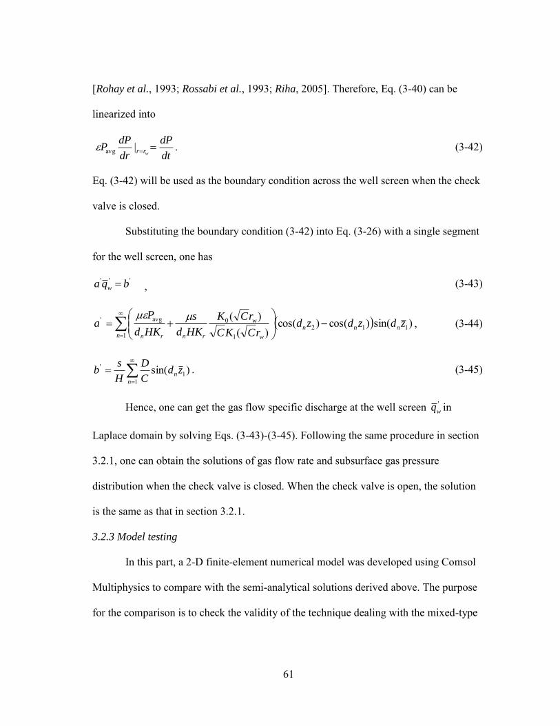
61

[Rohay et al., 1993; Rossabi et al., 1993; Riha, 2005]. Therefore, Eq. (3-40) can be

linearized into

dt

dP

dr

dPP

wrr |avg . (3-42)

Eq. (3-42) will be used as the boundary condition across the well screen when the check

valve is closed.

Substituting the boundary condition (3-42) into Eq. (3-26) with a single segment

for the well screen, one has

''' bqa w , (3-43)

1112

1

0avg' )sin()cos()cos()(

)(n

nnn

w

w

rnrn

zdzdzdrCKC

rCK

HKd

s

HKd

Pa

, (3-44)

1

1' )sin(

n

nzdC

D

H

sb . (3-45)

Hence, one can get the gas flow specific discharge at the well screen 'wq in

Laplace domain by solving Eqs. (3-43)-(3-45). Following the same procedure in section

3.2.1, one can obtain the solutions of gas flow rate and subsurface gas pressure

distribution when the check valve is closed. When the check valve is open, the solution

is the same as that in section 3.2.1.

3.2.3 Model testing

In this part, a 2-D finite-element numerical model was developed using Comsol

Multiphysics to compare with the semi-analytical solutions derived above. The purpose

for the comparison is to check the validity of the technique dealing with the mixed-type

62

boundary conditions used in sections 3.2.1 and 3.2.2. As an example, we report the

results for the barometric pumping without a check valve.

We compared the subsurface gas pressure distribution induced by barometric

pumping calculated by a 2-D axisymmetric numerical model developed in Comsol

Multiphysics with that calculated by two published 1-D analytical solutions in a

homogenous unsaturated zone. The two analytical solutions are 1-D vertical gas flow

and 1-D radial horizontal gas flow, respectively. At places where it is far away from the

BPW or deep enough in an unsaturated zone, the gas flow actually becomes 1-D vertical

flow or 1-D radial horizontal flow. Results show that if the grid is fine enough, the

numerical error for the model developed in Comsol Multiphysics is negligible. Thus in

the following discussion, solutions developed in Comsol Multiphysics will be treated as

the “accurate” solution, meaning that the numerical error is negligible for the purpose of

this study. The default setting for the model is listed in Table 3.1, which is modified

from Rossabi and Falta [2002]. We set the lateral boundary 500 m away from the well

and the gas pressure there is the average gas pressure Pavg. The ROIs for active SVE

with a mechanical pump are usually not larger than dozens of meters [Lee et al., 2002;

Dixon and Nichols, 2006]. The ROIs for BP should be even smaller, thus the chosen

lateral boundary is sufficiently far. Without losing generality, the input atmospheric

pressure is set to be idealized diurnal pressure cycles described by

)sin(avg* wtAPf , (3-46)

where A and w are the amplitude (ML-1T-2) and frequency (T-1) of diurnal atmospheric

pressure cycles, respectively. In this model, we set 250A Pa, and 86400/2w s-1.

63

The chosen amplitude is a typical diurnal barometric cycle [Miller and Thompson, 1970].

The maximum grid space along the well screen is set to be 0.1 m with a grid space

growth rate of 1.2.

Table 3.1 List of input parameters for gas flow in section 4.2.3, modified from Rossabi

and Falta [2002]. Parameters Values Gas-filled porosity ( S ) 0.2 Vertical permeability (Kz), m2 1×10-13 Radial permeability (Kr), m2 1×10-11 Viscosity ( ), kg m-1sec-1 1.8×10-5 Average gas pressure (Pavg), Pa 100,000 Well radius (rw), m 0.1 Unsaturated zone thickness (H), m 40.0 Depth of the upper end of the well screen (h1), m 33.0 Depth of the lower end of the well screen (h2), m 34.0

Fig. 3.2 shows the comparison of the total gas flow rate to/from the BPW without

a check valve in two days calculated by the numerical solutions and two kinds of SA

solutions, one treating the well screen as a single segment and the other dividing the well

screen into three segments (0.1 m, 0.8 m, 0.1 m). The two SA solutions match the

numerical solution very well, except at peak values, where the SA solutions deviate from

the numerical solution only slightly. Besides, the differences between the two SA

solutions are negligible. Our numerical exercises indicate that further increasing the

number of segments for the well screen to five does not improve the accuracy of

computation but increases the computational time. Therefore, the SA solution dividing

the well screen into three segments is sufficiently accurate for the case with an open

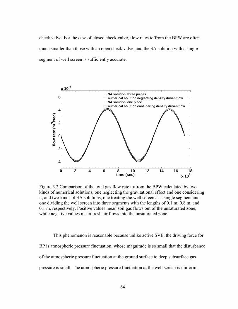
64

check valve. For the case of closed check valve, flow rates to/from the BPW are often

much smaller than those with an open check valve, and the SA solution with a single

segment of well screen is sufficiently accurate.

0 2 4 6 8 10 12 14 16 18

x 104

-4

-2

0

2

4

6

x 10-4

time (sec)

flo

w r

ate

(m

3/s

ec)

SA solution, three pieces

numerical solution neglecting density driven flow

SA solution, one piece

numerical solution considering density driven flow

Figure 3.2 Comparison of the total gas flow rate to/from the BPW calculated by two kinds of numerical solutions, one neglecting the gravitational effect and one considering it, and two kinds of SA solutions, one treating the well screen as a single segment and one dividing the well screen into three segments with the lengths of 0.1 m, 0.8 m, and 0.1 m, respectively. Positive values mean soil gas flows out of the unsaturated zone, while negative values mean fresh air flows into the unsaturated zone.

This phenomenon is reasonable because unlike active SVE, the driving force for

BP is atmospheric pressure fluctuation, whose magnitude is so small that the disturbance

of the atmospheric pressure fluctuation at the ground surface to deep subsurface gas

pressure is small. The atmospheric pressure fluctuation at the well screen is uniform.

65

Hence, the resulting gas flow velocity should be nearly uniform across the well screen,

except at the upper and lower ends of the well screen, where vertical gas flow is slightly

stronger. This is also the reason why we set the length of the two end segments much

shorter than the length of the middle segment when the well screen is discretized into

three or five segments. Such end effect of the well screen will have nearly negligible

influence upon the total flow rate, as one can see that the SA solution with a single

segment of well screen is nearly indistinguishable from the SA solution with three

segments of well screen (see Fig. 3.2). The deeper the well screen and/or the lower the

vertical gas permeability, the less the difference between the two SA solutions.

The numerical solution taking into account density driven (gravity) flow for

pumping without a check valve is also shown in Fig. 3.2. Obviously, its differences with

the SA solutions are also very small and can be neglected, which is reasonable because

of the small density of the air. This shows that the gravitational effect of gas flow can be

neglected.

Fig. 3.3 shows the comparison of the subsurface gas pressure at the depth of 33.5

m and at different distances from the well calculated by the 2-D numerical solution and

the SA solution treating the well screen as a single segment. The results from the SA

solution are almost the same as that from the 2-D numerical solution. Therefore, the

technique employed in dealing with the mixed-type boundary value problem in sections

3.2.1 and 3.2.2 can obtain reasonably good solution for barometric pumping.

66

0 2 4 6 8 10 12 14 16 18

x 104

0.9975

0.998

0.9985

0.999

0.9995

1

1.0005

1.001

1.0015

1.002

1.0025x 10

5

time (sec)

pre

ssu

re (

Pa)

f*(t)

r=0.3 m

r=0.6 m

r=1.1 m

Figure 3.3 Comparison of subsurface gas pressure at different distance from the well calculated by the numerical solution neglecting gravitational effect (solid lines) and the SA solution treating the well screen as a single segment (dashed lines) at the depth of 33.5 m.

3.3 Analysis

3.3.1 Radius of influence in pumping with a check valve

As discussed in section 2.3.2, ROI is one of the most important parameters in the

design of a SVE system. Because of the oscillatory characteristics of the driving force

(the atmospheric pressure fluctuation) for BP, there will not be a constant ROI during

operation. However, the analysis of pressure distribution near a BPW will give us some

idea about the ROI range in BP.

Before the BPW is drilled in the unsaturated zone, the atmospheric pressure wave

at the ground surface propagates into the unsaturated zone vertically and induces the

67

subsurface gas pressure fluctuation, whose amplitude is damped and phase is lagged

compared with the atmospheric pressure [Rohay et al., 1993; Rossabi et al., 1993; Riha,

2005]. When a BPW is installed, the subsurface gas pressure fluctuation will be induced

by the atmospheric pressure fluctuation not only at the ground surface but also at the

well screen.

Before the BPW is installed, the background gas pressure Pb(z, t) (ML-1T-2) in the

subsurface induced by the atmospheric pressure fluctuation at the ground surface can be

calculated by [Shan, 1995]

])1())[(cos()exp(2),(0

2avg wnz

n

unz

n

nb IaIzHataH

PtzP

, (3-47)

whereH

nan 2

)12( , **

0

* )cos()0,( dzzazPIH

nu , **2

0

* )exp()( dttatfI zn

t

w . The

pressure difference between the subsurface gas pressure P*(r, z, t) and the background

gas pressure Pb(z, t) at different time should give us some hint on the range of ROI.

For simplicity, the well screen is treated as one segment with a uniform gas flow

specific discharge. Fig. 3.4a shows the distribution of the absolute values of the pressure

difference, |(P*(r, z, t)-Pb(z, t))|, and Fig. 3.4b shows the distribution of the absolute

values of the dimensionless pressure difference, |(P*(r, z, t)-Pb(z, t))|/ (P*(rw, z, t)-Pb(z, t)),

with radial distance from the well at the depth of 33.5 m at different time. The same

values of parameters as used in section 3.2.3 are employed here, except that the

amplitude of the diurnal atmospheric pressure fluctuation is increased from 250 Pa to

500 Pa. Here we propose two new definitions for ROI. One defines the ROI as the

distance from the well where the gas pressure deviate a certain amount from the

68

subsurface background gas pressure (see Fig. 3.4a). The other defines the ROI as the

distance from the well where the magnitude of gas pressure fluctuation is a certain

percent of that at the well screen (see Fig. 3.4b). Figs. 3.4 show that ROI is not a

constant and depends on the atmospheric pressure fluctuation. If ROI is defined to be the

distance from the well where |(P*(r, z, t)-Pb(z, t))|/ (P*(rw, z, t)-Pb(z, t))=0.1, the range of

ROI is from 8 m to 11.5 m (Fig. 3.4b).

In order to obtain reliable ROI values, we recommend avoiding using data at the

time when the atmospheric pressure is close to its average gas pressure

( )0avg* Pff . For instance, t=1 day is the period of atmospheric fluctuation in Fig.

3.3, thus f (t=1 day) is zero, resulting in a value of |(P*(r, z, t)-Pb(z, t))| so small that the

calculation of ROI is less reliable for this time (Fig. 3.4a).

Besides time, ROI is also influenced by the unsaturated zone properties and the

design parameters for the BPW. Table 3.2 depicts the influence of the unsaturated zone

properties and BPW parameters on the range of ROI. When the effect of one parameter

is investigated, the other parameters are kept constant as in section 3.2.3. According to

Table 3.2, ROI increases with the radial gas permeability, and decreases with the vertical

gas permeability. The vertical gas permeability has larger effect on ROI. That is the

reason why a low permeable surface cover can increase the efficiency of BP [Ellerd et

al., 1999]. Adding such a cover not only substantially increases ROI but also increases

the flow rates to/from the BPW to a certain degree.

69

0 10 20 30 40 500

100

200

300

400

500

600

r (m)

|(P

*(r,

z, t)

-Pb(z

, t)

)| (

Pa)

t=0.2 day

t=1 day

t=0.4 day

t=0.6 dayt=0.8 day

(a)

Figure 3.4 (a) Distribution of the absolute values of subsurface gas pressure deviations from the subsurface background pressure |(P*(r, z, t)-Pb(z, t))| along the radial distance from the well at different time. (b) Distribution of the absolute relative values of subsurface gas pressure deviations from the subsurface background pressure |(P*(r, z, t)-Pb(z, t))|/ (P*(rw, z, t)-Pb(z, t)) along the radial distance from the well at different time.

70

0 10 20 30 40 500

0.2

0.4

0.6

0.8

1

r (m)

|(P

*(r,

z, t)

-Pb(z

, t)

)|/ (P

*(r w

, z, t)

-Pb(z

, t)

)

8 11.5

t=1 day

t=0.2 day

t=0.4 day

t=0.6 dayt=0.8 day

(b)

Figure 3.4 Continued

Table 3.2 Influence of unsaturated zone properties and BPW design parameters on the range of ROI.

Parameters Values Range of ROI (m) Radial permeability (Kr), Darcy

10 8.0-11.5 20 10.3-15.0 40 14.3-19.7

Vertical permeability (Kz), Darcy

0.025 15.0-33.4 0.05 11.2-22.8 0.1 8.0-11.5

Gas-filled porosity ( S )

0.2 8.0-11.5 0.4 15.0-30.0 0.8 15.0-32.5

Well depth ((h1+h2)/2), m

33.5 8.0-11.5 35.5 13.9-22.5 37.5 14.5-22.7

Length of the well screen (l), m

1.0 8.0-11.5 2.0 21.2-35.5 4.0 27-larger than 50

71

ROI increases with the gas-filled porosity when the gas-filled porosity is small.

However, when the gas-filled porosity is large enough (about 0.4 for the parameters of

Table 3.1), ROI is nearly independent of the gas-filled porosity. One noticeable point is

that 0.4 is usually much higher for the field gas-filled porosity of the fine grain

sediments. Thus, ROI increases with the gas-filled porosity in the range of values for the

field condition. The same pattern of change of ROI is found for the well depth which is

defined as the depth of the middle point of the well screen. ROI increases with the well

depth first and then remains unchanged with further increase of the well depth. That may

be caused by the fact that when the well depth is large enough, gas pressure at that depth

will not be influenced by the atmospheric pressure fluctuation at the ground surface, thus

gas flow to the BPW actually becomes a 1-D radial flow problem. ROI increases with

the length of the well screen. This may be caused by the fact that the definition of the

ROI in this study is based on the subsurface gas pressure at the depth of the middle point

of the well screen. When the well screen length increases, the gas flow at the depth of

the middle point of the well screen will be less influenced by the end effect. Thus, the

vertical flow will be reduced and the radial horizontal flow will increase. One should

note that this is only true for the gas flow in a homogenous media. If the media is much

heterogeneous, such as flow being confined in a thin layer between two lower

permeability layers, ROI will not change much with the increase of the well screen

length. The values of ROI also depend on its definition, as expected. For example, if

ROI is defined as the distance from the well when |(P*(r, z, t)-Pb(z, t))|/ (P*(rw, z, t)-Pb(z,

t))=0.2, the corresponding ROI will decrease. One noticeable point is that if the

72

transportation of VOCs is taken into account, the ranges of ROI will decrease for the

case of pumping without a check valve because of the plug flow at the time when gas

flow direction changes from out of BPW to into BPW. Besides, the discussion of ROI

based on pore gas flow velocity will be more appropriate according to the definition of

US EPA [1994].

3.3.2 Pumping with a check valve with different control pressure

When a check valve is installed in a BPW, the boundary condition at the well

screen alternates between a Dirichlet and a Cauchy type boundary. Accordingly, the gas

flow rate to/from the BPW changes not only with the atmospheric pressure fluctuation

but also with the specified control pressure (Pc), which acts as a threshold to open or

close the check valve. Usually, two kinds of control pressure can be used in BP. One is

the average gas pressure Pavg and the other is the subsurface background gas pressure

Pb(z, t) [Ellerd et al., 1999]. This part investigates influence of these two choices of

control pressure on gas flow rate. The same values of parameters used in section 3.2.3

are employed here except that the length of well screen is increased from 1 m to 3 m and

the amplitude of the diurnal atmospheric pressure fluctuation is increased from 250 Pa to

500 Pa in order to amplify the magnitude of the results and make the results more

obvious. For simplicity, the well screen is treated as a single segment.

According to Fig. 3.5a, when there is no check valve, soil gas flows out of the

unsaturated zone if the subsurface gas pressure is higher than the atmospheric pressure

and flows into the unsaturated zone if the subsurface gas pressure is lower than the

atmospheric pressure. When a check valve is installed, the gas flow rate has either zero

73

or positive values. When the check valve is closed, there is no gas flow across the well

screen except a very small flow rate at a short period of time immediately after the close

of the check valve. When the check valve is open, gas flows out of the unsaturated zone.

The values of the flow rate during this outflow period are the same as that for pumping

without a check valve.

0 2 4 6 8 10 12 14 16 18

x 104

-1.5

-1

-0.5

0

0.5

1

x 10-3

time (sec)

flo

w r

ate

(m

3/s

ec

)

pumping without check valve

pumping with check valve, Pc=P

avg

pumping with check valve, Pc=P

b(z,t)

(a)

Figure 3.5 Comparison of gas flow rate calculated by two SA solutions with a check valve when the well is at the depth of (a) 34.5 m and (b) 24.5 m, one using the average gas pressure as the control pressure and the other using the subsurface background gas pressure as the control pressure. Positive values mean soil gas flows out of the unsaturated zone, while negative values mean fresh air flows into the unsaturated zone.

74

0 2 4 6 8 10 12 14 16 18

x 104

-1.5

-1

-0.5

0

0.5

1

x 10-3

time (sec)

flo

w r

ate

(m

3/s

ec)

pumping without check valve

pumping with check valve, Pc=P

avg

pumping with check valve, Pc=P

b(z,t)

(b)

Figure 3.5 Continued

Fig. 3.5a exhibits that the results do not have noticeable difference whether the

check valve is controlled by Pavg or Pb(z, t). In order to see if this finding is affected by

the well depth, we decrease the well depth from 34.5 m to 24.5 m (Fig. 3.5b). One can

see that almost the same results as in Fig. 3.5a are obtained. Therefore, one can conclude

that the gas flow rate is not sensitive to the well depth, and it is also not sensitive to the

choice of the control pressure.

3.4 Field application

In this section, the developed SA solution without a check valve will be used to

interpret the field BP test at the A/M area of the Savannah River site in Aiken, South

Carolina. Savannah River site is located in Aiken, South Carolina and encompasses an

75

area of 800 km2 [Rossabi et al., 1993]. Trichloroethylene (TCE) and tetrachloroethylene

(PCE) were used as metal degreasing solvents for a nuclear material production facility

owned by the US DOE from 1951 until 1985 at this site. From 1958 to 1985, over two

million pounds of solvent containing TCE and PCE leaked into the 40 m thick

unsaturated zone because of leaks in a process sewer line [Rossabi et al., 1993]. This

unsaturated zone is composed of intervals of sand and clayed sand [Rohay et al., 1993].

Many remediation techniques were tested at this site, including active SVE, air sparge,

enhanced bioremediation, chemical oxidation and heating techniques. In order to test the

feasibility of BP technique at this site, many clusters of monitoring wells were used to

measure the naturally produced differential pressure between the subsurface gas and

surface air [Rohay et al., 1993; Rossabi et al., 1993; Rossabi and Falta, 2002]. Surface

and subsurface gas pressures in several unsaturated zone wells at different depths and

locations were monitored with a frequency of 0.1 Hz (averaged and stored every 10

minutes) at this site from 1993 to 1994. The gas flow rates to/from BPWs were also

measured with mass flow meters or a hot wire anemometer [Rohay et al., 1993].

In this study, the subsurface gas pressure and flow rate data measured in well

CPT RAM 16 will be used to interpret the field experiment because the available data set

for this well is most complete. The well depth is 32.2 m with a screened interval of 30

cm and an inner well radius of 1.27 cm. The average atmospheric pressure at the A/M

area of the Savannah River site is 100.4 kPa [Rossabi and Falta, 2002]. Because the SA

solution requires a continuous function to describe the input atmospheric pressure

fluctuation, but the field measured data are discrete, Fourier series analysis is employed

76

to transform the discrete data set into a smooth and continuous function. Our numerical

exercise shows that the first 150 terms in the Fourier series is sufficient for good fitting

of the measured atmospheric pressure data (see Fig. 3.6). In the field application, other

functions such as a piece wise smooth function obtained by connecting the atmospheric

pressure data point by point or a step function as in Rossabi and Falta [2002] can also be

employed to describe the atmospheric pressure fluctuation.

0 0.5 1 1.5 2

x 106

0.98

0.985

0.99

0.995

1

1.005

1.01

1.015

1.02x 10

5

time (sec)

pre

ssu

re (

Pa)

field measured atmospheric pressure

atmospheric pressure function obtained from Fourier series analysis

field measure subsurface gas pressure

subsurface gas pressure calculated by SA solution

Figure 3.6 Comparison of field measured atmospheric pressure and atmospheric pressure function obtained from Fourier series analysis, and comparison of field measured subsurface gas pressure and that calculated by the SA solution at the depth of 33.7 m.

Besides the atmospheric pressure data, parameters for the unsaturated zone

properties are also required to predict the well performance. We used the field measured

77

flow rate data during the first 2 days of a 23-day experiment to conduct parameter

optimization to search for the optimal values for the radial gas permeability Kr, vertical

gas permeability Kz and gas-filled porosity S . The simplex method is employed to do

the parameter optimization because of its simplicity and rapid convergence, and the gas

flow rate data rather than the subsurface gas pressure data are employed in parameter

optimization because of the computation efficiency. The 0.3 m long well screen is

discretized into three pieces of segments (0.05m, 0.2m, and 0.05 m) in the calculation.

One should notice that the results of parameter optimization may be non-unique.

However, a good initial guess of the results would lead to a rapid convergence to a

unique pair of results. The initial guess of Kr, Kz and S are 23 Darcy, 0.24 Darcy, and

0.16, respectively, which are based on the results of Rossabi and Falta [2002]. The

obtained optimal values for Kr and Kz are 19.8 and 0.21 Darcys, respectively, and S is

0.19.

It is worthwhile to point out that Rossabi and Falta [2002] gave the optimal

values of Kr and Kz to be 40 and 0.24 Darcys, respectively, using the same field data.

The values of Kz calculated from the SA solution and the solution of Rossabi and Falta

[2002] are almost the same. However, the Rossabi and Falta [2002] result for Kr is

almost twice of our result. This is because this study and the study of Rossabi and Falta

[2002] are based on different mathematical models. The SA solution in this study is

expected to be more accurate than the solution of Rossabi and Falta [2002] because it

honors the true nature of 2-D gas flow to a BPW. On the contrary, Rossabi and Falta

78

[2002] has used the superposition of a 1-D vertical flow and a 1-D horizontal radial flow

to approximate the actual 2-D flow problem.

The optimal values for Kr, Kz, and S are used to predict the gas flow rate and the

subsurface gas pressure at the depth of 33.7 m. According to Figs. 3.6 and 3.7, the

calculated subsurface gas pressure and gas flow rate match the field measured

counterparts well. But some details of dynamic changes are missing, which may be

caused by the homogeneity assumption for the unsaturated zone. As mentioned above,

the unsaturated zone at the study area is actually not homogenous and comprises of

interbedded sand and clayed sand. It is important to mention that the field data in this

section (Figs. 3.6 and 3.7) is actually a subset of that in Rossabi and Falta [2002] and

some more dynamic data may be missed.

The least square method was used to quantify the accuracy of the results

calculated by the SA solution. The RMSE for the subsurface gas pressure and flow rate

are 190 Pa and 2.99 L/min (=4.98 ×10-5 m3/sec), respectively, which are quite small

compared with the average fluctuation of the subsurface gas pressure and absolute value

of the average gas flow rate (Figs. 3.6 and 3.7). They are also smaller compared with

that of Rossabi and Flata [2002] solution, which are 213 Pa and 6.37 L/min (=1.06×10-4

m3/sec), respectively.

79

0 0.5 1 1.5 2

x 106

-5

0

5

x 10-4

time (sec)

flo

wra

te (

m3/s

)

field measured flowrate

calculate flowrate with 3 piece

calculated flowrate with 1 piece

Figure 3.7 Comparison of field measured gas flow rate to/from the BPW and that calculated by two kinds of SA solutions, one treating the well screen as a single segment with a length of 0.3 m and the other treating the well screen as three segments with the lengths of 0.05 m, 0.2 m, and 0.05 m, respectively. Positive values mean soil gas flows out of the unsaturated zone, while negative values mean fresh air flows into the unsaturated zone.

In order to explore how great the gas flow specific discharge changes across the

well screen, we also plot the gas flow rate calculated by using a single segment for the

0.3 m well screen. The results do not show any noticeable difference from the solution

obtained using three segments of well screen. Therefore, the gas flow specific discharge

can be approximated as uniformly distributed along the well screen for the purpose of

this study.

3.5 Summary and conclusions

A 2-D axisymmetric semi-analytical solution was developed to calculate the

80

subsurface gas pressure distribution and gas flow rate to/from a BPW with and without a

check valve installed in BP. The subsurface gas flow and gas pressure fluctuation were

induced by the atmospheric pressure fluctuation at the ground surface and at the screen

of the BPW. When a BPW is installed in the unsaturated zone, the boundary at the well

screen is the time-dependent atmospheric pressure, but at the well casing is impermeable

to gas flow. Thus, the gas flow in BP is a mixed-type boundary value problem. To solve

this problem, we first discretized the well screen into small segments, assuming each

segment had a uniform time-dependent unknown gas flow specific discharge across its

length, and transformed the mixed-type boundary condition at the well into a Neumann

type boundary condition. Based on this transformation, the solution in Laplace domain

was derived by finite Fourier transform technique. The obtained solution in Laplace

domain was employed to fit the fluctuating pressure at the well screen to derive the

expression for the unknown gas flow specific discharge and hence the subsurface gas

pressure and gas flow rate expression in Laplace domain. The numerical inverse Laplace

transform program was applied to obtain the time-domain subsurface gas pressure

distribution and gas flow rate. Pumping with a check valve installed was simulated by

modifying the boundary condition at the well screen to alternate between a Dirichlet and

a Cauchy type boundary condition derived from the mass conservation inside the BPW.

The technique in dealing with the mixed-type boundary condition was

demonstrated to be valid by a 2-D finite element numerical model developed in Comsol

Multiphysics, whose accuracy has been demonstrated by comparing with analytical

solutions under extreme conditions. This numerical model also showed that the gas flow

81

specific discharge changes only slightly across the well screen except at the two ends of

the well screen. It also shows that using a uniform distribution of gas flow specific

discharge across the well screen (single segment) will not introduce much difference

from that using variable distribution of gas flow specific discharge across the well screen

(multiple segments).

The developed SA solution for pumping without a check valve was used to

analyze the influence of the unsaturated zone properties and the BPW design scenario on

ROI. This solution is also applied to interpret the field BP experiment at the A/M area of

the Savannah River site in Aiken, South Carolina. The solution for pumping with a

check valve is employed to analyze the difference of the gas flow rate to/from a BPW

between the choices of two different control pressures: the average gas pressure and the

subsurface background gas pressure.

According to this study, the following conclusions can be drawn:

1. The mixed-type boundary value problem can be efficiently solved by the

technique of transforming it into a homogenous boundary type for 2-D gas flow to/from

a BPW.

2. The gas flow specific discharge varies slightly across the screen of the BPW.

The solution obtained by discretizing the well screen into three segments is sufficiently

accurate for gas flow to/from a BPW with an open check valve. The solution obtained by

treating the well screen as a single segment is sufficiently accurate for gas flow to/from a

BPW with a closed check valve.

82

3. The ROI in BP is time-dependent. It increases with radial gas permeability and

decreases with vertical gas permeability. It increases with gas-filled porosity in the

ranges of the values for the field condition. It increases with well depth if well depth is

small. However, it remains nearly unchanged if well depth is larger than a certain value.

ROI increases with the well screen length in a homogenous unsaturated zone.

4. The gas flow rates behave almost the same no matter the average gas pressure

or the subsurface background gas pressure is used as the control pressure for opening or

closing the check valve in a BPW.

5. The developed SA solution can accurately predict the subsurface gas pressure

distribution and gas flow rate in the field BP experiment at the A/M area of the

Savannah River site in Aiken, South Carolina. The root mean squares for both

subsurface gas pressure and gas flow rates are quite small compared with the

corresponding field data. The field data in this study is a subset of that in Rossabi and

Falta [2002] and some more dynamic data may be missed.

83

4. BAROMTERIC PUMPING IN A MULTI-LAYERED UNSATURATED ZONE*

4.1 Introduction

In section 3, We have investigated BP in a homogeneous unsaturated zone.

However, heterogeneity is ubiquitous in field unsaturated zones, and soil layers with

quite different properties are commonly present. The purpose of this study is to extend

the solution of soil gas flow rates to/from a BPW to a multilayered unsaturated zone

(hereinafter referred to as the ML solution) and to quantify the error induced from the

previous decomposing method. The developed new solutions will be tested by the

published field measurement data at the Hanford site in Richland, Washington, USA.

One should note that the parameters and equations defined in section 4 only apply to

section 4.

4.2 Mathematical models

The coordinate system is set up as follows. The origin is at water table. The z

axis is vertical, positive upward and through the axis of the BPW. The r axis is

horizontally radial. It is necessary to elucidate the physics of the flow system before the

mathematical modeling. The ground surface is the first-kind boundary condition with a

known air pressure Patm(t) which is time-dependent. The water table is impermeable to

gas flow. The open borehole has a known air pressure Patm(t) across the screened interval

and is gas-impermeable across the cast interval. The lateral boundary is assumed to be

*Reprinted with permission from "Gas flow to a barometric pumping well in a multilayered unsaturated zone" by You, K., H. Zhan and J. Li (2011a), Water Resour.

Res., 47, W05522, Copyright [2011] by Wiley.

84

infinitely far from the BPW, thus will not affect gas flow to/ from the well. We

arbitrarily choose a fixed-pressure boundary at the lateral infinity.

The same methodology used by Rossabi and Flata [2002], and Neeper [2003] for

dealing with soil gas flow to/from the BPW is employed in this study. First, the

subsurface gas pressure without the disturbance of the BPW is calculated from the one-

dimensional (1-D) vertical flow equation. Second, the so obtained subsurface gas

pressure is used as a background pressure to calculate the 1-D horizontal gas flow

to/from the BPW. One should be aware that this treatment is only an approximation in a

rigorous mathematical sense [Neeper, 2003].

4.2.1 Background pressure

In this section, we will derive the subsurface gas pressure response to the

barometric cycles at land surface in a three-layered unsaturated zone as an example.

Before a BPW is installed, the gas flow induced by the barometric cycles at land surface

should be 1-D vertical in all the three layers of the unsaturated zone, which can be

described as:

2

2

z

u

t

u ii

i

, (4-1)

avgii PPu , 3,2,1, iS

PK

ggii

avgzi

i

, (4-2)

where t is time (T); z is vertical coordinate (L); Pavg is average atmospheric pressure

(ML-1T-2); Pi is the subsurface gas pressures in the layer i (ML-1T-2); ui is the subsurface

gas pressure deviations from the average atmospheric pressure in the layer i (ML-1T-2);

85

g is the dynamic gas viscosity (ML-1T-1); i is the air diffusivities in the layer i (L2T-1);

Kzi, i and Sgi are the vertical permeability to air (L2), the soil porosity (dimensionless),

and the volumetric gas phase saturation (dimensionless) in the layer i, respectively.

It is notable that gravity effect is neglected in the governing equations above.

Because the average molecular weight of air and VOCs is low in barometric pumping,

neglecting the gravity effect is acceptable for the purpose of this study [Falta et al.,

1989], which has been validated in section 3.2.3.

The initial gas pressure in the three layers is assumed to be uniform and equal to

the average atmospheric pressure Pavg. Thus, one has

0)0,()0,()0,( 321 zuzuzu . (4-3)

The boundary conditions are

0,00

1

tz

u

z

, (4-4)

)()(),(3 tfPtPtBu avgatm , (4-5)

where B is the elevation of the land surface above the water table (L); f(t) is the arbitrary

function describing the atmospheric pressure deviation from the average atmospheric

pressure (ML-1T-2). Here we do not take into account the fluctuations of water table. This

effect is not important for aquifers in non-coastal sites, which has been discussed in

section 2.

The gas pressure and flux at the interfaces of layers are continuous and described

by

86

2,1,0|| 1 ituuii BziBzi , (4-6)

2,1,0|| 11

11

it

z

uK

z

uK

ii Bzi

ziBzi

zi, (4-7)

where B1 and B2 are the thicknesses of layers 1 and 2 (L), respectively; Kz1, Kz2 and Kz3

are the air permeability of layers 1, 2 and 3, respectively (L2).

Applying Laplace transform to the above equation group, one obtains

132

32

01 cosh)(

zz KK

A

fu , (4-8)

)(sinh)cosh()(sinh)sinh()(

12

132

321

21

31

31

02 BzA

KKBzA

KK

A

fu zzzz

,

(4-9)

)sinh()cosh()(sinh)cosh()sinh()(21

2

22

213

221

21

03 AA

KBBzAA

KK

A

fu zzz

)(cosh)sinh()sinh()(sinh 21

321

31

311

3

BBzAAKK

BBz zz

)(cosh)cosh()cosh( 21

321

321

32 BBzAAKK zz

. (4-10)

where

)sinh()cosh()sinh(,,, 32121

2103

332

221

11 AAA

KKABABABA zz

32

32321

31

31321

2

22 )cosh()sinh()sinh()sinh()sinh()cosh(

zzzzz KK

AAAKK

AAAK

)cosh()cosh()cosh( 321 AAA . (4-11)

87

The gas pressure in the real-time domain can be calculated using a numerical

inverse Laplace transform program such as the de Hoog algorithm [Hollenbeck, 1998].

We developed a MATLAB program Gas-W to facilitate the computation. The

subsurface gas pressure in a multilayered unsaturated without the disturbance of the

BPW can be calculated by adding or deleting governing equations like in Eqs. (4-1)-(4-2)

and continuity equations like in Eqs. (4-6)-(4-7).

4.2.2 Gas flow rate to/from the BPW

When a BPW exists, gas flow becomes 2-D.However, since the local vertical

pressure gradient is much smaller than the local radial pressure gradient near the well in

a deep unsaturated zone, the gas flow close to the well could be described as 1-D

horizontal flow [Rossabi and Falta, 2002; Neeper, 2003].The solution in the Laplace

domain for the 1-D horizontal gas flow is expressed as:

)/()/()(),(

0

*0*

K

rKsrs wb , (4-12)

where ),(),,(),( 0 tzPtzrPtrs ; 2wggavgr rSPK ; *r is the dimensionless radial

coordinate and wrrr * ; Kr is the horizontal permeability to air (L2); rw is the well

radius (L); is the Laplace transform parameter; over bar denotes variables in the

Laplace domain; K0 is the zero-order, second kind modified Bessel function. The

detailed development of the 1-D horizontal flow model could be found in Rossabi and

Falta [2002].

According to Duhamel’s theorem [Carslaw and Jaeger, 1959, p.30] and Hantush

[1964], the inverse Laplace transform for Eq. (4-12) is:

88

trtAtstrs wb /),()(),( ** , (4-13)

where is the sign of convolution and ),( A is called the flowing well function for

non-leaky aquifers and is defined by [Hantush, 1964]:

u

duu

uYuJ

uJuYuYuJA )exp(

)()()()()()(21),( 2

0 20

20

0000

, (4-14)

where J0 and Y0 are the first kind and second kind zero-order Bessel functions,

respectively.

Eq. (4-13) is the ML solution for pressure and it is different from the previous

Rossabi and Falta [2002] solution. Convolution is used to derive Eq. (4-13) from Eq. (4-

12), while Rossabi and Falta [2002] solution instead uses a direct multiplication of

)(tswb and ),( *rtA (see Eq. (11) in Rossabi and Falta [2002]). The ML solution

presented here is mathematically more rigorous than Rossabi and Falta [2002] solution.

Substituting Eq. (4-14) into Eq. (4-13) leads to:

0 20

20

*00

*002

0

*

)()()()()()(])(exp[)(2),(

udud

uYuJ

urJuYurYuJutstrs

t

wb . (4-15)

The total flow rate is

1*

*

* ),(2)(

rg

r

r

trsKbtQ

dudu

uYuJ

uYuJuJuYuts

Kb t

wb

g

r 22

02

0

10102

0 0 )()()()()()(])([exp)(4

, (4-16)

where b is the length of the well screen (L). One needs to note that the rigorous

calculation of gas flow rate should use the integration of the gas flow velocity across the

89

well screen. However, our numerical exercise shows when the well screen is deeper than

30 m, there is no obvious change of gas flow velocities across the well screen. Therefore,

the calculation of Eq. (4-16) is reasonable.

We compared the solution developed for a single-layered unsaturated zone using

decomposing method with the a 2-D numerical solution developed in Comsol

Multiphysics. Results show that the decomposing method always underestimates gas

flow rate to/from the BPW (Fig. 4.1). When the gas flow rate is within half of its peak

values, the error is almost undetected. It increases with the increase of gas flow rate (Fig.

4.1). The maximum error induced is about 20% and happens when the gas flow rate is at

its peak values (Fig. 4.1).

0 2 4 6 8 10 12 14 16 18

x 104

-4

-2

0

2

4

6

x 10-4

time (sec)

avera

ge v

elo

cit

y (

m/s

ec)

2D numerical solution

ML solution

Figure 4.1 Comparison of average gas flow velocity across the wellbore calculated by ML solution and 2-D numerical solution in a single-layered unsaturated zone.

90

4.3 Field application

In this part, the ML solution is used to simulate the subsurface gas flow rates

to/from the BPW in a three-layered unsaturated zone at Hanford site in Richland,

Washington. The Hanford site was a former US DOE plutonium production facility, and

carbon tetrachloride was used to recover plutonium from aqueous waste. From 1955 to

1973, about 368 to 580 m3 of liquid carbon tetrachloride was discharged into the

unsaturated zone at three primary disposal sites. As much as 65% of the released carbon

tetrachloride remained in the unsaturated zone [Ellerd et al., 1999].

The depth to water table at Hanford site is about 66 m. The stratigraphy in the

unsaturated zone consists of three distinctive layers. The upper layer is composed of

permeable sand and gravel with a thickness of 38 m, the intermediate layer is made up of

less permeable silty sand with a thickness of 8 m, and the lower layer consists of gravel

and sand interfingering with fine grained silt and clay with a thickness of 20 m. The

carbon tetrachloride in the unsaturated zone mainly concentrates in the intermediate low

permeable layer and the upper part of the lower layer. The upper, intermediate and lower

layers are referred to as layers 3, 2 and 1, respectively, and are characterized by

properties listed in Table 4.1. A BPW was located at 61.5 m depth in layer 1, screened

from depths of 58 m to 61.5 m, and had a diameter of 0.15 m. Details of the site

information can be found from Ellerd et al. [1999].

The input atmospheric pressure fluctuations are shown in Fig. 4.2, which were

collected at one-hour intervals during a 500-hour period. The discrete atmospheric

pressure data are treated by the same method as in Shan et al.[1999]. Fig. 4.2 also

91

presents the calculated subsurface gas pressure response by using the ML solution at the

depth of 59.75 m in layer 1. As can be seen, the magnitude of the subsurface pressure is

attenuated and the phase is delayed. The daily fluctuations of atmospheric pressure

cannot be detected and only the long period increasing/decreasing of atmospheric

pressure can propagate into the deep depth. This result is the same as that in previous

studies.

Table 4.1 List of input parameters for gas flow in a three-layered unsaturated zone. Parameters Layer 1 Layer 2 Layer 3 Gas-filled porosity (ng) 0.35 0.43 0.35 Thickness, m 20 8 38 Vertical permeability (Kz), m2 4.23×10-11 1.13×10-13 9.88×10-12 Radial permeability (Kr), m2 1.27×10-10 Viscosity ( g ), kg m-1sec-1 1.8×10-5 Average pressure (Pavg), Pa 99,407 Well radius (rw), m 0.15

Fig. 4.3 shows the comparison between the measured and calculated (using the

ML solution) gas flow rates. Generally, the calculated flow rates match the observed

data well. But at certain peak flow rates, for instance at time from 2×105 sec to 4×105 sec,

the calculated flow rates were larger than the observed ones. Besides, the root mean

square error (RMSE) for the flow rates is 0.0019 m3/sec, which is relatively large

compared with the average flow rates (see Fig. 4.3). This is partially because the

measured flow rates greater than 0.01 m3/sec were not recorded due to instrumentation

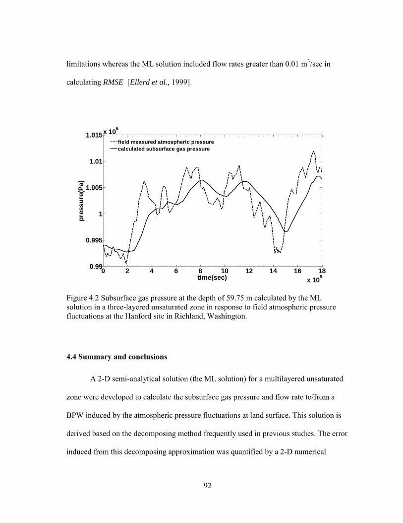
92

limitations whereas the ML solution included flow rates greater than 0.01 m3/sec in

calculating RMSE [Ellerd et al., 1999].

0 2 4 6 8 10 12 14 16 18

x 105

0.99

0.995

1

1.005

1.01

1.015x 10

5

time(sec)

pre

ssu

re(P

a)

field measured atmospheric pressure

calculated subsurface gas pressure

Figure 4.2 Subsurface gas pressure at the depth of 59.75 m calculated by the ML solution in a three-layered unsaturated zone in response to field atmospheric pressure fluctuations at the Hanford site in Richland, Washington.

4.4 Summary and conclusions

A 2-D semi-analytical solution (the ML solution) for a multilayered unsaturated

zone were developed to calculate the subsurface gas pressure and flow rate to/from a

BPW induced by the atmospheric pressure fluctuations at land surface. This solution is

derived based on the decomposing method frequently used in previous studies. The error

induced from this decomposing approximation was quantified by a 2-D numerical

93

solution developed in Comsol Multiphysics. Results show that the decomposing method

induces error as much as 20% for calculating gas flow rate at its peak values. However,

for low gas flow rates, this approximation method works reasonable well. The ML

solution extends the existing Rossabi and Falta [2002] solution to a multilayered

unsaturated zone. It also provides a more rigorous solution of the governing equations,

using convolution instead of direct multiplication. This solution was demonstrated to be

sufficient to predict the subsurface gas pressure changes and gas flow rates to/from a

BPW induced by the atmospheric pressure variations by the barometric pumping test at

the Hanford site in Richland, Washington, USA.

0 2 4 6 8 10 12 14 16 18

x 105

-0.015

-0.01

-0.005

0

0.005

0.01

0.015

time(sec)

flo

wra

te(m

3/s

ec)

field measured flow rates

calculated flow rates

Figure 4.3 Comparison of gas flow rate calculated by the ML solution with measured flow rates in a three-layered unsaturated zone in response to field atmospheric pressure variations at the Hanford site in Richland, Washington.

94

5. TRANSPORT MECHANISMS OF GAS PHASE VOLATILE ORGANIC

COMPOUNDS (VOCS) IN NATURAL ATTENUATION*

5.1 Introduction

Under natural conditions, the gas phase VOCs in the unsaturated zone can be

transported by the molecular diffusion and the advective flux. Molecular diffusion has

been believed to dominate the transport of the gas phase VOCs in the unsaturated zone

[Karimi et al., 1987; Marrin and Kerfoot, 1988; Smith et al., 1990; Conant et al., 1996].

The advective transport of VOCs is usually neglected in natural attenuation processes

[Wetherold et al., 1986; Batterman et al., 1992; Baehr and Baker, 1995]. However,

Thornstenson and Pollock [1989] found that the advective fluxes of VOCs could be

much greater or equal to the diffusive fluxes with a pressure gradient as small as 1 Pa m-

1 in an unsaturated zone with an air permeability of 10-12 m2 [Choi and Smith, 2005].

The advective transport of VOCs can be induced by the water table and

atmospheric pressure fluctuations. The water table fluctuation varies the gas pressure in

the unsaturated zone and drives the vertical movement of VOCs [Li and Jiao, 2005; Li et

al., 2011; You and Zhan, 2012]. In active SVE, the water table fluctuation has negligible

influence on the subsurface gas flow in non-coastal sites because of its small magnitude

(in the order of several centimeters) [You and Zhan, 2012]. However, in coastal sites, the

magnitude of the water table fluctuation is in several dozens of centimeters, and the gas

*Reprinted with permission from "Comparisons of diffusive and advective fluxes of gas phase volatile organic compounds (VOCs) in unsaturated zones under natural conditions" by You, K., and H. Zhan (2013), Adv. Water Resour., 52, 221-231, Copyright [2013] by Elsevier.

95

flow fields could be significantly altered [You and Zhan, 2012].

BP is defined as the vertical movement of gas in the subsurface induced by the

atmospheric pressure fluctuation. As discussed in section 3 and 4, when the atmospheric

pressure is higher than the gas pressure in the subsurface, the fresh air moves into the

subsurface, brings into oxygen and accelerates the biodegradation of VOCs. When the

atmospheric pressure is lower than the gas pressure in the subsurface, the contaminated

gas moves upward into the atmosphere and brings out the gas phase VOCs. Therefore,

the concentration of VOCs decreases gradually during this inhale and exhale process.

Studies by Nilson et al. [1991] indicated that rates of the barometric transport were one

or two orders of magnitude greater than the molecular diffusion in the fractured

permeable medium. Pirkle et al. [1992] presented that barometric pumping was the

primary cause of the vertical migration of contaminants into the atmosphere. Auer et al.

[1996] demonstrated that barometric pumping can significantly decrease the retention

time of volatiles in soil by enhancing the hydrodynamic dispersion. However, Nilson et

al. [1991] and Lowry et al. [1995] argued that no net transport of contaminant gases

occurred by barometrically-induced advective forces over time. Choi and Smith [2005]

also demonstrated that the diffusive flux was generally greater than the advective flux by

several orders of magnitude. Our hypothesis is that the importance of the barometrically-

induced advective transport relative to the diffusive flux may vary significantly with

field hydrogeological conditions [Massman, 2006].

The purpose of this study is to conduct a comprehensive investigation of the

relative significance of the gas phase VOCs transport mechanisms in the unsaturated

96

zone under various hydrogeological conditions. In most of the previous studies, the

pressure-driven advective flux or the density-driven advective flux of VOCs is neglected.

The density-driven flux dominates the gas phase transport of VOCs with high vapor

pressures and molecular weights in an unsaturated zone with high permeability [Falta et

al., 1989; Mendoza and Frind, 1990a, 1990b]. However, this conclusion is obtained

under a constant boundary pressure condition. This study differs from the previous ones

by the fact that all the three transport mechanisms, the diffusive flux, the pressure-driven

advective flux, and the density-driven advective flux, are brought into one gas flow and

mass transport model under variable pressure boundary conditions. To the best of our

knowledge, previous studies only take into account one or two of the three transport

mechanisms discussed here.

This study is organized as follows: in section 5.2, a one-dimensional (1D)

vertical gas flow and transport model taking into account the diffusive and the pressure-

driven and density-driven advective fluxes will be developed and solved by the finite-

difference method; in section 5.3, the developed model will be employed to investigate

the dominate transport mechanisms of the gas phase VOCs under various

hydrogeological conditions; in section 5.4, we will apply the developed solution to

interpret the trichloroethylene (TCE) contamination in the unsaturated zone at Picatinny

Arsenal in Morris County, New Jersey; this study is ended with a brief conclusion in

section 5.5. One should note that the parameters and equations defined in section 5 only

apply to section 5.

97

5.2 Physical and mathematical models

5.2.1 Gas flow in the subsurface

The origin of the coordinate system is set at the ground surface. The z axis is

vertical and positive downward. Before we progress further, it is better to illustrate the

physics first. The model for VOCs transport contains two parts: the gas flow equation to

calculate the advective transport velocity and the mass transport equation to calculate the

concentration of VOCs in the subsurface. The unsaturated zone has a thickness of h. The

upper boundary is set at the ground surface, where the atmospheric pressure fluctuates

regularly. The lower boundary is set at the water table, which also fluctuates with the

change of the pressure, temperature or infiltration. The VOCs are in the form of gas

phase, dissolved phase (water phase) and adsorbed phase (solid phase) in the unsaturated

zone. The non-aqueous liquid phase of VOCs is neglected because we assume the

contaminated ground water is the source of VOCs in the unsaturated zone.

Based on the ideal gas law and the Darcy’s law, the governing equation for 1D

vertical gas flow in the subsurface could be written as

)]([avg

gz

Pk

zt

P

P

Sg

gg

, (5-1)

where t is time (T); z is the spatial coordinate (L); P is the gas pressure in the subsurface

(M L-1T-2); Pavg is the average gas pressure (M L-1 T-2); g is the gravity acceleration

coefficient (LT-2); g is the gas phase density (ML-3), and

RTPM

MM

C airairgg )1( [Falta et al., 1989]; Cg is the concentration of the

VOC in the gas phase (ML-3); M and Mair are the molecular weights of the VOC and

98

clean air (M(mol)-1), respectively; R is the ideal gas constant, and R=8.314 J mol-1 K-1; T

is temperature (K); is porosity (dimensionless); Sg is the gas phase saturation

(dimensionless); is the gas dynamic viscosity (ML-1T-1); kg is the gas phase

permeability (L2).

Compared with the common gas flow equation in the unsaturated zone [Choi and

Smith, 2005], there is an additional term )( gk

zg

g

in Eq. (5-1), which accounts for

the density-driven flow in the subsurface.

At the ground surface, the gas pressure equals the atmospheric pressure which is

expressed as

0),(atm ztPP , (5-2)

where Patm is the time-dependent atmospheric pressure (ML-1T-2). There are generally

two types of atmospheric pressure fluctuation. One is the irregular transit of a cold/warm

front, which is ideally described by a first-order linear function [You and Zhan, 2012].

The other is the diurnal fluctuation induced by solar/terrestrial heating and cooling

effects, which is ideally described by a sinusoidal function as in Eq. (5-17) [You and

Zhan, 2012].

Applying the Darcy’s law to the water table, one could get the following lower

boundary condition

)(|)( wt tVgz

Pkhzg

g

, (5-3)

99

where Vwt is the time-dependent water table moving velocity (LT-1); h is the time-

dependent water table depth (L). Water table fluctuation could be induced by

temperature variations, atmospheric pressure fluctuations, seasonal variations of

precipitation, evapotranspiration, etc. [You and Zhan, 2012]. The velocity of the daily

water table fluctuation could be ideally described by Eq. (2-19).

Assuming the air in the unsaturated zone is initially in static equilibrium, one has

0,)( airavg tgzPzP , (5-4)

where air is the clean air density (ML-3). One should note that if the density-driven flow

is neglected, the initial gas pressure in the subsurface should equal Pavg for static

equilibrium condition.

5.2.2 Mass transport in the subsurface

As has been discussed in section 5.2.1, the VOCs in the unsaturated zone are in

the form of gas phase, water phase and solid phase. Assuming the VOC in each phase is

in chemical equilibrium [Chen et al., 1995; Choi and Smith, 2005], one has

g e wC H C , (5-5)

oc ocs b wC K f C , (5-6)

where Cw and Cs are the concentrations of the VOC (ML-3) in water phase and solid

phase, respectively; He is the Henry’s law constant (dimensionless); b is the soil bulk

density (ML-3); Koc is the organic carbon partition coefficient (L3M-1); foc is the weight

fraction of the organic carbon in soil (dimensionless). The equilibrium state is rarely

reached in field experiments [Abriola, 1989], especially between the solid and water

100

phases [Smith et al., 1990; Cho et al., 1993; Smith et al., 1996]. However, the

equilibrium assumption is widely used in previous published studies for the purpose of

simplicity. Because the aim of this study is to explore the relative importance of each

transport mechanism, we will still employ the equilibrium assumption in our study. The

influence of the dynamic mass transfer among different phases of VOCs will be studied

separately.

If the gas phase of the VOC is the only mobile phase, the governing equation for

the transient transport of the VOC in the unsaturated zone could be written as

[Armstrong et al., 1994]:

)()()( effococ

ggg

g

g

g

e

b

e

wg VC

zz

CD

zt

C

H

fK

H

, (5-7)

where Deff is the effective diffusion coefficient (L2), and 3.15.20eff /gDD [Choi et al.,

2002]; D0 is the free-air molecular diffusion coefficient of the VOC (L2); w wS ; Sw is

the water phase saturation (dimensionless); Vg is the pore-gas velocity (LT-1), and can be

calculated from the Darcy’s law as follows

)(z

Pg

kV g

g

g

g

. (5-8)

Gas phase dispersion is considered negligible compared with diffusion [Massmann and

Farrier, 1992; Choi and Smith, 2005].

The concentration of the VOC at the ground surface is set to be zero by assuming

a fast mixing process in the atmosphere [Choi and Smith, 2005]. Therefore,

.0,0 zCg (5-9)

101

The presence of a stagnant boundary layer at the ground surface can be easily integrated

into the model by replacing Eq. (5-9) with Eq. (58) in Sleep and Sykes [1989]. When the

ground surface is impermeable, the boundary condition of 0 zCg should be used

[Sleep and Sykes, 1989]. The gas phase concentration of VOC at the water table (Kg m-3)

is fixed to be constant Cwt

HzCCg ,wt . (5-10)

Initially, assuming the concentration of the VOC increases from zero at the ground

surface to the water table with a constant gradient of Cz (Kg m-4) [Choi and Smith,

2005]. Therefore, the initial condition is expressed as

0, tzCC zg . (5-11)

Solutions to the gas flow and mass transport equations are obtained numerically

by a MATLAB program called 1D-VT based on the explicit finite-difference method

using the Lax-Wendroff scheme, where artificial dispersion terms are added to the

discretized governing equations to compress the numerical dispersion. Detailed

information about this scheme can be found in Fletcher [1991]. One should note that the

problem discussed above could be simulated by many multiphase flow models. However,

we developed our own numerical solution because it is easier for us to control some

parameters, for example, the moving lower boundary condition.

5.2.3 Model verification

In this section, we will check the accuracy of the above developed solution 1D-

VT by comparing with analytical solutions under certain conditions. If the gravity effect

102

is neglected (g=0 in Eq. (6-1)), and the velocity of the water table fluctuation Vwt=0, the

analytical solution to the subsurface gas pressure variation induced by the atmospheric

pressure fluctuation expressed in Eq. (2-17) could be found in Shan [1995]. Our

numerical exercises show that the differences between the subsurface gas pressure

calculated by 1D-VT and the analytical solution are undetectable at all depths.

Lapidus and Amundson [1952] and van Genuchten and Parker [1984] provided

an analytical solution to the solute transport in an infinite column with a constant inlet

solute concentration and a no-flux outlet boundary condition. If we set an arbitrarily

constant pore-gas velocity for all the depth and a constant upper boundary concentration

to 1D-VT, fix the velocity of water table fluctuation Vwt=0, neglect the gravity effect and

set the average depth of the unsaturated zone H to be large enough, the numerical

solution calculated by 1D-VT should be the same with the analytical solution in Lapidus

and Amundson [1952] and van Genuchten and Parker [1984]. Our numerical exercises

show that the differences between the breakthrough curves calculated by the analytical

solution and 1D-VT are negligible. Therefore, 1D-VT is expected to be accurate enough

for the purpose of this study.

5.3 Field application

In this section, the developed model 1D-VT is applied to interpret a field study of

TCE transport in natural attenuation at Picatinny Arsenal in Morris County, New Jersey.

About 1.26×105 m2 of the unconfined aquifer at this site was contaminated by TCE

with a concentration of greater than 10 mg L-1 resulting from improper disposal practices

of metal degreasing and cleaning operations from 1960 to 1981 [Choi et al., 2002].

103

Extensive field studies have been conducted to investigate the TCE contamination in the

unsaturated zone at the site. The unsaturated zone mainly consists of medium-to-coarse

sand with low organic carbon contents ranging from 0.080% to 1.020% [Choi et al.,

2002]. The 1998 sampling event took place at a site where the unsaturated zone had an

average thickness of 3.2 m, a porosity of 0.32 and an average moisture content of

0.117[Choi et al., 2002]. During the sampling process, no precipitation occurred and the

magnitude of the water table fluctuation was less than 2 cm [Choi et al., 2002]. The

detailed information could be found in Smith et al. [1996] and Choi et al. [2002].

In our study, the molecular weight, dimensionless Henry's law constant, organic

carbon partition coefficient and diffusion coefficient of TCE are set to 131.4 g mol-1,

0.28, 0.735 m3 Kg-1 and 0.0787 cm2 s-1 [Chiao et al., 1994], respectively. TCE

concentration at the water table is set to be 2 mg L-1, and initially it decreases linearly to

0 at the ground surface with a constant concentration gradient of 0.625 mg L-1 m-1 , as

used by Choi et al. [2002]. Besides the data above, the gas phase permeability and the

parameters for the water table fluctuation are also required to predict the transport of

TCE in the unsaturated zone. We used the atmospheric pressure data from Aug. 19 to 21

in 1998 for this site and the corresponding subsurface pressure data at the depth of 2.45

m to conduct parameter optimization to search for the optimal values for the gas phase

permeability kg, the magnitude A2 and period T2 of the water table fluctuation. The

simplex method is employed to do the parameter optimization because of its simplicity

and rapid convergence. We set the initial values of kg, A2 and T2 to 3.5×10-14 m2, 0.01 m

104

and 1 day, respectively, which are based on the estimated and field observed data in

Choi et al. [2002].

Fig. 5.1 shows the comparison of the measured and predicted subsurface gas

pressures at the depth of 2.45 m. The predicted subsurface gas pressures are calculated

using the optimal values of kg, A2 and T2, which are 3.8×10-14 m2, 0.001 m and 0.8 days,

respectively. These values are close to those estimated by Choi et al. [2002]. As shown

in Fig. 5.1, by taking into account the water table fluctuation the predicted and measured

subsurface gas pressures match better with each other than those in Choi et al. [2002].

The REMS is 21 Pa, which is only 0.021% of the average total gas pressure. This

demonstrates the accuracy of the developed solution 1D-VT.

0 0.5 1 1.5 20.999

1

1.001

1.002

1.003

1.004

1.005

1.006x 10

5

t (day)

Pre

ssu

re (

Pa)

calculated pressure at 2.45 m

measured pressure at 2.45 m

atmospheric pressure

calculated pressure at 2.45 m by Choi et al., 2002

Figure 5.1 Comparison of the calculated and field measured subsurface gas pressures at the depth of 2.45 m at Picatinny Arsenal in Morris County, New Jersey.

105

Fig. 5.2 shows the change of the gas phase concentration of TCE with time at the

depth of 0.16 m, 1.6 m and 3.0 m, respectively, which are drawn with the same scales.

At the shallow depth (Fig. 5.2a), the change of the concentration is mainly controlled by

the atmospheric pressure fluctuation. During this brief time period, the increasing

atmospheric pressure causes the downward pressure driven flux, which decreases the gas

phase concentration, and vice versa. At the depth close to the water table (Fig. 5.2c), the

change of the concentration is mainly controlled by the water table fluctuation. The

upward moving water table increases the gas phase concentration there, while the

downward moving water table decreases it. At the middle depth (Fig. 5.2b), because

both the atmospheric pressure and water table fluctuations are retarded, the gas phase

concentration fluctuates slightly there.

0.0995

0.0998

0.1001

0.9996

0.9999

1.0002

0 0.2 0.4 0.6 0.8 1 1.2 1.4 1.6 1.8 21.8998

1.9001

1.9004

t (day)

Co

ncen

trati

on

(m

g L

-1)

(c) z=3.0 m

(b) z=1.6 m

(a) z=0.16 m

Figure 5.2 Change of the gas phase concentration of TCE with time at (a) z=0.16 m, (b) z=1.6 m, and (c) z=3.0 m.

106

Fig. 5.3 compares the change of the diffusive and advective fluxes with time at

the depth of 0.16 m. According to Fig. 5.3, both the diffusive and the advective fluxes

fluctuate with the fluctuations of the atmospheric pressure and water table. The change

of the diffusive flux is contrary to that of the gas phase concentration at the same depth

(z=0.16 m) (Fig. 5.2a and Fig. 5.3a). The increasing atmospheric pressure leads to the

decreased gas phase concentration and increased concentration gradient at the shallow

depth, which increases the upward diffusive flux, and vice versa. The magnitude of the

advective flux is about one order of magnitude less than the diffusive flux. However, the

0 0.5 1 1.5 2-1.447

-1.446

-1.445

0 0.5 1 1.5 2-0.4

-0.2

0

0.2

t (day)

Flu

x (

mg

m-2

Hr-1

)

(a) diffusive flux

(b) advective flux

Figure 5.3 Calculated (a) transient diffusive and (b) advective fluxes of TCE at the depth of 0.16 m at Picatinny Arsenal in Morris County, New Jersey.

variation in diffusive flux is much smaller than that of the advective flux. Fig. 5.4

displays the depth distribution of the two-day averaged diffusive and advective fluxes.

The averaged advective flux has a maximum value at the middle depth (z=2 m). During

107

these two days, the net contribution of the advective flux is to move TCE downward

toward the water table. The averaged diffusive flux is constant across the depth except at

the place close to the water table and the ground surface, where the averaged diffusive

flux decreases. As seen from Fig. 5.2, during most of the time in these two days, the gas

phase concentration of TCE close to the ground surface is lower than its initial value,

while that close to the water table is higher than its initial value. At the same time, the

concentrations of TCE at the boundaries are fixed to be constants. Therefore, the

concentration gradients close to the two boundaries decrease, which results in decreased

average diffusive fluxes there. The averaged diffusive flux is about two orders of

magnitude greater than the averaged advective flux. Although the transient advective

flux may be great, the net contribution of the advective flux induced by atmospheric

pressure and water table fluctuations can be neglected compared with the diffusive flux.

-1.45 -1.445 -1.44 -1.4350

0.5

1

1.5

2

2.5

3

Flux (mg m-2

Hr-1

)

z (

m)

0 0.02 0.04 0.060

0.5

1

1.5

2

2.5

3

(a) (b)

Figure 5.4 Distribution of two-day averaged (a) diffusive flux and (b) advective flux of TCE with depth at Picatinny Arsenal in Morris County, New Jersey.

108

5.4 Analysis

In this section, we will investigate the sensitivity of the net contributions of the

diffusive and advective flux to parameters characterizing the unsaturated zone and

atmospheric pressure and water table fluctuations and compare these fluxes to explore

the relative importance of each mechanism under various field conditions. The transport

of carbon tetrachloride in natural attenuation is studied as an example, which is a

common VOC observed in field conditions. The default parameters are listed in Table 1,

which are typical for field conditions and set as the base case. For instance, similar

parameters have been used in Falta et al. [1989].

5.4.1 Flux comparisons

Fig. 5.5 shows the time change of the diffusive, pressure-driven, density-driven,

and advective fluxes (which is the sum of the pressure-driven and density-driven flux) at

z=0.6 m, 2.4 m and 4.4 m. The pressure-driven flux fluctuates regularly with the

fluctuations of the atmospheric pressure and water table. Increasing atmospheric

pressure and downward moving water table leads to increasing downward pressure-

driven flux, and vice versa. The magnitude of the pressure-driven flux increases with

depth. It exceeds that of the diffusive flux at depth greater than 4.4 m when both the

atmospheric pressure is increasing/decreasing (speed greater than 0.02 Pa s-1) and the

water table is moving down/up (speed greater than 6.7×10-7 m s-1) with a high speed (Fig.

5.5c).The average values of the pressure-driven flux are negative for all the depth, which

means a net upward transport of carbon tetrachloride. The density-driven flux moves

carbon tetrachloride downward toward the water table. The magnitude of the density-

109

driven flux increases with depth as the concentration of the carbon tetrachloride

increases. A close look at the diffusive flux shows that the diffusive flux fluctuates

around an average value, and it increases with a downward advective flux, a direct result

of the increased concentration gradient (note that the initial concentration decrease

linearly from water table to the ground surface). The magnitude of the diffusive flux is

higher than that of the advective flux across the whole unsaturated zone. Our numerical

simulations show that when the density-driven flux is removed in the calculation, the

change in the total advective flux is undetectable, which indicates that the density effect

is negligible for this base case.

0 2 4 6 8 10-0.25

-0.2

-0.15

-0.1

-0.05

0

0.05

0.1

t (day)

Flu

x (g

m-2

min

-1)

diffusive flux

pressure-driven flux

density-driven flux

advective flux

(a) z=0.6 m

Figure 5.5 Comparison of diffusive, pressure-driven, density-driven and advective fluxes in the subsurface at (a) z=0.6 m; (b) z=2.4 m; (c) z=4.4 m. Positive values mean downward fluxes; negative values mean upward fluxes.

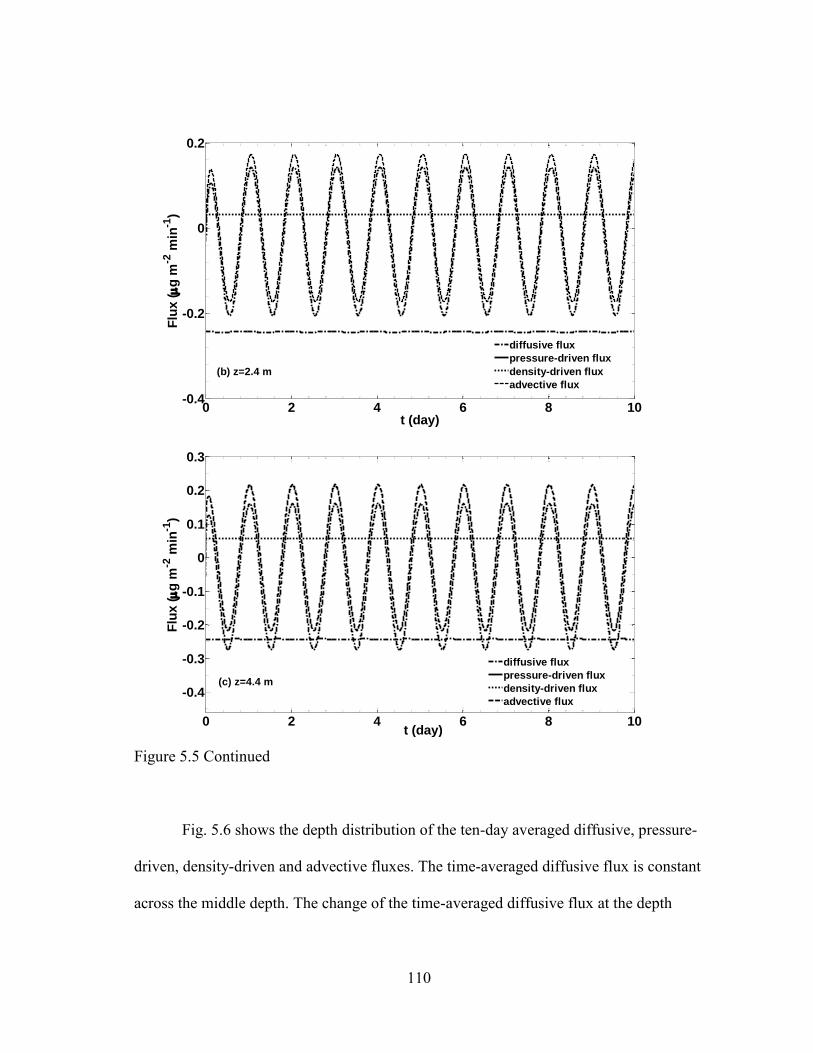
110

0 2 4 6 8 10-0.4

-0.2

0

0.2

t (day)

Flu

x (g

m-2

min

-1)

diffusive flux

pressure-driven flux

density-driven flux

advective flux

(b) z=2.4 m

0 2 4 6 8 10

-0.4

-0.3

-0.2

-0.1

0

0.1

0.2

0.3

t (day)

Flu

x (g

m-2

min

-1)

diffusive flux

pressure-driven flux

density-driven flux

advective flux

(c) z=4.4 m

Figure 5.5 Continued

Fig. 5.6 shows the depth distribution of the ten-day averaged diffusive, pressure-

driven, density-driven and advective fluxes. The time-averaged diffusive flux is constant

across the middle depth. The change of the time-averaged diffusive flux at the depth

111

close to the water table and the ground surface may be caused by the influence of the

atmospheric pressure, water table fluctuations and the boundary conditions on the

transient concentration distribution there. The time-averaged pressure-driven and

density-driven fluxes increase linearly with depth, which is related to the initial

concentration distribution. The magnitude of the time-averaged pressure-driven flux is

close to that of the density-driven flux through the unsaturated zone. Both the net effects

of the diffusive and advective fluxes are to move carbon tetrachloride out of the

-0.2435 -0.2434 -0.2433 -0.24320

1

2

3

4

5

z (

m)

-0.08 -0.06 -0.04 -0.02 00

1

2

3

4

5

0 0.02 0.04 0.06 0.080

1

2

3

4

5

Flux (g m-2

min-1

)

-10 -5 0 5

x 10-4

0

1

2

3

4

5(d)

(b)(a)

(c)

Figure 5.6 Comparison of ten-day averaged (a) diffusive flux, (b) pressure-driven flux, (c) density-driven flux, (d) advective flux. Positive values mean downward fluxes; negative values mean upward fluxes.

unsaturated zone. However, the time averaged diffusive flux is three orders of magnitude

greater than that of advective flux. The maximum advective flux happens at the middle

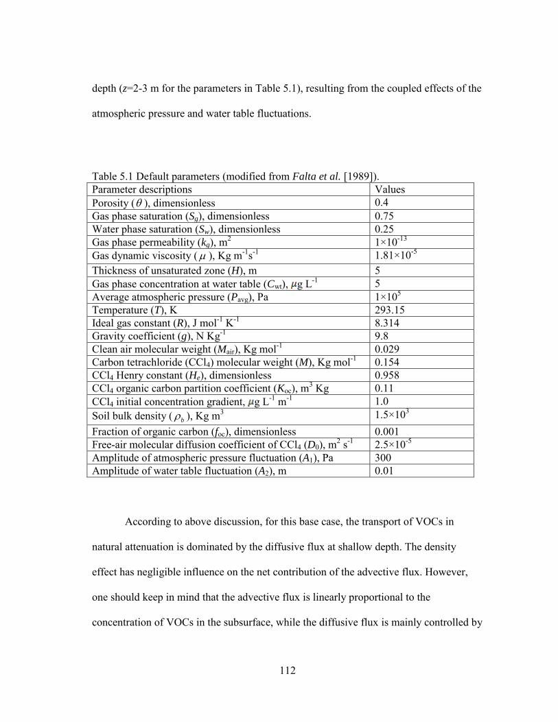
112

depth (z=2-3 m for the parameters in Table 5.1), resulting from the coupled effects of the

atmospheric pressure and water table fluctuations.

Table 5.1 Default parameters (modified from Falta et al. [1989]). Parameter descriptions Values Porosity ( ), dimensionless 0.4 Gas phase saturation (Sg), dimensionless 0.75 Water phase saturation (Sw), dimensionless 0.25 Gas phase permeability (kg), m2 1×10-13 Gas dynamic viscosity ( ), Kg m-1s-1 1.81×10-5 Thickness of unsaturated zone (H), m 5 Gas phase concentration at water table (Cwt), g L-1 5 Average atmospheric pressure (Pavg), Pa 1×105 Temperature (T), K 293.15 Ideal gas constant (R), J mol-1 K-1 8.314 Gravity coefficient (g), N Kg-1 9.8 Clean air molecular weight (Mair), Kg mol-1 0.029 Carbon tetrachloride (CCl4) molecular weight (M), Kg mol-1 0.154 CCl4 Henry constant (He), dimensionless 0.958 CCl4 organic carbon partition coefficient (Koc), m3 Kg 0.11 CCl4 initial concentration gradient, g L-1 m-1 1.0 Soil bulk density ( b ), Kg m3 1.5×103 Fraction of organic carbon (foc), dimensionless 0.001 Free-air molecular diffusion coefficient of CCl4 (D0), m2 s-1 2.5×10-5 Amplitude of atmospheric pressure fluctuation (A1), Pa 300 Amplitude of water table fluctuation (A2), m 0.01

According to above discussion, for this base case, the transport of VOCs in

natural attenuation is dominated by the diffusive flux at shallow depth. The density

effect has negligible influence on the net contribution of the advective flux. However,

one should keep in mind that the advective flux is linearly proportional to the

concentration of VOCs in the subsurface, while the diffusive flux is mainly controlled by

113

the concentration gradient. Therefore, in the case of a uniform distribution of VOCs or

high concentration of VOCs, the advective flux can dominate the transport at the

beginning stage. This conclusion may also change with the field hydrogeological

conditions.

5.4.2 Sensitivity analysis

In this section, we will investigate the dominant transport mechanism of VOCs

under various hydrogeological conditions. The diffusive (qd), pressure-driven (qp) and

density-driven (qg) advective fluxes are calculated by the following equations,

respectively:

z

CDq

g

gd

3.15.2

0 , (5-12)

gg

g

g

g CRT

PM

M

MC

gkq ])1([ airair

, (5-13)

g

g

g

p Cz

Pkq

. (5-14)

According to Eqs. (5-12)-(5-14), the gas-filled porosity and thickness of the unsaturated

zone may influence the magnitudes of all three transport mechanisms. The change of the

gas phase permeability and viscosity could change the magnitudes of the pressure-driven

and density-driven fluxes. Besides these common parameters, pressure-driven flux is

primarily determined by the atmospheric pressure and water table fluctuations. Density-

driven flux is expected to increase with the molecular weight of VOC as well as the

concentration of the VOC. In the following discussion, we neglect the sensitivity

analysis on the gas dynamic viscosity which is temperature-dependent, and detectable

temperature variations usually only exist in the topsoil. When the sensitivity to one

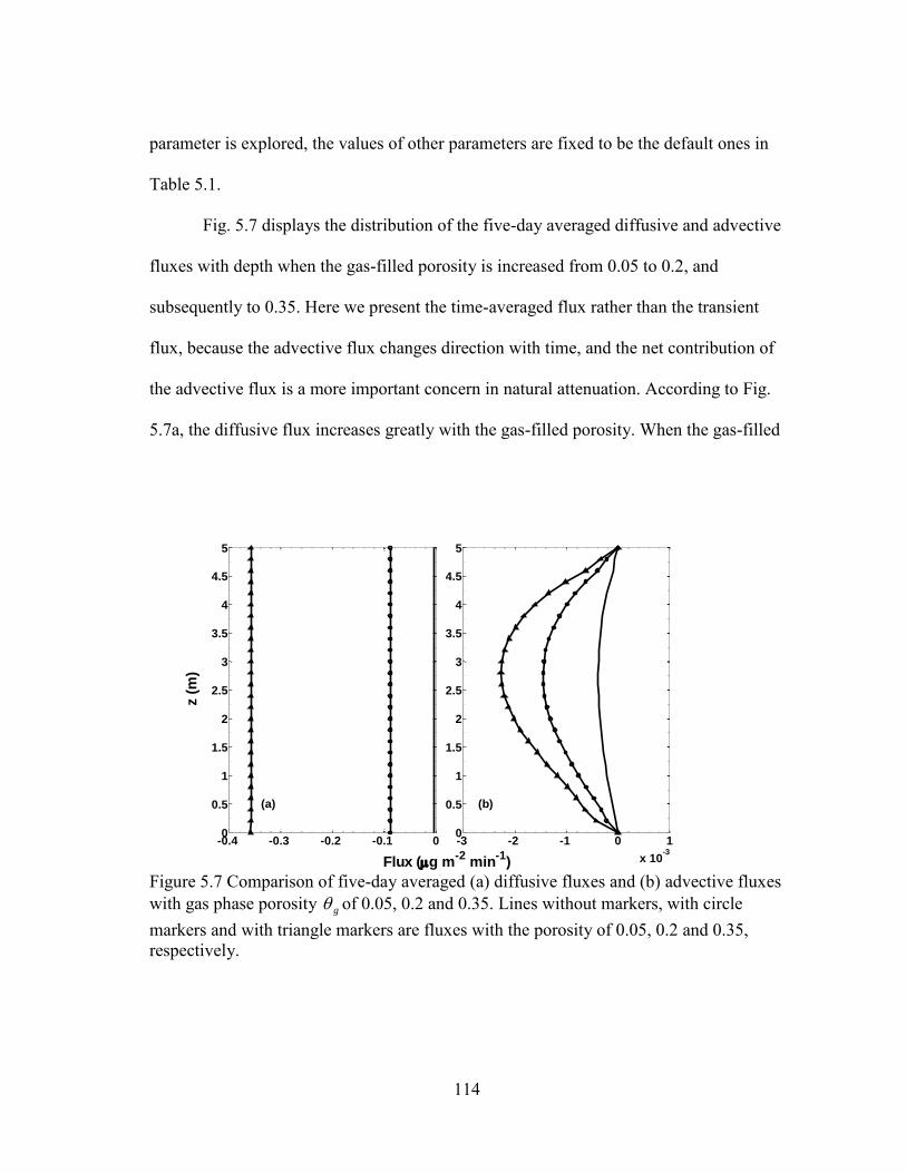
114

parameter is explored, the values of other parameters are fixed to be the default ones in

Table 5.1.

Fig. 5.7 displays the distribution of the five-day averaged diffusive and advective

fluxes with depth when the gas-filled porosity is increased from 0.05 to 0.2, and

subsequently to 0.35. Here we present the time-averaged flux rather than the transient

flux, because the advective flux changes direction with time, and the net contribution of

the advective flux is a more important concern in natural attenuation. According to Fig.

5.7a, the diffusive flux increases greatly with the gas-filled porosity. When the gas-filled

-0.4 -0.3 -0.2 -0.1 00

0.5

1

1.5

2

2.5

3

3.5

4

4.5

5

z (

m)

-3 -2 -1 0 1

x 10-3

0

0.5

1

1.5

2

2.5

3

3.5

4

4.5

5

Flux (g m-2

min-1

)

(b)(a)

Figure 5.7 Comparison of five-day averaged (a) diffusive fluxes and (b) advective fluxes with gas phase porosity g of 0.05, 0.2 and 0.35. Lines without markers, with circle markers and with triangle markers are fluxes with the porosity of 0.05, 0.2 and 0.35, respectively.

115

porosity is 0.05, the averaged diffusive flux is around 3.88 g m-2 day-1, which is

comparable in magnitude with the averaged advective flux. As the gas-filled porosity

increases to 0.2 and 0.35, the time-averaged advective flux also increases. However, its

rate of increase is much slower than that of the diffusive flux. The diffusive flux is about

two orders of magnitude greater than the advective flux in an unsaturated zone with high

gas-filled porosity (greater than 0.2 for the parameters in Table 5.1). The position of the

maximum averaged advective flux remains at the middle depth and does not change with

the gas-filled porosity.

Comparisons of the one-day averaged diffusive and advective fluxes with the

average thickness of the unsaturated zone H increasing from 2.5 m to 15 m, and to 30 m

are presented in Fig. 5.8. According to Fig. 5.8, the diffusive flux slightly changes with

the thickness of the unsaturated zone. However, the advective flux is increased by more

than 20 times in magnitude when H increases from 2.5 m to 15 m. Further increasing H

from 15 m to 30 m does not change the depth averaged magnitude of the advective flux

much. However, the distribution pattern of the advective flux with depth is changed

dramatically because of the attenuation of the pressure wave induced by the atmospheric

pressure and water table fluctuations in the unsaturated zone. The maximum upward

advective fluxes happen at either the deep depth close to the water table or shallow depth

close to the ground surface. At the middle depth (around 15 m), where the influence of

the atmospheric pressure and water table fluctuations is small, the averaged advective

flux is also small.

116

-0.2436 -0.2434 -0.2432 -0.243 -0.24280

0.1

0.2

0.3

0.4

0.5

0.6

0.7

0.8

0.9

1

z/H

-10 -5 0 5

x 10-3

0

0.1

0.2

0.3

0.4

0.5

0.6

0.7

0.8

0.9

1

Flux (g m-2

min-1

)

(a) (b)

Figure 5.8 Comparison of five-day averaged (a) diffusive fluxes and (b) advective fluxes with the average water table depth H of 2.5 m, 15 m and 30 m. Solid lines with markers, solid lines without markers and dashed lines are the fluxes with the average water table depth of 2.5, 15 and 30 m, respectively.

Fig. 5.9 shows the distribution of the five-day averaged advective flux with depth

when the gas phase permeability kg increases from 0.001 to 0.01, 0.1, 1 and 10 Darcys.

As indicated in Eqs. (5-13)-(5-14), the transient advective flux should increase linearly

with kg, however, the time-averaged advective flux is not quite sensitive to kg when its

value is small. As the gas phase permeability increases from 0.001 to 0.01, and 0.1

Darcys, the averaged advective flux slightly increases, and its maximum value shifts

from deep depth (about 4.5 m) to middle depth (about 3.3 m and 2.7 m). Further

increasing the gas phase permeability from 0.1 to 1 and 10 Darcys decreases rather than

increases the time-averaged advective flux across the whole unsaturated zone. This

observation could be explained by the plug flow property of the advective transport.

117

When the gas phase permeability is greater than 1 Darcy, the soil retardation to the

atmospheric pressure and water table fluctuations is small, and the gas flow velocity

induced by them becomes more symmetric in time.

-2.5 -2 -1.5 -1 -0.5 0 0.5

x 10-3

0

1

2

3

4

5

Flux (g m-2

min-1

)

z (

m)

kg=10

-15 m

2

kg=10

-14 m

2

kg=10

-13 m

2

kg=10

-12 m

2

kg=10

-11 m

2

Figure 5.9 Comparison of five-day averaged advective fluxes with gas phase permeability kg of 1.0×10-15 m2, 1.0×10-14 m2, 1.0×10-13 m2, 1.0×10-12 m2 and 1.0×10-11 m2.

In order to investigate the decoupled contribution of the atmospheric pressure

and water table fluctuations to the advective flux, the advective flux is calculated by

setting the water table velocity Vwt to zero in Fig. 5.10 and by fixing the gas pressure at

the ground surface to be the mean atmospheric pressure Pavg in Fig. 5.11. Fig. 5.10

compares the five-day averaged advective flux when the magnitude of the atmospheric

pressure fluctuation A1 is increased from 100 Pa to 300 Pa, 500 Pa, 1000 Pa, and 1500

118

Pa. As evident in Fig. 5.10, the magnitude of the advective flux linearly increases with

A1. However, the averaged diffusive flux (about 350 g m-2 day-1) is still about two

orders of magnitude greater than the averaged advective flux even when the atmospheric

pressure increases by 1500 Pa in 6 hours.

-6 -5 -4 -3 -2 -1 0

x 10-3

0

1

2

3

4

5

Flux (g m-2

min-1

)

z (

m)

A1=100 Pa

A1=300 Pa

A1=500 Pa

A1=1000 Pa

A1=1500 Pa

Figure 5.10 Comparison of five-day averaged advective fluxes with the magnitude of atmospheric pressure fluctuation A1 of 100 Pa, 300 Pa, 500 Pa, 1000 Pa and 1500 Pa.

In Fig. 5.11, we study the five-day averaged advective flux with the magnitude of

the water table fluctuation A2 varying from 0.001 to 0.005, 0.01, 0.05 and 0.1 m. Similar

to the influence of the atmospheric pressure fluctuation, the averaged advective flux

increases linearly with the magnitude of the water table fluctuation. However, when the

magnitude of the water table fluctuation is greater than 0.05 m, the direction of the

averaged advective flux shifts from upward to downward toward water table in deep

119

depth. Our simulation shows that further increasing A2 from 0.1 m would decrease the

advective flux in shallow depth while increase it at deep depths. Besides, the averaged

advective flux slightly decreases with the periods of the atmospheric pressure and water

table fluctuations because of the decreased atmospheric pressure changing rate and water

table moving velocity.

-5 0 5

x 10-3

0

1

2

3

4

5

Flux (g m-2

min-1

)

z (

m)

A2=0.001 m

A2=0.005 m

A2=0.01 m

A2=0.05 m

A2=0.1 m

Figure 5.11 Comparison of five-day averaged advective fluxes with the magnitude of water table fluctuation A2 of 0.001 m, 0.005 m, 0.01 m, 0.05 m and 0.1 m.

We have compared the time-averaged advective fluxes with and without taking

into account the density effect under various conditions. Result indicates that the

density-driven flux can be neglected under usual field conditions. Besides, the

comparisons of the advective transport of TCE and benzene with and without

considering the density effect also show that the density-driven flux is negligible.

120

However, when the concentration gradient of carbon tetrachloride is increased to 100 g

L-1 m-1, neglecting the density-driven flux slightly overestimates the time-averaged

advective flux.

To summarize this section, although the transient advective flux may increase

greatly with the gas phase permeability and the magnitudes of the atmospheric pressure

and water table fluctuations, under most field conditions the time-averaged advective

flux is much less than the diffusive flux, and the influence of the density-driven flux is

undetectable. The time-averaged advective flux is comparable in magnitude with the

diffusive flux only when the gas-filled porosity is less than 0.05 for the parameters listed

in Table 5.1.

5.4.3 VOCs transport in a layered unsaturated zone

In field conditions, the unsaturated zone is usually heterogeneous and may

consist of layers with different soil materials. Even when the soil texture and structure

are homogeneous, the near surface gas-filled porosity and gas phase permeability can be

varied dramatically by the infiltration of water. Therefore, it is important to study VOC

transport in a multilayered unsaturated zone. The transport of VOC in a two-layered

unsaturated zone with different gas-filled porosities and gas phase permeabilities is

investigated as an example. In the following discussion, the relative gas phase

permeability krg (dimensionless) is related to the gas phase saturation Sg by the

expression krg=Sg3 [Falta et al., 1989].

Fig. 5.12 shows the comparisons of the five-day averaged advective and diffusive

fluxes in a homogeneous and a two-layered unsaturated zone. The homogeneous

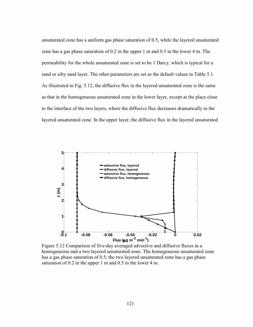
121

unsaturated zone has a uniform gas phase saturation of 0.5, while the layered unsaturated

zone has a gas phase saturation of 0.2 in the upper 1 m and 0.5 in the lower 4 m. The

permeability for the whole unsaturated zone is set to be 1 Darcy, which is typical for a

sand or silty sand layer. The other parameters are set as the default values in Table 5.1.

As illustrated in Fig. 5.12, the diffusive flux in the layered unsaturated zone is the same

as that in the homogeneous unsaturated zone in the lower layer, except at the place close

to the interface of the two layers, where the diffusive flux decreases dramatically in the

layered unsaturated zone. In the upper layer, the diffusive flux in the layered unsaturated

-0.1 -0.08 -0.06 -0.04 -0.02 0 0.020

1

2

3

4

5

Flux (g m-2

min-1

)

z (

m)

advective flux, layered

diffusive flux, layered

advective flux, homogeneous

diffusive flux, homogeneous

Figure 5.12 Comparison of five-day averaged advective and diffusive fluxes in a homogeneous and a two layered unsaturated zone. The homogeneous unsaturated zone has a gas phase saturation of 0.5; the two layered unsaturated zone has a gas phase saturation of 0.2 in the upper 1 m and 0.5 in the lower 4 m.

122

zone is much less than that in the homogeneous unsaturated zone because of the

decreased effective diffusion coefficient. Compared with the averaged advective flux in

the homogeneous unsaturated zone, the averaged advective flux in the layered

unsaturated zone is increased to two times greater in the lower permeable layer (which is

apparent when the advective fluxes are drawn in a figure with a smaller scale) and to one

order of magnitude greater in the upper less permeable layer, where the averaged

advective flux is comparable in magnitude with the averaged diffusive flux. This could

be explained by the increased pressure gradient through the unsaturated zone in the

presence of a less permeable layer (Decreasing the gas permeability increases the soil

retardation to atmospheric pressure wave when it propagates into deep soil, thus,

increases the gas pressure gradient across the unsaturated zone). Therefore, a less

permeable layer at the ground surface is favorable for the removal of VOCs from the

deep unsaturated zone. Under this situation, the advective flux may be comparable with

the diffusive flux in the upper layer.

In Fig. 5.13, we compares the five-day averaged diffusive and advective fluxes in

a homogeneous unsaturated zone with a uniform gas phase saturation of 0.5 and in a

two-layered unsaturated zone with a gas phase saturation of 0.5 in the lower 4 m and 0.8

in the upper 1 m. The other parameters are the same as those in Fig. 5.13. According to

Fig. 5.13, the averaged advective flux in the layered unsaturated zone is slightly

decreased in the lower layer compared with that in the homogeneous unsaturated zone.

In the upper more permeable layer, the magnitude of the averaged advective flux is

significantly increased and the direction is shifted from upward to downward. However,

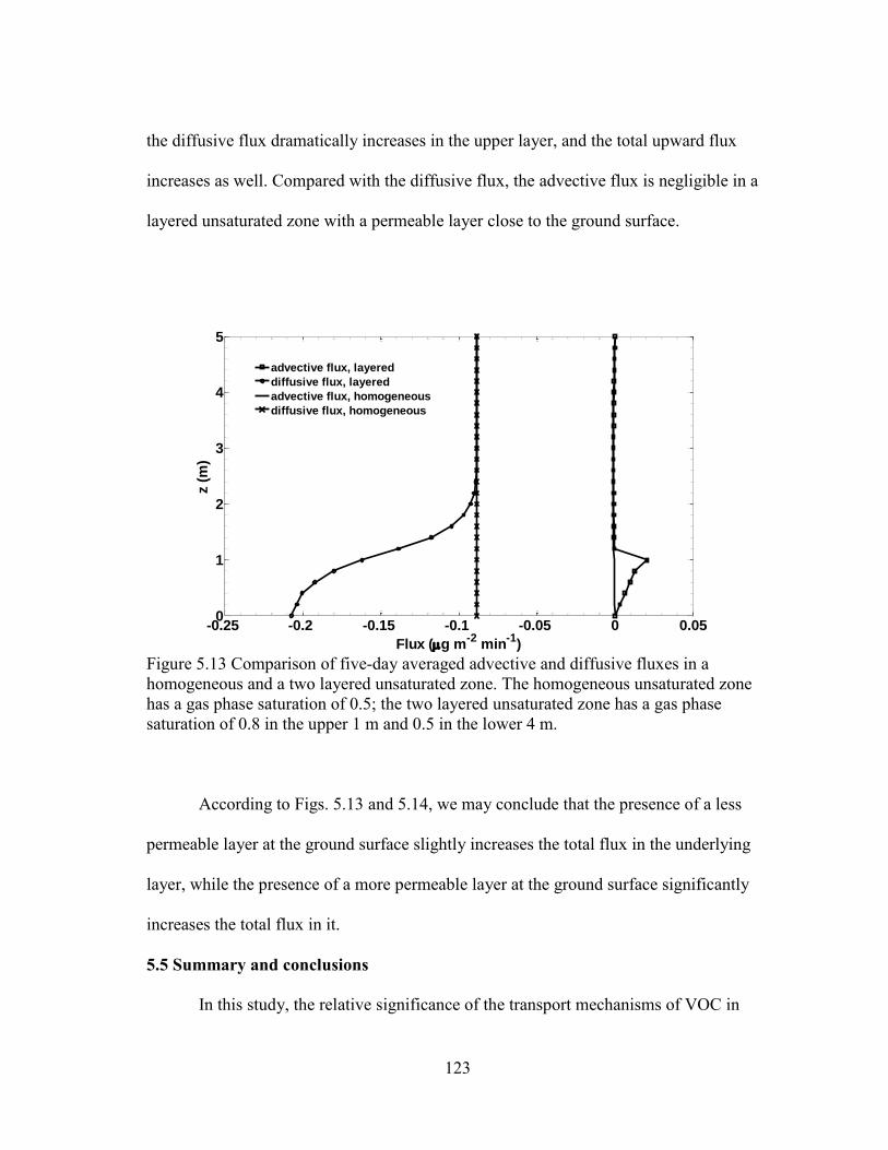
123

the diffusive flux dramatically increases in the upper layer, and the total upward flux

increases as well. Compared with the diffusive flux, the advective flux is negligible in a

layered unsaturated zone with a permeable layer close to the ground surface.

-0.25 -0.2 -0.15 -0.1 -0.05 0 0.050

1

2

3

4

5

Flux (g m-2

min-1

)

z (

m)

advective flux, layered

diffusive flux, layered

advective flux, homogeneous

diffusive flux, homogeneous

Figure 5.13 Comparison of five-day averaged advective and diffusive fluxes in a homogeneous and a two layered unsaturated zone. The homogeneous unsaturated zone has a gas phase saturation of 0.5; the two layered unsaturated zone has a gas phase saturation of 0.8 in the upper 1 m and 0.5 in the lower 4 m.

According to Figs. 5.13 and 5.14, we may conclude that the presence of a less

permeable layer at the ground surface slightly increases the total flux in the underlying

layer, while the presence of a more permeable layer at the ground surface significantly

increases the total flux in it.

5.5 Summary and conclusions

In this study, the relative significance of the transport mechanisms of VOC in

124

unsaturated zones, the diffusive flux, the pressure-driven advective flux and density-

driven advective flux, was investigated under various natural conditions. The pressure-

driven advective flux was induced by the atmospheric pressure and water table

fluctuations. The density-driven advective flux was resulted from the difference of the

molecular weights between VOC and the clean air. The assumption of chemical

equilibrium was employed to relate the concentrations of VOC in the gas phase,

dissolved phase and adsorbed phase. The developed model was applied to interpret a

field study of TCE contamination in the unsaturated zone at Picatinny Arsenal in Morris

County, New Jersey, USA. The time-averaged diffusive flux and advective flux taking

into account or neglecting density effect were compared under various field conditions.

The presence of a less or more permeable layer at the ground surface in a layered

unsaturated zone, and the assumption of a fixed water table position but fluctuating

water table moving velocity were investigated.

The following conclusions can be drawn from the numerical model for the field

conditions discussed in this study:

1. Although the transient advective flux may increase greatly with the gas-phase

permeability and the magnitudes of the atmospheric pressure and water table fluctuations,

under most of the field conditions the time-averaged advective flux is one to three orders

of magnitude less than the diffusive flux, and the influence of the density-driven flux is

undetectable.

2. The time-averaged diffusive flux increases dramatically with the gas-filled

porosity, while the time-averaged advective flux increases linearly with the magnitudes

125

of the atmospheric pressure and water table fluctuations. For the parameters we used in

this study, increasing the thickness of the unsaturated zone from 2.5 m to 15 m

dramatically increases the time-averaged advective flux. The time-averaged advective

flux is comparable in magnitude with the diffusive flux when the gas-filled porosity is

less than 0.05. Both are relatively insignificant at that porosity.

3. The presence of a less permeable layer at the ground surface slightly increases

the total flux in the underlying layer; under this condition, the time-averaged advective

flux is comparable with the diffusive flux in the less permeable layer and cannot be

neglected. The presence of a more permeable layer at the ground surface significantly

increases the total flux in it; under this condition, the contribution of the advective is

negligible compared with the diffusive flux.

126

6. SUMMARY AND CONCLUSIONS

6.1 Summary and conclusions

In this dissertation, we investigated the influence of atmospheric pressure and

water table fluctuations on the gas phase flow and transport of VOCs in unsaturated

zones under various hydrogeological conditions.

Attention in active SVE in previous studies was mainly focused on gas flow

induced by active gas injection or pumping, and the atmospheric pressure and water

table fluctuations were neglected. To investigate their influences, a new 2-D

axisymmetric semi-analytical solution was developed by setting the time-dependent

atmospheric pressure in the upper boundary condition and integrating the fluctuating

water table moving velocity in the lower boundary condition. The gas pressure

distribution, the pore-gas velocity and the ROIs for gas pumping wells calculated by

solutions considering and neglecting the atmospheric pressure and water table

fluctuations were compared at both coastal and non-coastal sites under various

hydrogeological conditions.

Atmospheric pressure fluctuation is the driving force in BP. New semi-analytical

solutions were developed to study the subsurface gas flow field and the gas flow rate

to/from a BPW with and without a check valve installed in both homogeneous and

multi-layered unsaturated zones. ROIs and the controlling pressure to open/close check

valves were analyzed to provide guidance for field operations of BP. The solution for BP

in a homogenous unsaturated zone was applied to interpret the field experiment at the

127

A/M area of the Savannah River site in Aiken, South Carolina, and the solution for a

multi-layered unsaturated zone was applied to interpret the field experiment at the

Hanford site in Richland, Washington.

Under natural conditions, the gas phase VOCs in the unsaturated zone can be

transported by the diffusive flux, density-driven advective flux and pressure-driven

advective flux induced by atmospheric pressure and water table fluctuations. A

comprehensive investigation of their relative significance was conducted based on a

newly developed finite difference numerical solution under various hydrogeological

conditions. The presence of a less or more permeable layer at the ground surface in a

multilayered unsaturated zone is investigated for their influence on the time-averaged

advective and diffusive fluxes. From these studies, the following conclusions can be

drawn:

1. The water table effect is negligible but the atmospheric pressure effect is non-

negligible for accurate interpretation of subsurface gas pressure in active SVE in a non-

coastal site where the daily water table fluctuation is in centimeters scale; both the water

table and atmospheric pressure fluctuations need to be considered in a coastal site where

the daily water table fluctuation is in tens of centimeters scale. The errors induced from

neglecting their effects are amplified when the atmospheric pressure is increasing and

the water table is moving upward simultaneously, or when the atmospheric pressure is

decreasing and the water table is moving downward simultaneously. Atmospheric

pressure fluctuation mainly impact the ROIs for gas pumping wells defined by the 0.01

cm/s pore-gas velocity contours at the shallow depth. When the atmospheric pressure is

128

higher than its averaged value, the ROIs increase at the shallow depth, and vice versa.

The water table fluctuation changes the ROIs for the gas pumping wells across the whole

unsaturated zone. A downward moving water table increases the ROIs. However, it leads

to greater vertical pore-gas velocity away from the gas pumping well under the well,

which is unfavorable for removing VOCs. Less vertical gas permeability leads to greater

atmospheric pressure and water table effects.

2. The gas flow rate to/from a BPW can be accurately calculated by our newly

developed semi-analytical solutions in both homogeneous and multilayered unsaturated

zones. The ROI for the BPW is time-dependent. It increases with the radial gas

permeability, the gas-filled porosity, the well screen length, and the well depth if the

well depth is small, and decreases with the vertical gas permeability.

3. Although the transient advective flux may increase greatly with the gas-phase

permeability and the magnitudes of the atmospheric pressure and water table fluctuations,

under most of the field conditions the time-averaged diffusive flux is one to three orders

of magnitude greater than the advective flux, and the density-driven flux is negligible.

The time-averaged advective flux is comparable in magnitude with the diffusive flux

only when the gas-filled porosity is very small (less than 0.05). The presence of a less

permeable layer at the ground surface slightly increases the total flux of VOCs in the

underlying layer, while the presence of a more permeable layer at the ground surface

significantly increases the total flux in this layer.

6.2 Contributions

The contribution of this study can be summarized as follows:

129

1. This dissertation for the first time systematically investigated the influence of

the two very important natural dynamic processes on the gas flow in the unsaturated

zone: the atmospheric pressure fluctuation and the water table fluctuation. Rigorous

semi-analytical solutions were for the first time developed to study the gas flow behavior

in BP in both homogeneous and multilayered unsaturated zones. The transport

mechanisms of gas phase VOCs in the unsaturated zone were for the first time

comprehensively analyzed and compared under various natural conditions.

2. This study provides several analytical and semi-analytical solutions for gas

phase flow of VOCs in the subsurface, which can be used to check the accuracy of

numerical solutions. These solutions also provide easy and fast ways to characterize the

unsaturated zone, to do initial site investigation, and to evaluate and optimize the

contaminant remediation techniques.

3. The developed solutions in this study could be extended to investigate the gas

flow in porous and fractured media induced by oscillatory pressures. This study also has

potential application in radon intrusion into surface buildings, nuclear waste storage site

evaluation, plant root respiration, and soil moisture redistribution.

6.3 Future work

Up to now, most of the studies on the transport and fate of VOCs in the

subsurface are process-based, including the study in this dissertation. In the future work,

the simultaneous generation, transport and attenuation of VOCs in the subsurface would

be integrally studied. The influence of the capillary fringe on the mass transfer between

the saturated and unsaturated zones, and the fully coupled fluid flow and heat transport

130

in the unsaturated zone will be investigated. The developed models would be

programmed with a user-friendly window to provide researchers with convenience tools

for evaluating the transport and fate of VOCs and to provide practitioner with guidance

for contaminant remediations. Besides, laboratory studies would be conducted to

explore the details in VOCs transport process and to check and improve the accuracy of

previous modeling studies. Phase equilibrium assumptions for solid, water, and gas

phase VOCs during transport would be reevaluated, and the lumped parameters in the

existing transient mass transfer theory among each phase would be parameterized.

131

REFERENCES

Abriola, L. M. (1989), Modeling multiphase migration of organic chemicals in

groundwater systems-a review and assessment, Environ. Health Persp., 83, 117-

143.

Armstrong, J. E., E. O. Frind, and R. D. McClellan (1994), Nonequilibrium mass

transfer between the vapor, aqueous, solid phase in unsaturated soils during vapor

extraction, Water Resour. Res., 30(2), 355-368, doi:10.1029/93WR02481.

Auer, L. H., N. D. Rosenberg, K. H. Birdsell, and E. M. Whitney (1996), The effects of

barometric pumping on contaminant transport, J. Contam. Hydrol., 24(2), 145-166,

doi:10.1016/S0169-7722(96)00010-1.

Baehr, A. L., and M. F. Hult (1991), Evaluation of unsaturated zone air permeability

through pneumatic tests, Water Resour. Res., 27, 2605-2617.

Baehr, A. L., and R.J. Baker (1995), Use of a reactive gas transport model to determine

rates of hydrocarbon biodegradation in unsaturated porous media, Water Resour.

Res., 31(11), 2877-2882, doi:10.1029/95WR02077.

Baehr, A. L., and C. J. Joss (1995), An updated model of induced air-flow in the

unsaturated zone, Water Resour. Res., 31, 417-421.

Batterman, S. A., B. C. Mcquown, P. N. Murthy, and A. R. Mcfarland (1992), Design

and evaluation of a long-term soil gas flux sampler, Environ. Sci. Technol., 26(4),

709-714, doi:10.1021/es00028a007.

132

Bassani, J. L., M. W. Nansteel, and M. November (1987), Adiabatic-isothermal mixed

boundary conditions in heat transfer, Int. J. Heat Mass Transfer, 30(5), 903-909, doi:

10.1016/0017-9310(87)90009-3.

Butler, J. J., Jr., G. J. Kluitenberg, D. O. Whittemore, S. P. Loheide , II, W. Jin, M. A.

Billinger, et al. (2007), A field investigation of phreatophyte-induced fluctuations in

the water table, Water Resour. Res., 43, W02404, doi: 10.1029/2005WR004627.

Carslaw, H. S., and J. C. Jaeger (1959), Conduction of Heat in Solids, Clarendon Press,

Oxford, U. K..

Cassiani, G., and Z. J. Kabala (1998), Hydraulics of a partially penetrating well: solution

to a mixed-type boundary value problem via dual integral equations, J. Hydrol.,

211(1-4), 100-111, doi: 10.1016/S0022-1694(98)00223-6.

Chang, C. C., and C. S. Chen (2002), An integral transform approach for a mixed

boundary problem involving a flowing partially penetrating well with infinitesimal

well skin, Water Resour. Res., 38(6), 1071, doi:10.1029/2001wr001091.

Chang, C. C., and C. S. Chen (2003), A flowing partially penetrating well in a finite-

thickness aquifer: a mixed-type initial boundary value problem, J. Hydrol., 271(1-4),

101-118, doi:10.1016/S0022-1694(02)00323-2.

Chang, Y. C., and H. D. Yeh (2009), New solutions to the constant-head test performed

at a partially penetrating well, J. Hydrol., 369 (1-2), 90-97, doi:

10.1016/j.jhydrol.2009.02.016.

Chapman, S., and R. L. Lindzen (1970), Atmospheric Tides: Thermal and Gravitational,

Gordon and Breach, New York.

133

Chen, C., R. E. Green, D. M. Thomas, and J. A. Knuteson (1995), Modeling 1,3-

dichloropropene fumigant volatilization with vapor-phase advection in the soil

profile, Environ. Sci. Technol., 29(7), 1816-1821, doi:10.1021/es00007a019.

Chiao, F. F., R. C. Currie, and T. E. McKone (1994), Intermedia transfer factors for

contaminants found at hazardous waste sites trichloroethylene,

http://www.dtsc.ca.gov/AssessingRisk/Upload/pce.pdf.

Cho, H. J., P. R. Jaffe, and J. A. Smith (1993), Simulating the volatilization of solvents

in unsaturated soils during laboratory and field infiltration experiments, Water

Resour. Res., 29(10), 3329-3342, doi:10.1029/93WR01414.

Cho, J. S., and D. C. Digiulio (1992), Pneumatic pumping test for soil vacuum extraction,

Environmental Progress, 11(3), 228-233, doi:10.1002/ep.670110319.

Choi, J. W., F. D. Jr. Tillman, and J. A. Smith (2002), Relative importance of gas-phase

diffusive and advective trichloroethylene (TCE) fluxes in the unsaturated zone

under natural conditions, Environ. Sci. Technol., 36(7), 3157-3164, doi:

10.1021/es950610c.

Choi, J. W., and J. A. Smith (2005), Geoenvironmental factors affecting organic vapor

advection and diffusion fluxes from the unsaturated zone to the atmosphere under

natural condition, Environ. Eng. Sci., 22(1), 95-108, doi:10.1089/ees.2005.22.95.

Conant, B. H., R. W. Gillham, and C. A. Mendoza (1996), Vapor transport of

trichloroethylene in the unsaturated zone: Field and numerical modeling

investigations, Water Resour. Res., 32(1), 9-22, doi:10.1029/95WR02965.

Churchill, R. V. (1958), Operational Mathematics, McGraw-Hill, New York.

134

DiGiulio, D. C., and R. Varadhan (2001), Development of recommendations and

methods to support assessment of soil venting performance and closure, EPA/600/R-

01/070, U.S. Environmental Protection Agency, Cincinnati, Ohio.

Dixon, K. L., and R. L. Nichols (2005), Permeability estimation from transient vadose

zone pumping tests in shallow coastal-plain sediments, Environ. Geosci., 12(4), 279-

289, doi:10.1306/eg.06070505004.

Dixon, K. L., and R. L. Nichols (2006), Soil vapor extraction system design: A case

study comparing vacuum and pore-gas velocity cutoff criteria, Rem. J., 17(1), 55-67,

doi: 10.1002/rem.20112

Ellerd, M. G., J. W. Massmann, D. P. Schwaegler, and V. J. Rohay (1999),

Enhancements for passive vapor extraction: the Hanford study, Ground Water,

37(3), 427-437, doi: 10.1111/j.1745-6584.1999.tb01122.x.

Falta, R. W. (1995), A program for analyzing transient and steady-state soil gas pump

tests, Ground Water, 34(4), 750-755.

Falta, R. W., I. Javandel, K. Pruess, and P. A. Witherspoon (1989), Density-driven flow

in gas in the unsaturated zone due to the evaporation of volatile organic compounds,

Water Resour. Res., 25(10), 2159-2169, doi:10.1029/WR025i010p02159.

Fletcher, C. A. J. (1991), Computational Techniques for Fluid Dynamics, Volume. 1:

Fundamental and General Techniques, 2nd ed., Springer, New York.

Frank, U., and N. Barkley (1995), Remediation of low permeability subsurface

formations by fracturing enhancement of soil vapor extraction, J. Hazardous

Materials, 40(2), 191-201, doi:10.1016/0304-3894(94)00069-S.

135

Freeze, R. A., and J. A. Cherry (1979), Groundwater, Prentice-Hall, Englewood Cliffs,

New York.

Gurdak, J. J., R. T. Hanson, P. B. McMahon, B. W. Bruce, J. E. McCray, G. D. Thyne,

et al. (2007), Climate variability controls on unsaturated water and chemical

movement, High Plains aquifer, USA, Vadose Zone J., 6(3), 533-547,

doi:10.2136/vzj2006.0087.

Hantush, M. S. (1964), Hydraulics of wells, Adv. Hydrosci., 1, 281-432.

Hollenbeck, K. J. (1998), INVLAP. M: A Matlab function for numerical inversion of

Laplace transforms by the de Hoog algorithm,

http://www.isva.dtu.dk/staff/karl/invlap.htm.

Huang, S. C., and Y. P. Chang (1984), Anisotropic heat conduction with mixed

boundary conditions, J. Heat Transfer, 106, 646-648.

Jacob, C. E. (1946), Radial flow in a leaky artesian aquifer, Trans. Amer. Geophys.

Union, 27, 198-205.

Jennings, A. A., and P. Patil (2002), Feasibility modeling of passive soil vapor extraction,

J. Environ. Engineer. Sci., 1(16), 157-172.

Jiao, J., and H. Li (2004), Breathing of coastal vadose zone induced by sea level

fluctuations, Geophys. Res. Lett., 31, L11502, doi:10.1029/2004GL019572.

Kamath, R., D. T. Adamason, and C. J. Newell (2009), Passive soil vapor extraction,

DE-AC09-08SR22470, U. S. Department of Energy, Aiken, South Carolina.

Karimi, A. A., W. J. Farmer, and M. M. Cliath (1987), Vapor-phase diffusion of benzene

in soil, J. Environ. Qual., 16(1), 38-43.

136

Khan, F. I., T. Husain, and R. Hejazi (2004), An overview and analysis of site

remediation technologies, J. Environ. Manage., 71(2), 95-122, doi:

10.1016/j.jenvman.2004.02.003.

Lapidus, L., and N. R. Amundson (1952), Mathematics of adsorption in beds. VI. The

effect of longitudinal diffusion in ion exchange and chromatographic columns, J.

Phys. Chem., 56(8), 984-988, doi:10.1021/j150500a014.

Li, H., and J. Jiao (2005), One-dimensional airflow in unsaturated zone induced by

periodic water table fluctuation, Water Resour. Res., 41, W04007,

doi:10.1029/2004WR003916.

Li, J., H. Zhan, G. Huang, and K. You (2011), Tide-induced airflow in a two-layered

coastal land with atmospheric pressure fluctuations, Adv. Water Resour., 34(5), 649-

658, doi:10.1016/j.advwatres.2011.02.014.

Li, J., H. Zhan, G. Huang, and K. You (2012), Analytical solution to subsurface air

pressure in a three-layer unsaturated zone with atmospheric pressure changes, Transp.

Porous Med., 93, 461-474, doi:10.1007/s11242-012-9964-5 .

Lee, C. H., J. Y. Lee, W. Y. Jang, Y. H. Jeon, and K. K. Lee (2002), Evaluation of air

injection and extraction tests as a petroleum contaminated site, Korea, Water, Air,

Soil Pollut., 135(1-4), 65-91, doi: 10.1023/A:1014772324881.

Lowry, W., S. D. Dunn, and D. Neeper (1995), Barometric pumping with a twist: VOC

contaminated and remediation without boreholes, in Environmental Technology

Development Through Industry Partnership, Morgantown, West Virginia.

137

Marrin, D. L., and G. M. Thompson (1987), Gaseous behavior of TCE overlying a

contaminated aquifer, Ground Water, 25(1), 21-27, doi:10.1111/j.1745-

6584.1987.tb02112.x.

Marrin, D. L., and H. B. Kerfoot (1988), Soil-gas surveying techniques, Environ. Sci.

&Technol., 22(7), 740-745, doi:10.1021/es00172a001.

Massman, W. J. (2006), Advective transport of CO2 in permeable media induced by

atmospheric pressure fluctuations: 1. An analytical model, J. Geophys. Res., 111,

G03004, doi:10.1029/2006JG000163.

Massmann, J. W. (1989), Applying groundwater flow models in vapor extraction system

design, J. Environ. Eng., 115(1), 129-149, doi:10.1061/(ASCE)0733-9372.

Massmann, J., and D. F. Farrier (1992), Effects of atmospheric pressures on gas

transport in the vadose zone, Water Resour. Res., 28(3), 777-791,

doi:10.1029/91WR02766.

Mendoza, A. C., and E. O. Frind (1990a), Advective-dispersive transport of dense

organic vapors in the unsaturated zone 1. Model development, Water Resour. Res.,

26(3), 379-387, doi:10.1029/WR026i003p00379.

Mendoza, A. C., and E. O. Frind (1990b), Advective-dispersive transport of dense

organic vapors in the unsaturated zone 2. Sensitivity analysis, Water Resour. Res.,

26(3), 388-398, doi:10.1029/WR026i003p00388.

Miller, A., and J. C. Thompson(1970), Elements of Meteorology, Merrill, Columbus,

Ohio.

138

Murdoch, L. C. (2000), Remediation of organic chemicals in the vadose zone, in Vadose

Zone, Science and Technology Solutions, edited by B. B. Looney and R. W. Falta,

pp. 949-1327, Battelle Press, Columbus, Ohio.

Neeper, D. A. (2003), Harmonic analysis of flow in open boreholes due to barometric

pressure cycles, J. Contam. Hydrol., 60(3-4), 135-162, doi: 10.1016/So169-

7722(02)00086-5.

Nielsen, P. (1990), Tidal dynamics of the water table in beaches, Water Resour. Res.,

26(9), 2127-2134, doi:10.1029/WR026i009p02127.

Nilson, R. H., E. W. Peterson, K. H. Lie, N. R. Burkhard, and J. R. Hearst (1991),

Atmospheric pumping: a mechanism causing vertical transport of contaminated

gases through fractured permeable media, J. Geophys. Res., 96(B13), 21933-21948,

doi:10.1029/91jb01836.

Noble, B. (1958), Methods Based on the Wiener-Hopf Techniques, Pergamon Press,

New York.

Pirkle, R. J., D. E. Wyatt, V. Price, and B. B. Looney (1992), Barometric pumping: the

connection between the vadose zone and the atmosphere, Ground Water Manag.,

13, 427-439.

Press, W. H., S. A. Teukolsky, W. T. Vetterling, and B. P. Flannery (2007), Numerical

Recipes: the Art of Scientific Computing, 3rd ed., Cambridge University Press, New

York.

139

Raubenheimer, B., R. T. Guza, and S. Elgar (1999), Tidal water table fluctuations in a

sandy ocean beach, Water Resour. Res., 35(8), 2313-2320,

doi:10.1029/1999WR900105.

Riha, B. D. (2005), Passive soil vapor extraction (PSVE) for VOC remediation at the

metallurgical laboratory (MetLab) June 2005 progress report, DE-AC09-96SR18500,

U. S. Department of Energy, Aiken, South Carolina.

Rivett, M. O., G. P.Wealthall, R. A. Dearden, and T. A. McAlary (2011), Review of

unsaturated-zone transport and attenuation of volatile organic compound (VOC)

plumes leached from shallow source zones, J. Contam. Hydrol., 123, 130-156.

Rohay, V. J., J. Rossabi, B. Looney, R. Cameron, and B. Peters (1993), Well venting and

application of passive soil vapor extraction at Hanford and Savannah River, ER 93

Environmental Remediation Conference, August, Georgia.

Rohay, V. J., R. J. Cameron, B. B. Peters, J. Rossabi, B. D. Riha, and W. Downs (1997),

Passive soil vapor extraction, BHI-01089, the office of Environmental Restoration, U.

S. Department of Energy.

Rossabi, J., B. B. Looney, C.A.E. Dilek, B. R. Orise, and V. J. Rohay (1993), Passive

remediation of chlorinated volatile organic compounds using barometric pumping,

WSRC –MS-93-615, U. S. Department of Energy.

Rossabi, J. (1999), The influence of atmospheric pressure variations on subsurface soil

gas and the implications for environmental characterization and remediation, Ph.D.

Dissertation, Alabama, Clemson University.

140

Rossabi, J., and R. W. Falta (2002), Analytical solutions for subsurface gas flow to a

well induced by surface pressure fluctuations, Ground Water, 40(1), 67-75.

Rossabi, J. (2006), Analyzing barometric pumping to characterize subsurface

permeability, in Gas Transport in Porous Media, edited by C. K. Ho and S. W.

Webb, pp. 279-290, Springer, Dordrecht, Netherlands.

Shan, C. (1995), Analytical solutions for determining vertical air permeability in

unsaturated soils, Water Resour. Res., 31(9), 2193-2200, doi:10.1029/95WR01653.

Shan, C., I. Javandel, and P. A. Witherspoon (1999), Characterization of leaky faults:

Study of air flow in faulted vadose zones, Water Resour. Res., 35(7), 2007-2013,

doi:10.1029/1999WR900037.

Shan, C., R. W. Falta, and I. Javandel (1992), Analytical solutions for steady state gas

flow to a soil vapor extraction well, Water Resour. Res., 28(4), 1105-1120,

doi:10.1029/91WR02986.

Sleep, B. E., and J. F. Sykes (1989), Modeling the transport of volatile organics in

variably saturated media, Water Resour. Res., 25(1), 81-92,

doi:10.1029/WR025i001p00081.

Smith, J. A., A. K. Tisdale, and H. J. Cho (1996), Quantification of natural vapor fluxes

of trichloroethylene in the unsaturated zone at Picatinny Arsenal, New Jersey,

Environ. Sci. Technol., 30(7), 2243-2250, doi:10.1021/es950610c.

Smith, J. A., C. T. Chiou, J. A. Kammer, and D. E. Kile (1990), Effect of soil moisture

on the sorption of trichloroethylene vapor to vadose-zone soil at Picatinny Arsenal,

New Jersey, Environ. Sci. Technol., 24(5), 676-683.

141

Sneddon, I. N. (1996), Mixed Boundary Value Problems in Potential Theory, North-

Holland Pub. Co., Amsterdam and New York.

Switzer, C., and D. S. Kosson (2007), Evaluation of air permeability in layered

unsaturated materials, J. Contam. Hydrol., 90(3-4), 125-145,

doi:10.1016/j.jconhyd.2005.09.008.

Thorstenson, D. C., and D. W. Pollock (1989), Gas transport in unsaturated zones:

Multicomponent systems and the adequacy of Fick's laws, Water Resour. Res.,

25(3), 477–507, doi:10.1029/WR025i003p00477.

Turk, L. J. (1975), Diurnal fluctuations of water tables induced by atmospheric pressure

changes, J. Hydrol., 26(1-2), 1-16, doi: doi.org/10.1016/0022-1694(75)90121-3.

US Environmental Protection Agency (EPA) (1994), How to evaluate alternative

cleanup technologies for underground storage tank sites: a guide for corrective

action plan reviewers, http://www.epa.gov/oust/pubs/tums.htm.

Vangelas, K., B. Looney, R. Kamath, D. Adamson, and C. Newell (2010), Enhanced

attenuation technologies: Passive soil vapor extraction, DE-AC09-08SR22470, U.S.

Department of Energy, Aiken, South Carolina.

Van Genuchten, M. T., and J. C. Parker (1984), Boundary conditions for displacement

experiments through short laboratory soil columns, Soil Sci. Soc. AM. J., 48(4),

703-708.

Wetherold, R. G., B. M. Eklund, B. L. Blaney, and S. A. Thorneloe (1986), Assessment

of volatile organic emissions from a petroleum refinery land treatment site,

EPA/600/D-86/074, U.S. Environmental Protection Agency, Washington, DC.

142

Wilkinson, D., and P. S. Hammond (1990), A perturbation method for mixed boundary

value problems in pressure transient testing, Transp. Porous Med., 5(6), 609-636,

doi:10.1007/BF00203331.

Yedder, R. B., and E. Bilgen(1994), On adiabatic-isothermal mixed boundary conditions

in heat transfer, Heat Mass Transfer, 29(7), 457-460, doi:10.1007/BF01584048.

You, K., and H. Zhan (2012), Can atmospheric pressure and water table fluctuation be

neglected in soil vapor extraction? Adv. Water Resour., 35, 41-54,

doi:10.1016/j.advwatres.2011.10.008.

You, K., and H. Zhan (2013), Comparisons of diffusive and advective fluxes of gas

phase volatile organic compounds (VOCs) in unsaturated zones under natural

conditions, Adv. Water Resour., 52, 221-231.

You, K., H. Zhan, and J. Li (2010), A new solution and data analysis for gas flow to a

barometric pumping well, Adv Water Resour., 33(12), 1444-1455, doi:

10.1016/j.advwatres.2010.07.008.

You, K., H. Zhan, and J. Li (2011a), Gas flow to a barometric pumping well in a

multilayered unsaturated zone, Water Resour. Res., 47, W05522,

doi:10.1020/2010WR009411R.

You, K., H. Zhan, and J. Li (2011b), Analysis of models for induced gas flow in the

unsaturated zone, Water Resour. Res., 47, W04515, doi:10.1029/2010WR009985.

Zhan, H., and E. Park (2002), Vapor flow to horizontal wells in unsaturated zones, Soil

Sci. Soc. Am. J., 66(3), 710-721, doi: 10.2136/sssaj2002.7100.

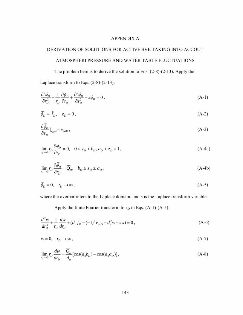
143

APPENDIX A

DERIVATION OF SOLUTIONS FOR ACTIVE SVE TAKING INTO ACCOUT

ATMOSPHERI PRESSURE AND WATER TABLE FLUCTUATIONS

The problem here is to derive the solution to Eqs. (2-8)-(2-13). Apply the

Laplace transform to Eqs. (2-8)-(2-13):

012

2

2

2

D

D

D

D

D

DD

D szrrr

, (A-1)

0, DDD zf , (A-2)

Dz

D

D vz D wt1|

, (A-3)

1,0,0lim0

DDDD

D

DD

rzabz

rr

D

, (A-4a)

DDDD

D

DD

razbQ

rr

D

,lim

0

, (A-4b)

DD r,0 , (A-5)

where the overbar refers to the Laplace domain, and s is the Laplace transform variable.

Apply the finite Fourier transform to zD in Eqs. (A-1)-(A-5):

22

wt2

1 ( ( 1) ) 0n

n D D n

D D D

d w dwd f v d w sw

dr r dr , (A-6)

Drw ,0 , (A-7)

)]cos()[cos(lim0 DnDn

n

D

D

Dr

adbdd

Q

dr

dwr

D

, (A-8)

144

where )5.0( ndn ; n are positive integers; w is the finite Fourier transform of D

and is expressed as dzznw D ])5.0sin[(1

0 .

The solution to Eqs. (A-6)-(A-8) is:

sd

vfdrsdKbdad

d

Qw

n

D

n

DnDnDnDn

n

D

2

wt20

)1()()]cos()[cos( , (A-9)

where K0 is the zeroth-order modified Bessel Function of the second kind.

The inverse finite Fourier transform of Eq. (A-9) gives the solution to Eqs. (2-8)-

(2-13) in Laplace space as:

)sin()1()()]cos()[cos(21

2wt2

0 Dn

n n

D

n

DnDnDnDn

n

DD zd

sd

vfdrsdKbdad

d

Q

.

(A-10)