inflation persistence in brazil - a cross country comparison
TRANSCRIPT

WP/14/55
Inflation Persistence in Brazil - A Cross
Country Comparison
Shaun K. Roache

© 2013 International Monetary Fund WP/14/55
IMF Working Paper
Western Hemisphere Department
Inflation Persistence in Brazil - A Cross Country Comparison
Prepared by Shaun K. Roache1
Authorized for distribution by Alejandro Santos
April 2014
Abstract
Inflation persistence is sometimes defined as the tendency for price shocks to push the
inflation rate away from its steady state—including an inflation target—for a prolonged
period. Persistence is important because it affects the output costs of lowering inflation
back to the target, often described as the “sacrifice ratio”. In this paper I use inflation
expectations to provide a comparison of inflation persistence in Brazil with a sample of
inflation targeting (IT) countries. This approach suggests that inflation persistence
increased in Brazil through early 2013, in contrast to many of its IT peers, mainly due to
“upward” persistence. The 2013 rate hiking cycle may have contributed to some recent
decline in persistence.
JEL Classification Numbers: E31, E32, P22
Keywords:
Author’s E-Mail Address:[email protected]
1 This paper draws heavily on the Selected Issues Paper from Brazil’s 2013 Article IV Consultation. I would like to
thank seminar participants from the Banco Central do Brasil and Ministério da Fazenda, Martin Kaufman,
Mercedes Garcia-Escribano, Fei Han, and Heedon Kang for helpful comments and suggestions. The usual
disclaimer applies.
This Working Paper should not be reported as representing the views of the IMF.
The views expressed in this Working Paper are those of the author(s) and do not necessarily
represent those of the IMF or IMF policy. Working Papers describe research in progress by the
author(s) and are published to elicit comments and to further debate.

I. INTRODUCTION
Inflation persistence is sometimes defined as the tendency for price shocks to push the
inflation rate away from its steady state—including an inflation target—for a prolonged
period. Persistence is important because it affects the output costs of lowering inflation back
to the target, often described as the “sacrifice ratio”. Equivalently, the lower is persistence
the greater is “policy space,” defined as the ability of monetary policy to accommodate
temporary price shocks. Countries with high persistence and low policy space may need to
adjust macroeconomic policies in a material way to price shocks given that they influence
overall inflation and inflation expectations for a sustained period.
This is a reduced form interpretation of persistence and does not provide a structural
explanation. Persistence may change due to a number of structural reasons, including: inertia
in the underlying “driving process,” such as marginal costs or the output gap; the
policymaker’s reaction function to price or output shocks; and inertia intrinsic to the inflation
process itself, including indexation by price-setters. Recent studies, notably Fuhrer (2010),
suggest that intrinsic factors may be the most important explanation for large changes in
persistence. The likely pivotal role of intrinsic persistence is of particular importance for
Brazil given its long history of indexation, particularly before the start of the inflation
targeting regime.
Some authors propose that intrinsic inflation persistence may not be structural in the
sense of Lucas (1976) and is, in fact, sensitive to the monetary policy regime. Benati (2008)
estimates the parameters of a sticky-price DSGE model for euro area countries before and
after the introduction of the common currency and for the United Kingdom and Canada
before and after the introduction of inflation targeting (henceforth IT). He finds that the
structural inflation persistence parameter—the AR(1) term in the Phillips curve—falls
significantly during the latter sample periods. In other words, implementation of explicit IT is
associated with lower intrinsic persistence. Like Fuhrer (2010), model simulations suggest
that even dramatic changes in the monetary policy rule are unable to explain the large
changes in persistence observed in the data. This too is an important finding for Brazil, which
itself transitioned successfully to full-fledged IT.
In this paper, I compare “backward looking” reduced-form inflation persistence in
Brazil with a sample of other IT countries, on the basis of historical inflation data. The key
contribution of this paper is to assess how persistence in Brazil and other countries may be
changing using a more “forward looking” approach based on inflation expectations. Why is
this useful? As I will show, most notably for Brazil, relying on backward looking data can
miss inflexion points in persistence. For policymakers that rely on real-time estimates of
persistence when calibrating monetary policy, a more forward looking approach can offer a
more up-to-date assessment of persistence and the sacrifice ratio.
II. BACKWARD-LOOKING PERSISTENCE
In this section I compare reduced form inflation persistence in Brazil with other IT
economies.
A. Data
The sample of countries was guided by Roger (2010) and included the 26 countries that
target inflation plus China, the euro area, India, Japan, Russia, Switzerland, and the United
States. I included these last countries given their economic and financial importance. The
adoption date of IT by these 26 countries varies widely, with the first adoption in 1991 (New
Zealand) and the latest in 2007 (Ghana). The sample includes a mix of 12 advanced countries
and 21 emerging and low income countries. Five Latin American economies are included in
the sample, with the date of IT adoption in parentheses: Brazil (1999), Chile (1999),
Colombia (1999), Mexico (2001), and Peru (2002).
The inclusion of a broad sample of IT countries is motivated by the common
assumption that inflation expectations are well anchored and, as a result persistence is lower,
in a credible IT regime. Empirical evidence of this assertion is provided by, among others:
Mishkin and Schmidt-Hebbel (2007) using a panel of IT and non IT countries; Benati (2008)
who finds that reduced-form persistence declines substantially following the introduction of
IT; and Gürkaynak, Levin, and Swanson, (2010) who assessed the behavior of inflation risk
premia embedded in long-term bond yields. If the policy regime is so important, then Brazil
should be compared to other countries that share a similar framework.
Inflation is measured as 400 times the quarterly log change in the seasonally adjusted
quarterly average headline consumer price index for each country. This provides an
approximate annualized rate of inflation in percent. The seasonal adjustment is carried out
uniformly on non-seasonally adjusted price indices published by the IMF’s International
Financial Statistics using the U.S. Census Bureau’s X12 procedure. The sample period starts
in Q1 1990 but in many cases the analysis is performed for a sample that begins in Q1 2000.
During the 1999-2002 period, the adoption of IT started to gain momentum with nine of the
21 emerging economies, including all of the Latin American countries in the sample, moving
to IT. Focusing on the results since 2000 helps avoid large structural regime breaks,
particularly for Brazil. At the same time, changing target levels and the gradual build-up of
credibility may still impart long-lasting effects on inflation behavior. Descriptive statistics for
the seasonally adjusted data are presented in Table 1.
B. Unit Root Tests
A natural way to assess inflation persistence is to determine whether it is stationary; in other
words, whether shocks permanently affect the level of inflation or instead fade over time.
The results from unit root tests (the final two columns of Table 1) provide strong evidence
that inflation is stationary in almost all of the sample countries over 2000-13, even though
inflation targets have changed in some cases since the adoption of IT (which should impart
some trend in inflation).
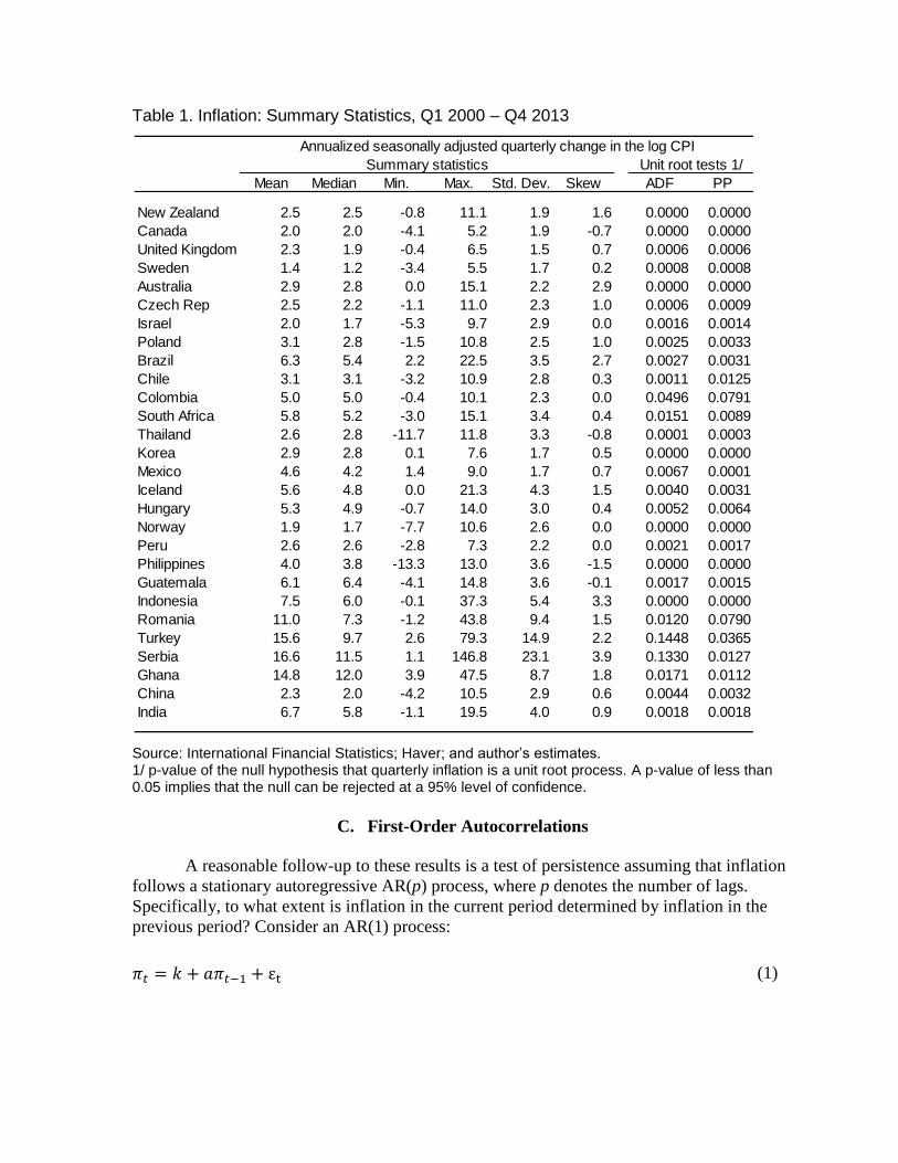
Table 1. Inflation: Summary Statistics, Q1 2000 – Q4 2013
Source: International Financial Statistics; Haver; and author’s estimates. 1/ p-value of the null hypothesis that quarterly inflation is a unit root process. A p-value of less than 0.05 implies that the null can be rejected at a 95% level of confidence.
C. First-Order Autocorrelations
A reasonable follow-up to these results is a test of persistence assuming that inflation
follows a stationary autoregressive AR(p) process, where p denotes the number of lags.
Specifically, to what extent is inflation in the current period determined by inflation in the
previous period? Consider an AR(1) process:
(1)
Annualized seasonally adjusted quarterly change in the log CPI
Summary statistics Unit root tests 1/
Mean Median Min. Max. Std. Dev. Skew ADF PP
New Zealand 2.5 2.5 -0.8 11.1 1.9 1.6 0.0000 0.0000
Canada 2.0 2.0 -4.1 5.2 1.9 -0.7 0.0000 0.0000
United Kingdom 2.3 1.9 -0.4 6.5 1.5 0.7 0.0006 0.0006
Sweden 1.4 1.2 -3.4 5.5 1.7 0.2 0.0008 0.0008
Australia 2.9 2.8 0.0 15.1 2.2 2.9 0.0000 0.0000
Czech Rep 2.5 2.2 -1.1 11.0 2.3 1.0 0.0006 0.0009
Israel 2.0 1.7 -5.3 9.7 2.9 0.0 0.0016 0.0014
Poland 3.1 2.8 -1.5 10.8 2.5 1.0 0.0025 0.0033
Brazil 6.3 5.4 2.2 22.5 3.5 2.7 0.0027 0.0031
Chile 3.1 3.1 -3.2 10.9 2.8 0.3 0.0011 0.0125
Colombia 5.0 5.0 -0.4 10.1 2.3 0.0 0.0496 0.0791
South Africa 5.8 5.2 -3.0 15.1 3.4 0.4 0.0151 0.0089
Thailand 2.6 2.8 -11.7 11.8 3.3 -0.8 0.0001 0.0003
Korea 2.9 2.8 0.1 7.6 1.7 0.5 0.0000 0.0000
Mexico 4.6 4.2 1.4 9.0 1.7 0.7 0.0067 0.0001
Iceland 5.6 4.8 0.0 21.3 4.3 1.5 0.0040 0.0031
Hungary 5.3 4.9 -0.7 14.0 3.0 0.4 0.0052 0.0064
Norway 1.9 1.7 -7.7 10.6 2.6 0.0 0.0000 0.0000
Peru 2.6 2.6 -2.8 7.3 2.2 0.0 0.0021 0.0017
Philippines 4.0 3.8 -13.3 13.0 3.6 -1.5 0.0000 0.0000
Guatemala 6.1 6.4 -4.1 14.8 3.6 -0.1 0.0017 0.0015
Indonesia 7.5 6.0 -0.1 37.3 5.4 3.3 0.0000 0.0000
Romania 11.0 7.3 -1.2 43.8 9.4 1.5 0.0120 0.0790
Turkey 15.6 9.7 2.6 79.3 14.9 2.2 0.1448 0.0365
Serbia 16.6 11.5 1.1 146.8 23.1 3.9 0.1330 0.0127
Ghana 14.8 12.0 3.9 47.5 8.7 1.8 0.0171 0.0112
China 2.3 2.0 -4.2 10.5 2.9 0.6 0.0044 0.0032
India 6.7 5.8 -1.1 19.5 4.0 0.9 0.0018 0.0018

In (1), the measure of persistence is the parameter a, where t is quarterly inflation in period
t, k is a constant, and ε is an iid shock to inflation. Expressing (1) in moving average form, a
can be regarded as the persistence of all previous inflation shocks ε.
(2)
I estimate a in (1) with OLS and without correction for bias since there is no evidence
that quarterly inflation for the countries in this sample either exhibits a time trend or is a
“near-unit root” process in the sense of Andrews and Chen (1994). An interesting way to
understand the parameter a is by calculating half-lives. This is the estimated time taken for
half of a shock to the quarterly inflation rate to fade. Based on an estimate of the regression
(1) over 2000 Q1 to 2013 Q2, Figure 1 presents estimated half-lives and 95 percent
confidence intervals (with the lower interval bounded at zero). Half lives for shocks to
headline inflation range from less than half of one quarter (Canada and New Zealand) to over
four quarters (Romania). Latin American countries, including Brazil, are mainly in the upper
end of the range but are broadly comparable with their IT peer group.
Figure1. Inflation Shock Half-Lives, Q1 2000 – Q4 2013
Source: Author’s estimates.
I find that generalizing the AR(1) model to incorporate more lags, as done for
example by Benati (2008) and Capistrán and Ramos-Francia (2009), is unnecessary for most
countries. Partial autocorrelations estimate that the impact of changes in inflation two or
more quarters earlier are typically insignificant for the current quarter’s inflation (not
shown); specifically, lags of p>1 were statistically significant for only one country for
headline inflation out of a total sample size of 33 countries.
0.0
0.5
1.0
1.5
2.0
2.5
3.0
3.5
4.0
4.5
5.0
Ro
man
ia
Turk
ey
Co
lom
bia
Russia
Ch
ile
Serb
ia
So
uth
Afr
ica
Gh
an
a
Po
lan
d
Ch
ina
Hun
gary
Icela
nd
Bra
zil
Peru
Isra
el
Guate
mala
Ind
ia
Cze
ch
Rep
Sw
ed
en
Un
ited
…
Sw
itze
rlan
d
Mexic
o
Th
ailand
Euro
Are
a
Jap
an
Ph
ilip
pin
es
Un
ited
Sta
tes
Ind
onesi
a
Ko
rea
New
Zeala
nd
Can
ad
a
Half-life Upper 95 percent confidence interval
Headline Inflation Shock Half-Lives, 2000-2012
(estimated from AR(1) equations)
D. Rolling Regressions
A more serious problem for an assessment of persistence than the number of lags is its time
variation. In fact, estimates of persistence can change dramatically based on the sample
period used, particularly in Latin America and Brazil. But the shift to lower persistence is
unlikely to be discrete and may happen only gradually, as credibility in the new policy
regime is accumulated over time.
To account for time variation, I estimate half-lives using the parameter a from (1)
with shorter rolling samples. Figures 2a and 2b show estimated half-lives from regressions
estimated over overlapping rolling 8 year samples of quarterly data. I use this window size as
it balances the objectives of adequately assessing time-variation with estimation using
sufficiently large sample periods. Specifically, the sample of the first estimation is Q1 1995
through Q4 2002. The second sample then starts and finishes one quarter later, from Q2 1995
through Q1 2003 and so on. The dates on the horizontal axis of the charts in Figure 2 refer to
the end date of the estimations. When a ≤ 0, the half-life is not defined and is represented by
breaks in the time series. In some cases, the half-life for large parts of the sample is not
defined but these data are shown for completeness (e.g., Norway). When it is not possible to
reject the null hypothesis that the parameter a (and the half-life) is zero, the lower 95 percent
confidence interval for the half-life is not defined and only the upper interval is shown.
The benchmark cases remain Canada and New Zealand with rolling half-lives that are
both low and statistically insignificant. More broadly, experiences vary by country but for
Latin America, there is no clear evidence (with one exception) that persistence is declining
firmly towards the low levels of Canada or New Zealand. In some cases, persistence fell
during the early years of IT (e.g., Colombia and Peru). But for most countries in the region
persistence since 2008 has remained broadly constant and statistically significant (Chile) or
increased (Colombia, Guatemala, and Peru). The one exception is Mexico, where persistence
is now statistically insignificant following the large sustained decline that followed the
introduction of IT in 2001.
In Brazil, inflation persistence appears to have been rising again following a
substantial fall in the half-life from almost 2 quarters in 2010. In fact, this apparent step-
decline in persistence is mainly due to the 2002-03 period falling out of the 8-year sample
window. Excluding this effect (for example by selecting samples that start in 2004),
persistence has been more stable. At the same time, persistence has increased since 2009. I
will show that this result, in which current assessments may be strongly influenced by
historical outliers and less by more recent development, also highlights an important
drawback of the backward-looking autoregressive approach.

Figure 2a. Inflation Shock Half-Lives, 2002-Q1 to 2013-Q4
Source: Author’s estimates
0
1
2
3
4
5
02 04 06 08 10 12
New Zealand
0
1
2
3
4
5
02 04 06 08 10 12
Canada
0
1
2
3
4
5
02 04 06 08 10 12
U.K.
0
1
2
3
4
5
02 04 06 08 10 12
Sw eden
0
1
2
3
4
5
02 04 06 08 10 12
Australia
0
1
2
3
4
5
02 04 06 08 10 12
Czech Rep
0
1
2
3
4
5
02 04 06 08 10 12
Israel
0
1
2
3
4
5
02 04 06 08 10 12
Poland
0
1
2
3
4
5
02 04 06 08 10 12
Brazil
0
1
2
3
4
5
02 04 06 08 10 12
Chile
0
1
2
3
4
5
02 04 06 08 10 12
Colombia
0
1
2
3
4
5
02 04 06 08 10 12
South Africa
0
1
2
3
4
5
02 04 06 08 10 12
Thailand
0
1
2
3
4
5
02 04 06 08 10 12
Korea
0
1
2
3
4
5
02 04 06 08 10 12
Mexico
0
1
2
3
4
5
02 04 06 08 10 12
Iceland
0
1
2
3
4
5
02 04 06 08 10 12
Hungary
0
1
2
3
4
5
02 04 06 08 10 12
Norw ay
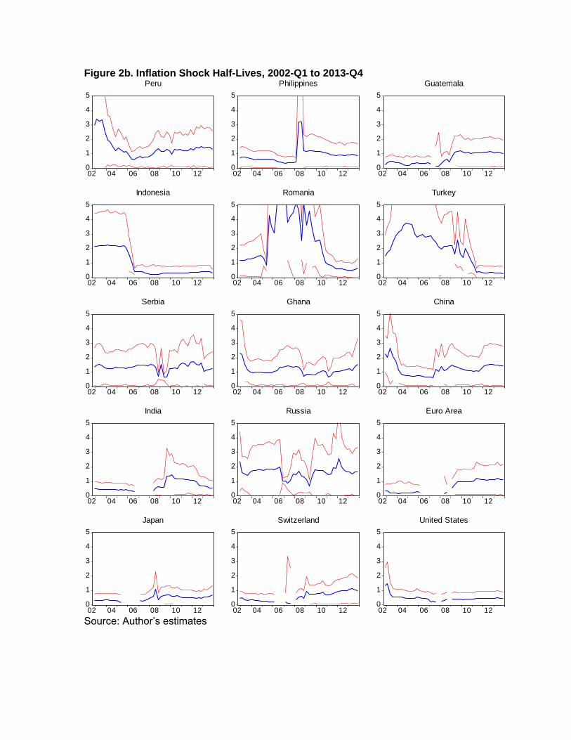
Figure 2b. Inflation Shock Half-Lives, 2002-Q1 to 2013-Q4
Source: Author’s estimates
0
1
2
3
4
5
02 04 06 08 10 12
Peru
0
1
2
3
4
5
02 04 06 08 10 12
Philippines
0
1
2
3
4
5
02 04 06 08 10 12
Guatemala
0
1
2
3
4
5
02 04 06 08 10 12
Indonesia
0
1
2
3
4
5
02 04 06 08 10 12
Romania
0
1
2
3
4
5
02 04 06 08 10 12
Turkey
0
1
2
3
4
5
02 04 06 08 10 12
Serbia
0
1
2
3
4
5
02 04 06 08 10 12
Ghana
0
1
2
3
4
5
02 04 06 08 10 12
China
0
1
2
3
4
5
02 04 06 08 10 12
India
0
1
2
3
4
5
02 04 06 08 10 12
Russia
0
1
2
3
4
5
02 04 06 08 10 12
Euro Area
0
1
2
3
4
5
02 04 06 08 10 12
Japan
0
1
2
3
4
5
02 04 06 08 10 12
Switzerland
0
1
2
3
4
5
02 04 06 08 10 12
United States
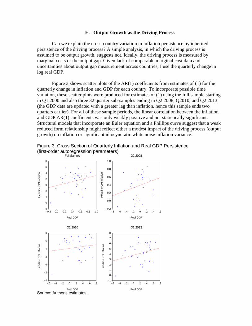
E. Output Growth as the Driving Process
Can we explain the cross-country variation in inflation persistence by inherited
persistence of the driving process? A simple analysis, in which the driving process is
assumed to be output growth, suggests not. Ideally, the driving process is measured by
marginal costs or the output gap. Given lack of comparable marginal cost data and
uncertainties about output gap measurement across countries, I use the quarterly change in
log real GDP.
Figure 3 shows scatter plots of the AR(1) coefficients from estimates of (1) for the
quarterly change in inflation and GDP for each country. To incorporate possible time
variation, these scatter plots were produced for estimates of (1) using the full sample starting
in Q1 2000 and also three 32 quarter sub-samples ending in Q2 2008, Q2010, and Q2 2013
(the GDP data are updated with a greater lag than inflation, hence this sample ends two
quarters earlier). For all of these sample periods, the linear correlation between the inflation
and GDP AR(1) coefficients was only weakly positive and not statistically significant.
Structural models that incorporate an Euler equation and a Phillips curve suggest that a weak
reduced form relationship might reflect either a modest impact of the driving process (output
growth) on inflation or significant idiosyncratic white noise inflation variance.
Figure 3. Cross Section of Quarterly Inflation and Real GDP Persistence (first-order autoregression parameters)
Source: Author’s estimates.
-.8
-.6
-.4
-.2
.0
.2
.4
.6
.8
-0.2 0.0 0.2 0.4 0.6 0.8 1.0
Real GDP
He
adlin
e C
PI In
fla
tion
Full Sample
-0.2
0.0
0.2
0.4
0.6
0.8
1.0
-.8 -.6 -.4 -.2 .0 .2 .4 .6
Real GDP
He
adlin
e C
PI In
fla
tion
Q2 2008
-.4
-.2
.0
.2
.4
.6
.8
-.6 -.4 -.2 .0 .2 .4 .6 .8
Real GDP
He
adlin
e C
PI In
flation
Q2 2010
-.1
.0
.1
.2
.3
.4
.5
.6
.7
.8
-.6 -.4 -.2 .0 .2 .4 .6 .8
Real GDP
He
adlin
e C
PI In
flation
Q2 2013
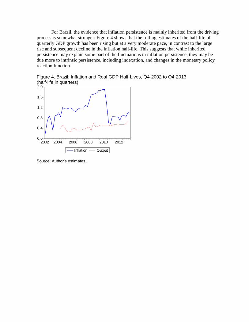
For Brazil, the evidence that inflation persistence is mainly inherited from the driving
process is somewhat stronger. Figure 4 shows that the rolling estimates of the half-life of
quarterly GDP growth has been rising but at a very moderate pace, in contrast to the large
rise and subsequent decline in the inflation half-life. This suggests that while inherited
persistence may explain some part of the fluctuations in inflation persistence, they may be
due more to intrinsic persistence, including indexation, and changes in the monetary policy
reaction function.
Figure 4. Brazil: Inflation and Real GDP Half-Lives, Q4-2002 to Q4-2013 (half-life in quarters)
Source: Author’s estimates.
0.0
0.4
0.8
1.2
1.6
2.0
2002 2004 2006 2008 2010 2012
Inflation Output
III. FORWARD LOOKING PERSISTENCE
Central banks require a good understanding of inflation persistence now and in the future
when calibrating policies. Estimates based on historical data are an obvious starting point,
but this approach can be slow to pick up changes in persistence as they happen. This is
because, by construction, the estimates are telling us what has occurred in the past. Reducing
sample size to increase the weight on more recent observations, such as the rolling
estimations in section II, is one answer to obtain more time-sensitive estimates but this can
leave the results dependent on a small number of outliers.
An alternative approach is to use expectations of inflation. If expectations are “good”
forecasters of future inflation, then persistence may be reliably measured by assessing the
impact of changes in actual inflation on these expectations. The idea is to identify whether,
and by how much, a shock to inflation today leads to a rise in expected inflation for some
future period. If surveyed expectations then influence the behavior of price-setters in the
economy, then this would provide a more timely indication of how long inflation shocks will
persist. Before moving to the first step in this approach—testing the forecasting properties of
inflation expectations—I will describe the data to be used in this section.
A. Data
Inflation is measured each month by the annual change in the headline consumer price index
for each country over a sample period of January 2000 through January 2014. Inflation
expectations are the predictions for this annual rate of inflation 12 months ahead.
Expectations are measured by the responses from surveys conducted by central banks,
statistical agencies, and in some cases private research firms in IT countries. I include all
countries for which a relatively long time series of inflation expectations exists. The actual
timing of these surveys each month can vary but where there is an option to choose (e.g.,
from the weekly Focus survey for Brazil) I select the latest available data point to maximize
the probability that the survey reflects all relevant information.
A statistical summary of the data is provided in Table 2 and unit root tests (indicating
that almost all series are stationary) are presented in Table 3. For those countries for which
the variables are non-stationary, there was strong evidence that the inflation and inflation
expectations are cointegrated.

Table 2. Annual Inflation and 12-Month Inflation Expectations: Summary Statistics (percent unless specified otherwise)
Source: Author’s calculations.
Table 3. Annual Inflation and 12-Month Inflation Expectations: Unit Roots and Cointegration (p-values of the null hypotheses of a unit root or no cointegration)
Source: Author’s calculations.
Headline CPI Inflation 12-Month Expected Inflation
Number of Standard Standard
observations Mean Min. Max. deviation Mean Min. Max. deviation
Brazil 147 6.54 2.96 17.24 2.93 5.36 3.43 12.52 1.45
Chile 104 3.46 -2.29 9.85 2.57 3.21 2.00 6.00 0.67
Colombia 124 4.32 1.75 7.94 1.68 4.21 2.87 6.10 0.87
Mexico 170 4.88 2.91 12.32 1.71 4.53 3.42 11.14 1.52
Peru 143 2.69 -1.08 6.75 1.59 2.60 1.63 4.71 0.58
Czech Republic 170 2.56 -0.42 7.55 1.71 2.92 1.40 5.00 0.83
Israel 170 2.10 -2.74 6.94 2.02 2.29 0.30 4.10 0.64
Poland 170 3.42 0.16 11.64 2.46 3.50 0.20 13.50 2.76
Turkey 109 8.30 3.99 12.06 1.81 6.83 5.42 8.99 0.71
Korea 170 2.95 0.85 5.98 1.04 3.55 2.80 4.60 0.56
Canada 170 2.02 -0.95 4.68 0.97 1.94 0.58 2.70 0.39
Unit root tests . Cointegration tests 1/
Engle-Granger Philips-Perron
Headline Expected Headline Expected Johansen Engle-Granger
Inflation Inflation Inflation Inflation Test Test
Brazil 0.045 0.012 0.200 0.071 … …
Chile 0.023 0.005 0.247 0.098 … …
Colombia 0.343 0.449 0.422 0.451 0.00 0.31
Mexico 0.002 0.000 0.000 0.000 … …
Peru 0.036 0.152 0.034 0.044 … …
Czech Republic 0.289 0.254 0.121 0.233 0.01 0.16
Israel 0.050 0.002 0.046 0.000 … …
Poland 0.065 0.223 0.129 0.172 0.00 0.17
Turkey 0.082 0.000 0.082 0.006 … …
Korea 0.106 0.349 0.051 0.180 0.05 0.47
Canada 0.014 0.000 0.008 0.014 … …

B. Inflation Expectations as Forecasters
As a first step, I assess whether inflation expectations provide unbiased and competitive
forecasts of actual inflation. To test in-sample bias, I estimate the following regression for
each country where both actual and expected inflation are stationary:
(3)
The endogenous variable is the actual change in the annual inflation rate over a 12
month period. The exogenous variable is the change in the inflation rate over this same
period predicted 12 months previously by the survey. The first two columns of Table 4
present the estimates of the coefficients α and β from (3) over the largest sample available for
each country over a maximum sample period of Jan-2000 through Jan-2014. The third
column in Table 4 presents the results from a test of the null hypothesis that inflation
expectations are in-sample unbiased. This is a joint test of the restrictions in (1) that α=0 and
β=1. All of the indicators of significance and hypothesis tests in Table 4 use Newey-West
standard errors with a bandwidth appropriate to accommodate the serial correlation
introduced by using overlapping observations. The results show that this null hypothesis can
be rejected at the 5 percent level in 5 out of 11 cases. In Brazil, bias is due to persistent
underestimation (a positive and significant α coefficient). In most other cases, expectations
do not make persistent directional errors but they do tend to underestimate the volatility of
inflation (a β coefficient greater than one).
Table 4. Inflation Expectations: In-Sample Tests of Bias, Jan-2000 to Sep-2013
Source: Author’s estimates.
In-sample tests of efficiency and bias can tell us whether expectations may be useful
for forecasting, but they do not evaluate their forecast accuracy (and hence their use as
indicators of future inflation persistence). As Granger and Newbold (1977) argue, the
distributional properties of forecasting variables and actual values are almost always
Constant Coefficient Wald
α β test
Brazil 1.14 ** 1.00 *** 0.0604
Chile 0.35 1.32 *** 0.4690
Colombia -0.18 0.92 ** 0.7990
Mexico -0.06 1.08 *** 0.8412
Peru 0.31 1.58 *** 0.0369
Czech Republic -0.65 * 1.38 *** 0.0003
Israel -0.17 1.18 *** 0.7600
Poland -0.58 -0.87 * 0.0001
Turkey 0.81 1.71 *** 0.0000
Korea -0.59 * 0.93 *** 0.1313
Canada 0.13 1.68 *** 0.0019

different; as a result, a direct comparison of the two is of limited use. The real test of the
utility of expectations is their out-of-sample forecasting properties. Figure 5 compares the
performance of survey expectations against a random walk, core inflation, and the inflation
target. The figures represent the difference between the root mean squared error (RMSE) for
expected inflation and each of the naive forecasts. In most cases, RMSEs for inflation
expectations are substantially lower (indicated by negative values in Figure 5). Forecasting
performance was compared over the whole sample and also for a sample starting in January
2004 to remove the effect of very high inflation volatility from the results for Brazil.
Figure 5. Inflation Expectations Forecast performance Root Mean Squared Error (compared to naive forecasts, percentage points)
Source: Author’s estimates.
From this I conclude that while inflation expectations exhibit some shortcomings as a
forecasting tool, they are still hard to beat out-of-sample, at least using naive methods
including core inflation.
C. Forward-Looking Persistence Using Expectations
On this basis, I use expectations to provide a more forward-looking assessment of inflation
persistence. Specifically, I assume that inflation exhibits more (less) persistence the greater
(lesser) is the effect of a change in actual inflation on expected inflation at some future date.
The specification for the estimations is:
-1.5 -0.5 0.5 1.5
Brazil
Chile
Colombia
Mexico
Peru
Czech Republic
Israel
Poland
Turkey
Korea
Canada
Random walk
Core inflation
Inflation target
Sample: January 2000 - January 2014
-1.5 -0.5 0.5 1.5
Brazil
Chile
Colombia
Mexico
Peru
Czech Republic
Israel
Poland
Turkey
Korea
Canada
Random walk
Core inflation
Inflation target
Sample: January 2004 - January 2014

Where:
(4)
The endogenous variable is the change in expected annual inflation at a rolling 12-
month horizon in the current month compared to the previous month. The first exogenous
variable is the change in the actual annual inflation rate lagged by one month. I have lagged
this variable for two reasons: it ensures that expectations have the time necessary to
incorporate fully any relevant information from actual inflation which is often reported with
a short lag; and it avoids issues of endogeneity as changes in expectations can affect price-
setting behavior. The coefficient γ1 measures persistence. The second exogenous variable is
change in expected annual inflation lagged by one month to capture slow-moving changes in
expectations, including due to herd behavior among analysts.
I estimate an alternative specification to admit the possibility that inflation shocks of
different signs exhibit varying persistence. For example, a rise in actual inflation may have a
larger effect than a fall on expected inflation. This asymmetry might result from the market’s
perception that monetary and other policies may respond differently to falling inflation than
to rising inflation based on an understanding of the policymaker’s loss function. This
specification is given by
(5)
This specification is identical to (4) with the following difference: the dummy variables d1
and d2 take on the values 1 and 0 when the lagged change in actual inflation is positive and
negative, respectively. I then interpret γ1 and γ2 as measures of upward and downward
inflation persistence, respectively.
I estimate equations (4) and (5) using OLS and Newey-West standard errors for all 11
countries using all of the available data. The first column of Table 6 shows the estimate of
forward-looking persistence using the symmetric specification—i.e., coefficient γ1 from (4).
The second and third columns show the estimates of persistence from the asymmetric
specification—i.e., coefficients γ1 and γ2 from (5).
The results show that forward-looking persistence is still quite high and statistically
significant, particularly among emerging market countries. For example, on average over the
sample period in Poland over ⅓ of any given percentage point change in actual inflation is
passed on to expected inflation 12 months ahead. Persistence is lower among the advanced
economies. A second result is that in Brazil and other Latin American countries, upward

persistence is larger and more often statistically significant that downward persistence. In
particular, a rise in inflation passes through to expectations. In contrast the pass through from
a decline in inflation to expectations is either smaller or insignificant. This asymmetry is
particularly striking in Brazil.
Table 6. Effects of Actual Inflation on Expected Inflation, Jan-2000 to Jan-2014
Source: Authors’ estimates.
For Brazil, evidence of asymmetry is important for understanding how inflation
expectations are formed and actual inflation persists. One interpretation is that the historical
legacy of high and persistent inflation appears to have endured through the first 10-15 years
of inflation targeting. Institutionalized indexation and other remnants of a high inflation past
may take time to dismantle. This underscores the difficult task policymakers have had in
building inflation credibility but, as credibility is gained, holds out the reward of less
persistent inflation in the future. A second possible interpretation is that markets correctly
perceive some asymmetry in policymakers’ reaction function, with more willingness to
tackle falling inflation (and associated declines in output growth) and greater tolerance of
rising inflation (and higher output).
A simple reduced form model cannot provide conclusive answers as to which
interpretation is correct but an enhanced empirical approach can shed some light on the
mystery. Consider estimates based on rolling samples. If forward-looking persistence
(particularly upward persistence) is declining over time, then this would be more consistent
with the first, more benign, interpretation of the results in Table 6. In contrast, if upward
persistence were stable or even rising, then this would be more consistent with the second
interpretation related to asymmetries of policy reaction functions.
Figure 6 presents estimates of upward inflation persistence—coefficient γ1 from (5)—
for rolling 60-month samples using all available data for each country. The estimates shown
for some countries include those from windows with less than 60 observations which explain
Coefficient on
Lagged Coefficients on Lagged Inflation Sample
Inflation Change Increases Decreases size
Brazil 0.11 * 0.18 * 0.06 146
Chile 0.14 *** 0.16 *** 0.12 ** 103
Colombia 0.19 *** 0.24 *** 0.16 *** 123
Mexico 0.09 *** 0.13 ** 0.05 168
Peru 0.16 *** 0.17 *** 0.16 *** 142
Czech Republic 0.11 *** 0.11 * 0.10 ** 168
Israel 0.02 0.02 0.03 168
Poland 0.36 *** 0.35 *** 0.36 *** 168
Turkey 0.13 *** 0.14 *** 0.12 *** 109
Korea 0.12 *** 0.17 *** 0.09 ** 143
Canada 0.05 ** 0.05 * 0.04 168
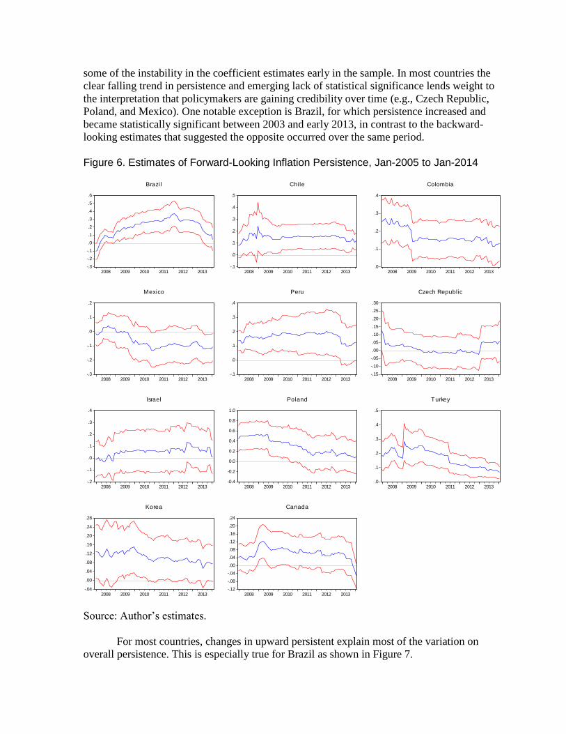
some of the instability in the coefficient estimates early in the sample. In most countries the
clear falling trend in persistence and emerging lack of statistical significance lends weight to
the interpretation that policymakers are gaining credibility over time (e.g., Czech Republic,
Poland, and Mexico). One notable exception is Brazil, for which persistence increased and
became statistically significant between 2003 and early 2013, in contrast to the backward-
looking estimates that suggested the opposite occurred over the same period.
Figure 6. Estimates of Forward-Looking Inflation Persistence, Jan-2005 to Jan-2014
Source: Author’s estimates.
For most countries, changes in upward persistent explain most of the variation on
overall persistence. This is especially true for Brazil as shown in Figure 7.
-.3
-.2
-.1
.0
.1
.2
.3
.4
.5
.6
2008 2009 2010 2011 2012 2013
Brazil
-.1
.0
.1
.2
.3
.4
.5
2008 2009 2010 2011 2012 2013
Chile
.0
.1
.2
.3
.4
2008 2009 2010 2011 2012 2013
Colombia
-.3
-.2
-.1
.0
.1
.2
2008 2009 2010 2011 2012 2013
Mexico
-.1
.0
.1
.2
.3
.4
2008 2009 2010 2011 2012 2013
Peru
-.15
-.10
-.05
.00
.05
.10
.15
.20
.25
.30
2008 2009 2010 2011 2012 2013
Czech Republic
-.2
-.1
.0
.1
.2
.3
.4
2008 2009 2010 2011 2012 2013
Israel
-0.4
-0.2
0.0
0.2
0.4
0.6
0.8
1.0
2008 2009 2010 2011 2012 2013
Poland
.0
.1
.2
.3
.4
.5
2008 2009 2010 2011 2012 2013
Turkey
-.04
.00
.04
.08
.12
.16
.20
.24
.28
2008 2009 2010 2011 2012 2013
Korea
-.12
-.08
-.04
.00
.04
.08
.12
.16
.20
.24
2008 2009 2010 2011 2012 2013
Canada
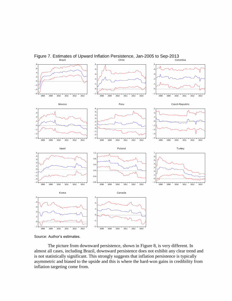
Figure 7. Estimates of Upward Inflation Persistence, Jan-2005 to Sep-2013
Source: Author’s estimates.
The picture from downward persistence, shown in Figure 8, is very different. In
almost all cases, including Brazil, downward persistence does not exhibit any clear trend and
is not statistically significant. This strongly suggests that inflation persistence is typically
asymmetric and biased to the upside and this is where the hard-won gains in credibility from
inflation targeting come from.
-.6
-.4
-.2
.0
.2
.4
.6
.8
2008 2009 2010 2011 2012 2013
Brazil
-.1
.0
.1
.2
.3
.4
.5
2008 2009 2010 2011 2012 2013
Chile
-.1
.0
.1
.2
.3
.4
.5
2008 2009 2010 2011 2012 2013
Colombia
-.3
-.2
-.1
.0
.1
.2
.3
.4
2008 2009 2010 2011 2012 2013
Mexico
-.3
-.2
-.1
.0
.1
.2
.3
.4
.5
.6
2008 2009 2010 2011 2012 2013
Peru
-.4
-.3
-.2
-.1
.0
.1
.2
.3
2008 2009 2010 2011 2012 2013
Czech Republic
-.4
-.3
-.2
-.1
.0
.1
.2
.3
.4
.5
2008 2009 2010 2011 2012 2013
Israel
-0.8
-0.4
0.0
0.4
0.8
1.2
2008 2009 2010 2011 2012 2013
Poland
-.1
.0
.1
.2
.3
.4
.5
.6
.7
2008 2009 2010 2011 2012 2013
Turkey
-.1
.0
.1
.2
.3
.4
.5
2008 2009 2010 2011 2012 2013
Korea
-.2
-.1
.0
.1
.2
.3
2008 2009 2010 2011 2012 2013
Canada

Figure 8. Estimates of Forward-Looking Downward Inflation Persistence
Source: Author’s estimates.
IV. CONCLUSION
Assessing inflation persistence using historical data may provide misleading conclusions.
Brazil’s inflation persistence, as measured using historical data and reduced-form
autoregression models, appeared to decline suddenly in 2010 and sit within the range found
among its inflation targeting peers. This suggests that inflation targeting has helped the
country overcome is history of indexation by building credibility in the notion that inflation
will remain anchored at the target and that temporary inflation shocks will quickly dissipate.
But looking at historical data is, of course by definition, backward looking and may not
-.4
-.3
-.2
-.1
.0
.1
.2
.3
.4
.5
2008 2009 2010 2011 2012 2013
Brazil
-.6
-.4
-.2
.0
.2
.4
.6
.8
2008 2009 2010 2011 2012 2013
Chile
-.1
.0
.1
.2
.3
.4
.5
2008 2009 2010 2011 2012 2013
Colombia
-.5
-.4
-.3
-.2
-.1
.0
.1
.2
2008 2009 2010 2011 2012 2013
Mexico
-.1
.0
.1
.2
.3
.4
.5
2008 2009 2010 2011 2012 2013
Peru
-.2
-.1
.0
.1
.2
.3
.4
.5
2008 2009 2010 2011 2012 2013
Czech Republic
-.4
-.3
-.2
-.1
.0
.1
.2
.3
.4
.5
2008 2009 2010 2011 2012 2013
Israel
-0.6
-0.4
-0.2
0.0
0.2
0.4
0.6
0.8
1.0
2008 2009 2010 2011 2012 2013
Poland
.0
.1
.2
.3
.4
.5
2008 2009 2010 2011 2012 2013
Turkey
-.2
-.1
.0
.1
.2
.3
2008 2009 2010 2011 2012 2013
Korea
-.2
-.1
.0
.1
.2
.3
2008 2009 2010 2011 2012 2013
Canada

reflect important changes at the margin. Indeed, there has been some pick-up in Brazil’s
inflation persistence, notably upward persistence, when it is measured by the impact of
changes on actual inflation on forward-looking expectations. The utility of this method relies
on an assumption that inflation expectations provide reasonably effective out-of-sample
forecasts and, for most countries, this is true. By using expectations, I can provide a more up-
to-date estimate of inflation since the sample period effectively extends into the future.
Rising upward inflation persistence in Brazil between 2002 and early 2013 could
signal that market participants believed that policymakers had become less responsive to
rising, rather than falling, inflation. For example, if the economy experienced a positive
inflation shock resulting from a transitory supply disturbance, there could be a perception
that monetary policy would not respond as forcefully to minimize the second-round effects
on underlying inflation. This would clearly be evident in a large effect of current inflation
surprises on estimates of future inflation. An alternative explanation could be that intrinsic
persistence is rising due, for example, to more prevalent indexation. The reduced-form
empirical strategy I use in this paper cannot conclusively identify which is the correct
explanation.
What I can conclude is that this increase in upward inflation persistence in Brazil was
in contrast to many other IT countries, including other emerging markets. In many of these
other countries, persistence had tended to gradually decline, consistent with a gradual buildup
of policy credibility and increasingly well-anchored inflation expectations. Although upward
persistence showed some early signs of falling during the central bank’s rate hiking cycle in
2013, this trend has paused and Brazil’s statistically significant inflation persistence
continues to stand in sharp contrast to the low persistence benchmark economies such as
Canada and New Zealand.

REFERENCES
Andrews, Donald W. K, and Hong-Yuan Chen, 1994, “Approximately Median-Unbiased
Estimation of Autoregressive Models,” Journal of Business & Economic Statistics, Vol. 12,
Issue 2, pp. 187-204.
Benati, Luca, 2008, “Investigating Inflation Persistence Across Monetary Regimes,”
Quarterly Journal of Economics, pp. 1005-1060.
Capistrán, Carlos and Manuel Ramos-Francia, 2009, “Inflation Dynamics In Latin America,”
Contemporary Economic Policy, vol. 27(3), pp. 349-362.
Fuhrer, Jeffrey C., 2010, “Inflation Persistence,” Chapter 9 in Handbook of Monetary
Economics, Ed. Benjamin M. Friedman and Michael Woodford, Elsevier, pp 423-486.
Granger, C. W. J., and Paul Newbold, 1977, Forecasting Economic Time Series, Academic Press,
New York.
Gürkaynak, Refet S, Andrew T. Levin, and Eric T. Swanson, 2010, “Does Inflation Targeting
Anchor Long-Run Inflation Expectations? Evidence from Long-Term Bond Yields in the
U.S., U.K., and Sweden,” Journal of the European Economic Association, Volume 8, Issue
6, pp 1208–1242.
Lucas, Robert, 1976, “Econometric Policy Evaluation: A Critique,” in The Philips Curve and
Labor Markets, Carnegie-Rochester Series on Public Policy, Vol. 1, pp. 19-46.
Mishkin, Frederic S. and Klaus Schmidt-Hebbel, 2007, “Does Inflation Targeting Make a
Difference?” in Monetary Policy under Inflation Targeting, Edited by Frederic S. Miskin,
Klaus Schmidt-Hebbel, and Norman Loayz, Edition 1, Volume 11, Chapter 9, Central Bank
of Chile.
Roger, Scott, 2010, “Inflation Targeting Turns 20,” Finance and Development, International
Monetary Fund, Washington D.C.