inferring temporal information from a snapshot of a ... · inferring temporal information from a...
TRANSCRIPT

Inferring Temporal Information from a Snapshot of aDynamic NetworkJithin K. Sreedharan1,+, Abram Magner1,+, Ananth Grama1, and Wojciech Szpankowski1,*
1Center for Science of Information, Dept. of Computer Science, Purdue University, USA*To whom correspondence should be addressed. E-mail: [email protected]+These authors contributed equally to this work
ABSTRACT
The problem of reverse-engineering the evolution of a dynamic network, known broadly as network archaeology, is oneof profound importance in diverse application domains. In analysis of infection spread, it reveals the spatial and temporalprocesses underlying infection. In analysis of biomolecular interaction networks (e.g., protein interaction networks), it revealsearly molecules that are known to be differentially implicated in diseases. In economic networks, it reveals flow of capital andassociated actors. Beyond these recognized applications, it provides analytical substrates for novel studies – for instance, onthe structural and functional evolution of the human brain connectome. In this paper, we model, formulate, and rigorouslyanalyze the problem of inferring the arrival order of nodes in a dynamic network from a single snapshot. We derive limits onsolutions to the problem, present methods that approach this limit, and demonstrate the methods on a range of applications,from inferring the evolution of the human brain connectome to conventional citation and social networks, where ground truth isknown.
IntroductionComplex systems are comprised of interacting entities; e.g., cellular processes are comprised of interacting genes, proteins,and other biomolecules; social systems, of individuals and organizations; and economic systems, of financial entities. Thesesystems are modeled as networks, with nodes representing entities and edges representing their interactions. Typical systemscontinually evolve to optimize various criteria, including function (e.g., flow of information in social networks, evolution ofbrain connectomes to specialize function), structure (e.g., evolution of social network structures to minimize sociological stresswhile maximizing information flow), and survivability (e.g., redundant pathways in genic interactions as evidenced by syntheticlethality screens). Recent results have also demonstrated advantages of dynamic networks in achieving quicker controllability1.Effective analysis of dynamic networks provides strong insights into the structure, function, and processes driving systemevolution.
The problem of inferring the evolution of a dynamic network is of considerable significance: in a network of financialtransactions, the arrival order of nodes tracks the flow of capital. In mapping spread of infectious diseases, node arrival orderallows one to identify early patients, yielding clues to genetic origin, evolution, and mechanisms of transmission. In networksof biochemical interactions (e.g., protein interaction networks2) one can identify early biomolecules that are known to bedifferentially implicated in diseases3. Recently, strategic seeding and spread of (mis)information in online social networks likeTwitter and Facebook has been hypothesized to create strong biases in opinions, even skewing electoral outcomes. Identifyingsources and mechanisms of information transfer enables us to quarantine sources in a timely manner and to control spread.
Our contributions. We model and formulate the problem of recovering the temporal order of nodes in general graph models.Focusing on preferential attachment graphs and on deriving fundamental limits on inference of temporal order, we show thatthere exists no estimator for recovering temporal arrival order with high probability, owing to inherent symmetries in networks.Motivated by this negative result, we relax the formulation to admit a partial order on nodes. In doing so, we allow the estimatorto make fewer vertex pair order inferences, in exchange for higher precision (e.g., by grouping nodes and finding the order onlybetween groups but not within groups). We refer to the fraction of all node pairs that is comparable by a partial order (in termsof the arrival order) as the partial order density. We cast the partial order inference problem as a rational linear integer program,which allows us to present detailed analytical results on the achievable limits in terms of the tradeoff between expected precisionand partial order density. To solve the optimization problem, we need to count the number of linear extensions of the partialorder, which is known to be #P-complete4. There exists a fully-polynomial-time approximation algorithm that approximatesthe optimal solution to arbitrarily small relative error. However, in view of its significant computational cost, we propose aMarkov chain Monte Carlo technique that achieves faster convergence in practice. We introduce and analyze, both theoretically
and empirically, efficient estimators: our first estimator is optimal in the sense that it yields perfect precision. It infers all vertexorder relations that hold with probability one. However, we find such relations to be asymptotically small compared to the totalnumber of correct pairs. This motivates our investigation of other algorithms (the PEELING and PEELING+ algorithms), whichsacrifice some precision in order to achieve higher density.
Experimental evaluation, on both synthetic and real-world datasets (network data of citations (ArXiv), collaborations(DBLP), hyperlinks (Wikipedia) and social connections (Facebook and SMS)), demonstrates the robustness of our methodsto variations from the preferential attachment model. We also present a novel application of our method to the analysis ofthe human brain connectome to identify regions of “early” and “late” development. Our results reveal novel insights into thestructural and functional evolution of the brain.
Prior works. The problem of inferring the sequence of node arrivals from a given network snapshot is highly complex, bothanalytically and methodologically, and has been little studied in prior literature. The works of Navlakha and Kingsford5 andYoung et al.6 are the ones closest to ours. Navlakha and Kingsford5 formulates the problem as a maximum a posterioriestimation problem and develops a greedy algorithm for different graph models. Such a study can be translated to our maximumlikelihood approach and we prove later that this leads to very large number of equiprobable solutions in the case of preferentialattachment graphs. Young et al.6 studies the phase transition of recoverability via numerical experiments in the case of anon-linear preferential attachment graph in the Bayesian framework, with respect to the non-linear exponent of degree. Sucha phase transition can be formally justified with the theoretical results in the Supplementary Material of this paper. Someprior results focus on variants of the problem of finding the oldest node in a graph7, 8. The results of Bubeck et al.7 are onlyapplicable to trees, thus severely limiting their application scope. Our proposed methods target general graphs and seek nodeorders beyond identifying the oldest node. Frieze et al.8 study the problem of identifying the oldest node in preferentialattachment graphs using a local exploratory process with the assumption that the time index of a node can be retrieved once it issampled. A related problem of detecting information sources in epidemic networks has been studied by Shah et al.9 and Zhu etal.10 for the Susceptible-Infected model. We first formulated the node arrival order inference problem and presented somepreliminary results in Ref 11.
Results
Let G be a graph of n vertices corresponding to a snapshot of a growing network, generated by a dynamic graph model. Withoutloss of generality, we count time in units of vertex additions. Since G has n vertices, we say that this is the snapshot at time n.We label vertices in their arrival order, [n] = 1, ...,n, where node j is the jth node to arrive. Note that these vertex labels arenot known to us. Instead, the vertices are randomly relabeled according to a permutation π drawn uniformly at random fromthe set of permutations on n letters Sn, and we are given the graph H := π(G). Our goal is to infer the arrival order of verticesin graph G from observed graph H, i.e., to find the inverse permutation π−1, which reveals the true arrival order. See Figure 1for an illustration of our approach and an application on inferring the evolutionary order of prominent human brain regions. Weprovide further analyses of this result later in the paper.
We consider a general scenario in which we do not restrict our analysis to inference of a total order. Rather, we consider anestimator φ that outputs partial orders on the set of vertices (see Figure 1A for an example). For a partial order σ , a relationu<σ v defined on vertices u and v means that vertex u’s label is less than that of vertex v in the partial order σ . We say that anordered pair of vertices (u,v) in π(G) satisfying u<σ v forms a correct pair if π−1(u)< π−1(v); i.e., vertex u precedes vertexv in the true arrival order. Given a partial order σ , we can always algorithmically find a total order consistent with σ (i.e., alinear extension of σ ).
We formally define measures for quantifying the performance of any estimator. For a partial order σ , let K(σ) denote thenumber of pairs u,v that are comparable under σ : i.e., K(σ) = |(u,v) : u<σ v|, where |K(σ)| ≤
(n2
).
Density: This is the number of comparable pairs in σ normalized by the total number of pairs, that is, δ (σ) = K(σ)
(n2). The density
of a partial order estimator φ is thus δ (φ) = minH∈Gn [δ (φ(H))], where Gn is the set of all graphs of size n.
Precision: This measures the expected fraction of correct pairs out of all pairs dictated by the partial order. That is,
θ(σ) = E[
1K(σ)
|u,v ∈ [n] : u<σ v,π−1(u)< π−1(v)|
].
For an estimator φ , we denote by θ(φ) the quantity E[θ(φ(π(G)))].Recall: This measures the expected fraction of correct pairs (out of the total number of pairs) output by an algorithm inferring a
2/31

GraphModel
Adversary
𝜋"# = 𝜎
Output 𝜎
𝐺' '(#)
Sequence ofgraphs
𝜋(𝐺))
𝐺) with permuted labels
Estimator
A
B
C
𝑡 = 1 𝑡 = 3 𝑡 = 5 𝑡 = 7 𝑡 = 9 𝑡 = 11 𝑡 = 16 𝑡 = 21
Figure 1. A. Block diagram of our formulation. B. A network of human brain formed from Human Connectome Project (HCP) data. Thisnetwork is shown as an example of π(GT ). Since the estimator should not dependent on the permutation, applying an unknown adversarypermutation on node labels is equivalent to making the graph unlabeled. C. Human brain evolution deduced by our method: Startingfrom network data in B, we apply our techniques and make an inference on how brain regions evolve in the left hemisphere of a human brain.The time instant t in the figure represents an instant of change in the evolution of brain regions. The data and code are available at12. SeeFigure 5 and the Methods for more details.
partial order σ , that is,
ρ(σ) = E
[1(n2
) |u,v ∈ [n] : u<σ v,π−1(u)< π−1(v)|
].
Figure 2A presents a sample graph, the permuted vertex labels, a candidate partial order, and measures of density, precision,and recall for the partial order.
We present our key results and illustrate them in the context of dynamic networks generated by Barabási-Albert preferentialattachment model. Many dynamic networks arising in a variety of applications are hypothesized to follow this model of“rich-gets-richer" mechanism13–19. We denote a dynamic graph generated by the preferential attachment model as PA (n,m)13,where n is the number of nodes and m is the number of connections a new node makes to existing nodes when it is addedto the network. At t = 1 a single vertex (labeled 1) is created with m self loops. To construct graph Gt at time 1 < t ≤ n,vertex t joins the network and makes m independent connections to the existing nodes in graph Gt−1 with probabilityPr[t connects to k|Gt−1] =
degt−1(k)2m(t−1) , where degt−1(k) is the degree of node k at time t−1. Let DAG(G) be the directed acyclic
version of G with the direction of edges marked in accordance with the graph evolution (leading from younger nodes to oldernodes). For π(G), edge directions are captured in its directed version π(DAG(G)). Note that DAG(G) and π(DAG(G)) havethe same structure. This is illustrated in Figure 2B.
If we restrict the estimator to output a total order, i.e., δ (σ) = 1, we show in SM Section 3 that no algorithm can solve theproblem with error probability asymptotically bounded away from 1. As a specific instance of a solution procedure, one mayalso frame the problem in terms of maximum likelihood estimation as follows:
CML(H) = argmaxσ∈Sn
Pr[π−1 = σ |π(G) = H].
We show that the set CML yields a large number of equiprobable solutions, |CML|= en logn−O(n log logn) with high probability,and therefore the maximum likelihood formulation is unsuitable. ( f (x) = O(g(x)) indicates that there exist δ > 0 and M > 0such that | f (x)| ≤M|g(x)| for |x−a|< δ .)
3/31

1
2
34
7
10
11
5 6
8
9
12
8
12
92
1
5
4
11 3
10
7
6
2 1
3 4
7
5
10116
89
12
12 8
9 2
1
11
543
107
6
A B
Figure 2. A. An example scenario. The estimator sees only π(G) and must infer π−1. E.g., it may output the order σ = 4≺ 1≺ 2 Therelation 4≺ 1 is correct, since π−1(4) = 3< π−1(1) = 4, but the relations 4≺ 2 and 1≺ 2 are incorrect, since π−1(4) = 3> π−1(2) = 2and π−1(1) = 4> π−1(2) = 2. The density is δ (σ) = 3/
(42)= 3/6 = 1/2, the precision is θ(σ) = 1/K(σ) = 1/3, and the recall is
ρ(σ) = θ(σ)δ (σ) = 1/6. B. The original graph (left) and the observed graph (right) for an instance of π: the same bin nodes in the DAGshave the same colors. Note that DAG(G) and π(DAG(G)) have exactly the same structure. The π(DAG(G)), generated by PEELING
algorithm recovers all the probability one order information of G.
Formulation and solution of the underlying optimization problem. In view of this negative result, we consider estimatorsoutputting a partial order on nodes. Here, an estimator may make fewer vertex pair order inferences, in exchange for higherprecision (e.g., by grouping nodes and inferring the order only across groups, but not within groups). We then seek an optimalestimator in the following sense: for an input parameter ε ∈ [0,1], we seek an estimator φ with density δ (φ)≥ ε and maximumpossible precision θ(φ). This yields an optimal curve θ∗(ε), that characterizes the tradeoff between precision and density. Wederive computable bounds on this curve and present efficient heuristic estimators that approach the bounds.
Given a graph H, define the function Jε(φ) as the fraction of correctly inferred vertex orderings from among all allowableorderings by a given partial order. That is,
Jε(φ) =E[|u,v ∈ [n] : u<φ(H) v,π−1(u)< π−1(v)|
∣∣∣π(G) = H]
K(φ(H)),
and the conditional expectation is with respect to the randomness in π and G. To exhibit an optimal estimator, it is sufficient tochoose, for each H, a value for φ(H) (i.e., a partial order) that maximizes the expression Jε(φ) subject to the density constraint,K(φ(H))≥ ε
(n2
). We can then write the precision of estimator φ as:
θ(φ) = ∑H
Pr[π(G) = H]Jε(φ).
To construct an optimal estimator, for each ordered pair (u,v) of vertices of H, we associate a binary variable xu,v, wheresetting xu,v = 1 indicates that u<φ(H) v. We can then rewrite Jε(φ) as:
Jε(φ) =∑1≤u<v≤n pu,v(H)xu,v
∑1≤u6=v≤n xu,v, (1)
where pu,v(H) = Pr[π−1(u)< π−1(v)|π(G) = H] is the probability that u arrived before v given the permuted graph H, withthe following constraints coming from the partial order and from our constraint on a given minimum density:1. Antisymmetry: xu,v + xv,u ≤ 1.
4/31
2. Transitivity: xu,w ≥ xu,v + xv,w−1 for all u,v,w ∈ [n].3. Minimum density: ∑1≤u6=v≤n xu,v ≥ ε
(n2
).
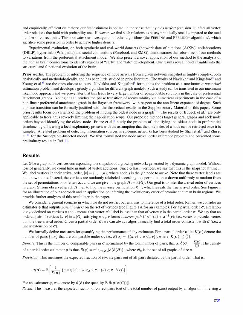
4. Domain restriction: xu,v ∈ 0,1 for all u,v ∈ [n].We efficiently upper bound the optimal precision for any given density constraint ε as follows: on a randomly generated inputgraph H = π(G), we recover its edge directions (i.e., π(DAG(G))) and use them to approximate the coefficients pu,v(H) up tosome relative error. The resulting rational linear integer program with approximated pu,v(H) can be converted into an equivalentlinear integer program using a standard renormalization transformation, and we consider its natural linear programmingrelaxation with xu,v(H) ∈ [0,1] for all u,v. This can be solved in polynomial time using standard algorithmic tools. We showthe nature of this bound in Figure 3.
0.2 0.4 0.6 0.8 1.0
ε
0.2
0.3
0.4
0.5
0.6
0.7
0.8
0.9
1.0
1.1θ
Optimal precision
Peeling
Peeling+
Perfect-precision
Figure 3. LP relaxation to the optimal precision curve θ∗(ε) and estimators for G∼PA (n = 50,m = 3). The bold points indicate averagedvalue. The proposed three estimators serve different purposes. The perfect-precision estimator outputs pairs with full accuracy, but only a few.The PEELING+ gives a total order, but with less accuracy (which is much better than random guessing, and close to the optimal algorithm).The PEELING stands in the middle with better accuracy than PEELING+, and yet recovers a constant fraction of number of pairs.
To characterize the probability pu,v(H) and thus to solve the optimization, we prove that for all u,v ∈ [n] and graphs H
pu,v(H) := Pr[π−1(u)< π−1(v)|π(G) = H] =
|σ : σ−1 ∈ Γ(H),σ−1(u)< σ−1(v)||Γ(H)| ,
where the subset Γ(H)⊂ Sn consists of permutations σ such that σ(H) has positive probability under the distribution PA (n,m)(see SM Lemma 4.1). Thus the estimation of pu,v(H) can be reduced to counting linear extensions of the partial order given byπ(DAG(G)), which is known to be #P-complete (ruling out an efficient exact algorithm). However, we propose a Markov chainMonte Carlo algorithm that achieves sufficiently fast convergence in practice.
Exact recovery of edge directions. Given access to H = π(G), the following algorithm, which we call the PEELING technique,efficiently recovers π(DAG(G)) (thus the edge directions) for a graph G (see Figure 1B). The algorithm starts by identifyingthe lowest-degree nodes (in our model, the nodes of degree exactly m), which are grouped into a bin. Then, it removes all ofthese nodes and their edges from the graph. The process proceeds recursively until there are no more nodes. To constructπ(DAG(G)) during this process, we note that all of the edges of a given degree-m node in a given step of the peeling processmust be to older nodes; hence their orientations can be recovered. In the SM Section 6.1, we show that π(DAG(H)) capturesall the probability-1 information about vertex orderings in H and PEELING exactly recovers π(DAG(H))
Estimators. Due to the high polynomial time complexity involved in solving the optimal scheme (estimating the upper boundrequires O(n5 log3 n) calculations), we now provide efficient estimators whose performance is close to the optimal curve (seeSM Section 6.2 for detailed analysis). In fact, the linear program itself does not yield an optimal scheme (one has to doa rounding step, which only yields an approximation) or an estimator, but only an upper bound on the optimal precision.Moreover, converting it to an optimal estimator is potentially computationally difficult, and thus efficient heuristics are needed.
1. Maximum-density precision 1 estimator: The estimator itself takes as input a graph π(G) and outputs the partial order asπ(DAG(G)) (all connected node pairs with order as the direction of the connection) as recovered by the PEELING algorithm.This estimator gives the maximum density among all estimators that have precision one; however, as shown in Theorem 6.2of SM, we only can recover o(n2) correct pairs.
2. PEELING - A linear binning estimator via peeling: When the term PEELING is used as an estimator, we mean the serialbinning estimator from the bins (groups of nodes) given by the PEELING technique. In particular, the sequence of subsetsof vertices removed during each step naturally gives a partial order: each such subset forms a bin, and bins that are removed
5/31

earlier are considered to contain younger vertices (see Figure 2B). The PEELING estimator, which returns the bins, outputsstrictly more vertex pair order guesses than the optimal precision-one estimator. In particular Θ(n2) pairs, but some are notguessed correctly, and thus sacrifices some precision for increased density
3. PEELING+, Peeling with deduction of same bin pairs: This estimator runs on top of the PEELING estimator and attempts toorder nodes within bins/ groups. For each node, we find the averaged value of its neighbors’ bin numbers (levels), whichwe call the node’s average neighbor level. A high value of average neighbor level indicates youth of the node. For each pairof nodes inside each bin, we infer the order between them based on the the averaged neighbor level of the respective nodes.
Figure 3 compares these estimators with the optimal one based on the integer programming formulation above. Theseestimators are observed to have performance close to optimal, at different points on the optimal curve. Furthermore, the timecomplexity of these estimators is dominated by the DAG construction, and is O(n logn).
Experiments. In what follows, σperf,σpeel,σpeel+ denote the partial orders produced by the Perfect-precision, PEELING, andPEELING+ estimators.
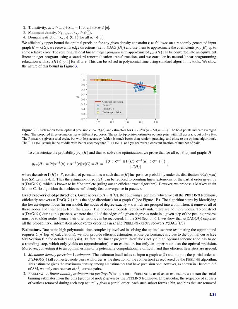
Robustness of the PEELING algorithm: Table 1 demonstrates robustness of our PEELING algorithm for various generaliza-tions of the model: preferential attachment model with variable m (denoted by M and ∼ unifa,b denote discrete uniformdistribution), uniform attachment model (denoted by UA ), and the more general Cooper-Frieze model20, 21. In our instance ofthe Cooper-Frieze model, the number of new edges m is drawn from ∼ unif5,50, the model allows either addition of a newnode (with probability 0.75) or addition of edges between existing nodes, and the endpoints of new edges can be selected eitherpreferentially (with probability 0.5) or uniformly among existing nodes. These results suggest that the proposed DAG-based
Technique θ(σpeel) ρ(σpeel) δ (σpeel)
PA (n,m = 25) 0.958 0.936 0.977PA (n,M), M ∼ unif5,50 0.691 0.683 0.988UA (n,m = 25) 0.977 0.967 0.99UA (n,M), M ∼ unif5,50 0.827 0.823 0.995Cooper-Frieze (Web graph) model 0.828 0.822 0.993
Table 1. A general comparison: n = 5000.methods can simultaneously achieve high precision and recall/density.
Real-world networks: We now discuss the performance of our estimators on several real-world networks, presented inTable 2 We first consider the ArXiv network as a directed network, with nodes corresponding to publications and edges fromeach publication to those that it cites. We also analyze the Simple English Wikipedia network – a directed graph showing thehyperlinks between articles of the Simple English Wikipedia. The DBLP computer science bibliography data is then modeledas an undirected network; an edge between two authors represents a joint publication. Finally, we study an SMS network andan online social network of Facebook focused on the New Orleans region, USA, with an edge (u,v, t) representing that user uposted on user v’s wall at time t. Results are presented in Table 2. For all of the networks tested, the methods described hereyield excellent precision and density.
Dataset # Nodes # Edges Genre θ(σpeel) ρ(σpeel) δ (σpeel) ρ(σpeel+)
ArXiv High Energy Physics 7.46K 116K Citation 0.708 0.681 0.961 0.707Simple English Wikipedia 100K 1.62M Hyperlink 0.624 0.548 0.878 0.609DBLP CS bibliography 1.13M 5.02M Coauthorship 0.785 0.728 0.927 0.764Facebook Wall post 43.9K 271K Social 0.698 0.657 0.941 0.687SMS network 30.2K 447K Social 0.669 0.610 0.912 0.621
Table 2. Results for real-world networks: A detailed description of the datasets are given in SM. θ(σpeel+)≈ ρ(σpeel+) and δ (σpeel+)≈ 1.When the density of the recovered partial order by PEELING algorithm is low, the recall can be improved via PEELING+ with a slight loss inprecision (see the Wikipedia result).
.
Figures 4 and 5 presents results of our analysis on human brain networks. The purpose here is to recover the evolutionaryorder among the important regions inside the brain. We note that there is no available ground truth (in terms of the network)for such ranking. Therefore our ranking provides important insight for further application studies. However, our rankingis “supported” by prior application studies14, 22, indicating that the brain network is well approximated by the preferentialattachment mechanism and its variations. We study two independent sets of brain networks of resting state fMRI images.The first one is derived from the Cambridge-Buckner dataset with 56 labeled brain regions. The PEELING estimator provides
6/31

a ranking of the brain regions; we analyze this ranking with respect to relatively sparse state of the art in our biologicalunderstanding of evolution of human brain. The corpus callosum, which joins the two hemispheres of the brain is believed tohave developed in the earliest stages of brain evolution, and the uncinate fasciculus, the white matter tract to have evolved latein the human brain. These observations are consistent with the rankings returned by our PEELING estimator. Our rankingsrepresent a first step towards determining the complete evolutionary trajectory of various regions of the brains.
The second network is extracted from the Human Connectome Project (HCP). We consider rankings of regions of 400networks from 100 individuals (2 session and 2 scans per subject), with more detailed 300 labeled regions in cortex. We plotthe histogram of arrival rank of prominent auditory, visual, and somatosensory regions. These histograms show a concentrationof rankings, indicating that our rankings are consistent among 100 people in the regions considered. Moreover, we observe thatmost of the regions that serve as prime functionaries among auditory, visual, and somatosensory regions have consistently lowarrival order in the 400 brain networks we analyzed. This is consistent with the widely accepted notion of early arrivals ofthese regions in the human brain evolution. Figure 5 illustrates the bins of brain regions of left hemisphere deduced with thePEELING estimator on a network generated from HCP data.
Figure 4. (A) PEELING bins of regions in Human brain network - Cambridge-Buckner. (B) Human Connectome brain data: histogram ofselected regions in cortex.
7/31

Figure 5. Illustration of the bins of prominent brain regions according to their arrival order in brain evolution: Inflated and flattenedrepresentation of left hemisphere of human brain. The network is formed from a correlation matrix of fMRI image of the data from HumanConnectome Project (See Methods for details). The borders and regions are defined according to the multi-modal parcellation techniqueproposed in23, and the figure is generated with Human Connectome Project’s workbench tools. The node (brain region) ranking given bythe PEELING algorithm are used to create batches of arrivals. The number indicated in the figure represents the first 22 bins, with bin 1corresponding to the bin of oldest nodes. Note that the primary visual cortex (V1) and primary auditory cortex (A1) are classified into olderbins. Code and data available at12
DiscussionWe focus here on node arrival inference from a single snapshot of a dynamic network. Our models, analyses framework, andmethods are applicable to a broad class of dynamic network generation models. Our infeasibility results (details in the SM) oftotal order recovery are useful in understanding fundamental limitations owing to different types of symmetries in networks.The general optimization problem we pose, which includes solutions of total and partial orders, provides an overarchingframework within which disparate algorithms can be evaluated. We use this framework to argue near-optimal solutions fromour estimators.
In a broader perspective, network archeology is not limited to the recovery of node arrival order, it generalizes to inferenceof higher order structures like triads, motifs, and communities. Our work provides the foundation for a rich class of problems inthe area, both from analytical and applications’ points of view. An alternate perspective of network archeology is in finding thecourse of (mis)information spreading. Recently, strategic information dissemination in online social networks like Twitter andFacebook has been alleged to create biases in opinions, even to the point of skewing electoral outcomes. Often, it is not onesingle source controlling the spread, rather, a group of nodes working in collusion. Our solutions provide powerful tools inidentifying and quarantining these malicious nodes rapidly.
Methods
Code and data availability. We make our code available at https://github.com/jithin-k-sreedharan/times.The code supports random graph model (variants of preferential attachment model) and real-world networks. It also includes ascript for generating brain networks from fMRI correlation data. The brain networks data is shared in the above link and theother networks used in this work are publicly available online. We solve the linear programming optimization using the Pythoninterface of a commercial optimizer Gurobi, and the script is available in the same link.
Constructing the brain networks. The data of Human Connectome project is the resting state fMRI data from HumanConnectome project focusing on the cortex area. The Human Connectome project provides a clean and refined data, whichgives consistent results in many published studies. We process and form brain networks out of 100 healthy young adults.First, the cortex brain data corresponding to 100 subjects (2 sessions per subject, and 2 scans per session) is parcellated into180 regions per hemisphere using a procedure described by Glasser et al.23 Then the correlation matrices are formed fromthe time series of the parcellated data. Finally binary, undirected networks are constructed from the correlation matrices asfollows: a spanning tree is created first from the complete network of the correlation matrix, and later k-nearest neighbors
8/31

(higher correlation values) of each node are added into this network, where k is chosen as 10 in our case. Each network has 300nodes, which are regions or clusters formed from group-Independent Component Analysis. The data is in correlation matrixformat, with each element as the Gaussianized version of the Pearson correlation coefficient (Fisher Z transform with AR(1)process estimation). In order to form a binary adjacency matrix, we use a threshold just high enough to make the resultinggraph connected. Such a graph is sparse.
Estimating pu,v using Markov chain Monte Carlo. We describe the procedure to estimate the integer programming coeffi-cients pu,v = pu,v(H) (Pr[π−1(u)< π−1(v)|π(G) = H]). Solving the original optimization requires knowledge of P = [pu,v],which can be estimated via MCMC (Markov chain Monte Carlo) techniques. The order of convergence of one importantMCMC technique (which we will call the Karzanov-Khachiyan algorithm and denote by K-K) for sampling uniformly fromthe set of linear extensions of a partial order, reported by24, is O(n6 log(n) log(1/ε)) transitions to achieve ε-bounded errorbetween the distribution of a sampled linear extension and the uniform distribution. Estimation of certain functions of theset of linear extensions in general requires more transitions. For instance, Brightwell and Winkler4 proved that estimatingthe total number of linear extensions based on K-K chain requires O(n9 log6(n)) transitions. From a practical, computationalperspective, this time complexity is untenable. Thus, we propose a different random walk (RW)-based algorithm.
First, a linear extension graph is formed as GLE = (VLE,ELE), where vertex set VLE consists of linear extensions Γ(H)consistent with the partial order (DAG) given by the DAG. The extensions λ and µ are adjacent in the graph if and only if λ
can be obtained from µ by an adjacent transposition. We describe a RW process below, which does not require the graph to beknown beforehand, instead the graph will be explored locally as neighbors of the nodes sampled by the random walk.
For instance, let v1,v2,v3,v4 be the nodes of the underlying PA graph. Let the partial order given by the DAG bev2 < v3 and v4 < v1. Then a node in the linear extension graph (which is a linear extension with the given partial order) isv4 < v1 < v2 < v3. Among the three possible adjacent transpositions of this total order, only one is a linear extension, which isv4 < v2 < v1 < v3. Thus the degree of this total order is 1. Figure 6 shows the graphs DAG(G) and GLE for this example.
Figure 6. An example DAG(G) and its linear extension graph GLE
The algorithm is as follows:
1. We sample a node λ in GLE, which is a linear extension, using the SEQUENTIAL algorithm (The SEQUENTIAL algorithmworks similar to the PEELING technique, but instead of peeling away all the m-degree nodes at each step, it removes onlya randomly selected node among the m-degree nodes present at any step and all other nodes stay for the next removal.).Let it be the initial node.
2. The neighbor set of λ can be obtained as follows. If any adjacent elements in λ form a perfect pair, they are not allowedto swap positions. All other adjacent pairs are allowed to transpose, and each neighbor of λ corresponds to a linearextension differed from λ with one transposed pair.
3. We run a simple random walk on graph GLE with the random walk choosing the next node in the walk uniformly amongthe neighbors of the present node.
4. Such a RW has a stationary distribution d(λ )/∑µ∈Γ(H) d(µ), where d(λ ) is the degree of linear extension λ in GLE. Weform the following ratio form estimator for Pu,v without directly unbiasing such a non-uniform distribution, which is
9/31

impossible without the knowledge of ∑µ∈Γ(H) d(µ).
p(k)u,v :=∑
kt=1 111Xt(u)< Xt(v)/d(Xt)
∑kt=1 1/d(Xt)
k→∞−−−→ |µ ∈ Γ(H) : µ(u)< µ(v)||Γ(H)| a.s.
Here Xt indicate the t-th sample of the RW, which is a linear extension of the underlying DAG.
5. Stop the RW when a convergence criteria is met.
Note that, unlike in K-K method, we do not need to make Markov chain aperiodic as the intention is not to sample from theunique stationary distribution, but only to estimate an average function of the nodes. The K-K method first forms a Markovchain similar to the construction in the above algorithm, but makes it aperidoc by adding self transitions with probability1−d(λ )/(2n−2). Given the discussion in SM Section 6.2.1, we expect d(λ ) should be very small, and hence the Markovchain in the K-K method spends a large amount of time in self loops, thus making the mixing slower. Our method avoidsartificial self loops, and achieves faster convergence in practice.
References1. Li, A., Cornelius, S. P., Liu, Y.-Y., Wang, L. & Barabási, A.-L. The fundamental advantages of temporal networks. Science
358, 1042–1046 (2017).
2. Pinney, J. W., Amoutzias, G. D., Rattray, M. & Robertson, D. L. Reconstruction of ancestral protein interaction networksfor the bzip transcription factors. Proc. Natl. Acad. Sci. 104, 20449–20453 (2007).
3. Srivastava, M. et al. The amphimedon queenslandica genome and the evolution of animal complexity. Nature 466, 720–726(2010).
4. Brightwell, G. & Winkler, P. Counting linear extensions. Order 8, 225–242 (1991).
5. Navlakha, S. & Kingsford, C. Network archaeology: Uncovering ancient networks from present-day interactions. PLOSComput. Biol. 7, 1–16 (2011).
6. Young, J.-G. et al. Network archaeology: phase transition in the recoverability of network history. arXiv preprintarXiv:1803.09191 (2018).
7. Bubeck, S., Devroye, L. & Lugosi, G. Finding adam in random growing trees. Random Struct. & Algorithms (2016).
8. Frieze, A., Pegden, W. et al. Looking for vertex number one. The Annals Appl. Probab. 27, 582–630 (2017).
9. Shah, D. & Zaman, T. Rumors in a network: Who’s the culprit? IEEE Transactions on information theory 57, 5163–5181(2011).
10. Zhu, K. & Ying, L. Information source detection in the sir model: A sample-path-based approach. IEEE/ACM Transactionson Netw. 24, 408–421 (2016).
11. Magner, A., Sreedharan, J. K., Grama, A. Y. & Szpankowski, W. Times: Temporal information maximally extracted fromstructures. In Proceedings of the 2018 World Wide Web Conference, WWW ’18, 389–398, DOI: 10.1145/3178876.3186105(2018).
12. Code & data of this submission. Available at https://github.com/jithin-k-sreedharan/times.
13. Barabási, A.-L. & Albert, R. Emergence of scaling in random networks. Science 286, 509–512 (1999).
14. Klimm, F., Bassett, D. S., Carlson, J. M. & Mucha, P. J. Resolving structural variability in network models and the brain.PLoS computational biology 10, e1003491 (2014).
15. Watts, D. J. The “new” science of networks. Annu. Rev. Sociol. 30, 243–270 (2004).
16. Perc, M. Evolution of the most common english words and phrases over the centuries. J. The Royal Soc. Interfacersif20120491 (2012).
17. Kunegis, J., Blattner, M. & Moser, C. Preferential attachment in online networks: Measurement and explanations. InProceedings of the 5th Annual ACM Web Science Conference, 205–214 (ACM, 2013).
18. Barabási, A.-L. et al. Evolution of the social network of scientific collaborations. Phys. A: Stat. mechanics its applications311, 590–614 (2002).
19. Barabási, A.-L. Network science: Luck or reason. Nature 489, 507 (2012).
20. Cooper, C. Distribution of vertex degree in web-graphs. Comb. Probab. Comput. 15, 637–661 (2006).
10/31

21. Cooper, C. & Frieze, A. A general model of web graphs. Random Struct. & Algorithms 22, 311–335 (2003).
22. Vértes, P. E. et al. Simple models of human brain functional networks. Proc. Natl. Acad. Sci. 109, 5868–5873 (2012).
23. Glasser, M. F. et al. A multi-modal parcellation of human cerebral cortex. Nature 536, 171–178 (2016).
24. Karzanov, A. & Khachiyan, L. On the conductance of order markov chains. Order 8, 7–15 (1991).
AcknowledgementsThis work was supported by NSF Center for Science of Information (CSoI) Grant CCF-0939370, NSF Grants CCF-1524312and CSR-1422338, and by NIH Grant 1U01CA198941-01. We thank Vikram Ravindra (Purdue) for the help in collecting thebrain data.
Author contributions statementAll authors designed and performed the research, and analyzed the results. J.S. implemented the methods and ran theexperiments. A.M performed the analytical calculations, and J.S. and W.S. assisted him. J.S. drafted the initial manuscript, andA.M., A.G. and W.S. edited and refined the manuscript. All authors read and approved the final manuscript.
Competing interestsThe authors declare that they have no competing interests.
11/31

Supplementary Material:Inferring Temporal Information from a Snapshot of a Dynamic
Network
Jithin Sreedharan†, Abram Magner†, Ananth Grama, and Wojciech Szpankowski∗
Center for Science of Information, Purdue University, USA∗To whom correspondence should be addressed
E-mail: [email protected]†Authors contributed equally.
February 3, 2019
Contents
1 Introduction 21.1 Overview of prior work . . . . . . . . . . . . . . . . . . . . . . . . . . . . . . . . . . . 2
2 Model and Definitions 2
3 Infeasibility of Total Order Recovery 33.1 Maximum likelihood estimation . . . . . . . . . . . . . . . . . . . . . . . . . . . . . . 6
4 Formulation and Solution of an Optimization Problem 74.1 Reduction of rational integer program to linear program . . . . . . . . . . . . . . . . 74.2 Coefficients of optimal precision . . . . . . . . . . . . . . . . . . . . . . . . . . . . . . 8
5 Optimal Solution for Preferential Attachment Graph Model 85.1 Recovering edge directions . . . . . . . . . . . . . . . . . . . . . . . . . . . . . . . . . 85.2 Integer program coefficients via Dir(H) . . . . . . . . . . . . . . . . . . . . . . . . . . 9
6 Algorithms and Estimators 106.1 Exact recovery of π(DAG(G)) . . . . . . . . . . . . . . . . . . . . . . . . . . . . . . . 106.2 Estimators and their properties . . . . . . . . . . . . . . . . . . . . . . . . . . . . . . 12
6.2.1 Maximum-density precision 1 estimator . . . . . . . . . . . . . . . . . . . . . 126.2.2 Peeling: A linear binning estimator via peeling . . . . . . . . . . . . . . . . 15
7 Experiments 157.1 Synthetic graphs . . . . . . . . . . . . . . . . . . . . . . . . . . . . . . . . . . . . . . 157.2 Real-world networks . . . . . . . . . . . . . . . . . . . . . . . . . . . . . . . . . . . . 16
7.2.1 Results . . . . . . . . . . . . . . . . . . . . . . . . . . . . . . . . . . . . . . . 18
1

1 Introduction
Throughout the supplementary information, we will generally follow certain notational conventions(unless otherwise stated), which we describe here. An arbitrary random graph model on n verticesis denoted by Gn, and a sample from that model by G. The random permutation generated by anadversary is given by π, and we use H to denote the observed graph π(G) (a random variable) orone of its possible values. Fixed graphs will generally be denoted by capital letters.
1.1 Overview of prior work
Mahantesh et al. [15] empirically studied inference of arrival order via a binning method. In thiscontext, we provide a rigorous formulation and analysis, a simpler solution without having to generatesamples from an estimated random graph model. We also provide a precise characterization of theperformance of our methods. To the best of our knowledge, our work presents the first feasible andrigorous approach to the problem of inferring partial orders in preferential attachment graphs. Wefirst formulated the present problem and presented some preliminary results in [14, 13].
For preferential attachment graphs, Frieze et al.[6] study the problem of identifying the oldestnode. However, their setting and goal are rather different: they assume that the arrival order ofnodes is known, and their goal is to arrive at the oldest node by a process that starts at a differentnode and only uses local information to advance.
2 Model and Definitions
The given formulation is equivalent to the following intuitive scenario: we are given a graph Gwith unique vertex ids, and there exists a hidden bijection ψ from the set of ids to the integers1, ..., n giving the order of arrival of the vertices, identified by their names. The task is to usethe structure of G to recover ψ. Formally, then, the problem that we study is entirely specified bythe following data: a distribution on labeled graphs (for the bulk of this paper, the preferentialattachment distribution PA(n,m), but in general denoted by Gn), the form that a solution takes,and a way of evaluating the performance of a given solution method.
To present succinctly our results we need three quantities associated with permutations of agraph model:
(a) Set of feasible permutations of a graph H: the subset Γ(H) ⊆ Sn, which consists of permuta-tions σ, such that σ(H) has positive probability under the distribution PA(n,m). An example of apermutation that is not feasible for a graph G generated by preferential attachment is π = (1, n),which swaps the first and last vertices. This is because the degree of the vertex labeled n in theresulting graph π(G) is > m, which happens with probability zero. We know that for this modelE[log |Γ(G)|] = n log n−O(n log logn) [11].
(b) Set of admissible graphs of H: Adm(H) = σ(H) : σ ∈ Γ(H). These are graphs obtainedby applying Γ(H) to H.
(c) Automorphism group: The automorphism group of a graph G, denoted by Aut(G), is the setof permutations π of vertices of G that preserve edge relations (i.e., the number of edges betweenvertices u and v is equal to the number of edges between vertices π(u) and π(v) in G). Note that|Adm(H)| = |Γ(H)|/|Aut(H)| [11].
2

3 Infeasibility of Total Order Recovery
Here we restrict the estimator to output a total order (i.e., a permutation) for which δ(σ) = 1. Anestimator function takes the form φ : Gn → Sn and Gn is the set of graphs on n vertices.
Let the minimax risk for a random graph model Gn be denoted by
R∗(Gn, d) = minφ
maxAn
E[d(φ(π(G)), π−1)],
where An is the the set of all adversaries, and d is some distortion measure on permutations. We focuson two natural choices for d, namely, error probability de(σ1, σ2) = I[σ1 6= σ2] for exact recovery,and Kendall τ distance τ(σ1, σ2) =
∑1≤i<j≤n I[σ2σ
−11 (i) > σ2σ
−11 (j)] for approximate recovery.
The next result says that, at least for the two distortion measures described above, the worst-caseadversary is the uniform distribution.
Theorem 3.1. In the case of error probability and Kendall τ distortion measures, we have, for anyadversary An, that the minimum risk over any estimator is greater than or equal to that for theadversary that chooses a permutation uniformly at random.
Proof. Consider an arbitrary adversary that outputs a permutation π on input G. We will construct arandomized estimator as follows: we draw uniformly at random a σ ∼ Sn and compute H ′ = σ(π(G)).Note that σ π is uniformly distributed on Sn. The estimator will then apply an optimal estimatorfor the uniform adversary to H ′, yielding a permutation λ, which is meant to be an approximationof (σ π)−1 = π−1 σ−1. Finally, the estimator outputs λσ as an approximation of π−1.
To analyze the precision of this estimator, we note the following chain of equalities holds, byelementary properties of the Kendall τ distance:
τ(λσ, π−1) = τ(λ, π−1σ−1) = τ(λ, (σπ)−1). (1)
Since (σπ)−1 is uniform on Sn and λ was generated by an optimal estimator for the uniform adversary,the expectation of the final expression is exactly equal to the minimum possible risk for the uniformadversary.
Finally, standard results yield that there exists a deterministic estimator with at least as largerisk, which concludes the proof. The derivation for the error probability distortion measure is similar,and we omit it.
The following theorem gives a general upper bound on the recall.
Theorem 3.2. Consider a random graph model Gn for which any two positive-probability isomorphicgraphs are equiprobable. Then the minimax risk is
R∗(Gn, de) ≥E[log |Aut(G)|] + E[log |Adm(G)|]− 1
log n!
=E[log |Γ(G)|]− 1
log n!.
Proof. We consider a particular adversary, one that chooses π uniformly at random from Sn. ApplyingFano’s inequality, we have that the probability of error is
Pr[φ(π(G)) 6= π−1] ≥ H(π−1|φ(π(G)))− 1
log |Sn|
=H(π−1|φ(π(G)))− 1
log n!
3

Now, by the data processing inequality and chain rule,
H(π−1|φ(π(G))) ≥ H(π−1|π(G))
= H(G|π(G)) +H(π−1|G, π(G)).
We note here that H(π−1|G, π(G)) = E[log |Aut(G)|] as there are exactly |Aut(G)| automorphismsbetween G and π(G), and H(G|π(G)) = E[log |Adm(G)|] since all isomorphic graphs with positiveprobability have the same probability.
For the preferential attachment model, the following lemma proves the assumption in Theorem 3.2.Strictly speaking, we prove the lemma for the version of the model in which vertex degrees areupdated with every connection choice. An approximate version holds under tweaks of the model(essentially because multiple edges are rare, and the results that rely on the lemma only require avery approximate version). In the proof and elsewhere throughout the supplementary information,we will use some common terms: a DAG is a directed, acyclic graph. The structure or unlabeledversion of a graph or a DAG M (denoted by S(M)) is the isomorphism class of the object in question(i.e., the set of all graphs or DAGs that are equivalent to the given one, up to permutations of itslabels).
Lemma 3.1. Consider two isomorphic preferential attachment graphs G1, G2 = σ(G1), σ ∈ Γ(G1).If Pr[G = G1] > 0, then
Pr[G = G1] = Pr[G = G2]. (2)
Proof. First, we will show that for a positive-probability graph K, Pr[G = K] depends only on theunlabeled DAG of K (see Definition 5.1 for the definition of the labeled version – namely, an edgefrom u to v exists in the (labeled) DAG of K if and only if u > v and there is an edge between uand v in K). Later in the supplementary information, we will state and prove Lemma 6.1, whichgives an algorithm for recovering the unlabeled DAG of K from the structure S(K), implying thatthe former is uniquely determined by the latter. This will complete the proof.
To show that Pr[G = K] depends only on the unlabeled DAG of K, we derive an explicitexpression as follows: for a given vertex v of K, denote the set of neighbors of v that chose vby NK(v). We call this set the parents of v. Furthermore, let d1(v) ≤ · · · ≤ dNK(v)(v) denotethe number of edges from each of the parents of v to v (note that all of this information is givenby the unlabeled DAG of K). Then we can write an expression for Pr[G = K] via the followingconsiderations: this probability is a ratio, the denominator of which is the product
∏mn−1j=1 (2mj).
This comes from the fact that for the jth connection choice made in the graph, the probability ofconnecting to any vertex contributes a denominator of 2mj. To determine an expression for thenumerator of Pr[G = K], we consider the contribution of vertex v, for arbitrary v with degree, say,d > m. When v joined the graph, it was given degree m. When a parent of v chooses to connectto v, bringing its degree from some d′ to d′ + 1, this contributes a factor of d′, leading to a factorof m(m + 1) · · · d = d!
(m−1)! . However, more is needed: a given parent that chooses v, say, di(v)
times can do so in(mdi(v)
)ways. More precisely, if a given vertex chooses to connect to ` vertices
a1, · · · , a` times, respectively, where a1 + · · ·+ a` = m, then there are(
ma1,··· ,a`
)ways to do this. In
the expression for the numerator of Pr[G = K], we will factor out the m! and associate the factor
4

1ai!
with its corresponding vertex (so 1di!
becomes associated with the vertex v). All of this leads tothe following expression:
Pr[G = K] =mn−1∏
j=1
(2mj)−1 × (m!)n−1×
∏
d>m
∏
v : degK(v)=d
d!
(m− 1)!
NK(v)∏
i=1
1
di!
Here, degK(v) denotes the degree of vertex v in the graph K. The product indexed by d is overall degrees > m present in the graph K, the product indexed by v is over all vertices having thegiven degree, and the one indexed by i is over all parents of v. Since all parts of this expression aredependent only on the structure of DAG(K), the lemma is proven.
In particular for preferential attachment graphs, we have the following inapproximability result.
Theorem 3.3. Let Gn denote PA(n,m), with m ≥ 3. Then we have R∗(Gn, de) = 1 − o(1).Furthermore, for approximate recovery, R∗(Gn, da) = Θ(n2). In other words, the recall is at most1−Θ(1), and thus no total order estimation algorithm can solve the problem without making a largenumber of inversion errors.
Proof. Recall that τ(·, ·) denotes the Kendall τ distance between two permutations.We will consider preferential attachment graphs, and will prove the bound for approximate
recovery, from which all other statements will follow. It is sufficient to exhibit an adversarydistribution for which the statement is true. We consider the set of degree-m nodes (denote this setby Dm(G)), which, with high probability, has size |Dm(G)| = Θ(n). Denote by SDm(G) the set ofpermutations in Sn which fix all vertices with degree not equal to m. Within this set, there is asubset R(G), with size tending to ∞ with n and such that any two permutations within R(G) haveKendall τ distance at least δ = cn2.
We consider an adversary that chooses π uniformly at random from R(G).Consider an arbitrary total order estimator φ. The intuition will be as follows: there are many
possible graph/permutation pairs (K, π) such that π(K) = π(G), and these π−1 are well-separated.So they must also be well-separated from φ(π(G)). This will provide the lower bound on the expectednumber of errors.
We start by conditioning on the value of π(G) and of π. Here, the outer sum is over all graphsK with at least c′n degree-m nodes, for some appropriate fixed c′ > 0.
E[τ(φ(π(G)), π−1)] ≥∑
K
Pr[π(G) = K]×∑
π∈R(K)
E[τ(φ(K), π−1)I[π = π] | π(G) = K].
The inner sum becomes∑
π∈R(K)
τ(φ(K), π−1)Pr[π = π | π(G) = K]. (3)
Now, the probability in this expression is simply 1/|R(K)|, which is constant with respect to π.
5

Thus, the inner sum further simplifies to
1
|R(K)|∑
π∈R(K)
τ(φ(K), π−1). (4)
To lower bound τ(φ(K), π−1) in this sum, denote by δmin the quantity
δmin = minσ∈R(K)
τ(φ(h), σ−1), (5)
and let σmin denote the optimizing permutation. Now, using the triangle inequality, we have
δ ≤ τ(π−1, σ−1min) ≤ τ(π−1, φ(K)) + τ(φ(K), σ−1
min)
= τ(π−1, φ(K)) + δmin.
We thus have, for all π ∈ R(K) not equal to σmin,
τ(π−1, φ(K)) ≥ maxδ − δmin, δmin. (6)
Then we have the following lower bound on (4).
1
|R(K)|∑
π∈R(K)
τ(φ(K), π−1) ≥ |R(K)| − 1
|R(K)| maxδ − δmin, δmin.
Now, we plug this in as a lower bound on the inner sum of (3), which gives
E[τ(φ(π(G)), π−1)]
≥∑
K
Pr[π(G) = K]|R(K)| − 1
|R(K)| maxδ − δmin, δmin.
The outer sum is again over the same set of graphs K as in (3).Now, in order to simplify the final expression, we recall that |R(K)| → ∞ as n → ∞, and
maxδ − δmin, δmin = Θ(n2). All of this gives
E[τ(φ(π(G)), π−1)] ≥ (1− o(1)) ·Θ(1) · n2 = Θ(n2). (7)
This immediately implies the desired upper bound on the precision/recall for the uniform distributionadversary.
We can prove the result for Erdős-Rényi by directly considering the uniform distribution adversary.The details are quite similar, so we omit them.
3.1 Maximum likelihood estimation
For the preferential attachment model, a natural way to approach the total order estimation problemis to frame it in terms of maximum likelihood estimation as follows: CML(H) = arg maxσ∈Sn
Pr[π−1 =σ|π(G) = H]. The following proposition proves that the optimal solution set CML gives a largenumber of equiprobable solutions and the maximum likelihood formulation is not a useful approachfor the problem.
6

Theorem 3.4. The maximum likelihood estimation solution set CML = CML(π(G)) satisfies |CML| =en logn−O(n log logn) with high probability.
Proof. First, by definition of Γ(H), we must have that CML(H) ⊆ Γ(H). We will show, in fact, thatthe likelihoods given to all elements of Γ(H) are equal. This will then imply that CML(H) = Γ(H).Next, from a result of [11], we have that with high probability |Γ(π(G))| = en logn−O(n log logn), whichwill complete the proof.
So it is sufficient to show that, for each σ ∈ Γ(H),
Pr[G = σ(H)|π(G) = H]
depends only on the structure S(H). To do this, note that by definition of Adm(H) and Γ(H), wemust have σ(H) ∈ Adm(H). So it is enough to show that for any two positive-probability isomorphicgraphs G1 and G2, we have Pr[G = G1] = Pr[G = G2]. This is the content of Lemma 3.1. Thiscompletes the proof of the proposition.
4 Formulation and Solution of an Optimization Problem
Remark 4.1. We could have defined a tradeoff curve between precision and recall, but this wouldhave the undesirable feature that the optimal precision is not necessarily defined for every value ofrecall in [0, 1], since some values for recall are not achievable [12].
4.1 Reduction of rational integer program to linear program
It is a general result that a rational linear program such as ours may be solved by converting to anequivalent truly linear program. We define a new variable s, which will capture the rational part ofthe objective function (i.e., we make the substitution s = 1/
∑1≤u6=v≤n xu,v, and yu,v = sxu,v). The
objective function is rewritten as a linear function of the normalized variables. This gives us the LPrelaxation
maxy,s
∑
1≤u<v≤npu,v(H)yu,v, (8)
subject to the constraints
1. yu,v ∈ [0, s],∀u, v ∈ [n]
2. 0 ≤ s ≤ 1
ε(n2
)
3. yu,v + yv,u ≤ s, ∀u, v ∈ [n]
4. yu,v + yv,w − yu,w ≤ s, ∀u, v, w ∈ [n]
5.∑
1≤u<v≤nyu,v = 1.
7

4.2 Coefficients of optimal precision
The integer program in the Main Text is rather explicit, except for the coefficient pu,v(H). The nextlemma gives a combinatorial formula for the probability pu,v(H).
Lemma 4.1 (Coefficients of the optimal precision). For all v, w ∈ [n] and graphs H, Pr[π−1(v) <
π−1(w)|π(G) = H] = |σ : σ−1∈Γ(H),σ−1(v)<σ−1(w)||Γ(H)| .
Proof. We can express the conditional probability in question as a sum, as follows:
Pr[π−1(v) < π−1(w)|π(G) = H]
=∑
σ : σ−1∈Γ(H)σ−1(v)<σ−1(w)
Pr[π = σ|π(G) = H]
Now, recall that π−1 ∈ Γ(H) under this conditioning, since π(G) = H and G is admissible.Moreover, it is uniformly distributed on Iso(G,H) (the set of isomorphisms from G to H), so wehave
Pr[π = σ|π(G) = H] =Pr[G = σ−1(H)|π(G) = H]
|Aut(H)|=
1
|Aut(H)||Adm(H)| .
Taking the sum, this becomes
|σ : σ−1 ∈ Γ(H), σ−1(v) < σ−1(w)||Aut(H)||Adm(H)| .
Finally, recall that |Adm(H)| = |Γ(H)|/|Aut(H)| [12].
5 Optimal Solution for Preferential Attachment Graph Model
From now on, we focus on the preferential attachment graph model, and solve the optimizationproblem explained in the previous section. In particular we describe how estimate pu,v(H). Later inthe section, we provide some efficient estimators that provide good approximations for the optimalsolution.
We remark that the existence of self-loops on the initial vertex in preferential attachment graphsallows for clean proofs; our theoretical and empirical results extend without significant changes tomodels in which these self-loops are not present.
5.1 Recovering edge directions
To efficiently calculate pu,v(H), we need to further characterize the set Γ(H) (note that its cardinalityis invariant under relabeling). At a high level, given H = π(G), we can recover a natural directed,acyclic version Dir(H), which induces a partial order on its vertices. We can then show that Γ(H) isprecisely the set of linear extensions [3] of this partial order. We can then use algorithms [2, 10]developed for approximate counting of linear extensions to estimate pu,v(H).
We first formalize the DAG in question:
8

Definition 5.1 (DAG of G). For G distributed according to the preferential attachment distribution(for any m), we define DAG(G) to be the directed acyclic graph defined on the same vertex set asG, such that there is an edge from u to v < u if and only if there is an edge between u and v in G.This is just G with the directions of edges marked in accordance with the graph evolution (leadingfrom younger nodes to older nodes).
We note here that DAG(G) and π(DAG(G)) are exactly the same in structure and relabelingwill not affect the directions, and we denote π(DAG(G)) by Dir(H).
5.2 Integer program coefficients via Dir(H)
The discussion in the previous subsection particularly implies that Γ(H) is precisely the set of linearextensions of the partial order defined by Dir(H).
Coming back to computing the coefficients pu,v(H) in the integer program, we see that thistask can be reduced to the problem of counting linear extensions of Dir(H) and of Dir(H) with theadditional relation that u ≺ v.
In full generality, the problem of counting linear extensions of an arbitrary partial order isclassically known to be #P-complete [4]. However, there exist fully polynomial-time approximationschemes for the problem, which allow us to approximate the coefficients up to an arbitrarily smallrelative error [8, 9].
Proposition 5.1. There exists a randomized algorithm which, on input H and positive number λ,outputs a sequence pu,v(H) satisfying |pu,v(H)−pu,v(H)| ≤ λpu,v(H) for all u, v ∈ [n] with probability1− o(1), in time
O(n5(log n)3λ−2 log(1/λ)).
The time complexity given in the above proposition is based on the worst case running times of thefastest known schemes [2, 10].
Given that we can approximate the coefficients pu,v(H) by pu,v(H) = (1± λ)pu,v(H) uniformlyfor arbitrarily small λ > 0, the next lemma bounds the effect of this approximation on the optimalvalue of the integer program.
Lemma 5.1. Consider the integer program whose objective function is given by Jε,λ(φ) =∑
1≤u<v≤n pu,v(H)xu,v∑1≤u6=v≤n xu,v
,
with the same constraints as in the original IP. Let φ∗ and φ∗ denote optimal points for the originaland modified integer programs, respectively. Then |Jε,λ(φ∗)− Jε(φ∗)| ≤ 3λ, for arbitrary λ > 0.
Proof. Our goal is to upper bound
|Jε(φ∗)− Jε,λ(φ∗)|.
We can rewrite this as
|Jε(φ∗)− Jε,λ(φ∗) + Jε,λ(φ∗)− Jε(φ∗) + Jε(φ∗)− Jε,λ(φ∗)|≤ |Jε,λ(φ∗)− Jε(φ∗)|+ |Jε,λ(φ∗)− Jε(φ∗)|+ |Jε,λ(φ∗)− Jε(φ∗)|
9

Now, the first and second differences on the right-hand side are at most λ, since
|Jε,λ(φ∗)− Jε(φ∗)|
≤∑
1≤u6=v≤n φ∗u,v|pu,v(H)− (1± λ)pu,v(H)|∑1≤u6=v≤n φ∗u,v
≤ λ∑
1≤u6=v≤n φ∗u,v∑1≤u6=v≤n φ∗u,v
= λ.
The remaining difference can be estimated as follows:
|Jε,λ(φ∗)− Jε(φ∗)|≤ max|Jε,λ(φ∗)− Jε(φ∗)|, |Jε,λ(φ∗)− Jε(φ∗)|≤ λ.
This inequality is a result of the fact that φ∗ and φ∗ are optimal points for their respective objectivefunctions. So we took the larger of Jε,λ(φ∗) and Jε(φ∗) and increased it, leading to the upper bound.
This shows that
|Jε(φ∗)− Jε,λ(φ∗)| ≤ 3λ,
so we only incur a small additive error in the optimal precision by estimating the coefficients.
Given these results, we can efficiently upper bound the optimal precision for any given densityconstraint as follows: on a randomly generated input graph H, we recover its edge directions (asexplained in the next section) and use them to approximate the coefficients pu,v(H) up to somerelative error λ. Now, at this point, we have a rational linear integer program with our approximationfor pu, v(H). We can convert this to an equivalent truly linear integer program using a standardrenormalization transformation and consider the natural linear programming relaxation, obtained byreplacing the binary constraint with xu,v(H) ∈ [0, 1] for all u, v. This can be solved in polynomialtime using standard tools.
6 Algorithms and Estimators
6.1 Exact recovery of π(DAG(G))
Next, we show that we can efficiently recover π(DAG(G)) for a preferential attachment graph G,given access to H = π(G), via a method that we call the Peeling technique. Recovering thedirections of edges from a younger node to an older node is the first step toward our goal. Thealgorithm starts by identifying the lowest-degree nodes (in our model, the nodes of degree exactlym) and we group them in a bin (group). Then, it removes all of these nodes and their edgesfrom the graph. Importantly, note that, in this step, all of the lowest-degree nodes are identifiedbefore any of them are removed, and all of the identified nodes are removed together. The processproceeds recursively, removing the lowest-degree nodes and placing them in a new bin, until thereare no more nodes to remove from the graph, as summarized in Algorithm 1 below. To constructDir(H) = π(DAG(G)) during this process, we simply note that all of the edges of a given degree-mnode in a given step of the peeling process must be to older nodes; hence, their orientations can berecovered (see Lemma 6.1).
10

Algorithm 1 Peeling Technique1: procedure Peeling(H)2: t← 13: while NoNodes(H) > 0 do . Finds no. of nodes4: MinDeg← FindMinDeg(H) . Finds minimum degree5: Bt ← u : deg(u) = MinDeg . Nodes with minimum degree6: H ← RemoveNodes(H,Bt) . Removes minimum degree nodes from H7: t← t+ 18: end while9: ReverseOrder(Bt) . Reverse the indices of Bt’s, e.g, 1 to t, t to 110: return Bt . Returns set of bins11: end procedure
Lemma 6.1. The Peeling algorithm exactly recovers π(DAG(G)) from π(G).
Proof. The Peeling algorithm maintains the following invariant at the beginning of each step: everydegree-m node connects only to vertices older than itself in the remaining graph. This is clear in theinitial step, since a node can only have degree exactly m in the full graph if its neighbors are allolder than it is. In subsequent steps (assuming by induction that the invariant holds for all previousones), if some edge incident with a degree-m node u is incident with a younger node v in the currentgraph, then this implies that some node w older than u and adjacent to u in a previous step hasalready been removed. This, in turn, implies that in that previous step, w had degree m and wasconnected to u, a younger vertex. This yields a contradiction, completing the proof.
The directed, acyclic graph π(DAG(G)) conveniently encodes the set of all vertex pairs whosetrue order relationship can be inferred with complete certainty. To make this precise, for a graph Hor the resulting DAG Dir(H), we define a vertex pair order event (u, v), for vertices u, v ∈ H, tobe simply an ordered pair of distinct vertices. We interpret this as a claim that u came before vaccording to π−1.
Definition 6.1. A vertex pair order event (u, v) is perfect for a graph H if, for all σ ∈ Γ(H), wehave σ(u) < σ(v). Equivalently, for any random permutation σ, Pr[σ−1(u) < σ−1(v)|σ(G) = H] = 1.
The following result formalizes our intuition that Dir(H) captures all probability-1 informationabout vertex ordering in H:
Theorem 6.1 (Dir(H) captures perfect vertex pair information). Consider a graph H on the vertexset [n] satisfying Γ(H) 6= ∅. Let its DAG Dir(H) be denoted by K. For any u, v ∈ [n], the pair (u, v)is perfect for H if and only if there exists a directed path in K from v to u (denoted by v u).
Proof. First, we will show that if v u, then (u, v) is perfect. This follows by showing the simplerclaim that if there is an edge from v to u (denoted by v → u), then (u, v) is perfect.
Let σ ∈ Γ(K). This means that σ(K) is a positive-probability DAG under the preferentialattachment model. Note also that σ(v)→ σ(u) in σ(K), which implies that we certainly must haveσ(v) > σ(u) (vertices only choose to connect to older vertices). Since σ was arbitrary, we have that(u, v) is perfect for H, as desired.
Now we show the converse claim: if (u, v) is perfect for K, then v u in K. We will do thisby proving the contrapositive: assume that there is no directed path from v to u. Then we will
11

construct a permutation σ satisfying i) σ ∈ Γ(K), and ii) σ(u) > σ(v). This is equivalent toproducing a feasible schedule of the vertices of K (i.e., a sequence of distinct vertices v1, v2, ..., vnof K, such that, for each j ∈ [n], all m of the the descendants of vj in K are contained in the setv1, ..., vj−1). We will require that vu > vv in the schedule. Such a schedule gives a permutationsatisfying the properties above as follows: for each j, σ(j) = vj .
To do this, we start by considering the sub-DAG Kv, consisting of v and all of its descendants.Now, we set v1 to be the bottom vertex of K (which is also the bottom vertex of Kv). We will addsubsequent vertices to our schedule as follows: at each time step t > 1, [n] is partitioned into threeparts: Sp,t (the vertices already in the schedule), Sa,t (the active vertices; i.e., those vertices notin Sp,t, all of whose children in K are contained in Sp,t), and Sd,t (the dormant vertices; i.e., thosevertices that are not active or already processed). So Sp,1 = v1, Sa,1 is the set of neighbors of v1,and Sd,1 consists of the rest of the vertices.
We observe that Sa,t is nonempty unless t = n: otherwise, there are less than n vertices in Sp,t(in fact, precisely t of them), and the rest are in Sd,t. In this case, consider the lowest vertex ` inSd,t; ` cannot have any children in Sd,t, since it is the lowest, so all of its children must be in Sp,t.But this means precisely that ` ∈ Sa,t. Thus, Sa,t must be nonempty.
Note that it is clear that at any time t, we can designate any active vertex as the next one in ourschedule; we would then move it to the processed set, potentially resulting in some vertices in Sd,tbecoming active.
Now, observe that at time t = 1, some vertex from Kv must be active (by the same reasoningthat established that the active set must be nonempty). In fact, until all vertices of Kv have beenprocessed, there remains at least one such vertex that is active. We thus choose active vertices Kv
until it is entirely processed (note that we do not process the vertex u /∈ Kv yet, since there is nodirected path from v to u). Then we process active vertices until a complete schedule has beengenerated. By construction, v comes earlier in the schedule than u, which completes the proof.
6.2 Estimators and their properties
Due to the high polynomial time complexity involved in solving the optimal scheme (Proposition 5.1and complexity of linear programming), we now provide efficient estimators whose performance isclose to the optimal curve. In fact, the linear program itself does not yield an optimal scheme (onehas to do a rounding step, which only yields an approximation) or an estimator, but only an upperbound on the optimal precision. Moreover, converting it to an optimal estimator is computationallydifficult and thus proposing efficient heuristics is warranted.
The time complexity of the estimators is dominated by the DAG construction, and is O(n log n).Note that one must take care in designing an estimator to ensure that the resulting set of vertex
pair order relations satisfies transitivity and antisymmetry.
6.2.1 Maximum-density precision 1 estimator
The estimator itself takes as input a graph H and outputs the partial order as Dir(H) as recoveredby the Peeling algorithm. This estimator gives the maximum density among all estimators thathave precision one.
In this subsection, we show that the point (density, precision) = (0, 1) is a point on the optimalprecision curve: namely, we prove that the perfect-precision estimator has precision one, butasymptotically negligible density, and this estimator has the maximum density among all precision
12

one estimators. From Theorem 6.1, we know that this achieves precision 1. So, in order to prove theremainder of our claim, we need to analyze the density of this estimator; that is, we analyze thetypical number of perfect pairs, culminating in the following theorem.
Theorem 6.2 (Typical number of perfect pairs). With high probability, for arbitrary fixed m ≥ 1,the number of perfect pairs associated with G is Ω(n log n) and o(n2) (uniformly in m). Whenm = 1, we have the matching upper bound of O(n log n), where the hidden constant in the asymptoticnotation can be explicitly calculated.
Proof. Upper bound: Let Xt denote the number of perfect pairs in the graph immediately aftertime t. We will prove the claimed upper bound by upper bounding Xt in expectation, then usingMarkov’s inequality. To bound E[Xt], we will show that it is sufficient to upper bound X(v) inexpectation for each v < t, where X(v) denotes the number of descendants of v in the DAG.
Using Proposition 1 of [11] with ` = Θ(log4/5 n log(log n)), we can show that the total number ofdescendants X(u), for all u ≤ n, is at most O(n/ log1/5 n), with high probability.
Now, we translate this to an upper bound on Xt as follows: we have E[Xt] ≤ E[Xt−1] + m +mO(t/ log1/5 t). This upper bound is from the following facts: at time t, all perfect vertex pairs fromtime t − 1 are still perfect, contributing the Xt−1 term. Next, vertex t makes at most m choices,creating at most m new perfect pairs (which explains the second term). Finally, the third termcomes from the fact that if t chooses v, and u is a descendant of v (so that (u, v) is a perfect pair),then (u, t) is also perfect.
Solving this recurrence, we find that E[Xt] = o(t2), as desired, and the proof is completed usingMarkov’s inequality.
In the case where m = 1, we have a much better upper bound on X(v), for arbitrary v: withhigh probability, at time t, X(v) = O(log t), as a result of the height of the tree being O(log t). Thisgives the improved bound of E[Xt] = O(t log t).
Lower bound: To prove the lower bound of Ω(t log t) perfect pairs, we write the total numberof perfect pairs in such a graph as the sum, over all vertices v ≤ t, of the number of descendantsX(v): Xt =
∑v≤tX(v).
In the m = 1 case (where G is a tree), this implies that Xt is the total path length of the tree.It is known that, with high probability, this parameter is Θ(t log t) (since it can be written as anadditive parameter, the results of [16] apply).
Now, to prove it for general m, we recall that to form a sample G from PA(n,m), we first producea sample T from PA(mn, 1), then collapse sequences ofm consecutive vertices. The number of perfectpairs in G is at least the same quantity in T , divided by m2, since there can be at most m2 edgesfrom one sequence of m consecutive vertices to an older sequence in T . Using the result for m = 1,we have that with high probability, the number of perfect pairs in T is Θ(mt log(mt)) = Θ(t log t),which implies that the number of perfect pairs in G is Ω(t log t).
The above theorem implies that the density of the perfect pair estimator is asymptotically 0, forarbitrary m. This is validated by simulation as shown in Figure 1. 1
Further scrutiny of the numerical evidence leads to a conjecture about the more precise behaviorof the number of perfect pairs as a function of m: we conjecture that for m > 1, the number ofperfect pairs is O(n1+δ(m)), for some function 1 > δ(m) > 0 (see again Figure 1).
1All simulation results take empirical expected values with respect to several samples from the graph distributionin question.
13

0 5000 10000 15000 20000 25000
no of nodes, n
0.000.050.100.150.200.250.300.350.400.45
#of
per
fect
pair
s/( n 2
)m = 1
m = 3
m = 5
(a) Upper bound
0 5000 10000 15000 20000 25000
no of nodes, n
02468
1012141618
#of
per
fect
pair
s/(n
log(n
))
m = 1
m = 3
(b) Lower bound
Figure 1: Normalizations of the number of perfect pairs in synthetic preferential attachment graphs.
This conjecture arises from the intuition from the (rigorous) proof of Theorem 6.2 as follows:denote by X(u) the number of descendants of any vertex u in DAG(G), and by Xt the number ofperfect pairs in the graph up to time t. If we can upper bound the number of descendants of anygiven vertex at time t by O(tc), for some constant c = c(m) < 1 dependent only on m (which issupported by empirical evidence), then we have E[Xt] ≤ E[Xt−1] +m+O(tc) = E[Xt−1] +O(tc).This upper bound arises as follows: the pairs that are perfect at time t− 1 remain perfect at timet, yielding the first term of the upper bound. The second and third terms arise from the fact thatvertex t connects to at most m other vertices (resulting in m additional perfect pairs), and eachperfect pair (v, w) involving two descendants of a node chosen by vertex t yields another perfect pair(v, t).
Iterating this recurrence and using Euler-Maclaurin summation, we find that E[Xt] = O(t1+c(m)),as desired. We give empirical evidence for the upper bound on X(t) (and hence for the improvedupper bound on the number of perfect pairs) in Figure 2, which indicates that the maximum numberof descendants of any node at a given time t is O(tc(m)).
0 2000 4000
no of nodes, n
0.7
0.8
0.9
log(a
vg.
#of
des
cendants
)lo
g(n
)
m = 5 m = 10 m = 15 m = 20 m = 25
0 2000 4000
no of nodes, n
0.80
0.85
0.90
0.95
log(m
ax.
#of
des
cendants
)lo
g(n
)
Figure 2: Normalized average and maximum number of descendants of degree-m nodes in DAG(G).
Theorem 6.2 gives us a single point on the optimal precision curve, and it is very simple to showthat the curve is decreasing as ε increases. In the next section, we show Peeling estimator achievesnontrivial density and precision with high probability, which gives a lower bound on the optimalprecision for another value of the density. We will use this to give an empirical indication of the
14

tightness of our upper bound.
6.2.2 Peeling: A linear binning estimator via peeling
When the term Peeling is used as an estimator, we mean the linear binning estimator2 from thebins (groups of nodes) given by the Peeling Algorithm 1. In particular, the sequence of subsets ofvertices removed during each step naturally gives a partial order: each such subset forms a bin, andbins that are removed earlier are considered to contain younger vertices.
We can start by showing a crude estimate of the precision and density of the Peeling estimator.
Theorem 6.3 (Non-negligible precision and density of the peeling estimator). For each m ≥ 1 thePeeling estimator has precision and density Θ(1).
Proof. The precision claim follows by showing that, with high probability, there exist Θ(n) verticesin the last Θ(n) timesteps that are never chosen (so that they are removed in the first bin and, thus,correctly declared to be younger than Θ(n) other vertices). This also proves the density claim.
The required result follows easily from the fact that with high probability there are Θ(n) verticesof degree m in the graph of size n. Namely, suppose that there are J degree-m vertices. We considerthe J/2th such vertex (say, vertex v). Then, clearly, since J/2 = Θ(n), we have that n− J/2 is alsoΘ(n), so that the result follows.
We now discuss further analysis of the procedure. In the case m = 1, the original graph G is atree, and we are able to precisely characterize certain parameters of the Peeling procedure, owingto the large amount of literature surrounding the preferential attachment distribution for this case(the structure is (essentially) identically distributed to a random plane-oriented recursive tree): forinstance, the asymptotic size of the jth youngest bin, for each fixed j, may be precisely determinedby writing it as an additive parameter and using results from Wagner et al. [16]. This gives us acomplicated but explicitly computable convergent series expression for the typical asymptotic densityof the estimator in this case. Precise theoretical results for m > 1 (and for the precision in them = 1 case) are much more elusive, owing to the fact that the precision and the DAG structureof the graph fail to lead to clean recursive formulas for parameters of interest (though a Pólya urnapproach allows us to derive very complicated expressions involving arbitrarily high moments andcovariances of quantities of interest); however, we can show that the peeling process recovers allperfect pairs, in addition to many imperfect ones.
7 Experiments
In this section, we evaluate our methods on synthetic and real-world networks. In what follows,σperf, σpeel, σpeel+ denote the partial orders produced by the Perfect-precision, Peeling, and Peel-ing+ algorithms.
7.1 Synthetic graphs
We derive significant insight by studying the Peeling method empirically. Table 1 and Figure 32A Linear binning is a special type of partial order, defined as follows: a partial order ≺ is a linear binning if its
elements may be partitioned into subsets B1, ...,Bj , for some j, such that u ≺ v if and only if there is a pair i < j suchthat u ∈ Bi and v ∈ Bj . This is equivalent to a graded partial order.
15
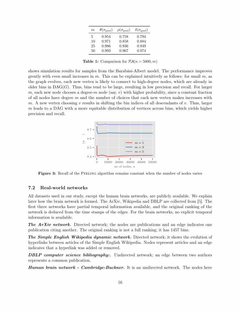
m θ(σpeel) ρ(σpeel) δ(σpeel)
5 0.954 0.758 0.79410 0.971 0.858 0.88425 0.986 0.936 0.94950 0.993 0.967 0.974
Table 1: Comparison for PA(n = 5000,m)
shows simulation results for samples from the Barabási-Albert model. The performance improvesgreatly with even small increases in m. This can be explained intuitively as follows: for small m, asthe graph evolves, each new vertex is likely to connect to high-degree nodes, which are already inolder bins in DAG(G). Thus, bins tend to be large, resulting in low precision and recall. For largerm, each new node chooses a degree-m node (say, v) with higher probability, since a constant fractionof all nodes have degree m and the number of choices that each new vertex makes increases withm. A new vertex choosing v results in shifting the bin indices of all descendants of v. Thus, largerm leads to a DAG with a more equitable distribution of vertices across bins, which yields higherprecision and recall.
0 10000 20000 30000 40000 50000
no of nodes, n
0.4
0.5
0.6
0.7
ρ(σ
peel)
m = 1
m = 3
m = 5
Figure 3: Recall of the Peeling algorithm remains constant when the number of nodes varies
7.2 Real-world networks
All datasets used in our study, except the human brain networks, are publicly available. We explainlater how the brain network is formed. The ArXiv, Wikipedia and DBLP are collected from [5]. Thefirst three networks have partial temporal information available, and the original ranking of thenetwork is deduced from the time stamps of the edges. For the brain networks, no explicit temporalinformation is available.
The ArXiv network. Directed network; the nodes are publications and an edge indicates onepublication citing another. The original ranking is not a full ranking; it has 1457 bins.
The Simple English Wikipedia dynamic network. Directed network; it shows the evolution ofhyperlinks between articles of the Simple English Wikipedia. Nodes represent articles and an edgeindicates that a hyperlink was added or removed.
DBLP computer science bibliography:. Undirected network; an edge between two authorsrepresents a common publication.
Human brain network - Cambridge-Buckner. It is an undirected network. The nodes here
16
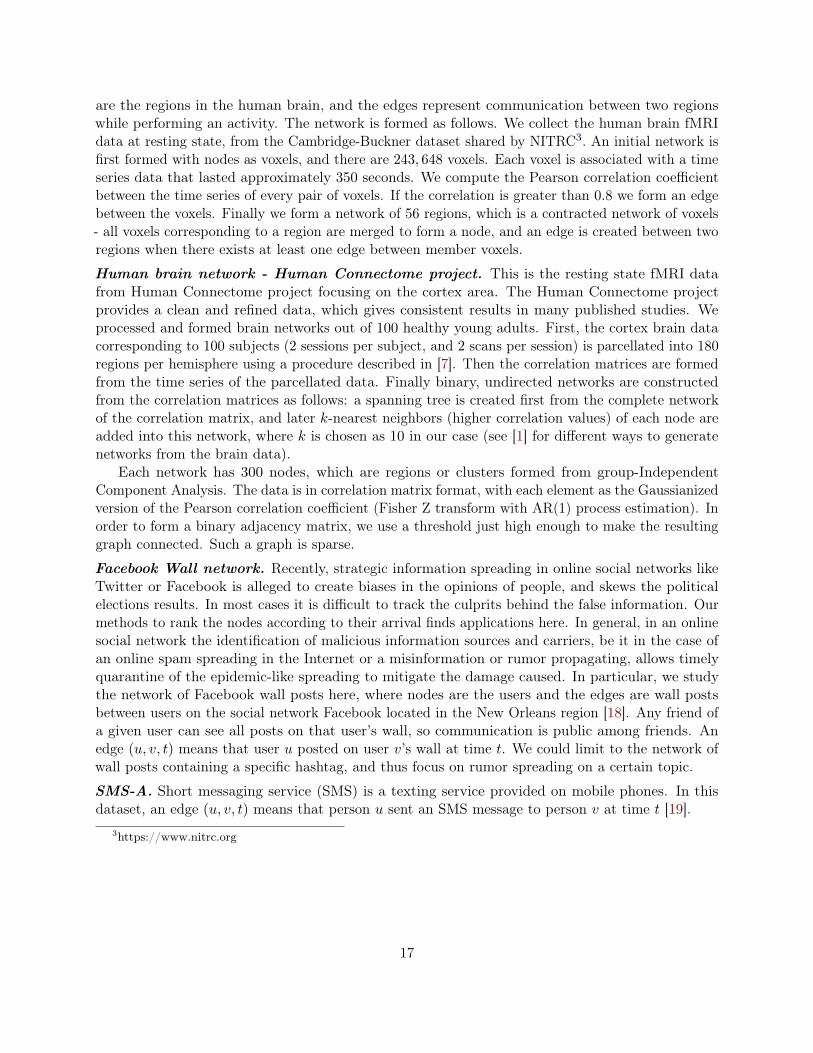
are the regions in the human brain, and the edges represent communication between two regionswhile performing an activity. The network is formed as follows. We collect the human brain fMRIdata at resting state, from the Cambridge-Buckner dataset shared by NITRC3. An initial network isfirst formed with nodes as voxels, and there are 243, 648 voxels. Each voxel is associated with a timeseries data that lasted approximately 350 seconds. We compute the Pearson correlation coefficientbetween the time series of every pair of voxels. If the correlation is greater than 0.8 we form an edgebetween the voxels. Finally we form a network of 56 regions, which is a contracted network of voxels- all voxels corresponding to a region are merged to form a node, and an edge is created between tworegions when there exists at least one edge between member voxels.
Human brain network - Human Connectome project. This is the resting state fMRI datafrom Human Connectome project focusing on the cortex area. The Human Connectome projectprovides a clean and refined data, which gives consistent results in many published studies. Weprocessed and formed brain networks out of 100 healthy young adults. First, the cortex brain datacorresponding to 100 subjects (2 sessions per subject, and 2 scans per session) is parcellated into 180regions per hemisphere using a procedure described in [7]. Then the correlation matrices are formedfrom the time series of the parcellated data. Finally binary, undirected networks are constructedfrom the correlation matrices as follows: a spanning tree is created first from the complete networkof the correlation matrix, and later k-nearest neighbors (higher correlation values) of each node areadded into this network, where k is chosen as 10 in our case (see [1] for different ways to generatenetworks from the brain data).
Each network has 300 nodes, which are regions or clusters formed from group-IndependentComponent Analysis. The data is in correlation matrix format, with each element as the Gaussianizedversion of the Pearson correlation coefficient (Fisher Z transform with AR(1) process estimation). Inorder to form a binary adjacency matrix, we use a threshold just high enough to make the resultinggraph connected. Such a graph is sparse.
Facebook Wall network. Recently, strategic information spreading in online social networks likeTwitter or Facebook is alleged to create biases in the opinions of people, and skews the politicalelections results. In most cases it is difficult to track the culprits behind the false information. Ourmethods to rank the nodes according to their arrival finds applications here. In general, in an onlinesocial network the identification of malicious information sources and carriers, be it in the case ofan online spam spreading in the Internet or a misinformation or rumor propagating, allows timelyquarantine of the epidemic-like spreading to mitigate the damage caused. In particular, we studythe network of Facebook wall posts here, where nodes are the users and the edges are wall postsbetween users on the social network Facebook located in the New Orleans region [18]. Any friend ofa given user can see all posts on that user’s wall, so communication is public among friends. Anedge (u, v, t) means that user u posted on user v’s wall at time t. We could limit to the network ofwall posts containing a specific hashtag, and thus focus on rumor spreading on a certain topic.
SMS-A. Short messaging service (SMS) is a texting service provided on mobile phones. In thisdataset, an edge (u, v, t) means that person u sent an SMS message to person v at time t [19].
3https://www.nitrc.org
17
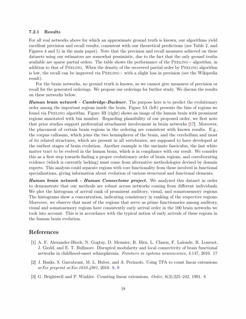
7.2.1 Results
For all real networks above for which an approximate ground truth is known, our algorithms yieldexcellent precision and recall results, consistent with our theoretical predictions (see Table 2, andFigures 4 and 5) in the main paper). Note that the precision and recall measures achieved on thesedatasets using our estimators are somewhat pessimistic, due to the fact that the only ground truthsavailable are sparse partial orders. The table shows the performance of the Peeling+ algorithm, inaddition to that of Peeling. When the density of the recovered partial order by Peeling algorithmis low, the recall can be improved via Peeling+ with a slight loss in precision (see the Wikipediaresult).
For the brain networks, no ground truth is known, so we cannot give measures of precision orrecall for the generated orderings. We propose our orderings for further study. We discuss the resultson these networks below.
Human brain network - Cambridge-Buckner. The purpose here is to predict the evolutionaryorder among the important regions inside the brain. Figure 3A (left) presents the bins of regions wefound via Peeling algorithm. Figure 3B (right) shows an image of the human brain with prominentregions annotated with bin number. Regarding plausibility of our proposed order, we first notethat prior studies support preferential attachment involvement in brain networks [17]. Moreover,the placement of certain brain regions in the ordering are consistent with known results. E.g.,the corpus callosum, which joins the two hemispheres of the brain, and the cerebellum and mostof its related structures, which are present in all vertebrates, are supposed to have developed atthe earliest stages of brain evolution. Another example is the uncinate fasciculus, the last whitematter tract to be evolved in the human brain, which is in compliance with our result. We considerthis as a first step towards finding a proper evolutionary order of brain regions, and corroboratingevidence (which is currently lacking) must come from alternative methodologies devised by domainexperts. This analysis could separate regions with core functionality from those involved in functionalspecializations, giving information about evolution of various structural and functional elements.
Human brain network - Human Connectome project. We analyzed this dataset in orderto demonstrate that our methods are robust across networks coming from different individuals.We plot the histogram of arrival rank of prominent auditory, visual, and somatosensory regions.The histograms show a concentration, indicating consistency in ranking of the respective regions.Moreover, we observe that most of the regions that serve as prime functionaries among auditory,visual and somatosensory regions have consistently early arrival order in the 100 brain networks wetook into account. This is in accordance with the typical notion of early arrivals of these regions inthe human brain evolution.
References
[1] A. F. Alexander-Bloch, N. Gogtay, D. Meunier, R. Birn, L. Clasen, F. Lalonde, R. Lenroot,J. Giedd, and E. T. Bullmore. Disrupted modularity and local connectivity of brain functionalnetworks in childhood-onset schizophrenia. Frontiers in systems neuroscience, 4:147, 2010. 17
[2] J. Banks, S. Garrabrant, M. L. Huber, and A. Perizzolo. Using TPA to count linear extensions.arXiv preprint arXiv:1010.4981, 2010. 8, 9
[3] G. Brightwell and P. Winkler. Counting linear extensions. Order, 8(3):225–242, 1991. 8
18

[4] G. Brightwell and P. Winkler. Counting linear extensions is #p-complete. In Proceedings of theTwenty-third Annual ACM Symposium on Theory of Computing (STOC), pages 175–181, NewYork, NY, USA, 1991. ACM. 9
[5] K. T. K. N. Collection. Preferential attachment exponent. Available on http://konect.uni-koblenz.de/statistics/prefatt [Accessed: 30 April 2017], 2016. 16
[6] A. Frieze, W. Pegden, et al. Looking for vertex number one. The Annals of Applied Probability,27(1):582–630, 2017. 2
[7] M. F. Glasser, T. S. Coalson, E. C. Robinson, C. D. Hacker, J. Harwell, E. Yacoub, K. Ugurbil,J. Andersson, C. F. Beckmann, M. Jenkinson, et al. A multi-modal parcellation of humancerebral cortex. Nature, 536(7615):171–178, 2016. 17
[8] M. Huber. Fast perfect sampling from linear extensions. Discrete Mathematics, 306(4):420–428,2006. 9
[9] M. R. Jerrum, L. G. Valiant, and V. V. Vazirani. Random generation of combinatorial structuresfrom a uniform distribution. Theoretical Computer Science, 43:169–188, 1986. 9
[10] A. Karzanov and L. Khachiyan. On the conductance of order markov chains. Order, 8(1):7–15,1991. 8, 9
[11] T. Łuczak, A. Magner, and W. Szpankowski. Asymmetry and structural information inpreferential attachment graphs. Random Structures & Algorithms (to appear); arXiv preprintarXiv:1607.04102, 2019. 2, 7, 13
[12] A. Magner, A. Grama, J. Sreedharan, and W. Szpankowski. Recovery of vertex orderings indynamic graphs. In Proceedings of the IEEE International Symposium on Information Theory(ISIT), 2017. 7, 8
[13] A. Magner, A. Grama, J. K. Sreedharan, and W. Szpankowski. Recovery of vertex orderings indynamic graphs. In 2017 IEEE International Symposium on Information Theory (ISIT), pages1563–1567, June 2017. 2
[14] A. Magner, J. K. Sreedharan, A. Y. Grama, and W. Szpankowski. Times: Temporal informationmaximally extracted from structures. In Proceedings of the 2018 World Wide Web Conference,WWW ’18, pages 389–398, 2018. 2
[15] S. M. V. Mahantesh, S. Iyengar, M. Vijesh, S. R. Nayak, and N. Shenoy. Prediction of arrival ofnodes in a scale free network. In Proceedings of the 2012 International Conference on Advancesin Social Networks Analysis and Mining (ASONAM), pages 517–521, 2012. 2
[16] D. Ralaivaosaona and S. Wagner. Additive functionals of d-ary increasing trees. In Proceedingsof the 27th International Conference on Probabilistic, Combinatorial, and Asymptotic Methodsfor the Analysis of Algorithms, pages 1–12, 2016. 13, 15
[17] P. E. Vértes, A. F. Alexander-Bloch, N. Gogtay, J. N. Giedd, J. L. Rapoport, and E. T. Bullmore.Simple models of human brain functional networks. Proceedings of the National Academy ofSciences, 109(15):5868–5873, 2012. 18
19

[18] B. Viswanath, A. Mislove, M. Cha, and K. P. Gummadi. On the evolution of user interactionin facebook. In Proceedings of the 2nd ACM workshop on Online social networks, pages 37–42.ACM, 2009. 17
[19] Y. Wu, C. Zhou, J. Xiao, J. Kurths, and H. J. Schellnhuber. Evidence for a bimodal distributionin human communication. Proceedings of the national academy of sciences, 107(44):18803–18808,2010. 17
20