10/25/2000 4

Inferring rudimentary rules� 1R: learns a 1-level decision tree

� In other words, generates a set of rules that all test on one particular attribute

� Basic version (assuming nominal attributes)

� One branch for each of the attribute’s values

� Each branch assigns most frequent class

� Error rate: proportion of instances that don’t belong to the majority class of their corresponding branch

� Choose attribute with lowest error rate

10/25/2000 5

Pseudo-code for 1R

For each attribute,

For each value of the attribute, make a rule as follows:

count how often each class appears

find the most frequent class

make the rule assign that class to this attribute-value

Calculate the error rate of the rules

Choose the rules with the smallest error rate

� Note: “missing” is always treated as a separate attribute value

10/25/2000 6

Evaluating the weather attributes

3/6True → No*

5/142/8False → YesWindy

1/7Normal → Yes

4/143/7High → NoHumidity

5/14

4/14

Total errors

1/4Cool → Yes

2/6Mild → Yes

2/4Hot → No*Temperature

2/5Rainy → Yes

0/4Overcast → Yes

2/5Sunny → NoOutlook

ErrorsRulesAttribute

NoTrueHighMildRainy

YesFalseNormalHotOvercast

YesTrueHighMildOvercast

YesTrueNormalMildSunny

YesFalseNormalMildRainy

YesFalseNormalCoolSunny

NoFalseHighMildSunny

YesTrueNormalCoolOvercast

NoTrueNormalCoolRainy

YesFalseNormalCoolRainy

YesFalseHighMildRainy

YesFalseHighHot Overcast

NoTrueHigh Hot Sunny

NoFalseHighHotSunny

PlayWindyHumidityTemp.Outlook

10/25/2000 7

Dealing with numeric attributes� Numeric attributes are discretized: the range of the

attribute is divided into a set of intervals

� Instances are sorted according to attribute’s values

� Breakpoints are placed where the (majority) class changes (so that the total error is minimized)

� Example: temperature from weather data

64 65 68 69 70 71 72 72 75 75 80 81 83 85Yes | No | Yes Yes Yes | No No Yes | Yes Yes | No | Yes Yes | No

10/25/2000 8

The problem of overfitting� Discretization procedure is very sensitive to noise

� A single instance with an incorrect class label will most likely result in a separate interval

� Also: time stamp attribute will have zero errors

� Simple solution: enforce minimum number of instances in majority class per interval

� Weather data example (with minimum set to 3):64 65 68 69 70 71 72 72 75 75 80 81 83 85Yes | No | Yes Yes Yes | No No Yes | Yes Yes | No | Yes Yes | No

10/25/2000 9

Result of overfitting avoidance� Final result for for temperature attribute:

� Resultingrule sets:

64 65 68 69 70 71 72 72 75 75 80 81 83 85Yes No Yes Yes Yes | No No Yes Yes Yes | No Yes Yes No

0/1> 95.5 → Yes

3/6True → No*

5/142/8False → YesWindy

2/6> 82.5 and ≤ 95.5 → No

3/141/7≤ 82.5 → YesHumidity

5/14

4/14

Total errors

2/4> 77.5 → No*

3/10≤ 77.5 → YesTemperature

2/5Rainy → Yes

0/4Overcast → Yes

2/5Sunny → NoOutlook

ErrorsRulesAttribute

10/25/2000 10

Discussion of 1R� 1R was described in a paper by Holte (1993)

Contains an experimental evaluation on 16 datasets (using cross-validation so that results were representative of performance on future data)

Minimum number of instances was set to 6 after some experimentation

1R’s simple rules performed not much worse than much more complex decision trees

� Simplicity first pays off!

10/25/2000 24

Constructing decision trees Normal procedure: top down in recursive divide-

and-conquer fashion

� First: attribute is selected for root node and branch is created for each possible attribute value

� Then: the instances are split into subsets (one for each branch extending from the node)

� Finally: procedure is repeated recursively for each branch, using only instances that reach the branch

Process stops if all instances have the same class

10/25/2000 25

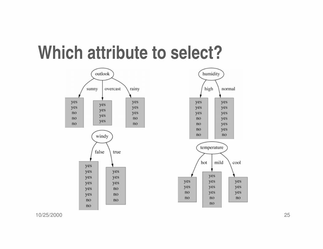
Which attribute to select?

10/25/2000 26

A criterion for attribute selection� Which is the best attribute?

The one which will result in the smallest tree

Heuristic: choose the attribute that produces the “purest” nodes

� Popular impurity criterion: information gain

Information gain increases with the average purity of the subsets that an attribute produces

� Strategy: choose attribute that results in greatest information gain

10/25/2000 27

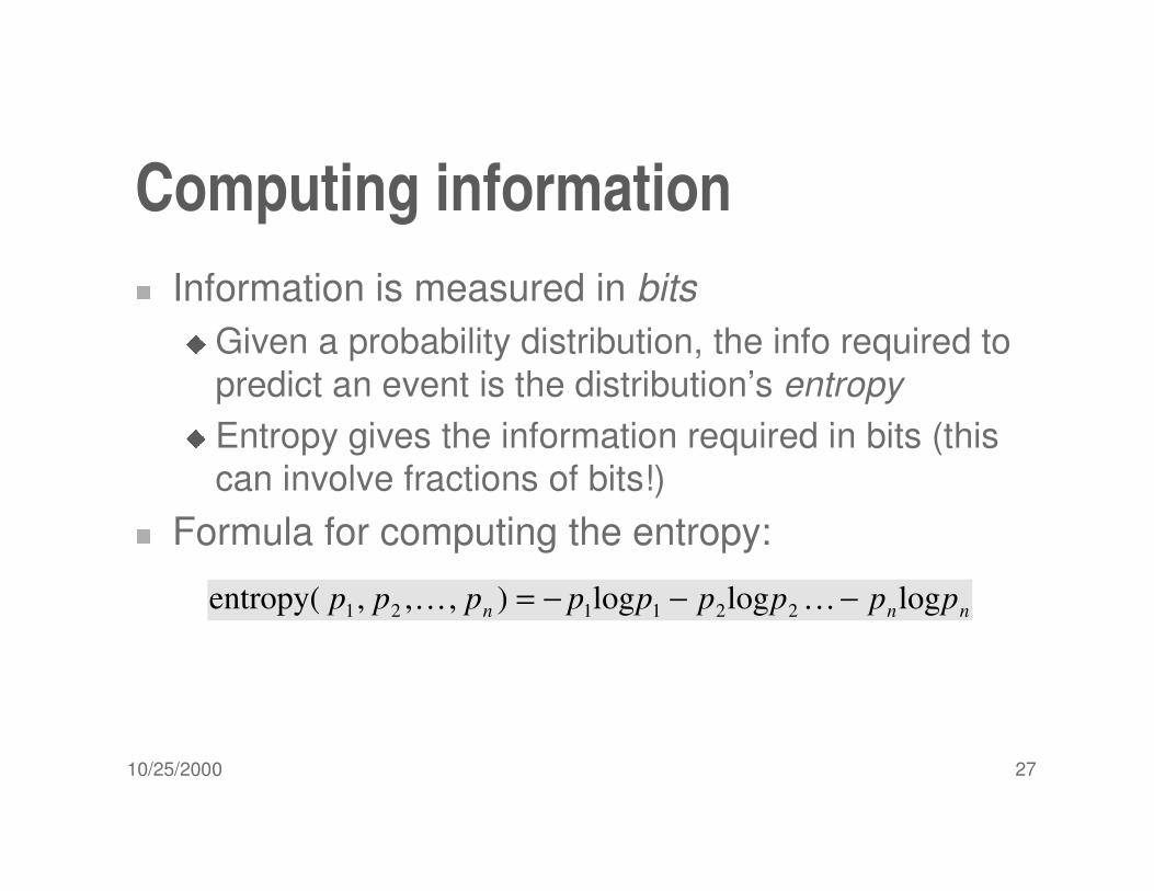
Computing information� Information is measured in bits

� Given a probability distribution, the info required to predict an event is the distribution’s entropy

� Entropy gives the information required in bits (this can involve fractions of bits!)

� Formula for computing the entropy:

nnn ppppppppp logloglog),,,entropy( 221121 −−−= ��

10/25/2000 28

Example: attribute “Outlook” � “Outlook” = “Sunny”:

� “Outlook” = “Overcast”:

� “Outlook” = “Rainy”:

� Expected information for attribute:

bits 971.0)5/3log(5/3)5/2log(5/25,3/5)entropy(2/)info([2,3] =−−==

bits 0)0log(0)1log(10)entropy(1,)info([4,0] =−−==

bits 971.0)5/2log(5/2)5/3log(5/35,2/5)entropy(3/)info([3,2] =−−==

Note: this isnormally notdefined.

971.0)14/5(0)14/4(971.0)14/5([3,2])[4,0],,info([3,2] ×+×+×=bits 693.0=

10/25/2000 29

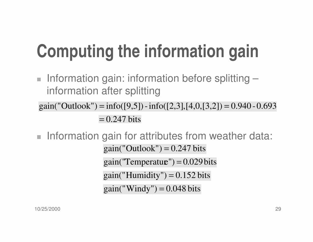
Computing the information gain� Information gain: information before splitting –

information after splitting

� Information gain for attributes from weather data:

0.693-0.940[3,2])[4,0,,info([2,3]-)info([9,5])Outlook"gain(" ==bits 247.0=

bits 247.0)Outlook"gain(" =bits 029.0)e"Temperaturgain(" =

bits 152.0)Humidity"gain(" =bits 048.0)Windy"gain(" =

10/25/2000 30

Continuing to split

bits 571.0)e"Temperaturgain(" =bits 971.0)Humidity"gain(" =

bits 020.0)Windy"gain(" =

10/25/2000 31

The final decision tree� Note: not all leaves need to be pure; sometimes

identical instances have different classes⇒ Splitting stops when data can’t be split any further

10/25/2000 32

Wishlist for a purity measure� Properties we require from a purity measure:

� When node is pure, measure should be zero

� When impurity is maximal (i.e. all classes equally likely), measure should be maximal

� Measure should obey multistage property (i.e. decisions can be made in several stages):

� Entropy is the only function that satisfies all three properties!

,4])measure([3(7/9),7])measure([2,3,4])measure([2 ×+=

10/25/2000 33

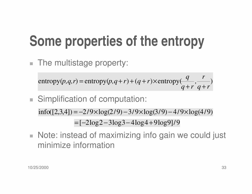
Some properties of the entropy� The multistage property:

� Simplification of computation:

� Note: instead of maximizing info gain we could just minimize information

)entropy()()entropy()entropy(rq

r,

rqq

rqrp,qp,q,r++

×+++=

)9/4log(9/4)9/3log(9/3)9/2log(9/2])4,3,2([info ×−×−×−=9/]9log94log43log32log2[ +−−−=

10/25/2000 34

Highly-branching attributes� Problematic: attributes with a large number of

values (extreme case: ID code)

� Subsets are more likely to be pure if there is a large number of values

⇒ Information gain is biased towards choosing attributes with a large number of values

⇒ This may result in overfitting (selection of an attribute that is non-optimal for prediction)

� Another problem: fragmentation

10/25/2000 35

The weather data with ID code

N

M

L

K

J

I

H

G

F

E

D

C

B

A

ID code

NoTrueHighMildRainy

YesFalseNormalHotOvercast

YesTrueHighMildOvercast

YesTrueNormalMildSunny

YesFalseNormalMildRainy

YesFalseNormalCoolSunny

NoFalseHighMildSunny

YesTrueNormalCoolOvercast

NoTrueNormalCoolRainy

YesFalseNormalCoolRainy

YesFalseHighMildRainy

YesFalseHighHot Overcast

NoTrueHigh Hot Sunny

NoFalseHighHotSunny

PlayWindyHumidityTemp.Outlook

10/25/2000 36

Tree stump for ID code attribute� Entropy of split:

⇒ Information gain is maximal for ID code (namely 0.940 bits)

bits 0)info([0,1])info([0,1])info([0,1])code" ID"(info =+++= �

10/25/2000 37

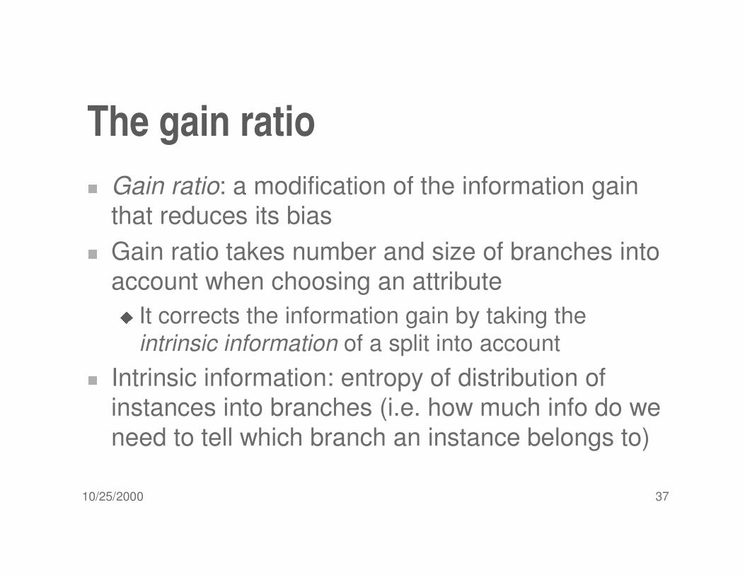
The gain ratio� Gain ratio: a modification of the information gain

that reduces its bias

� Gain ratio takes number and size of branches into account when choosing an attribute

� It corrects the information gain by taking the intrinsic information of a split into account

� Intrinsic information: entropy of distribution of instances into branches (i.e. how much info do we need to tell which branch an instance belongs to)

10/25/2000 38

Computing the gain ratio� Example: intrinsic information for ID code

� Value of attribute decreases as intrinsic information gets larger

� Definition of gain ratio:

� Example:

bits 807.3)14/1log14/1(14),1[1,1,(info =×−×=�

)Attribute"info("intrinsic_)Attribute"gain("

)Attribute"("gain_ratio =

246.0bits 3.807bits 0.940

)ID_code"("gain_ratio ==

10/25/2000 39

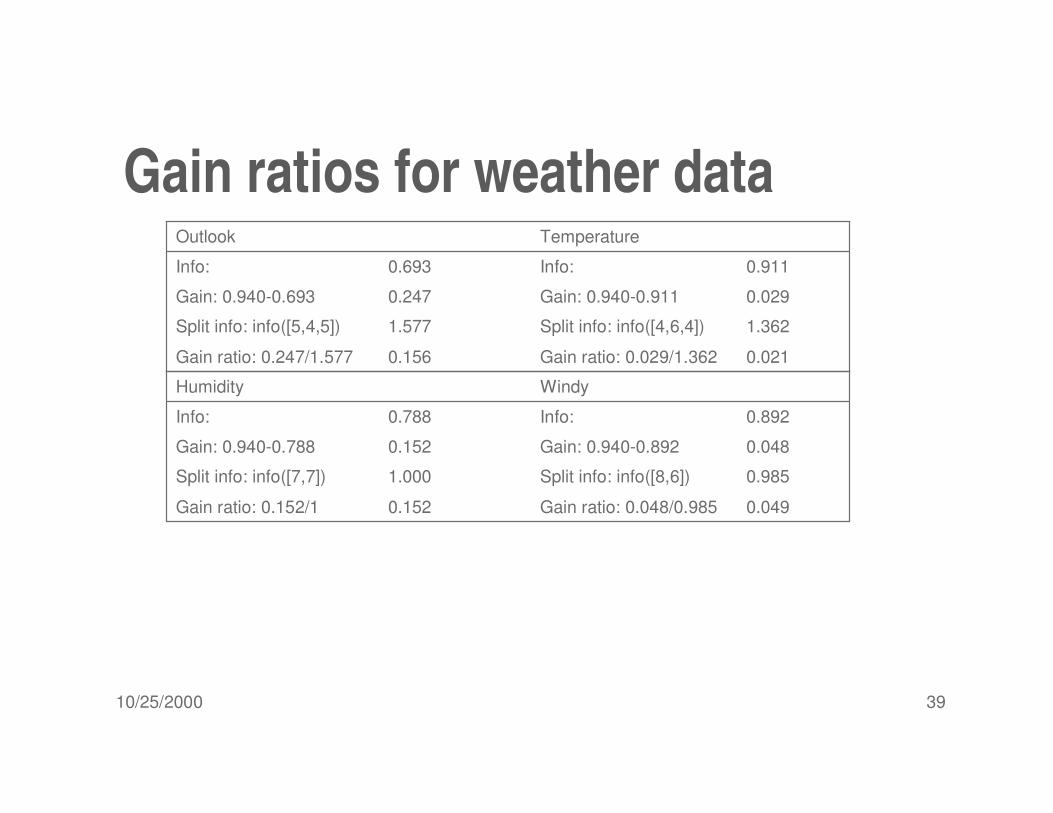
Gain ratios for weather data

0.021Gain ratio: 0.029/1.3620.156Gain ratio: 0.247/1.577

1.362Split info: info([4,6,4])1.577 Split info: info([5,4,5])

0.029Gain: 0.940-0.911 0.247 Gain: 0.940-0.693

0.911Info:0.693Info:

TemperatureOutlook

0.049Gain ratio: 0.048/0.9850.152Gain ratio: 0.152/1

0.985Split info: info([8,6])1.000 Split info: info([7,7])

0.048Gain: 0.940-0.892 0.152Gain: 0.940-0.788

0.892Info:0.788Info:

WindyHumidity

10/25/2000 40

More on the gain ratio� “Outlook” still comes out top

� However: “ID code” has greater gain ratio

� Standard fix: ad hoc test to prevent splitting on that type of attribute

� Problem with gain ratio: it may overcompensate

� May choose an attribute just because its intrinsic information is very low

� Standard fix: only consider attributes with greater than average information gain

10/25/2000 41

Discussion� Algorithm for top-down induction of decision trees

(“ID3”) was developed by Ross Quinlan

� Gain ratio just one modification of this basic algorithm

� Led to development of C4.5, which can deal with numeric attributes, missing values, and noisy data

� Similar approach: CART

� There are many other attribute selection criteria! (But almost no difference in accuracy of result.)

10/25/2000 42

Covering algorithms� Decision tree can be converted into a rule set

Straightforward conversion: rule set overly complex

More effective conversions are not trivial

� Strategy for generating a rule set directly: for each class in turn find rule set that covers all instances in it (excluding instances not in the class)

� This approach is called a covering approach because at each stage a rule is identified that covers some of the instances

10/25/2000 43

Example: generating a rule

y

x

a

b b

b

b

b

bb

b

b b bb

bb

a aaa

ay

a

b b

b

b

b

bb

b

b b bb

bb

a aaa

a

x1·2

y

a

b b

b

b

b

bb

b

b b bb

bb

a aaa

a

x1·2

2·6

If x > 1.2 then class = a

If x > 1.2 and y > 2.6 then class = aIf true then class = a

! Possible rule set for class “b”:

! More rules could be added for “perfect” rule set

If x ≤ 1.2 then class = b

If x > 1.2 and y ≤ 2.6 then class = b

10/25/2000 44

Rules vs. trees" Corresponding decision tree:

(produces exactly the samepredictions)

" But: rule sets can be more perspicuous when decision trees suffer from replicated subtrees

" Also: in multiclass situations, covering algorithm concentrates on one class at a time whereas decision tree learner takes all classes into account

10/25/2000 45

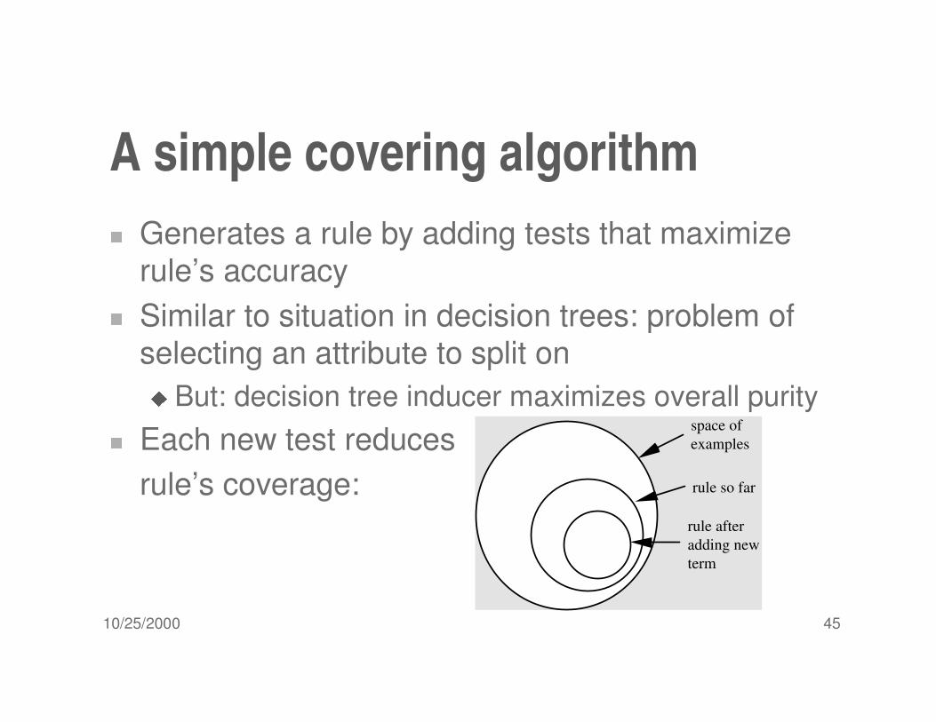
A simple covering algorithm# Generates a rule by adding tests that maximize

rule’s accuracy

# Similar to situation in decision trees: problem of selecting an attribute to split on

$ But: decision tree inducer maximizes overall purity

# Each new test reducesrule’s coverage:

space of examples

rule so far

rule after adding new term

10/25/2000 46

Selecting a test% Goal: maximizing accuracy

& t: total number of instances covered by rule

& p: positive examples of the class covered by rule

& t-p: number of errors made by rule⇒ Select test that maximizes the ratio p/t

% We are finished when p/t = 1 or the set of instances can’t be split any further

10/25/2000 47

Example: contact lenses data' Rule we seek:

' Possible tests:

4/12Tear production rate = Normal

0/12Tear production rate = Reduced

4/12Astigmatism = yes

0/12Astigmatism = no

1/12Spectacle prescription = Hypermetrope

3/12Spectacle prescription = Myope

1/8Age = Presbyopic

1/8Age = Pre-presbyopic

2/8Age = Young

If ? then recommendation = hard

10/25/2000 48

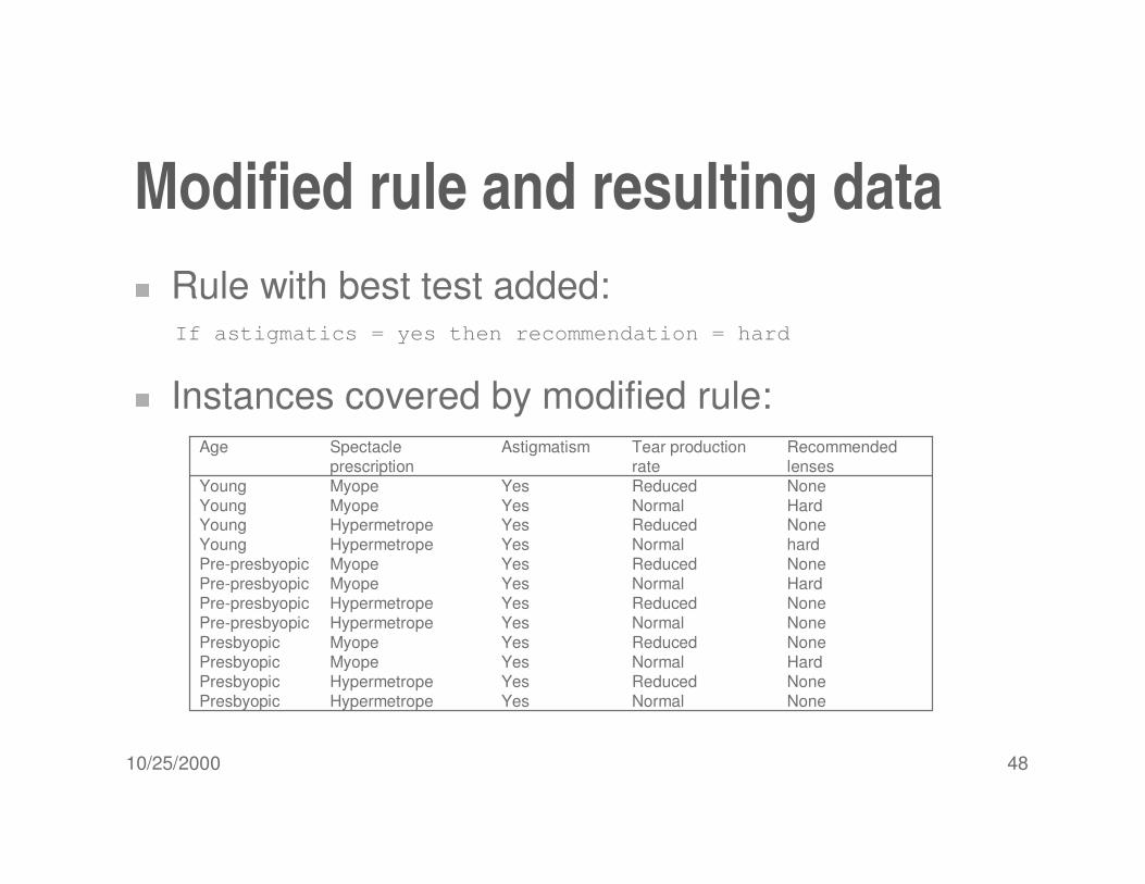
Modified rule and resulting data( Rule with best test added:

( Instances covered by modified rule:

If astigmatics = yes then recommendation = hard

NoneReducedYesHypermetropePre-presbyopic NoneNormalYesHypermetropePre-presbyopicNoneReducedYesMyopePresbyopicHardNormalYesMyopePresbyopicNoneReducedYesHypermetropePresbyopicNoneNormalYesHypermetropePresbyopic

HardNormalYesMyopePre-presbyopicNoneReducedYesMyopePre-presbyopichardNormalYesHypermetropeYoungNoneReducedYesHypermetropeYoungHardNormalYesMyopeYoungNoneReducedYesMyopeYoung

Recommended lenses

Tear production rate

AstigmatismSpectacle prescription

Age

10/25/2000 49

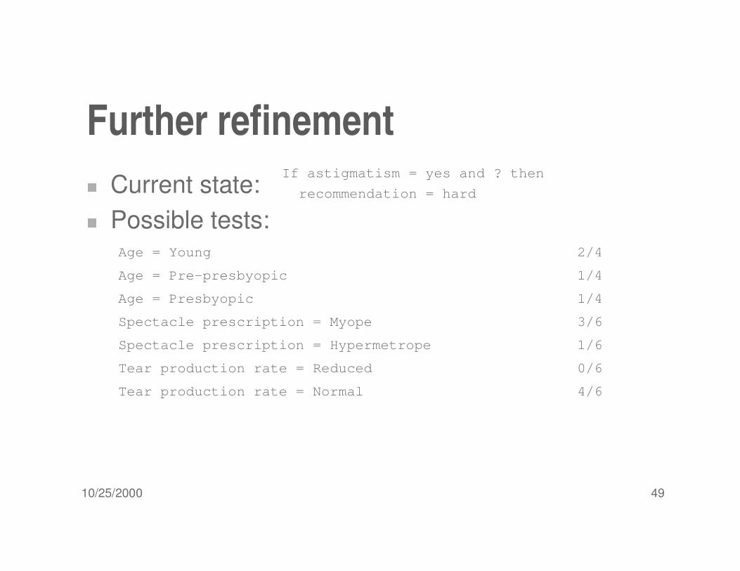
Further refinement) Current state:

) Possible tests:

4/6Tear production rate = Normal

0/6Tear production rate = Reduced

1/6Spectacle prescription = Hypermetrope

3/6Spectacle prescription = Myope

1/4Age = Presbyopic

1/4Age = Pre-presbyopic

2/4Age = Young

If astigmatism = yes and ? then

recommendation = hard

10/25/2000 50

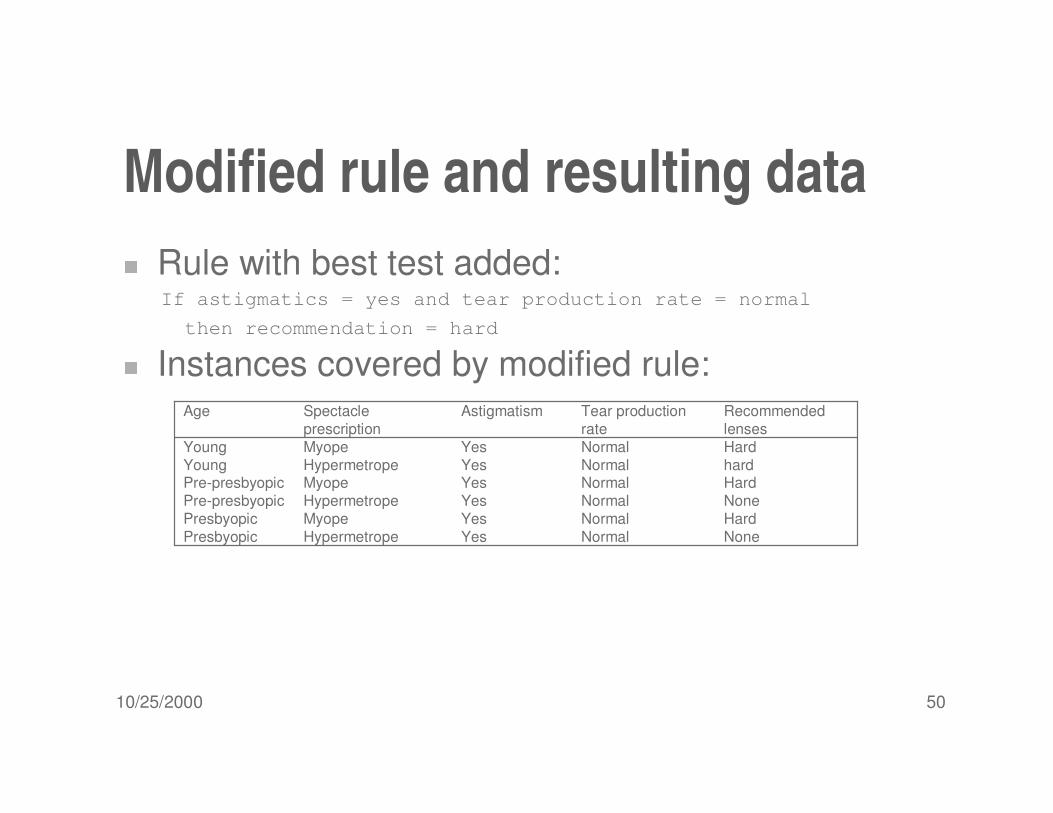
Modified rule and resulting data* Rule with best test added:

* Instances covered by modified rule:

If astigmatics = yes and tear production rate = normal

then recommendation = hard

NoneNormalYesHypermetropePre-presbyopicHardNormalYesMyopePresbyopicNoneNormalYesHypermetropePresbyopic

HardNormalYesMyopePre-presbyopichardNormalYesHypermetropeYoungHardNormalYesMyopeYoung

Recommended lenses

Tear production rate

AstigmatismSpectacle prescription

Age

10/25/2000 51

Further refinement+ Current state:

+ Possible tests:

+ Tie between the first and the fourth test

, We choose the one with greater coverage

1/3Spectacle prescription = Hypermetrope

3/3Spectacle prescription = Myope

1/2Age = Presbyopic

1/2Age = Pre-presbyopic

2/2Age = Young

If astigmatism = yes and

tear production rate = normal and ?

then recommendation = hard

10/25/2000 52

The result- Final rule:

- Second rule for recommending “hard lenses”:(built from instances not covered by first rule)

- These two rules cover all “hard lenses”:

. Process is repeated with other two classes

If astigmatism = yes and

tear production rate = normal and

spectacle prescription = myope

then recommendation = hard

If age = young and astigmatism = yes and

tear production rate = normal then recommendation = hard

10/25/2000 53

Pseudo-code for PRISMFor each class C

Initialize E to the instance set

While E contains instances in class C

Create a rule R with an empty left-hand side that predicts class C

Until R is perfect (or there are no more attributes to use) do

For each attribute A not mentioned in R, and each value v,

Consider adding the condition A = v to the left-hand side of R

Select A and v to maximize the accuracy p/t

(break ties by choosing the condition with the largest p)

Add A = v to R

Remove the instances covered by R from E

10/25/2000 54

Rules vs. decision lists/ PRISM with outer loop removed generates a

decision list for one class

0 Subsequent rules are designed for rules that are not covered by previous rules

0 But: order doesn’t matter because all rules predict the same class

/ Outer loop considers all classes separately

0 No order dependence implied

/ Problems: overlapping rules, default rule required

10/25/2000 55

Separate and conquer1 Methods like PRISM (for dealing with one class)

are separate-and-conquer algorithms:

2 First, a rule is identified

2 Then, all instances covered by the rule are separated out

2 Finally, the remaining instances are “conquered”

1 Difference to divide-and-conquer methods:

2 Subset covered by rule doesn’t need to be explored any further