inferring mechanical resonances in micro - and
TRANSCRIPT

Clemson UniversityTigerPrints
All Dissertations Dissertations
8-2008
INFERRING MECHANICAL RESONANCESIN MICRO - AND NANOCANTILEVERSUSING THE HARMONIC DETECTION OFRESONANCE (HDR) METHOD TODEVELOP A NOVEL SENSING PLATFORMGayatri KeskarClemson University, [email protected]
Follow this and additional works at: https://tigerprints.clemson.edu/all_dissertations
Part of the Materials Science and Engineering Commons
This Dissertation is brought to you for free and open access by the Dissertations at TigerPrints. It has been accepted for inclusion in All Dissertations byan authorized administrator of TigerPrints. For more information, please contact [email protected].
Recommended CitationKeskar, Gayatri, "INFERRING MECHANICAL RESONANCES IN MICRO - AND NANOCANTILEVERS USING THEHARMONIC DETECTION OF RESONANCE (HDR) METHOD TO DEVELOP A NOVEL SENSING PLATFORM" (2008).All Dissertations. 244.https://tigerprints.clemson.edu/all_dissertations/244
INFERRING MECHANICAL RESONANCES IN MICRO - AND NANOCANTILEVERS USING THE HARMONIC DETECTION OF RESONANCE
(HDR) METHOD TO DEVELOP A NOVEL SENSING PLATFORM
A Dissertation Presented to
the Graduate School of Clemson University
In Partial Fulfillment of the Requirements for the Degree
Doctor of Philosophy Materials Science and Engineering
by Gayatri Keskar August 2008
Accepted by: Dr. Apparao Rao, Committee Chair
Dr. John Ballato Dr. Jian Luo
Dr. Igor Luzinov

ABSTRACT
During the past two decades, advances in microelectromechanical systems
(MEMS) have spurred efforts worldwide to develop sensing platforms based on smart
microcantilevers. A microcantilever beam is one of the simplest MEMS structures which
forms the basis for portable, fast and highly sensitive schemes that are capable of
measuring small deflections in static or dynamic response due to changes in external
parameters such as mass, pressure, charge, etc.
In this dissertation, I mainly focus on MEMS sensors with transducers in the form
of microcantilevers. Variations in the microcantilever’s response such as resonant
frequency, amplitude, phase and quality factor when exposed to external stimuli are
measured. Recently, we have developed a fully electrical sensing platform called the
harmonic detection of resonance (HDR) method by which a silicon microcantilever (or a
multiwalled carbon nanotube) can be electrically actuated and its resonance parameters
electrically detected [4, 5] through capacitance changes. It is well known that a large
interfering signal coming from the inherent parasitic capacitance in the circuit at the
driving frequency Ω, is present in the platforms which use the capacitive readout method.
However, we found that by driving the cantilever at Ω and detecting its response at
higher harmonics of Ω, the parasitic capacitance can be avoided, facilitating the
measurement of dynamic capacitance with high sensitivity in micro and nano-cantilevers
[1, 2]. A significant part of this dissertation is devoted to the study of the nonlinear
dynamics of microcantilevers under varying gas environments and pressures using HDR
ii

[3]. I also discuss the characteristics of an electrostatically driven microcantilever which
exhibits Duffing-like behavior using HDR. The first experimental demonstration of its
potential use as a highly sensitive sensing platform is discussed. [4]. We also discuss the
behavior of an unfunctionalized microcantilever sensor which can be used for active
sensing of gaseous species under ambient conditions. Our sensing platform measures the
changes in the mechanical response (in amplitude and/or phase) of the vibrating
microcantilever in air at its resonant frequency when exposed to several vapors and gases
[5]. Finally I present the preliminary results on sensing toxic gases using functionalized
microcantilevers.
In the final chapter, I present evidence for the fact that HDR method is scaleable
and can be adapted for nanoscale cantilevers. In particular, I introduce the reader to
bending modulus measurements of multiwalled carbon nanotubes performed in Prof.
Rao’s group. One of the key factors in these measurements is an accurate knowledge of
density of carbon nanotubes. I provide in-depth discussion of the gradient sedimentation
technique which enables one to measure the density of both single- and multi-walled
carbon nanotubes.
iii

DEDICATION
I dedicate this work to my mother, Madhavi Keskar, father Deepak Keskar and to
my brother Hrishikesh Keskar. I take this opportunity to express my sincere gratitude
towards all my family for their unconditional love, good wishes and continuous support.
iv

ACKNOWLEDGMENTS
I would like to thank those who were instrumental in my development as a
scientist especially my advisor, Dr. Apparao Rao; Dr. Malcolm Skove; my labmate,
Bevan Elliott and my roommate Sonia Ramnani.
Dr. Apparao Rao, has given me his valuable guidance and wholehearted support
for all this time. My research has been inspiring and challenging with his constructive
criticism and words of encouragement in all aspects of my work. Besides being an
excellent advisor, he has been a fatherly figure to me. I am fortunate to have him as my
mentor in my life. I am very grateful to all other committee members: Dr. J. Ballato, Dr.
J. Luo and Dr. I. Luzinov for reviewing my dissertation.
Dr. Malcolm Skove has been actively involved in this project right from day one.
It was his knowledge of the electronics and the lock-in amplifiers that helped us develop
the HDR method. He has worked out the theory for HDR particularly for chapters 3 and
4. We have worked closely together in the lab for the last three years everyday learning
something new from him.
Bevan has always guided me in the right direction with his valuable inputs. In
addition to his contributions to this research, Bevan has become a great friend. He has
always inspired me to keep going and has always trusted that I would overcome each and
every challenge faced in graduate school and in life.
Sonia with whom I have a relationship like no one else, has always motivated me
with a positive energy and right spirit. I am very fortunate to have her everytime with me
v

to solve all my problems which mean a lot to me. To Sonia, without your unconditional
love and support, I would not have ever made it this far.
I would like to thank Jay Gaillard who has developed this HDR technique for
teaching me HDR which is the backbone of my work. I have spent the most important
period of my graduate school learning all about MEMS and NEMS from him. Some of
his results about measuring the resonance on nanoscale are explained briefly in chapter 6.
I would also like to thank Razvan for developing the mathematical model for determining
the density of carbon nanotubes along with the determination of Young’s modulus of a
Multiwall carbon nanotube used in chapter 6. I would like to acknowledge those in the
group with whom I have worked directly or indirectly and have spent time enjoying this
graduate experience like Rahul, Ted, Jason, J D, Rama and Yang.
I would like to thank Qi Lu and Dr. L. Larcom for their valuable contribution in
the gradient sedimentation study. I would like also to thank Joan and Amar at the AMRL
for their willingness to lend their expertise, time and effort which were necessary in the
completion of this dissertation. Special thanks to the staff of Department of Physics and
Astronomy and Materials Science and Engineering.
Last but not the least I give my deepest and most sincere gratitude to all my
friends for their friendship and support throughout my graduate career. Special thanks to
my close friends Malay, Gauri, Nikhil, Niten, Tanuja, Radhika, Shail and Sudeep for
making this whole journey towards my doctorate so memorable.
vi

TABLE OF CONTENTS
Page
TITLE PAGE....................................................................................................................i ABSTRACT.....................................................................................................................ii DEDICATION................................................................................................................iv ACKNOWLEDGMENTS ...............................................................................................v LIST OF TABLES..........................................................................................................ix LIST OF FIGURES .........................................................................................................x CHAPTER I. INTRODUCTION .........................................................................................1 Introduction..............................................................................................1 History of microcantilever based sensors ................................................2 Resonance response .................................................................................3 Sensing techniques...................................................................................4 Sensor applications ..................................................................................6 II. GENERAL THEORY..................................................................................10 Actuation methods .................................................................................10 Detection methods .................................................................................12 Theory of cantilevered beams................................................................20 III. USING ELECTRIC ACTUATION AND DETECTION OF OSCILLATIONS IN MICROCANTILEVERS FOR PRESSURE MEASUREMENTS ...........................................28 Introduction............................................................................................28 Harmonic Detection of Resonance (HDR) ............................................29 Quality factor (QE) .................................................................................33 Resonant frequency and spring softening ..............................................36 Experiment.............................................................................................37 Results and discussion ...........................................................................38 Conclusions............................................................................................54
vii
Table of Contents (Continued)
Page
IV. ULTRA-SENSITIVE DUFFING BEHAVIOR OF A MICROCANTILEVER ........................................................................56 Introduction............................................................................................56 Mathematical model...............................................................................58 Duffing mechanism................................................................................62 Experimental setup.................................................................................64 Results and discussion ...........................................................................64 Summary ................................................................................................85 V. ACTIVE SENSING IN AMBIENT CONDITIONS USING AN ELECTROSTATICALLY DRIVEN SILICON MICROCANTILEVER...................................................87 Introduction............................................................................................87 Experimental Details..............................................................................89 Results and discussion ...........................................................................91 Conclusions..........................................................................................116 VI. DETERMINATION OF CARBON NANOTUBE DENSITY BY GRADIENT SEDIMENTATION…….......................119 Introduction..........................................................................................119 Experimental procedure .......................................................................121 Results and discussion .........................................................................122 Measuring resonance in a nanocantilever (MWNT) using HDR.........136 Conclusions..........................................................................................140 APPENDICES .............................................................................................................142 A: Procedure for making sensor chip..............................................................143 B: Procedure for etching tungsten probe tips .................................................145 C: Operating principle of Mass flow controllers ............................................147 D: Equipment list ............................................................................................149 REFERENCES ............................................................................................................150
viii

LIST OF TABLES
Table Page 2.1 Solution of the equation of motion for a cantilever beam ...........................25 4.1 Summarizing Duffing behavior under various experimental conditions .........................................................................68 6.1 The measured densities of various structures of CNTs. ............................125 6.2 Measured and Computed Densities of MWNTs compared with those reported in the literature. ....................................................136
ix
LIST OF FIGURES
Figure Page
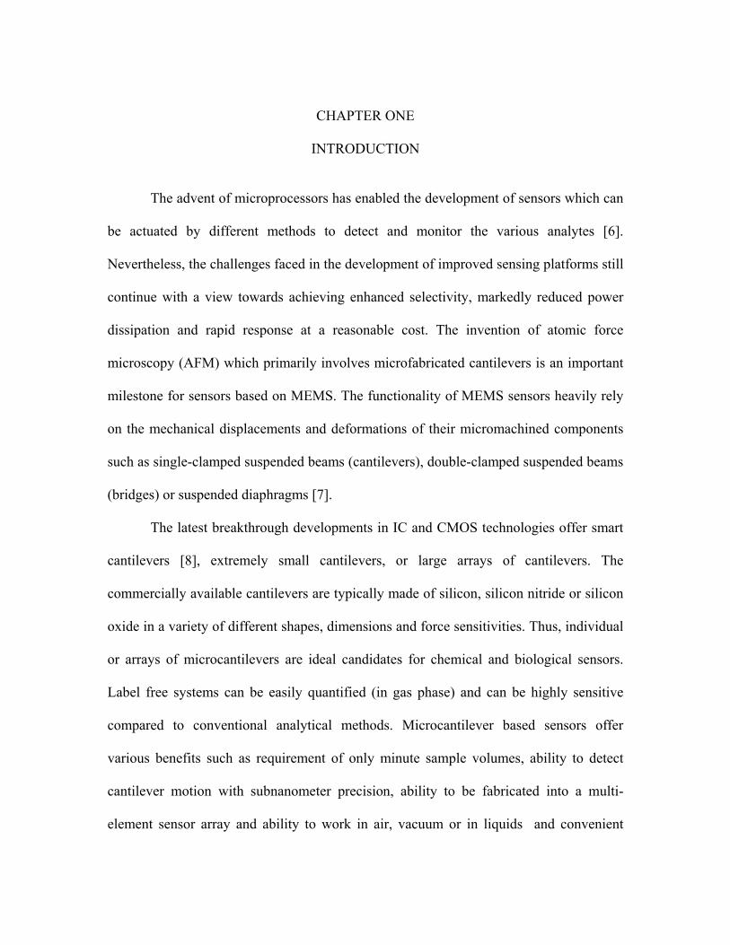
1.1 Various transduction mechanisms implemented by cantilever transducers to convert input stimuli into output signals .....................................................................................5
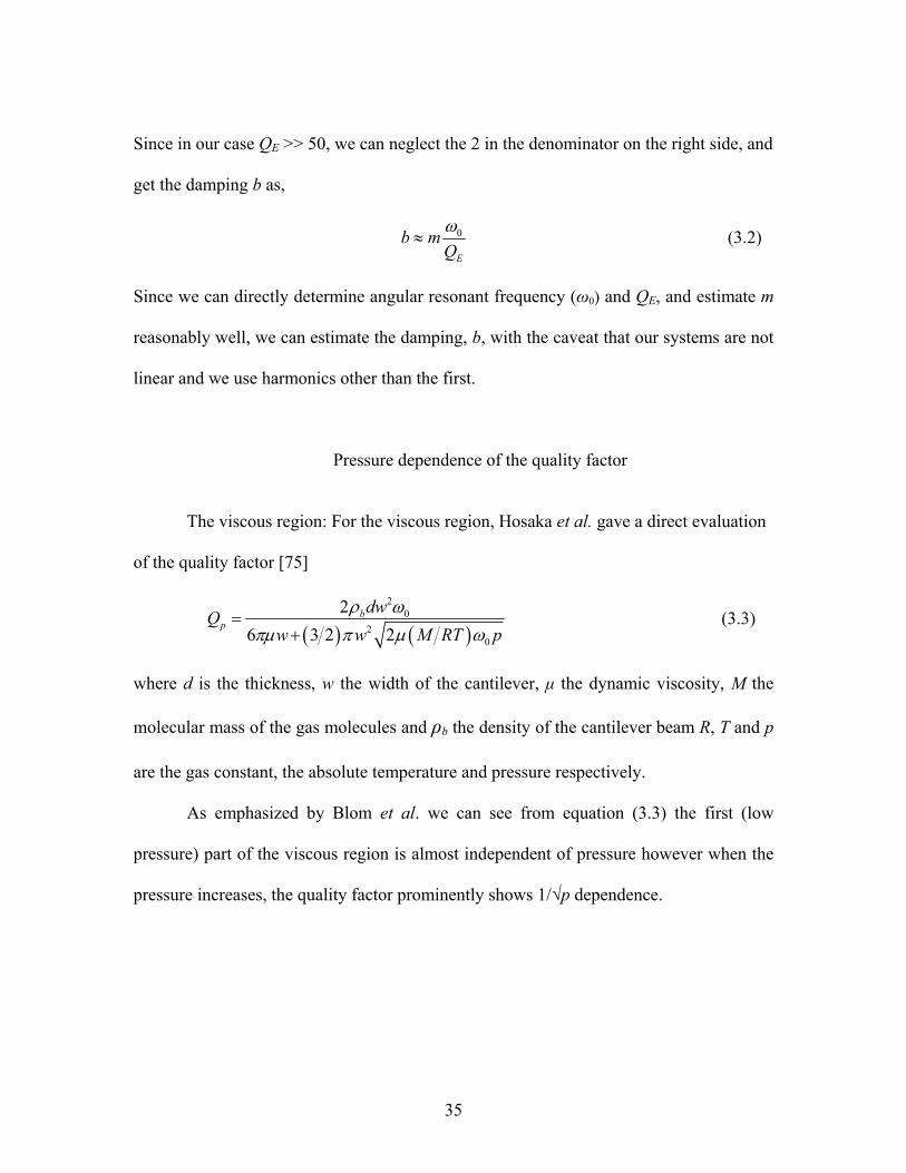
1.2 Summary of the wide spectrum of applications that can be realized using micro-cantilevers...................................................8 2.1 Schematic illustration of electrostatic actuation ..........................................12 2.2 The optical detection scheme commonly used to measure deflections of microfabricated cantilever probes in AFM .....................14 2.3 Measuring resonance of individual carbon nanotubes by in situ TEM. .....................................................................................15 2.4 (a) Piezoresistive cantilever which can be used for AFM as well as MEMS senors, (b): Optical image of a piezoelectric (ZnO) multimorph ....................................17 2.5 Capacitive readout technique commonly used for electrically excited cantilevers...............................................................18 2.6 Flexural behavior of a straight beam and its stress distribution .............................................................................................21 3.1 A schematic of the experimental set up using our harmonic detection of resonance method for sensing pressure changes. ................................................................31 3.2 Amplitude (bullets) and phase (crosses) of the cantilever near the resonance frequency for 760 (blue) and 3E-3 torr (red) when measured at the 2nd harmonic (Vdc = 9 V, Vac = 5 V) with 8 μm gap distance..........................................................................41 3.3 (a) Resonance spectra of the 2nd harmonic at different pressures in air ......................................................................................42
x

List of Figures (Continued) Figure Page 3.3 (b) Resonance spectra at the 2nd harmonic at different pressures in a helium environment.. ......................................................43 3.4 1/QE as a function of pressure......................................................................44 3.5 (a) Comparison of the experimental results (shown by red squares, left hand axis) for QE as a function of pressure using HDR (red squares) and Q as measured by Bianco et al. (shown by blue circles, right hand axis) using piezoelectric excitation and optical detection. ..................................45 3.5 (b) Our experimental results (shown by red squares, left hand axis) for the normalized variation of resonant frequency as a function of pressure using HDR and the experimental data presented by Bianco et al. (shown by blue circles, right hand axis) in the viscous region. .........................................................46 3.6 (a) Dependence of QE on the molecular mass of the surrounding gas measured at the 2nd harmonic at ambient pressure with Vdc = 9 V, Vac = 10 V at 12 μm gap distance. ...............................................................47 3.6 (b) Resonance frequency spectra under different gas environments at the 2nd harmonic at ambient pressure with Vdc = 9 V, Vac = 10 V. ..............................................................48 3.7 (a) Amplitude response to chamber pressure at the 2nd harmonic. The inset shows the dependence of QE on the pressure at the 2nd harmonic at Vdc = 9 V, Vac = 4.4 V. ................................................................................51 3.7 (b) Amplitude response to chamber pressure at the 3rd harmonic. The inset shows the dependence of QE on the pressure at the 3rd harmonic at (Vdc = 9 V, Vac = 6.2 V) ...............................................................................52
xi

List of Figures (Continued) Figure Page 3.8 (a) Comparison of the resonant frequency of the cantilever as a function of pressure at the 2nd (Vdc = 9 V, Vac = 4.4 V) and 3rd (Vdc = 9 V, Vac = 6.2 V) harmonics in a He environment ............................53 3.8 (b) Comparison of amplitudes at f0 of the cantilever as a function of pressure at the 2nd (Vdc = 9 V, Vac = 4.4 V) and 3rd (Vdc = 9 V, Vac = 6.2 V) harmonics in a He environment. ................................................54 4.1 Cartoon of steady state solutions under different excitation amplitudes showing three stages of Duffing behavior...........................63 4.2 (a) Frequency spectra under vacuum. Dark circles are used for increasing and light circles for decreasing f............................66 4.2 (b) Data at 2 Vac from Fig. 4.2(a) in a polar plot in which the angle is the phase and the radius is the amplitude of the response with increasing (dark circles) and decreasing (light circles), f as a parameter.................................67 4.2 (c) Data at 3 Vac from Fig. 4.2(a) in a similar polar plot..............................68 4.2 (d) Data corresponding to Fig. 3.7 (b) in polar plot under vacuum at 3rd harmonic (Vdc = 9 V, Vac = 6.2 V)...................................69 4.3 Measured frequency spectra under vacuum (5 torr) with increasing and decreasing f ...........................................................71 4.4 Measured frequency spectra under 760 torr of hydrogen with increasing and decreasing f ...........................................................72 4.5 Measured frequency spectra in air at 3rd harmonic with 8 μm gap distance with increasing and decreasing f ................................73 4.6 Measured frequency spectra in air at 4th harmonic with 8 μm gap distance with increasing and decreasing f ................................75 4.7 Measured frequency spectra in air at 5th harmonic with 8 μm gap distance with increasing and decreasing f. ...............................76
xii

List of Figures (Continued) Figure Page 4.8 Measured frequency spectra in air at 6th harmonic with 8 μm gap distance with increasing and decreasing f. ...............................77 4.9 Measured frequency spectra in air at 3rd harmonic with 4 μm gap distance with increasing and decreasing f ................................79 4.10 Measured frequency spectra in air at 4th harmonic with 4 μm gap distance with increasing and decreasing f ................................80 4.11 Measured frequency spectra in air at 5th harmonic with 4 μm gap distance with increasing and decreasing f showing ON / OFF characteristics...................................................81 4.12 Measured frequency spectra in air at 6th harmonic with 4 μm gap distance with increasing and decreasing f ................................82 4.13 Measured frequency spectra in air with increasing and decreasing f at all the harmonics with an 8 μm gap distance (Vac = 9.75 V, Vdc = 9.6 V).................................................83 4.14 Sensing a pressure change from 5×10⁻⁵ torr to 7×10⁻⁵ torr using the Duffing behavior at the 2nd harmonic in the backward direction at 8 μm gap distance (Vac = 1.3 V, Vdc = 4 V)..............................................................85 5.1 (a) Schematic diagram of the HDR system modified for sensing gases and solvents .....................................................................90 5.1 (b) Digital photograph of the experimental set up illustrating the chip carrier with cantilever and counter electrode and other electronic connections. The inset shows the optical image of cantilever – counter electrode alignment.................................................91 5.2 (a) Response spectrum showing amplitude (solid red squares) and phase (solid blue circles) upon exposure to 100 sccm of air continuously bubbled through methanol ......................................................................93
xiii

List of Figures (Continued) Figure Page 5.2 (b) Response of the cantilever at the selected f0 = 17.69 kHz showing the ΔA (solid red squares) and ΔΦ (solid blue circles) upon exposure to puffs of 100 sccm of air bubbled through methanol..........................94 5.3 (a) Response spectrum showing amplitude (solid red squares) and phase (solid blue circles) upon exposure to 100 sccm of methane (CH4).........................................................96 5.3 (b) Response of the cantilever vibration to puffs of methane (CH4) when the selected f0 is 17.71 kHz, showing ΔA (solid red squares) and ΔΦ (solid blue circles) upon exposure to 30 sec puffs of 100 sccm of methane (CH4)........................................................97 5.4 (a) Response spectrum showing amplitude (solid red squares) and phase (solid blue circles) upon exposure to 100 sccm of nitrous oxide (N2O) ....................................................98 5.4 (b) Response at f0 = 17.7 kHz, showing ΔA (solid red squares) and ΔΦ (solid blue circles) upon exposure to 100 sccm puffs of nitrous oxide (N2O)........................................99 5.5 (a) Response spectrum showing amplitude (solid red squares) and phase (solid blue circles) upon exposure to 100 sccm of protium (H2)...........................................100 5.5 (b) ΔA (solid red squares) and ΔΦ (solid blue circles) upon exposure to puffs of 100 sccm of protium (H2) at 17.71 kHz...................................................................................101 5.5 (c) Response spectrum showing amplitude (solid red squares) and phase (solid blue circles) upon exposure to 100 sccm of deuterium (D2).......................................................102 5.5 (d) Response of ΔA (solid red squares) and ΔΦ (solid blue circles) upon exposure to 100 sccm of deuterium (D2) when the selected f0 = 17.71 kHz. ..........................................103
xiv

List of Figures (Continued) Figure Page 5.5 (e) In a second experiment, ΔA upon exposure to puffs of 100 sccm of deuterium (D2) (solid red squares) and protium (H2) (red crosses) at 17.6 kHz. ..................................104 5.6 Dependence of ΔΑ and ΔΦ (measured at the selected f0 = 17.71 kHz) on the amount concentration of protium (H2) molecules present in the vicinity of the cantilever. The inset shows the response spectra upon exposure to puffs of increasing concentration of protium from 50 to 800 sccm..................106 5.7 (a) Normalized amplitude changes upon exposure of the cantilever vibrating near f0 to 100 sccm of air bubbled through water, iso-propanol, methanol, benzene and n-hexane ..............................................................109 5.7 (b) The normalized amplitude ∆A/A for the solvents methanol, water, iso-propanol, benzene and n-hexane plotted as a function of three normalized parameters: the inverse of mass, dielectric constant and polarity index. ..........................................................................110 5.8 Dependence of normalized amplitude on the molecular mass of the gas surrounding the cantilever upon exposure to 100 sccm of protium, deuterium, methane and nitrous oxide. ......................................................111 5.9 (a) Response spectra comparing amplitudes upon exposure to 100 sccm of hydrogen bubbled through different flavors such as grape water, orange juice, Diet Coca Cola™, regular Coca Cola™, Cherry Coca Cola Zero™ and apple juice .....................................112 5.9 (b) Response spectra comparing phases upon exposure to 100 sccm of hydrogen bubbled through different flavors such as grape water, orange juice, Diet Coca Cola™, regular Coca Cola™, Cherry Coca Cola Zero™ and apple juice .....................................113
xv

List of Figures (Continued) Figure Page 5.10 (a) Resonance spectra showing upshift in the resonant frequency (blue) after functionalizing the cantilever with 11-MUA.................................................................................115 5.10 (b) Three separate measurements showing the change in amplitude when exposed to 400 ppm of ammonia in helium (solid blue circles).The amplitude in pure He is shown in solid red circles ................................................................................116 5.11 The ΔA signal increases monotonically with the increase in the concentration of hydrogen sulphide gas in helium from 0 to 100 ppm in the chamber.....................................117 6.1 Various structures of CNTs, including (a) acid-SWNT, (b) p-SWNT, (c) MWNT and (d) iso-SWNT, form bands at different levels in gradients prepared and run identically....................................................................124 6.2 Raman characterization of MWNTs, p-SWNTs and iso- SWNTs. The two peaks in the spectrum of iso- SWNTs marked by “Si” were from silicon substrate ...................125 6.3 The density profile along the length of a gradient obtained from p-SWNTs......................................................................126 6.4 TEM images obtained from (a) SWNTs, (b) SWNT bundles and (c) MWNTs......................................................................128 6.5 (a) The density of SWNT bundles was computed based on the arrangement of SWNTs in tiers. ...............................................130 6.5 (b) The density of SWNTs plotted as a function of the diameter of bundles. Both computational (crosses, open triangles, and open circle) and experimental (solid square, solid triangle, and solid diamond) densities are presented .......................................134
xvi
xvii
List of Figures (Continued) Figure Page 6.5 (c) Illustration of MWNT based on continuum hypothesis. The multi-shells are treated as continuum medium with thickness h and length L.................................................................135 6.6 The amplitude (solid circles) and phase (open circles) spectra of a MWNT (7 µm long and 50 nm in diameter) near resonance measured under ambient conditions. The inset shows an optical dark field image of the MWNT placed parallel to the W tip (counter electrode) with 5 µm scale bar . .............................137 6.7 (a) Dark field microscope image of the geometrical setup for the MWNT and the counter electrode assembly ............................138 6.7 (b) A schematic of mechanical oscillations induced in a MWNT by the force (FC), when the MWNT and the counter electrode are separated by a distance (s)...........................138 6.7 (c) The amplitude (light circles) and phase (light triangles) spectra near the resonance of MWNT. The amplitude (dark circles) and phase (dark triangles) signals obtained for the same geometry of W probe tip in the absence of MWNT..................................................139
CHAPTER ONE
INTRODUCTION
The advent of microprocessors has enabled the development of sensors which can
be actuated by different methods to detect and monitor the various analytes [6].
Nevertheless, the challenges faced in the development of improved sensing platforms still
continue with a view towards achieving enhanced selectivity, markedly reduced power
dissipation and rapid response at a reasonable cost. The invention of atomic force
microscopy (AFM) which primarily involves microfabricated cantilevers is an important
milestone for sensors based on MEMS. The functionality of MEMS sensors heavily rely
on the mechanical displacements and deformations of their micromachined components
such as single-clamped suspended beams (cantilevers), double-clamped suspended beams
(bridges) or suspended diaphragms [7].
The latest breakthrough developments in IC and CMOS technologies offer smart
cantilevers [8], extremely small cantilevers, or large arrays of cantilevers. The
commercially available cantilevers are typically made of silicon, silicon nitride or silicon
oxide in a variety of different shapes, dimensions and force sensitivities. Thus, individual
or arrays of microcantilevers are ideal candidates for chemical and biological sensors.
Label free systems can be easily quantified (in gas phase) and can be highly sensitive
compared to conventional analytical methods. Microcantilever based sensors offer
various benefits such as requirement of only minute sample volumes, ability to detect
cantilever motion with subnanometer precision, ability to be fabricated into a multi-
element sensor array and ability to work in air, vacuum or in liquids and convenient

parallelization because of batch silicon micro-machining techniques [9]. The
microcantilevers can be heated and cooled with a thermal time-constant less than a
millisecond due to their low thermal mass. This is beneficial for regenerating the sensor
through rapid reversal of molecular absorption processes which is essential for in situ
sensing platforms [10].
History of microcantilever based sensors
These miniaturized devices perform based on the underlying principle of
mechanical stress and deformations induced due to variations in the surrounding
environment. Since the 1920s, macroscopic cantilever devices and mechanical resonators
were well established for measuring the mechanical responses to adsorbate-induced
stresses using optical means in chemical and biological sensors. But, macroscale
mechanical transducers could hardly satisfy the demand for highly specific sensing
performance because of extremely high susceptibility to external vibrations stemming
from large suspended masses and relatively low resonance frequencies and thus 1/f noise.
Hence, these transducers failed to achieve practical importance until microcantilevers and
more precise detection schemes were widely available enabling from a macro to micro-
mechanical transition [7].
2

Resonance Response
Depending on the measured parameter i.e. either cantilever deflection or
resonance frequency, the mode of cantilever operation can be referred to as (1) static: for
example, functionalizing one side of the cantilever with a sensing layer so that the
cantilever bends due to the surface stress due to a specific reaction between the analyte
and the sensing layer [3] or (2) dynamic: detects the shift in resonant frequency of the
cantilever due to specific mass adsorption (Fig. 1.1) [11]
Static cantilever deflections may arise from either external forces acting on the
cantilever or intrinsic stresses generated within or on the cantilever surface. These
intrinsic stresses may be result from thermal expansion, interfacial processes or
physicochemical variations of the cantilever. In the dynamic mode, the resonant
frequency essentially varies with the adsorbed mass and viscoelastic properties of the
medium around the cantilever. The broad range of transduction modes stems from the
fact that a stimulus of each type may affect the cantilever directly or may undergo several
transformations before affecting the mechanical parameters of the cantilever under study.
The transduction efficiency of the static mode increases with the reduction of the stiffness
of the cantilever. Hence, longer cantilevers with small spring constant are suitable for the
operation in the static (adsorption-bending) mode. Whereas shorter, higher resonant
frequency cantilevers are ideal for the frequency shift based approach The sensitivity of
the resonant mode increases with the operation frequency[12].
3

Sensing Techniques
Microcantilever sensors can be physical, chemical, or biological sensors
depending upon the nature of the input stimuli. The shift in the resonant frequency can be
used as an indicator to detect any change in the surrounding environment that affects the
mass, elasticity or damping of the microcantilever. Applications as sensitive physical
sensors include detection of the changes in the physical parameters such as viscosity,
pressure, density, and flow rate [13]. The detection limit of the microcantilever based
physical sensors is ~ 1 pN for measuring forces and for displacement measurements, 0.1
nm. The viscosity of gases and liquids can also be determined using the resonance
response of a microcantilever [14].
Using microcantilever based biosensors, the detection of protein adsorption,
antibody-antigen recognition, and DNA hybridization has been successfully
demonstrated [15, 16] as they can be operated in liquid. However, the liquid medium
damps the resonance response of a microcantilever to approx. one order of magnitude
smaller than while operating in air [17-19]. Thus the main problem is the high damping
and not the biological preparation for the microcantilever based biosensors.
4
Figure 1.1 Various transduction mechanisms implemented by cantilever transducers to
convert input stimuli into output signals [7].
A chemical sensor comprised of a physical transducer and a chemically selective
layer produces output signals as a response to the chemical stimuli. The affinity of the
targeted analytes for the specific binding sites in the highly selective receptor layers helps
in the recognition of various molecules. There can be two types of gas- solid interactions:
bulk-like absorption and surface- like adsorption [20]. In general, adsorption decreases
the surface energy. The extent of cantilever deflection depends directly on the changes in
the surface energy due to molecular adsorption. This in turn varies with the deviation in
free energy per adsorbate and the total number of molecules involved in the adsorption
process.
5

The adsorption-induced forces are large enough to rearrange the lattice locations
of the surface and subsurface atoms on a clean surface, causing surface relaxations and
reconstructions. Molecular adsorption on a cantilever coated on only one side causes
bending because of adsorption induced changes in the surface stress [10, 21, 22].
Whereas for the cantilever with two differently coated chemical surfaces, molecular
adsorption results in a differential stress between the top and bottom surfaces of the
cantilever leading to it’s bending.
The ability to functionalize one surface of the silicon microcantilever so that a
given molecular species will be preferentially bound to that surface upon exposure to a
vapor stream vastly enhances the selectivity of the detection. Thus functionalized
microcantilevers enable the sensor to perform as chemical/artificial nose [9]. Analyte
detection using miniaturized chemical sensors has various applications in different fields
such as quality and process control, biomedical analysis, gas-sensing devices, forensic
investigations, fragrance design and oenology [23].
Sensor Applications
1) Mass sensor - A microcantilever can be used as a microbalance with
femtogram mass resolution [9] by measuring the shifts in the resonant frequency. For
mass sensitive gas sensors, the sensors response depends on the mass of an absorbed
analyte which in turn depends on the concentration of the analyte and its molecular
weight. Mass sensitive transducers are the active devices and are commonly classified as
Bulk Acoustic Wave (BAW) and Surface Acoustic Wave (SAW) sensors. These
6
transducers are piezoelectrically excited in which the resonance frequency is a measure of
the mass of the transducer, and is affected by the analyte concentration to be determined
[24].
2) Temperature sensor - Berger et al. [25] and Thundat et al. [13, 26] pioneered
cantilever based sensors and their work involved the measurements nanoscale deflections
due to an external stimuli. The bending along with the static deflections of the cantilever
has been attributed to the surface stress changes involving heat transfer from chemical
reactions or phase transitions.
3) Optical sensors - Thundat et al. [27] also demonstrated the detection of
ultraviolet radiation at pJ levels based on the microcantilevers coated with UV- sensitive
polymers. The cross-linking of a polymer due to UV- radiation exposure results in a
change in the cantilever resonant frequency and the spring constant.
4) Magnetic sensors – Many research groups have reported the measurements of
the magnetic properties of magnetic and superconducting materials using a
microcantilever [28-30]. Using the torque induced by an applied field, Rossel et al [28]
studied the magnetization of small (< microgram) samples mounted at the ends of a
cantilever with peizoresistive read-out (discussed in next chapter). Such cantilevers are
capable of sensing torques that are approx. 10-14 Nm. In case of an applied field of 1T,
magnetic moments as small as approx. 10-14Am2 can be measured with microcantilevers,
which is 3 orders of magnitude greater than the commercial SQUID (superconducting
quantum interference device) magnetometers.
7
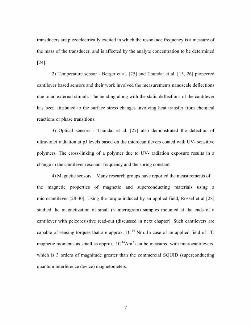
Figure 1.2: Summary of the wide spectrum of applications that can be realized using
micro-cantilevers [23].
Figure 1.2 summarizes some of the techniques which have evolved from a
scanning force microscope (SFM) which uses a smart cantilever. A cantilever with an
integrated sharp tip can be used to study the surface profile of a sample as shown in Fig.
1.2(a) [31]. A one side metal-coated cantilever is useful as a micron scale temperature
sensor in which the bending is induced by the temperature change around the
microcantilever. The small thermal mass of the cantilevers enables very small heat
energy (~ nJ) to be measured and accurate changes in temperature have been measured
8

with a resolution of ≈10 μK (Fig. 1.2(b)). Detection of exothermic and endothermic phase
transitions involving ng amounts of material attached to the cantilever is feasible [32] (
Fig. 1.2(c)). Photothermal spectroscopy performed on the biomaterial cantilevers can be
used to measure the heat produced upon light irradiation, Fig. 1.2.(d) [33]. Fig. 1.2(e)
[34] describes the reaction of hydrogen and oxygen forming a water molecule catalyzed
by a platinum coated biomaterial cantilever using the oscillatory behavior (the figure
indicates the bending). Gold-thiol chemistry has been reported to self assemble a
monolayer of akylthiols on a gold coated cantilever. This in turn causes a change in the
surface stress which (as seen in Fig. 1.2(f)) [35] increases with increasing the chain
length of the alkylthiols. The change in mass due to gain or loss in the mass of the sample
attached to the apex of a cantilever can be measured by determining the shift in the
resonant frequency. The mass change that can be detected is in the range of 1 pg, Fig.
1.2(g). The change in the resonant frequency of a functionalized cantilever can be used to
monitor the variation in the environmental conditions (such as change in humidity based
on temperature). For thermogravimetric applications, the change in the mass of a sample
can be monitored as a function of the temperature by mounting a sample on the apex of
the vibrating cantilever, Fig 1.2(i) [36]. Using a cantilever deflection scheme, the various
forces such as electrostatic forces Fig. 1.2(j), or magnetic forces Fig. 1.2(k), can also be
detected.
9

CHAPTER TWO
GENERAL THEORY
Actuation Methods
Microcantilever based sensors often measure shifts in the resonant frequency. The
cantilever can be driven by just the thermal noise kBT in the absence of external actuation,
where kB is the Boltzman constant and T is the temperature [10]. However, at room
temperature the thermal energy is small and dependent on the environment in which the
cantilever resonates. Hence, cantilevers are often driven externally using common
actuation techniques for reliable use in many applications. The common actuation
techniques implemented to drive the microcantilevers externally are discussed here,
Piezoelectric actuation
The most commonly used actuation method to drive the cantilever is a
piezoelectric device. They are used extensively with AFM microcantilevers.
Commercially available scanning probe microscopes actuate the cantilevers by an
externally driving a piezoelectric device mounted close to the cantilever [38]. This
method utilizes certain crystalline materials, such as PbZrTiO3, which expand and
contract upon application of an electric field. For the AFM, a piezoelectric sheet is
sandwiched between two metal plates. One sheet is attached to the frame of the AFM. A
small (~3mm × 5mm rectangle) chip is placed on the other and the cantilever attached to
the chip. The frequency of the applied voltage is swept to provide a spectrum of the
10

response of the cantilever. From this spectrum, the fundamental resonant frequency of
the cantilever can be determined. The resonance induced with this method has limitations
while operating in liquid.
Magnetic actuation
Magnetic forces can be used for the actuation of the cantilever. These forces can
be induced by evaporating a magnetic layer on the cantilever or placing a magnetic
particle at the end of the cantilever and applying an external magnetic field by using a
solenoid. This method of actuation is used for AFM cantilevers in the tapping mode
while operating in liquids and for biological samples [37-41].
Electrostatic actuation
Among all the possible actuation techniques, electrostatic actuation is the most
preferred method in MEMS and nanoelectromechanical systems NEMS [42-44]. It is
convenient to incorporate this technique while fabricating microcantilever based systems.
A parallel plate configuration is implemented between the counter electrode and the
cantilever in order to vibrate the latter at its resonance. The basic principle here is to
determine the resonant frequency of the cantilever by sweeping the frequency of the ac
voltage. As can be seen in Fig. 2.1, an ac and a dc voltage are applied to counter
electrode, while the other plate which is a cantilever is connected to ground. The time
dependent force drives the motion of the cantilever, and when its frequency matches a
11

resonance of the cantilever, the amplitude of oscillating cantilever attains a maximum
value.
Figure 2.1: Schematic illustration of electrostatic actuation. The ac voltage along with dc
offset is applied to the counter electrode. The cantilever is grounded to maintain a
potential difference. The cantilever is driven into resonance by sweeping the frequency of
ac voltage.
Detection methods
The vital part of any cantilever based sensor is its deflection detection scheme
from which the changes in a specific parameter (directly related to its deflection in real
time) can be determined, often with at least nanometer accuracy [7]. In general, the
amplitude and the phase with respect to the driving force of a Fourier component of the
motion of the cantilever are measured as a function of the driving frequency. The
detection schemes are broadly classified as optical and electrical. While the optical beam
12

deflection technique is efficient and widely used in devices involving microcantilevers, it
is ineffective in the emerging technologies which involve the use of nanocantilevers. This
is due to the fact that nanocantilevers cannot reflect sufficient light for accurate
photodetection of a change in the deflection. This has led to the exploration of new
detection methods which can not only measure deflection in nanoscale cantilevers, but
can also be incorporated with MEMS and NEMS.
Optical method
The most commonly implemented detection scheme in modern AFM for
measuring cantilever deflections are optical beam deflection and optical interferometry
[45, 46]. The laser beam is focused near the free end of the cantilever which reflects it
onto a split photo diode or position - sensitive detector (Fig. 2.2). The reflected light
moves on the photodetector surface corresponding to the bending of cantilever. Two
pieces of the detector are measured in opposition, giving a null signal when the beam is
centered, and a large signal as the beam moves away from the center position. Using this
signal, cantilever displacements up to 10-14 m can be measured. This detection scheme is
very beneficial due to its linear response, simplicity, reliability, and need of no electric
connections to the cantilever.
13

Figure 2.2: The optical detection scheme commonly used to measure deflections of
microfabricated cantilever probes in AFM [7].
Visual detection
“Visual” detection is typically used for detecting the resonance in micro and
nanocantilevers including nanofabricated silicon cantilevers as well as cantilevered
nanotubes, nanowires, and nanobelts (Fig. 2.3). The various visual detection tools such as
transmission electron microscope [47], scanning electron microscope [48], field emission
microscope [49], or an optical microscope [50] can be used to measure electrically
induced mechanical oscillations in such cantilevers. However, the requirement of
14

portable sensing device for the measurements of environmental changes, such as
pressure, temperature, or presence of impurities limits its application.
Figure 2.3: Measuring resonance of individual carbon nanotubes by in situ TEM [51]. A
carbon nanotube which is (a) initially at its equilibrium position is electrically actuated to
resonate at its (b) first mode frequency (f1 = 1.21 MHz) and (c) at the second mode
frequency (f2 = 5.06 MHz).
15

Electrical Detection
The commonly used electrical detection techniques are the piezoresistance,
piezoelectric and capacitance detection [7].
1) Piezoresistance method: It is a phenomenon which results in a change in the crystal’s
electrical conductivity when the crystal is stressed. This method can be readily
implemented to monitor the stress induced in a cantilever, and therefore its deflection
from its equilibrium position. Stress sensors can be integrated on a chip containing a
cantilever and a Wheatstone bridge to measure the resisitivity. When a doped silicon
cantilever [52, 53] is deformed, it leads to a change in its resistance. Piezoresistive
cantilevers are designed with two identical legs in order to measure the resistance by
making electric connections to the two legs (Fig. 2.4 (a)). It is advantageous as compared
to the standard optical techniques as it involves no bulky and expensive optical
components. In addition it has ease of integrating it on the same chip using CMOs
technology without dealing with the tedious optical alignment. The main problem of this
technique is the current flow through the cantilever resulting in heating up of cantilever
and subsequent thermal shifts. It is ineffective in conducting liquids. The cantilevers
must have a double structure, which gets difficult to form on the nanoscale.
2) Piezoelectric method: The deposition of piezoelectric material, such as ZnO (Fig. 2.14
(b)), is necessary on the cantilever for this technique. During this effect, the deformation
of the cantilever induces the transient charges in the piezoelectric layer [54, 55]. One of
the drawbacks of this technique is the thickness of the piezoelectric layer is required to be
well above the optimal one in order to obtain large output.
16

The main disadvantage limiting the application of both piezoelectric and
piezoresistive methods in MEMS sensors is the need of electric connections to the
cantilever.
(a)
(b)
Figure 2.4 (a): Piezoresistive cantilever which can be used for AFM as well as MEMS
senors [7], (b): Optical image of a piezoelectric (ZnO) multimorph [55].
17

Capacitance method
The most promising capacitance readout method is based on measuring the
capacitance between two parallel conductor plates, where one is the cantilever and the
other is the fixed conductor on the substrate separated by a small gap [56]. The fixed
conductor is driven by applying an ac voltage with a dc offset and its frequency is swept
till it matches with the resonant frequency of the cantilever.
Figure 2.5: Capacitive readout technique commonly used for electrically excited
cantilevers[57].
Since, the capacitance is inversely proportional to the gap distance (s), the
sensitivity of this technique depends upon very small gap distance between the cantilever
18

and the substrate. The deformation of the cantilever causes the gap distance to change
which in turn changes the capacitance between the two conductor plates. The main
advantage of this method is that it can be easily integrated into MEMS and NEMS
devices which are fully compliant with standard CMOS technology (Fig. 2.5). This work
is mostly limited to the detection of the dynamic capacitance between a cantilever and its
counter electrode. When the cantilever is in resonance the change in the capacitance of
the system creates a dynamic signal given as [58]:
( ) ( ) ( ) ( )( ) ( ) ( )
( )d CV dV t dC t dx tI t C t V t
dt dt dx t dt= = + (2.1)
where x is the deflection of the cantilever perpendicular to its surface. The first term in
equation (2.1) corresponds to a signal created by the ac voltage applied to the static
capacitance, whereas the oscillation of the cantilever contributes the second term.
Experimentally, the first term in equation (2.1) is generally larger than a signal strictly
arising from the static capacitance between the cantilever and the counter electrode. This
can be attributed to the overall electrical pickup in the system and the large electric field
created between the contacts compared to the cantilever. All these signals added to the
first term in equation (2.1) contribute towards parasitic capacitances. Hence this method
has limitations owing to the signal coming from the parasitic capacitances being much
larger than the desired signal coming from the dynamic capacitance. Many research
groups are actively investigating a way to design the geometry in order to minimize the
parasitic capacitance using intricate micro and nano- fabrication schemes incorporated
with CMOS on-chip circuitry [57, 58]. However, very little or no desired results have
19

obtained yet from these efforts. In spite of the parasitic capacitance, capacitive detection
still remains the most suitable detection scheme for electrically excited cantilevers [59].
Theory of cantilever beams
Determination of Young’s modulus of a silicon microcantilever
The Euler-Bernoulli Model of Beams and Cantilevers is used to determine
Young’s modulus of silicon microcantilever [60].
Assumptions:
1) A homogeneous, straight and an untwisted beam with a constant cross section (Fig.
2.6).
2) The beam thickness (d) and width (w) small compared to its length (L) reducing the
system to a one-dimensional problem along the length of the beam.
3) The normal stresses (σx and σy) in the lateral directions are considered negligible.
4) A deflection in this model smaller than the radius of gyration (K). If the maximum
deflection approaches K, additional non-linear terms must be considered.
Based on all these assumptions, the only remaining normal stress σz can be written as:
(2.2) z kxσ =
where k is a constant and x = 0 lies in the center of the beam. The total internal force has
to be zero, and is given by:
(2.3) int 0zA
F dAσ= =∫
20
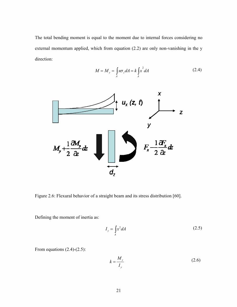
The total bending moment is equal to the moment due to internal forces considering no
external momentum applied, which from equation (2.2) are only non-vanishing in the y
direction:
(2.4) 2
y zA A
M M x dA k x dAσ= = =∫ ∫
Figure 2.6: Flexural behavior of a straight beam and its stress distribution [60].
Defining the moment of inertia as:
(2.5) 2y
A
I x dA= ∫
From equations (2.4)-(2.5):
(2.6) y
y
Mk
I=
21
and the cross sectional stress is given by:
(2.7)
yz
y
M xI
σ =
Using Hook’s law, the strain is given by:
(2.8)
yzz
y
M xE EI
σε = =
where E is Young’s modulus.
If is the displacement of the beam in x direction and the deflection is small, ( , )xu z t
, then the second derivative of the deflection which is approximately the
inverse of the radius of curvature r is given as:
( /xdu dx 1)
(2.9) 2
2
( , ) 1xu z tz r
∂≈
∂
The strain can be calculated as:
(2.10)
0
0
( )sin
dl dl r x d rd xdl r d r
θ θεθ
− − − −= = =
The Euler-Bernoulli law of elementary beam theory can be obtained by combining
equations (2.8) and (2.10),
(2.11) 2
2M E ( , )xy y
u z tIz
∂= −
∂
In the absence of external forces or bending moments, the equation of motion becomes:
(2.12)
and as the total moment has to be zero,
2
int2
( , )xu z tm Ft
∂=
∂ ∑
(2.13) int 0M =∑
22

The relationship between the bending moment and the force:
(2.14) M
The mass of the beam can be given as,
(2.15)
where ρ is the density of the beam, A is its cross sectional area and dz is its dimension
along the z- direction. Using equation (2.15), we can write the equation of motion (2.12)
as,
(2.16)
After substituting equation (2.11) we get the final equation of motion:
(2.17)
Using
(2.18)
and solving equation of motion (2.17) we get,
(2.19)
For a clamped-free cantilever, the boundary conditions at the clamped end are:
(2.20)
yxF
z∂
= −∂
zm Adρ=
22
2 2
( , ) yx Mu z tAt Z
ρ∂∂
= −∂ ∂
2 4
2 4
( , ) ( , ) 0x xy
u z t u z tA EIt z
ρ ∂ ∂+ =
∂ ∂
4
y
AEIρα =
1 2 3 4( , ) sin( ) cos( ) sinh( ) cosh( )xU z B z B z B z B zω α ω α ω α ω α ω= + + +
(0, ) 0 (0, ) 0 xx
dUUdz
ω ω= =
23

and at the free end (z = L) with no bending moments or shear forces acting on the beam
are:
(2.21) 2 3
2 3
( , ) ( , ) 0 0 x xd U L dU Ldz dz
ω ω= =
The first boundary conditions forces B2 = B4 and B1 = -B3, whereas applying the last
conditions the solution reduces to:
(2.22) 2 2cos( )cosh( ) 0sin( ) sinh( )
L LL L
α ω α ωα ω α ω
+=
−
There is no analytical solution but can be solved numerically using the substitution:
(2.23)
Lβ α ω=
The natural resonant angular frequencies can be calculated as,
(2.24)
2
2yiωi
EIL Aβ
ρ=
The moment of inertia of a beam with circular cross section is given by:
(2.25) 4
64yDI π
=
where D is the diameter of the beam and the inertia for rectangular cross section is:
(2.26)
3
12ywdI =
where w is the width and d is the thickness of the beam respectively. The final solution is
the same for the clamped - clamped and free- free beam with the only difference from the
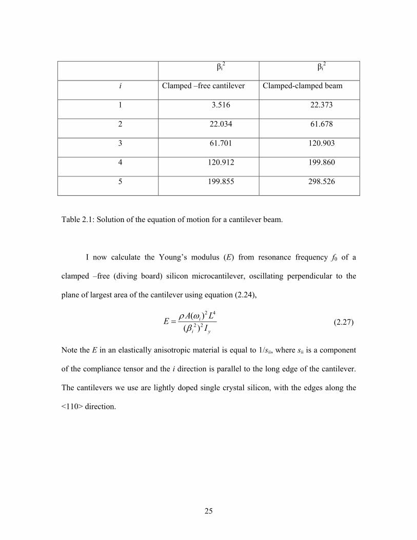
cantilever in the factor βi, given in the Table 2.1.
24
βi2 βi
2
i Clamped –free cantilever Clamped-clamped beam
1 3.516 22.373
2 22.034 61.678
3 61.701 120.903
4 120.912 199.860
5 199.855 298.526
Table 2.1: Solution of the equation of motion for a cantilever beam.
I now calculate the Young’s modulus (E) from resonance frequency f0 of a
clamped –free (diving board) silicon microcantilever, oscillating perpendicular to the
plane of largest area of the cantilever using equation (2.24),
2 4
2 2
( )( )
i
i y
A LEI
ρ ωβ
= (2.27)
Note the E in an elastically anisotropic material is equal to 1/sii, where sii is a component
of the compliance tensor and the i direction is parallel to the long edge of the cantilever.
The cantilevers we use are lightly doped single crystal silicon, with the edges along the
<110> direction.
25

Microcantilever Dimensions according to manufacturer (Mikromasch): Length: L = 350 [μm]
Width: w = 35 [μm]
Thickness: d = 2 [μm]
Area: A = wd
Material Properties of Cantilever:
Density: ρ = 2330 [kg/m3]
Resonant Frequency: f0 = 17.74 [kHz]
The resonant frequency (f0) of the Si microcantilever reported above is measured using
the Harmonic Detection of Resonance (HDR) technique (discussed in chapter 3). Hence,
using equations (2.26) and (2.27) with ω0 = 2πf0 we get,
2 40
2 2 2
12 (2 )( )Si
i
f LEd
ρ πβ
=
2 6 4
2 6 2 2
12(2330)(2 17,740) (350 10 ) 105.5(3.516) (2 10 )Si
kgE Gs m
π −
−
× × ×= =
×Pa
From Nye[61], for a cubic material,
( )2 2 2 2 2 211 11 12 1 2 1 3 2 3
44
1 12 2s s s l l l l l lsE⎛ ⎞= − − − + +⎜ ⎟⎝ ⎠
26
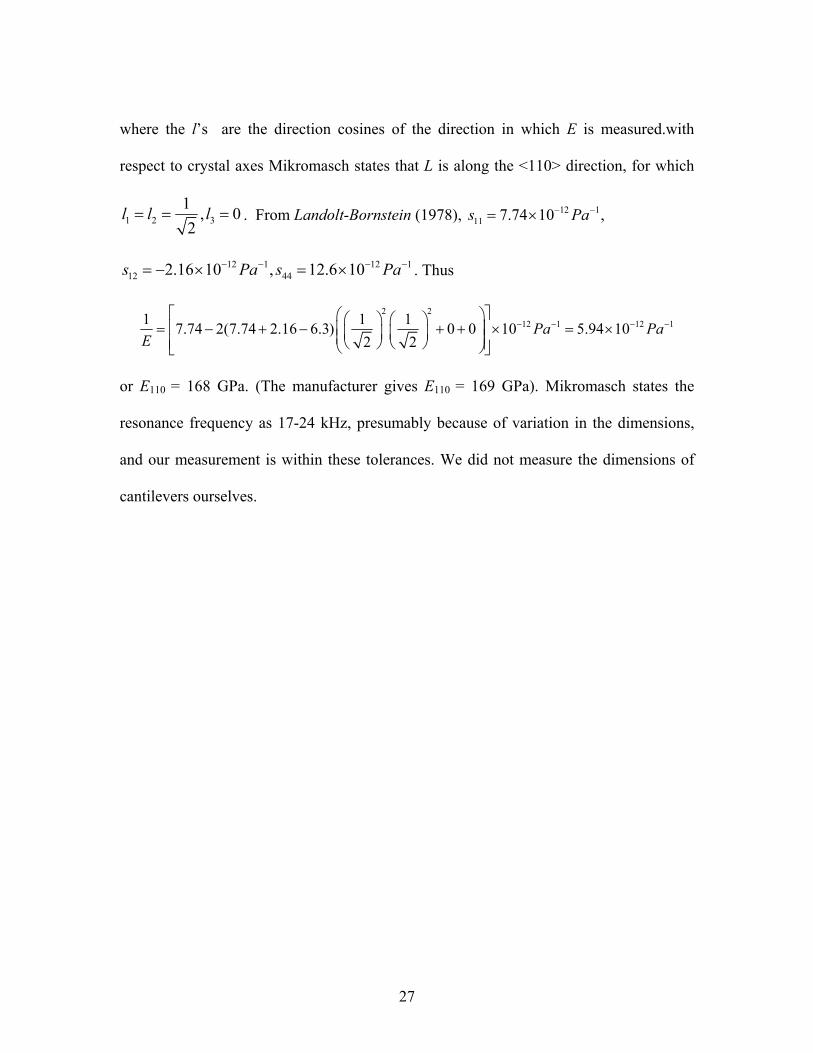
where the l’s are the direction cosines of the direction in which E is measured.with
respect to crystal axes Mikromasch states that L is along the <110> direction, for which
1 2 31 ,2
l l l= = = 0 a. From Landolt-Bornstein (1978), 12 111 7.74 10 ,s P− −= ×
12 1 12 112 442.16 10 , 12.6 10s Pa s− − −= − × = × Pa− . Thus
2 212 1 12 11 1 17.74 2(7.74 2.16 6.3) 0 0 10 5.94 10
2 2Pa P
Ea− − −
⎡ ⎤⎛ ⎞⎛ ⎞ ⎛ ⎞⎢ ⎥= − + − + + × = ×⎜ ⎟⎜ ⎟ ⎜ ⎟⎜ ⎟⎢ ⎥⎝ ⎠ ⎝ ⎠⎝ ⎠⎣ ⎦
−
or E110 = 168 GPa. (The manufacturer gives E110 = 169 GPa). Mikromasch states the
resonance frequency as 17-24 kHz, presumably because of variation in the dimensions,
and our measurement is within these tolerances. We did not measure the dimensions of
cantilevers ourselves.
27

CHAPTER THREE
USING ELECTRIC ACTUATION AND DETECTION OF OSCILLATIONS IN MICROCANTILEVERS FOR PRESSURE MEASUREMENTS
Introduction Cantilever structures are the simplest structures that can be easily micro-
machined, mass produced and integrated into (MEMS/NEMS) [60]. The
microcantilever’s response depends on any variable that changes the vibration of the
cantilever, and is measured as a change in the resonance frequency, amplitude, phase
and/or quality factor. These response characteristics of a microcantilever can serve as a
measure of a change in absolute pressure in the range of 10-4 to 103 torr. The major
difficulty in making these measurements is mostly the ancillary equipment such as lasers
or high magnetic fields that must be used. For these measurements it is advantageous if
the resonating system is portable and therefore a capacitive readout of the mechanical
vibration is ideal. In addition, the static capacitance between the microcantilever and a
counter electrode as well as the parasitic capacitance of the rest of the circuitry
overwhelm the signal making it difficult to detect the mechanical oscillations. The
various techniques currently available to overcome this difficulty mainly involve (i)
single electron transistors [62], which often operate at low temperatures, and (ii) sensing
elements such as comb drives along with on-chip circuitry [57, 63] which involve
intricate multi-element designs increasing the cost of production and probability to
breakdown. To this end, it would be very convenient to have the resonance of the
microcantilever actuated and detected electrostatically.
28

Harmonic Detection of Resonance
Recently, we have developed an electrical readout system using a technique called
the harmonic detection of resonance (HDR) [1, 2, 64]. In this technique, the
microcantilever is forced into resonance by electrostatic actuation applying an ac voltage
(Vac) with a dc offset (Vdc) to the counter electrode which is a tungsten (W) tip. The W
wire was etched in NaOH to form a sharp conical W tip [65]. The cantilever is aligned
near the counter electrode over the dark field microscope such that the long axis of the
cantilever intersects the axis of the conical tip, and the plane of the cantilever is parallel
to the nearby surface of the conical tip (see inset in Fig. 3.1). The electrical signal due to
the modulated charge created on the cantilever by the dynamic capacitance as well as the
electrostatic driving signal is measured by an A250 charge sensitive preamplifier. It is
also possible to measure the fA current going to and from the cantilever directly. The
charge induced on the cantilever is a function of the forcing voltages and the position of
the cantilever. This charge on a microcantilever has a rich harmonic structure and
measuring it at higher harmonics away from the driving frequency avoids the parasitic
capacitance problem. The lock-in amplifier detects the output of the A250 at the higher
harmonics of the frequency of the forcing ac voltage, which in turn is referenced to the
signal generator (Fig. 3.1). We have shown that this enables easy determination of the
resonance frequency of individual microcantilevers with a substantial signal to
background ratio. Using HDR, we have measured mechanical resonances (f0) in silicon
microcantilevers at 2nd, 3rd 4th , 5th and 6th harmonics [2]. This technique offers unique
29

benefits for devices, such as highly portable design, reduction in background signal, low
power consumption, and fast response.
In general, we are only concerned with the first mode of vibration. This is
because of the greatest tip deflection in the 1st mode facilitating measurement. Also, the
amplitudes of the higher modes are small at the driving frequencies used, in part because
the coupling to the electrostatic field is weaker for higher modes. Finally, the lock-in
amplifier used has a limited frequency range; making it difficult to measure the
harmonics of higher modes. Each mode of vibration has a particular natural frequency (f0)
and damping ratio. Note the distinction between modes and harmonics. The term
“harmonic”, which is defined as an integer multiple of some fundamental frequency is
very often confused with the modes of vibration. The confusion arises because for
doubly clamped structures, e.g. violin strings, the frequencies of higher modes of
vibration are all integer multiples of the first mode frequency, just as for harmonics. Thus
for doubly clamped systems, harmonic and modal frequencies are essentially
interchangeable. However, for cantilevers the frequencies of the higher modes are not
integer multiples of the first, and thus harmonic and modal frequencies are not
equivalent.
30

Figure 3.1: A schematic of the experimental set up using our harmonic detection of
resonance method for sensing pressure changes. The inset shows the geometry of the
cantilever with respect to that of the W tip.
Silicon microcantilevers have been extensively studied as sensors for pressure,
temperature, mass and viscosity measurements [14, 66-71]. The ongoing research in this
area mainly focuses on the resonance response as a function of pressure in different
regimes - the intrinsic regime, the molecular flow regime, the viscous regime, and
transition regimes in between. In the intrinsic regime (10-8 torr - 10-6 torr) due to the low
air pressure, air damping is insignificant compared to the intrinsic damping of the
vibrating cantilever itself. Hence the resonant frequency f0 and the quality factor Q are
31

nearly independent of air pressure p. The collisions of air molecules with the vibrating
cantilever cause the damping in case of the molecular region (10-6 torr – 10-1 torr). For
the viscous region (p > 10-1 torr), the velocity of the cantilever is always much smaller
than the speed of sound in the medium and hence we can consider air as a viscous fluid.
However, there can be turbulence, in which case the damping is roughly proportional to
the square of velocity [72]. In the molecular region, the dependence of Q on p can be
explained by the Christian model [73], which emphasizes that the Q is proportional to
1/p. Blom et al. mainly focuses on dividing the viscous regime into two zones, one with
Q independent of p and the other with Q proportional to 1/√p [71]. In this chapter, we
report the nonlinear dynamics of microcantilevers under different gases with varying
pressures at higher harmonics using HDR [2]. The use of different harmonics can enable
us to adjust the range of pressures over which the sensor has an efficacious response,
enhancing its sensitivity to a particular environment.
The main focus of this investigation is to conduct a characteristic study of a
resonating cantilever as a function of chamber pressure over six decades (10-3 torr – 760
torr) using the HDR technique described briefly in the previous paragraph [2]. The effects
of different gases: He, Ar, H2, and air are measured and are compared with theoretical
results. We performed a separate study to compare the 2nd and 3rd harmonic responses of
a silicon microcantilever as a function of p.
32

Quality factor (Q)
For a harmonic oscillator, the usual definition of the quality factor Q is
2 2 (stored vibration energy)energy dissipated per period
i
d
UQUπ π
= =
It is usually measured at the 1st harmonic of the power curve near resonance in a linear
system, that is, a simple harmonic oscillator (SHO). In case of our HDR technique, we do
not have a simple harmonic oscillator, nor is it easy to measure the first harmonic
response, as it is usually overwhelmed by parasitic capacitance signals. For an SHO, Q is
also equal to the resonant frequency (f0) divided by the full width at half maximum of the
resonance peak of a power vs. frequency plot. We will use the following definition of the
experimental quality factor QE for any harmonic and for cantilever motions that are
nearly that of a SHO as well as the motions in which the position of the cantilever affect
the spring constant and driving force.
0E
fQFWHM
= (3.1)
where FWHM is the full width at half maximum of the resonant peak of a squared
amplitude vs. frequency plot, for any harmonic. Although this is not the standard Q, it is
generally consistent with results predicted for a standard Q as discussed next.
Effect of damping on QE The equation of motion for a real system governed by the damping, a time
dependent force (F0) is given as,
33

2
02( ) ( ) ( ) cos( )x t x tm b kx t F
t ttω∂ ∂+ + =
∂ ∂
where m is effective mass of the 1st mode of vibration of the cantilever, b is damping
parameter, k is spring constant , x is the displacement of the cantilever. Further,
following Pippard [74] for a damped SHO, the quality factor is identical to QE defined
above and given as,
12EQ ω
ω′
=′′
,
where 2bm
ω′′ = and 2 2
20 2 2
2 2b k bm m m
ω ω ⎛ ⎞ ⎛ ⎞ ⎛ ⎞′ = − = −⎜ ⎟ ⎜ ⎟ ⎜ ⎟⎝ ⎠ ⎝ ⎠ ⎝ ⎠
,
Since we can determine ω0 and QE, we should be able to calculate the damping, b.
Note that we will have to plot the square of the amplitude vs. frequency to get QE. Thus
220 2
21 12 2
2
E
bmQ b
m
ωωω
⎛ ⎞− ⎜ ⎟′ ⎝ ⎠= =′′
220
22
2 22 2
0
2 20
2
22
42
4 22 2
2 4 2
E
E
E
bmQ
bm
b bQm m
bm Q
ω
ω
ω
⎛ ⎞− ⎜ ⎟⎝ ⎠=
⎛ ⎞⎜ ⎟⎝ ⎠
⎛ ⎞ ⎛ ⎞= −⎜ ⎟ ⎜ ⎟⎝ ⎠ ⎝ ⎠
⎛ ⎞ =⎜ ⎟ +⎝ ⎠
34
Since in our case QE >> 50, we can neglect the 2 in the denominator on the right side, and
get the damping b as,
0
E
b mQω
≈ (3.2)
Since we can directly determine angular resonant frequency (ω0) and QE, and estimate m
reasonably well, we can estimate the damping, b, with the caveat that our systems are not
linear and we use harmonics other than the first.
Pressure dependence of the quality factor The viscous region: For the viscous region, Hosaka et al. gave a direct evaluation
of the quality factor [75]
( ) ( )
20
20
26 3 2 2
bp
dwQw w M RT
ρ ωpπμ π μ
=+ ω
(3.3)
where d is the thickness, w the width of the cantilever, μ the dynamic viscosity, M the
molecular mass of the gas molecules and ρb the density of the cantilever beam R, T and p
are the gas constant, the absolute temperature and pressure respectively.
As emphasized by Blom et al. we can see from equation (3.3) the first (low
pressure) part of the viscous region is almost independent of pressure however when the
pressure increases, the quality factor prominently shows 1/√p dependence.
35

The molecular region: In the molecular regime the quality factor can be written as
[66],
0 14 2
bp
d RTQM p
ρ ω π= (3.4)
which clearly indicates its 1/p dependence taking into account the collisions between the
gas molecules and the vibrating cantilever. The total quality factor (QE) of the system can
be given as
1 1 1
E pQ Q Q= +
Si
(3.5)
where Qp is the pressure dependent quality factor and QSi is the pressure independent
intrinsic quality factor. Simplifying equation (3.5) the experimental quality factor in the
molecular regime can be written as,
11
E
C p CQ
= + 2 (3.6)
where C1 is the slope of a plot of 1/QE vs. p and C2 is one over the intrinsic quality factor
of the cantilever (QSi). The parameter (C2) can be used as a measure of the thermal and
defect properties of materials.
Resonant frequency and spring softening Taking into account the softening of the effective spring constant of the system
from k to k´ [60], the resonant angular frequency of the cantilever driven into resonance
using HDR is given by [76],
36

0km
ω′′ = (3.7)
with
(3.8)
where
(3.9)
where the force (Fc) is proportional to the derivative of the capacitance (C) as a function
of the position x of the cantilever.
Experimental Setup
The microcantilevers used in this pressure study are gold-coated silicon tipless
microcantilevers from Micromasch, typically 35 µm wide, 2 µm thick and 350 µm long.
The microcantilever and a sharpened tungsten tip (acting as a counter electrode) are glued
down on the chip carrier in a parallel geometry with ~10 μm gap distance. We used HDR
to measure the response of a silicon micro-cantilever (f0 = ~17 - 21 kHz) mounted on a
chip carrier [1, 2, 64]. The experimental setup consists of an A250 charge amplifier, a
signal generator, a dc power supply, and a lock-in amplifier as explained before in Fig.
3.1. This chip carrier was then plugged into a board mounted inside a glass chamber
which was subjected to changes in pressure and environments. The various experiments
carried out on these microcantilevers can be divided into three groups:
22 2
20
1½ 2 cos( ) [1 cos(2 )2
Cdc dc ac ac
x
dF d C V V V t V tdx dx
ω ω=
⎡ ⎤= − + + +⎢ ⎥
⎣ ⎦]
ck k dFdx′ = −
37

(i) Study the effect of pressure on the response of a vibrating cantilever as a
function of environment. Using a pump station, the chamber pressure was varied from
10-3 torr to ambient pressure (760 torr) under different environments such as air and He.
The low pressures (< 10-3 torr) are measured using a hot cathode gauge, and (KJLC BDG
Series) Bourdon dial gauges are used around ambient pressure. The thermocouple
pressure gauge is used for in-between pressures.
(ii) Study the impact of molecular mass on a different cantilever’s vibration by
back filling the glass chamber (cf. Fig. 3.1) at 760 torr with H2, He, air and Ar.
(iii) A separate cantilever of the same size was used to study the cantilever’s
vibration at the 2nd and 3rd harmonics under different chamber pressures in He. We are
working with the gases for which we expect negligible physical or chemical absorption or
effects due to their dielectric constant. Further, all the measurements are carried out at
room temperature and the damping of the vibrating cantilever can be attributed to the
internal friction in the cantilever (intrinsic damping), the friction at the support and the
surrounding gas.
Results and Discussion
(I) Response to pressure
We started with a new and clean microcantilever having a QE ~ 60 in ambient air
at atmospheric pressure with a gap distance of 8 μm. The water vapor present in the
ambient air has been shown to have an insignificant effect on our results. The
38

microcantilever demonstrated very high QE ~ 10,000 at 10-3 torr, as shown in Fig. 3.2
which saturated at pressures below 10-3 torr (not shown). While studying a different
cantilever at lower pressures, the effective spring constant decreased causing the resonant
frequency to decrease as shown in Fig. 3.3(a) (equation (3.7)). This could be attributed to
the greater amplitudes (and thus higher QE) at these pressures that lead to the cantilever
spending more time close to the counter electrode thereby resulting in the spring
softening (equation (3.8)). There may also be a shift in resonant frequency due to the
change in damping. A similar trend was observed in the case of a He environment (Fig.
3.3(b)). The smaller atomic mass of He caused relatively lower damping, contributing to
the larger amplitudes and the higher QE along with the decrease in the resonant frequency
compared to air (Figs. 3.3(a) and 3.3(b)). At ambient pressure the damping parameter is
3.21×10⁻⁸ Nsm-1 under a He environment (calculated using equation (3.2)). 1/QE showed
an approximately linear response (shown by the dotted line) to pressure in the molecular
region as predicted by equation (3.6) in both air and He environments. The calculated
value of constant C2, corresponding to 1/QSi, is 1.35×10⁻⁴ in both air and He and thus is in
good agreement with the values reported in the literature (Q-1 = 3×10⁻⁴ to 1.24×10⁻⁴) (see
Fig. 3.4) [60]. Similarly the slope of the 1/ QE vs. pressure plot (C1) in the molecular
region is 7×10⁻⁴ torr -1 in He and the slope calculated using equation (3.4) is 1.43×10⁻⁴
torr-1. Hence the experimental results are consistent with the theoretical model
calculations, giving some justification for using our QE for the usual Q. We also
compared QE and the normalized variation of resonant frequency (f0) as a function of
pressure with the results presented by Bianco et al. [66] (Figs. 3.5(a), 3.5(b)). Similar
39

trends are observed in both cases. It is the fractional change in resonant frequency or
quality factor which determines the utility of the cantilever as a pressure gauge. In Fig.
3.5 (a) the log scales indicate the fractional changes in quality factor equally well for the
two results. Our data followed their experimental values very well (although with some
loss in sensitivity) in spite of the difference in the excitation and detection schemes of the
microcantilever in the two studies (Fig. 3.5(a)). For Fig. 3.5(b) little change in f0 is
observed with pressure changes. Bianco et al. [66] have a larger fractional change in f0
near atmospheric pressure. But in neither their work nor ours is there a sufficient change
in f0 to be useful as a gauge. In both techniques, the variation is small, but particularly so
in the nonlinear HDR system. We get comparatively higher amplitudes at low pressures,
as well as a decrease in f0 [2]. A possible reason for this is that the nonlinearities in our
system make higher amplitudes shift the apparent f0 to lower frequencies, thus canceling
the increase seen by Bianco et al. [2].
40

Figure 3.2: Amplitude (bullets) and phase (crosses) of the cantilever near the resonance
frequency for 760 (blue) and 3E-3 torr (red) when measured at the 2nd harmonic (Vdc = 9
V, Vac = 5 V) with 8 μm gap distance. The large change in the 2nd harmonic signal shows
that the HDR technique is a viable method for pressure sensing.
41
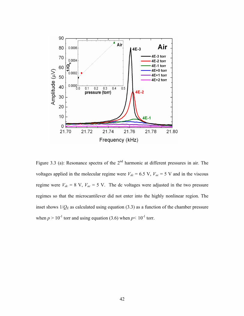
Figure 3.3 (a): Resonance spectra of the 2nd harmonic at different pressures in air. The
voltages applied in the molecular regime were Vdc = 6.5 V, Vac = 5 V and in the viscous
regime were Vdc = 8 V, Vac = 5 V. The dc voltages were adjusted in the two pressure
regimes so that the microcantilever did not enter into the highly nonlinear region. The
inset shows 1/QE as calculated using equation (3.3) as a function of the chamber pressure
when p > 10-1 torr and using equation (3.6) when p< 10-1 torr.
42

Figure 3.3 (b): Resonance spectra at the 2nd harmonic at different pressures in a helium
environment. In the molecular region voltages applied were Vdc = 6.5 V, Vac = 5 V and in
viscous region were Vdc = 8 V, Vac = 5 V. Note the higher sensitivity of the response in a
lighter gas. The inset shows 1/QE as a function of the pressure in a He environment.
43
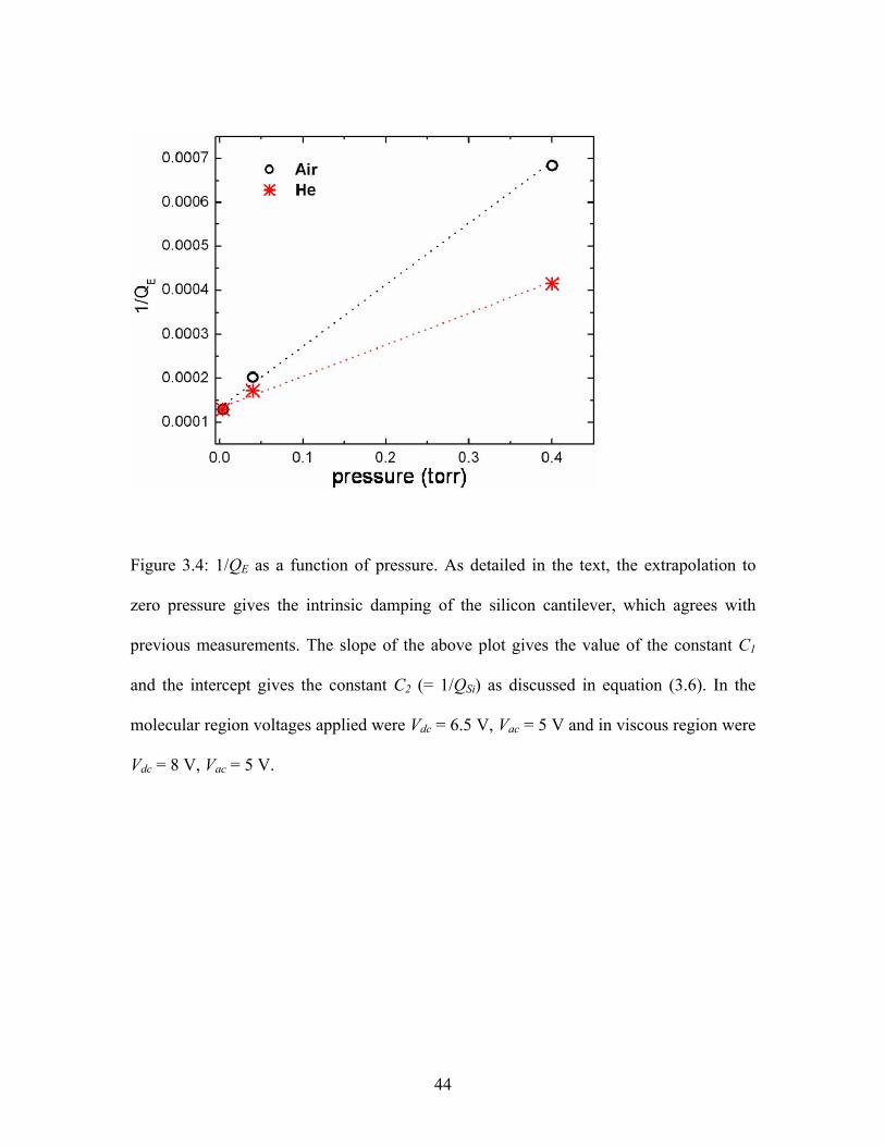
Figure 3.4: 1/QE as a function of pressure. As detailed in the text, the extrapolation to
zero pressure gives the intrinsic damping of the silicon cantilever, which agrees with
previous measurements. The slope of the above plot gives the value of the constant C1
and the intercept gives the constant C2 (= 1/QSi) as discussed in equation (3.6). In the
molecular region voltages applied were Vdc = 6.5 V, Vac = 5 V and in viscous region were
Vdc = 8 V, Vac = 5 V.
44
Figure 3.5 (a): Comparison of the experimental results (shown by red squares, left hand
axis) for QE as a function of pressure using HDR (red squares) and Q as measured by
Bianco et al. [66] (shown by blue circles, right hand axis) using piezoelectric excitation
and optical detection. In the molecular region voltages applied were Vdc = 6.5 V, Vac = 5
V and in viscous region were Vdc = 8 V, Vac = 5 V.
45

Figure 3.5 (b): Our experimental results (shown by red squares, left hand axis) for the
normalized variation of resonant frequency as a function of pressure using HDR and the
experimental data presented by Bianco et al. [66] (shown by blue circles, right hand axis)
in the viscous region. In the molecular region voltages applied were Vdc = 6.5 V, Vac = 5
V and in viscous region were Vdc = 8 V, Vac = 5 V.
(II) Impact of the gas environment
Equations ((3.3) and (3.4)) show that Q is inversely proportional to the square
root of the mass of the gas inside the chamber. It can be seen in Figs. 3.6(a) and 3.6(b)
that the resonant frequency, amplitude, and thus the quality factor changed with the
change in environment at ambient pressure (760 torr). A different silicon microcantilever
46
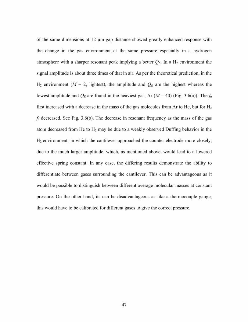
of the same dimensions at 12 μm gap distance showed greatly enhanced response with
the change in the gas environment at the same pressure especially in a hydrogen
atmosphere with a sharper resonant peak implying a better QE. In a H2 environment the
signal amplitude is about three times of that in air. As per the theoretical prediction, in the
H2 environment (M = 2, lightest), the amplitude and QE are the highest whereas the
lowest amplitude and QE are found in the heaviest gas, Ar (M = 40) (Fig. 3.6(a)). The f0
first increased with a decrease in the mass of the gas molecules from Ar to He, but for H2
f0 decreased. See Fig. 3.6(b). The decrease in resonant frequency as the mass of the gas
atom decreased from He to H2 may be due to a weakly observed Duffing behavior in the
H2 environment, in which the cantilever approached the counter-electrode more closely,
due to the much larger amplitude, which, as mentioned above, would lead to a lowered
effective spring constant. In any case, the differing results demonstrate the ability to
differentiate between gases surrounding the cantilever. This can be advantageous as it
would be possible to distinguish between different average molecular masses at constant
pressure. On the other hand, its can be disadvantageous as like a thermocouple gauge,
this would have to be calibrated for different gases to give the correct pressure.
47

Figure 3.6 (a): Dependence of QE on the molecular mass of the surrounding gas measured
at the 2nd harmonic at ambient pressure with Vdc = 9 V, Vac = 10 V at 12 μm gap distance.
48

Figure 3.6 (b): Resonance frequency spectra under different gas environments at the 2nd
harmonic at ambient pressure with Vdc = 9 V, Vac = 10 V.
(III) Response at higher harmonics of the modulated charge
The systematic study of the responses of a different cantilever at higher harmonics
in a He environment is conducted. It is observed that the signal amplitude was higher at
the 2nd harmonic compared to the 3rd harmonic at the same pressure [2] (Figs. 3.7(a) and
3.7(b)). At the 3rd harmonic, a signal is measured at three times the driving frequency,
leading to lower parasitic pickup due to the measurement further away from the driving
frequency. Thus due to lower background signal, QE is higher at the 3rd harmonic than at
49
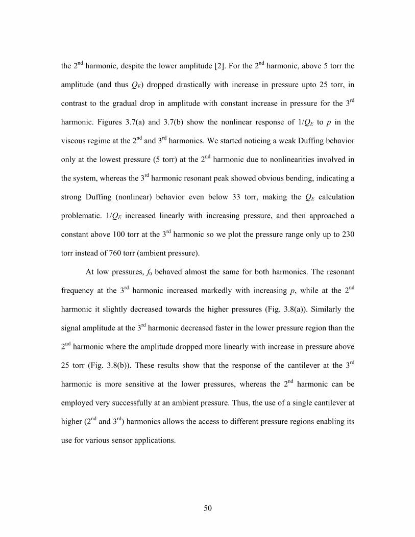
the 2nd harmonic, despite the lower amplitude [2]. For the 2nd harmonic, above 5 torr the
amplitude (and thus QE) dropped drastically with increase in pressure upto 25 torr, in
contrast to the gradual drop in amplitude with constant increase in pressure for the 3rd
harmonic. Figures 3.7(a) and 3.7(b) show the nonlinear response of 1/QE to p in the
viscous regime at the 2nd and 3rd harmonics. We started noticing a weak Duffing behavior
only at the lowest pressure (5 torr) at the 2nd harmonic due to nonlinearities involved in
the system, whereas the 3rd harmonic resonant peak showed obvious bending, indicating a
strong Duffing (nonlinear) behavior even below 33 torr, making the QE calculation
problematic. 1/QE increased linearly with increasing pressure, and then approached a
constant above 100 torr at the 3rd harmonic so we plot the pressure range only up to 230
torr instead of 760 torr (ambient pressure).
At low pressures, f0 behaved almost the same for both harmonics. The resonant
frequency at the 3rd harmonic increased markedly with increasing p, while at the 2nd
harmonic it slightly decreased towards the higher pressures (Fig. 3.8(a)). Similarly the
signal amplitude at the 3rd harmonic decreased faster in the lower pressure region than the
2nd harmonic where the amplitude dropped more linearly with increase in pressure above
25 torr (Fig. 3.8(b)). These results show that the response of the cantilever at the 3rd
harmonic is more sensitive at the lower pressures, whereas the 2nd harmonic can be
employed very successfully at an ambient pressure. Thus, the use of a single cantilever at
higher (2nd and 3rd) harmonics allows the access to different pressure regions enabling its
use for various sensor applications.
50
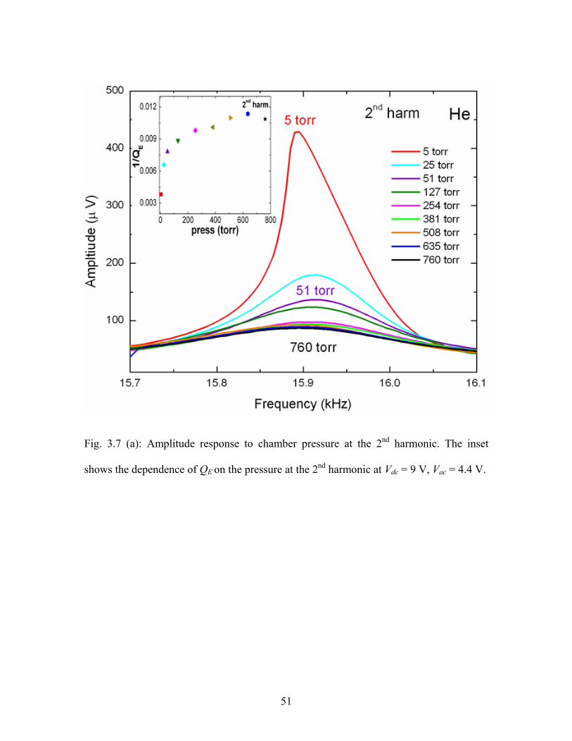
Fig. 3.7 (a): Amplitude response to chamber pressure at the 2nd harmonic. The inset
shows the dependence of QE on the pressure at the 2nd harmonic at Vdc = 9 V, Vac = 4.4 V.
51

Figure 3.7(b): Amplitude response to chamber pressure at the 3rd harmonic. The inset
shows the dependence of QE on the pressure at the 3rd harmonic at (Vdc = 9 V, Vac = 6.2
V).
52

Figure 3.8 (a): Comparison of the resonant frequency of the cantilever as a function of
pressure at the 2nd (Vdc = 9 V, Vac = 4.4 V) and 3rd (Vdc = 9 V, Vac = 6.2 V) harmonics in a
He environment. The different harmonics may allow the measurement of the pressure
over a larger region than a single harmonic.
53

Figure 3.8 (b): Comparison of amplitudes at f0 of the cantilever as a function of pressure
at the 2nd (Vdc = 9 V, Vac = 4.4 V) and 3rd (Vdc = 9 V, Vac = 6.2 V) harmonics in a He
environment. The red line is used as guide to the eye for low pressures at 2nd harmonic
and blue line is used for 3rd harmonic.
Conclusions HDR offers unique features, particularly electrostatic excitation and detection.
The microcantilever demonstrates a quality factor of ~10000 at 10-3 torr, and a usable
response in the range from 10-3 to 103 torr. Here we have shown that currently our sensor
is fairly sensitive compared to the one presented by Bianco et al [66]. The nonlinearities
54

55
present in HDR make it special and more useful than the rest of the other resonance
detection methods. While the HDR method may not be as sensitive as other techniques,
the other techniques are often more bulky, expensive, and prone to errors. Furthermore,
it may also be easier to fabricate a device that is all silicon than one which contains
piezoelectric and laser components. The responses of QE to pressure in the viscous and
molecular regions are similar to those measured with a more linear system that used
piezoelectric excitation and optical detection [66]. The experimental results are in
reasonable agreement with theoretical calculations, despite the nonlinearities involved: Q
is inversely proportional to (i) pressure in the molecular region and (ii) the square root of
the mass of the gaseous medium. At the 3rd harmonic, the cantilever showed a stronger
dependence on p in the low pressure regime, whereas an almost uniform and linear
response was observed at the 2nd harmonic over the entire pressure range. The benefit of
switching between different harmonics depending upon the pressure regime can provide
us with a higher flexibility as a pressure sensor. We are exploring the possibility of using
carbon nanotubes/nanostructures which we expect will have lower intrinsic damping for
sensing even lower pressures.
.

CHAPTER FOUR
ULTRA-SENSITIVE DUFFING BEHAVIOR OF A MICROCANTILEVER
Introduction
Micro electro-mechanical systems (MEMS) enable the fabrication of fully
integrated sensors and actuators for continuously growing range of applications. A
characteristic feature of many MEMS devices that has recently received much attention is
the nonlinear response to ac driving signals [77]. It has been postulated that nonlinear
spectral features may allow a greater dynamic range and enhance the sensitivity [78]. We
have been studying the behavior of electrostatically driven and measured cantilevers and
noticed that it is possible to drive them hard enough to observe Duffing-like jumps in
their amplitude- frequency behavior [74]. Typically in a Duffing resonator, above some
critical driving amplitude, the response becomes a double-valued function of frequency in
some finite frequency range. The presence of the bistable region results in a dramatic
jump transition from a near-zero solution to one of the high amplitudes. Using the
Duffing-like behavior of microcantilever provides us with the ability to engineer the
ultra-high-sensitivity of this bistability [79, 80]. This Duffing-like behavior could be
useful in sensing technologies [81].
Nonlinearity effects on resonance are often described using the classical Duffing
equation [82],
56

2 32 (o )x x x x Eω εγ εα+ = − − + t (4.1)
where ε is a small parameter, E is an externally applied force, γ is positive viscous
damping, ω0 is the angular resonant frequency and α can be either positive (hard spring)
or a negative (soft spring) constant. Here
( ) cosE t Z= tΩ (4.2)
where Ω is the angular driving frequency and Z is a constant. Equation 4.1 can be solved
by either the method of multiple scales [83] or the method of harmonic balance [82].
However, we do not see the typical Duffing behavior, but rather the behavior which
mimics it which could be because of more complex nonlinearities than the classical case.
Henceforward we will call these Duffing like effects simply the Duffing behavior.
Currently very little is known about the physical mechanisms underlying the Duffing
behavior of harmonics other than the first. The published literature mainly focuses on the
theoretical understanding of the mechanisms involved in Duffing behavior and proposes
its application as a sensor. But we did not find a report that experimentally demonstrates
a sensing based on the Duffing behavior.
In this chapter we investigate the properties of an electrostatically driven
microcantilever exhibiting Duffing-like behavior using HDR technique. Its potential use
as a highly sensitive sensing platform is discussed. We study the effect of damping on the
Duffing behavior of a microcantilever in hydrogen, air and vacuum. We also demonstrate
the tuning of the transition frequency of a Duffing resonator in both the forward and
backward directions by voltage changes and evaluate some potential applications
associated with different regimes of frequency tuning. The response of the higher
57

harmonics of the measured charge on the cantilever induced by an ac voltage that drives
the counter electrode is investigated. In particular, we trace the Duffing behavior at the
higher harmonics (up to the 6th harmonic) as a function of gap distance between the
cantilever and counter electrode.
Mathematical Model
A literature survey shows that the theoretical interpretations of basic Duffing
behavior and the related nonlinearities have been extensively used in MEMS devices [78,
84-86]. We will present in this chapter a simple mathematical model of the nonlinearities
present in our system leading to Duffing behavior. First the experimental set up for
Duffing study using HDR method is discussed [2]. A silicon microcantilever and a
tungsten tip (acting as a counter electrode) were brought into a parallel configuration with
a gap distance (s) of 8-10 μm inside an evacuable glass chamber (as discussed in previous
chapter in Fig. 3.1). We studied its Duffing behavior by driving the microcantilever into
the nonlinear regime with appropriate ac and dc voltages applied to the counter electrode
using our HDR setup.
58

Equation of motion
For simplicity, here we assume that the amplitude of the 1st mode is given by the
single coordinate x [83], and the force can be given as,
2
2
22
2
12
F mad xF mdtd dF CV mdx dt
x
=
=
⎛ ⎞= − =⎜ ⎟⎝ ⎠
where the capacitance and the voltage 2
0 1 1 ....C C C x C x′ ′′= + + + cos( )dc acV V V t= + Ω
Hence, the Coulomb force FC on our cantilever can be written as the spatial derivative of
the Coulomb energy [2]:
2
2 2
[½ ( cos( )) ] /1 1 2 cos( ) [1 cos(2 )]2 2
C dc ac
dc dc ac ac
F d C V V t dxdCV V V t V tdx
= + Ω
= + Ω + + Ω (4.3)
where C is the capacitance of the cantilever-counter electrode system, and Ω is the
angular driving frequency.
When driven by these oscillatory and static voltages, the cantilever is forced
according to equation (4.3). This not only creates a force with two harmonically related
frequencies, f and 2 f, but also adds the nonlinearities due to the roughly 1/x2 dependence
of the capacitance. This leads to a significant change in the spring constant with applied
voltages and the presence of many harmonics in the deflection, as well as subharmonic
resonances.
59

For an electrostatically driven cantilever, we can write
2
2 Cd x dxm k
dtdtγ+ + =x F (4.4)
where m is the effective mass of the cantilever, k the effective spring constant and γ the
damping constant when the cantilever is vibrating in its first mode. The capacitance in
(4.3) can be expanded in a Taylor series in terms of the deflection.
20 1 2
1( , ) ( ) ( ) ...2!
C x t C C x t C x t≈ + + + (4.5)
where 0
n
n nx
CCX =
∂=
∂. Then equation (4.4) becomes
2
02
2 2 21 2 3
...
1 1 1( ...) 2 cos( ) [1 cos(2 )]2 2 2dc dc ac ac
d x dx Fm kx F xdt xdt
C C x C x V V V t V t
γ ∂+ + = + +
∂
= + + + Ω + + Ω (4.6)
The time independent term on the right involving C1 amounts to a zero shift and can be
eliminated with the substitution
2 21
1 / 22dc acx V V Cζ ⎛ ⎞= − +⎜ ⎟
⎝ ⎠k (4.7)
The term involving C2 is equivalent to a softening of the spring constant as the cantilever
approaches the counter-electrode. If we set
2
2 2
2 0 ...1 12 2dc ac
Ck V V ζκ
ζ =∂
= − + +∂
⎛ ⎞⎛ ⎞⎜ ⎟⎜ ⎟
⎝ ⎠⎝ ⎠ (4.8)
we can write the equation of motion as
( ) ( )2
2 3 22 3 42
1 1 1( ...) cos c2 6 2dc ac acm C C C V V t V
ttζ ζγ κζ ζ ζ ζ∂ ∂ os 2 t⎡ ⎤+ + = + + Ω + Ω⎢ ⎥∂∂ ⎣ ⎦
(4.9)
60

From equation (4.9) we can see that (i) the effective spring constant is affected by the
applied ac and dc potentials; and (ii) a quadratic term 23
12
C ζ and a cubic “Duffing” term
34
16
C ζ are present in the equation of motion. Note that there are also terms involving ζn
in κ. Since the cantilever resonates nonlinearly due to the geometry of the electrodes,
when the deflection ( )x t is expanded as a Fourier series given by,
1( ) cos( )
N
n nn
x t A n t δ=
= Ω +∑ (4.10)
many of the An’s will be finite. There may also be an additional cubic nonlinearity due to
the elastic properties of the beam and nonlinear damping [80].
The response curves for our cantilevers have two stable states due to these
nonlinearities (Fig. 4.1), which lead to the so-called “jump” phenomena [83]. When the
driving voltage frequency is slowly increased at constant amplitude, the response
amplitude will jump up at a frequency less than the resonance frequency (f0) that is
measured at low amplitude. The response amplitude will also jump down at a frequency
less than (f0) when the frequency is decreased from well above f0. One speaks of “hard”
and “soft” springs, in which the dynamic spring constant kd = dF/dx increases or
decreases as x increases. For hard springs, the resonance curve bends toward higher
frequency. For soft springs, such as those of our experiments, the resonance peak bends
toward lower frequencies. In the frequency domain in which two stable steady-state
solutions exist, the initial conditions determine which of these represents the actual
61

response of the system. Thus, in contrast with linear systems, the steady-state solution of
a nonlinear system can depend on the initial conditions [83].
Duffing Mechanism
Figure 4.1 represents the stable steady state solutions under different excitation
amplitudes. Referring to Fig. 4.1 we define some terminologies in the A vs. f curves
which we use in the experimental data analysis. In the first case where the excitation
amplitude is less than the critical amplitude, only one solution exists, and no bistability is
possible (Fig. 4.1(a)). For the case when the excitation amplitude equals the critical
amplitude, the system is on the edge of the bistability, and there exists one point where A
vs. f has an infinite slope showing incipient Duffing (Fig. 4.1(b)). In the case when the
excitation amplitude is greater than the critical amplitude the system is in the bistable
regime having three possible solutions over some range of frequencies. Two of these
solutions are stable. With increasing frequency the solution jumps from the low
amplitude stable solution (region I) to another high amplitude stable solution (as shown
by solid arrows) bypassing the unstable (experimentally unobservable) solution (shown in
red in region II). The large amplitude solution is stable and decreases with increasing
driving frequency f and finally enters into region III. In region (III) the system has only
one stable solution which with decreasing frequency bifurcates into a stable solution and
an unstable (red curve) solution. This stable solution grows in amplitude higher than the
stable solution accessible with increasing frequency as f continues to decrease (region II).
When the slope becomes infinite, this stable solution drastically collapses to the low
62

amplitude solution which is stable again (shown by dashed arrows in region I). Figure
4.1(c) shows the expected behavior in the 1st harmonic for a large third order non-
linearity [85].
Figure 4.1: Cartoon of steady state solutions under different excitation amplitudes
showing three stages of Duffing behavior [78]. The natural resonance frequency (f0) as a
function of A is shown by the blue line which differs from the f.
63
Experimental Setup
For this study we have used commercially available, one side gold-coated, tipless
microcantilevers from Micromasch, typically 35 µm wide, 2 µm thick and 350 µm long.
All experiments described in this manuscript are performed at room temperature and on
the same cantilever. The response of the resonating microcantilever is compared in air,
hydrogen and low vacuum (5 torr) to understand the effect of damping on Duffing
behavior. Furthermore, we record the Duffing behavior at higher harmonics (from 3rd to
6th) of the induced charge on the cantilever at two different gap distances between the
cantilever and counter electrode (4 μm and 8 μm). Since the non-linearities are sensitive
to small changes in geometry, the reproducibility of the results is checked. The sensitivity
of our Duffing resonator is measured by (i) pumping down the chamber to 5×10⁻⁵ torr (ii)
changing the pressure to 7×10⁻⁵ torr, the least change that we could make with our
experimental set up, triggering the Duffing behavior by this change in pressure.
Results and discussion
(I) Effect of ac - dc voltages on Duffing behavior
At the 1st harmonic, the detected resonance signal is overwhelmed by the
background signal due to the parasitic capacitance and manifests itself as a small peak at
the resonance frequency of the cantilever [2]. At the second and higher harmonics of the
driving frequency (f), the signal stemming from the parasitic capacitance is avoided,
64

permitting the detection of resonance with good signal to background ratios [2].
Interestingly, the Duffing behavior is more visible and prominent at the 3rd harmonic than
at the 2nd harmonic in air [3]. Hence all the experimental results were recorded at the 3rd
and higher harmonics of the ac voltage applied to the counter electrode. The ac voltage
applied to the counter electrode is swept with both increasing and decreasing f. Using a
dark field microscope, we estimate that the cantilever deflection amplitude is roughly one
quarter of the gap distance with an 8 μm gap distance between cantilever and the counter
electrode at 8 Vdc and 5 Vac. As seen in Fig. 4.2(a) at Vac = 2 V and Vdc = 8.5 V under
vacuum (5 torr), Duffing behavior is not observed. A polar plot with the amplitude as the
radius and the phase of the lock–in amplifier as the angle for the first harmonic of a
damped SHO is nearly a circle starting and ending on the origin. It is traversed counter
clockwise with increasing f and starts along the 180˚ axis. We find that the signals at
higher harmonics also give a similar circle under the experimental conditions described in
Fig. 4.2(a). Fig. 4.2(b) is a polar plot of the 2 Vac data of Fig 4.2(a), mapped through the
transition with both increasing and decreasing f. Note that the circle starts and finishes
off the origin. This offset is due to the presence of a coherent background signal present
in our experimental setup. The circle seen is the vector sum of the background signal and
the signal from the cantilever. The initial dip in the amplitude vs. frequency plot (Fig.
4.2(a)) is then seen to be due to the vector sum of the signal and the background and the
dip is shown by the black arrow in the polar plot (Fig. 4.2(b)). Such a dip was not seen in
case of hydrogen or air. The inset in each of the following figures is a polar plot of the
data in the main panel. As the ac voltage was increased to 3 V, Duffing behavior is
65

observed for both increasing and decreasing f. Thus, consistent with the discussions on
Equation of Motion, Vac is one of the key parameters for inducing Duffing behavior. The
polar plots consist of circular arcs at high and low f when the nonlinearities are large
enough to give rise to a Duffing behavior. These arcs are connected by the straight lines
at the Duffing jumps (Fig. 4.2(c)). As the nonlinearities grow the decreasing frequency
arc changes its curvature as shown in Fig. 4.2(c). Similar Duffing behaviors are seen
under various experimental conditions, and are summarized in table 4.1. The
experimental results are detailed in subsequent figures.
(a)
66

(b)
(c)
67

Figure 4.2: (a) Frequency spectra under vacuum. Dark circles are used for increasing and
light circles for decreasing f. At Vac = 2 V, there are no Duffing jumps. Increasing Vac to
3 V gives a spectrum showing Duffing jumps. The circled points are for comparison with
Figs. 4.2(b) and 4.2(c). The points S and M are the start and maxima of the amplitude
jumps in both amplitude (Fig. 5.2(a)) and polar (Fig. 5.2(c)) plots with increasing f.
(b) Data at 2 Vac from Fig. 4.2(a) in a polar plot in which the angle is the phase and the
radius is the amplitude of the response with increasing (dark circles) and decreasing (light
circles), f as a parameter. Tracing the vector amplitude shows why there is a dip in the
amplitude near resonance in the amplitude vs. Ω spectrum shown by the black arrow.
(c) Data at 3 Vac from Fig. 4.2(a) in a similar polar plot.
Figure Gas # of Harm
Gap size (μm)
Vac (V)
Vdc (V)
Fup(kHz)[∆A (μV)] Fdown (kHz) [∆A (μV)] Step size (kHz)
Fig. 3 (2Vac) vacuum 3 10 2 2 none none 0.01 Fig. 3 (3Vac) vacuum 3 10 3 3 15.97 [160] 15.79 [500] 15.89 [60] 0.01 Fig. 4 vacuum 3 10 2.6 8.5 15.98 [100] 15.86 [340] 15.8 [465] 0.01 Fig. 5 H2 3 10 7 8.5 15.86 [235] 15.79[450] 15. 7 [535] 0.001 Fig. 6 air 3 8 9.75 9.6 15.45 [410] 15.42 [410] 0.01 Fig. 7 air 4 8 9.75 9.6 15.44 [170] 15.42 [160] 0.01 Fig. 8 air 5 8 9.75 9.6 15.43 [55] 15.44 [43] 0.01 Fig. 9 air 6 8 9.75 9.6 15.46 [27] 15.44 [23] 0.01 Fig. 10 air 3 4 3 8.5 14.3 [160] 13.7 [140] 12.5 [220] 0.1 Fig. 11 air 4 4 3 8.5 13.9 [58] 14.1 [17] 13.7 [155] 12.5 [120] 0.1 Fig 12 air 5 4 3 8.5 13.8 [95] 14.3 [95] 13.4 [97] 12.3 [93] 0.1 Fig. 13 air 6 4 3 8.5 13.8 [8] 14.2 [8] 13 .5 [7.5] 12.2 [9] 0.1
Table 4.1: Summarizing Duffing behavior under various experimental conditions.
The polar plots corresponding to amplitude data shown in Fig. 3.7(b) at 3rd
harmonic is shown in Fig. 4.2 (d) at various pressures. It started with a perfect circle (as
expected) at 230 torr slowly growing in amplitude at lower pressures and then leading to
68

ellipsoidal at 33 torr showing incipient Duffing behavior. Finally we observed circular
arcs connected by straight lines exhibiting strong Duffing behavior at 5 torr.
Figure 4.2 (d): Data corresponding to Fig. 3.7 (b) in polar plot under vacuum at 3rd
harmonic (Vdc = 9 V, Vac = 6.2 V).
(II) Effect of damping on Duffing behavior
The response of the microcantilever at the 3rd harmonic under vacuum (5 torr) and
hydrogen (760 torr) with a 10 μm gap distance is shown in figs. 4.3 and 4.4. The
microcantilever showed Duffing behavior with both increasing and decreasing f in both
environments. Under vacuum (5 torr) (Vac = 2.6 V, Vdc = 8.5 V) the amplitude jumped
69

from 10 μV to 100 μV with increasing f and dropped from 465 μV to 10 μV with
decreasing f (Fig. 4.3). For the hydrogen environment (Vac = 7 V, Vdc = 8.5 V) the signal
amplitude jumped from 20 μV to 235 μV with increasing f (Fig. 4.4) and jumped down
from 525 μV to 10 μV with decreasing f. As expected, the spectra with increasing and
decreasing f overlapped fairly well away from the two transition f’s. Hence under both
environments a strong Duffing behavior was observed while scanning in the backward
direction at the jump down frequency. We find high sensitivity of this Duffing system
near its bistability point in a gaseous environment.
Figure 4.5 shows similar data for air, the most strongly damped of the three
environments investigated. Data taken at the same gap distance and applied voltages (not
shown) showed that higher the damping, higher the transition frequencies, as expected.
The portion of the canonical circle on the polar plot that was traversed also increased
with increasing damping. Figure 4.5 shows an incipient Duffing behavior having a very
small difference (∆+- = f- - f+) in the frequency f+ at which the amplitude jump is observed
with increasing f and the frequency f- at which the amplitude jumps while decreasing f at
the 3rd harmonic in air (Vdc = 8.5 V and Vac = 9.75 V) as compared to the previous results
under hydrogen and vacuum environments.
70

Figure 4.3: Measured frequency spectra under vacuum (5 torr) with increasing and
decreasing f. The inset shows the polar plot of the same data mapped with increasing and
decreasing f.
71

Figure 4.4: Measured frequency spectra under 760 torr of hydrogen with increasing and
decreasing f. The inset shows the polar plot mapped with increasing and decreasing f.
The dotted line is a guide to the eye, as a rough indication of where the resonance
frequency might be as a function of amplitude. On the polar plot, note that the stable
states are largely circular arcs, with an odd change in curvature in the decreasing f data
near 15.79 kHz. The points that occur in the straight line portions of the polar plot may be
in part due to transient and or unstable states.
72

Figure 4.5: Measured frequency spectra in air at 3rd harmonic with an 8 μm gap distance
with increasing and decreasing f. The inset shows the polar plot mapped with increasing
and decreasing f.
(III) Duffing behavior at 4th to 6th harmonics at 8 μm gap distance:
Next we discuss about the behavior in air at the 4th, 5th and 6th harmonics. As the
harmonic number is increased the magnitude of the signal is decreased along with the
decrease in the background except at the 5th harmonic, leaving the signal to background
ratio about the same. The signal amplitude dropped from 410 μV at the 3rd harmonic to
170 μV in the 4th harmonic spectrum at f- (Fig. 4.6) [11], with slightly stronger Duffing
behavior with increasing f than with decreasing f. The polar plot is shifted by about
73
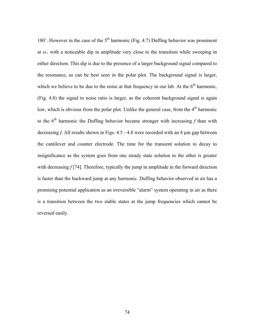
180˚. However in the case of the 5th harmonic (Fig. 4.7) Duffing behavior was prominent
at ω+ with a noticeable dip in amplitude very close to the transition while sweeping in
either direction. This dip is due to the presence of a larger background signal compared to
the resonance, as can be best seen in the polar plot. The background signal is larger,
which we believe to be due to the noise at that frequency in our lab. At the 6th harmonic,
(Fig. 4.8) the signal to noise ratio is larger, as the coherent background signal is again
low, which is obvious from the polar plot. Unlike the general case, from the 4th harmonic
to the 6th harmonic the Duffing behavior became stronger with increasing f than with
decreasing f. All results shown in Figs. 4.5 - 4.8 were recorded with an 8 μm gap between
the cantilever and counter electrode. The time for the transient solution to decay to
insignificance as the system goes from one steady state solution to the other is greater
with decreasing f [74]. Therefore, typically the jump in amplitude in the forward direction
is faster than the backward jump at any harmonic. Duffing behavior observed in air has a
promising potential application as an irreversible “alarm” system operating in air as there
is a transition between the two stable states at the jump frequencies which cannot be
reversed easily.
74
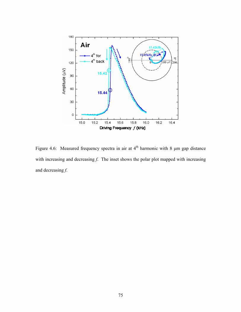
Figure 4.6: Measured frequency spectra in air at 4th harmonic with 8 μm gap distance
with increasing and decreasing f. The inset shows the polar plot mapped with increasing
and decreasing f.
75

Figure 4.7: Measured frequency spectra in air at 5th harmonic with an 8 μm gap distance
with increasing and decreasing f. The inset shows the polar plot mapped with increasing
and decreasing f. The large offset from zero of the polar plot may be due to interfering
signals at these frequencies in our lab.
76
=
Figure 4.8: Measured frequency spectra in air at 6th harmonic with an 8 μm gap distance
with increasing and decreasing f. The inset shows the polar plot mapped with increasing
and decreasing f.
(IV) Duffing behavior at 3rd to 6th harmonics at 4 μm gap distance
To study the distance dependence of the Duffing behavior we decreased the gap
distance between the cantilever and counter electrode to 4 μm, lowering Vac and Vdc to
keep the nonlinearities from increasing too much. Since decreasing the gap should
increase the nonlinearities, we expect Duffing jumps to be more prominent. The striking
77

feature with a small gap distance is that there are often two peaks in the amplitude
spectrum. Moreover, the resonance peaks taken with decreasing f spread over a broader
range from 12 to 16 kHz for all the harmonics making it difficult to read out the exact f0-
from the amplitude plot. As always at the 3rd harmonic, (Fig. 4.9) Duffing behavior was
observed more prominently with decreasing f than with increasing f at smaller gap
distance. However the Duffing-like jump with decreasing f in air is more complicated
than the results recorded with an 8 μm gap distance. The amplitude plot shows an initial
drop followed by the usual jump in the amplitude with increasing f. This dip in the
amplitude appears as a straight line in the polar plot. Data taken slower would
presumably show just a single jump, as a sufficient time at the transition frequency might
allow the transient solution to decay, and complete the jump in one frequency step. The
jump in the polar vector at f+ is smaller than at f- as might be expected for a soft spring.
The maximum amplitude dropped from 290 μV (at the 3rd harmonic) to 155 μV at
the 4th harmonic (Fig. 4.10). At the 5th and 6th harmonics the maximum amplitude
dropped to 95 μV and 8 μV respectively, which was surprisingly small as compared to 27
μV at the 6th harmonic with an 8 μm gap distance (Figs.4.11 and 4.12). At the 5th and 6th
harmonics in the frequency region ~14.5 kHz at f+ and ~ 13.8 kHz at f- there is probably
only one stable state but the instantaneous drop/jump in amplitude is so sharp that it
mimics Duffing behavior. The highlighted ‘step’ like features (Fig. 4.11) in the frequency
spectra in both directions might have potential applications such as switches or frequency
filters. Remarkable differences are identified in the amplitude and the phase during the
transition at 3rd and 4th harmonics as compared to 5th and 6th harmonics at lower gap
78

distance. This shows that the Duffing jumps are exaggerated when observed in the higher
harmonics of the driving signal. Figure 4.13 shows all the Duffing responses at different
harmonics for the 8 μm gap distance. It can be seen that the jump up frequency decreases
with increasing harmonic. If this is correct, and not due to timing lags in the lock-in, it
implies that the oscillation states of the harmonics are not locked together.
Figure 4.9: Measured frequency spectra in air at 3rd harmonic with a 4 μm gap distance
with increasing and decreasing f. The inset shows the polar plot mapped with increasing
and decreasing f.
79

Figure 4.10: Measured frequency spectra in air at 4th harmonic with a 4 μm gap distance
with increasing and decreasing f. The inset shows the polar plot mapped with increasing
and decreasing f. The double jumps are observed in both the directions for this and higher
harmonics.
80

Figure 4.11: Measured frequency spectra in air at 5th harmonic with a 4 μm gap distance
with increasing and decreasing f showing ON / OFF characteristics. The inset shows the
polar plot mapped with increasing and decreasing f. Note that large parts of the polar
plots are nearly circular arcs, and that the Duffing jumps are nearly straight lines on the
polar plots.
81

Figure 4.12: Measured frequency spectra in air at 6th harmonic with a 4 μm gap distance
with increasing and decreasing f. Inset shows the polar plot mapped with increasing and
decreasing f.
82

Figure 4.13: Measured frequency spectra in air with increasing and decreasing f at all the
harmonics with an 8 μm gap distance (Vac = 9.75 V, Vdc = 9.6 V). The arrows indicate
that the transition frequencies are different at different harmonics and the frequencies
decrease with increasing harmonics.
(V) Sensing the change in pressure using Duffing behavior
The basic principle involved in the use of Duffing oscillator for sensing
application is to first adjust the frequency to be in the bistable region where there are two
stable states at constant amplitude. In particular, when it is very close (~ 0.1 Hz) to the
83

transition frequency, a very small change in ‘any’ variable (like mass, pressure,
temperature etc.) that will make subsequent small change in frequency would cause the
amplitude (and phase) to jump up or drop down to the other stable state and can be
sensed very easily. In order to illustrate this behavior we have carried out one preliminary
experiment to show the practicality of using a Duffing cantilever for sensing. First we
pumped down the system to 5×10⁻⁵ torr using the turbo pump. Then we exposed the
system to air using a needle valve till the pressure increased to 7×10⁻⁵ torr keeping
frequency constant (the least change we could get with our setup). This caused the
resonance frequency to decrease at the 2nd harmonic, making an immediate transition to
the other state with an amplitude drop from 490 μV to 150 μV. Hence we could sense the
pressure change of 0.00002 torr at 8 μm gap distance using our Duffing resonator
(Fig.4.14). The insert in Fig. 4.14 shows the typical Duffing behavior underlying this
experiment by varying f in small (0.1 Hz) increments at 5×10⁻⁵ torr. This spectrum is
taken just before changing the pressure to 7×10⁻⁵ torr. To our knowledge, this work
represents the first experimental demonstration of sensing a pressure change using the
Duffing behavior.
84

Figure 4.14: Sensing a pressure change from 5×10⁻⁵ torr to 7×10⁻⁵ torr using the Duffing
behavior at the 2nd harmonic in the backward direction at 8 μm gap distance (Vac = 1.3 V,
Vdc = 4 V). After ~ 35 sec the pressure was increased as shown by the arrow causing the
amplitude to drop instantly from 490 μV to 150 μV. The inset shows the Duffing
behavior for this cantilever system as a function of small increments in frequency (0.1
Hz) while scanning in the backward direction at 5×10⁻⁵ torr just before changing the
pressure.
Summary
The understanding of Duffing behavior under varying conditions and parameters
provides important insights into the underlying physical mechanisms. Here we have
explored the behavior of four of the harmonics of the driving frequency (3rd through 6th)
85

using an all-electric driving and sensing method. The harmonics that we observe are due
to the nonlinearities of the cantilever, the drive system, and the sensing system. The
harmonics behave in a complicated matter that has not been studied either analytically or
computationally as yet. We observe significantly distinct features in the Duffing behavior
at different gap distances and for each of the 4 higher harmonics examined. The rich
structure of the harmonics, as illustrated in Figs 4.3 - 4.14, provides rich source of
possible applications. The essence of using the Duffing behavior is to prepare the system
with a Duffing jump not very far in frequency from the bifurcation point. One then has a
bistable system that can be used to sense small changes or store one bit. Each harmonic
has a slightly different Duffing behavior as a function of particular gap distance. Thus we
can easily create a characteristic fingerprint for any particular variable to be sensed by
tuning the different available knobs, such as the harmonics (3rd-6th), gap distances (4 μm,
8 μm) and environments (hydrogen, air and vacuum). We show one simple experiment in
which a Duffing jump is triggered by a small pressure change. The usefulness of our
Duffing system emphasizes the need for the theoretical understanding of its behavior at
the higher harmonics. Based on all the characteristic features of Duffing behavior
discussed in this chapter, it offers a wide spectrum of novel potential applications such as
band pass filters, logic gates, logic switches, alarm systems and many more yet to be
explored.
86
CHAPTER FIVE
ACTIVE SENSING IN AMBIENT CONDITIONS USING AN ELECTROSTATICALLY DRIVEN SILICON MICROCANTILEVER
Introduction
The advent of inexpensive, mass-producible and sensitive microcantilevers has
accelerated the pace of innovations in the field of physical, chemical and biological
sensing [13]. The recent developments in microfabrication technology have lead to
miniaturization, improved dynamic performance, high precision, and increased reliability.
It has been proposed that the high surface-to-volume ratio in microcantilevers (~103 m-1)
can lead to large surface forces because of the surface-molecules interactions inducing
the changes in Gibbs free energy [87]. When such interactions are restricted to one
surface, the induced differential stress causes the cantilever to bend. Changes in the
resonance frequency of the cantilever can also arise from changes in the cantilever mass
due to adsorption of the molecules. As discussed in fourth chapter, cantilevers have been
found to be useful as potential vacuum gauges, based on the damping of the surrounding
gas. [3, 66] Moreover the sensitivity and specificity of microcantilever sensors can be
enhanced by carefully optimizing the geometric design of the cantilever. For example, the
mass sensitivity of a cantilever is inversely proportional to the square root of (ρd), where
ρ is the density of the cantilever material and d is the thickness of the cantilever [13]. The
most important figures of merit for any chemical, physical or biological sensor are
response time, limit of detection (LOD), specificity, and reproducibility.
87

Although catalytic combustion, electrochemical galvanic cell, and infrared-based
detection schemes are presently in use [88], the development of a capacitive detection
based platform could definitely enhance the range of molecules that could be detected
and discriminated. In the present chapter, we employ HDR to develop a silicon
microcantilever based sensor which can be used for active sensing of gaseous species
under ambient conditions. Our sensing platform measures the changes in the mechanical
response (in amplitude and/or phase) of the vibrating cantilever in air at its resonant
frequency when exposed to several vapors and gases. We demonstrate the detection of
changes in the cantilever oscillations when exposed under ambient conditions to gases
such as, H2, D2, nitrous oxide (N2O), methane, and water vapor; and puffs of vapors of
solvents such as, hexane, benzene, methanol and isopropanol [5]. Since cantilever-based
sensors are extremely sensitive displacement sensors, they offer very little intrinsic
chemical selectivity. Hence, in this case the chemically selective layers such as polymeric
films, self-assembled monolayers, or antibody-antigen layers provide the enhanced
chemical sensitivity. Later in this chapter, we also discuss functionalized cantilevers and
show the preliminary results of detection of ammonia (NH3) and hydrogen sulphide (H2S)
using them. Finally, the response of microcantilever when exposed to vapors of different
flavors (i.e., the vapor-phase form of several beverages) illustrates this promising
approach for an easy-to-use and highly versatile sensing platform.
88

Experimental Details
All data discussed in this chapter pertain to silicon cantilever whose dimensions
are 35 µm width, 2 µm thick, and 350 µm in length. The typical experimental set up of
HDR [2] as mentioned in previous studies is slightly modified with bubbler while sensing
solvent vapors and artificial flavors (as shown in Fig. 5.1 (a)). The ac signal was swept
until the lock-in amplifier detected the f0 of the microcantilever (~ 18 kHz). All further
experiments were carried out by (i) maintaining the microcantilever near its resonant
frequency, and (ii) recording the changes in the cantilever response (change in the
amplitude ΔA and phase signals ΔΦ) during a flow of gases or vapors of polar and
nonpolar solvents (50 – 800 sccm). Gases such as, protium (H2), deuterium (D2), N2O and
CH4 were brought into the vicinity of the resonating cantilever without passing through
the bubbler in a start/stop gas flow mode with a manually controlled valve, shown in Fig.
5.1 (a) and (b). On the other hand, solvent vapors (water, hexane, benzene, methanol and
isopropanol) and several beverages (coke, diet coke, cherry coke zero, grape water,
orange juice and apple juice) were transported from the bubbler using air and hydrogen in
the case of beverages as the carrier gas. In a separate study the sensing cantilever is
functionalized to detect toxic gases like ammonia with 11-mercaptoundecanoic acid. We
coated the cantilever with a solution of (11-MUA) using a micropipette [11] only on the
side opposite to the counter electrode. In this case, the placement of counter electrode
with respect to cantilever is just opposite to that of the typical HDR set up. Hence,
counter electrode being at the top in the parallel geometry with the cantilever, the
molecule that adsorbs on the coating should cause a decrease in the amplitude of the
89

signal due to the cantilever’s bending away from the counter electrode. A 400 ppm
concentration of ammonia in helium at room pressure was introduced into the sample
chamber and three separate measurements were recorded each after five minutes.
Whereas while detecting H2S we used silicon microcantilever of the same dimensions
and coated with gold only on the side facing the counter electrode. For this experiment
we mixed the hydrogen sulphide gas with helium in the premixing chamber and diluted
this mixture even more with helium to get down to ppm concentrations.
Figure 5.1 (a): Schematic diagram of the HDR system modified for sensing gases and
solvents. The test gas is admitted in puffs without the solvent in the bubbler. For testing
solvents, the carrier gas is bubbled through the solvent, and the changes in vibration of
the cantilever are monitored.
90

Figure 5.1 (b): Digital photograph of the experimental set up illustrating the chip carrier
with cantilever and counter electrode and other electronic connections. The inset shows
the optical image of cantilever - counter electrode alignment. The test or carrier gas is
passed through ¼ ˝ tygon tubing.
Results and Discussion
Sensing of gaseous species The amplitude and phase signals for a cantilever resonating in air and exposed to
100 sccm of air bubbled through methanol, are compared in Fig. 5.2(a). The peak
amplitude increased from 150 μV in ambient air to 170 μV in methanol. Likewise, the
phase signal in air which resembles that of a damped SHO, is also sensitive to the
91

environment around the microcantilever and it decreased upon exposure to methanol.
Once we determine f0 using the phase and peak amplitude, we set the lock - in amplifier
very close to f0 to detect the ΔA and ΔΦ induced by change in the environment in the
vicinity of the cantilever. ΔΦ is defined as ΦA – ΦΜ, where ΦA and ΦΜ correspond
respectively to the magnitude of phase change in air and methanol (see Fig. 5.2(a)). Thus,
ΔA and ΔФ signals can serve as sensitive indicators for the presence or absence of
specific gases near the resonating cantilever. In Fig. 5.2(b), we plot ΔA and ΔФ for a
microcantilever resonating in air and when intermittently exposed to 100 sccm of
methanol. The amplitude increases and the phase decreases every time a pulse of the air
with methanol is admitted. The response returns to the base line representing the
amplitude and phase in ambient air promptly between puffs. The exposure time for each
puff was about 30 seconds. While ΔA increased by ~ 6 μV, ΔФ decreased by ~ 50,
indicating a slight decrease in f0. The greater increase observed in peak amplitude (~ 20
μV) in Fig. 5.2(a) as compared to the increase in ΔA (~ 6 μV) seen in Fig. 5.2(b) can be
attributed to the greater exposure time in the former case as the cantilever is continuously
exposed to methanol vapors than the latter.
92
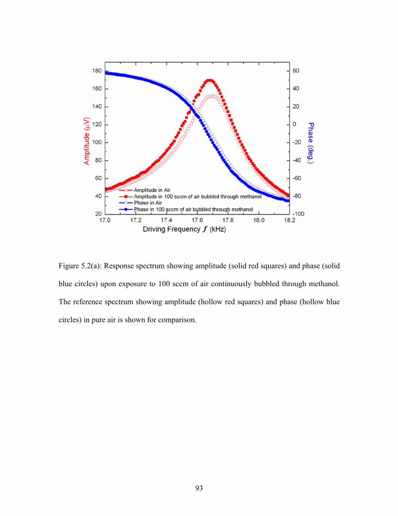
Figure 5.2(a): Response spectrum showing amplitude (solid red squares) and phase (solid
blue circles) upon exposure to 100 sccm of air continuously bubbled through methanol.
The reference spectrum showing amplitude (hollow red squares) and phase (hollow blue
circles) in pure air is shown for comparison.
93

Figure 5.2(b): Response of the cantilever at the selected f0 = 17.69 kHz showing the ΔA
(solid red squares) and ΔΦ (solid blue circles) upon exposure to puffs of 100 sccm of air
bubbled through methanol.
In general, we observed that when the cantilever is exposed to the vapors of any
solvent, the phase always decreases, implying that f0 always decreases. But the amplitude
response is a function of both the change in maximum peak amplitude at resonance and
the value of f0, and can depend upon the selection of the frequency manually entered into
the lock-in amplifier, which might be quite close to f0 but not accurate. Since the
derivative of the amplitude with respect to frequency at the selected frequency changes
sign at the actual f0, the amplitude response can go up or down for the same change in f0
94

depending upon whether the selected frequency is slightly lower or slightly higher than
the actual f0 (see Figs. 5.4(a) and 5.4(b)). But the derivative of the phase with respect to
the selected f0 is nearly constant near resonance. Thus the direction and magnitude of the
phase change will always closely indicate the direction and magnitude of the change in f0.
This in turn is determined by the gas cantilever interactions, irrespective of the selection
of f0. Hence it is advisable not to depend on only ΔA but to take into account both ΔA and
ΔФ while sensing gases and solvents. For example, in the case of methane, there is a
large increase in amplitude but only a small change in phase and thus in f0 (see Fig.
5.3(a)). The ΔA increased by ~ 14 μV and ΔФ increased by ~ 30 when exposed to 100
sccm of methane as seen in Fig. 5.3(b). But when exposed to 100 sccm of nitrous oxide,
surprisingly the amplitude increased by ~ 10 μV but the phase and f0 both decreased as
shown in Fig. 5.4(a). Hence the ΔФ increase of +30 for methane as opposed to the ΔФ
drop of -90 (Fig. 5.4(b)) for nitrous oxide shows that methane causes an increase in f0
whereas nitrous oxide causes a decrease in f0. This can be attributed to the fact that
methane has a lower molecular mass and nitrous oxide has a higher molecular mass than
air [3].
95

Figure 5.3(a): Response spectrum showing amplitude (solid red squares) and phase (solid
blue circles) upon exposure to 100 sccm of methane (CH4). The spectrum showing
amplitude (hollow red squares) and phase (hollow blue circles) in air is shown for
reference. ΔA is positive for all choices of selected f0 with very small change in f0 and a ~
15% change in the peak amplitude. The corresponding ΔA and ΔΦ plots are shown in
Fig. 5.3(b).
96
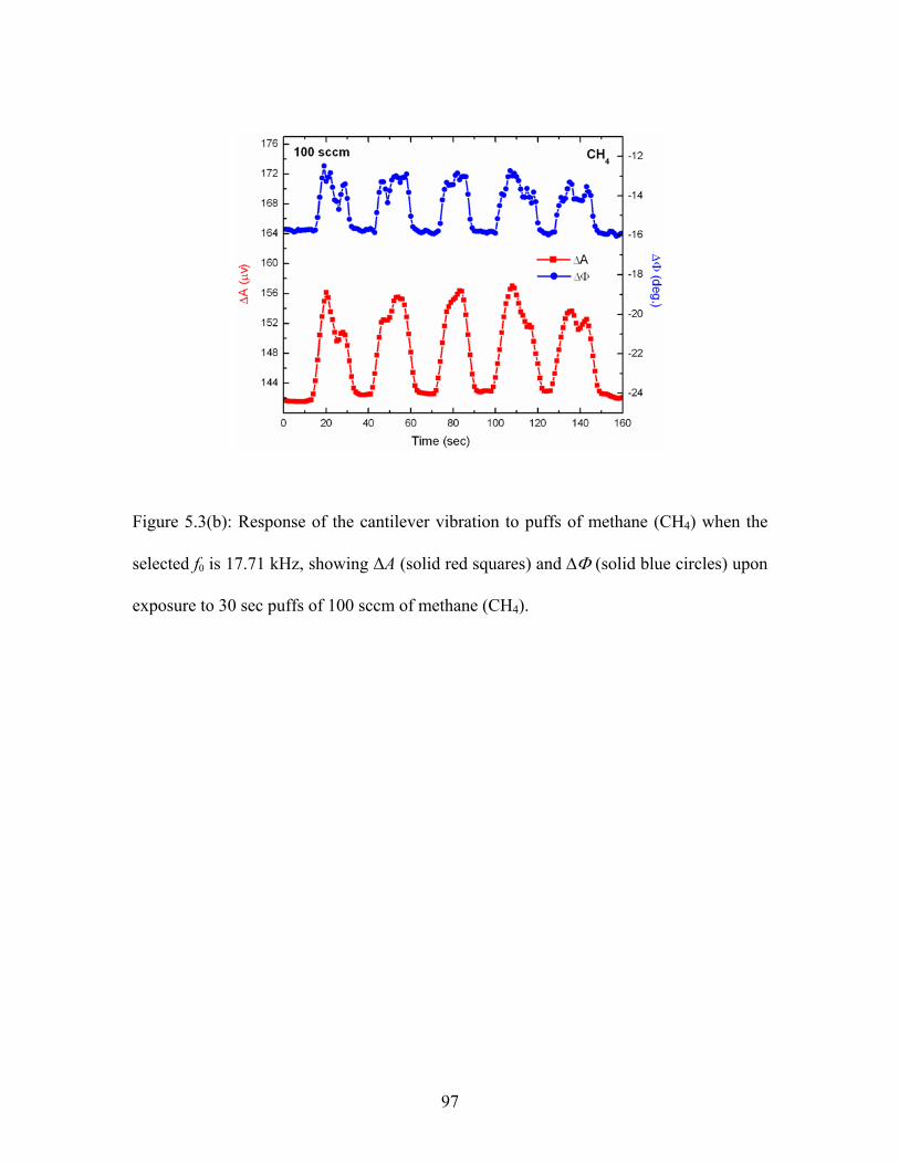
Figure 5.3(b): Response of the cantilever vibration to puffs of methane (CH4) when the
selected f0 is 17.71 kHz, showing ΔA (solid red squares) and ΔΦ (solid blue circles) upon
exposure to 30 sec puffs of 100 sccm of methane (CH4).
97

Figure 5.4(a): Response spectrum showing amplitude (solid red squares) and phase (solid
blue circles) upon exposure to 100 sccm of nitrous oxide (N2O). The spectrum showing
amplitude (hollow red squares) and phase (hollow blue circles) in air is shown for the
reference. With a 10% decrease in peak amplitude and a ~100 change in f0, ΔA can be
positive or negative depending on the f0 selected. If the selected f0 is 17.7 kHz, there will
be increase in the amplitude and ΔA will be positive whereas if the selected f0 is 17.9
kHz, there will be decrease in the amplitude and ΔA will be negative (as shown by the red
arrows). But the ΔΦ will always be negative as shown by the blue arrow irrespective of
the selected f0.
98

Figure 5.4(b): Response at a selected frequency of 17.7 kHz, showing ΔA (solid red
squares) and ΔΦ (solid blue circles) upon exposure to 100 sccm puffs of nitrous oxide
(N2O).
In Figs. 5.5(a) and 5.5(c), we plot the amplitude and phase responses for a
microcantilever resonating in air and when intermittently exposed to 100 sccm of H2 and
D2 gases, respectively. ΔA increases every time when exposed to H2 as does ΔΦ. The
increase in amplitude signal for D2 is almost half of that for H2, but there is not much
change in the phase and f0 for either of gas as seen in Figs. 5.5(a) and 5.5(c). It is very
unlikely that the observed change in amplitude is due to physisorption of H2 or D2
molecules, or due to the influence of their dielectric properties. The observed increase in
99

amplitude can be due to the changes in the damping factor. At this pressure, the damping
γ is inversely proportional to the square root of the atomic mass m [60], so that
∆γ/γ ≈ -½∆m/m (6.1)
Approximating m for air as 30, ∆m for protium is 28 and for deuterium is 26, implying
that the effect on damping due to a small amount of H2 added to air is about the same as
D2, consistent with our experiment. The ΔA and ΔФ exhibit similar trends in case of H2
and D2 such as, ΔA increased by ~ 8 μV and ΔФ increased by ~ 40 (Figs. 5.5(b) and
5.5(d)). Hence in order to differentiate between H2 and D2, we reduced the gap distance
between the gas inlet and the microcantilever which might lead to more gas -cantilever
interactions. As seen in Fig. 5.5(e), now even the ΔA for H2 (m = 2) is roughly twice as
that for D2 (m = 4) which illustrates that we can successfully distinguish between the
isotopes of hydrogen based on change in the mass. The inset in this figure helps to
explain the kind of response observed during this particular experiment.
100

Figure 5.5(a): Response spectrum showing amplitude (solid red squares) and phase (solid
blue circles) upon exposure to 100 sccm of protium (H2). The spectrum showing
amplitude (hollow red squares) and phase (hollow blue circles) in air is shown for
reference.
101

Figure 5.5(b): ΔA (solid red squares) and ΔΦ (solid blue circles) upon exposure to puffs
of 100 sccm of protium (H2) at 17.71 kHz. ΔA increases every time when exposed to H2
as does ΔΦ. Both return to the base lines representing the amplitude and phase in
ambient air promptly.
102

Figure 5.5(c): Response spectrum showing amplitude (solid red squares) and phase (solid
blue circles) upon exposure to 100 sccm of deuterium (D2). The spectrum showing
amplitude (hollow red squares) and phase (hollow blue circles) in air is shown for the
reference.
103

Figure 5.5(d): Response of ΔA (solid red squares) and ΔΦ (solid blue circles) upon
exposure to 100 sccm of deuterium (D2) when the selected f0 = 17.71 kHz. ΔA increases
every time when exposed to D2 with a concomitant increase in ΔΦ. The responses
promptly return to the base lines representing the amplitude and phase in ambient air.
104
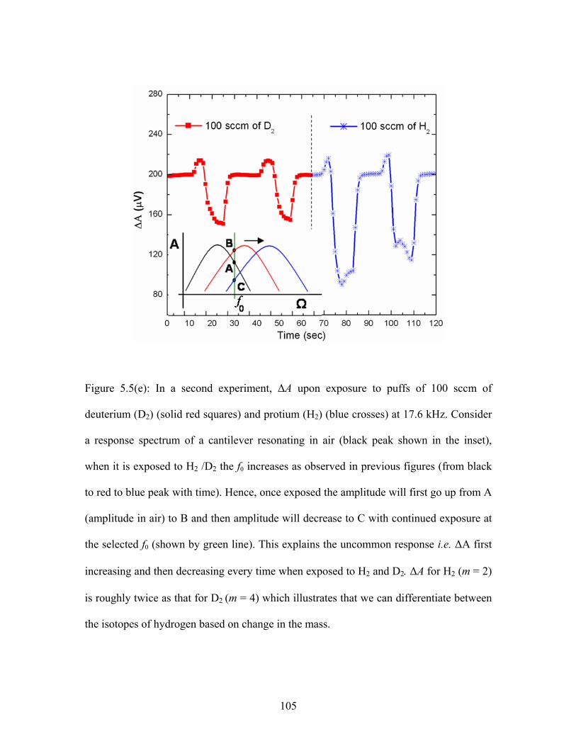
Figure 5.5(e): In a second experiment, ΔA upon exposure to puffs of 100 sccm of
deuterium (D2) (solid red squares) and protium (H2) (blue crosses) at 17.6 kHz. Consider
a response spectrum of a cantilever resonating in air (black peak shown in the inset),
when it is exposed to H2 /D2 the f0 increases as observed in previous figures (from black
to red to blue peak with time). Hence, once exposed the amplitude will first go up from A
(amplitude in air) to B and then amplitude will decrease to C with continued exposure at
the selected f0 (shown by green line). This explains the uncommon response i.e. ΔA first
increasing and then decreasing every time when exposed to H2 and D2. ΔA for H2 (m = 2)
is roughly twice as that for D2 (m = 4) which illustrates that we can differentiate between
the isotopes of hydrogen based on change in the mass.
105

One would expect the amplitude to decrease in presence of nitrous oxide, since it
has a higher ‘m’ than air, but the opposite response is observed (Fig. 5.4(a)). It is difficult
to predict the response of the cantilever when exposed to a particular gas/vapor as we
can’t quantify the exact amount of gas coming in contact with the cantilever. Thus the
effect of the gas on the cantilever depends not only on the interaction of the gas with the
cantilever, but also on our ability to deliver the gas to the cantilever. In fact, in our
experimental set up we try to sense puffs of the test gas/vapor. Hence we propose that a
gas lighter than air will go up easily without much interaction with the cantilever whereas
a heavier gas will spend more time near the cantilever affecting its response to a greater
extent. For example, ΔA increases by ~14 μV in presence of methane compared to ~ 8 μV
for protium (Figs. 5.3(b) and 5.5(b)). Next we focus on the ΔA and ΔФ changes induced
due to various concentrations of H2. The response showed an increase in both ΔA and ΔФ
which increased monotonically as the protium flow was increased from 50 sccm to 800
sccm (Fig. 5.6). The inset shows a typical amplitude response for the microcantilever
when exposed to various amounts from 50 sccm to 800 sccm of protium in a start/stop
gas flow mode. As expected, larger flow rates give larger changes. In chapter 3 [4] we
have already shown that nearly pure protium, helium, air and argon gas atmospheres in a
closed chamber have large effects on the damping, proportional to the inverse square root
of the molecular mass of the gas. However, in this chapter the concentrations of the test
gas are never large enough to allow this kind of discrimination.
106

Figure 5.6: Dependence of ΔΑ and ΔΦ (measured at the selected frequency f0 = 17.71
kHz) on the amount concentration of protium (H2) molecules present in the vicinity of the
cantilever. The inset shows the response spectra upon exposure to puffs of increasing
concentration of protium from 50 to 800 sccm. The base line represents the amplitude in
ambient air.
Sensing of solvent vapors The sensing of various polar and non polar solvents (n-hexane, benzene,
methanol, iso-propanol and water) showed an increase in amplitude (Fig. 5.7(a)) and
decrease in phase (not shown) upon exposure to 100 sccm of air bubbled through all
these solvents. It shows that the normalized amplitude ∆A/A is highest for n-hexane and
decreases uniformly with decreasing molecular mass of the solvent vapors under study.
107

The vapor pressures at room temperature for water, iso- propanol, methanol, benzene and
n-hexane are 15, 44, 128, 100 and 127 mm of Hg respectively. Hence due to the lower
vapor pressures for water and iso-propanol we get very small response in terms of the
changes in amplitude for these two solvents as seen in Fig. 5.7(a). The peculiar trends
observed in the normalized amplitude responses of these solvents are correlated to their
different dependences on mass, dielectric constant and polarity index (see Fig. 5.7(b)). In
general, the normalized amplitude showed a decreasing trend with increase in polarity
index, dielectric constant and inverse of mass. Although it was not possible to determine
exactly which property determined the result, the previous study would favor the
molecular mass of the solvent as the dominant characteristic. As opposed to solvent
vapors, while sensing gases, the normalized amplitude decreased with increase in
molecular mass of the gas as expected except for methane for reasons we do not
understand (as seen in Fig. 5.8).
108

Figure 5.7(a): Normalized amplitude changes upon exposure of the cantilever vibrating
near f0 to 100 sccm of air bubbled through water, iso-propanol, methanol, benzene and n-
hexane. The numbers on the left axis indicate ΔA/A for each individual solvent vapor.
109

Figure 5.7(b): The normalized amplitude ∆A/A for the solvents methanol, water, iso-
propanol, benzene and n-hexane plotted as a function of three normalized parameters: the
inverse of mass, dielectric constant and polarity index. The normalization of each
parameter consisted of dividing the value of that parameter for each solvent by the
maximum value of the parameter in this set of solvents. The lines are only guides to the
eye. Methanol may interact differently than the other solvents.
110
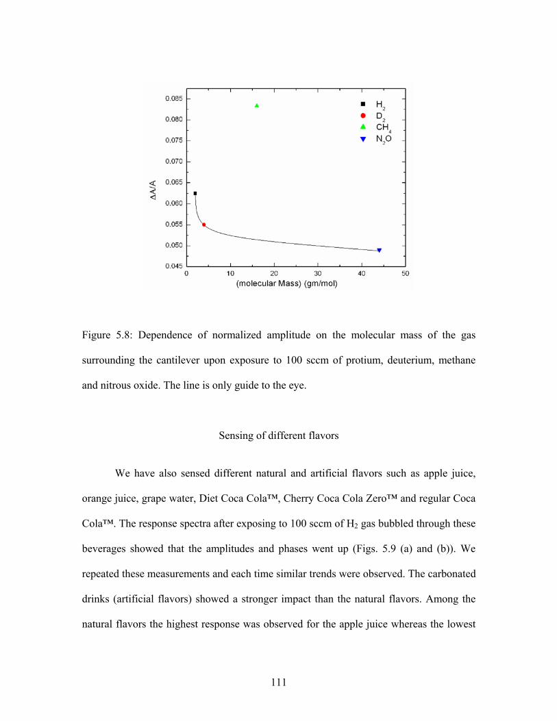
Figure 5.8: Dependence of normalized amplitude on the molecular mass of the gas
surrounding the cantilever upon exposure to 100 sccm of protium, deuterium, methane
and nitrous oxide. The line is only guide to the eye.
Sensing of different flavors We have also sensed different natural and artificial flavors such as apple juice,
orange juice, grape water, Diet Coca Cola™, Cherry Coca Cola Zero™ and regular Coca
Cola™. The response spectra after exposing to 100 sccm of H2 gas bubbled through these
beverages showed that the amplitudes and phases went up (Figs. 5.9 (a) and (b)). We
repeated these measurements and each time similar trends were observed. The carbonated
drinks (artificial flavors) showed a stronger impact than the natural flavors. Among the
natural flavors the highest response was observed for the apple juice whereas the lowest
111

one was the orange juice. The successful separation among the Diet Coca Cola™, regular
Coca Cola™ and Cherry Coca Cola Zero™ was an interesting outcome of our highly
sensitive non-functionized microcantilever sensor. It displayed characteristic responses
for these natural and artificial flavors.
Figure 5.9 (a): Response spectra comparing amplitudes upon exposure to 100 sccm of
hydrogen bubbled through different flavors such as grape water, orange juice, Diet Coca
Cola™, regular Coca Cola™, Cherry Coca Cola Zero™ and apple juice. The baseline
represents the amplitude in ambient air.
112

Figure 5.9 (b): Response spectra comparing phases upon exposure to 100 sccm of
hydrogen bubbled through different flavors such as grape water, orange juice, Diet Coca
Cola™, regular Coca Cola™, Cherry Coca Cola Zero™ and apple juice. The base line
represents the phase in ambient air.
Sensing of toxic gases The silicon microcantilever of the same dimension was coated with 11-
mercaptoundecanoic acid in order to detect toxic ammonia gas. Ammonia can be detected
as it forms reversible hydrogen bonds with the acidic tail of the 11-MUA [11]. Figure
5.10 (a) compares the resonant frequency of the cantilever before and after it was
functionalized. It shows a distinct upshift in the resonant frequency from 21.8 kHz to
113

22.7 kHz, which could be attributed to the stiffening of the cantilever after coating and
the amplitude, was damped. Under ideal conditions (immersion of the cantilever in 11-
MUA solution for over 10 hours), the sulfur end of the molecules will bind to the gold
surface, and the molecules self-assemble perpendicular to it. With our present
configuration of chip, immersion of the cantilever was not possible, and so the 11-MUA
solution was simply placed dropwise onto it and allowed to evaporate. Though the sulfur-
gold bonds formed quickly within this time, a well-organized monolayer did not have
time to self-assemble before evaporation. Thus, the molecular organization of the
cantilever coating is not uniform, resulting in fewer binding sites for the ammonia per
unit area. Three separate measurements recorded after exposure to 400 ppm of ammonia
in helium show 7.0, 7.3, and 10.3 % decrease in the signal amplitude, respectively (Fig.
5.10 (b)), demonstrating the reproducible detection of the binding of ammonia. Between
measurements, the chamber was flushed with helium, and the signal amplitude increased
to its former intensity, showing the reversible nature of the ammonia binding. While both
the detection limit and response are less than ideal, this rough experiment demonstrates
the first proof of principle of sensing a gas via electrostatic detection of cantilever
resonance using HDR.
114
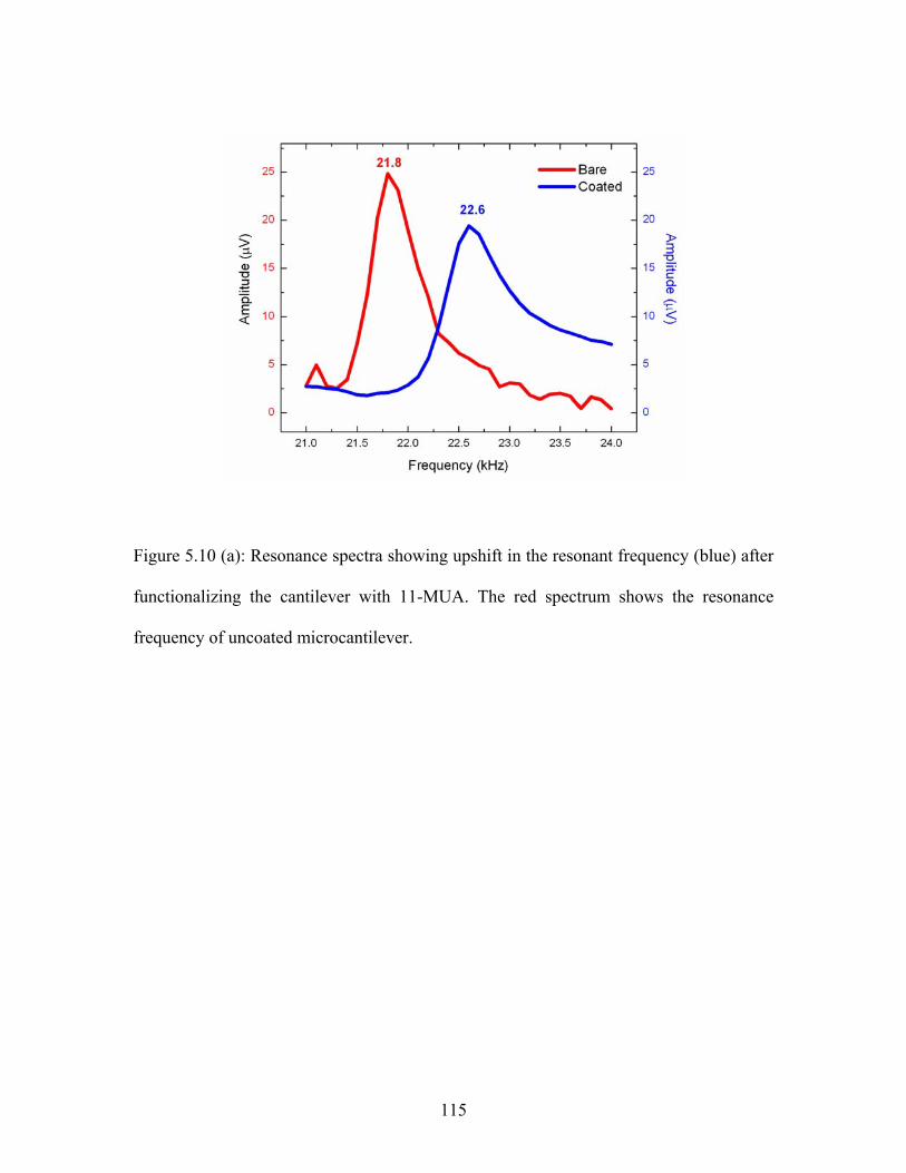
Figure 5.10 (a): Resonance spectra showing upshift in the resonant frequency (blue) after
functionalizing the cantilever with 11-MUA. The red spectrum shows the resonance
frequency of uncoated microcantilever.
115

Figure 5.10 (b): Three separate measurements showing the change in amplitude when
exposed to 400 ppm of ammonia in helium (solid blue circles). The amplitude in pure
helium environment (solid red circles) dropped by 7.0, 7.3, and 10.3 % respectively, in
presence of ammonia in these measurements.
When exposed to various amounts of H2S, we noticed a monotonic rise in the size
of signal with increase in the concentration of hydrogen sulphide gas in helium from 0 to
100 ppm in the chamber (Fig. 5.11). The sulphur-gold affinity causes the cantilever to
bend towards the counter electrode leading to greater signal with higher concentrations.
There is not only change in resonant frequency as we go from pure helium to helium
mixed with hydrogen sulphide but we also observed the change in the amplitude of
signal. The complete saturation of gold coated cantilever with sulphur led to the highest
116

amplitude and increase in the resonant frequency. The validity of this behavior is checked
by repeating the experiment with the same cantilever.
Figure 5.11: The ΔA signal increases monotonically with the increase in the concentration
of hydrogen sulphide gas in helium from 0 to 100 ppm in the chamber. A concomitant
downshift in f0 from 18.23 kHz (at 0 ppm) to 18.10 kHz (at 100 ppm) was observed.
Conclusions We have demonstrated qualitative sensing of different gases and solvent vapors.
This sensor platform features a reasonable selectivity and rapid response. It is clear from
117

the above experiments, that any chemical specie carries a particular ‘fingerprint’ while
using HDR based on the criteria that involve 1) the static (dielectric effects) and dynamic
capacitance between the cantilever and counter electrode, 2) the detection of trace
amounts of adsorbed molecules through a shift in the resonant frequency, 3) variations in
the environment which affect the mechanical damping of the microcantilever. At present
the exact mechanisms of these responses are not fully understood and further
investigation is in progress. Most of these measurements are promising approaches to a
completely new class of easy to use miniaturized sensor systems. The functionalized
sensor has potential applications in the area of selective detection of multielement/
multicomponent systems. Further development would involve optimizing the geometry
and configuration of the cantilever and counter electrode, functionalizing the cantilever to
suit the gas(es) to be detected, and improving the electronics.
The functionalized cantilevers showed different responses when exposed to
ammonia and hydrogen sulphide. This may be due to: (i) Our method depends on the
oscillator non-linearities. A small change in the gap distance can have a large effect on
the non-linearities and hence the amplitude at the 2nd harmonic which we measure. (ii)
The energy involved in a cantilever’s motion is equal to ½ kA2 (= ½ mf02A2) in SHO
which remains constant. Hence, if the resonant frequency increases due to stiffening of
cantilever as in case of ammonia, it decreases the amplitude. For hydrogen sulphide, the
amplitude went up causing the resonant frequency to downshift as f0A is constant.
118

CHAPTER SIX
DETERMINATION OF CARBON NANOTUBE DENSITY BY GRADIENT SEDIMENTATION
Introduction
As discussed earlier, in chapters 2 and 3 HDR is a versatile technique and it can
used to determine the mechanical properties such as Young’s modulus of silicon
microcantilever using equation (2.27),
2 4
2
( )( )
i
i y
A f lEI
ρβ
= (2.27)
Hence, if we can measure the resonant frequency (f0) of micro- or nanocantilevers
using HDR and determine their densities (ρ), then we can calculate their respective
Young’s modulus. In order to demonstrate the feasibility of using HDR at the nanoscale,
we have driven individual multi-walled carbon nanotube (MWNT) into resonance and
determined its Young’s modulus. However, MWNTs grow with a dominant inner/outer
diameters and length, depending on the growth parameters used in the experiment.
Therefore, accurate knowledge of the MWNT density is essential in the determination of
its Young modulus. In this chapter, a gradient sedimentation technique[89] is described
which provides densities for MWNTs and single walled carbon nanotubes (SWNTs) that
agree very well with respected computed densities.
Carbon nanotubes (CNTs) have revolutionized the scientific community with
fundamentally interesting properties and potential for numerous applications owing to
their unique electrical, optical, thermal, and mechanical properties [90-93]. Surprisingly,
119
a fundamental physical property, viz. the density of CNTs, has received relatively little
attention. Since density is directly associated with the intrinsic structure of the CNT, it
can be used to quantify its purity after separation from the as-prepared soot. Moreover,
since the presence of defects alters the structure of a CNT, the density may also serve as a
measure of the quality of the CNTs.
A SWNT can be formed by folding a single graphene sheet into a seamless tube
with a diameter of ~1 nm. The most important synthesize techniques for SWNTs are
pulsed laser vaporization, chemical vapor deposition and electric arc discharge.
Depending upon how the grapheme sheet is rolled into a SWNT, there are three classes of
SWNTs with different chiralities, viz. armchair, zigzag, and chiral nanotubes [90]. The
unit cell of an individual SWNT is dictated by its chirality leading to different lattice
parameters and densities. Simulations by Gao et al. [94] verified this dependence
showing that the (10,10) armchair tubes possess a lattice parameter of a (10,10) = 16.78 Å
and a density of ρ (10,10) = 1.33 g/cm3. The corresponding values for a (17,0) zigzag tube
are a (17,0) = 16.52 Å and ρ (17,0) = 1.34 g/cm3, and a (12,6) = 16.52 Å and ρ (12,6) = 1.40
g/cm3 for a chiral (12,6) tube. A MWNT is formed when several SWNTs with increasing
tube diameters self-assemble concentrically into a single carbon nanotube [90]. For a
typical MWNT with an outer diameter of 8-15 nm and an inside diameter of 3-5 nm, the
density is reported to be around 2.1 g/cm3 [95].
The density gradient sedimentation method is widely used for measuring the
densities or molecular weights of macromolecules, as well as for separating colloids and
minerals. In this method, a sodium metatungstate-water solution is centrifuged to form a
120

density gradient in the centrifugal field. The macromolecule sediments to a position in the
gradient where its density closely matches with the density of the solution. This technique
can separate macromolecules with remarkably small differences in density. With this
technique, in a standard centrifuge cell at 40 000 rpm using cesium chloride gradient
solution, a density difference of 0.014 g/cm3 in macromolecules results in a well defined
band spanning ~0.5 mm which strongly emphasizes its high resolution capability [89].
For this study, the sodium metatungstate (Na6[H2W12O40], abbreviated as NamW)
solution was selected to determine the densities of CNTs because of NamW’s high
density (3.12 g/cm3 at 25 °C), low viscosity at high concentration, and high solubility in
water [89]. For samples available in small amounts or low concentrations, this technique
is more convenient and accurate than other conventional techniques [96].
Experimental Procedure
Gradient Centrifugation: NamW-water solution was prepared by adding NamW
(2.82 g/mL, Acros Organics) to the distilled water at a volume ratio of 7: 9 (NamW/H2O)
[97]. CNTs (~ 0.5 mg) were added to 3 mL of NamW-water solution in a Beckman
polyallomer centrifuge tube (11mm × 60 mm). Centrifugation was performed with a
Beckman SW56 rotor at 23 000 rpm and 20 °C. After 60 hr of centrifugation, well-
defined bands were formed and their distances from the meniscus were measured. The
gradients were fractionated in 200-μL fractions, and each fraction was weighed on a
Mettler H20T balance.
121

Carbon Nanotube Samples: The pristine SWNT (p-SWNT) bundles and isolated
SWNTs (iso-SWNT) used in this study were synthesized by the electric arc discharge and
chemical vapor deposition (CVD) methods, respectively [1]. The ultrasonic agitation of
pristine SWNTs in a 3:1 mixture of concentrated H2SO4 and HNO3 resulted into acid-
treated SWNTs (acid-SWNT). This acid treatment makes SWNTs soluble in water with
abundant carboxyl end-groups formed at defect sites and terminals [98]. MWNTs were
synthesized using two methods: (i) a thermal decomposition of a ferrocene-xylene
mixture [99] and (ii) by striking an electrical arc discharge between two graphite
electrodes in an inert Ar atmosphere [100]. All these CNTs samples were characterized
after sedimentation by transmission electron microscopy (TEM) and micro-Raman
spectroscopy. Fractionated CNT samples were stained with uranyl acetate and deposited
on 300-mesh copper grids for TEM characterization with a Hitachi 7600 microscope. The
micro-Raman data for SWNTs was gathered using a TRIAX 550 single-grating
spectrometer (groove density 1200 grooves/mm) equipped with a liquid nitrogen-cooled
charge-coupled device (CCD). An Ar ion laser with a wavelength of 514.5 nm was used
to excite Raman scattering from the CNTs using 50 × objective of a Leica microscope.
Results and discussion After centrifugation, the well-defined bands formed corresponding to each of the
CNT structures are shown in Figure 6.1. The different structures sedimented at different
levels in gradients prepared under identical conditions (see Fig. 6.1).
122

Micro-Raman Spectroscopy The various bands seen in Fig.6.1 were confirmed to contain MWNTs, p-SWNT
bundles, or iso-SWNTs using micro-Raman spectroscopy as demonstrated in Figure 6.2.
The micro-Raman spectrum of iso-SWNTs (shown in green), show the signature radial
breathing modes (RBM) at 157 and 266 cm-1 implying SWNT diameters of 1.58 and 0.93
nm respectively at room temperature. The nanotube diameters were estimated using the
empirical relation,
248/t RBMd ω= ,
where dt and ωRBM refer to the tube diameter and the RBM mode angular frequency [101].
The peaks present at ~520 and ~950 cm-1 correspond to the Raman modes of the Si
substrate The tangential (G) band is observed at 1588 cm-1 with disorder induced band
(D-band) of negligible intensity [90]. Lorentzian lineshape of the RBM in the Raman
spectra suggested that the SWNTs are isolated. In the Raman spectrum of arc-prepared
MWNTs, a pronounced D-band is also observed at 1357 cm-1 in addition to the G-band at
1581 cm-1. However, p-SWNT bundles show the RBM and G-bands at 170 and 1588 cm-
1, respectively. The lineshape of the G-band in each spectrum of pristine SWNTs hints
that the 514.5 nm excitation couples to isolated semiconducting SWNTs [102].
Figure 6.3 shows the density profile along the length of a NamW gradient. The
density data, obtained by weighing each gradient fraction of 200 μL, show the linear
dependence on the distance of the gradients from the meniscus. The solid circle on the
straight line indicates the position of the sharp band formed by the p-SWNT bundles (see
123

Figure 6.1b). The density corresponding to this position from the meniscus in the gradient
is 1.90 g/cm3. The densities of other forms of SWNTs and MWNTs were calculated using
a similar approach and are presented in Table 6.1. The experimental deviation was
calculated for the enlisted densities in Table 6. 1 using three independent experiments as,
( )( )
2
1nρ ρ−
−∑
where ρ is the density measured for each experiment, ρ is the mean density, and n = 3.
Figure 6.1: Various structures of CNTs, including (a) acid-SWNT, (b) p-SWNT, (c)
MWNT and (d) iso-SWNT, form bands at different levels in gradients prepared and run
identically.
124

acid-SWNT p-SWNT iso-SWNT MWNT (CVD)
MWNT (Arc Discharge)
density (g/cm3) 1.74 ± 0.04 1.87 ± 0.03 2.13 ± 0.04 2.09 ± 0.02 2.11 ± 0.03
Table 6.1: The measured densities of various structures of CNTs. The data represent
means of three independent experiments and the numbers following “±” are standard
deviation.
Figure 6.2: Raman characterization of MWNTs, p-SWNTs and iso-SWNTs. The two
peaks in the spectrum of iso-SWNTs marked by “Si” were from silicon substrate.
125

-10 0 10 20 30 40 500.8
1.0
1.2
1.4
1.6
1.8
2.0
2.2
2.4
2.6D
ensi
ty (g
/cm
3 )
Distance to meniscus (mm)
Figure 6.3: The density profile along the length of a gradient obtained from p-SWNTs.
The density data, obtained by weighing each gradient fraction of 200 μL, fit a straight
line y = 0.2903x + 1.0371, where x is the distance from the meniscus to a particular
fraction and y is its density. The solid circle on the trendline of the density gradient
indicates the position of a sharp band corresponding to p-SWNTs. The density of this
point in the gradient is 1.90 g/cm3.
Transmission Electron Microscopy (TEM) Extensive TEM studies were conducted to determine (i) diameter distribution of
individual SWNTs within a p-SWNT bundle, (ii) distribution of p-SWNT bundle
diameters, and (iii) distribution of MWNT diameters (Figure 6.4). From Gaussian
analysis of the histograms shown in Figure 6.4, the mean diameters of individual tubes in
126

p-SWNT bundles, p-SWNT bundles, and of MWNTs were determined to be 1.44 ± 0.04,
8.00 ± 0.11, and 49.26 ± 2.16 nm, respectively.
127
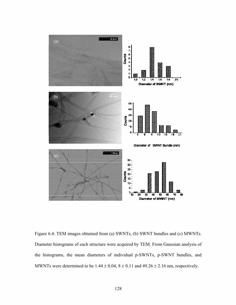
Figure 6.4: TEM images obtained from (a) SWNTs, (b) SWNT bundles and (c) MWNTs.
Diameter histograms of each structure were acquired by TEM. From Gaussian analysis of
the histograms, the mean diameters of individual p-SWNTs, p-SWNT bundles, and
MWNTs were determined to be 1.44 ± 0.04, 8 ± 0.11 and 49.26 ± 2.16 nm, respectively.
128

Theoretical Model
The experimentally determined diameters were used in the model described
further to estimate the densities of p-SWNT bundles and MWNTs. The density of an
individual SWNT was computed by considering it as a rolled honeycomb sheet of length
L and diameter DSWNT. Density ρSWNT is given as
2 22 2 2
2
4
4 4
SWNT
C CSWNT
SWNT SWNT SWNT
D LN m D Dm Zu
D DV DL L
πρ
π π= = = =
ZuD
(6.1)
where Nc and mc correspond to the number and mass of the carbon atoms. In equation
(6.1), D2 = 2.83 Å is the longest distance between carbon atoms in a single hexagonal
lattice [90], Z is the atomic mass for carbon atom and u is the atomic mass unit
(1.6605×10⁻²⁷ kg). Following a similar rationale the density of a SWNT bundle can be
written as:
2 22 2 2 2
2
4
4 4
SWNTSWNT
SWNT C C SWNT SWNTBundle
Bundle Bundle Bundle
D Lnn N m n D ZD Dm Zu
D DV DL L
πρ
π π= = = =
uD
(6.2)
where DBundle is the bundle diameter which can be expressed as:
( ) iltiertierSWNTBundle DnnDD 212 ++= (6.3)
nSWNT = 1, 7, 19, 37, 61 is the number of SWNTs in each tier and ntier is the number of tiers
for each bundle, and Dil = 3.38 Å is interlayer spacing shown in Fig. 6.5(a) [90].
129
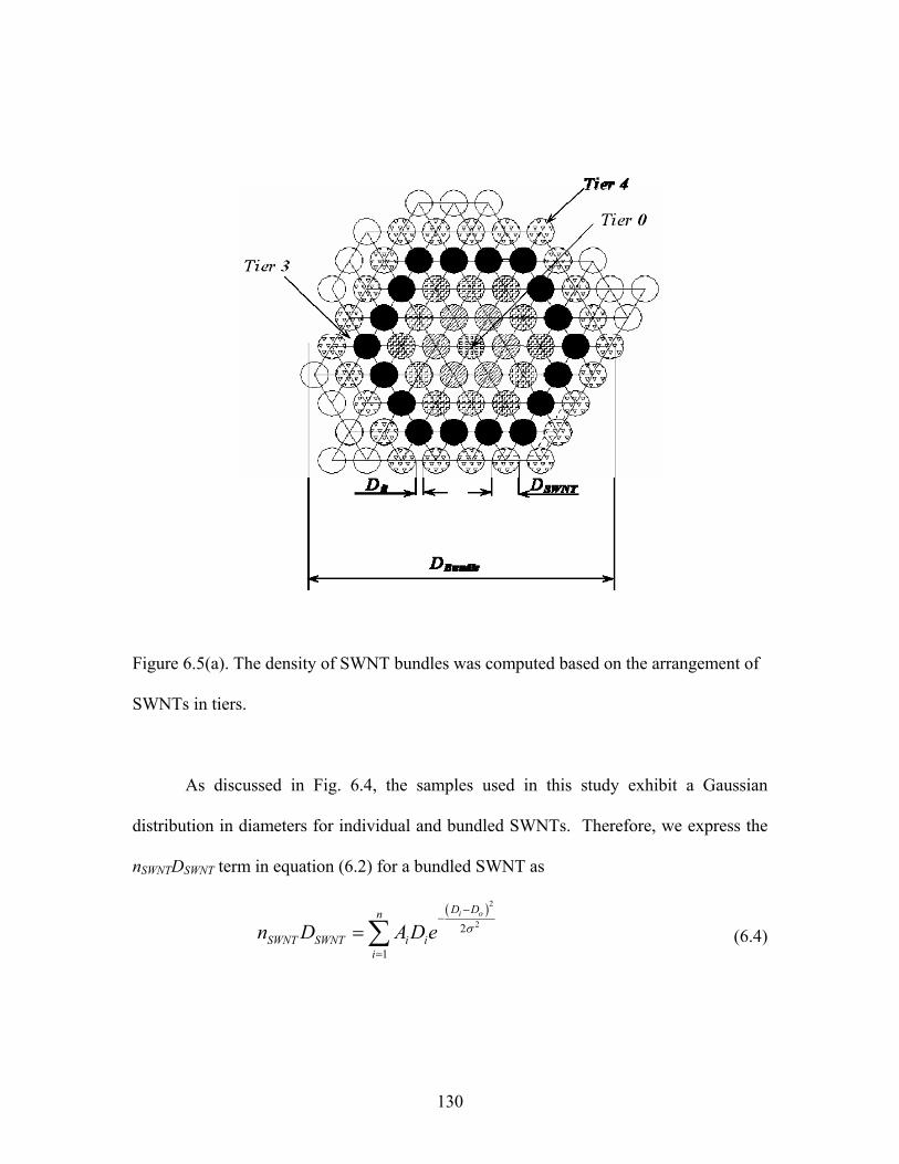
Figure 6.5(a). The density of SWNT bundles was computed based on the arrangement of
SWNTs in tiers.
As discussed in Fig. 6.4, the samples used in this study exhibit a Gaussian
distribution in diameters for individual and bundled SWNTs. Therefore, we express the
nSWNTDSWNT term in equation (6.2) for a bundled SWNT as
( )2
22
1
i oD Dn
SWNT SWNT i ii
n D A D e σ−
−
=
= ∑ (6.4)
130

where Ai, Di, Do, and σ are obtained from a Gaussian fit to the experimental diameter
distribution of individual SWNT within a bundle (see Fig. 6.4) [102]. Ai, Di, Do and σ
correspond to the weighting factor, binning diameter, median diameter and the standard
deviation, respectively. Substituting equations (6.3) and (6.4) in equation (6.2) gives
( )2
222 2
12
4 i oD Dn
Bundle i iiBundle
Zu A D eD D
σρ−
−
=
= ∑ (6.5)
It is a well known fact that residual catalysts are present in pristine SWNTs. Next we
discuss our model calculations taking into account the presence of catalyst particles. We
consider the measured density of SWNT bundles (ρmeasured) in terms of the density and
volume of bundled SWNTs and catalyst particles as follows:
⎟⎟⎠
⎞⎜⎜⎝
⎛+=
+=
+=
+==
Carbon
CatalystBundle
Carbon
CatalystCarbonBundle
Bundle
Carbon
CatalystCarbon
Bundle
CatalystCarbonmeasured m
mm
mmm
mmV
mmVm 1ρρ
ρ
ρ (6.6)
In equation (6.6), we neglect the volume of the catalyst in comparison to the
volume of the SWNT bundle. The quantity mCatalyst / mCarbon is determined as 0.26 from
the atomic composition of the anode (C = 95 at.% : Ni = 4 at.% : Y = 1 at. %). Using
equation (6.5), the densities of SWNT bundles with sizes ranging from 1 to 15 nm were
calculated and plotted (dashed line passing through solid triangles) in Fig. 6.5(b). When
residual catalyst particles present in the SWNT bundles are taken into account, the
calculated densities (solid line passing through crosses in Fig. 6.5(b)) are computed as
described by equation (6.6). We also include the experimentally determined densities of
131

iso-SWNTs, acid-SWNTs and p-SWNTs in the same figure which agree reasonably well
with the computed densities represented by the solid trace. Furthermore, our calculated
density for a SWNT bundle in the absence of catalyst particles is in good agreement with
that reported from a molecular dynamic simulation for a 10 nm diameter bundle [94]. As
seen in Fig. 6.5(b), the computed density for bundled SWNTs in presence of catalyst
particles is in good agreement with the experimental values. Thus it confirms the
presence of catalyst particles in the SWNT bundles as seen in the TEM images (Fig. 6.4).
Next we discuss the density calculations for MWNTs. The density of MWNT can
be computed in the continuum limit in which a MWNT is treated as a cylinder of
thickness h and length L [103]. Therefore, the MWNT density can be expressed as:
( ) ( )
12 2 2 2
w
ii
n
graphite wgraphite WMWNT i
MWNTMWNT o i o i
hL DVmmV V L R R L R R
ρ πρρ
π π== = = =
− −
∑∑ (6.7)
where ρgraphite and h are the density and thickness of a single graphite layer (graphene).
Dwi corresponds to the diameter of the ith wall in the MWNT. Ri and Ro define the inner
and outer radii of the MWNT (Fig. 6.5(c)). High resolution TEM studies showed that the
interlayer space for a MWNT ranges from 0.34 to 0.39 nm, increasing with decreasing
tube diameter. The distance Dil from one shell to the neighboring shell of a MWNT with
diameter D is given by [102]:
21.0344.0D
il eD−
+= (6.8)
Note the diameters in equation (6.8) are in nm. The diameter of a MWNT with “i”
number of walls is given by
132
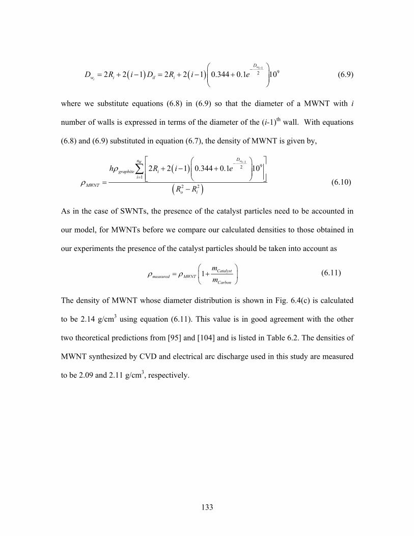
( ) ( )1
922 2 1 2 2 1 0.344 0.1 10wi
i
D
w i il iD R i D R i e−−⎛ ⎞
= + − = + − +⎜⎜⎝ ⎠
⎟⎟ (6.9)
where we substitute equations (6.8) in (6.9) so that the diameter of a MWNT with i
number of walls is expressed in terms of the diameter of the (i-1)th wall. With equations
(6.8) and (6.9) substituted in equation (6.7), the density of MWNT is given by,
( )
( )
192
1
2 2
2 2 1 0.344 0.1 10wiW
Dn
graphite ii
MWNTo i
h R i e
R R
ρ
ρ
−−
=
⎡ ⎤⎛ ⎞+ − +⎢ ⎥⎜ ⎟⎜ ⎟⎢ ⎥⎝ ⎠⎣ ⎦=
−
∑ (6.10)
As in the case of SWNTs, the presence of the catalyst particles need to be accounted in
our model, for MWNTs before we compare our calculated densities to those obtained in
our experiments the presence of the catalyst particles should be taken into account as
1 Catalystmeasured MWNT
Carbon
mm
ρ ρ⎛
= +⎜⎝ ⎠
⎞⎟ (6.11)
The density of MWNT whose diameter distribution is shown in Fig. 6.4(c) is calculated
to be 2.14 g/cm3 using equation (6.11). This value is in good agreement with the other
two theoretical predictions from [95] and [104] and is listed in Table 6.2. The densities of
MWNT synthesized by CVD and electrical arc discharge used in this study are measured
to be 2.09 and 2.11 g/cm3, respectively.
133

Figure 6.5(b): The density of SWNTs plotted as a function of the diameter of bundles.
Both computational (crosses, open triangles, and open circle) and experimental (solid
square, solid triangle, and solid diamond) densities are presented.
The density of acid-SWNT is measured to be 1.74 ± 0.04 g/cm3, which is 0.13
g/cm3 less than the density of p-SWNT (see Fig. 6.1 (a) and (b)). The decrease in the
density can be attributed to the structural transformation from p-SWNT to acid-SWNT.
The localized ultrasonication causing acidic oxidation disrupted the close-packed
triangular lattice formation of individual p-SWNTs. The carboxyl groups formed
subsequently at the ends and sides of the tubes made individual tubes hydrophilic thus
separating from each other in the water network. The scattered spatial disposition reduced
134

the density. In case of MWNTs we observed two bands, one close to the meniscus
corresponding to amorphous carbon and the second corresponding to MWNTs. However,
among all CNT structures, iso-SWNTs have the highest density (as can be seen in Table
6.1).
2 R i
2 R o
L
Dil
Figure 6.5(c). Illustration of MWNT based on the continuum hypothesis. The multi-shells
are treated as a continuum medium with thickness h and length L.
135
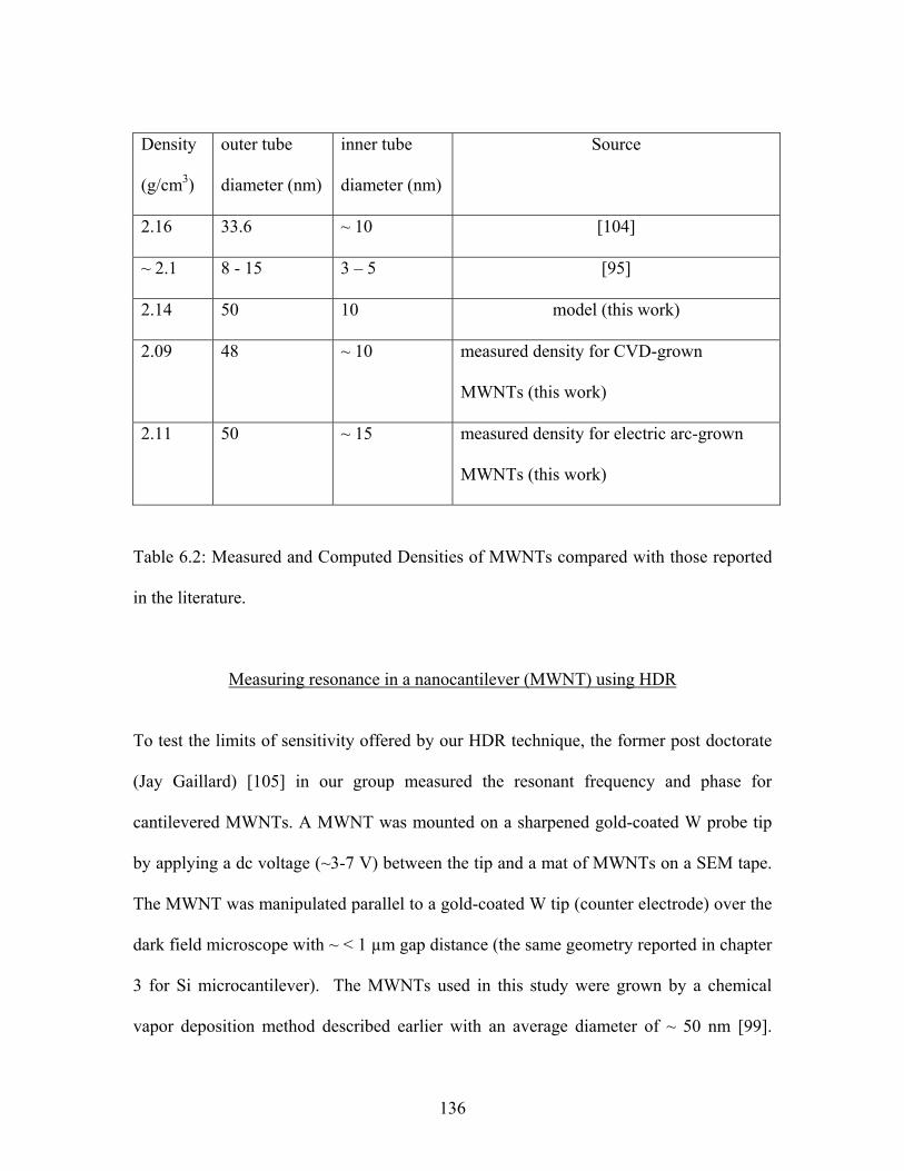
Density
(g/cm3)
outer tube diameter (nm)
inner tube diameter (nm)
Source
2.16 33.6 ~ 10 [104]
~ 2.1 8 - 15 3 – 5 [95]
2.14 50 10 model (this work)
2.09 48 ~ 10 measured density for CVD-grown
MWNTs (this work)
2.11 50 ~ 15 measured density for electric arc-grown
MWNTs (this work)
Table 6.2: Measured and Computed Densities of MWNTs compared with those reported
in the literature.
Measuring resonance in a nanocantilever (MWNT) using HDR
To test the limits of sensitivity offered by our HDR technique, the former post doctorate
(Jay Gaillard) [105] in our group measured the resonant frequency and phase for
cantilevered MWNTs. A MWNT was mounted on a sharpened gold-coated W probe tip
by applying a dc voltage (~3-7 V) between the tip and a mat of MWNTs on a SEM tape.
The MWNT was manipulated parallel to a gold-coated W tip (counter electrode) over the
dark field microscope with ~ < 1 µm gap distance (the same geometry reported in chapter
3 for Si microcantilever). The MWNTs used in this study were grown by a chemical
vapor deposition method described earlier with an average diameter of ~ 50 nm [99].
136

Figure 6.6 displays typical resonance and phase (shown in green open circles) spectra for
a MWNT. To verify the amplitude peak corresponding MWNT, the signal (shown in red
solid circles) in Fig. 6.6 in the absence of the MWNT for the same tungsten probe
geometry was compared with the amplitude signal (shown in blue solid circles) with
MWNT.
Figure 6.6: The amplitude (solid circles) and phase (open circles) spectra of a MWNT (7
µm long and 50 nm in diameter) near resonance measured under ambient conditions. The
inset shows an optical dark field image of the MWNT placed parallel to the W tip
(counter electrode) with 5 µm scale bar [2].
137

The second former post doctorate (Razvan Ciocan) [1] used a slightly different
geometry between the MWNT and W probe tip acting as a counter electrode for
measuring the resonance of MWNT. In this case, a gold-coated W probe tip is brought in
close proximity to and aligned with the MWNT over a dark field optical microscope as
shown in Fig. 6.7(a) An ac voltage (Vac) along with a dc voltage (Vdc) applied to counter
electrode induce charges on the MWNT. The electrostatic force, (FC) between the
charges residing on the MWNT and the counter electrode causes the MWNT to oscillate
(see Fig. 6.7(b)).
Figure 6.7 (a): Dark field microscope image of the geometrical setup for the MWNT and
the counter electrode assembly. The MWNT is facing the end of counter electrode in its
very close proximity (see text). (b) A schematic of mechanical oscillations induced in a
MWNT by the force (FC), when the MWNT and the counter electrode are separated by a
distance (s).
138

The typical resonance spectra for a CVD grown MWNT (10 µm long and 57 nm
in diameter) is shown in Fig. 6.7 (c). The resonant frequency at second mode for a
MWNT is around 2.42 MHz. No noticeable changes in the traces for the amplitude (dark
circles) and phase (dark triangles) can be discerned near resonance when the MWNT is
absent.
Figure 6.7 (c): The amplitude (light circles) and phase (light triangles) spectra near the
resonance of MWNT. The amplitude (dark circles) and phase (dark triangles) signals
obtained for the same geometry of W probe tip in the absence of MWNT.
139

For a MWNT clamped at one end, the resonant frequency (fi) of the ith mode of
vibration is given by [51],
(6.12) 2 2
2
(18
i ii
D DfL
βπ ρ
+=
2 )O E
where L is the tube length, Do and Di are the outer and inner tube diameters, respectively.
ρ is the density of the MWNT and the βi values are determined from the boundary
conditions to be β1 = 1.875, β2 = 4.694, and β3= 7.855 [51].
The experimentally measured resonant frequency of the MWNT (L = 10 µm, Di =
17 nm and D0 = 57 nm) at second mode is 2.42MHz as seen in Fig. 6.7 (c). The density
of a MWNT used for this calculation is determined using gradient sedimentation method
and listed in Table 6.2 as ρ = 2110 kg/m3. The bending modulus (E) of this MWNT is
computed using equation 6.12. Since three resonant frequencies are measured, three
values of E are calculated. A least squares fit to the data and gives E ~ 29.6 GPa [1].
Conclusions
The densities of carbon nanotube samples having various structures were
determined precisely with the equilibrium density gradient sedimentation technique using
sodium metatungstate as the gradient-generating agent. Bundled, isolated and acid-treated
SWNTs and MWNTs formed sharp well-defined bands at the respective densities. This
can be attributed to the differences in structural features of CNTs resulting in
distinguishable differences in densities. Transmission electron microscopy (TEM) and
140

micro-Raman spectroscopy provided significant evidence to confirm the structure of the
material in each band. The measured densities for bundled, isolated, and acid-treated
SWNTs and MWNTs are 1.87, 2.13, 1.74, and 2.1 g/cm3 respectively. These were found
to be in good agreement with the theoretical computations based on their structures. HDR
is an appropriate method to electrically actuate and detect resonances in nanoscale
cantilevers. Besides leading to nanoscale sensors, HDR is a powerful tool for determining
fundamental mechanical properties of 1D materials. As an example, the Young’s
modulus of CNTs has been discussed in this chapter. The key parameter, viz. the density
of CNTs, required in equation (6.12) was obtained by the gradient sedimentation method.
141

APPENDICES
142

Appendix A
Procedure for making sensor chip
Figure A-1: A schematic diagram showing all the steps involved in the procedure for
fabricating a sensor chip with two geometries for the electrodes. The left series show the
geometry wherein a rectangular gold strip acts as counter electrode whereas a tungsten tip
acting as counter electrode is depicted in the right series.
143

Two different geometries for the electrodes were developed and tested for
experiments described in this dissertation. The schematic of each step is shown in Fig. A-
1. In the first geometry, we start with a commercially available rectangular chip carrier
(0.5˝× 0.3˝) on which a quartz substrate (0.3˝ × 0.2˝) is glued using the 5 minute epoxy
(step 2). Next, a rectangular strip (0.15˝ × 0.0014˝) of gold (~ 80-100 nm thick) is
fabricated using standard masking wire technology and thin film evaporation (step 3).
This thin rectangular strip of gold acts as a counter electrode (Fig.A-1, left series). With
the help of a dark field microscope and a XYZ stage, a gold coated silicon
microcantilever (Micromasch, 35 µm wide, 2 µm thick and 350 µm long) is brought close
to the counter electrode and aligned parallel to the counter electrode with a gap distance
of ~ 8-10 μm. The HDR signals are monitored and the microcantilever position is
adjusted until a maximum signal is obtained (step 4). Then the cantilever is glued, and the
electrical contacts to the chip carrier are established (steps 5 and 6). Subsequently, we
had to develop an improved design for the counter-electrode since the field between the
gold stripe and the microcantilever often led to undesirable snapping of the
microcantilever into the gold stripe when driven into resonance at small gap distances.
This problem was overcome by using a conical-shaped tungsten tip (discussed in
Appendix B) as the counter electrode. Therefore, in our improved design we adopt an
identical procedure wherein the conical tip is first glued to the chip carrier, and the
microcantilever is manipulated and glued after strong HDR signals are obtained (Fig.A-1,
right series). This chip design was used for all experiments discussed in this dissertation.
144

Appendix B
Procedure for etching tungsten probe tips
Figure B-1: A Schematic of tungsten wire immersed in NaOH solution with a carbon rod
serving as an electrode. The tungsten tip etches from the bottom to the desired length in
this solution
The schematic for etching a tungsten tip is illustrated in Fig. B.1. A carbon rod
(dia. ~ 3 mm) serves as an one of the electrodes in a electrolyte (2 M NaOH solution in
145
de-ionized water) contained in a glass beaker. A 0.1 mm dia., tungsten wire is dipped
into this solution such that its tip is about 1 inch below the surface of the solution. The ac
voltage applied across the carbon rod and tungsten wire is controlled using a variac and it
results in a current flow between the wire and the rod. During the etching process,
bubbles rapidly form around the immersed wire making it difficult to see its tip. After
about 30 seconds of etching, the wire begins to reduce in length and diameter. When its
dipped length is etched from 1 inch to few (2-5) mm, the tip acquires a very sharp profile.
This method can easily etch the ends of the tips to ~100 nm in diameter and the sharpest
tip that we have etched in our lab so far is about 15 nm in diameter. The process takes
less than a minute, which allows the user to etch a large number of tips in a short period
of time. After etching the sharp tips, each tip is subjected to a three step cleaning process.
In first step, the tip is dipped in deionized water to dilute the NaOH followed by rinsing
with acetone which completely cleans off the residual NaOH. Finally it is again dipped in
purified water to clean off the acetone (since acetone leaves behind residue).
146

Appendix C
Operating principle of Mass flow controllers
Figure C-1: Alicat Scientific Mass flow controller used in order to control the flow rates
of different gases under study during our measurements. By clicking the MODE button
on the display we select the particular gas and on the next screen enter the required flow
rate [106].
We have used 16 Series Mass and Volumetric Precision Gas Flow Controller
(Fig. C-1) for all our measurements reported in chapter 5. All M and V Series Gas Flow
Meters are based on the accurate measurement of volumetric flow. The volumetric flow
rate is determined by creating a pressure drop across a unique internal restriction, known
147

as a Laminar Flow Element (LFE), and measuring the differential pressure across it. The
restriction is designed so that the gas molecules are forced to move in parallel paths along
the entire length of the passage; hence laminar (streamline) flow is established for the
entire range of operation of the device. In order to get an accurate volumetric flow rate,
the gas whose flow rate is being measured must be selected in the menu. This is
important because the device calculates the flow rate based on the viscosity of the gas at
the measured temperature. If the gas that is being measured is not what is selected in the
menu, an incorrect value for the viscosity of the gas will be used in the calculation of
flow, and the resulting output will be inaccurate in direct proportion to the difference in
the two gases viscosities.
Therefore, while studying the effect of deuterium (D2) on the response of
vibrating microcantilever in chapter 5, an equivalent flow rate of hydrogen (H2) was
calculated by taking into account the viscosities of H2 and D2.
2 2
2 2
H D
D H
ηη
= (C.1)
where Q is volumetric flow rate and η is the absolute viscosity of the particular gas.
Substituting QD2 = 100 sccm, ηD2 = 0.0001185 poise and ηH2 = 0.0000865 poise in
equation (C.1), we calculated the equivalent flow rate of H2. As D2 is not listed in the
select gas menu, we selected H2 in the menu of the mass flow controller and adjusted the
flow rate to 139 sccm in order to get 100 sccm of deuterium.
148

Appendix D
Equipment List
1. Stanford Research Systems SR 830 Lock-in Amplifier.
2. Stanford Research Systems DS345, 30 MHz synthesized Functional generator.
3. Amptek (A-250) charge sensitive pre-amplifier.
4. Epiphot 200 dark field/bright field microscope with a 50x, 8.4 mm long working
distance objective lens.
5. TRIAX 550 single-grating Raman spectrometer (groove density 1200
grooves/mm) equipped with a liquid nitrogen-cooled charge-coupled device
(CCD).
6. Beckman centrifuge with SW56 rotor.
7. Hitachi 7600 Transmission electron microscope.
149

REFERENCES
[1] R. Ciocan et al., Nano Lett. 5, 2389 (2005). [2] J. Gaillard et al., Rev. Sci. Instrum. 77, 073907 (2006). [3] G. Keskar et al., Sens. Actuators A (2008). [4] G. Keskar et al., IEEE Sensors J. (2008). [5] G. Keskar et al., Sens. and Transducers 91, 1 (2008). [6] H. L. Tuller, and R. Micak, Current Opinion in Solid State & Materials Science 3,
501 (1998). [7] V. L. Nickolay, J. S. Michael, and G. D. Panos, Review of Scientific Instruments
75, 2229 (2004). [8] C. Ziegler, Anal Bioanal Chem 379, 946 (2004). [9] D. Then, A. Vidic, and C. Ziegler, Sensors and Actuators B-Chemical 117, 1
(2006). [10] P.G. Datskos, T.Thundat, and V. L. Nickolay, Encyclopedia of Nanoscience and
Nanotechnology 5, 551 (2004). [11] P. L. and, and X. Li, J. Micromech. Microeng. 16, 2539 (2006). [12] F. M. Battiston et al., Sensors and Actuators B-Chemical 77, 122 (2001). [13] T. Thundat, a. P. I. Oden, and R. J. Warmack, Microcantilever Sensors
(Microscale Thermophysical Engineering, 1997), Vol. 1, p. 185. [14] P. I. Oden et al., Appl. Phys. Lett. 68, 3814 (1996). [15] J. Fritz et al., Science 288 (2000). [16] M. K. Baller et al., Ultramicroscopy 82, 1 (2000). [17] R. Raiteri, and H. J. Butt, Journal of Physical Chemistry 99, 15728 (1995). [18] S. J. Oshea et al., Journal of Vacuum Science & Technology B 14, 1383 (1996).
150
[19] D. R. Baselt, G. U. Lee, and R. J. Colton, Journal of Vacuum Science & Technology B 14, 789 (1996).
[20] Z. Y. Hu, T. Thundat, and R. J. Warmack, Journal of Applied Physics 90, 427
(2001). [21] T. Thundat et al., Applied Physics Letters 64, 2894 (1994). [22] P. G. Datskos, and I. Sauers, Sensors and Actuators B-Chemical 61, 75 (1999). [23] H. P. Lang et al., Analytica Chimica Acta 393, 59 (1999). [24] D. Lange et al., in Smart Structures and Materials1998), pp. 233. [25] R. Berger et al., Microelectronic Engineering 35, 373 (1997). [26] T. Thundat et al., Applied Physics Letters 66, 1695 (1995). [27] T. Thundat et al., Applied Physics Letters 66, 1563 (1995). [28] C. Rossel et al., Journal of Applied Physics 79, 8166 (1996). [29] R. P. Cowburn, A. M. Moulin, and M. E. Welland, Applied Physics Letters 71,
2202 (1997). [30] S. Porthun, L. Abelmann, and C. Lodder, Journal of Magnetism and Magnetic
Materials 182, 238 (1998). [31] C. F. Q. G. Binning, C. Gerber, Phys. Rev. Lett 56 (1986). [32] R. Berger et al., Applied Physics Letters 69, 40 (1996). [33] J. R. Barnes et al., Nature 372, 79 (1994). [34] J. K. Gimzewski et al., Chemical Physics Letters 217, 589 (1994). [35] Rüdiger Berger et al., Science 276 (1997). [36] R. Berger et al., Chemical Physics Letters 294, 363 (1998). [37] H. Wenhai, S. M. Lindsay, and J. Tianwei, Applied Physics Letters 69, 4111
(1996). [38] A. Schemmel, and H. E. Gaub, Review of Scientific Instruments 70, 1313 (1999).
151

[39] F. Ernst-Ludwig et al., Review of Scientific Instruments 65, 639 (1994). [40] M. A. Lantz, S. J. O. Shea, and M. E. Welland, Applied Physics Letters 65, 409
(1994). [41] R. Irene, and P. Roger, Journal of Applied Physics 87, 526 (2000). [42] S. J. O'Shea et al., Nanotechnology 16, 602 (2005). [43] J. Teva et al., Ultramicroscopy 106, 808 (2006). [44] I. Voiculescu et al., Ieee Sensors Journal 5, 641 (2005). [45] D. Rugar, H. J. Mamin, and P. Guethner, Applied Physics Letters 55, 2588
(1989). [46] G. Meyer, and N. M. Amer, Applied Physics Letters 53, 1045 (1988). [47] P. Poncharal et al., Science 283, 1513 (1999). [48] M.-F. Yu et al., Physical Review B 66, 073406 (2002). [49] S. T. Purcell et al., Physical Review Letters 89, 276103 (2002). [50] J. Gaillard, M. Skove, and A. M. Rao, Applied Physics Letters 86, 233109 (2005). [51] Z. L. Wang, P. Poncharal, and W. A. de Heer, Pure and Applied Chemistry 72,
209 (2000). [52] P. I. Oden et al., Applied Physics Letters 69, 3277 (1996). [53] M. Tortonese, R. C. Barrett, and C. F. Quate, Applied Physics Letters 62, 834
(1993). [54] V. Ferrari et al., Ieee Transactions on Ultrasonics Ferroelectrics and Frequency
Control 43, 601 (1996). [55] D. L. DeVoe, and A. P. Pisano, Journal of Microelectromechanical Systems 6,
266 (1997). [56] C. L. Britton et al., Ultramicroscopy 82, 17 (2000). [57] J. Verd et al., Journal of Microelectromechanical Systems 14, 508 (2005).
152
[58] G. Abadal et al., Nanotechnology 12, 100 (2001). [59] K. L. Ekinci, and M. L. Roukes, Review of Scientific Instruments 76, 061101
(2005). [60] M. D. Ventra, S. Evoy, and J. R. Helfin, Introduction to Nanoscale Science and
Technology (Springer, New York, 2004), pp. 405. [61] J. F. Nye, Physical properties of crystal (Oxford press, 1957), p. 144. [62] M. P. Blencowe, and M. N. Wybourne, Applied Physics Letters 77, 3845 (2000). [63] A. Bertz et al., Sensors and Actuators a-Physical 93, 163 (2001). [64] J.D. Taylor et al., in Frontiers in Nanoscience and Nanotechnology, edited by A.
N.,Y. Fu (Oxford University Press 2008). [65] http://www.angelfire.com/electronic2/spm/etching.html [66] S. Bianco et al., J. Vac. Sci. Technol. B 24, 1803 (2006). [67] S. Weigert, a. M. Dreier, and M. Hegner, Appl. Phys. Lett. 69, 2834 (1996). [68] F. Shen et al., Sens. Actuators A 95, 17 (2001). [69] R. Sandberg et al., J. Micromech. Microeng. 15, 1454 (2005). [70] J. Mertens et al., Ultramicroscopy 97, 119 (2003). [71] F. R. Blom et al., J. Vac. Sci. Technol. B 10, 19 (1992). [72] L. D. L. and, and E. M. Lifshitz, Course of Theoritical Physics (Butterworth
Washington, DC/Heinemann, London, 1987), Vol. 6. [73] R. G. Christian, Vacuum 16, 175 (1966). [74] A. B. Pippard, The Physics of Vibration (Cambridge University Press, Cambridge,
1978), Vol. 1, p. 252. [75] H. Hosaka, K. Itao, and S. Kuroda, Sensors and Actuators a-Physical 49, 87
(1995). [76] D. Sarid, Scanning Force Microscopy (Oxford, New York, 1994), p. 169.
153

[77] A. Isacsson, J. M. Kinaret, and R. Kaunisto, Nanotech. 18, 195203 (2007). [78] S. Zaitsev et al., IEEE proceedings (2006). [79] H. W. Ch. Postma et al., App. Phys. Lett 86, 223105 (2005). [80] I. Kozinsky et al., App. Phys. Lett 88, 253101 (2006). [81] R. Almog et al., Phys. Rev. Lett 98, 078103 (2007). [82] S. K. De., and a. N. R. Aluru, J. Microelectromech. Sys. 15, 355 (2006). [83] A. H. Nayfeh, and D. T. Mook, Nonlinear oscillations (Wiley - Interscience,
1995), pp. 163. [84] M. V. Requa, and K. L. Turner, App. Phys. Lett 88, 263508 (2006). [85] J. J. Yao, and N. C. MacDonald, J. Micromech. Microeng. 6, 257 (1996). [86] J. S. Aldridge, and A. N. Cleland, Phys. Rev. Lett. 94, 156403 (2005). [87] L. A. Pinnaduwage et al., Appl. Phys. Lett. 83, 1471 (2003). [88] Certified Air Safety (http://www.certifiedairsafety.com). [89] B. Plewinsky, and R. Kamps, Makromolekulare Chemie-Macromolecular
Chemistry and Physics 185, 1429 (1984). [90] M. Terrones, Annual Review of Materials Research 33, 419 (2003). [91] J. Chen et al., Science 282, 95 (1998). [92] S. Ciraci et al., Journal of Physics-Condensed Matter 16, R901 (2004). [93] D. Tasis et al., Chemical Reviews 106, 1105 (2006). [94] G. H. Gao, T. Cagin, and W. A. Goddard, Nanotechnology 9, 184 (1998). [95] Q. Huang et al., Journal of Materials Chemistry 15, 1995 (2005). [96] Manual of Weighing Applications, Part 1; Sartorius AG: Gottingen,,Germany,
2004.See http://www.sartorius.com/fileadmin/sartorius_pdf/ Prospekt/englisch/DensityDeterminationManual.pdf.
154

155
[97] Q. Lu et al., Journal of Physical Chemistry B 110, 24371 (2006). [98] K. A. Williams et al., Nature 420, 761 (2002). [99] R. Andrews et al., Chemical Physics Letters 303, 467 (1999). [100] R. B. Mathur et al., in National Conference on Carbon, Indo-Carbon2001), p.
226. [101] A. M. Rao et al., Science 275, 187 (1997). [102] C. H. Kiang et al., Physical Review Letters 81, 1869 (1998
http://www.wag.caltech.edu/foresight/foresight_2.html.). [103] S. Govindjee, and J. L. Sackman, Solid State Communications 110, 227 (1999). [104] D. Qian et al., Applied Physics Letters 76, 2868 (2000). [105] J. B. Gaillard, in Department of Physics and Astronomy (Clemson University,
Clemson, 2006). [106] Alicat Scientific (http://www.alicatscientific.com).