inference of surface concentrations of nitrogen dioxide ... · inference of surface concentrations...

Atmósfera 27(2), 193-214 (2014)

Inference of surface concentrations of nitrogen dioxide (NO2) in Colombia from tropospheric columns of the ozone measurement instrument (OMI)

JOHN FREDDY GRAJALES and ASTRID BAQUERO-BERNALGrupo de Simulación del Sistema Climático Terrestre, Departamento de Física, Universidad Nacional de Colombia,

Cra. 30 45-03, Bogotá, ColombiaCorresponding author: A. Baquero-Bernal; e-mail: [email protected]

Received March 23, 2013; accepted March 8, 2014

RESUMEN

Por primera vez se presentan mapas de concentración superficial de dióxido de nitrógeno (NO2) para el te-rritorio colombiano. Se infirieron concentraciones superficiales de NO2 para 2007 a partir de dos fuentes de datos de densidad de columna troposférica: 1) una simulación que utiliza el modelo global tridimensional GEOS-Chem y 2) mediciones realizadas por el instrumento de monitoreo del ozono (OMI, por sus siglas en inglés) instalado a bordo del satélite Aura de la NASA. Los resultados muestran valores mensuales promedio de 0.1 a 6 ppbv. Se compararon las concentraciones superficiales de NO2 inferidas con mediciones in situ corregidas y se encontraron coeficientes de correlación de hasta 0.91. Una fuente importante de NO2 es la quema de biomasa, la cual puede ser diagnosticada a partir de los datos de potencia radiativa de los fuegos provenientes del reanálisis para el monitoreo de la composición atmosférica y el clima (MACC, por sus siglas en ingés). Se encontró una fuerte relación entre altas concentraciones de NO2 inferidas y quema de biomasa para un área extensa que comprende los departamentos de Caquetá, Meta, Guaviare, Vichada y Putumayo.

ABSTRACT

For the first time, maps of surface concentration of nitrogen dioxide (NO2) are presented for the Colombian territory. NO2 surface concentrations for the year 2007 are inferred based on two sources of tropospheric NO2 column data: (1) a simulation using a three-dimensional global model (GEOS-Chem) and (2) measurements made by the ozone monitoring instrument (OMI) onboard the NASA Aura satellite. Results show monthly averages between 0.1 and 6 ppbv. We compare these inferred values to corrected ground measurements of NO2. We find correlation coefficients of up to 0.91 between the inferred data and the corrected observational data. A significant source of NO2 is biomass burning, which can be diagnosed by data of fire radiative power (FRP) from the Monitoring of Atmospheric Composition and Climate (MACC) reanalysis. We find a close relationship between high values of inferred NO2 surface concentrations and biomass burning for a large area which encompasses the departments of Caquetá, Meta, Guaviare, Vichada, and Putumayo.

Keywords: Inference of nitrogen dioxide surface concentration, density of tropospheric columns, OMI, GEOS-Chem, fire radiative power, chemiluminescence interference, overestimation, Colombia.

1. IntroductionNO2 is both an important contributor to ozone (O3) decomposition in the stratosphere and a major pre-cursor in the chain of chemical reactions that produc-es O3 in the troposphere. Both O3 and NO2 are toxic to biota. Long-term exposure to NO2 is significantly associated with decreased lung function and is a risk

factor for respiratory diseases (Ackermann-Liebrich, 1997; Schindler et al., 1998; Gauderman, 2000, 2002; Panella et al., 2000; Smith et al., 2000). The measurement of pollutants not only allows the track-ing of anthropogenic activity, but also improves our understanding of the relationships between pollution and natural phenomena. In this study, we focus on

194 J. F. Grajales and A. Baquero-Bernal

NO2. Nitrogen oxide (NO) and NO2 species are pro-duced from lightning, biomass burning, fossil fuel combustion, and soils (Sauvage et al., 2007). The high temperatures of combustion break down mo-lecular oxygen (O2) from the air, which subsequently enters an important chemical reaction that produces NO and NO2 (Jacob, 1999). Their production in combustion makes NOx a marker of industrial ac-tivity (including fossil fuel-based power generation, transportation, and concrete manufacture) as well as other human activities, such as agricultural biomass burning. Therefore, NO2 serves as an indicator of air quality and anthropogenic activity. Researchers have made significant efforts to analyze pollutant emission and overall air quality in Colombia, but none were focused specifically on NO2 (Lacouture, 1979; Be-doya, 1981; Ruiz, 2002; Benavides, 2003; Barreto, 2004; Jiménez, 2004; Oviedo, 2009).

Our primary interest in this study is the inference of surface NO2 concentrations in Colombia. To infer these concentrations, we use the GEOS-Chem tro-pospheric chemistry model along with tropospheric column data from the ozone-measuring instrument (OMI) onboard the NASA Aura satellite. The first step of the inference process was the acquisition of NO2 tropospheric column data from the OMI. We use the OMNO2e product (Kempler, 2010). There are other OMI products that report NO2 density of tropospheric columns, such as the different products of the Royal Netherlands Meteorological Institute (KNMI) (Boersma et al., 2007, 2011). However, the analysis of these products and their intercomparison are beyond the scope of this study.

Aerial measurements reveal that the concentration of NO2 in the tropospheric column is determined pri-marily by NO2 in the mixed layer, as well as by that in the boundary layer (Martin et al., 2004, 2006; Boersma et al., 2008; Bucsela et al., 2008). However, the pro-portion of NO2 in these two layers varies in space and time. Lamsal et al. (2008) proposed a method that uses the local NO2 profiles obtained from the GEOS-Chem model to capture this variation in space and time. The GEOS-Chem model is a global three-dimensional model of tropospheric chemistry driven by assimilated meteorological observations from the Goddard Earth Observing System (GEOS) of the NASA Data Assim-ilation Office (Bey et al., 2001; Gass, 2012; Rienecker et al., 2008). This model provides a comprehensive description of atmospheric composition and allows us

to obtain tropospheric column densities and profiles up to 0.01 hPa. These profiles are used together with the tropospheric column data from OMI (see details in section 4.5) to infer quasi-observed concentrations of NO2 at the surface.

Celarier et al. (2008) validated the tropospheric, stratospheric and total NO2 columns from the OMI with respect to surface measurements from multiple sources. This validation is difficult for many reasons, perhaps the most important of which is that each OMI column corresponds to the average over a large area (at least 340 km2), whereas surface measurements are site-specific. In addition, surface measurement instruments are often placed at points of maximum emission and, therefore, do not measure background concentrations. Another difficulty is that the length of each time data series for validation is short, and the number of series is small, which makes statistical analysis difficult. Despite these and other difficulties, OMI measurements and surface measurements yield correlations in the data that are generally above 0.6. Another way to validate the tropospheric columns is through air campaigns or in situ experiments, which provide vertical profile data. Boersma et al. (2008) reported a high similarity between OMI data and in situ profile data.

For the first time, maps of surface concentration of NO2 are presented for the Colombian territory for a whole year, 2007. Additionally, in order to assess the contribution of the biomass burning to the NO2 concentrations in the country, the inferred surface NO2 concentrations are compared with fire radia-tive power data, which is used to monitor biomass burning. A brief summary of all the datasets used is given in section 2. Section 3 describes the methods used to infer the surface concentrations of NO2 and to calculate the correction factors to NO2 concentra-tions measured at surface stations. The results and conclusions are presented in sections 4 and 5.

2. Data2.1 NO2 tropospheric column from OMIWe used data from the OMNO2e product, which is a daily, global, gridded data product, where each file is produced from one day’s worth of NO2 measurements made by the ozone monitoring instrument onboard the EOS-Aura spacecraft (OMI Team, 2009). The data are filled into a grid with horizontal resolution of 0.25 × 0.25º in latitude and longitude. The data fields included in the product are two: (a) total column NO2

195Surface concentrations of NO2 in Colombia

in units of molecules/cm2, cloud-screened at 30%; and (b) tropospheric column NO2, cloud-screened at 30%. For each grid cell a field-of-view (FOV) weight-ed estimate was calculated for each field (Bucsela et al., 2006; Kempler, 2010). The Aura satellite passes over Colombian territory at 17:00 and 18:00 UTC or 12:00 and 13:00 LT.

The reported NO2 column corresponds to the visible range (between 405 and 465 nm), i.e., in the presence of clouds, the amount of NO2 reported corresponds to the amount found above these. The maximum detection limit for a cloudy area is 30%, meaning that when cloud cover is below this value, there should be no bias in the data calculated using the standard algorithm (Torres et al., 2002). For grid cells with cloud covers above 30%, both total and tropospheric NO2 columns are set to missing values.

2.2 GEOS-Chem simulationTo infer the NO2 concentrations at the surface, infor-mation about the NO2 tropospheric profile is required. To obtain this profile, we used the GEOS-Chem 3D global tropospheric chemistry model. The GEOS-Chem simulation performed is of the type “NOx-Ox-hy-drocarbons” and has a spatial resolution of 2.5 × 2º. GEOS-Chem simulates tropospheric ozone-nitrogen oxides-hydrocarbon chemistry. We used version v8-02-01, in which there are 43 advected tracers. The simulation with GEOS-Chem was performed for 47 vertical levels that ranged from the surface to 0.01 hPa, and covers the years 2006 and 2007. The year 2006 served as a model spin-up. The simulation includes the reaction mechanisms SMVGEAR II and FAST-J for photolysis (Evans et al., 2003).

Although there are emissions inventories for some cities, there is no national emission inventory avail-able for Colombia. For this reason, we used the de-fault inventories suggested by the GEOS-Chem team according to the region of the world (see Table 2 in http://acmg.seas.harvard.edu/geos/word_pdf_docs/emissions_v8_02_03.pdf). In particular for Central and South America, the NOx, SOx and CO emissions are from EDGAR 3.2 FT (Olivier and Berdowski, 2001); the VOC and NH3 emissions are from GEIA (Wang et al., 1998); and BC/OC emissions are from Bond et al. (2007). Emissions from open fires for individual years were taken from the monthly GFED2 inventory (van der Werf et al., 2009). The emissions are available from 1997 to 2008 (see item

4.2.16 in http://acmg.seas.harvard.edu/geos/doc/man/chapter_4.html), so the fires occurring in 2007 are included in the model on a monthly basis.

2.3 Surface data from air quality stationsTo validate the inferred surface concentrations, we used NO2 data from stations of the air quality monitoring networks installed in Bogotá and Bucar-amanga (Fig. 1) by the Secretaría Distrital de Ambi-ente (District Department of Environment) and the Corporación Autónoma Regional para la Defensa de la Meseta de Bucaramanga (Regional Autonomous Corporation for the Defense of the Bucaramanga Plateau), respectively. For Bogotá, we used data from seven stations: IDRD, MAVDT, Fontibón, Las Ferias, Suba, Puente Aranda, and Carvajal. For Bucaraman-ga, we used data from the Centro station. These data represent measurements made using commercial chemiluminescence equipment.

All of the NO2 data used in this study represent values measured between 17:00 and 19:00 UTC. The period of greatest coverage of the Colombian territory by the Aura satellite is between 17:00 and 19:00 UTC (12:00 and 14:00 LT). For this reason, the NO2 data obtained from each source (in situ, OMI and GEOS-Chem) were averaged for these two hours. Subsequently, monthly averages for each NO2 data-set were calculated using these values only at those days when OMI data are available. Table I shows an overview of the data used in this work.

3. Methodology3.1 Inference of surface concentrations of NO2

Lamsal et al. (2008) proposed a method that uses the local NO2 profile obtained from the GEOS-Chem model to capture the variation in space and time of the NO2 concentration. Based on the GEOS-Chem profiles, the OMI concentrations at the surface can be estimated as follows:

S0 =SG

* Ω0ΩG (1)

In this equation, S represents the superficial level concentration, and Ω represents the NO2 tropospheric column. The subindex O indicates OMI, and the sub-index G indicates GEOS-Chem. The OMI-derived surface concentration So represents the mixing ratio in the lowest layer of the model, which is approxi-mately 70 m (Le Sager et al., 2008).


The spatial variation of the OMI observations (which have an original resolution of 0.25 × 0.25º) within the resolution of the GEOS-Chem simulation

(2.5 × 2º) should reflect variation in NO2 concentra-tions within the boundary layer. Lamsal et al. (2008) developed a scheme to combine both sources of

Table I. Overview of the NO2 data used.

Type Measurement Method Available time

OMI Tropospheric column of NO2 Satellite 17-19 UTC or 12-14 LT

GEOS-Chem NO2 Tropospheric columnand NO2 surface concentration(level 1 of model)

Model simulation Hourly

Ground stations at Bogotá and Bucaramanga

Surface concentrations of NO2.

Chemiluminescence Hourly

Number Department114N

12N

10N

8N

6N

4N

2N

EQ

2S

4S

80 78 76 74 72 70 68

Amazonas2 Antioquia3 Arauca4 Atlántico5 Bolivar6 Boyacá7 Caldas8 Caquetá9 Casanare

10 Cauca11 Cesar12 Chocó13 Córdoba14 Cundinamarca15 Guainía16 Guaviare17 Huila18 La Guajira19 Magdalena20 Meta21 Nariño22 Norte de Santander23 Putumayo24 Quindio25 Risaralda

2627 Santander28 Sucre29 Tolima30 Valle del Cauca31 Vaupés32 Vichada

San Andrés, Providencia and Santa Catalina

Lat.

(º)

Long. W (º)

Fig. 1. Political map and topography of Colombia. For this study, in situ measurements were available only from those stations indicated by black circles (Bogotá and Bucaramanga). Beyond the Colombian Massif (in the south-western departments of Nariño and Cauca) the Andes are divided into three branches known as cordilleras (mountain ranges): the Cordillera Occidental (West Andes), the Cordillera Central (Central Andes), and the Cordillera Oriental (East Andes).


information (vertical profile and horizontal variation) to infer concentrations of NO2 at the OMI resolution, as follows:

S'0 =vSG

* Ω0vΩG – vΩG + ΩGF F (2)

In Eq. (2), Sʹo is the surface level NO2 concentra-tion, ν is a factor that describes the influence of the lower levels of the troposphere in the mixture of NO2, and ΩG

F corresponds to the free tropospheric column, which is taken as a horizontal constant on the GEOS-Chem grid and reflects the longest NO2 half-life in the free troposphere. The calculation of ΩG

F determines the planetary boundary layer and calculates the ex-isting column at and above this layer. ν is given by:

v =Ω0

Ω0 (3)

In this equation, Ω0 corresponds to the NO2 tro-pospheric columns from the OMI (0.25 × 0.25º), and Ω0 corresponds to the OMI tropospheric columns averaged at the GEOS-Chem grid resolution (2.5 × 2.0º). Eq. (2) becomes Eq. (1) when ν is equivalent to unity.

3.2 Interference in the measurement of NO2

Once the surface concentrations of NO2 are inferred, it is necessary to validate these concentrations. The NO2 measuring instrument most commonly used by air quality monitoring networks globally is the che-miluminescence analyzer, which contains a catalytic molybdenum converter (Ellis, 1975). This instrument is subject to significant interference from other oxi-dized substances, such as peroxyacytyl nitrate (PAN), nitric acid (HNO3), and organic nitrates (Grosjean and Harrison, 1985; Dunlea et al., 2007; Steinbacher et al., 2007). To correct this interference at the surface, correction factors (CF) were calculated using the GEOS-Chem model. Fig. 1 shows the location of the stations, from which in situ measurements were available for this study.

Commercial chemiluminescence detectors are powered by the intensity of light produced by the chemical reaction between ozone (provided by the measuring instrument) and NO, as follows:

NO+O3 NO2*+O2 (R1)

NO2* NO2 + h (R2)

In this reaction, NO2* corresponds to an excited NO2 molecule, which will subsequently lose a mea-surable amount of energy. This process involves the chemical reduction of NO and the use of a molyb-denum catalytic converter heated to 300-400 ºC to catalyze the chemiluminescence reaction described above. The instrument has two modes of measure-ment: NO and NOx. The concentration of NO2 is determined by subtracting the two reading modes (NOx-NO). The disadvantage of this approach is that not only NO2 is chemically reduced; other species, such as HNO3, PAN, and alkyl nitrate (AN), can also contribute. We used the CF developed by Lamsal et al. (2008) to correct our estimate of the concentration of surface NO2:

CF=NO2

NO2+∑AN + 0.95 PAN + 0.35HNO3 (4)

4. Results4.1 NO2 columns from the GEOS-Chem modelFigure 2 shows the monthly mean density of tropo-spheric NO2 columns obtained from the GEOS-Chem model simulation for Colombia. To calculate the monthly means, the model data was sampled only at those times when OMI data is available. The density of the tropospheric columns is relatively low, with values not exceeding 1.0 × 1015 molecules/cm2. The column density varies by region. Lower values (≈ 0.2 × 1015 molecules/cm2) are observed in southern and southeastern Colombia in departments that con-tain notable rainforest areas, including Amazonas, Caquetá, Putumayo, Vaupés, Guaviare, and Guainía. Slightly higher tropospheric column values (> 0.4 × 1015 molecules/cm2) are observed in northern Colom-bia in such departments as Córdoba, Sucre, Bolívar, Atlántico, Magdalena, Cesar, and La Guajira (as well as in Venezuela). Figure 2 also shows that in some cases, consecutive months have similar tropospheric NO2 column averages.

4.2 Surface NO2 concentrations from the GEOS-Chem modelThe surface level NO2 concentrations from the GEOS-Chem model are presented in Figure 3. Relatively low NO2 surface concentration values were obtained over most of Colombia. Lower values were observed in the southern, southeastern and Pacific regions, where anthropogenic activity is low or nonexistent,


and slightly higher values (up to 0.5 ppbv) were observed to the north along the Caribbean coast into Venezuela, where population density, agriculture, and industrial and mining activities are the greatest. This pattern is similar to that observed in the tropospheric column data from GEOS-Chem, which reflects the expected distribution of pollutants, as in forested areas or areas with little population, the surface

concentration of NO2 should be low compared to that observed in more populated areas or in areas of agricultural or industrial activities. This suggests a strong influence of the lower layers on the general properties of the tropospheric NO2 column, probably because chemically formed NO2 is generated mainly through land use and the burning of both fuels and biomass.

February

2

1.5

1

0.5

0.10.2

2

1.5

1

0.5

0.10.2

April June

DecemberOctoberAugust

Lat.

(º)

4S

2S

2N

4N

6N

8N

10N

12N

EQ

Lat.

(º)

4S

2S

2N

4N

6N

8N

10N

12N

EQ

79 78 77 76 75 74 73 72 71 70 69 68 67 66 65 79 78 77 76 75 74 73 72 71 70 69 68 67 66 65 79 78 77 76 75 74 73 72 71 70 69 68 67 66 65Long. W (º) Long. W (º) Long. W (º)

Fig. 2. Monthly average densities (in molecules/cm2 [× 1015]) of tropospheric NO2 columns from the GEOS-Chem model. Only the maps for even months are shown. For the calculation of the monthly averages, each grid cell of the density data (available in a resolution of 2.5 × 2.0º) was divided into 80 grid boxes of equal size (0.25 × 0.25º). Additionally, the GEOS-Chem density data was sampled only at those times when OMI data is available. Blank (white) grid boxes represent missing OMI data.


4.3 NO2 columns from OMIThe density values of the tropospheric NO2 columns from the OMI are shown in Figure 4. As was true for the GEOS-Chem data, we can see that in general, for most months, lower values are found in the south-ern and southeastern areas comprising departments with rainforest areas, including Amazonas, Vaupés, Guainía, Putumayo, Caquetá, and Guaviare. Another area with low concentration values is the Pacific region to the west, which includes departments of Chocó, Valle del Cauca, Cauca, and Nariño. Higher values are found mainly to the north, in departments

such as Córdoba, Sucre, Bolívar, Magdalena, Atlán-tico, and Cesar, as well as in Venezuela. The month with the lowest density values for the whole country is June. On the other hand, high-density values were reported by the OMI in February. In this month, a continuous strip of densities of 2 × 1015 molecules/cm2 or greater is observed between western Ven-ezuela and the departments of Vichada, Arauca, Casanare, Meta, and Caquetá, which are not densely populated. However, oil extraction is the main eco-nomic activity in the last four departments and in western Venezuela. The strip occurs in January (and

February

Lat.

(º)

4S

2S

2N

4N

6N

8N

10N

12N

EQ

Lat.

(º)

4S

2S

2N

4N

6N

8N

10N

12N

EQ

April June


34

2

1

0.5

0.25

0.2

0.15

0.1

0.05

34

2

1

0.5

0.25

0.2

0.15

0.1

0.05


Fig. 3. Monthly averages of NO2 surface concentration (in ppbv) from the GEOS-Chem model. Same remarks as in Figure 2.


also in December), covering western Venezuela and the departments of Vichada, Arauca, and Casanare, then reaches a maximum in February and declines approximately in April. At its peak, this continuous strip of high concentrations extends to the southwest and eastward to Caquetá, Putumayo, and Guaviare. These relatively high concentrations of NO2 may be associated with such factors as biomass burning, improper agricultural soil management, burning associated with the oil industry or the transport of NO2

from other regions.

4.4 Comparison of GEOS-Chem columns and OMI columnsFigure 5 shows the result of subtracting monthly OMI column densities from GEOS-Chem column densities (Figs. 4 and 2, respectively). To perform this subtraction, each grid cell of the GEOS-Chem data, available in a resolution of 2º × 2.0º, was di-vided into 80 grid cells of equal size (0.25 × 0.25º). Additionally, the GEOS-Chem data was sampled only at those times when OMI data is available. In general, tropospheric column densities from OMI are

February April June


Lat.

(º)

4S

2S

2N

4N

6N

8N

10N

12N

EQ

Lat.

(º)

4S

2S

2N

4N

6N

8N

10N

12N

EQ

6

5

4

3

21.5

1

0.5

0.1

6

5

4

3

21.5

1

0.5

0.1


Fig. 4. Monthly average densities of tropospheric NO2 columns (in molecules/cm2 [× 1015]) from the OMI for 2007. Grid resolution is 0.25 × 0.25º. Blank (white) grid boxes represent missing data. Only the maps for even months are shown.


systematically higher than those from GEOS-Chem. However, there are spots where column densities from OMI are lower than those from GEOS-Chem. These spots are mountain areas located on the Cor-dillera Oriental, Cordillera Occidental, Ecuadorian Andes, and Venezuelan Andes. There are also some spots located to the north, in the departments Guajira, Cesar, and Magdalena.

In Colombian remote regions, industrial activity is very little and volcanic activity is scarce. When there is not biomass burning in these regions, NO2

columns are determined by both lightning produc-tion and transport of pollutants from other regions. Therefore, density of tropospheric NO2 columns over these regions should have values close to zero. That should occur in departments of Amazonas and Vaupés and in parts of the departments of Guanía, Vichada, Caquetá, and Guaviare. In these regions, OMI (GEOS-Chem) columns have density values between 0.4 and 1.5 (0 and 0.8) × 1015 molecules/cm2 (see Figs. 2 and 5). Thus, there is overestimation of OMI columns in remote regions.

February April June


Lat.

(º)

4S

2S

2N

4N

6N

8N

10N

12N

EQ

Lat.

(º)

4S

2S

2N

4N

6N

8N

10N

12N

EQ

5

43

2

1

0.5

0

–0.5

5

43

2

1

0.5

0

–0.5


Fig. 5. Mean differences between OMI and GEOS-Chem monthly tropospheric NO2 columns (in molecules/cm2 [× 1015]). Only the maps for even months are shown.


Validation of satellite observations of tropospheric NO2 columns has been carried out in non-remote regions by both using differential optical absorption spectroscopy (Celarier et al., 2008) and by perform-ing aircraft measurements over the US and Mexico (Boersma et al., 2008). These authors reported that correlations between in situ NO2 measurements and satellite observations in some remote areas are not greater than 0.6.

To quantify the overestimation of NO2 column densities in remote regions by OMI, a bias correc-tion value is calculated as the average of all the

monthly differences between OMI and GEOS-Chem column densities for year 2007 and for all the grid points comprised in two rectangular areas: 1.50º N to 0.75º S, 71.50 to 70.00º W, and 0.75 to 2.25º S, 73 to 69.5º W. These two areas comprise the major part of the departments of Vaupés and Amazonas. A bias correction value of 0.4 × 1015 molecules/cm2 was found. Therefore, we propose that on points where the density of OMI NO2 columns is expected to be very low, this value should be subtracted.

From Eqs. (1) and (2) it can be inferred that if the tropospheric column density in a given area is

February April June


Lat.

(º)

4S

2S

2N

4N

6N

8N

10N

12N

EQ

Lat.

(º)

4S

2S

2N

4N

6N

8N

10N

12N

EQ

4

3

2

1

0.5

0.25

0.2

0.15

0.1

0.05

4

3

2

1

0.5

0.25

0.2

0.15

0.1

0.05


Fig. 6. Monthly average surface concentrations of NO2 (in ppbv) inferred using Eq. (1). Same remarks as in Figure 4.


overestimated (underestimated) by OMI-derived measurements, our inferred surface concentration is thus also overestimated (underestimated). These biases can be caused by the derivation of the OMI tropospheric column, since the stratospheric contri-bution has to be estimated and subtracted.

4.5 Inference of surface NO2 concentrationsSurface concentrations of NO2 were inferred by using Eqs. (1) and (2). These inferred concentrations are presented in Figures 6 and 7. Figure 6 shows the results based on Eq. (1), and Figure 7 shows those based on

Eq. (2). For the construction of both figures, it was necessary to perform a conservative remapping (Jones, 1999) of the GEOS-Chem tropospheric columns and the GEOS-Chem surface concentrations to the 0.25 × 0.25º OMI grid in order to carry out the numer-ical calculations involved in Eqs. (1) and (2). Eq. (2) generated higher surface concentration values than Eq. (1). This result is due to the greater influence of the lower layers of the troposphere implied in the method of calculation used by Eq. (2). This equation includes two fundamental aspects. The first is the influence in the horizontal plane of the factors ν on the tropospheric

February April June


Lat.

(º)

4S

2S

2N

4N

6N

8N

10N

12N

EQ

Lat.

(º)

4S

2S

2N

4N

6N

8N

10N

12N

EQ

4

3

2

1

0.5

0.25

0.2

0.15

0.1

0.05

4

3

2

1

0.5

0.25

0.2

0.15

0.1

0.05


Fig. 7. Monthly average surface concentrations of NO2 (in ppbv) inferred using Eq. (2). Same remarks as in Figure 4.


columns (ΩG and ΩGF) and the surface concentrations

from the model (SG), which influence results in a larger NOx lifetime in the free troposphere. Factors ν describe the influence of the lower parts of the tro-posphere on the values of NO2 in the whole column. The 2.5 × 2º grid is affected according to the OMI column values, which have a resolution of 0.25 × 0.25º. The second aspect is the influence in the vertical di-mension of the free tropospheric ΩG

F columns, which differentiate the tropospheric column into a planetary boundary layer and the rest of the column (which is called the free tropospheric column). The effects of the planetary boundary layer and the even stronger effects of the mixed layer (given the generation of NO2 on the surface) can be observed by comparing Figures 5 and 6, which show that higher surface concentrations of NO2 are obtained using Eq. (2).

Figure 7 highlights the high concentrations of NO2 inferred for the month of February at the bound-aries between the departments of Caquetá and Meta and between the departments of Meta and Guaviare. At the boundary between Caquetá and Meta, values of more than 3 ppbv are observed. These values are comparable to those observed in densely populated cities in the United States (Lamsal et al., 2008). Ichoku et al. (2008) found that across a region be-tween 5º N and 5º S, and 75 and 50º W (including parts of Colombia, Venezuela, Perú, Bolivia, Brazil, Guyana, Suriname, and French Guiana), the fire diurnal cycle has combustion rates peaking early in the afternoon (between 12:00 and 15:00 LT). OMI-derived NO2 concentrations are inferred for the period between 12:00 and 14:00 LT, and the high NO2 concentrations in the departments of Caquetá, Meta and Guaviare in February are highly associated with biomass burning (as will be shown in section 4.7.2). Thus, a value of 3 ppbv in the departments of Caquetá, Meta and Guaviare in February would be close to the monthly mean of the daily maximum. For other months, from May to November, when little biomass burning is recorded (section 4.7.2), the inferred OMI NO2 values should correspond to low values in the daily production cycle (due to the relatively high rate of photodissociation of NO2 around noon, which is when the satellite Aura passes over the region [Barreto, 2004]). Thus, NO2 concentrations almost certainly reach higher values in the afternoon and evening when the rate of pho-todissociation of NO2 is reduced.

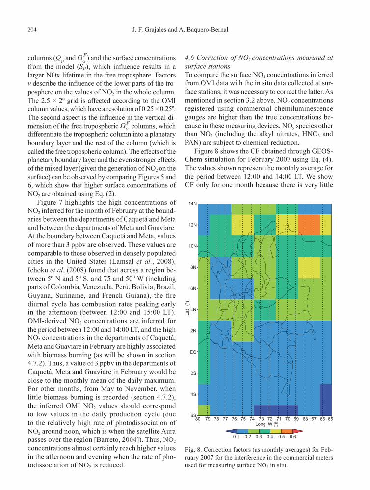
4.6 Correction of NO2 concentrations measured at surface stationsTo compare the surface NO2 concentrations inferred from OMI data with the in situ data collected at sur-face stations, it was necessary to correct the latter. As mentioned in section 3.2 above, NO2 concentrations registered using commercial chemiluminescence gauges are higher than the true concentrations be-cause in these measuring devices, NOy species other than NO2 (including the alkyl nitrates, HNO3 and PAN) are subject to chemical reduction.

Figure 8 shows the CF obtained through GEOS-Chem simulation for February 2007 using Eq. (4). The values shown represent the monthly average for the period between 12:00 and 14:00 LT. We show CF only for one month because there is very little

0.60.50.40.30.20.1

656667686970717273747576777879Long. W (º)

Lat.

(º)

806S

4S

2S

2N

4N

6N

8N

10N

12N

14N

EQ

Fig. 8. Correction factors (as monthly averages) for Feb-ruary 2007 for the interference in the commercial meters used for measuring surface NO2 in situ.


variability from month to month. Throughout most of Colombia, the CF values range from less than 0.2 to 0.4. This finding indicates an overestimation in the NO2 reading by the molybdenum catalytic converter of between 60 and 80%, which implies that a large reservoir of NO2 is present in NOy species, such as PAN, HNO3, and alkyl nitrates. Because Colombia is located in the equatorial zone, a high level of solar radiation is present during most of the year, and this result is comparable to that reported by Lamsal et al. (2008) for North America in the summer season. Lamsal et al. (2008) found lower CF values in sum-mer, with values of approximately 0.2 being predom-inant in regions with low anthropogenic activity. This result is due primarily to the short lifetime of NO2 given the influence of solar radiation during the day, which favors the conversion of NO2 to NO following the exhaustion reaction:

NO2 + hv → NO + O3O2 (R3)

During the day, NO is present in higher levels than NO2, and during the night, the converse is true.

Another important factor that affects the value of CF is anthropogenic activity, which is related to the population density and the industrial characteristics of a region. In general, the higher the levels of an-thropogenic activity, the higher the concentrations of NOx species. In remote regions, the levels of an-thropogenic activity are lower and NOy compounds prevail. From the center of Colombia to the north (i.e., in the region with the highest anthropogenic activity), the CF values are slightly higher compared with the CF values in the southern and southeastern parts of the country (which include departments with smaller populations, such as Amazonas, Guainía, Caquetá, Putumayo, and Guaviare). The highest values for all months (between 0.4 and 0.6) occur close to the Ven-ezuelan coast, probably due to anthropogenic causes.

4.7 OMI-derived NO2 concentrations versus in situ and biomass burning data4.7.1 Comparison of OMI-derived NO2 concentra-tions and in situ concentrationsCorrelation coefficients were calculated for the com-parison of the monthly mean surface NO2 concentra-tions measured in situ with those inferred from OMI data. For each in situ data point, it was necessary to apply the correction factor in the GEOS-Chem grid

that was closest to the associated measuring station. Data were only available from seven ground stations in two cities: Bogotá (six stations) and Bucaramanga (one station). Several main cities such as Medellín (Antioquia), Pereira (Risaralda), Manizales (Caldas), and Cali (Valle del Cauca) have air quality monitoring networks; however, we could only have access to the data for Bogotá and Bucaramanga. On the other hand, cities that have air quality monitoring networks are located west of the Cordillera Oriental, so that in much of the country, no surface stations exist from which air quality data can be obtained to study the sources and transport mechanisms of pollutants in Colombia.

The stations located and used in Bogotá are IDRD, MAVDT, Fontibón, Las Ferias, Puente Aranda, and Suba. The station located and used in Bucaramanga is Centro. The number of data points used simulta-neously for inferred monthly NO2 concentrations and measuring stations in Bogotá and Bucaramanga is presented in Table II. As can be observed in this table, certain averages were calculated using only one simultaneous data point, and in the best case, some averages were calculated using 20 simultaneous data points. Since Bogotá has an area of 1600 km2, two OMI grid cells at the resolution 0.5 × 0.5º were used to compare with the station data. The location of the midpoint of each grid cell is shown in Table III.

Monthly averages and correlations for stations in Bucaramanga and Bogotá are presented in Table IV. The in situ data that are most highly correlated with the OMI inferred data are those from the Puente Aranda, IDRD and MAVDT stations. Data from these three stations yield Pearson coefficients of 0.91, 0.56 and 0.55 and Spearman coefficients of 0.81, 0.55 and 0.78, respectively. The stations with the highest annual mean are Puente Aranda, MAVDT and Las Ferias, in that order. It is noted that the Puente Aranda station is located in the second-biggest industrial zone in Colombia, which could mean that concentration of polluting agents, in particular NO2, could be ho-mogeneous in the surrounding area represented by the corresponding OMI grid cell (Bogotá 1), so that Puente Aranda could have the best local background measurements relative to the other stations.

Figures 9-11 show the monthly means of NO2 concentrations from the stations in Bogotá and Bucar-amanga and the corresponding inferred OMI values. The NO2 concentrations inferred from OMI data for


Colombia are similar to those found by Lamsal et al. (2008) in the U.S. for the summer season. These au-thors reported NO2 concentrations of 0.1 ppbv in rural regions and between 2 and 3 ppbv in urban areas. Since the measurements at the stations are at surface level, they do not reflect the influence of either the mixed layer or the horizontal atmospheric movements, both of which serve to mix atmospheric pollutants. Thus, inferred OMI NO2 concentration tends to be lower than point measurements reported at the corresponding sta-tions. Therefore, the values for the stations reported in Figures 9-11 could have overestimations even though they correspond to corrected data according to the CF obtained from GEOS-Chem (section 4.6). Such CFs are influenced by the interferences caused mainly by NOy species such as PAN, alkyl nitrates and HNO3 (see Eq. 4). Thus, it can be expected that, despite the correction, surface NO2 concentrations from the sta-tions are still overestimated. It is therefore desirable to determine the conversion rates of interfering NOy species. The conversion of HNO3 is not easy to resolve and depends on the measuring equipment, as noted by Lamsal et al. (2008), who reported a value of 35%. In the cases of PAN and alkyl nitrates, conversion to more stable compounds is expected (Steinbacher et al., 2007). On the other hand, a main reason for the underestimation of satellite-inferred concentrations is the limited sensitivity of the remote sensing instrument close to the surface.

It should also be noted that our data validation pro-cess was limited because a high layer of cloud cover is usually present over the mountainous regions. This cloud cover impedes the measurement of NO2 col-umns in the visible spectrum (section 2.1) and as can be observed on the map in Figure 12, the lack of data for the Andean region (departments of Nariño, Cauca, Valle del Cauca, Huila, Tolima, Risaralda, Quindío, Cundinamarca, Antioquia, Boyacá, Santander and Norte de Santander) is considerable. The scarcity of data for the mountainous regions is not unique to 2007. Similar patterns are evident for the years 2008 Ta

ble

II. N

umbe

r of d

aily

dat

a po

ints

ava

ilabl

e si

mul

tane

ousl

y fo

r cal

cula

tion

of th

e m

onth

ly a

vera

ge N

O2 c

once

ntra

tions

from

the

OM

I and

from

the

surf

ace

stat

ions

in B

ogot

á an

d B

ucar

aman

ga.

Janu

ary

Febr

uary

M

arch

Apr

ilM

ayJu

neJu

lyA

ugus

tSe

ptem

ber

Oct

ober

Nov

embe

rD

ecem

ber

Tota

l

OM

I at B

ogot

á 1

1015

21

25

72

48

02

58ID

RD

1015

21

25

72

48

02

58O

MI a

t Bog

otá

112

202

22

57

24

78

374

MAV

DT

1220

22

25

72

47

83

74O

MI a

t Bog

otá

112

202

22

57

25

82

067

Font

ibón

1220

22

25

72

58

20

67O

MI a

t Bog

otá

110

202

22

30

06

89

264

Las F

eria

s10

202

22

30

06

89

264

OM

I at B

ogot

á 1

619

22

25

72

68

93

71Pu

ente

Ara

nda

619

22

25

72

68

93

71O

MI a

t Bog

otá

26

162

02

23

22

55

045

Suba

616

20

22

32

25

50

45O

MI a

t Buc

aram

anga

1120

22

25

72

68

83

76C

entro

1120

22

25

72

68

83

76

Table III. Location of the midpoint of the two grid cells used to compare with the station data at Bogotá.

Longitude W(º) Latitude N(º)

Bogotá 1 74.125 4.625Bogotá 2 74.125 4.875Bucaramanga 73.125 7.125


Tabl

e IV

. Mon

thly

ave

rage

surf

ace

conc

entra

tions

of N

O2 (

in p

pbv)

infe

rred

from

OM

I dat

a us

ing

Eq. (

2) a

nd c

orre

cted

mea

sure

men

ts a

t the

stat

ions

in B

ogot

á an

d B

ucar

aman

ga.

Janu

ary

Febr

uary

M

arch

Apr

ilM

ayJu

neJu

lyA

ugus

tSe

ptem

ber

Oct

ober

Nov

embe

rD

ecem

ber

OM

I inf

erre

d at

Bog

otá

1 (I

DR

D)

0.59

0.54

1.07

0.16

0.08

0.44

0.27

0.13

0.21

0.32

0.45

IDR

D S

tatio

n2.

273.

383.

022.

810.

640.

370.

500.

501.

851.

462.

16

Pear

son

corr

elat

ion

0.56

Spea

rman

n co

rrel

atio

n0.

55

OM

I inf

erre

d at

Bog

otá

1 (M

AVD

T)0.

540.

621.

071.

270.

080.

440.

270.

130.

150.

330.

620.

68M

AVD

T St

atio

n5.

6811

.63

9.67

4.21

1.92

2.03

1.46

1.11

1.33

2.72

2.23

2.50

Pear

son

corr

elat

ion

0.55

Spea

rman

n co

rrel

atio

n0.

78

OM

I inf

erre

d at

Bog

otá

1 (F

ontib

ón)

0.54

0.62

1.07

1.27

0.08

0.44

0.27

0.13

0.17

0.32

0.44

Font

ibon

Sta

tion

2.12

2.36

2.66

2.26

2.19

1.90

1.70

2.11

2.91

3.08

3.13

Pear

son

corr

elat

ion

0.04

Spea

rman

n co

rrel

atio

n0.

16

OM

I inf

erre

d at

Bog

otá

1 (L

as F

eria

s)0.

630.

621.

071.

270.

080.

510.

140.

320.

590.

67La

s Fer

ias S

tatio

n2.

953.

583.

302.

260.

780.

623.

324.

774.

614.

36

Pear

son

corr

elat

ion

0.10

Spea

rman

n co

rrel

atio

n–0

.01

OM

I inf

erre

d at

Bog

otá

1 (P

uent

e A

rand

a)0.

700.

601.

071.

270.

080.

440.

270.

130.

140.

320.

590.

68

Puen

te A

rand

a St

atio

n4.

404.

605.

326.

003.

743.

683.

553.

133.

764.

584.

464.

80

Pear

son

corr

elat

ion

0.91

Spea

rman

n co

rrel

atio

n0.

81

OM

I inf

erre

d at

Bog

otá

2 (S

uba)

0.39

0.61

0.39

0.06

0.39

0.81

0.15

0.33

0.26

0.60

Suba

Sta

tion

2.33

0.73

0.58

0.10

0.65

1.17

1.65

1.50

3.19

3.06

Pear

son

corr

elat

ion

0.10

Spea

rman

n co

rrel

atio

n0.

04

OM

I inf

erre

d at

Buc

aram

anga

(C

entro

)0.

580.

621.

071.

270.

080.

440.

270.

130.

140.

320.

610.

68

Cen

tro S

tatio

n1.

771.

742.

231.

582.

141.

932.

052.

095.

063.

934.

234.

69

Pear

son

corr

elat

ion

–0.2

3Sp

earm

ann

corr

elat

ion

–0.2

4


1 2 3 4 5 6 7 8 9 10 11 120.0

2.0

4.0

6.0

8.0

10.0

12.0

14.0IDRD StationMAVDT StationPuente Aranda StationFontibón StationLas Ferias StationOMI inferred at Bogotá 1 (IDRD)OMI inferred at Bogotá 1 (MAVDT)OMI inferred at Bogotá 1 (Puente Aranda)OMI inferred at Bogotá 1 (Fontibón)OMI inferred at Bogotá 1 (Las Ferias)

Month

NO

2 co

ncen

tratio

n (p

pbv)

Fig. 9. Monthly average surface concentrations of NO2 (in ppbv) at Bogotá 1 inferred from OMI data using Eq. (2) and from corrected measurements at the IDRD, MAVDT and Puente Aranda, Fontibón and Las Ferias stations, which are located in Bogotá. All the curves correspond to values in Table IV.

1 2 3 4 5 6 7 8 9 10 11 120.0

0.5

1.0

1.5

2.0

2.5

3.0

3.5

Suba Station OMI inferred at Bogotá 2Month

NO

2 co

ncen

tratio

n (p

pbv)

Fig. 10. Monthly average surface concentrations of NO2 (in ppbv) at Bogotá 2 inferred from OMI data using Eq. (2) and from corrected measurements at Suba station, which is located in Bogotá.

1 2 3 4 5 6 7 8 9 10 11 120.0

1.0

2.0

3.0

4.0

5.0

6.0

OMI inferred at Bucaramanga Centro StationMonth

NO

2 co

ncen

tratio

n (p

pbv)

Fig. 11. Monthly average surface concentrations of NO2 (in ppbv) at Bucaramanga inferred from OMI data using Eq. (2) and from corrected measurements at Centro station, which is located in Bucaramanga.


and 2009 (not shown). Unfortunately, the surface measurement stations available to provide data use-ful for validation are located in a mountainous and cloudy area. Six of the seven stations are located in Bogotá, which is located in the Andean region and has an elevation of 2600 m. The seventh station is located in Bucaramanga, which is also located in the Andean region and has an elevation of 959 m. The extension of the network of surface measurement stations to both remote and new urban areas would enable more comprehensive measurement of back-ground concentrations of NO2 and would facilitate a more complete validation throughout Colombia.

4.7.2 Estimated NO2 surface concentration vs. MACC Fire Radiative PowerFire radiative power (FRP) determines the burning rate of biomass (living and dead vegetation). The Global Fire Assimilation System (GFASv1.0) calcu-lates biomass-burning emissions by assimilating FRP observations from the MODIS instrument onboard

the Terra and Aqua satellites (Kaiser et al., 2012). We used the FRP data from the Daily Wildfire Emissions product provided by the Monitoring Atmospheric Composition & Climate (MACC) project (available at http://macc.iek.fz-juelich.de/data/compressed/orig/MACC_Daily_Wildfire_Emissions/). FRP daily data has a horizontal spatial resolution of 0.5 × 0.5º (latitude × longitude), and has been produced since 2003 to the present.

Figure 13 shows monthly means of FRP for 2007. It can be noted that a high amount of biomass was burned in Colombia in February (and also in January and March [not shown]), while biomass burning was scarce in the months after. Figure 14 shows maps of correlation between FRP and OMI-de-rived NO2 surface concentration estimated in section 4.5. The biggest number of grid points with high cor-relation values (> 0.5) is observed for February (and also in January and March [not shown]), especially in Vichada, Meta, Guaviare, Caquetá, and the western part of Venezuela, regions where the prevailing biome is humid tropical forest. This implies that the high NO2 concentrations in Figure 7 in these regions are mostly attributable to biomass burning. The correlations are low in the months after. In Cesar, Magdalena, Bolívar, and La Guajira, where the prevailing biome is trop-ical dry forest, there are intermediate values of FRP (Fig. 13). The correlation values between FRP and the estimated NO2 surface concentration (Fig. 14) in these regions suggest that the NO2 concentrations are partially due to biomass burning and partially due to industrial NO2 generating processes.

5. Conclusions1. There is an overestimation of OMI columns in remote regions. We propose that on remote regions, where the density of OMI NO2 columns is expected to be very low, the amount of 0.4 × 1015 molecules/cm2

should be subtracted.2. The inferred NO2 concentration values are relative-ly low (between 0.01 and 0.5 ppbv) throughout most of the country. However, relatively high concentra-tions (between 3 and 4 ppbv) occur in the departments of Caquetá and Meta in February. A main reason for the underestimation of satellite-inferred concentra-tions is the limited sensitivity of the remote sensing instrument close to the surface.3. The comparison of NO2 concentrations inferred from OMI data and those based on ground station

12N

10N

8N

Lat.

(º)

6N

4N

2N

EQ

2S

4S

79 78 77 76 75Long. W (º)

74 73 72 71 70 69 68 67 66

360

330

300

270

240

210

180

150

120

90

60

30

Fig. 12. Number of missing data points in the OMNO2e product for 2007.


measurements from the stations Puente Aranda, IDRD and MAVDT in Bogotá yields Pearson correla-tion coefficients of 0.91, 0.56 and 0.55 and Spearman coefficients of 0.81, 0.55 and 0.78, respectively.4. The comparison of the NO2 concentrations in-ferred from OMI data and FRP yields high correla-tion coefficients in areas where the concentrations are high. These areas are tropical rainforests. This indicates that these high NO2 concentrations are due to biomass burning, which includes the human-ini-tiated burning of vegetation for land clearing and land use change as well as natural, lightning-induced

fires. In areas with correlations between 0.4 and 0.7 (located in western Venezuela and central and north-ern Colombia during February), NO2 concentrations can be partially associated with biomass burning and partially with other processes such as transport of NO2 or its precursors from other regions, burn-ing of fossil fuels by the oil industry, and diverse industrial processes.

AcknowledgmentsThis work is supported by the Proyecto Piloto Na-cional de Adaptación al Cambio Climático (INAP,

February April June


Lat.

(º)

4S

2S

2N

4N

6N

8N

10N

12N

EQ

Lat.

(º)

4S

2S

2N

4N

6N

8N

10N

12N

EQ

0.2

0.10.05

0.01

0.005

0.001

0.2

0.10.05

0.01

0.005

0.001


Fig. 13. Monthly means of FRP for 2007 in W/m2. Only the maps for even months are shown.


National Pilot Project on Adaptation to Climate Change) and the Dirección de Investigaciones Sede Bogotá (DIB, Directorate of Research of Bogotá) of the Universidad Nacional de Colombia through the Convocatoria Nacional de Investigación y Creación Artística 2010-2012 (National Call for Research and Artistic Creation 2010-2012).

ReferencesAckermann-Liebrich U., 1997. Lung function and long-

term exposure to air pollutants in Switzerland: Study on air pollution and lung diseases in adults (SAPALDIA) team. Am. J. Respir. Crit. Care Med. 155, 122-129.

Barreto P. L. R., 2004. Estudio de la contaminación por niebla fotoquímica con relación a las emisiones y el

February April June


Lat.

(º)

4S

2S

2N

4N

6N

8N

10N

12N

EQ

Lat.

(º)

4S

79 78 77 76 75 74 73 72 71 70 69 68 67 66 65 79 78 77 76 75 74 73 72 71 70 69 68 67 66 65 79 78 77 76 75 74 73 72 71 70 69 68 67 66 65Long. W (º)

2S

2N

4N

6N

8N

10N

12N

EQ

Long. W (º) Long. W (º)

0.90.8

0.7

0.6

0.5

0.4

–0.4

0.3

–0.3

0.2

–0.2

0.1

–0.1

0

0.90.8

0.7

0.6

0.5

0.4

–0.4

0.3

–0.3

0.2

–0.2

0.1

–0.1

0

Fig. 14. Correlation maps between inferred NO2 surface concentration and FRP interpolated to the 0.5 × 0.5º resolution. For these correlation maps a minimum number of non-missing daily values for each variable in each grid point was taken into account; this number is equal to 12. Correlations equal to or higher than 0.5 are statistically significant at the 90% level. Blank grid boxes represent either: (1) that the requirement of having a minimum of 12 daily non-missing simultaneous values is not met, or (2) that FRP daily values are equal to zero for the whole year. The second situation is to be found, e.g., over the sea. Only the maps for even months are shown.


comportamiento de la atmósfera en la ciudad de Bo-gotá. Tesis de maestría en Meteorología, Facultad de Ciencias, Universidad Nacional de Colombia.

Bedoya V. J., 1981. Fuentes contaminantes del aire en el valle de Aburrá. Revista AINSA 1, 66-77.

Benavides B. H. O., 2003. Pronóstico de la concentración de material particulado por chimeneas industriales en Bogotá. Tesis de maestría en Meteorología, Facultad de Ciencias, Universidad Nacional de Colombia.

Bey I., D. Jacob, R. M. Yantosca, J. A. Logan, B. D. Field, A. M. Fiore, Q. Li, H. Y. Liu, L. J. Mickley and M. G. Schultz, 2001. Global modeling of tropospheric chem-istry with assimilated meteorology: Model description and evaluation. J. Geophys. Res. 106, 23073-23096.

Boersma K. F., H. J. Eskes, J. P. Veefkind, E. J. Brinksma, R. J. Van Der A, M. Sneep, G. H. J. Van Den Oord, P. F. Levelt, P. Stammes, J. F. Gleason and E. J. Bucsela, 2007. Near-real time retrieval of tropospheric NO2 from OMI. Atm. Chem. Phys. 7, 2103-2118.

Boersma K. F., D. J. Jacob, E. J. Bucsela, A. E. Perring, R. Dirksen, R. J. van der A, R. M. Yantosca, R. J. Park, M. O. Wenig, T. H. Bertram and R. C. Cohen, 2008. Validation of OMI tropospheric NO2 observations during INTEX-B and application to constrain NOx

emissions over the eastern United States and Mex-ico. Atmos. Environ. 42, 4480-4497, doi:10.1016/j.atmosenv.2008.02.004.

Boersma K. F., R. Braak and R. J. van der A, 2011. Dutch OMI NO2 (DOMINO) data product v2.0 HE5 data file user manual.

Bond T. C., E. Bhardwaj, R. Dong, R. Jogani, S. Jung, C. Roden, D. G. Streets and N. M. Trautmann, 2007. Historical emissions of black and organic carbon aerosol from energy related combustion, 1850-2000. Global Biogeochem. Cy. 21, GB2018, doi:10.1029/2006GB002840.

Bucsela E. J., E. A. Celarier, M. O. Wenig, J. F. Gleason, J. P. Veefkind, K. F. Boersma and E. J. Brinksma, 2006. Algorithm for NO2 vertical column retrieval from the ozone monitoring instrument. IEEE T. on Geosci. Re-mote 44, doi:10.1109/TGRS.2005.863715.

Bucsela E. J., A. E. Perring, R. C. Cohen, K. F. Boers-ma, E. A. Celarier, J. F. Gleason, M. O. Wenig, T. H. Bertram, P. J. Wooldridge, R. Dirksen and J. P. Veefkind, 2008. Comparison of tropospheric NO2 in situ aircraft measurements with near-real-time and standard product data from the Ozone Moni-toring Instrument. J. Geophys. Res. 113, D16S31. doi:10.1029/2007JD008838.

Celarier E. A., E. J. Brinksma, J. F. Gleason, J. P. Veef-kind, A. Cede, J. R. Herman, D. Ionov, F. Goutail, J.-P. Pommereau, J.-C. Lambert, M. van Roozendael, G. Pinardi, F. Wittrock, A. Schönhardt, A. Richter, O. W. Ibrahim, T. Wagner, B. Bojkov, G. Mount, E. Spinei, C. M. Chen, T. J. Pongetti, S. P. Sander, E. J. Bucsela, M. O. Wenig, D. P. J. Swart, H. Volten, M. Kroon and P. F. Levelt, 2008. Validation of ozone monitoring in-strument nitrogen dioxide columns. J. Geophys. Res. 113, D15S15, doi:10.1029/2007JD008908.

Dunlea E. J., S. C. Herndon, D. D. Nelson, R. M. Volkamer, F. San Martini, P. M. Sheehy, M. S. Zahniser, J. H. Shorter, J. C. Wormhoudt, B. K. Lamb, E. J. Allwine, J. S. Gaffney, N. A. Marley, M. Grutter, C. Márquez, S. Blanco, B. Cárdenas, A. Retama, C. R. Ramos Vil-legas, C. E. Kolb, L. T. Molina and M. J. Molina, 2007. Evaluation of nitrogen dioxide chemiluminescence monitors in a polluted urban environment. Atmos. Chem. Phys. 7, 2691-2704.

Ellis E. C., 1975. Technical assistance document for the chemiluminescence measurement of nitrogen diox-ide. Technical report. Environmental Monitoring and Support Laboratory, U.S. Environmental Protection Agency. EPA-600/4-75-003.

Evans M. J., A. Fiore and D. J. Jacob, 2003. The GEOS-Chem chemical mechanism version 5-07-8. Harvard University, Cambridge. Available at: http://acmg.seas.harvard.edu/geos/wiki_docs/chemistry/geoschem_mech.pdf (last accessed on March 10, 2014.

Gass J., 2012. The GEOS-5 System. NASA, Global Modeling and Assimilation Office. Available at: http://gmao.gsfc.nasa.gov/systems/geos5/ (last accessed on March 10, 2014).

Gauderman W. J., 2000. Association between air pollu-tion and lung function growth in southern California children. Am. J. Respir. Crit. Care Med. 162, 1383-1390.

Gauderman W. J., 2002. Association between air pollu-tion and lung function growth in southern California children: Results from a second cohort. Am. J. Respir. Crit. Care Med. 166, 76-84.

Grosjean D. and J. Harrison, 1985. Response of chemi-luminescence NOx analyzers and ultraviolet ozone analyzers to organic air pollutants. Environ. Sci. and Technol. 19, 862-865.

Ichoku C., L. Giglio, M. J. Wooster and L. A. Remer, 2008. Global characterization of biomass-burning patterns using satellite measurements of fire radiative energy. Remote Sens. Environ. 112, 2950-2962.


Jacob D., 1999. Introduction to atmospheric chemistry. 11.4. Global budget of the nitrogen oxides. Princeton University Press, 211-215.

Jiménez P. R., 2004. Development and application of UV-visible and mid-IR differential absorption spec-troscopy techniques for pollutant trace gas monitoring. Ph.D. thesis no. 2944. École Polytechnique Fédérale de Lausanne, France, 230 pp.

Jones P. W., 1999. First and second order conservative remapping schemes for grids in spherical coordinates. Mon. Weather Rev. 127, 2204-2210.

Kaiser J. W., A. Heil, M. O. Andreae, A. Benedetti, N. Chu-barova, L. Jones, J.-J. Morcrette, M. Razinger, M. G. Schultz, M. Suttie and G. R. van der Werf, 2012. Biomass burning emissions estimated with a global fire assimi-lation system based on observed fire radiative power. Biogeosciences 9, 527-554, doi:10.5194/bg-9-527-2012.

Kempler S. J., 2010. OMI data products and data access. NASA, Godard Earth Sciences Sata and Information Services Center. Available at: http://disc.sci.gsfc.nasa.gov/Aura/overview/data-holdings/OMI/index.shtml (last accessed on November 20, 2012).

Lacouture C. J. A., 1979. Estudio de la contaminación por ozono, dióxido de nitrógeno y formaldehído como agentes de contaminación atmosférica. Tesis en Ingenieria Civil, Facultad de Ingeniería. Pontificia Universidad Javeriana, Bogotá, Colombia.

Lamsal L. N., R. V. Martin, A. van Donkelaar, M. Stein-bacher, E. A. Celarier, E. Bucsela, E. J. Dunlea and J. P. Pinto, 2008. Ground-level nitrogen dioxide con-centrations inferred from the satellite-borne ozone monitoring instrument. J. Geophys. Res. 113, D16308, doi:10.1029/2007JD009235.

Le Sager P., B. Yantosca and C. Carouge, 2008. GEOS-Chem v8–02–01 online user’s guide. Appendix 3: Vertical grids. Atmospheric Chemistry Modeling Group, School of Engineering and Applied Sciences, Harvard University. Available at: http://acmg.seas.harvard.edu/geos/doc/archive/man.v8-02-01/index.html (last accessed on March 10, 2014).

Martin R. V., D. D. Parrish, T. B. Ryerson, D. K. Nicks Jr., K. Chance, T. P. Kurosu, D. J. Jacob, E. D. Sturges, A. Fried and B. P. Wert, 2004. Evaluation of GOME satellite measurements of tropospheric NO2 and HCHO using regional data from aircraft campaigns in the southeastern United States. J. Geophys. Res. 109, D24307, doi:10.1029/2004JD004869.

Martin R., C. E. Sioris, K. Chance, T. Ryerson, T. H. Bertram, P. J. Wooldridge, R. C. Cohen, J. A. Neu-

man, A. Swanson and F. Flocke, 2006. Evaluation of space-based constraints on global nitrogen oxide emissions with regional aircraft measurements over and downwind of eastern North America. J. Geophys. Res. 111, D15308. doi:10.1029/2005JD006680.

Olivier J. G. J. and J. J. M. Berdowski, 2001. Global emissions sources and sinks. In: The climate system (J. Berdowski, R. Guicherit and B. J. Heij, Eds.). A. A. Balkema Publishers/Swets & Zeitlinger Publishers, Lisse, The Netherlands, 33-50.

OMI Team, 2009. Ozone monitoring instrument (OMI) data user’s guide. OMI-DUG-3.0. Available at: http://views.cira.colostate.edu/data/Documents/Guidelines/README.OMI_DUG.pdf (last accessed on March 10, 2014).

Oviedo T. B. E., 2009. Análisis del efecto del cambio climático en la dispersión de ozono y material particulado en Bogotá. Tesis de maestría en Meteo-rología. Facultad de Ciencias, Universidad Nacional de Colombia.

Panella M., V. Tommasini, M. Binotti, L. Palin and G. Bona, 2000. Monitoring nitrogen dioxide and its effects on asthmatic patients: Two different strategies compared. Environ. Monitoring Assess. 63, 447-458.

Rienecker M. M., M. J. Suárez, R. Todling, J. Bacmeister, L. Takacs, H.-C. Liu, W. Gu, M. Sienkiewicz, R. D. Koster, R. Gelaro, I. Stajner and E. Nielsen, 2008. The GEOS-5 Data Assimilation System – Documentation of Versions 5.0.1, 5.1.0, and 5.2.0. NASA technical report series on global modeling and data assimilation 104606, V27.

Ruiz M. J. F., 2002. Simulación de la contaminación atmosférica generada por fuentes móviles en Bogotá. Tesis de maestría en Meteorología, Facultad de Cien-cias, Universidad Nacional de Colombia.

Sauvage, B., R. V. Martin, A. van Donkelaar and J. R. Ziemke, 2007. Quantification of the factors controlling tropical tropospheric ozone and the south Atlantic maximum. J. Geophys. Res. 112, D11309, doi:10.1029/2006JD008008.

Schindler C., U. Ackermann-Liebrich, P. Leuenberger, C. Monn, R. Rapp, G. Bolognini, J.-P. Bongard, O. Brändli, G. Domenighetti, W. Karrer, R. Keller, T. G. Medici, A. P. Perruchoud, M. H. Schöni, J.-M. Tschopp, B. Villiger, J.-P. Zellweger and the SAPALDIA Team, 1998. Associations between lung function and estimated average exposure to NO2 in eight areas of Switzerland. The SAPALDIA Team. Swiss study of air pollution and lung diseases in adults. Epidemiology 9, 405-411.


Smith B. J., M. Nitschke, L. S. Pilotto, R. E. Ruffin, D. L. Pisaniello and K. J. Willson, 2000. Health effects of daily indoor nitrogen dioxide exposure in people with asthma. Eur. Respir. J. 16, 879-885.

Steinbacher M., C. Zellweger, B. Schwarzenbach, S. Bugmann, B. Buchmann, C. Ordoñez, A. S. H. Prevot and C. Hueglin, 2007. Nitrogen oxides measurements at rural sites in Switzerland: Bias of conventional measurement techniques. J. Geophys. Res., D11307, doi:10.1029/ 2006JD007971.

Torres O., R. Decae, J. P. Veefkind and G. de Leeuw, 2002. OMI aerosol retrieval algorithm. In: OMI algorithm theoretical basis document: Clouds, aerosols, and sur-face UV irradiance (P. Stammes, Ed.). OMI-ATBD-03,

vol. 3, version 2. NASA Goddard Space Flight Cen-ter, Greenbelt, Maryland, 47-71. Available at: http://ebookbrowsee.net/atbd-omi-03-pdf-d489054159 (last accessed on March 10 2014).

Van der Werf G. R., D. C. Morton, R. S. DeFries, L. Giglio, J. T. Randerson, G. J. Collatz and P. S. Ka-sibhatla, 2009. Estimates of fire emissions from an active deforestation region in the southern Amazon based on satellite data and biogeochemical modelling. Biogeosciences 6, 235-249.

Wang Y., D. J. Jacob and J. A. Logan, 1998. Global simulation of tropospheric O3-NOx-hydrocarbon chemistry – 1. Model formulation. J. Geophys. Res. 103, 10713-10726.