inference in generalized linear models with applicationsschniter/pdf/byrne_diss.pdf · inference in...

Inference in Generalized Linear Models with Applications

Dissertation

Presented in Partial Fulfillment of the Requirements for the DegreeDoctor of Philosophy in the Graduate School of The Ohio State

University

By

Evan Byrne, B.S., M.S.

Graduate Program in Electrical and Computer Engineering

The Ohio State University

2019

Dissertation Committee:

Dr. Philip Schniter, Advisor

Dr. Lee C. Potter

Dr. Kiryung Lee

c© Copyright by

Evan Byrne

2019

Abstract

Inference involving the generalized linear model is an important problem in signal

processing and machine learning. In the first part of this dissertation, we consider

two problems involving the generalized linear model. Specifically, we consider sparse

multinomial logistic regression (SMLR) and sketched clustering, which in the context

of machine learning are forms of supervised and unsupervised learning, respectively.

Conventional approaches to these problems fit the parameters of the model to the data

by minimizing some regularized loss function between the model and data, which typ-

ically is performed by an iterative gradient-based algorithm. While these methods

generally work, they may suffer from various issues such as slow convergence or get-

ting stuck in a sub-optimal solution. Slow convergence is particularly detrimental

when applied to modern datasets, which may contain upwards of millions of sam-

ple points. We take an alternate inference approach based on approximate message

passing, rather than optimization. In particular, we apply the hybrid generalized ap-

proximate message passing (HyGAMP) algorithm to both of these problems in order

to learn the underlying parameters of interest. The HyGAMP algorithm approximates

the sum-product or min-sum loopy belief propagation algorithms, which approximate

minimum mean squared error (MMSE) or maximum a posteriori (MAP) estimation,

respectively, of the unknown parameters of interest. We first apply the MMSE and

ii

MAP forms of the HyGAMP algorithm to the SMLR problem. Next, we apply a sim-

plified form of HyGAMP (SHyGAMP) to SMLR, where we show through numerical

experiments that our approach meets or exceeds the performance of state-of-the-art

SMLR algorithms with respect to classification accuracy and algorithm training time

(i.e., computational efficiency). We then apply the MMSE-SHyGAMP algorithm to

the sketched clustering problem, where we also show through numerical experiments

that our approach exceeds the performance of other state-of-the-art sketched clus-

tering algorithms with respect to clustering accuracy and computational efficiency.

We also show our approach has better clustering accuracy and better computational

efficiency than the widely used K-means++ algorithm in some regimes.

Finally, we study the problem of adaptive detection from quantized measurements.

We focus on the case of strong, but low-rank interference, which is motivated by wire-

less communications applications for the military, where the receiver is experiencing

strong jamming from a small number of sources in a time-invariant channel. In this

scenario, the receiver requires many antennas to effectively null out the interference,

but this comes at the cost of increased hardware complexity and increased volume of

data. Using highly quantized measurements is one method of reducing the complexity

of the hardware and the volume of data, but it is unknown how this method affects

detection performance. We first investigate the effect of quantized measurements on

existing unquantized detection algorithms. We observe that unquantized detection

algorithms applied to quantized measurements lack the ability to null arbitrarily large

interference, despite being able to null arbitrarily large interference when applied to

unquantized measurements. We then derive a generalized likelihood ratio test for the

quantized measurement model, which again gives rise to a generalized bilinear model.

iii

Via simulation, we empirically observe the quantized algorithm only offers a fraction

of a decibel improvement in equivalent SNR relative to unquantized algorithms. We

then evaluate alternative techniques to address the performance loss due to quan-

tized measurements, including a novel analog pre-whitening using digitally controlled

phase-shifters. In simulation, we observe that the new technique shows up to 8 dB

improvement in equivalent SNR.

iv

Acknowledgments

Many people deserve thanks for assisting me in the process of completing this dis-

sertation. First and foremost I must thank my advisor Phil Schniter for contributing

a significant amount of time and effort towards mentoring me and for guiding my

research with helpful insights and advise. I also want to thank many ECE faculty,

particularly Lee Potter, for serving on my numerous committees and for teaching ex-

citing and useful courses. I am also very grateful towards Adam Margetts, who served

as a dedicated mentor and collaborator for much of my dissertation, and towards MIT

Lincoln Laboratory for financially supporting a large portion of my research.

Other people in the department helped as well. Jeri McMichael and Tricia Tooth-

man were always friendly to talk to, interested in my progress, and provided valuable

help in scheduling and other areas. The other IPS students, including Jeremy Vila,

Justin Ziniel, Mark Borgerding, Mike Riedl, Adam Rich, You Han, Tarek Abdal-

Rahmen, Subrata Sarkar, Ted Reehorst, and Antoine Chatalic provided a welcoming

community, support and collaboration.

Finally, I am very thankful for my family and friends, who supported and encour-

aged me the entire way.

v

Vita

December 2012 . . . . . . . . . . . . . . . . . . . . . . . . . . . . . B.S. Electrical and Computer Engi-neering, The Ohio State University

August 2015 . . . . . . . . . . . . . . . . . . . . . . . . . . . . . . . .M.S. Electrical and Computer Engi-neering, The Ohio State University

2013-present . . . . . . . . . . . . . . . . . . . . . . . . . . . . . . . .Graduate Research Assistant,The Ohio State University

Publications

E. Byrne and P. Schniter, “Sparse Multinomial Logistic Regression via ApproximateMessage Passing,” IEEE Transactions on Signal Processing, vol. 64, no. 21, pp.

5485-5498, Nov. 2016.

S. Rangan, A. K. Fletcher, V. K. Goyal, E. Byrne, and P. Schniter, “Hybrid Approx-imate Message Passing,” IEEE Transactions on Signal Processing, vol. 65, no. 17,

pp. 4577-4592, Sep. 2017.

E. Byrne, R. Gribonval, and P. Schniter, “Sketched Clustering via Hybrid Approxi-mate Message Passing,” Proc. Asilomar Conf. on Signals, Systems, and Computers

(Pacific Grove, CA), Nov. 2017.

P. Schniter and E. Byrne, “Adaptive Detection of Structured Signals in Low-RankInterference,” IEEE Transactions on Signal Processing, accepted.

E. Byrne, A. Chatalic, R. Gribonval, and P. Schniter, “Sketched Clustering via HybridApproximate Message Passing,” in review.

vi

Fields of Study

Major Field: Electrical and Computer Engineering

Studies in:

Machine LearningSignal Processing

vii

Table of Contents

Page

Abstract . . . . . . . . . . . . . . . . . . . . . . . . . . . . . . . . . . . . . . . ii

Acknowledgments . . . . . . . . . . . . . . . . . . . . . . . . . . . . . . . . . . v

Vita . . . . . . . . . . . . . . . . . . . . . . . . . . . . . . . . . . . . . . . . . vi

List of Figures . . . . . . . . . . . . . . . . . . . . . . . . . . . . . . . . . . . ix

List of Tables . . . . . . . . . . . . . . . . . . . . . . . . . . . . . . . . . . . . x

1. Introduction . . . . . . . . . . . . . . . . . . . . . . . . . . . . . . . . . . 1

1.1 Introduction to Generalized Linear Models . . . . . . . . . . . . . . 31.1.1 The Standard Linear Model . . . . . . . . . . . . . . . . . . 3

1.1.2 The Generalized Linear Model . . . . . . . . . . . . . . . . 4

1.1.3 The Generalized Bilinear Model . . . . . . . . . . . . . . . . 61.1.4 Summary . . . . . . . . . . . . . . . . . . . . . . . . . . . . 7

1.2 Introduction to Approximate Message Passing . . . . . . . . . . . . 71.3 Outline and Contributions . . . . . . . . . . . . . . . . . . . . . . . 9

1.3.1 The HyGAMP Algorithm . . . . . . . . . . . . . . . . . . . 101.3.2 Sparse Multinomial Logistic Regression . . . . . . . . . . . 10

1.3.3 Sketched Clustering . . . . . . . . . . . . . . . . . . . . . . 111.3.4 Adaptive Detection from Quantized Measurements . . . . . 12

2. The Hybrid-GAMP Algorithm . . . . . . . . . . . . . . . . . . . . . . . . 13

2.1 Model . . . . . . . . . . . . . . . . . . . . . . . . . . . . . . . . . . 132.2 The HyGAMP Algorithm . . . . . . . . . . . . . . . . . . . . . . . 14

2.3 Simplified HyGAMP . . . . . . . . . . . . . . . . . . . . . . . . . 152.4 Scalar-variance Approximation . . . . . . . . . . . . . . . . . . . . 17

2.5 Conclusion . . . . . . . . . . . . . . . . . . . . . . . . . . . . . . . 18

viii

3. Sparse Multinomial Logistic Regression via Approximate Message Passing 19

3.1 Introduction . . . . . . . . . . . . . . . . . . . . . . . . . . . . . . 193.1.1 Multinomial logistic regression . . . . . . . . . . . . . . . . 20

3.1.2 Existing methods . . . . . . . . . . . . . . . . . . . . . . . . 213.1.3 Contributions . . . . . . . . . . . . . . . . . . . . . . . . . . 22

3.2 HyGAMP for Multiclass Classification . . . . . . . . . . . . . . . . 243.2.1 Classification via sum-product HyGAMP . . . . . . . . . . 25

3.2.2 Classification via min-sum HyGAMP . . . . . . . . . . . . . 283.2.3 Implementation of sum-product HyGAMP . . . . . . . . . . 29

3.2.4 Implementation of min-sum HyGAMP . . . . . . . . . . . . 30

3.2.5 HyGAMP summary . . . . . . . . . . . . . . . . . . . . . . 323.3 SHyGAMP for Multiclass Classification . . . . . . . . . . . . . . . 33

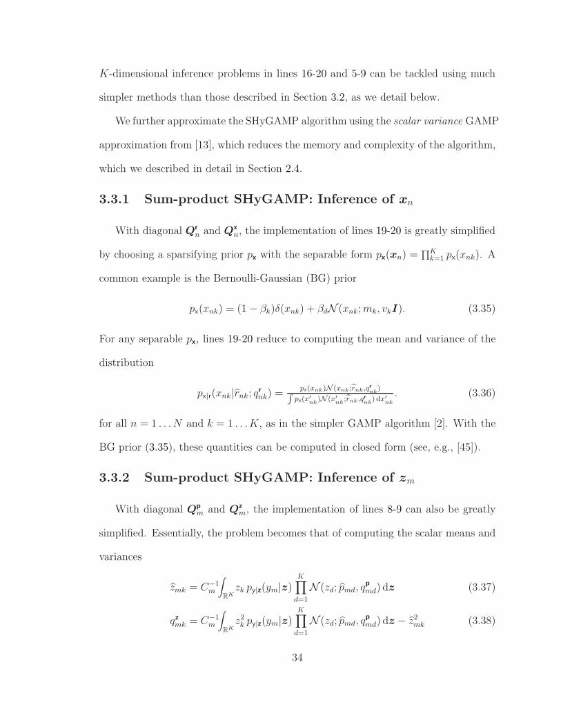
3.3.1 Sum-product SHyGAMP: Inference of xn . . . . . . . . . . 343.3.2 Sum-product SHyGAMP: Inference of zm . . . . . . . . . . 34

3.3.3 Min-sum SHyGAMP: Inference of xn . . . . . . . . . . . . . 403.3.4 Min-sum SHyGAMP: Inference of zm . . . . . . . . . . . . 41

3.3.5 SHyGAMP summary . . . . . . . . . . . . . . . . . . . . . . 433.4 Online Parameter Tuning . . . . . . . . . . . . . . . . . . . . . . . 44

3.4.1 Parameter selection for Sum-product SHyGAMP . . . . . . 443.4.2 Parameter selection for Min-sum SHyGAMP . . . . . . . . 44

3.5 Numerical Experiments . . . . . . . . . . . . . . . . . . . . . . . . 473.5.1 Synthetic data in the M ≪ N regime . . . . . . . . . . . . . 48

3.5.2 Example of SURE tuning . . . . . . . . . . . . . . . . . . . 503.5.3 Micro-array gene expression . . . . . . . . . . . . . . . . . . 54

3.5.4 Text classification with the RCV1 dataset . . . . . . . . . . 57

3.5.5 MNIST handwritten digit recognition . . . . . . . . . . . . 593.6 Conclusion . . . . . . . . . . . . . . . . . . . . . . . . . . . . . . . 59

4. Sketched Clustering via Approximate Message Passing . . . . . . . . . . 62

4.1 Introduction . . . . . . . . . . . . . . . . . . . . . . . . . . . . . . 624.1.1 Sketched Clustering . . . . . . . . . . . . . . . . . . . . . . 63

4.1.2 Contributions . . . . . . . . . . . . . . . . . . . . . . . . . . 644.2 Compressive Learning via AMP . . . . . . . . . . . . . . . . . . . . 65

4.2.1 High-Dimensional Inference Framework . . . . . . . . . . . 654.2.2 Approximate Message Passing . . . . . . . . . . . . . . . . . 67

4.2.3 From SHyGAMP to CL-AMP . . . . . . . . . . . . . . . . . 684.2.4 Initialization . . . . . . . . . . . . . . . . . . . . . . . . . . 76

4.2.5 Hyperparameter Tuning . . . . . . . . . . . . . . . . . . . . 774.2.6 Algorithm Summary . . . . . . . . . . . . . . . . . . . . . . 79

ix

4.2.7 Frequency Generation . . . . . . . . . . . . . . . . . . . . . 794.3 Numerical Experiments . . . . . . . . . . . . . . . . . . . . . . . . 80

4.3.1 Experiments with Synthetic Data . . . . . . . . . . . . . . . 814.3.2 Spectral Clustering of MNIST . . . . . . . . . . . . . . . . . 91

4.3.3 Frequency Estimation . . . . . . . . . . . . . . . . . . . . . 944.4 Conclusion . . . . . . . . . . . . . . . . . . . . . . . . . . . . . . . 98

5. Adaptive Detection from Quantized Measurements . . . . . . . . . . . . 103

5.1 Introduction and Motivation . . . . . . . . . . . . . . . . . . . . . . 1035.1.1 Problem Statement . . . . . . . . . . . . . . . . . . . . . . . 104

5.1.2 Unquantized Detectors . . . . . . . . . . . . . . . . . . . . . 105

5.2 Numerical Study of Unquantized Detectors with Quantized Mea-surements . . . . . . . . . . . . . . . . . . . . . . . . . . . . . . . . 106

5.2.1 Summary . . . . . . . . . . . . . . . . . . . . . . . . . . . . 1105.3 Detection Performance with Dither and Companding . . . . . . . . 111

5.3.1 Detection Performance with a Dithered Quantizer . . . . . . 1125.3.2 Detection Performance with Non-uniform Quantization . . . 114

5.4 The GLRT with the Quantized Model . . . . . . . . . . . . . . . . 1155.4.1 The GLRT in the 1-bit Case . . . . . . . . . . . . . . . . . 117

5.4.2 Multi-bit Case . . . . . . . . . . . . . . . . . . . . . . . . . 1225.4.3 Summary of the GLRT . . . . . . . . . . . . . . . . . . . . 126

5.4.4 Numerical Results . . . . . . . . . . . . . . . . . . . . . . . 1265.4.5 Summary . . . . . . . . . . . . . . . . . . . . . . . . . . . . 129

5.5 Pre-processing Techniques . . . . . . . . . . . . . . . . . . . . . . . 1295.5.1 Beamforming . . . . . . . . . . . . . . . . . . . . . . . . . . 130

5.5.2 Pre-Whitening . . . . . . . . . . . . . . . . . . . . . . . . . 131

5.6 Conclusion . . . . . . . . . . . . . . . . . . . . . . . . . . . . . . . 136

6. Conclusion . . . . . . . . . . . . . . . . . . . . . . . . . . . . . . . . . . . 139

Bibliography . . . . . . . . . . . . . . . . . . . . . . . . . . . . . . . . . . . . 141

x

List of Figures

Figure Page

2.1 Factor graph . . . . . . . . . . . . . . . . . . . . . . . . . . . . . . . . 14

3.1 Full and reduced factor graphs . . . . . . . . . . . . . . . . . . . . . . 26

3.2 Estimator MSE vs Variance . . . . . . . . . . . . . . . . . . . . . . . 41

3.3 Estimator Runtime vs K . . . . . . . . . . . . . . . . . . . . . . . . . 42

3.4 Test error rate and runtime vs M . . . . . . . . . . . . . . . . . . . . 51

3.5 Test error rate and runtime vs S . . . . . . . . . . . . . . . . . . . . . 52

3.6 Test error rate and runtime vs N . . . . . . . . . . . . . . . . . . . . 53

3.7 Test error rate vs λ . . . . . . . . . . . . . . . . . . . . . . . . . . . . 54

3.8 Test-error rate versus runtime for the RCV1 dataset. . . . . . . . . . 58

3.9 Test error rate vs M for the MNIST dataset . . . . . . . . . . . . . . 60

4.1 SSE vs. sketch length M . . . . . . . . . . . . . . . . . . . . . . . . . 83

4.2 Classification error rate vs. sketch length M . . . . . . . . . . . . . . 84

4.3 Runtime (including sketching) vs. sketch length M . . . . . . . . . . 85

4.4 SSE vs. number of clusters K . . . . . . . . . . . . . . . . . . . . . . 86

4.5 Classification Error Rate vs. number of clusters K . . . . . . . . . . . 87

xi

4.6 Runtime (including sketching) vs. number of clusters K . . . . . . . . 88

4.7 SSE/N vs. dimension N . . . . . . . . . . . . . . . . . . . . . . . . . 89

4.8 Classification Error Rate vs. dimension N . . . . . . . . . . . . . . . 90

4.9 Runtime (including sketching) vs. dimension N . . . . . . . . . . . . 91

4.10 Clustering performance vs. training size T . . . . . . . . . . . . . . . 92

4.11 Runtime vs. training size T . . . . . . . . . . . . . . . . . . . . . . . 93

4.12 SSE vs. M for the T = 70 000-sample spectral MNIST dataset . . . . 95

4.13 CER vs. M for the T = 70 000-sample spectral MNIST dataset . . . . 96

4.14 Runtime vs. M on the 70k-sample MNIST dataset . . . . . . . . . . . 97

4.15 SSE vs. M for the T = 300 000-sample spectral MNIST dataset . . . 98

4.16 CER vs. M for the T = 300 000-sample spectral MNIST dataset . . . 99

4.17 Runtime vs. M on the 300k-sample MNIST dataset . . . . . . . . . . 100

4.18 Frequency estimation with random time samples . . . . . . . . . . . . 101

4.19 Frequency estimation with uniform time samples . . . . . . . . . . . . 102

5.1 Detection probability vs noise power . . . . . . . . . . . . . . . . . . 108

5.2 SNR gain vs B . . . . . . . . . . . . . . . . . . . . . . . . . . . . . . 110

5.3 Detection probability vs interference power . . . . . . . . . . . . . . . 111

5.4 ISR gain vs B . . . . . . . . . . . . . . . . . . . . . . . . . . . . . . . 112

5.5 PD vs σ2i /ns for various dither signals. . . . . . . . . . . . . . . . . . 113

5.6 PD vs σ2i /ns for various dither signals. . . . . . . . . . . . . . . . . . 114

5.7 PD vs σ2i /ns with companding. . . . . . . . . . . . . . . . . . . . . . . 116

xii

5.8 PD vs σ2i /ns with PCA. . . . . . . . . . . . . . . . . . . . . . . . . . 127

5.9 ROC curves of various detectors for different B . . . . . . . . . . . . 128

5.10 PD vs σ2i /ns with different beamforming techniques. . . . . . . . . . . 132

5.11 PD vs σ2i /ns with iterative whitening technique. . . . . . . . . . . . . 135

5.12 PD vs σ2i /ns with iterative whitening technique, unit-modulus case . . 136

5.13 PD vs σ2i /ns with iterative whitening technique, discrete-phase case . 137

xiii

List of Tables

Table Page

2.1 The HyGAMP Algorithm . . . . . . . . . . . . . . . . . . . . . . . . 16

3.1 A summary of GAMP for SMLR . . . . . . . . . . . . . . . . . . . . 33

3.2 A summary of SGAMP for SMLR . . . . . . . . . . . . . . . . . . . . 43

3.3 High-level comparison of SHyGAMP and HyGAMP. . . . . . . . . . . 43

3.4 Configurations of the synthetic-data experiments. . . . . . . . . . . . 49

3.5 Experimental results for the Sun dataset. . . . . . . . . . . . . . . . . 56

3.6 Experimental results for the Bhattacharjee dataset . . . . . . . . . . 57

4.1 SPA-SHyGAMP for Sketched Clustering . . . . . . . . . . . . . . . . 69

4.2 CL-AMP with parameter tuning and multiple initializations . . . . . 80

xiv

Chapter 1: Introduction

In this dissertation we consider a wide variety of inference problems that involve

the generalized linear model (GLM). We begin with several motivating examples that

stem from the prominence of “Big Data”, where the datasets may be very large and

the challenge is to efficiently process the data in a manner that makes useful insights.

Our first example is the feature selection problem in the field of genomics. In

this problem one is given gene-expression data from several patients, each patient

with a specific (known) disease, and tasked with determining which genes predict the

presence of each disease. The challenging aspect of this problem is that the number

of features, which in this problem are the potentially predictive genes, is very large

(typically tens of thousands of genes), and, due to the cost of obtaining the data,

is much larger than the number of gene-expression samples per disease (typically

dozens).

Our second application is the classification problem; here we consider document

classification as an example. In this problem the goal is to use the relative frequency

of the various keywords to predict the subject area of future documents. In order to

design a prediction rule, one is given a training dataset where each sample corresponds

to a document in a specific, known, subject area, and the features of the sample are

the relative frequency of various keywords. Two aspects of this problem that make it

1

challenging are: 1) the number of different subject areas may be large (more than 10),

and 2) designing a decision rule from the dataset may be computationally challenging

due to its sheer size. For example, a dataset in this domain may contain hundreds of

thousands of samples and each sample contains tens of thousands of features.

Another application is the clustering problem, which is similar to the classification

problem, except here the datasets are “unlabeled” and the goal is to partition the

samples into their appropriate classes. For example, there may be a large dataset

containing images of handwritten digits, where the class corresponds to the digit

(0-9), but prior to designing a classifier with this dataset the samples must first be

labeled. Labeling by hand is not a feasible option due to the large quantity of samples,

and more importantly, in many applications a human may not be able to correctly

determine the class. Therefore, an algorithm that can accurately partition the dataset

into clusters is desired.

A final application is the detection problem in array processing. Here, one may

sample incoming radio signals across both space (using multiple antennas) and time

(using multiple temporal snapshots) with the goal of determining the presence or

absence of a specific signal while in the presence of corrupting noise and interference.

Two practical uses for this problem are in radar and in wireless communications. In

radar one emits a known signal and makes estimates of the scene based on properties of

the reflected signal, while in communications one user emits a known synchronization

signal to another user in order for a connection to be fully established. In these

examples, if many antennas (dozens) and time snapshots (thousands) are used, the

entire block of data may be quite large and computationally challenging to process.

2

In addition, practical effects such as quantization, which distort the measured signal,

may have a large effect on performance and should be considered in the design.

There are many approaches to tackling the aforementioned problems, some of

which involve inference with the GLM. In the sequel, we introduce the GLM and

commonly applied maximum likelihood (ML) and maximum a posteriori (MAP) in-

ference framework.

1.1 Introduction to Generalized Linear Models

1.1.1 The Standard Linear Model

Prior to describing the GLM, we first present the standard linear model, given by

y = Ax + w, (1.1)

where y ∈ RM is a vector of measurements, A ∈ RM×N is a known linear operator,

and w is independent and identically distributed (iid) Gaussian noise. Our objective

is to infer x. There are various approaches to doing so. Perhaps the most funda-

mental is the maximum likelihood (ML) estimation framework, which makes no prior

assumptions on x and solves

xML = arg maxx

log p(y|x) (1.2)

= arg minx‖y −Ax‖22 (1.3)

= A+y, (1.4)

where A+ is the pseudoinverse of A and (1.3) follows from (1.2) due to the iid

Gaussian assumption on w.

The solution given by (1.4) is not always desirable. For example, if M < N , (1.4)

is one of infinitely many solutions to Problem (1.2), or it may not be near the true

3

x. However, this problem may be circumvented by maximum a posteriori (MAP)

estimation, where one specifies a prior p(x) that imparts a desired structure on the

estimate x. For example, in Compressed Sensing (CS), one hypothesizes that x is

sparse, i.e., it contains mostly zeros, say S < N non-zero elements. If S < M , it

may be possible to find an accurate estimate x. Therefore, one applies the Laplacian

prior p(x) ∝ exp(−λ‖x‖1), which promotes learning a sparse x. This results in the

LASSO problem, given by

xLASSO = arg minx

{‖y −Ax‖22 + λ‖x‖1

}, (1.5)

where λ controls the strength of this regularization; the larger λ, the more sparse

xLASSO will be.

1.1.2 The Generalized Linear Model

In the standard linear model, the measurements y are Gaussian-noise corrupted

versions of the “noiseless” measurements z , Ax. The GLM instead models p(y|z)

as an arbitrary likelihood that need not correspond to additive white Gaussian noise.

The objective remains to learn x, possibly under prior assumptions, while using the

arbitrary likelihood p(y|z).

A popular example of the GLM is logistic regression. Logistic regression is one

approach to binary linear classification and feature selection. In binary linear clas-

sification, one is given M feature vectors with corresponding binary class labels{am ∈ RN , ym ∈ {−1, 1}

}M

m=1with the goal of designing a weight vector x that

accurately classifies a test feature vector a0, where classification is performed via

y0 = sgn aT0 x. For example, if one considers the genomics problem described in the

4

first part of this chapter, ym may indicate one of two possible disease types, while

elements in am represent the expression level of individual genes.

In logistic regression, we model

p(ym|zm = aTmx) =

1

1 + exp(−ymzm), (1.6)

which takes values between 0 and 1 and models that probability that am belongs to

class ym with the decision boundary defined by x.

The ML approach to logistic regression is to solve

xML = arg maxx

log p(y|z = Ax) (1.7)

= arg maxx

M∑

m=1

log1

1 + exp(−ymaTmx)

, (1.8)

where aTm form the rows of A. However, similar to the linear case, issues may arise

with xML. For example, if the data is linearly separable, then xML will be infinite

valued.

MAP estimation offers a resolution. For example, a Gaussian prior on x (which

is equivalent to quadratic regularization ‖x‖22) will prevent the estimate from being

infinite valued, even in the linearly separable case. Or, similar to the CS problem, if

we can correctly hypothesize that only S < M features (elements of am) are useful

for classification, accurate classification may be achieved by learning an S-sparse x,

which may be achieved by incorporating a λ‖x‖1 regularization, in which case we

have

xMAP = arg maxx

{log p(y|z = Ax)− λ‖x‖1

}. (1.9)

Referring back to the genomics problem, feature selection can be performed by looking

at the support of sparse xMAP.

5

GLMs with Additional Structure

So far, we have considered problems where ym depends only on a scalar zm. How-

ever, there exist GLMs with additional structure. One example is where X ∈ RN×K

and ym depends on zm , XTam ∈ RK . An example is multinomial logistic regres-

sion, which is the multi-class extension of logistic regression. In multinomial logistic

regression we still have am ∈ RN , but now ym ∈ {1, ..., K}, indicating to which of K

classes am belongs. The probability that am belongs to class ym ∈ {1, ..., K}, given

decision boundaries parameterized by X, is now modeled by the “softmax” equation

p(ym|zm = XTam) =exp

([zm]ym

)

∑Kk=1 exp

([zm]k

) (1.10)

and classification of a0 is performed via y0 = arg maxk[z0]k. Problems involving

inference in these types of GLMs are a primary focus of this dissertation.

1.1.3 The Generalized Bilinear Model

The generalized bilinear model is similar to the GLM, except that now A and

X must both be estimated. One example is binary principal components analysis

(PCA) (which is discussed more in Chapter 5), where we have

Y = sgn(AX + W ) (1.11)

and wish to infer A and X, possibly under a rank constraint. Assuming elements in

W are iid Gaussian with variance σ2w, then

p(Y |A, X) =N∏

n=1

M∏

m=1

Φ(

ynmznm

σw

), (1.12)

where Φ(·) is the standard normal CDF and znm = [AX ]nm. Then, one could solve

{A, X

}= arg max

A,Xlog p(Y |A, X) s.t. rank(AX) ≤ R. (1.13)

6

1.1.4 Summary

So far, we have introduced linear and generalized linear models, with various

examples. We have also introduced the ML and MAP inference frameworks, where

one first has to specify p(y|z). Then, one may specify a regularization λg(x), which

corresponds to the prior p(x) ∝ exp(λg(x)

). Combining these, one can solve

xMAP = arg maxx

{log p(y|z = Ax) + λg(x)

}. (1.14)

There are advantages and disadvantages of this approach. Problem (1.14) is inter-

pretable and convex for many choices of p(y|z) and g(x). However, iterative methods

to solve Problem (1.14) may require many iterations to converge, leading to a large

computational cost of this approach. This high computational cost is exacerbated

when A is large because each iteration is more costly. Additionally, the complexity is

further increased when λ and hyperparameters associated with p(y|z) must be tuned,

where cross-validation (CV) is the standard approach and involves solving Problem

(1.14) with multiple subsets of A and multiple hypothesized values of λ (and any

other hyperparameter). Moreover, Problem (1.14) is just one type of estimation.

There are others, such as minimum mean square error (MMSE) that may be more

desirable for some problems, but are in general not as numerically tractable as MAP

estimation. In the next section we introduce a class of inference algorithms based on

Approximate Message Passing that address some of these issues.

1.2 Introduction to Approximate Message Passing

In this section we introduce Approximate Message Passing (AMP), which are a

class of algorithms well suited to inference in the linear and generalized linear models.

7

To address the issues mentioned in Section 1.1.4, approximately a decade ago,

the original AMP algorithm of Donoho, Maleki, and Montanari [1] was created for

inference with the standard linear model in (1.1). AMP assumes elements in A are

iid sub-Gaussian, and requires a separable prior on x, i.e., px(x) =∏N

n=1 px(xn). The

AMP algorithm then uses various approximations based on the central limit theorem

and Taylor series to approximate MAP or MMSE inference by approximating the sum-

product (SPA) or min-sum (MSA) loopy belief propagation algorithms, respectively,

on the factor graph associated with (1.1) and px(x). AMP was originally applied to

the LASSO problem in (1.5) by setting log px(xn) = −λ|xn| + const., where it was

demonstrated to converge in substantially fewer iterations than existing state-of-that-

art algorithms.

However, AMP is restrictive due to its AWGN-only assumption. Subsequently,

AMP was extended by Rangan [2] to generalized linear models, yielding the Gen-

eralized AMP (GAMP) algorithm. GAMP still requires separable px(x), and also

requires py|z(y|z) =∏M

m=1 py|z(ym|zm), which combine to form the posterior

px|y(x|y) ∝M∏

m=1

py|z(ym|zm)N∏

n=1

px(xn). (1.15)

AMP and GAMP have several advantages over conventional techniques for infer-

ence in the standard and generalized linear models. First, both AMP and GAMP

give accurate approximations of the SPA and MSA under large i.i.d. sub-Gaussian A,

while maintaining a computational complexity of only O(MN). Through numerical

simulations, both AMP and GAMP have been demonstrated to be superior to existing

state-of-the-art inference techniques for a wide variety of applications. Furthermore,

both can be rigorously analyzed via the state-evolution framework, which proves that

they compute MMSE optimal estimates of x in certain regimes [3]. Finally, the

8

GAMP algorithm can be readily combined with the expectation-maximization (EM)

algorithm to tune hyperparameters associated with py|z and px online, avoiding the

need to perform expensive cross-validation [4].

A limitation of AMP [1] and GAMP [2] is that they treat only problems with i.i.d.

estimand x and separable, scalar, likelihood p(y|z) =∏M

m=1 p(ym|zm). Thus, Hybrid

GAMP (HyGAMP) [5] was developed to tackle problems with a structured prior

and/or likelihood. Specifically, HyGAMP allows structure on py|z first mentioned in

Section 1.1.2, and allows structure on rows of X, provided by the prior px(xn) i.e.,

HyGAMP assumes the probabilistic model

pX|y(X|y) =M∏

m=1

py|z(ym|zm)N∏

n=1

px(xn), (1.16)

where py|z(ym|zm) 6= ∏Kk=1 py|z(ym|zmk), and xT

n is the nth row of X (so, for example, a

prior could be constructed to encourage row-sparsity in X). The HyGAMP algorithm

will be described in more detail in Chapter 2.

Finally, AMP has also been extended to generalized bilinear inference, for example

in the BiGAMP [6] and LowRAMP [7,8] algorithms, both of which assume the model

pX|Y(X|Y ) ∝

M∏

m=1

K∏

k=1

py|z(ymk|zmk)

N∏

n=1

K∏

k=1

px(xnk)

M∏

m=1

N∏

n=1

pa(amn)

, (1.17)

but differ in their specific approximation to the sum-product algorithm.

1.3 Outline and Contributions

An outline of this dissertation and our research contributions are summarized

here.

9

1.3.1 The HyGAMP Algorithm

First, in Chapter 2 we present the HyGAMP algorithm [5], which is an exten-

sion of the GAMP algorithm to the structured p(ym|zm) presented in Section 1.1.2.

Similar to GAMP, the HyGAMP algorithm comes in two flavors: SPA-HyGAMP

and MSA-HyGAMP, which approximate MMSE and MAP estimation, respectively.

Then, we explain the “simplified” version of the HyGAMP algorithm, first presented

in [9], (SHyGAMP), which drastically reduces the computational complexity of its

implementation and allows this approach to be computationally competitive with

existing state-of-the-art approaches for various applications.

1.3.2 Sparse Multinomial Logistic Regression

In Chapter 3 we apply the SPA and MSA HyGAMP algorithms from Chapter 2

to the sparse multinomial logistic regression (SMLR) problem [10]. In this prob-

lem we are given training data consisting of feature-vector, label pairs {am, ym}Mm=1,

am ∈ RN , ym ∈ {1, ..., K} with the goal of designing a weight matrix X ∈ RN×K

that accurately predicts the class label y0 on the unlabeled feature vector a0, via

y0 = arg maxk[XTa0]k. The multinomial logistic regression approach to this problem

models the probability that am belongs to class ym via

p(ym|zm) =exp

([zm]ym

)

∑Kk=1 exp

([zm]k

) , (1.18)

where zm = XTam. HyGAMP can be applied to this problem by using (1.18)

in (1.15). We focus on the regime where M < N and therefore use a sparsity-

promoting prior p(X). We note that while the MSA-HyGAMP algorithm agrees

with the standard MAP estimation technique [10] for this problem, we show that

the SPA-HyGAMP approach can be interpreted as the test-error-rate-minimizing

10

approach to designing the weight matrix X. Then, we extend both the SPA and

MSA HyGAMP algorithms to their SHyGAMP counterparts, after which we show

through extensive numerical experiments that our approach surpasses existing state-

of-the-art approaches to the SMLR problem in both accuracy and computational

complexity.

1.3.3 Sketched Clustering

In Chapter 4 we apply the SPA-SHyGAMP algorithm from Chapter 2 to the

sketched clustering problem [11,12]. The sketched clustering problem is a variation of

the traditional clustering problem, where one is given a dataset D ∈ RN×T comprising

of T feature-vectors of dimension N , and wants to find K centroids X = [x1, ..., xK ] ∈

RN×K that minimize the sum of squared errors (SSE), where

SSE(X, D) =1

T

T∑

t=1

mink‖dt − xk‖22. (1.19)

The sketched clustering approach to this problem first “sketches” the data matrix

D into a relatively low dimensional vector y via a non-linear transformation. Then,

a sketched clustering recovery algorithm attempts to extract X from y instead of D.

In Chapter 4, with our particular choice of sketching function, we show how we

are able to apply the SPA-SHyGAMP algorithm to this problem. We then show

through numerical experiments that our approach, in some regimes, has better ac-

curacy, computational complexity, and memory complexity than k-means, and has

better time and sample complexity than the only other known sketched clustering

algorithm, CL-OMPR [12].

11

1.3.4 Adaptive Detection from Quantized Measurements

Finally, in Chapter 5 we shift gears and investigate adaptive detection using quan-

tized measurements. First, we study the effects of using unquantized detection tech-

niques but with quantized measurements. We observe that there is not a significant

loss to using quantized measurements, as long as the interference power is small. How-

ever, when the interference power is large, the lack of dynamic range in the quantizer

eliminates any chance for reliable detection. We then investigate and develop several

techniques to improve detection performance in the high-interference regime. First,

we consider two basic techniques that are commonly used in conjunction with quan-

tized measurements: dithering and companding. Then, we develop and apply the

generalized likelihood ratio test (GLRT) to this problem using the appropriate quan-

tization and noise model, which results in a generalized linear model. We observe

this approach does not offer significant improvement, so we conclude with a vari-

ety of proposed techniques that are based upon applying an interference-reduction

transformation to the data in the analog domain prior to quantization.

12

Chapter 2: The Hybrid-GAMP Algorithm

In this Chapter, we present a special case1 of the hybrid generalized approximate

message passing (HyGAMP) algorithm [5] that will later be used to tackle the multi-

nomial logistic regression problem in Chapter 3 and the sketched clustering problem

in Chapter 4. The HyGAMP algorithm is an extension of the AMP and GAMP

algorithms originally introduced in Section 1.2.

2.1 Model

HyGAMP assumes the probabilistic model

pX|y(X|y) ∝M∏

m=1

py|z(ym|zm)N∏

n=1

px(xn), (2.1)

where xTn is the nth row of X ∈ RN×K and zT

m is the mth row of Z = AX, where

A ∈ RM×N . Under (2.1), the HyGAMP algorithm approximates either

XMMSE , E{X|y} (2.2)

or

XMAP , arg maxX

log pX|y(X|y) (2.3)

1In particular, the “hybrid” in HyGAMP refers to combining approximate message passing withexact message passing. However, we do not use that feature of HyGAMP and therefore do notpresent it for simplicity. The version of HyGAMP that we present is a simple generalization of theGAMP algorithm (i.e., GAMP and HyGAMP coincide when K = 1). The “hybrid” modifier istherefore unnecessary, but we retain it to remain consistent with previously published works.

13

pym|zm

xn

ym

pxn

Figure 2.1: Factor graph representations of (2.1), with white/gray circles denotingunobserved/observed random variables, and gray rectangles denoting pdf “factors”.

by approximating the sum-product (SPA) or min-sum (MSA) loopy belief propagation

algorithms, respectively, on the factor graph associated with (2.1), which is shown

in Figure 2.1. Throughout this document we may use the terms SPA-HyGAMP and

MMSE-HyGAMP interchangeably, likewise with MSA/MAP HyGAMP.

2.2 The HyGAMP Algorithm

The HyGAMP algorithm is presented in Table 2.1. It requires matrix A and

measurement vector y, we well as the distributions px|r and pz|y,p, which are given in

(2.4) and (2.5) and depend on px(xn) and py|z(ym|zm), respectively. It also requires

initialization xn(0) and Qxn(0); we note the specific choice of initialization depends

on the application and more details will be given at the appropriate time.

Observe that HyGAMP breaks the N ×K dimensional inference problem into a

sequence of K-dimensional inference problems, which are shown in Lines 5-9 and 16-20

of Table 2.1. Not surprisingly, in the MAP case, the K-dimensional inference problems

involve MAP estimation, while in the MMSE case the inference problems require

14

MMSE estimation. They involve the following approximate posterior distributions

on xn and zm, respectively:

px|r(xn|rn; Qrn) =

px(xn)N (xn; rn, Qrn)

∫px(x′

n)N (x′n; rn, Q

rn) dx′

n

(2.4)

and

pz|y,p(zm|ym, pm; Qpm) =

py|z(ym|zm)N (zm; pm, Qpm)

∫py|z(ym|z′

m)N (z′m; pm, Qp

m) dz′m

. (2.5)

These distributions depend on the choice of px(xn) and py|z(ym|zm). As we will see in

future chapters, these low-dimensional inference problems may be non-trivial to solve

for certain choices of px(xn) and py|z(ym|zm).

In the large system limit with iid Gaussian A, rn can be interpreted as a Gaussian

noise corrupted version of the true xn with noise distribution N (0, Qrn), and similarly

pm as a Gaussian noise corrupted version of the true zm with noise distribution

N (0, Qpm). Note that in many applications, A is not iid Gaussian, but treating it as

such appears to work sufficiently well.

2.3 Simplified HyGAMP

Excluding the inference steps in lines 5-9 and 16-20 of Table 2.1, the computational

complexity of HyGAMP is O(MNK2 + (M + N)K3

), where the “MNK2” term is

from line 2, and the “(M + N)K3” term is from lines 11 and 13, where it requires

computing O(M +N) K×K matrix inversions at every iteration. The computational

complexity of the inference steps are excluded because they depend on py|z and px.

However, they may be complicated due to both the form of py|z and px and full

covariance matrices Qxn, Qr

n, etc.

15

Require: Mode ∈ {SPA, MSA}, matrix A, vector y, pdfs px|r and pz|y,p from (2.4)-(2.5),initializations xn(0), Qx

n(0).Ensure: t←0; sm(0)←0.1: repeat

2: ∀m : Qpm(t)← ∑N

n=1 A2mnQ

xn(t)

3: ∀m : pm(t)← ∑Nn=1 Amnxn(t)−Qp

m(t)sm(t)4: if MSA then {for m = 1 . . .M}5: zm(t)← arg maxz log pz|y,p

(zm

∣∣∣ym, pm(t); Qpm(t)

)

6: Qzm(t)←

[− ∂2

∂z2 log pz|y,p

(zm(t)

∣∣∣ym, pm(t); Qpm(t)

)]−1

7: else if SPA then {for m = 1 . . .M}8: zm(t)← E

{zm

∣∣∣ ym, pm = pm(t); Qpm(t)

}

9: Qzm(t)← Cov

{zm

∣∣∣ ym, pm = pm(t); Qpm(t)

}

10: end if

11: ∀m : Qsm(t)← [Qp

m(t)]−1 − [Qpm(t)]−1Qz

m(t)[Qpm(t)]−1

12: ∀m : sm(t + 1)← [Qpm(t)]−1

(zm(t)− pm(t)

)

13: ∀n : Qrn(t)←

[∑Mm=1 A2

mnQsm(t)

]−1

14: ∀n : rn(t)← xn(t) + Qrn(t)

∑Mm=1 Amnsm(t + 1)

15: if MSA then {for n = 1 . . . N}16: xn(t + 1)← arg maxx log px|r

(xn

∣∣∣rn(t); Qrn(t)

)

17: Qxn(t + 1)←

[− ∂2

∂x2 log px|r

(xn(t + 1)

∣∣∣rn(t); Qrn(t)

)]−1

18: else if SPA then {for n = 1 . . .N}19: xn(t + 1)← E

{xn

∣∣∣ rn = rn(t); Qrn(t)

}

20: Qxn(t + 1)← Cov

{xn

∣∣∣ rn = rn(t); Qrn(t)

}

21: end if

22: t← t + 123: until Terminated

Table 2.1: The HyGAMP Algorithm. For clarity, note that all matrices Qxn, Qz

m, etcare K ×K, and vectors xn, zm, pm, etc are K × 1.

For our work in sparse multinomial logistic regression and sketched clustering, we

proposed a simplified HyGAMP (SHyGAMP) in order to be computationally compet-

itive with existing state-of-the-art algorithms for those applications. In SHyGAMP,

16

we simply force all covariance matrices in Table 2.1, e.g., Qxn, Qp

m, etc, to be diag-

onal, e.g., Qxn = diag{qx

n1, ..., qxnK}. In many applications we have found when we

compared SHyGAMP to HyGAMP that SHyGAMP had negligible loss in accuracy,

while having a drastic decrease in computational complexity. In particular, the com-

putational complexity of SHyGAMP (excluding the inference steps) is O(MNK).

Furthermore, for many choices of py|z and px, using diagonal covariance matrices Qxn,

Qrn, etc decreases the computational complexity of the inference steps.

2.4 Scalar-variance Approximation

We further approximate the SHyGAMP algorithm using the scalar variance GAMP

approximation from [13], which reduces the memory and complexity of the algorithm.

The scalar variance approximation first approximates the variances {qxnk} by a value

invariant to both n and k, i.e.,

qx ,1

NK

N∑

n=1

K∑

k=1

qxnk. (2.6)

Then, in line 2 in Table 2.1, we use the approximation

qpmk ≈

N∑

n=1

A2mnq

x(a)≈ ‖A‖

2F

Mqx , qp. (2.7)

The approximation (a), after precomputing ‖A‖2F , reduces the complexity of line 2

from O(NK) to O(1). We next define

qs ,1

MK

M∑

m=1

K∑

k=1

qsmk (2.8)

and in line 13 we use the approximation

qrnk ≈

(M∑

m=1

A2mnq

s

)−1

≈ N

qs‖A‖2F, qr. (2.9)

17

The complexity of line 13 then simplifies from O(MK) to O(1). For clarity, we note

that after applying the scalar variance approximation, we have Qxn = qxIK ∀n, and

similar for Qrn, Qp

m and Qzm.

2.5 Conclusion

The HyGAMP algorithm is an extension of the GAMP algorithm to inference

problems with additional structure on py|z, notably the case where py|z(ym|zm) 6=∏K

k=1 py|z(ym|zmk). The HyGAMP algorithm can be applied to many inference prob-

lems by appropriately selecting px and py|z. However, as we will see in future chapters,

for many choices of px and py|z, the inference problems in Lines 5-9 and 16-20 of Ta-

ble 2.1 are non-trivial to compute. Moreover, the HyGAMP algorithm is complicated

by the full covariance matrices Qx, etc, and so for practical considerations a simpli-

fied version, SHyGAMP, is proposed. In Chapters 3 and 4, we apply the SHyGAMP

algorithm to the problems or sparse multinomial logistic regression and sketched clus-

tering, respectively.

18

Chapter 3: Sparse Multinomial Logistic Regression via

Approximate Message Passing

3.1 Introduction

In this chapter2, we consider the problems of multiclass (or polytomous) linear

classification and feature selection. In both problems, one is given training data of

the form {(ym, am)}Mm=1, where am ∈ RN is a vector of features and ym ∈ {1, . . . , K}

is the corresponding K-ary class label. In multiclass classification, the goal is to infer

the unknown label y0 associated with a newly observed feature vector a0. In the

linear approach to this problem, the training data are used to design a weight matrix

X ∈ RN×K that generates a vector of “scores” z0 , XTa0 ∈ R

K , the largest of which

can be used to predict the unknown label, i.e.,

y0 = arg maxk

[z0]k. (3.1)

In feature selection, the goal is to determine which subset of the N features a0 is

needed to accurately predict the label y0.

2Work presented in this chapter is largely excerpted from a journal publication co-authored withPhilip Schniter, titled “Sparse Multinomial Logistic Regression via Approximate Message Passing”[9]. We note that a preliminary version of this work was published in the Master’s Thesis authoredby Evan Byrne [14]. It is included here as well to include changes made during the peer-reviewprocess, and because it forms part of a larger story when combined with the other chapters of thisdissertation.

19

We are particularly interested in the setting where the number of features, N , is

large and greatly exceeds the number of training examples, M . Such problems arise

in a number of important applications, such as micro-array gene expression [15, 16],

multi-voxel pattern analysis (MVPA) [17, 18], text mining [19, 20], and analysis of

marketing data [21].

In the N ≫ M case, accurate linear classification and feature selection may be

possible if the labels are influenced by a sufficiently small number, S, of the total

N features. For example, in binary linear classification, performance guarantees are

possible with only M = O(S log N/S) training examples when am is i.i.d. Gaussian

[22].

Note that, when S ≪ N , accurate linear classification can be accomplished using

a sparse weight matrix X , i.e., a matrix where all but a few rows are zero-valued.

3.1.1 Multinomial logistic regression

For multiclass linear classification and feature selection, we focus on the approach

known as multinomial logistic regression (MLR) [23], which can be described using

a generative probabilistic model. Here, the label vector y , [y1, . . . , yM ]T is modeled

as a realization of a random3 vector y , [y1, . . . , yM ]T, the “true” weight matrix X is

modeled as a realization of a random matrix X, and the features A , [a1, . . . , aM ]T

are treated as deterministic. Moreover, the labels ym are modeled as conditionally

independent given the scores zm , XTam, i.e.,

Pr{y = y |X = X; A} =M∏

m=1

py|z(ym|XTam), (3.2)

3For clarity, we typeset random quantities in sans-serif font and deterministic quantities in seriffont.

20

and distributed according to the multinomial logistic (or soft-max) pmf:

py|z(ym|zm) =exp([zm]ym)

∑Kk=1 exp([zm]k)

, ym ∈ {1, . . . , K}. (3.3)

The rows xTn of the weight matrix X are then modeled as i.i.d.,

pX(X) =N∏

n=1

px(xn), (3.4)

where px may be chosen to promote sparsity.

3.1.2 Existing methods

Several sparsity-promoting MLR algorithms have been proposed (e.g., [10,24–28]),

differing in their choice of px and methodology of estimating X. For example, [10,25,

26] use the i.i.d. Laplacian prior

px(xn; λ) =K∏

k=1

λ

2exp(−λ|xnk|), (3.5)

with λ tuned via cross-validation. To circumvent this tuning problem, [27] employs

the Laplacian scale mixture

px(xn) =K∏

k=1

∫ [λ

2exp(−λ|xnk|)

]p(λ) dλ, (3.6)

with Jeffrey’s non-informative hyperprior p(λ) ∝ 1λ1λ≥0. The relevance vector ma-

chine (RVM) approach [24] uses the Gaussian scale mixture

px(xn) =K∏

k=1

∫N (xnk; 0, ν)p(ν) dν, (3.7)

with inverse-gamma p(ν) (i.e., the conjugate hyperprior), resulting in an i.i.d. stu-

dent’s t distribution for px. However, other choices are possible. For example, the

exponential hyperprior p(ν; λ) = λ2

2exp(−λ2

2ν)1ν≥0 would lead back to the i.i.d. Lapla-

cian distribution (3.5) for px [29]. Finally, [28] uses

px(xn; λ) ∝ exp(−λ‖xn‖2), (3.8)

21

which encourages row-sparsity in X.

Once the probabilistic model (3.2)-(3.4) has been specified, a procedure is needed

to infer the weights X from the training data {(ym, am)}Mm=1. The Laplacian-prior

methods [10, 25, 26, 28] use the maximum a posteriori (MAP) estimation framework:

X = arg maxX

log p(X|y; A) (3.9)

= arg maxX

M∑

m=1

log py|z(ym|XTam) +N∑

n=1

log px(xn), (3.10)

where Bayes’ rule was used for (3.10). Under px from (3.5) or (3.8), the second term

in (3.10) reduces to −λ∑N

n=1 ‖xn‖1 or −λ∑N

n=1 ‖xn‖2, respectively. In this case,

(3.10) is concave and can be maximized in polynomial time; [10, 25, 26, 28] employ

(block) coordinate ascent for this purpose. The papers [24] and [27] handle the

scale-mixture priors (3.6) and (3.7), respectively, using the evidence maximization

framework [30]. This approach yields a double-loop procedure: the hyperparameter

λ or ν is estimated in the outer loop, and—for fixed λ or ν—the resulting concave

(i.e., ℓ2 or ℓ1 regularized) MAP optimization is solved in the inner loop.

The methods [10,24–28] described above all yield a sparse point estimate X. Thus,

feature selection is accomplished by examining the row-support of X and classification

is accomplished through (3.1).

3.1.3 Contributions

In Section 3.2, we propose new approaches to sparse-weight MLR based on the

hybrid generalized approximate message passing (HyGAMP) framework from [13].

HyGAMP offers tractable approximations of the sum-product and min-sum message

passing algorithms [31] by leveraging results of the central limit theorem that hold

in the large-system limit: limN,M→∞ with fixed N/M . Without approximation, both

22

the sum-product algorithm (SPA) and min-sum algorithm (MSA) are intractable due

to the forms of py|z and px in our problem.

For context, we note that HyGAMP is a generalization of the original GAMP

approach from [2], which cannot be directly applied to the MLR problem because the

likelihood function (3.3) is not separable, i.e., py|z(ym|zm) 6= ∏k p(ym|zmk). GAMP

can, however, be applied to binary classification and feature selection, as in [32].

Meanwhile, GAMP is itself a generalization of the original AMP approach from [1,33],

which requires py|z to be both separable and Gaussian.

With the HyGAMP algorithm from [13], message passing for sparse-weight MLR

reduces to an iterative update of O(M + N) multivariate Gaussian pdfs, each of di-

mension D. Although HyGAMP makes MLR tractable, it is still not computationally

practical for the large values of M and N in contemporary applications (e.g., N ∼ 104

to 106 in genomics and MVPA). Similarly, the non-conjugate variational message pass-

ing technique from [34] requires the update of O(MN) multivariate Gaussian pdfs of

dimension D, which is even less practical for large M and N .

Thus, in Section 3.3, we propose a simplified HyGAMP (SHyGAMP) algorithm for

MLR that approximates HyGAMP’s mean and variance computations in an efficient

manner. In particular, we investigate approaches based on numerical integration,

importance sampling, Taylor-series approximation, and a novel Gaussian-mixture ap-

proximation, and we conduct numerical experiments that suggest the superiority of

the latter.

In Section 3.4, we detail two approaches to tune the hyperparameters that con-

trol the statistical models assumed by SHyGAMP, one based on the expectation-

maximization (EM) methodology from [4] and the other based on a variation of the

23

Stein’s unbiased risk estimate (SURE) methodology from [35]. We also give numerical

evidence that these methods yield near-optimal hyperparameter estimates.

Finally, in Section 3.5, we compare our proposed SHyGAMP methods to the

state-of-the-art MLR approaches [26, 27] on both synthetic and practical real-world

problems. Our experiments suggest that our proposed methods offer simultaneous

improvements in classification error rate and runtime.

Notation: Random quantities are typeset in sans-serif (e.g., x) while deterministic

quantities are typeset in serif (e.g., x). The pdf of random variable x under determin-

istic parameters θ is written as px(x; θ), where the subscript and parameterization

are sometimes omitted for brevity. Column vectors are typeset in boldface lower-case

(e.g., y or y), matrices in boldface upper-case (e.g., X or X), and their transpose is

denoted by (·)T. E{·} denotes expectation and Cov{·} autocovariance. IK denotes

the K × K identity matrix, ek the kth column of IK , 1K the length-K vector of

ones, and diag(b) the diagonal matrix created from the vector b. [B]m,n denotes the

element in the mth row and nth column of B, and ‖ · ‖F the Frobenius norm. Finally,

δn denotes the Kronecker delta sequence, δ(x) the Dirac delta distribution, and 1A

the indicator function of the event A.

3.2 HyGAMP for Multiclass Classification

In this section, we detail the application of HyGAMP [13] from Chapter 2 to

multiclass linear classification. In particular, we show that the sum-product algorithm

(SPA) variant of HyGAMP is a loopy belief propagation (LBP) approximation of the

classification-error-rate minimizing linear classifier and that the min-sum algorithm

(MSA) variant is an LBP approach to solving the MAP problem (3.10).

24

3.2.1 Classification via sum-product HyGAMP

Suppose that we are given M labeled training pairs {(ym, am)}Mm=1 and T test

feature vectors {at}M+Tt=M+1 associated with unknown test labels {yt}M+T

t=M+1, all obey-

ing the MLR statistical model (3.2)-(3.4). Consider the problem of computing the

classification-error-rate minimizing hypotheses {yt}M+Tt=M+1,

yt = arg maxyt∈{1,...,D}

pyt|y1:M

(yt

∣∣∣y1:M ; A), (3.11)

under known py|z and px, where y1:M , [y1, . . . , yM ]T and A , [a1, . . . , aM+T ]T. The

probabilities in (3.11) can be computed via the marginalization

pyt|y1:M

(yt

∣∣∣y1:M ; A)

= pyt,y1:M

(yt, y1:M ; A

)Z−1

y (3.12)

= Z−1y

∑

y∈Yt(yt)

∫py,X(y, X; A) dX, (3.13)

with scaling constant Z−1y , label vector y = [y1, . . . , yM+T ]T, and constraint set

Yt(y) ,{y ∈ {1, . . . , K}M+T s.t. [y]t = y and [y]m = ym ∀m = 1, . . . , M

}, which

fixes the tth element of y at the value y and the first M elements of y at the values

of the corresponding training labels. Due to (3.2) and (3.4), the joint pdf in (3.13)

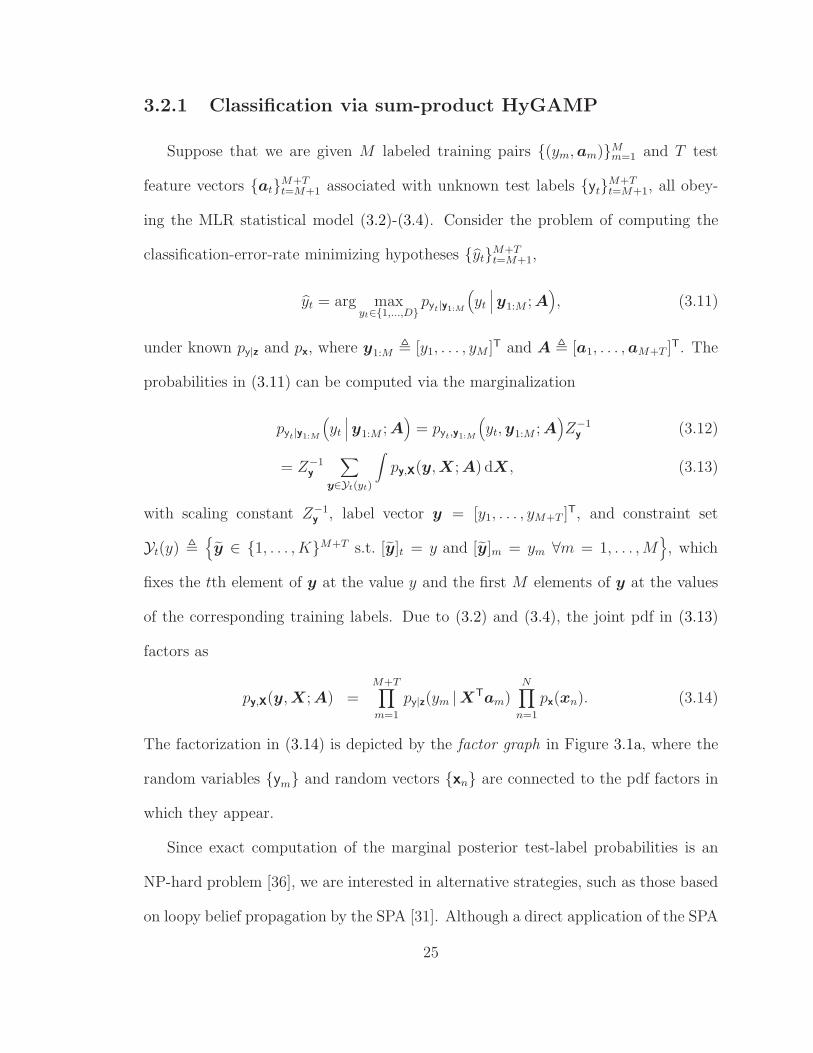
factors as

py,X(y, X; A) =M+T∏

m=1

py|z(ym |XTam)N∏

n=1

px(xn). (3.14)

The factorization in (3.14) is depicted by the factor graph in Figure 3.1a, where the

random variables {ym} and random vectors {xn} are connected to the pdf factors in

which they appear.

Since exact computation of the marginal posterior test-label probabilities is an

NP-hard problem [36], we are interested in alternative strategies, such as those based

on loopy belief propagation by the SPA [31]. Although a direct application of the SPA

25

pym|zm

pyt|zt

xnym

yt

pxn

(a) Full

pym|zm

xn

ym

pxn

(b) Reduced

Figure 3.1: Factor graph representations of (3.14), with white/gray circles denotingunobserved/observed random variables, and gray rectangles denoting pdf “factors”.

26

is itself intractable when py|z takes the MLR form (3.3), the SPA simplifies in the large-

system limit under i.i.d. sub-Gaussian A, leading to the HyGAMP approximation [13]

given4 in Table 2.1. Although in practical MLR applications A is not i.i.d. Gaussian,5

the numerical results in Section 3.5 suggest that treating it as such works sufficiently

well.

We note from Figure 3.1a that the HyGAMP algorithm is applicable to a factor

graph with vector-valued variable nodes. As such, it generalizes the GAMP algorithm

from [2], which applies only to a factor graph with scalar-variable nodes. Below,

we give a brief explanation for the steps in Table 2.1. For those interested in more

details, we suggest [13] for an overview and derivation of HyGAMP, [2] for an overview

and derivation of GAMP, [37] for rigorous analysis of GAMP under large i.i.d. sub-

Gaussian A, and [38, 39] for fixed-point and local-convergence analysis of GAMP

under arbitrary A.

Lines 19-20 of Table 2.1 produce an approximation of the posterior mean and

covariance of xn at each iteration t. Similarly, lines 8-9 produce an approximation of

the posterior mean and covariance of zm , XTam. The posterior mean and covariance

of xn are computed from the intermediate quantity rn(t), which behaves like a noisy

measurement of the true xn. In particular, for i.i.d. Gaussian A in the large-system

limit, rn(t) is a typical realization of the random vector rn = xn + vn with vn ∼

N (0, Qrn(t)). Thus, the approximate posterior pdf used in lines 19-20 is

px|r(xn|rn; Qrn) =

px(xn)N (xn; rn, Qrn)

∫px(x′

n)N (x′n; rn, Q

rn) dx′

n

. (3.15)

4 The HyGAMP algorithm in [13] is actually more general than what is specified in Table 2.1,but the version in Table 2.1 is sufficient to handle the factor graph in Figure 3.1a.

5We note that many of the standard data pre-processing techniques, such as z-scoring, tend tomake the feature distributions closer to zero-mean Gaussian.

27

A similar interpretation holds for HyGAMP’s approximation of the posterior mean

and covariance of zm in lines 8-9, which uses the intermediate vector pm(t) and the

approximate posterior pdf

pz|y,p(zm|ym, pm; Qpm)

=py|z(ym|zm)N (zm; pm, Qp

m)∫

py|z(ym|z′m)N (z′

m; pm, Qpm) dz′

m

. (3.16)

3.2.2 Classification via min-sum HyGAMP

As discussed in Section 3.1.2, an alternative approach to linear classification and

feature selection is through MAP estimation of the true weight matrix X. Given a

likelihood of the form (3.2) and a prior of the form (3.4), the MAP estimate is the

solution to the optimization problem (3.10).

Similar to how the SPA can be used to compute approximate marginal posteriors

in loopy graphs, the min-sum algorithm (MSA) [31] can be used to compute the

MAP estimate. Although a direct application of the MSA is intractable when py|z

takes the MLR form (3.3), the MSA simplifies in the large-system limit under i.i.d.

sub-Gaussian A, leading to the MSA form of HyGAMP specified in Table 2.1.

As described in Section 3.2.1, when A is large and i.i.d. sub-Gaussian, the vector

rn(t) in Table 2.1 behaves like a Gaussian-noise-corrupted observation of the true xn

with noise covariance Qrn(t). Thus, line 16 can be interpreted as MAP estimation

of xn and line 17 as measuring the local curvature of the corresponding MAP cost.

Similar interpretations hold for MAP estimation of zm via lines 5-6.

28

3.2.3 Implementation of sum-product HyGAMP

From Table 2.1, we see that HyGAMP requires inverting M + N matrices of size

K ×K (for lines 11 and 13) in addition to solving M + N joint inference problems of

dimension K in lines 16-20 and 5-9. We now briefly discuss the latter problems for

the sum-product version of HyGAMP.

Inference of xn

One choice of weight-coefficient prior pxn that facilitates row-sparse X and tractable

SPA inference is Bernoulli-multivariate-Gaussian, i.e.,

px(xn) = (1− β)δ(xn) + βN (xn; 0, vI), (3.17)

where δ(·) denotes the Dirac delta and β ∈ (0, 1]. In this case, it can be shown [14]

that the mean and variance computations in lines 19-20 of Table 2.1 reduce to

Cn = 1 +1− β

β

N (0; rn, Qrn)

N (0; rn, vI + Qrn)

(3.18)

xn = C−1n (I + v−1Qr

n)−1rn (3.19)

Qxn = C−1

n (I + v−1Qrn)−1Qr

n + (Cn − 1)xnxTn , (3.20)

which requires a K ×K matrix inversion at each n.

Inference of zm

When py|z takes the MLR form in (3.3), closed-form expressions for zm(t) and

Qzm(t) from lines 8-9 of Table 2.1 do not exist. While these computations could be

approximated using, e.g., numerical integration or importance sampling, this is expen-

sive because zm(t) and Qzm(t) must be computed for every index m at every HyGAMP

iteration t. More details on these approaches will be presented in Section 3.3.2, in

the context of SHyGAMP.

29

3.2.4 Implementation of min-sum HyGAMP

Inference of xn

To ease the computation of line 16 in Table 2.1, it is typical to choose a log-

concave prior px so that the optimization problem (3.10) is concave (since py|z in (3.3)

is also log-concave). As discussed in Section 3.1.2, a common example of a log-concave

sparsity-promoting prior is the Laplace prior (3.5). In this case, line 16 becomes

xn = arg maxx−1

2(x− rn)T[Qr

n]−1(x− rn)− λ‖x‖1, (3.21)

which is essentially the LASSO [40] problem. Although (3.21) has no closed-form

solution, it can be solved iteratively using, e.g., minorization-maximization (MM) [41].

To maximize a function J(x), MM iterates the recursion

x(t+1) = arg maxx

J(x; x(t)), (3.22)

where J(x; x) is a surrogate function that minorizes J(x) at x. In other words,

J(x; x) ≤ J(x) ∀x for any fixed x, with equality when x = x. To apply MM to

(3.21), we identify the utility function as Jn(x) , −12(x − rn)T[Qr

n]−1(x − rn) −

λ‖x‖1. Next we apply a result from [42] that established that Jn(x) is minorized by

Jn(x; x(t)n ) , −1

2(x − rn)T[Qr

n]−1(x − rn) − λ2

(xTΛ(x(t)

n )x + ‖x(t)n ‖22

)with Λ(x) ,

diag{|x1|−1, . . . , |xD|−1

}. Thus (3.22) implies

x(t+1)n = arg max

xJn(x; x(t)

n ) (3.23)

= arg maxx

xT[Qrn]−1rn −

1

2xT([Qr

n]−1 + λΛ(x(t)n ))x (3.24)

=([Qr

n]−1 + λΛ(x(t)n ))−1

[Qrn]−1rn (3.25)

where (3.24) dropped the x-invariant terms from Jn(x; x(t)n ). Note that each iteration

t of (3.25) requires a K ×K matrix inverse for each n.

30

Line 17 of Table 2.1 then says to set Qxn equal to the Hessian of the objective

function in (3.21) at xn. Recalling that the second derivative of |xnk| is undefined

when xnk = 0 but otherwise equals zero, we set Qxn = Qr

n but then zero the kth row

and column of Qxn for all k such that xnk = 0.

Inference of zm

Min-sum HyGAMP also requires the computation of lines 5-6 in Table 2.1. In our

MLR application, line 5 reduces to the concave optimization problem

zm = arg maxz−1

2(z − pm)T[Qp

m]−1(z − pm)

+ log py|z(ym|z). (3.26)

Although (3.26) can be solved in a variety of ways (see [14] for MM-based methods),

we now describe one based on Newton’s method [43], i.e.,

z(t+1)m = z(t)

m − α(t)[H(t)m ]−1g(t)

m , (3.27)

where g(t)m and H(t)

m are the gradient and Hessian of the objective function in (3.26) at

z(t)m , and α(t) ∈ (0, 1] is a stepsize. From (3.3), it can be seen that ∂

∂zilog py|z(y|z) =

δy−i − py|z(i|z), and so

g(t)m = u(z(t)

m )− eym + [Qpm]−1(z(t)

m − pm), (3.28)

where ey denotes the yth column of IK and u(z) ∈ RK×1 is defined elementwise as

[u(z)]i , py|z(i|z). (3.29)

Similarly, it is known [44] that the Hessian takes the form

H(t)m = u(z(t)

m )u(z(t)m )T − diag{u(z(t)

m )} − [Qpm]−1, (3.30)

31

which also provides the answer to line 6 of Table 2.1. Note that each iteration t of

(3.27) requires a K ×K matrix inverse for each m.

It is possible to circumvent the matrix inversion in (3.27) via componentwise

update, i.e.,

z(t+1)mk = z

(t)mk − α(t)g

(t)mk/H

(t)mk, (3.31)

where g(t)mk and H

(t)mk are the first and second derivatives of the objective function in

(3.26) with respect to zk at z = z(t)m . From (3.28)-(3.30), it follows that

g(t)mk = py|z(k|z(t)

m )− δym−k +[[Qp

m]−1]T:,k

(z(t)m − pm) (3.32)

H(t)mk = py|z(k|z(t)

m )2 − py|z(k|z(t)m )−

[[Qp

m]−1]kk

. (3.33)

3.2.5 HyGAMP summary

In summary, the SPA and MSA variants of the HyGAMP algorithm

provide tractable methods of approximating the posterior test-label proba-

bilities pyt|y1:M

(yt

∣∣∣y1:M ; A)

and computing the MAP weight matrix X =

arg maxX py1:M ,X(y1:M , X; A) respectively, under a separable likelihood (3.2) and a

separable prior (3.4). In particular, HyGAMP attacks the high-dimensional infer-

ence problems of interest using a sequence of M + N low-dimensional (in particular,

K-dimensional) inference problems and K ×K matrix inversions, as detailed in Ta-

ble 2.1.

As detailed in the previous subsections, however, these K-dimensional inference

problems are non-trivial in the sparse MLR case, making HyGAMP computationally

costly. We refer the reader to Table 3.1 for a summary of the K-dimensional inference

problems encountered in running SPA-HyGAMP or MSA-HyGAMP, as well as their

32

Algorithm Quantity Method Complexity

SPA-HyGAMP

x CF O(D3)Qx CF O(K3)z NI O(KT )Qz NI O(KDT )

MSA-HyGAMP

x MM O(TK3)Qx CF O(K3)z CWN O(TK2+K3)Qz CF O(K3)

Table 3.1: A summary of the D-dimensional inference sub-problems encounteredwhen running SPA-HyGAMP or MSA-HyGAMP, as well as their associated com-putational costs. ‘CF’ = ‘closed form’, ‘NI’ = ‘numerical integration’, ‘MM’ =‘minorization-maximization’, and ‘CWN’ = ‘component-wise Newton’s method’. Forthe NI method, T denotes the number of samples per dimension, and for the MMand CWN methods T denotes the number of iterations.

associated computational costs. Thus, in the sequel, we propose a computationally

efficient simplification of HyGAMP that, as we will see in Section 3.5, compares

favorably with existing state-of-the-art methods.

3.3 SHyGAMP for Multiclass Classification

As described in Section 3.2, a direct application of HyGAMP to sparse MLR

is computationally costly. Thus, in this section, we propose a simplified HyGAMP

(SHyGAMP) algorithm for sparse MLR, whose complexity is greatly reduced. The

simplification itself is rather straightforward: we constrain the covariance matrices

Qrn, Qx

n, Qpm, and Qz

m to be diagonal. In other words,

Qrn = diag

{qrn1, . . . , q

rnK

}, (3.34)

and similar for Qxn, Qp

m, and Qzm. As a consequence, the K ×K matrix inversions in

lines 11 and 13 of Table 2.1 each reduce to K scalar inversions. More importantly, the

33

K-dimensional inference problems in lines 16-20 and 5-9 can be tackled using much

simpler methods than those described in Section 3.2, as we detail below.

We further approximate the SHyGAMP algorithm using the scalar variance GAMP

approximation from [13], which reduces the memory and complexity of the algorithm,

which we described in detail in Section 2.4.

3.3.1 Sum-product SHyGAMP: Inference of xn

With diagonal Qrn and Qx

n, the implementation of lines 19-20 is greatly simplified

by choosing a sparsifying prior px with the separable form px(xn) =∏K

k=1 px(xnk). A

common example is the Bernoulli-Gaussian (BG) prior

px(xnk) = (1− βk)δ(xnk) + βdN (xnk; mk, vkI). (3.35)

For any separable px, lines 19-20 reduce to computing the mean and variance of the

distribution

px|r(xnk|rnk; qrnk) =

px(xnk)N (xnk ;rnk,qrnk

)∫px(x′

nk)N (x′

nk;rnk,qr

nk) dx′

nk

. (3.36)

for all n = 1 . . . N and k = 1 . . .K, as in the simpler GAMP algorithm [2]. With the

BG prior (3.35), these quantities can be computed in closed form (see, e.g., [45]).

3.3.2 Sum-product SHyGAMP: Inference of zm

With diagonal Qpm and Qz

m, the implementation of lines 8-9 can also be greatly

simplified. Essentially, the problem becomes that of computing the scalar means and

variances

zmk = C−1m

∫

RKzk py|z(ym|z)

K∏

d=1

N (zd; pmd, qpmd) dz (3.37)

qzmk = C−1

m

∫

RKz2

k py|z(ym|z)K∏

d=1

N (zd; pmd, qpmd) dz − z2

mk (3.38)

34

for m = 1 . . .M and k = 1 . . .K. Here, py|z has the MLR form in (3.3) and Cm is a

normalizing constant defined as

Cm ,∫

RKpy|z(ym|z)

K∏

d=1

N (zd; pmd, qpmd) dz. (3.39)

Note that the likelihood py|z is not separable and so inference does not decouple across

k, as it did in (3.36). We now describe several approaches to computing (3.37)-(3.38).

Numerical integration

A straightforward approach to (approximately) computing (3.37)-(3.39) is through

numerical integration (NI). For this, we propose to use a hyper-rectangular grid of

z values where, for zk, the interval[pmk − α

√qpmk, pmk + α

√qpmk

]is sampled at T

equi-spaced points. Because a K-dimensional numerical integral must be computed

for each index m and k, the complexity of this approach grows as O(MKT K), making

it impractical unless K, the number of classes, is very small.

Importance sampling

An alternative approximation of (3.37)-(3.39) can be obtained through importance

sampling (IS) [23, §11.1.4]. Here, we draw T independent samples {zm[t]}Tt=1 from

N (pm, Qpm) and compute

Cm ≈T∑

t=1

py|z(ym|zm[t]) (3.40)

zmk ≈ C−1m

T∑

t=1

zmk[t]py|z(ym|zm[t]) (3.41)

qzmk ≈ C−1

m

T∑

t=1

z2mk[t]py|z(ym|zm[t])− z2

mk (3.42)

for all m and k. The complexity of this approach grows as O(MKT ).

35

Taylor-series approximation

Another approach is to approximate the likelihood py|z using a second-order Taylor

series (TS) about pm, i.e., py|z(ym|z) ≈ fm(z; pm) with

fm(z; pm) , py|z(ym|pm) + gm(pm)T(z − pm)

+1

2(z − pm)THm(pm)(z − pm) (3.43)

for gradient gm(p) , ∂∂z

py|z(ym|z)∣∣∣z=p

and Hessian Hm(p) , ∂2

∂z2 py|z(ym|z)∣∣∣z=p

. In

this case, it can be shown [14] that

Cm ≈ fm(pm) +1

2

K∑

k=1

Hmk(pm)qpmk (3.44)

zmd ≈ C−1m

fm(pm) pmk + gmk(pm)qp

mk

+1

2

K∑

k=1

pmkqpmkHmk(pm)

(3.45)

qzmk ≈ C−1

m

fm(pm) (p2

mk + qpmk) + 2gmk(pm)pmkq

pmk

+1

2qpmk

(p2

mk + 3qpmk

)Hmk(pm)

+1

2

(p2

mk + qpmk

)Hmk(pm)

∑

k′ 6=k

qpmk′

− z2

mk, (3.46)

where Hmk(p) , [Hm(p)]kk. The complexity of this approach grows as O(MK).

Gaussian mixture approximation

It is known that the logistic cdf 1/(1+exp(−x)) is well approximated by a mixture

of a few Gaussian cdfs, which leads to an efficient method of approximating (3.37)-

(3.38) in the case of binary logistic regression (i.e., K = 2) [46]. We now develop an

extension of this method for the MLR case (i.e., K ≥ 2).

36

To facilitate the Gaussian mixture (GM) approximation, we work with the differ-

ence variables

γ(y)k ,

zy − zk k 6= y

zy k = y. (3.47)

Their utility can be seen from the fact that (recalling (3.3))

py|z(y|z) =1

1 +∑

k 6=y exp(zk − zy)(3.48)

=1

1 +∑

k 6=y exp(−γ(y)k )

, l(y)(γ(y)), (3.49)

which is smooth, positive, and bounded by 1, and strictly increasing in γ(y)k . Thus,6

for appropriately chosen {αl, µkl, σkl},

l(y)(γ) ≈L∑

l=1

αl

∏

k 6=y

Φ

(γk − µkl

σkl

), l(y)(γ), (3.50)

where Φ(x) is the standard normal cdf, σkl > 0, αl ≥ 0, and∑

l αl = 1. In practice,

the GM parameters {αl, µkl, σkl} could be designed off-line to minimize, e.g., the total

variation distance supγ∈RK |l(y)(γ)− l(y)(γ)|.

Recall from (3.37)-(3.39) that our objective is to compute quantities of the form

∫

RK(eT

k z)i py|z(y|z)N (z; p, Qp) dz , S(y)ki , (3.51)

where i ∈ {0, 1, 2}, Qp is diagonal, and ek is the kth column of IK . To exploit (3.50),

we change the integration variable to

γ(y) = T yz (3.52)

6Note that, since the role of y in l(y)(γ) is merely to ignore the yth component of the input γ,

we could have instead written l(y)(γ) = l(Jyγ) for y-invariant l(·) and Jy constructed by removingthe yth row from the identity matrix.

37

with

T y =

−Iy−1 1(y−1)×1 0(y−1)×(K−y)

01×(y−1) 1 01×(K−y)

0(K−y)×(y−1) 1(K−y)×1 −IK−y

(3.53)

to get (since det(T y) = 1)

S(y)ki =

∫

RK

(eT

k T−1y γ

)il(y)(γ)N

(γ; T yp, T yQ

pT Ty

)dγ. (3.54)

Then, applying the approximation (3.50) and

N(γ; T yp, T yQ

pT Ty

)= N

(γy; py, q

py

)

×∏

d6=y

N(γd; γy − pd, q

pd

)(3.55)

to (3.54), we find that

S(y)ki ≈

L∑

l=1

αl

∫

R

N(γy; py, q

py

)[ ∫

RK−1

(eT

k T−1y γ

)i

×∏

d6=y

N(γd; γy − pd, q

pd

)Φ

(γd − µdl

σdl

)dγd

]dγy. (3.56)

Noting that T−1y = T y, we have

eTk T −1

y γ =

γy − γk k 6= y

γy k = y. (3.57)

Thus, for a fixed value of γy = c, the inner integral in (3.56) can be expressed as a

product of linear combinations of terms

∫

R

γiN(γ; c− p, q

)Φ

(γ − µ

σ

)dγ , Ti (3.58)

with i ∈ {0, 1, 2}, which can be computed in closed form. In particular, defining

x , c−p−µ√σ2+q

, we have

T0 = Φ(x) (3.59)

T1 = (c− p)Φ(x) +qφ(x)√σ2 + q

(3.60)

T2 =(T1)

2

Φ(x)+ qΦ(x)− q2φ(x)

σ2 + q

(x +

φ(x)

Φ(x)

), (3.61)

38

which can be obtained using the results in [47, §3.9]. The outer integral in (3.56) can

then be approximated via numerical integration.

If a grid of T values is used for numerical integration over γy in (3.56), then the

overall complexity of the method grows as O(MKLT ). Our experiments indicate

that relatively small values (e.g., L = 2 and T = 7) suffice.

Performance comparison

Above we described four methods of approximating lines 8-9 in Table 2.1 under

diagonal Qp and Qz. We now compare the accuracy and complexity of these meth-

ods. In particular, we measured the accuracy of the conditional mean (i.e., line 8)

approximation as follows (for a given p and Qp):

1. generate i.i.d. samples ztrue[t] ∼ N (z; p, Qp) and ytrue[t] ∼ py|z(y | ztrue[t]) for

t = 1 . . . T ,

2. compute the approximation z[t] ≈ E{z | y = ytrue[t], p = p; Qp} using each

method described in Sections 3.3.2–3.3.2,

3. compute average MSE , 1T

∑Tt=1

∥∥∥ztrue[t]− z[t]∥∥∥2

2for each method,

and we measured the combined runtime of lines 8-9 for each method. Unless otherwise

noted, we used K = 4 classes, p = e1, Qp = qpIK , and qp = 1 in our experiments. For

numerical integration (NI), we used a grid of size T = 7 and radius of α = 4 standard

deviations; for importance sampling (IS), we used T = 1500 samples; and for the

Gaussian-mixture (GM) method, we used L = 2 mixture components and a grid size

of T = 7. Empirically, we found that smaller grids or fewer samples compromised

accuracy, whereas larger grids or more samples compromised runtime.

39

Figure 3.2 plots the normalized MSE versus variance qp for the four methods under

test, in addition to the trivial method z[t] = p. The figure shows that the NI, IS, and

GM methods performed similarly across the full range of qp and always outperform

the trivial method. The Taylor-series method, however, breaks down when qp > 1. A

close examination of the figure reveals that GM gave the best accuracy, IS the second

best accuracy, and NI the third best accuracy.

Figure 3.3 shows the cumulative runtime (over M = 500 training samples) of the

methods from Sections 3.3.2–3.3.2 versus the number of classes, K. Although the

Taylor-series method was the fastest, we saw in Figure 3.2 that it is accurate only

at small variances qp. Figure 3.3 then shows GM was about an order-of-magnitude

faster than IS, which was several orders-of-magnitude faster than NI.

Together, Figures 3.2-3.3, show that our proposed GM method dominated the IS

and NI methods in both accuracy and runtime. Thus, for the remainder of the paper,

we implement sum-product SHyGAMP using the GM method from Section 3.3.2.

3.3.3 Min-sum SHyGAMP: Inference of xn

With diagonal Qrn and Qx

n, the implementation of lines 16-17 in Table 2.1 can be

significantly simplified. Recall that, when the prior px is chosen as i.i.d. Laplace (3.5),

line 16 manifests as (3.21), which is in general a non-trivial optimization problem.

But with diagonal Qrn, (3.21) decouples into K instances of the scalar optimization

xnk = arg maxx−1

2

(x− rnk)2

qrnk

− λ|x|, (3.62)

which is known to have the closed-form “soft thresholding” solution

xnk = sgn(rnk) max{0, |rnk| − λqrnk}. (3.63)

40

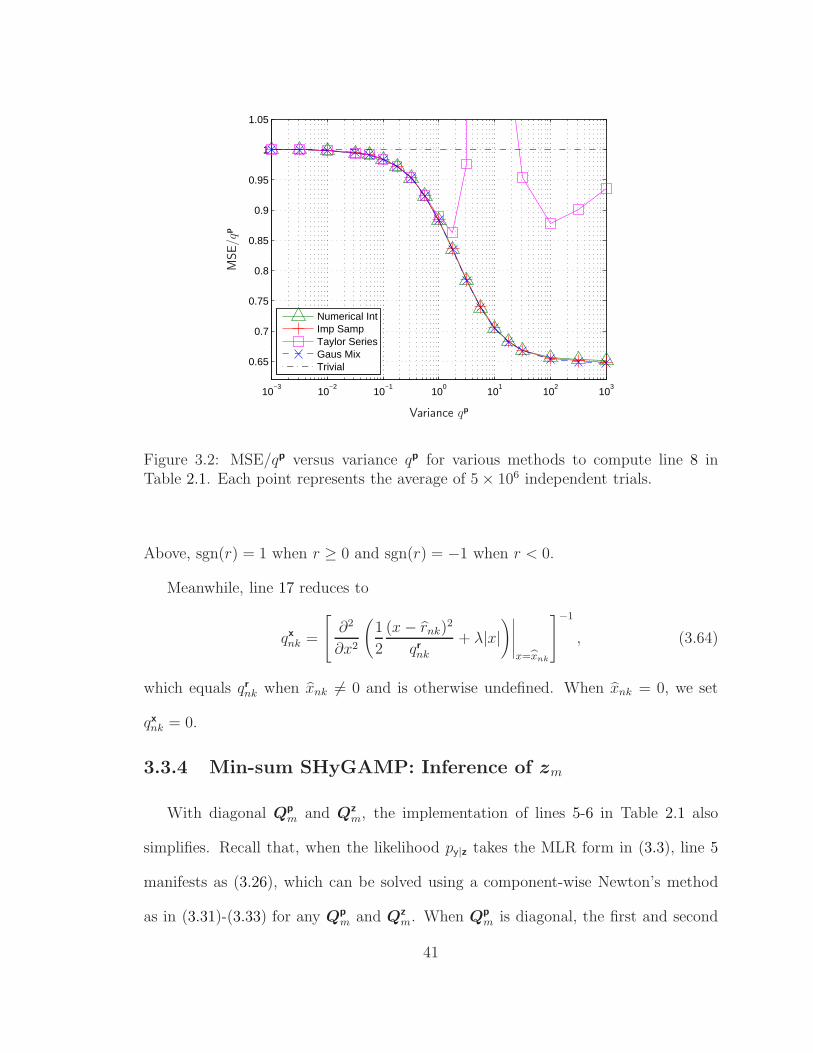
10−3

10−2

10−1

100

101

102

103

0.65

0.7

0.75

0.8

0.85

0.9

0.95

1

1.05

Numerical IntImp SampTaylor SeriesGaus MixTrivial

Variance qp

MSE/q

p

Figure 3.2: MSE/qp versus variance qp for various methods to compute line 8 inTable 2.1. Each point represents the average of 5× 106 independent trials.

Above, sgn(r) = 1 when r ≥ 0 and sgn(r) = −1 when r < 0.

Meanwhile, line 17 reduces to

qxnk =

∂2

∂x2

(1

2

(x− rnk)2

qrnk

+ λ|x|)∣∣∣∣∣

x=xnk

−1

, (3.64)

which equals qrnk when xnk 6= 0 and is otherwise undefined. When xnk = 0, we set

qxnk = 0.

3.3.4 Min-sum SHyGAMP: Inference of zm

With diagonal Qpm and Qz

m, the implementation of lines 5-6 in Table 2.1 also

simplifies. Recall that, when the likelihood py|z takes the MLR form in (3.3), line 5

manifests as (3.26), which can be solved using a component-wise Newton’s method

as in (3.31)-(3.33) for any Qpm and Qz

m. When Qpm is diagonal, the first and second

41

100

101

102

10−4

10−3

10−2

10−1

100

101

Numerical Int.Imp. SamplingTaylor SeriesGaus. Mixture

Runtim

e[s

ec]

Number of Classes K

Figure 3.3: Cumulative runtime (over M = 500 samples) versus number-of-classesK for various methods to compute lines 8-9 in Table 2.1. Each point represents theaverage of 2000 independent trials.

derivatives (3.32)-(3.33) reduce to

g(k)mk = py|z(k|z(t)

m )− δym−k + (z(t)mk − pmk)/q

pmk. (3.65)

H(t)mk = py|z(k|z(t)

m )2 − py|z(k|z(t)m )− 1/qp

mk, (3.66)

which leads to a reduction in complexity.

Furthermore, line 6 simplifies, since with diagonal Qzm it suffices to compute only

the diagonal components of H (t)m in (3.30). In particular, when Qp

m is diagonal, the

result becomes

qzmk =

1

1/qpmk + py|z(k|zm)− py|z(k|zm)2

. (3.67)

42

Algorithm Quantity Method Complexity

SPA-SHyGAMP

x CF O(K)Qx CF O(K)z GM O(KLT )Qz GM O(KLT )

MSA-SHyGAMP

x ST O(D)Qx CF O(K)z CWN O(KT )Qz CF O(K3)

Table 3.2: A summary of the K-dimensional inference sub-problems encounteredwhen running SPA-SHyGAMP or MSA-SHyGAMP, as well as their associated com-putational costs. ‘CF’ = ‘closed form’, ‘GM’ = ‘Gaussian mixture’, ‘ST’ = ‘Soft-thresholding’, and ‘CWN’ = ‘component-wise Newton’s method’. For the GM, Ldenotes the number of mixture components and T the number of samples in the 1Dnumerical integral, and for CWN T denotes the number of iterations.

Algorithm HyGAMP SHyGAMPDiagonal covariance matrices XSimplified K-dimensional inference XScalar-variance approximation XOnline parameter tuning X

Table 3.3: High-level comparison of SHyGAMP and HyGAMP.

3.3.5 SHyGAMP summary

In summary, by approximating the covariance matrices as diagonal, the SPA-

SHyGAMP and MSA-SHyGAMP algorithms improve computationally upon their

HyGAMP counterparts. A summary of the K-dimensional inference problems en-

countered when running SPA-SHyGAMP or MSA-SHyGAMP, as well as their asso-

ciated computational costs, is given in Table 3.2. A high-level comparison between

HyGAMP and SHyGAMP is given in Table 3.3.

43

3.4 Online Parameter Tuning

The weight vector priors in (3.5) and (3.35) depend on modeling parameters that,

in practice, must be tuned. Although cross-validation (CV) is the customary ap-

proach to tuning such model parameters, it can be very computationally costly, since

each parameter must be tested over a grid of hypothesized values and over multiple

data folds. For example, K-fold7 cross-validation tuning of P parameters using G

hypothesized values of each parameter requires the training and evaluation of KGP

classifiers.

3.4.1 Parameter selection for Sum-product SHyGAMP

For SPA-SHyGAMP, we propose to use the zero-mean Bernoulli-Gaussian prior

in (3.35), which has parameters βk, mk, and vk. Instead of CV, we use the EM-GM-

AMP framework described in [4] to tune these parameters online. See [14] for details

regarding the initialization of βk, mk, and vk.

3.4.2 Parameter selection for Min-sum SHyGAMP

To use MSA-SHyGAMP with the Laplacian prior in (3.5), we need to specify the

scale parameter λ. For this, we use a modification of the SURE-AMP framework

from [35], which adjusts λ to minimize the Stein’s unbiased risk estimate (SURE) of

the weight-vector MSE.

We describe our method by first reviewing SURE and SURE-AMP. First, suppose

that the goal is to estimate the value of x, which is a realization of the random variable

7This K has no relation to the number of classes.

44

x, from the noisy observation r, which is a realization of

r = x +√

qrw, (3.68)

with w ∼ N (0, 1) and qr > 0. For this purpose, consider an estimate of the form

x = f(r, qr; θ) where θ contains tunable parameters. For convenience, define the

shifted estimation function g(r, qr; θ) , f(r, qr; θ)− r and its derivative g′(r, qr; θ) ,

∂∂r

g(r, qr; θ). Then Stein [48] established the following result on the mean-squared

error, or risk, of the estimate x:

E{[x− x]2

}= qr + E

{g2(r, qr; θ) + 2qrg′(r, qr; θ)

}. (3.69)

The implication of (3.69) is that, given only the noisy observation r and the noise

variance qr, one can compute an estimate

SURE(r, qr; θ) , qr + g2(r, qr; θ) + 2qrg′(r, qr; θ) (3.70)

of the MSE(θ) , E{[x− x]2

}that is unbiased, i.e.,

E{SURE(r, qr; θ)

}= MSE(θ). (3.71)

These unbiased risk estimates can then be used as a surrogate for the true MSE when

tuning θ.

In [35], it was noticed that the assumption (3.68) is satisfied by AMP’s denoiser

inputs {rn}Nn=1, and thus [35] proposed to tune the soft threshold λ to minimize the

SURE:

λ = arg minλ

N∑

n=1

g2(rn, qr; λ) + 2qrg′(rn, q

r; λ). (3.72)

45

Recalling the form of the estimator f(·) from (3.63), we have

g2(rn, qr; λ) =

λ2(qr)2 if |rn| > λqr

r2n otherwise

(3.73)

g′(rn, qr; λ) =

−1 if |rn| < λqr

0 otherwise. (3.74)

However, solving (3.72) for λ is non-trivial because the objective is non-smooth and

has many local minima. A stochastic gradient descent approach was proposed in [35],

but its convergence speed is too slow to be practical.

Since (3.68) also matches the scalar-variance SHyGAMP model from Section 2.4,

we propose to use SURE to tune λ for min-sum SHyGAMP. But, instead of the

empirical average in (3.72), we propose to use a statistical average, i.e.,

λ = arg minλ

E{g2(r, qr; λ) + 2qrg′(r, qr; λ)

}

︸︷︷︸, J(λ)

, (3.75)

by modeling the random variable r as a Gaussian mixture (GM) whose parameters

are fitted to {rnk}. As a result, the objective in (3.75) is smooth. Moreover, by

constraining the smallest mixture variance to be at least qr, the objective becomes

unimodal, in which case λ from (3.75) is the unique root of ddλ

J(λ). To find this

root, we use the bisection method. In particular, due to (3.73)-(3.74), the objective

in (3.75) becomes

J(λ) =∫ −λqr

−∞pr(r)λ

2(qr)2 dr +∫ λqr

−λqrpr(r)(r

2 − 2qr) dr

+∫ ∞

λqrpr(r)λ

2(qr)2 dr, (3.76)

from which it can be shown that [14]

d

dλJ(λ) = 2λ(qr)2

[1− Pr{−λqr < r < λqr}

]

−[pr(λqr) + pr(−λqr)

]2(qr)2. (3.77)

46

For GM fitting, we use the standard EM approach [23] and find that relatively few

(e.g., L = 3) mixture terms suffice. Note that we re-tune λ using the above technique

at each iteration of Table 2.1, immediately before line 16. Experimental verification

of our method is provided in Section 3.5.2.

3.5 Numerical Experiments

In this section we describe the results of several experiments used to test SHyGAMP.

In these experiments, EM-tuned SPA-SHyGAMP and SURE-tuned MSA-SHyGAMP

were compared to two state-of-the-art sparse MLR algorithms: SBMLR [27] and

GLMNET [26]. We are particularly interested in SBMLR and GLMNET because

[26,27] show that they have strong advantages over earlier algorithms, e.g., [10,24,25].

As described in Section 3.1.2, both SBMLR and GLMNET use ℓ1 regularization, but

SBMLR tunes the regularization parameter λ using evidence maximization while

GLMNET tunes it using cross-validation (using the default value of 10 folds unless

otherwise noted). For SBMLR and GLMNET, we ran code written by the authors 8 9

under default settings (unless otherwise noted). For SHyGAMP, we used the damping

modification described in [39]. We note that the runtimes reported for all algorithms

include the total time spent to tune all parameters and train the final classifier.

Due to space limitations, we do not show the performance of the more compli-

cated HyGAMP algorithm from Section 3.2. However, our experience suggests that

HyGAMP generates weight matrices X that are very similar to those generated by

SHyGAMP, but with much longer runtimes, especially as K grows.

8SBMLR obtained from http://theoval.cmp.uea.ac.uk/matlab/

9GLMNET obtained from http://www.stanford.edu/~hastie/glmnet_matlab/

47

http://theoval.cmp.uea.ac.uk/matlab/

http://www.stanford.edu/~hastie/glmnet_matlab/

3.5.1 Synthetic data in the M ≪ N regime

We first describe the results of three experiments with synthetic data. For these

experiments, the training data were randomly generated and algorithm performance

was averaged over several data realizations. In all cases, we started with balanced

training labels ym ∈ {1, . . . , K} for m = 1, . . . , M (i.e., M/K examples from each of

K classes). Then, for each data realization, we generated M i.i.d. training features am

from the class-conditional generative distribution am | ym ∼ N (µym, vIN). In doing

so, we chose the intra-class variance, v, to attain a desired Bayes error rate (BER)

of 10% (see [14] for details), and we used randomly generated S-sparse orthonormal

class means, µk ∈ RN . In particular, we generated [µ1, . . . , µK ] by drawing a S × S

matrix with i.i.d.N (0, 1) entries, performing a singular value decomposition, and zero-

padding the first K left singular vectors to length N . We note that our generation of

y, A, X is matched [49] to the multinomial logistic model (3.2)-(3.3).

Given a training data realization, each algorithm was invoked to yield a weight

matrix X = [x1, . . . , xK ]. The corresponding expected test-error rate was then ana-

lytically computed as

Pr{err} = 1− 1

K

K∑

y=1

Pr{cor|y} (3.78)

Pr{cor|y} = Pr⋂

k 6=y

{(xy − xk)

Ta < (xy − xk)Tµy

}, (3.79)

where a ∼ N (0, vIN) and the multivariate normal cdf in (3.79) was computed using

Matlab’s mvncdf.

For all three synthetic-data experiments, we used K = 4 classes and S ≪ M ≪ N .

In the first experiment, we fixed S and N and we varied M ; in the second experiment,

we fixed N and M and we varied S; and in the third experiment, we fixed S and M

48

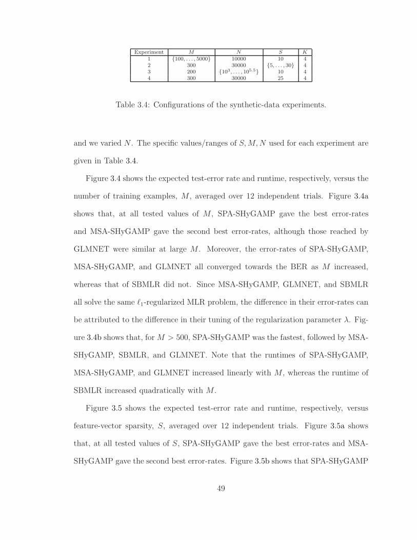
Experiment M N S K1 {100, . . . , 5000} 10000 10 42 300 30000 {5, . . . , 30} 43 200 {103, . . . , 105.5} 10 44 300 30000 25 4

Table 3.4: Configurations of the synthetic-data experiments.

and we varied N . The specific values/ranges of S, M, N used for each experiment are

given in Table 3.4.

Figure 3.4 shows the expected test-error rate and runtime, respectively, versus the

number of training examples, M , averaged over 12 independent trials. Figure 3.4a

shows that, at all tested values of M , SPA-SHyGAMP gave the best error-rates

and MSA-SHyGAMP gave the second best error-rates, although those reached by

GLMNET were similar at large M . Moreover, the error-rates of SPA-SHyGAMP,

MSA-SHyGAMP, and GLMNET all converged towards the BER as M increased,

whereas that of SBMLR did not. Since MSA-SHyGAMP, GLMNET, and SBMLR

all solve the same ℓ1-regularized MLR problem, the difference in their error-rates can

be attributed to the difference in their tuning of the regularization parameter λ. Fig-

ure 3.4b shows that, for M > 500, SPA-SHyGAMP was the fastest, followed by MSA-

SHyGAMP, SBMLR, and GLMNET. Note that the runtimes of SPA-SHyGAMP,

MSA-SHyGAMP, and GLMNET increased linearly with M , whereas the runtime of

SBMLR increased quadratically with M .

Figure 3.5 shows the expected test-error rate and runtime, respectively, versus

feature-vector sparsity, S, averaged over 12 independent trials. Figure 3.5a shows

that, at all tested values of S, SPA-SHyGAMP gave the best error-rates and MSA-

SHyGAMP gave the second best error-rates. Figure 3.5b shows that SPA-SHyGAMP

49

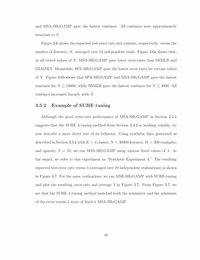
and MSA-SHyGAMP gave the fastest runtimes. All runtimes were approximately

invariant to S.

Figure 3.6 shows the expected test-error rate and runtime, respectively, versus the

number of features, N , averaged over 12 independent trials. Figure 3.6a shows that,

at all tested values of N , MSA-SHyGAMP gave lower error-rates than SBMLR and

GLMNET. Meanwhile, SPA-SHyGAMP gave the lowest error-rates for certain values

of N . Figure 3.6b shows that SPA-SHyGAMP and MSA-SHyGAMP gave the fastest

runtimes for N ≥ 10000, while SBMLR gave the fastest runtimes for N ≤ 3000. All

runtimes increased linearly with N .

3.5.2 Example of SURE tuning

Although the good error-rate performance of MSA-SHyGAMP in Section 3.5.1

suggests that the SURE λ-tuning method from Section 3.4.2 is working reliably, we

now describe a more direct test of its behavior. Using synthetic data generated as

described in Section 3.5.1 with K = 4 classes, N = 30000 features, M = 300 examples,

and sparsity S = 25, we ran MSA-SHyGAMP using various fixed values of λ. In

the sequel, we refer to this experiment as “Synthetic Experiment 4.” The resulting

expected test-error rate versus λ (averaged over 10 independent realizations) is shown

in Figure 3.7. For the same realizations, we ran MSE-SHyGAMP with SURE-tuning

and plot the resulting error-rate and average λ in Figure 3.7. From Figure 3.7, we

see that the SURE λ-tuning method matched both the minimizer and the minimum

of the error-versus-λ trace of fixed-λ MSA-SHyGAMP.

50

102

103

0.1

0.12

0.14

0.16

0.18

0.2

SPA SHyGAMPMSA SHyGAMPSBMLRGLMNETBER

Tes

tErr

orRat

e

Number of Training Samples M

(a) Error

102

103

100

101

102

103

SPA SHyGAMPMSA SHyGAMPSBMLRGLMNET

Runtim

e[s

ec]


(b) Runtime

Figure 3.4: Synthetic Experiment 1: expected test-error rate and runtime versus M .Here, K = 4, N = 10000, and S = 10.

51

5 10 15 20 25 30

0.1

0.12

0.14

0.16

0.18

0.2

0.22


Tes

tErr

orRat

e

True Sparsity S

(a) Error

5 10 15 20 25 3010

0

101

102


Runtim

e[s

ec]

True Sparsity S

(b) Runtime

Figure 3.5: Synthetic Experiment 2: expected test-error rate and runtime versus S.Here, K = 4, M = 300, and N = 30000.

52

103

104

105

0.09

0.1

0.11

0.12

0.13

0.14

0.15

0.16

0.17

0.18


Tes

tErr

orRat

e

Number of Features N

(a) Error

103

104

105

10−1

100

101

102

103


Runtim

e[s

ec]

Number of Features N

(b) Runtime

Figure 3.6: Synthetic Experiment 3: expected test-error rate and runtime versus N .Here, K = 4, M = 200, and S = 10.

53

100

101

102

0.16

0.18

0.2

0.22

0.24

0.26

0.28

0.3

0.32

FixedSURE

Tes

tErr

orRat

e

Regularization Parameter λ

Figure 3.7: Synthetic experiment 4: expected test-error rate versus regularizationparameter λ for fixed-λ MSA-SHyGAMP. Here, K = 4, M = 300, N = 30000, andS = 25. Also shown is the average test-error rate for SURE-tuned MSA-SHyGAMPplotted at the average value of λ.

3.5.3 Micro-array gene expression

Next we consider classification and feature-selection using micro-array gene expres-

sion data. Here, the labels indicate which type of disease is present (or no disease)

and the features represent gene expression levels. The objective is i) to determine

which subset of genes best predicts the various diseases and ii) to classify whether an

(undiagnosed) patient is at risk for any of these diseases based on their gene profile.

We tried two datasets: one from Sun et al. [15] and one from Bhattacharjee

et al. [16]. The Sun dataset includes M = 179 examples, N = 54613 features, and

K = 4 classes; and the Bhattacharjee dataset includes M = 203 examples, N = 12600

54

features, and K = 5 classes. With the Sun dataset, we applied a log2(·) transformation

and z-scored prior to processing, while with Bhattacharjee we simply z-scored (since

the dataset included negative values).

The test-error rate was estimated as follows for each dataset. We consider a

total of T “trials.” For the tth trial, we i) partition the dataset into a training

subset of size Mtrain,t and a test subset of size Mtest,t, ii) design the classifier using

the training subset, and iii) apply the classifier to the test subset, recording the

test errors {etm}Mtest,t

m=1 , where etm ∈ {0, 1} indicates whether the mth example was

in error. We then estimate the average test-error rate using the empirical average

µ , M−1test

∑Tt=1

∑Mtest,t

m=1 etm, where Mtest =∑T

t=1 Mtest,t. If the test sets are constructed

without overlap, we can model {etm} as i.i.d. Bernoulli(µ), where µ denotes the true

test-error rate. Then, since µ is Binomial(µ, Mtest), the standard deviation (SD) of

our error-rate estimate µ is√

var{µ} =√

µ(1− µ)/Mtest. Since µ is unknown, we

approximate the SD by√

µ(1− µ)/Mtest.

Tables 3.5 and 3.6 show, for each algorithm, the test-error rate estimate µ, the ap-

proximate SD√

µ(1− µ)/Mtest of the estimate, the average runtime, and two metrics

for the sparsity of X. The ‖X‖0 metric quantifies the number of non-zero entries in

X (i.e., absolute sparsity), while the S99 metric quantifies the number of entries of X

needed to reach 99% of the Frobenius norm of X (i.e., effective sparsity). We note that

the reported values of S99 and ‖X‖0 represent the average over the T folds. For both

the Sun and Bhattacharjee datasets, we used T = 19 trials and Mtest,t = ⌊M/20⌋ ∀t.

Table 3.5 shows results for the Sun dataset. There we see that MSA-SHyGAMP

gave the best test-error rate, although the other algorithms were not far behind and all

error-rate estimates were within the estimator standard deviation. SPA-SHyGAMP

55

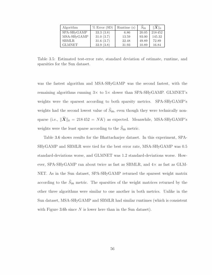
Algorithm % Error (SD) Runtime (s) S99 ‖X‖0SPA-SHyGAMP 33.3 (3.8) 6.86 20.05 218 452MSA-SHyGAMP 31.0 (3.7) 13.59 93.00 145.32SBMLR 31.6 (3.7) 22.48 49.89 72.89GLMNET 33.9 (3.8) 31.93 10.89 16.84

Table 3.5: Estimated test-error rate, standard deviation of estimate, runtime, andsparsities for the Sun dataset.

was the fastest algorithm and MSA-SHyGAMP was the second fastest, with the

remaining algorithms running 3× to 5× slower than SPA-SHyGAMP. GLMNET’s

weights were the sparsest according to both sparsity metrics. SPA-SHyGAMP’s

weights had the second lowest value of S99, even though they were technically non-

sparse (i.e., ‖X‖0 = 218 452 = NK) as expected. Meanwhile, MSA-SHyGAMP’s

weights were the least sparse according to the S99 metric.

Table 3.6 shows results for the Bhattacharjee dataset. In this experiment, SPA-

SHyGAMP and SBMLR were tied for the best error rate, MSA-SHyGAMP was 0.5

standard-deviations worse, and GLMNET was 1.2 standard-deviations worse. How-

ever, SPA-SHyGAMP ran about twice as fast as SBMLR, and 4× as fast as GLM-

NET. As in the Sun dataset, SPA-SHyGAMP returned the sparsest weight matrix

according to the S99 metric. The sparsities of the weight matrices returned by the

other three algorithms were similar to one another in both metrics. Unlike in the

Sun dataset, MSA-SHyGAMP and SBMLR had similar runtimes (which is consistent

with Figure 3.6b since N is lower here than in the Sun dataset).

56

Algorithm % Error (SD) Runtime (s) S99 ‖X‖0SPA-SHyGAMP 9.5 (2.1) 3.26 16.15 63 000MSA-SHyGAMP 10.5 (2.2) 6.11 55.20 84.65SBMLR 9.5 (2.1) 6.65 44.25 79.10GLMNET 12.0 (2.4) 13.67 49.65 89.40

Table 3.6: Estimated test-error rate, standard deviation of estimate, runtime, andsparsities for the Bhattacharjee dataset.

3.5.4 Text classification with the RCV1 dataset

Next we consider text classification using the Reuter’s Corpus Volume 1 (RCV1)

dataset [20]. Here, each sample (ym, am) represents a news article, where ym indicates

the article’s topic and am indicates the frequencies of common words in the article.

The version of the dataset that we used10 contained N = 47 236 features and 53 topics.

However, we used only the first K = 25 of these topics (to reduce the computational

demand). Also, we retained the default training and test partitions, which resulted

in the use of M = 14 147 samples for training and 469 571 samples for testing.

The RCV1 features are very sparse (only 0.326% of the features are non-zero) and

non-negative, which conflicts with the standard assumptions used for the derivation

of AMP algorithms: that A is i.i.d. zero-mean and sub-Gaussian. Interestingly, the

RCV1 dataset also caused difficulties for SBMLR, which diverged under default set-

tings. This divergence was remedied by decreasing the value of a step-size parameter11

to 0.1 from the default value of 1.

10http://www.csie.ntu.edu.tw/~cjlin/libsvmtools/datasets/multiclass.html

11See the variable scale on lines 129 and 143 of sbmlr.m.

57

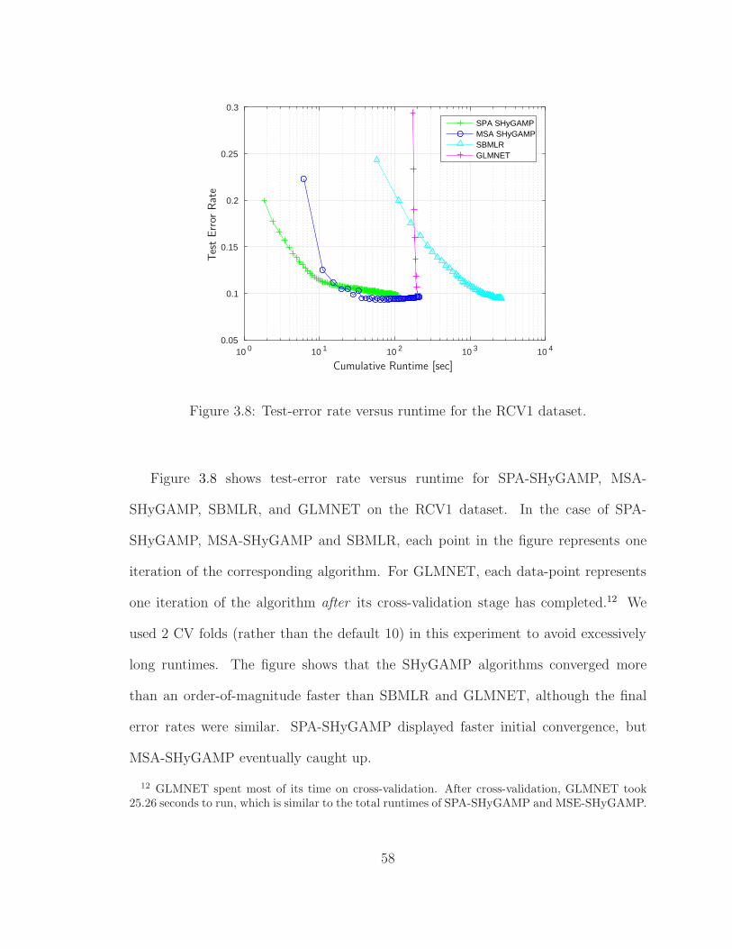
http://www.csie.ntu.edu.tw/~cjlin/libsvmtools/datasets/multiclass.html

10 0 10 1 10 2 10 3 10 40.05

0.1

0.15

0.2

0.25

0.3


Tes

tErr

orRat

e

Cumulative Runtime [sec]

Figure 3.8: Test-error rate versus runtime for the RCV1 dataset.

Figure 3.8 shows test-error rate versus runtime for SPA-SHyGAMP, MSA-

SHyGAMP, SBMLR, and GLMNET on the RCV1 dataset. In the case of SPA-

SHyGAMP, MSA-SHyGAMP and SBMLR, each point in the figure represents one

iteration of the corresponding algorithm. For GLMNET, each data-point represents

one iteration of the algorithm after its cross-validation stage has completed.12 We

used 2 CV folds (rather than the default 10) in this experiment to avoid excessively

long runtimes. The figure shows that the SHyGAMP algorithms converged more

than an order-of-magnitude faster than SBMLR and GLMNET, although the final

error rates were similar. SPA-SHyGAMP displayed faster initial convergence, but

MSA-SHyGAMP eventually caught up.

12 GLMNET spent most of its time on cross-validation. After cross-validation, GLMNET took25.26 seconds to run, which is similar to the total runtimes of SPA-SHyGAMP and MSE-SHyGAMP.

58

3.5.5 MNIST handwritten digit recognition

Finally, we consider handwritten digit recognition using the Mixed National In-

stitute of Standards and Technology (MNIST) dataset [50]. This dataset consists of

70 000 examples, where each example is an N = 784 pixel image of one of K = 10

digits between 0 and 9. These features were again non-negative, which conflicts with

the standard AMP assumption of i.i.d. zero-mean A.

Our experiment characterized test-error rate versus the number of training exam-

ples, M , for the SPA-SHyGAMP, MSA-SHyGAMP, SBMLR, and GLMNET algo-

rithms. For each value of M , we performed 50 Monte-Carlo trials. In each trial, M

training samples were selected uniformly at random and the remainder of the data

were used for testing. Figure 3.9 shows the average estimated test-error rate µ versus

the number of training samples, M , for the algorithms under test. The error-bars in

the figure correspond to the average of the per-trial estimated SD over the 50 trials.

For SBMLR, we reduced the stepsize to 0.5 from the default value of 1 to prevent a

significant degradation of test-error rate. The figure shows SPA-SHyGAMP attaining

significantly better error-rates than the other algorithms at small values of M (and

again at the largest value of M considered for the plot). For this plot, M was chosen

to focus on the M < N regime.

3.6 Conclusion

For the problem of multi-class linear classification and feature selection, we pro-

posed several AMP-based approaches to sparse multinomial logistic regression. We

started by proposing two algorithms based on HyGAMP [13], one of which finds the

59

10 2 10 30.15

0.2

0.25

0.3

0.35

0.4

0.45SPA SHyGAMPMSA SHyGAMPSBMLRGLMNET

Tes

tErr

orRat

e


Figure 3.9: Estimated test-error rate versus M for the MNIST dataset, with error-barsindicating the standard deviation of the estimate.

maximum a posteriori (MAP) linear classifier based on the multinomial logistic like-

lihood and a Laplacian prior, and the other of which finds an approximation of the

test-error-rate minimizing linear classifier based on the multinomial logistic likelihood

and a Bernoulli-Gaussian prior. The numerical implementation of these algorithms

is challenged, however, by the need to solve K-dimensional inference problems of

multiplicity M at each HyGAMP iteration. Thus, we proposed simplified HyGAMP

(SHyGAMP) approximations based on a diagonalization of the message covariances

and a careful treatment of the K-dimensional inference problems. In addition, we de-

scribed EM- and SURE-based methods to tune the hyperparameters of the assumed

60

statistical model. Finally, using both synthetic and real-world datasets, we demon-

strated improved error-rate and runtime performance relative to the state-of-the-art

SBMLR [26] and GLMNET [27] approaches to sparse MLR.

61

Chapter 4: Sketched Clustering via Approximate Message

Passing

4.1 Introduction

In this chapter13 we consider the problem of sketched clustering. Given a dataset

D , [d1, . . . , dT ] ∈ RN×T comprising T samples of dimension N , the standard clus-

tering problem is to find K centroids X , [x1, . . . , xK ] ∈ RN×K that minimize the

sum of squared errors (SSE)

SSE(D, X) ,1

T

T∑

t=1

mink‖dt − xk‖22. (4.1)

Finding the optimal X is an NP-hard problem [51]. Thus, many heuristic approaches

have been proposed, such as the k-means algorithm [52,53]. Because k-means can get

trapped in bad local minima, robust variants have been proposed, such as k-means++

[54], which uses a careful random initialization procedure to yield solutions with

SSE that have on average ≤ 8(lnK + 2) times the minimal SSE. The computational

complexity of k-means++ scales as O(TKNI), with I the number of iterations, which

is impractical when T is large.

13The content from this chapter is largely excerpted from the manuscript co-authored with AntoineChatalic, Remi Gribonval, and Philip Schniter, titled “Sketched Clustering via Hybrid ApproximateMessage Passing.”

62

4.1.1 Sketched Clustering

In sketched clustering [55–57], the dataset D is first sketched down to a vector

y with M = O(KN) components, from which the centroids X are subsequently

extracted. In the typical case that K ≪ T , the sketch consumes much less memory

than the original dataset. If the sketch can be performed efficiently, then—since the

complexity of centroid-extraction is invariant to T—sketched clustering may be more

efficient than direct clustering methods when T is large. Note, for example, that

k-means++ processes the T data samples in D at every iteration, whereas sketched

clustering processes the T data samples in D only once, during the sketching step.

In this work, we focus on sketches of the type proposed by Keriven et al. in [55,56],

which use y = [y1, . . . , yM ]T with

ym =1

T

T∑

t=1

exp(jwTmdt) (4.2)

and randomly generated W , [w1, . . . , wM ]T ∈ RM×N . Note that ym in (4.2) can be

interpreted as a sample of the empirical characteristic function [58], i.e.,

φ(wm) =∫

RNp(d) exp(jwT

md) dd (4.3)

under the empirical distribution p(d) = 1T

∑Tt=1 δ(d − dt), with Dirac δ(·). Here,

each wm can be interpreted as a multidimensional frequency sample. The process of

sketching D down to y via (4.2) costs O(TMN) operations, but it can be performed

efficiently in an online and/or distributed manner.

To recover the centroids X from y, the state-of-the-art algorithm is compressed

learning via orthogonal matching pursuit with replacement (CL-OMPR) [55, 56]. It

63

aims to solve

arg minX

minα:1Tα=1

M∑

m=1

∣∣∣∣∣ym −K∑

k=1

αk exp(jwTmxk)

∣∣∣∣∣

2

(4.4)

using a greedy heuristic inspired by the orthogonal matching pursuit (OMP) algorithm

[59] popular in compressed sensing. With sketch length M ≥ 10KN , CL-OMPR

typically recovers centroids of similar or better quality to those attained with k-

means++. One may wonder, however, whether it is possible to recover accurate

centroids with sketch lengths closer to the counting bound M = KN . Also, since

CL-OMPR’s computational complexity is O(MNK2), one may wonder whether it is

possible to recover accurate centroids with computational complexity O(MNK).

4.1.2 Contributions

To recover the centroids X from a sketch y of the form in (4.2), we propose the

compressive learning via approximate message passing (CL-AMP) algorithm, with

computational complexity O(MNK). Numerical experiments show that CL-AMP

accurately recovers centroids from sketches of length M = 2KN in most cases, which

is an improvement over CL-OMPR. Experiments also show that CL-AMP recovers

centroids faster and more accurately than k-means++ in certain operating regimes,

such as when T is large.

The remainder of this chapter is organized as follows. In Section 4.2, we derive CL-

AMP after reviewing relevant background on approximate message passing (AMP)

algorithms. In Section 4.3, we present numerical experiments using synthetic and

MNIST data, and we apply CL-AMP to multidimensional frequency estimation. In

Section 4.4, we conclude.

64

4.2 Compressive Learning via AMP

4.2.1 High-Dimensional Inference Framework

CL-AMP treats centroid recovery as a high-dimensional inference problem rather

than an optimization problem like minimizing (4.1) or (4.4). In particular, it models

the data using a Gaussian mixture model (GMM)

dt ∼K∑

k=1

αkN (xk,Φk), (4.5)

where the centroids xk act as the GMM means, and the GMM weights αk and co-

variances Φk are treated as unknown parameters. To recover the centroids X ,

[x1, . . . , xK ] from y, CL-AMP computes an approximation to the MMSE estimate

X = E{X |y}, (4.6)

where the expectation is taken over the posterior density

p(X|y) ∝ p(y|X)p(X). (4.7)

In (4.7), p(y|X) is the likelihood function of X, and p(X) is the prior density on X.

The dependence of p(y|X) on {αk} and {Φk} will be detailed in the sequel.

The form of the sketch in (4.2) implies that, when conditioning on the centroids X

(and the frequencies W ), the elements of y can be modeled as i.i.d. In other words,

the sketch y follows a generalized linear model (GLM) [60]. To make this precise, let

us define the normalized frequency vectors

am , wm/gm with gm , ‖wm‖ (4.8)

and the (normalized) transform outputs

zTm , aT

mX ∈ RK . (4.9)

65

Then p(y|X) takes the form of a GLM, i.e.,

p(y|X) =M∏

m=1

py|z(ym|aTmX), (4.10)

for a conditional pdf py|z that will be detailed in the sequel.

From (4.2) and the definitions of am and gm in (4.8), we have

ym =1

T

T∑

t=1

exp(jwTmdt) (4.11)

≈ E{exp(jwTmdt)} (4.12)

=K∑

k=1

αk exp

(jgm aT

mxk︸︷︷︸, zmk

−g2m

2aT

mΦkam︸︷︷︸, τmk

), (4.13)

where (4.12) holds under large T and (4.13) follows from the facts

wTmdt ∼

K∑

k=1

αkN (gmzmk, g2mτmk) (4.14)

under (4.5) and the following well-known result [61, p.153]

E{ejx} = exp(jµ− σ2/2

)when x ∼ N (µ, σ2). (4.15)

For am distributed uniformly on the sphere, the elements {τmk}Mm=1 in (4.13) concen-

trate as N →∞ [62], in that

τmkp→ E{τmk} = tr(Φk)/N , τk, (4.16)

as long as the peak-to-average eigenvalue ratio of Φk remains bounded. Thus, for

large T and N , (4.13) and (4.16) imply that

ym =K∑

k=1

αk exp

(jgmzmk −

g2mτk

2

), (4.17)

which can be rephrased as

py|z(ym|zm; α, τ ) = δ

(ym−

K∑

k=1

αk exp(jgmzmk−

g2mτk

2

))(4.18)

66

where τ , [τ1, . . . , τK ]T and α , [α1, . . . , αK ]T are hyperparameters of the GLM that

will be estimated from y.

For the CL-AMP framework, any prior of the form

p(X) =N∏

n=1

px(xTn) (4.19)

is admissible, where (with some abuse of notation) xTn denotes the nth row of X. For

all experiments in Section 4.3, we used the trivial prior p(X) ∝ 1.

In summary, CL-AMP aims to compute the MMSE estimate of X ∈ RN×K from

the sketch y ∈ CM under the prior X ∼ ∏Nn=1 px(xn) from (4.19) and the likelihood

y ∼ ∏Mm=1 py|z(ym|zm; α, τ ) from (4.18), where zT

m is the mth row of Z = AX ∈

RM×K and A ∈ R

M×N is a large random matrix with rows {aTm} distributed uniformly

on the unit sphere. CL-AMP estimates the values of α and τ from the sketch prior

to estimating X, as detailed in the sequel.

4.2.2 Approximate Message Passing

Exactly computing the MMSE estimate of X from y is impractical due to the

form of py|z. Instead, one might consider approximate inference via the sum-product

algorithm (SPA), but even the SPA is intractable due to the form of py|z. Given the

presence of a large random matrix A in the problem formulation, we instead leverage

approximate message passing (AMP) methods. In particular, we propose to apply

the simplified hybrid generalized AMP (SHyGAMP) methodology from Chapters 2

and 3 (as well as [9]), while simultaneously estimating α and τ through expectation

maximization (EM). A brief background on AMP methods will now be provided to

justify our approach.

67

The original AMP algorithm of Donoho, Maleki, and Montanari [1] was designed

to estimate i.i.d. x under the standard linear model (i.e., y = Ax + n with known

A ∈ RM×N and additive white Gaussian noise n). The generalized AMP (GAMP)

algorithm of Rangan [2] extended AMP to the generalized linear model (i.e., y ∼

p(y|z) for z = Ax and separable p(y|z) =∏M

m=1 p(ym|zm)). Both AMP and GAMP

give accurate approximations of the SPA under large i.i.d. sub-Gaussian A, while

maintaining a computational complexity of only O(MN). Furthermore, both can

be rigorously analyzed via the state-evolution framework, which proves that they

compute MMSE optimal estimates of x in certain regimes [3].

A limitation of AMP [1] and GAMP [2] is that they treat only problems with

i.i.d. estimand x and separable likelihood p(y|z) =∏M

m=1 p(ym|zm). Thus, Hybrid

GAMP (HyGAMP) [5] was developed to tackle problems with a structured prior

and/or likelihood. HyGAMP could be applied to the compressive learning problem

described in Section 4.2.1, but it would require computing and inverting O(N +M)

covariance matrices of dimension K at each iteration. For this reason, we instead

apply the simplified HyGAMP (SHyGAMP) algorithm from Section 2.3 [9], which uses

diagonal covariance matrices in HyGAMP to reduce its computational complexity. As

described in [9], SHyGAMP can be readily combined with the EM algorithm to learn

the hyperparameters α and τ .

4.2.3 From SHyGAMP to CL-AMP

The SHyGAMP algorithm was described in detail in Chapters 2 and 3. Table 4.1

summarizes the SPA-SHyGAMP algorithm using the language of Section 4.2.1 (see

Table 2.1 in Chapter 2 for the general HyGAMP algorithm).

68

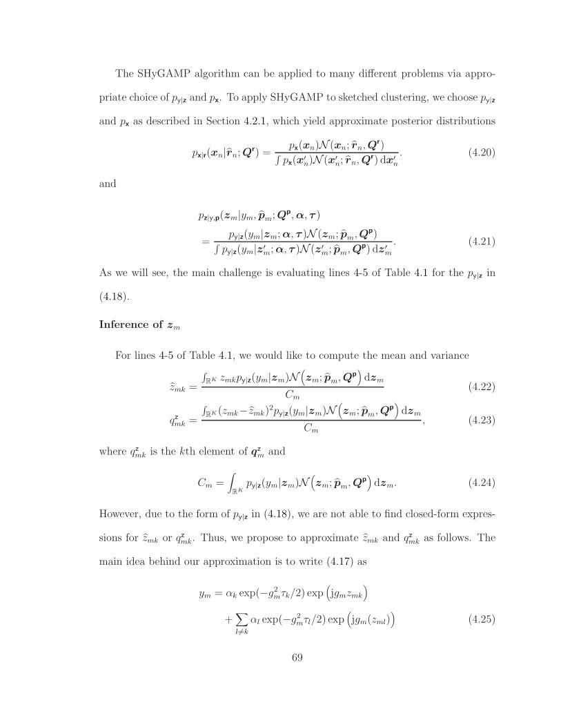
The SHyGAMP algorithm can be applied to many different problems via appro-

priate choice of py|z and px. To apply SHyGAMP to sketched clustering, we choose py|z

and px as described in Section 4.2.1, which yield approximate posterior distributions

px|r(xn|rn; Qr) =px(xn)N (xn; rn, Qr)

∫px(x′

n)N (x′n; rn, Q

r) dx′n

. (4.20)

and

pz|y,p(zm|ym, pm; Qp, α, τ )

=py|z(ym|zm; α, τ )N (zm; pm, Qp)

∫py|z(ym|z′

m; α, τ )N (z′m; pm, Qp) dz′

m

. (4.21)

As we will see, the main challenge is evaluating lines 4-5 of Table 4.1 for the py|z in

(4.18).

Inference of zm

For lines 4-5 of Table 4.1, we would like to compute the mean and variance

zmk =

∫RK zmkpy|z(ym|zm)N

(zm; pm, Qp

)dzm

Cm

(4.22)

qzmk =

∫RK(zmk−zmk)

2py|z(ym|zm)N(zm; pm, Qp

)dzm

Cm, (4.23)

where qzmk is the kth element of qz

m and

Cm =∫

RKpy|z(ym|zm)N

(zm; pm, Qp

)dzm. (4.24)

However, due to the form of py|z in (4.18), we are not able to find closed-form expres-

sions for zmk or qzmk. Thus, we propose to approximate zmk and qz

mk as follows. The

main idea behind our approximation is to write (4.17) as

ym = αk exp(−g2mτk/2) exp

(jgmzmk

)

+∑

l 6=k

αl exp(−g2mτl/2) exp

(jgm(zml)

)(4.25)

69

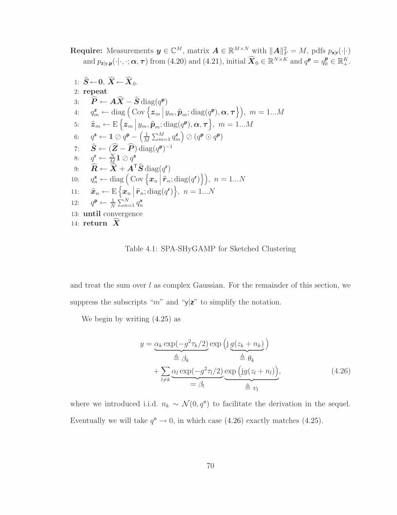
Require: Measurements y ∈ CM , matrix A ∈ R

M×N with ‖A‖2F = M , pdfs px|r(·|·)and pz|y,p(·|·, ·; α, τ ) from (4.20) and (4.21), initial X0 ∈ RN×K and qp = qp

0 ∈ RK+ .

1: S←0, X←X0.2: repeat

3: P ← AX − S diag(qp)

4: qzm ← diag

(Cov

{zm

∣∣∣ ym, pm; diag(qp), α, τ})

, m = 1...M

5: zm ← E{zm

∣∣∣ ym, pm; diag(qp), α, τ}, m = 1...M

6: qs ← 1⊘ qp −(

1M

∑Mm=1 qz

m

)⊘ (qp ⊙ qp)

7: S ← (Z − P ) diag(qp)−1

8: qr ← NM

1⊘ qs

9: R← X + ATS diag(qr)

10: qxn ← diag

(Cov

{xn

∣∣∣ rn; diag(qr)})

, n = 1...N

11: xn ← E{xn

∣∣∣ rn; diag(qr)}, n = 1...N

12: qp ← 1N

∑Nn=1 qx

n

13: until convergence14: return X

Table 4.1: SPA-SHyGAMP for Sketched Clustering

and treat the sum over l as complex Gaussian. For the remainder of this section, we

suppress the subscripts “m” and “y|z” to simplify the notation.

We begin by writing (4.25) as

y = αk exp(−g2τk/2)︸︷︷︸, βk

exp(j g(zk + nk)︸︷︷︸

, θk

)

+∑

l 6=k

αl exp(−g2τl/2)︸︷︷︸= βl

exp(jg(zl + nl)

)

︸︷︷︸, vl

, (4.26)

where we introduced i.i.d. nk ∼ N (0, qn) to facilitate the derivation in the sequel.

Eventually we will take qn → 0, in which case (4.26) exactly matches (4.25).

70

Next we derive an expression for the marginal posterior p(zk|y) under the pseudo-

prior zk ∼ N (pk, qpk) ∀k. First,

p(zk|y) =∫

RKp(z, θk|y) dθk dz\k (4.27)

=1

p(y)

∫

RKp(y|z, θk)p(θk|z)p(z) dθk dz\k (4.28)

=1

p(y)

∫

RKp(y|z\k, θk)N (θk; gzk, g

2qn)

×K∏

l=1

N (zl; pl, qpl ) dθk dz\k, (4.29)

where z\k , [z1, . . . , zk−1, zk+1, . . . , zK ]T. A change-of-variables from zl to zl , zl− pl

for all l 6= k gives

p(zk|y) =N (zk; pk, q

pk)

p(y)

∫

R

N (θk; gzk, g2qn) (4.30)

×∫

RK−1

p(y|z\k, θk)∏

l 6=k

N (zl; 0, qpl ) dz\k

dθk,

where p(y|z\k, θk) is associated with the generative model

y = βk exp(jθk) +∑

l 6=k

βl exp(jg(pl + zl + nl)

)(4.31)

with i.i.d. nl ∼ N (0, qn). Now, because zl and nl are (apriori) mutually independent

zero-mean Gaussian variables, we can work directly with the sum nl , zl + nl ∼

N (0, qpl + qn) and thus bypass the inner integral in (4.30). This allows us to write

p(zk|y) =N (zk; pk, q

pk)

p(y)

∫

R

N (θk; gzk, g2qn)p(y|θk) dθk, (4.32)

where p(y|θk) is associated with the generative model

y = βk exp(jθk) +∑

l 6=k

βl exp(jg(pl + nl))︸︷︷︸= vl

(4.33)

71

with i.i.d. nl ∼ N (0, qpl + qn). Recalling that y ∈ C, it will sometimes be useful to

write (4.33) as

[Re{y}Im{y}

]∼ N

(βk

[cos(θk)sin(θk)

]+∑

l 6=k

βl E

{[Re{vl}Im{vl}

]},

∑

l 6=k

β2l Cov

{[Re{vl}Im{vl}

]}). (4.34)

To compute the posterior mean of zk, (4.32) implies

zk , E{zk|y} =∫

R

zk p(zk|y) dzk (4.35)

=1

p(y)

∫

R

[∫

R

zkN (gzk; θk, g2qn)N (zk; pk, q

pk) dzk

]

× p(y|θk) dθk (4.36)

=∫

R

∫

R

zkN

zk;

θk/gqn + pk

qp

k

1qn + 1

qp

k

,1

1qn + 1

qp

k

dzk

×N(θk; gpk, g

2(qn + qpk))

p(y|θk)

p(y)︸︷︷︸= p(θk|y)

dθk (4.37)

=∫

R

θk/gqn + pk

qpk

1qn + 1

qpk

p(θk|y) dθk (4.38)

=pk

qpk/q

n + 1+

θk/g

1 + qn/qpk

for θk ,∫

R

θk p(θk|y) dθk, (4.39)

where the Gaussian pdf multiplication rule14 was used in (4.37) and where θk denotes

the posterior mean of θk.

14N (x; a, A)N (x; b, B) = N (0; a − b, A + B)N(x; (A−1 + B−1)−1(A−1a + B−1b), (A−1 +

B−1)−1).

72

For the posterior variance of zk, a similar approach gives

qzk , var{zk|y} =

∫

R

(zk − zk

)2p(zk|y) dzk (4.40)

=1

p(y)

∫

R

[ ∫

R

(zk−zk)2N (gzk; θk, g

2qn)

×N (zk; pk, qpk) dzk

]p(y|θk) dθk (4.41)

=∫

R

∫

R

(zk−zk)2N

zk;

θk/gqn + pk

qpk

1qn + 1

qpk

,1

1qn + 1

qpk

dzk

× p(θk|y) dθk. (4.42)

Using a change-of-variables from zk to zk , zk − zk, we get

qzk =

∫

R

∫

R

z2kN

zk;

θk/gqn − θk/g

qn

1qn + 1

qpk

,1

1qn + 1

qpk

dzk

× p(θk|y) dθk (4.43)

=∫

R

(

(θk − θk)/g

1 + qn/qpk

)2

+qn

1 + qn/qpk

p(θk|y) dθk (4.44)

=qn

1+qn/qpk

+1

g2

(1

1+qn/qpk

)2 ∫

R

(θk−θk)2 p(θk|y) dθk

︸︷︷︸, qθ

k = var{θk|y}

. (4.45)

The computation of zk and qzk is still complicated by the form of the posterior

p(θk|y) implied by (4.33). To circumvent this problem, we propose to apply a Gaussian

approximation to the sum in (4.33). Because {nl}∀l 6=k are mutually independent, the

mean and covariance of the sum in (4.33) are simply the sum of the means and

covariances (respectively) of the K − 1 terms making up the sum. Recalling (4.34),

this implies that

p

([Re{y}Im{y}

] ∣∣∣∣∣θk

)≈ N

([Re{y}Im{y}

]; βk

[cos(θk)sin(θk)

]+ µk,Σk

)(4.46)

73

with

µk =∑

l 6=k

αle−g2(τk+qp

k)/2

[cos(gpl)sin(gpl)

](4.47)

Σk =1

2

∑

l 6=k

β2l

(1− e−g2qp

l

)

×(I − e−g2qp

l

[cos(2gpl) sin(2gpl)sin(2gpl) − cos(2gpl)

]). (4.48)

We note that (4.47) and (4.48) were obtained using

E{

Re{vl}}

= exp(− g2qp

l /2)

cos(gpl) (4.49)

E{

Im{vl}}

= exp(− g2qp

l /2)

sin(gpl) (4.50)

2 E{

Re{vl}2}

= 1 + exp(− g2qp

l

)cos(2gpl) (4.51)

2 E{

Im{vl}2}

= 1− exp(− g2qp

l

)cos(2gpl) (4.52)

2 E{

Re{vl} Im{vl}}

= exp(− g2qp

l

)sin(2gpl), (4.53)

which use the fact that, after letting qn → 0,

E{vl} =∫

R

N (zl; pl, qpl ) exp(jgzl) dzl (4.54)

= exp(jgpl − g2qp

l /2). (4.55)

Rewriting (4.46) as

p

(β−1

k

[Re{y}Im{y}

] ∣∣∣∣∣θk

)(4.56)

≈ N([

cos(θk)sin(θk)

]; β−1

k

[Re{y}Im{y}

]− β−1

k µk, β−2k Σk

),

the right side of (4.56) can be recognized as being proportional to the generalized von

Mises (GvM) density over θk ∈ [0, 2π) from [63]. Under this GvM approximation, we

have [63] that

p(y|θk) ∝ exp(κk cos(θk − ζk) + κk cos[2(θk − ζk)]

)(4.57)

74

for parameters κk, κk > 0 and ζk, ζk ∈ [0, 2π) defined from β−1k y, β−1

k µk, and β−2k Σk.

In particular,

κk cos(ζk) = − 1

1− ρ2k

(ρkνk

σkσk

− νk

σ2k

)(4.58)

κk sin(ζk) = − 1

1− ρ2k

(ρkνk

σkσk

− νk

σ2k

)(4.59)

κk cos(2ζk) = − 1

4(1− ρ2k)

(1

σ2k

− 1

σ2k

)(4.60)

κk sin(2ζk) =ρk

2(1− ρ2k)σkσk

, (4.61)

where

[νk

νk

], β−1

k

([Re{y}Im{y}

]− µk

)(4.62)

[σ2

k ρkσkσk

ρkσkσk σ2k

], β−2

k Σk. (4.63)

From (4.57) and the SHyGAMP pseudo-prior zk ∼ N (pk, qpk), we see that the posterior

on θk takes the form

p(θk|y) ∝ N(θk; gpk, g

2qpk

)p(y|θk) (4.64)

∝ exp

[κk cos(θk − ζk) + κk cos[2(θk − ζk)]−

(θk − gpk)2

2g2qpk

]. (4.65)

We now face the task of computing θk = E{θk|y} and qθk = var{θk|y} under

(4.65). Since these quantities do not appear to be computable in closed form,

we settle for an approximation, such as that based on the Laplace approxima-

tion [23] or numerical integration. For the Laplace approximation, we would first

compute θk,MAP , arg maxθkln p(θk|y) and then approximate θk ≈ θk,MAP and

qθk ≈ − d2

dθk2 ln p(θk|y)

∣∣∣θk=θk,MAP

. However, since computing arg maxθkln p(θk|y) is com-

plicated due to the presence of multiple local maxima, we instead use numerical inte-

gration. For this, we suggest a grid of NptsNper + 1 uniformly-spaced points centered

75

at gpk with width 2πNper, where Nper =⌈

Nstd

π

√g2qp

k

⌉. This choice of grid ensures

that the sampling points cover at least Nstd standard deviations of the prior on θk.

We used Nstd = 4 and Npts = 7 in the numerical experiments in Section 4.3.

Finally, after approximating θk and qθk via numerical integration, we set zk = θk/g

and qzk = qθ

k/g2.

Inference of xn

Recall that lines 10-11 of Table 4.1 support an arbitrary prior px on xn. For the

experiments in Section 4.3, we used the trivial non-informative prior px(xn) ∝ 1, after

which lines 10-11 reduce to

qxn = qr ∀n and xn = rn ∀n. (4.66)

4.2.4 Initialization

We recommend initializing CL-AMP with X = X0 and qp = qp0 , where X0

is drawn i.i.d. N (0, σ2) and where qp0 = σ21, with σ2 from (4.79) (as described in

Section 4.2.7).

In some cases, running CL-AMP from R > 1 different random initializations can

help avoid to spurious solutions. Here, CL-AMP is run from a different random

initialization X0,r, for r = 1, . . . , R, and then the quality of the recovered solution

Xr is evaluated by constructing the “estimated sketch” yr via

ymr =K∑

k=1

αk exp(−g2mτk) exp(jgmaT

mxkr) (4.67)

recalling (4.9) and (4.17), and then measuring its distance to the true sketch y. The

initialization index is then selected as

r∗ = arg minr‖y − yr‖, (4.68)

76

and the centroids saved as X = Xr∗ . In Section 4.3, we used R = 2 for all experi-

ments.

4.2.5 Hyperparameter Tuning

The likelihood model py|z in (4.18) depends on the unknown hyperparameters

α and τ . We propose to estimate these hyperparameters using a combination of

expectation maximization (EM) and SHyGAMP, as suggested in [9] and detailed—for

the simpler case of GAMP—in [4]. The idea is to run SHyGAMP using an estimate of

α and τ , update α and τ from the SHyGAMP outputs, and repeat until convergence.

For the first estimate, we suggest to use αk = 1K

and τk = 0 ∀ k.

Extrapolating [4, eq. (23)] to the SHyGAMP case, the EM update of (α, τ ) takes

the form

(α, τ ) = arg maxα≥0,αT1=1,τ>0

M∑

m=1

∫

RKN (zm; zm, Qz

m) (4.69)

× ln py|z(ym|zm; α, τ ) dzm,

where zm and Qzm = diag{qz

m} are obtained by running SHyGAMP to convergence

under (α, τ ). To proceed, we model the Dirac delta in (4.18) using a circular Gaussian

pdf with vanishingly small variance ǫ > 0, in which case

ln py|z(ym|zm; α, τ ) (4.70)

= −1

ǫ

∣∣∣∣∣ym −K∑

k=1

αk exp

(jgmzmk −

g2mτk

2

)∣∣∣∣∣

2

+ const.

77

Plugging (4.70) back into (4.69), we see that the constant and the 1/ǫ-scaling play

no role in the optimization, and so we can discard them to obtain

(α, τ ) = arg minα≥0,αT1=1,τ>0

M∑

m=1

∫

RKN (zm; zm, Qz

m) (4.71)

×∣∣∣∣∣ym −

K∑

k=1

αk exp

(jgmzmk −

g2mτk

2

)∣∣∣∣∣

2

dzm.

A closed-form solution to the optimization problem in (4.71) seems out of reach.

Also, the optimization objective is convex in α for fixed τ , and convex in τ for fixed

α, but not jointly convex in [αT, τT]. Although the optimization problem (4.71) is

difficult to solve, the solutions obtained by gradient projection (GP) [43] seem to work

well in practice. Also, GP is made practical by closed-form gradient expressions. In

particular, let

qmk , exp

(− g2

mτk

2

)(4.72)

ρmk , exp

(jgmzmk−

qzmkg

2m

2

), (4.73)

and recall that vmk = exp(jgmzmk) from (4.26). Then the mth term of the sum in the

objective in (4.71) becomes

∫

RKN (zm; zm, Qz

m)

∣∣∣∣∣ym −K∑

k=1

αkqmkvmk

∣∣∣∣∣

2

dzm

= |ym|2 − 2K∑

k=1

αkqmk Re{y∗

mρmk

}

+K∑

k=1

αkqmkρ∗mk

K∑

l 6=k

αlqmlρml +K∑

k=1

α2kq

2mk, (4.74)

78

where we used the fact that∫RN (zmk; zmk, q

zmk)vmk dzmk = ρmk. After reapplying the

sum over m, we get

∂

∂αk

M∑

m=1

∫

RKN (zm; zm, Qz

m)

∣∣∣∣∣ym−K∑

k=1

αkqmkvmk

∣∣∣∣∣

2

dzm

= −2M∑

m=1

qmkγmk (4.75)

∂

∂τk

M∑

m=1

∫

RKN (zm; zm, Qz

m)

∣∣∣∣∣ym−K∑

k=1

αkqmkvmk

∣∣∣∣∣

2

dzm

= αk

M∑

m=1

g2mqmkγmk (4.76)

for

γmk , Re{y∗

mρmk

}− αkqmk −

K∑

l 6=k

αlqml Re{ρ∗

mkρml

}. (4.77)

We found that complexity of hyperparameter tuning can be substantially reduced,

without much loss in accuracy, by using only a subset of the terms in the sum in (4.71),

as well as in the corresponding gradient expressions (4.75)-(4.76). For the experiments

in Section 4.3, we used a fixed random subset of min(M, 20K) terms.

4.2.6 Algorithm Summary

Table 4.2 summarizes the CL-AMP algorithm with R random initializations and

tuning of the hyperparameters (α, τ ). Note that the random initializations {X0,r}

are used only for the first EM iteration, i.e., i = 0. Subsequent EM iterations (i.e.,

i ≥ 1) are initialized using the output X i of the previous EM iteration.

79

Require: Measurements y ∈ CM , gains {gm}Mm=1, number of initializations R ≥ 1, initializations

{X0,r}Rr=1, qp0 , α0, τ 0.

1: i = 02: repeat

3: if i = 0 then

4: for r = 1 : R do

5: Run CL-AMP with fixed (α0, τ 0) from initialization (X0,r, qp0), yielding output X1,r,

Zr, and {qzmr}Mm=1.

6: end for

7: Compute ymr ,∑K

k=1 α0k exp(−g2mτ0k) exp(jgmzmkr) ∀mr

8: Find r∗ = argminr ‖y − yr‖.9: Set X1 = X1,r∗

, Z = Zr∗and {qz

m}Mm=1 = {qzmr∗

}Mm=1.10: else

11: Run CL-AMP with fixed (αi, τ i) from initialization (X i, qp0), yielding output Xi+1, Z,

and {qzm}Mm=1.

12: end if

13: Compute (αi+1, τ i+1) via (4.71) using Z and {qzm}Mm=1.

14: i← i + 1.15: until convergence

Table 4.2: CL-AMP with hyperparameter tuning and multiple random initializations

4.2.7 Frequency Generation

As proposed in [55], am were drawn uniformly on the unit sphere and {gm} were

drawn i.i.d. from the distribution

p(g; σ2) ∝ 1[0,∞)(g)

√

g2σ2 +g4σ4

4exp

(− 1

2g2σ2

), (4.78)

which has parameter σ2. The authors in [55] suggest using σ2 = 1NK

∑Kk=1 tr(Φk)

and propose a method to estimate σ2 from y. However, our numerical experiments

suggest that using

σ2 = E{‖d‖22}/N ≈ ‖D‖2F/NT (4.79)

provides significantly improved performance. Note that the right side of (4.79) can

be computed in an online manner, or approximated using a subset of the data. For

80

the experiments in Section 4.3, we computed σ2 via the right side of (4.79) and used

it in computing qx0 = σ21.

4.3 Numerical Experiments

In this section, we present the results of several experiments used to test the per-

formance of the CL-AMP, CL-OMPR, and k-means++ algorithms. For k-means++,

we used the implementation provided by MATLAB and, for CL-OMPR, we down-

loaded the MATLAB implementation from [64]. CL-OMPR and CL-AMP used the

same sketch y, whose frequency vectors W were drawn using the method described

in Section 4.2.7, with the scaling parameter σ2 set via (4.79). For CL-OMPR and

CL-AMP, the reported runtimes include the time of computing the sketch, unless

otherwise noted. All experiments were run on a Dell PowerEdge C6320 two-socket

server with Intel Xeon E5-2680 v4 processors (14 cores, 2.40GHz) and 128GB RAM.

4.3.1 Experiments with Synthetic Data

Performance vs. sketch length M

In the first experiment, we test each algorithm’s ability to minimize SSE on a set

of training data, i.e., to solve the problem (4.1). In addition, we test how well the

recovered centroids work in minimum-distance classification.

The experiment was conducted as follows. Fixing the number of classes at K = 10

and the data dimension at N = 100, 10 Monte Carlo trials were performed. In each

trial, the true centroids were randomly drawn15 as xk ∼ N (0N , 1.52K2/NIN). Then,

using these centroids, a training dataset {dt}Tt=1 with T = 107 samples was drawn from

15This data-generation model was chosen to match that from [55], and is intended to have arelatively constant Bayes error rate w.r.t. N and K.

81

the GMM (4.5) with weights αk = 1/K and covariances Φk = IN∀k. Additionally, a

test dataset {dt} of 106 samples was independently generated.

For centroid recovery, k-means++ was invoked on the training dataset, and both

CL-AMP and CL-OMPR were invoked after sketching the training data with M

samples as in (4.2). Sketch lengths M/KN ∈ {1, 2, 3, 5, 10, 20} were investigated.

CL-AMP used two random initializations, i.e., R = 2 as defined in Table 4.2.

For each algorithm, the SSE of its estimated centroids {xk}Kk=1 was calculated us-

ing the training data {dt}Tt=1 via (4.1). Additionally, the performance of the estimated

centroids in minimum-distance classification was evaluated as follows. First, labels

{jk}Kk=1 were assigned to the estimated centroids by solving the linear assignment

problem [65] without replacement, given by

arg min{j1,...,jK}={1,...,K}

K∑

k=1

‖xk − xjk‖22. (4.80)

Next, each test sample dt was classified using minimum-distance classification, pro-

ducing the estimated label

kt = arg mink∈{1,...,K}

‖dt − xjk‖. (4.81)

The classification error rate (CER) was then calculated as the proportion of estimated

labels kt that do not equal the true label kt from which the test sample dt was

generated.16

Figures 4.1, 4.2, and 4.3 show the median SSE, CER, and runtime (including

sketching), respectively, for CL-AMP and CL-OMPR versus M/KN . Also shown is

the median SSE, CER, and runtime of k-means++, as a baseline, where k-means++

16Note that the true label kt was assigned when the test sample dt was generated. The true labelkt does not necessarily indicate which of the true centroids {xk} is closest to dt.

82

has no dependence on M . Because a low runtime is meaningless if the corresponding

SSE is very high, the runtime was not shown for CL-AMP and CL-OMPR whenever

its SSE was more than 1.5 times that of k-means++. The error bars show the standard

deviation of the estimates.

10 0 10 10

50

100

150

200

250

300

350

400

CL-AMPCL-OMPRK-means

Med

ian

SSE

M/KN

Figure 4.1: SSE vs. sketch length M for K = 10 clusters, dimension N = 100, andT = 107 training samples.

Figure 4.1 shows that CL-AMP achieved a low SSE with smaller sketch size M

than CL-OMPR. In particular, CL-AMP required M ≈ 2KN to yield a low SSE,

while CL-OMPR required M ≈ 10KN . Also, with sufficiently large M , the SSE

achieved by CL-AMP and CL-OMPR was lower than that achieved by k-means++.

Figure 4.2 shows that CL-AMP achieved a low CER with sketch size M ≈ KN ,

while CL-OMPR required M ≈ 10KN . Also, with sufficiently large M , CL-AMP

83

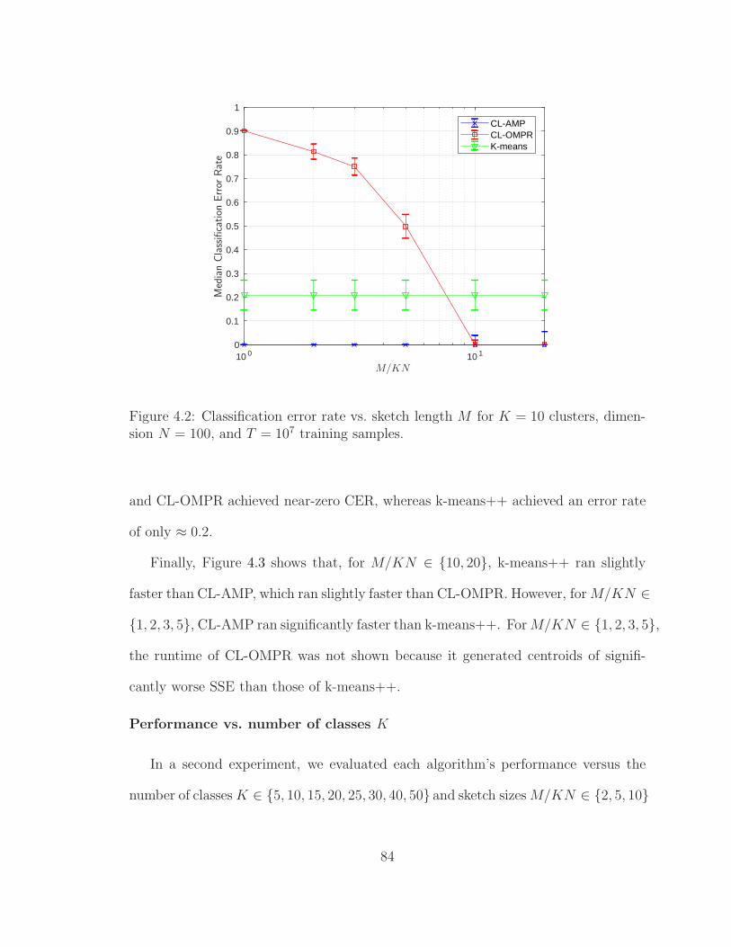
10 0 10 10

0.1

0.2

0.3

0.4

0.5

0.6

0.7

0.8

0.9

1


Med

ian

Cla

ssifi

cation

Err

orRat

e

M/KN

Figure 4.2: Classification error rate vs. sketch length M for K = 10 clusters, dimen-sion N = 100, and T = 107 training samples.

and CL-OMPR achieved near-zero CER, whereas k-means++ achieved an error rate

of only ≈ 0.2.

Finally, Figure 4.3 shows that, for M/KN ∈ {10, 20}, k-means++ ran slightly

faster than CL-AMP, which ran slightly faster than CL-OMPR. However, for M/KN ∈

{1, 2, 3, 5}, CL-AMP ran significantly faster than k-means++. For M/KN ∈ {1, 2, 3, 5},

the runtime of CL-OMPR was not shown because it generated centroids of signifi-

cantly worse SSE than those of k-means++.

Performance vs. number of classes K

In a second experiment, we evaluated each algorithm’s performance versus the

number of classes K ∈ {5, 10, 15, 20, 25, 30, 40, 50} and sketch sizes M/KN ∈ {2, 5, 10}

84

10 0 10 1

100

150

200

250

300

350

400450500550600


Med

ian

Runtim

e(incl

udin

gsk

etch

ing)

M/KN

Figure 4.3: Runtime (including sketching) vs. sketch length M for K = 10 clusters,dimension N = 100, and T = 107 training samples.

for fixed data dimension N = 50. The data was generated in exactly the same way

as the previous experiment, and the same performance metrics were evaluated. Fig-

ures 4.4, 4.5, and 4.6 show the median SSE, CER, and runtime (including sketching),

respectively, versus K, for CL-AMP, CL-OMPR, and k-means++.

Figure 4.4 shows that, as K increases, the SSE of k-means++ remained roughly

constant, as expected based on the generation of the true centers xk. For K ≤ 20,

CL-AMP yielded the best SSE for all tested values of M . For K > 20, CL-AMP

yielded the best SSE with sketch sizes M ∈ {5KN, 10KN}, but performed poorly

with M = 2KN . Meanwhile, CL-OMPR performed reasonably well with sketch size

M = 10KN , but poorly with M ∈ {2KN, 5KN}.

85

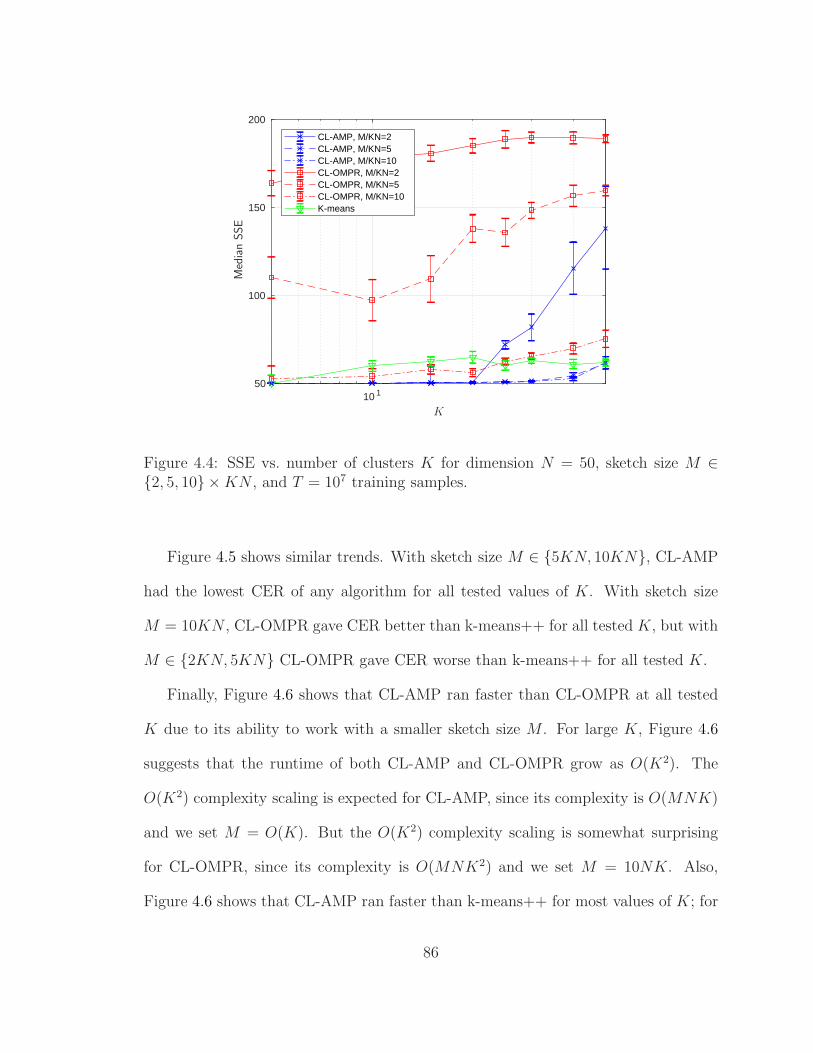
10 150

100

150

200

CL-AMP, M/KN=2CL-AMP, M/KN=5CL-AMP, M/KN=10CL-OMPR, M/KN=2CL-OMPR, M/KN=5CL-OMPR, M/KN=10K-means

Med

ian

SSE

K

Figure 4.4: SSE vs. number of clusters K for dimension N = 50, sketch size M ∈{2, 5, 10} ×KN , and T = 107 training samples.

Figure 4.5 shows similar trends. With sketch size M ∈ {5KN, 10KN}, CL-AMP

had the lowest CER of any algorithm for all tested values of K. With sketch size

M = 10KN , CL-OMPR gave CER better than k-means++ for all tested K, but with

M ∈ {2KN, 5KN} CL-OMPR gave CER worse than k-means++ for all tested K.

Finally, Figure 4.6 shows that CL-AMP ran faster than CL-OMPR at all tested

K due to its ability to work with a smaller sketch size M . For large K, Figure 4.6

suggests that the runtime of both CL-AMP and CL-OMPR grow as O(K2). The

O(K2) complexity scaling is expected for CL-AMP, since its complexity is O(MNK)

and we set M = O(K). But the O(K2) complexity scaling is somewhat surprising

for CL-OMPR, since its complexity is O(MNK2) and we set M = 10NK. Also,

Figure 4.6 shows that CL-AMP ran faster than k-means++ for most values of K; for

86

10 1-0.2

0

0.2

0.4

0.6

0.8

1


Med

ian

Cla

ssifi

cation

Err

orRat

e

K

Figure 4.5: Classification Error Rate vs. number of clusters K for dimension N = 50,sketch size M ∈ {2, 5, 10} ×KN , and T = 107 training samples.

the smallest tested value of K (i.e., K = 5), the median runtime of k-means++ was

lower than CL-AMP (but the error-bar suggests that the runtime of k-means++ was

highly variable at this K). For the largest tested value of K, k-means++ was again

faster than CL-AMP, because the runtime of k-means++ is expected to grow linearly

with K, whereas that of CL-AMP is expected to grow quadratically with K when

M/KN is fixed.

Performance vs. dimension N

In a third experiment, we evaluated each algorithm’s performance versus the di-

mension N (logarithmically spaced between 10 and 316) for K = 10 classes and sketch

size M ∈ {2, 5, 10} ×KN . The data was generated in exactly the same way as the

87

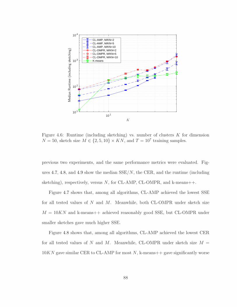
10 110 1

10 2

10 3

10 4


Med

ian

Runtim

e(incl

udin

gsk

etch

ing)

K

Figure 4.6: Runtime (including sketching) vs. number of clusters K for dimensionN = 50, sketch size M ∈ {2, 5, 10} ×KN , and T = 107 training samples.

previous two experiments, and the same performance metrics were evaluated. Fig-

ures 4.7, 4.8, and 4.9 show the median SSE/N , the CER, and the runtime (including

sketching), respectively, versus N , for CL-AMP, CL-OMPR, and k-means++.

Figure 4.7 shows that, among all algorithms, CL-AMP achieved the lowest SSE

for all tested values of N and M . Meanwhile, both CL-OMPR under sketch size

M = 10KN and k-means++ achieved reasonably good SSE, but CL-OMPR under

smaller sketches gave much higher SSE.

Figure 4.8 shows that, among all algorithms, CL-AMP achieved the lowest CER

for all tested values of N and M . Meanwhile, CL-OMPR under sketch size M =

10KN gave similar CER to CL-AMP for most N , k-means++ gave significantly worse

88

CER compared to CL-AMP for all N , and CL-OMPR under sketch size M = 5KN

or 2KN gave even worse CER for all N .

Finally, Figure 4.9 shows that, among all algorithms, CL-AMP with sketch size

M = 2KN ran the fastest for all tested values of N . Meanwhile, CL-OMPR with

sketch size M = 10KN ran at a similar speed to CL-AMP with sketch size M =

10KN , for all N . The runtimes for CL-OMPR with smaller sketches are not shown

because it achieved significantly worse SSE than k-means++. Figure 4.9 suggests

that, if N is increased beyond 316, then eventually k-means++ will be faster than

CL-AMP under fixed M/KN .

10 1 10 20.5

1

1.5

2

2.5

3

3.5

4


Med

ian

SSE/N

N

Figure 4.7: SSE/N vs. dimension N for K = 10 classes, T = 107 samples, and sketchsize M ∈ {2, 5, 10} ×KN .

89

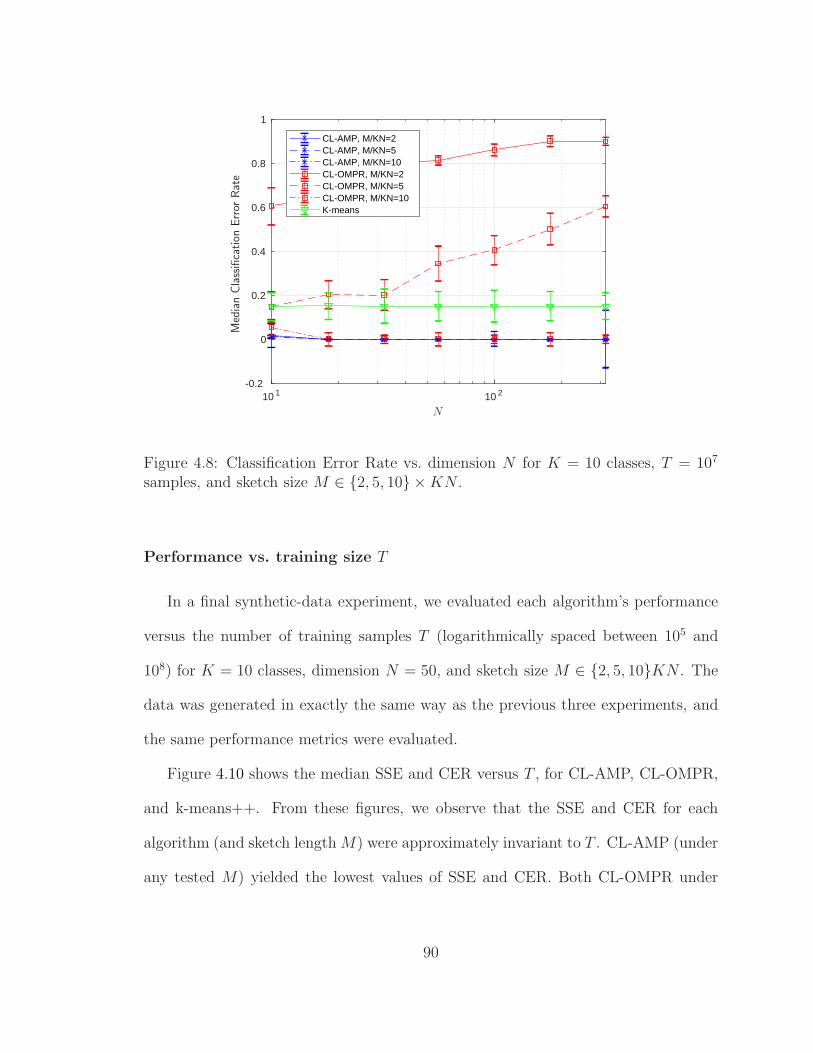
10 1 10 2-0.2

0

0.2

0.4

0.6

0.8

1


Med

ian

Cla

ssifi

cation

Err

orRat

e

N

Figure 4.8: Classification Error Rate vs. dimension N for K = 10 classes, T = 107

samples, and sketch size M ∈ {2, 5, 10} ×KN .

Performance vs. training size T

In a final synthetic-data experiment, we evaluated each algorithm’s performance

versus the number of training samples T (logarithmically spaced between 105 and

108) for K = 10 classes, dimension N = 50, and sketch size M ∈ {2, 5, 10}KN . The

data was generated in exactly the same way as the previous three experiments, and

the same performance metrics were evaluated.

Figure 4.10 shows the median SSE and CER versus T , for CL-AMP, CL-OMPR,

and k-means++. From these figures, we observe that the SSE and CER for each

algorithm (and sketch length M) were approximately invariant to T . CL-AMP (under

any tested M) yielded the lowest values of SSE and CER. Both CL-OMPR under

90

10 1 10 210 1

10 2

10 3

10 4


Med

ian

Runtim

e(incl

udin

gsk

etch

ing)

N

Figure 4.9: Runtime (including sketching) vs. dimension N for K = 10 classes, T =107 samples, and sketch size M ∈ {2, 5, 10} ×KN .

sketch size M = 10KN and k-means++ gave reasonably good SSE and CER, but

CL-OMPR under smaller sketches gave worse SSE and CER.

Then, Figure 4.11 shows the median runtime with and without sketching, respec-

tively, for the algorithms under test. Figure 4.11a shows that, if sketching time is

included in runtime, then all runtimes increased linearly with training size T . How-

ever, for large T , CL-AMP ran faster than k-means++ and CL-OMPR (while also

achieving lower SSE and CER). Meanwhile, Figure 4.11b shows that, if sketching time

is not included in runtime, then the runtimes of both CL-AMP and CL-OMPR were

relatively invariant to T . Also, Figure 4.11 shows that, for T > 106, the sketching

time was the dominant contributer to the overall runtime.

91

10 5 10 6 10 7 10 840

60

80

100

120

140

160

180

200


Med

ian

SSE

T

(a) SSE vs. T

10 5 10 6 10 7 10 8-0.1

0

0.1

0.2

0.3

0.4

0.5

0.6

0.7

0.8

0.9


Med

ian

Cla

ssifi

cation

Err

orRat

e

T

(b) Classification Error Rate vs. T

Figure 4.10: Performance vs. training size T for K = 10 classes, dimension N = 50,and sketch size M ∈ {2, 5, 10} ×KN .

92

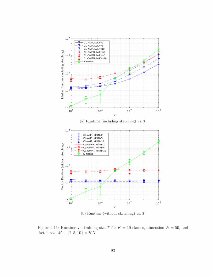
10 5 10 6 10 7 10 810 0

10 1

10 2

10 3

10 4


Med

ian

Runtim

e(incl

udin

gsk

etch

ing)

T

(a) Runtime (including sketching) vs. T

10 5 10 6 10 7 10 810 0

10 1

10 2

10 3

10 4


Med

ian

Runtim

e(w

ithou

tsk

etch

ing)

T

(b) Runtime (without sketching) vs. T

Figure 4.11: Runtime vs. training size T for K = 10 classes, dimension N = 50, andsketch size M ∈ {2, 5, 10} ×KN .

93

4.3.2 Spectral Clustering of MNIST

Next we evaluated the algorithms on the task of spectral clustering [66] of the

MNIST dataset. This task was previously investigated for CL-OMPR and k-means++

in [56], and we used the same data preprocessing steps: extract SIFT descriptors [67]

of each image, compute the K-nearest-neighbors adjacency matrix (for K = 10) using

FLANN [68], and compute the 10 principal eigenvectors of the associated normalized

Laplacian matrix (since we know K = 10), yielding features of dimension N = 10.

We applied this process to the original MNIST dataset, which includes T = 7× 104

samples, as well as an augmented one with T = 3 × 105 samples constructed as

described in [56].

The experiment was conducted as follows. In each of 10 trials, we randomly

partitioned each sub-dataset into equally-sized training and testing portions. Then,

we invoked CL-AMP, CL-OMPR, and k-means++ on the training portion of the

dataset, using sketch sizes M ∈ {1, 2, 3, 5, 10} × KN for CL-AMP and CL-OMPR.

The algorithm parameters were the same as in Section 4.3.1. Finally, the estimated

centroids produced by each algorithm were evaluated using the same two metrics as

in Section 4.3.1: SSE on the training data, and classification error rate (CER) when

the centroids were used for minimum-distance classification of the test data samples.

The median SSE, CER, and runtime, versus sketch length M , are shown for CL-

AMP and CL-OMPR in Figures 4.12-4.14, respectively, for the T = 7 × 104-sample

MNIST sub-dataset, and in Figures 4.15-4.17, respectively, for T = 3 × 105-sample

MNIST sub-dataset. As before, k-means++ is shown, as a baseline, although it

does not use the sketch and thus is performance is invariant to M . From these

figures, we observe that CL-AMP and CL-OMPR gave respectable results for sketch

94

lengths M ≥ 2KN , and SSE nearly identical to kmeans++ for M ≥ 5KN . For

M ≥ 2KN , however, CL-AMP yielded significantly lower CER than both CL-OMPR

and k-means++, at the cost of a slower runtime. We attribute CL-AMP’s slower

runtime to its use of many iterations i in Table 4.2 for hyperparameter tuning.

1 2 3 4 5 6 7 8 9 10-0.1

0

0.1

0.2

0.3

0.4

0.5

0.6

0.7

0.8


M/KN

Med

ian

SSE

Figure 4.12: SSE vs. M for the T = 70 000-sample spectral MNIST dataset, withK = 10 clusters and dimension N = 10.

4.3.3 Frequency Estimation

Our final experiment concerns multi-dimensional frequency estimation. Consider

a sum-of-sinusoids signal of the form

y(t) =K∑

k=1

αk exp(jtTxk), (4.82)

95

1 2 3 4 5 6 7 8 9 10-0.1

0

0.1

0.2

0.3

0.4

0.5

0.6

0.7


M/KN

Med

ian

Cla

ssifi

cation

Err

orRat

e

Figure 4.13: Classification Error Rate vs. M for the T = 70 000-sample spectralMNIST dataset, with K = 10 clusters and dimension N = 10.

where xk ∈ RN is the frequency of the kth sinusoid, αk > 0 is the amplitude of the

kth sinusoid, and t ∈ RN denotes time. Given measurements of the signal y(t) at a

collection of random times t ∈ {tm}Mm=1, i.e.,

ym = y(tm) for m = 1, . . . , M, (4.83)

we seek to recover the frequencies {xk}Kk=1. We are particularly interested in the case

where the frequencies {xk} are closely spaced, i.e., the “super-resolution” problem.

Note that the model in (4.82) matches that in (4.13) with gmam = tm ∀m and

Φk = 0∀k, so that we can apply CL-AMP to this frequency estimation problem. The

model in (4.82) also matches (4.4) with wm = tm ∀m, and so we can also apply

CL-OMPR. But we cannot apply k-means++.

96

1 2 3 4 5 6 7 8 9 100

2

4

6

8

10

12

14

16

18


M/KN

Med

ian

Runtim

e(incl

udin

gsk

etch

ing)

Figure 4.14: Runtime (including sketching) vs. M for the T = 70 000-sample spectralMNIST dataset, with K = 10 clusters and dimension N = 10.

For frequency pairs {x1, x2} with ‖x1 − x2‖2 ≥ ǫ, [69] claims that, with {wm}

drawn randomly from an appropriate distribution, one can resolve the frequencies

with M ≥ O(

ln(1/ǫ))

measurements. However, choosing wm uniformly spaced on a

grid would require M ≥ O(1/ǫ) measurements. Thus, for a final experiment, similar

to those performed in [69], we did the following. For a particular N and K (where

K is even for simplicity), we generated K/2 pairs of frequencies {x2k−1, x2k}, where

‖x2k−1 − x2k‖2 = ǫ for k = 1, ..., K/2. Then, for a particular realization of {xk}Kk=1

and {wm}Mm=1, CL-AMP and CL-OMPR were invoked to estimate {xk}Kk=1. Recovery

was declared successful if

maxk‖xjk

− xk‖2 < ǫ/2, (4.84)

where {jk}Kk=1 solves the linear assignment problem (4.80).

97

1 2 3 4 5 6 7 8 9 10-0.1

0

0.1

0.2

0.3

0.4

0.5

0.6

0.7

0.8


M/KN

Med

ian

SSE

Figure 4.15: SSE vs. M for the T = 300 000-sample spectral MNIST dataset, withK = 10 clusters and dimension N = 10.

For our experiment, we tested K = 4 frequency components of dimension N = 2

and varied M from 3KN to 100KN while also varying ǫ from 10−1 to 10−3. For

each combination, 10 trials were performed. The empirical probability of successful

recovery is shown in Figures 4.18-4.19. In Figure 4.18, am were drawn uniformly on

the unit sphere and gm = |g′m| with g′

m ∼ N(0, 4ǫ2 log2

10(ǫ)). Superimposed on the

figures are curves showing M/KN = 0.1/ǫ and M/KN = ln(1/ǫ). From the figures,

we see that CL-AMP had a higher empirical probability of recovery than CL-OMPR,

especially for small ǫ. We also see that the empirical phase transition of CL-AMP is

close to the ln(1/ǫ) curve with random frequency samples and the 0.1/ǫ curve with

uniform frequency samples.

98

1 2 3 4 5 6 7 8 9 10-0.1

0

0.1

0.2

0.3

0.4

0.5

0.6

0.7

0.8


M/KN

Med

ian

Cla

ssifi

cation

Err

orRat

e

Figure 4.16: Classification Error Rate vs. M for the T = 300 000-sample spectralMNIST dataset, with K = 10 clusters and dimension N = 10.

4.4 Conclusion

In sketched clustering, the original dataset is sketched down to a relatively short

vector, from which the centroids are extracted. For the sketch proposed by [55, 56],

we proposed the “CL-AMP” centroid-extraction method. Our method assumes that

the original data follows a GMM, and exploits the recently proposed simplified hy-

brid generalized approximate message passing (SHyGAMP) algorithm [9]. Numerical

experiments suggest that CL-AMP exhibits better sample complexity (i.e., extracts

accurate clusters with fewer compressed samples) than the state-of-the-art sketched-

clustering algorithm, CL-OMPR, from [55,56]. In many cases, CL-AMP also exhibits

better computational complexity than CL-OMPR. Furthermore, for datasets with

99

1 2 3 4 5 6 7 8 9 100

2

4

6

8

10

12

14

16

18

20


M/KN

Med

ian

Runtim

e(incl

udin

gsk

etch

ing)

Figure 4.17: Runtime (including sketching) vs. M for the T = 300 000-sample spectralMNIST dataset, with K = 10 clusters and dimension N = 10.

many samples, CL-AMP exhibits lower computational complexity than the widely

used k-means++ algorithm. As future work, it would be interesting to consider the

use of fast deterministic sketching with CL-AMP.

100

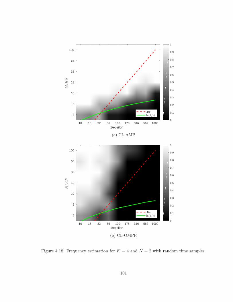
10 18 32 56 100 178 316 562 1000

1/epsilon

100

56

32

18

10

6

3

0

0.1

0.2

0.3

0.4

0.5

0.6

0.7

0.8

0.9

1

.1/e

M/K

N

ln(1/ǫ)

(a) CL-AMP

10 18 32 56 100 178 316 562 1000

1/epsilon

100

56

32

18

10

6

3

0

0.1

0.2

0.3

0.4

0.5

0.6

0.7

0.8

0.9

1

.1/e

M/K

N

ln(1/ǫ)

(b) CL-OMPR

Figure 4.18: Frequency estimation for K = 4 and N = 2 with random time samples.

101

10 18 32 56 100 178 316 562 1000

1/epsilon

100

56

32

18

10

6

3

0

0.1

0.2

0.3

0.4

0.5

0.6

0.7

0.8

0.9

1

.1/e

M/K

N

ln(1/ǫ)

(a) CL-AMP

10 18 32 56 100 178 316 562 1000

1/epsilon

100

56

32

18

10

6

3

0

0.1

0.2

0.3

0.4

0.5

0.6

0.7

0.8

0.9

1

.1/e

M/K

N

ln(1/ǫ)

(b) CL-OMPR

Figure 4.19: Frequency estimation for K = 4 and N = 2 with uniformly spaced timesamples.

102

Chapter 5: Adaptive Detection from Quantized

Measurements

5.1 Introduction and Motivation

In this final chapter, we consider the problem of adaptive detection from highly

quantized measurements, specifically in the case of strong, but low-rank interference.

The motivation for studying this problem is the following. In military communications

the receiver may experience strong jamming from a few number of sources and in

order to effectively null the interference, a large number of antennas at the receiver are

required. However, using more antennas increases the hardware complexity due to the

increased number of analog to digital converters (ADCs) and related components, as

well as increasing the total amount of data that must be processed. For this reason, it

may be desirable to use few-bit or even 1-bit ADCs, which may decrease the amount

of data to be processed, as well as simplify hardware design at the antenna (1-bit

ADCs in particular greatly decrease the hardware complexity at the receiver).

However, using low-resolution ADCs introduces new challenges. In particular,

quantization introduces error in the measurements, and it may affect how one chooses

to process the data. Existing algorithms for signal detection assume unquantized

measurements, and it is unclear how they will perform when applied to quantized data.

103

In this chapter, we first apply unquantized detection algorithms to quantized data to

study how well this approach works. We observe that the primary regime of failure

is when the interference power is too large. We then investigate various alternatives

to how we process the data in order to have improved detection performance at large

interference levels. The various approaches we consider are:

1. standard methods for improving the performance of quantized systems, such as

dithering and companding,

2. alternate detection statistics computed using the generalized likelihood ratio

test (GLRT) and the true quantization model, and

3. various analog pre-processing techniques to remove interference prior to quan-

tization.

The primary connection between this chapter and the rest of this dissertation is in

item 2 above. In particular, we see that the GLRT that uses the true quantization

model involves generalized bilinear inference (see Section 1.1.3), for which approxi-

mate message passing and other techniques exist.

5.1.1 Problem Statement

Our objective is to determine the presence or absence of a known signal s, where

the system model under the H1 and H0 hypotheses is

H1 : Y = QB,∆

(hsH + GΨH + W

)(5.1a)

H0 : Y = QB,∆

(GΨH + W

), (5.1b)

where Y ∈ Cnr×ns are the quantized measurements, h ∈ Cnr is the unknown array

response of the signal, s ∈ Cns is the signal, G ∈ Cnr×ni is the unknown array response

104

of the interference, Ψ ∈ Cns×ni is the unknown interference, and W is circular AWGN

with variance σ2w. The low-rank interference is intended to model a few number of

interference sources whose array responses are time invariant. We assume ns ≥ nr,

in which case our model can also generalize to the case of full rank interference by

assuming G and Ψ both have rank nr.

For x ∈ C, QB,∆(x) , QB,∆(Re(x)) + jQB,∆(Im(x)), where

QB,∆(x ∈ R) ,

max

min

{∆(⌈

x∆

⌉− 1/2

), ∆c

},−∆c

if B ≥ 2

sgn(x) if B = 1

, (5.2)

where ∆c = ∆(2B−1 − 1/2). For B ≥ 2, (5.2) is the element-wise, B-bit, mid-rise,

uniform quantization function with bin size ∆.

5.1.2 Unquantized Detectors

The GLRT for the unquantized model, given by

H1 : U = hsH + GΨH + W (5.3a)

H0 : U = GΨH + W , (5.3b)

has been studied in depth for various assumptions on the various parameters.

Kelly [70,71] treated GΨH +W as temporally white and Gaussian with unknown

spatial covariance matrix Σ > 0. In this case, the GLRT is

maxh,Σ p(U |H1; h,Σ)

maxΣ p(U |H0;Σ)

H1

RH0

τ, (5.4)

which reduces to∏nr

n=1 λ0,n∏nrn=1 λ1,n

H1

RH0

τ, (5.5)

where λ0,n ≥ λ0,n+1 are the decreasing eigenvalues of 1ns

UUH, while λ1,n ≥ λ1,n+1 are

the decreasing eigenvalues of 1ns

UP⊥s UH, where P⊥

s = Ins − s(sTs)−1sH.

105

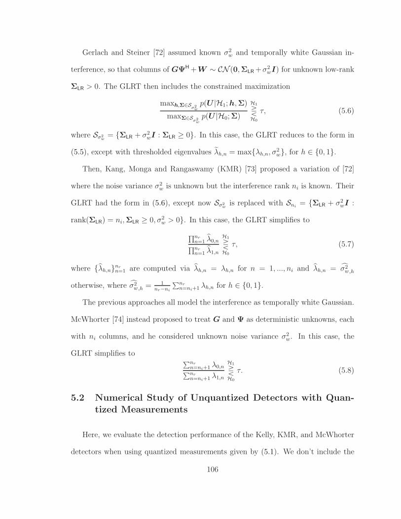
Gerlach and Steiner [72] assumed known σ2w and temporally white Gaussian in-

terference, so that columns of GΨH +W ∼ CN (0,ΣLR +σ2wI) for unknown low-rank

ΣLR > 0. The GLRT then includes the constrained maximization

maxh,Σ∈Sσ2

wp(U |H1; h,Σ)

maxΣ∈Sσ2

wp(U |H0;Σ)

H1

RH0

τ, (5.6)

where Sσ2w

= {ΣLR + σ2wI : ΣLR ≥ 0}. In this case, the GLRT reduces to the form in

(5.5), except with thresholded eigenvalues λh,n = max{λh,n, σ2w}, for h ∈ {0, 1}.

Then, Kang, Monga and Rangaswamy (KMR) [73] proposed a variation of [72]

where the noise variance σ2w is unknown but the interference rank ni is known. Their

GLRT had the form in (5.6), except now Sσ2w

is replaced with Sni= {ΣLR + σ2

wI :

rank(ΣLR) = ni,ΣLR ≥ 0, σ2w > 0}. In this case, the GLRT simplifies to

∏nrn=1 λ0,n

∏nrn=1 λ1,n

H1

RH0

τ, (5.7)

where {λh,n}nrn=1 are computed via λh,n = λh,n for n = 1, ..., ni and λh,n = σ2

w,h

otherwise, where σ2w,h = 1

nr−ni

∑nrn=ni+1 λh,n for h ∈ {0, 1}.

The previous approaches all model the interference as temporally white Gaussian.

McWhorter [74] instead proposed to treat G and Ψ as deterministic unknowns, each

with ni columns, and he considered unknown noise variance σ2w. In this case, the

GLRT simplifies to∑nr

n=ni+1 λ0,n∑nrn=ni+1 λ1,n

H1

RH0

τ. (5.8)

5.2 Numerical Study of Unquantized Detectors with Quan-

tized Measurements

Here, we evaluate the detection performance of the Kelly, KMR, and McWhorter

detectors when using quantized measurements given by (5.1). We don’t include the

106

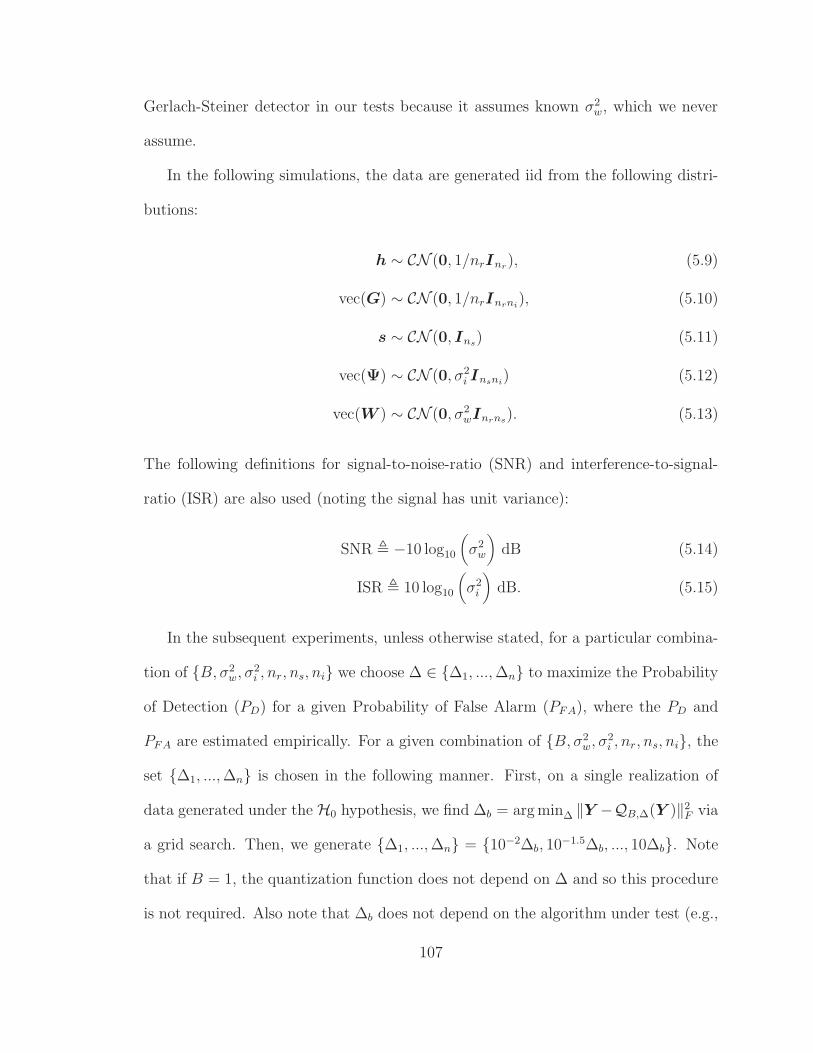
Gerlach-Steiner detector in our tests because it assumes known σ2w, which we never

assume.

In the following simulations, the data are generated iid from the following distri-

butions:

h ∼ CN (0, 1/nrInr), (5.9)

vec(G) ∼ CN (0, 1/nrInrni), (5.10)

s ∼ CN (0, Ins) (5.11)

vec(Ψ) ∼ CN (0, σ2i Insni

) (5.12)

vec(W ) ∼ CN (0, σ2wInrns). (5.13)

The following definitions for signal-to-noise-ratio (SNR) and interference-to-signal-

ratio (ISR) are also used (noting the signal has unit variance):

SNR , −10 log10

(σ2

w

)dB (5.14)

ISR , 10 log10

(σ2

i

)dB. (5.15)

In the subsequent experiments, unless otherwise stated, for a particular combina-

tion of {B, σ2w, σ2

i , nr, ns, ni} we choose ∆ ∈ {∆1, ..., ∆n} to maximize the Probability

of Detection (PD) for a given Probability of False Alarm (PFA), where the PD and

PFA are estimated empirically. For a given combination of {B, σ2w, σ2

i , nr, ns, ni}, the

set {∆1, ..., ∆n} is chosen in the following manner. First, on a single realization of

data generated under the H0 hypothesis, we find ∆b = arg min∆ ‖Y −QB,∆(Y )‖2F via

a grid search. Then, we generate {∆1, ..., ∆n} = {10−2∆b, 10−1.5∆b, ..., 10∆b}. Note

that if B = 1, the quantization function does not depend on ∆ and so this procedure

is not required. Also note that ∆b does not depend on the algorithm under test (e.g.,

107

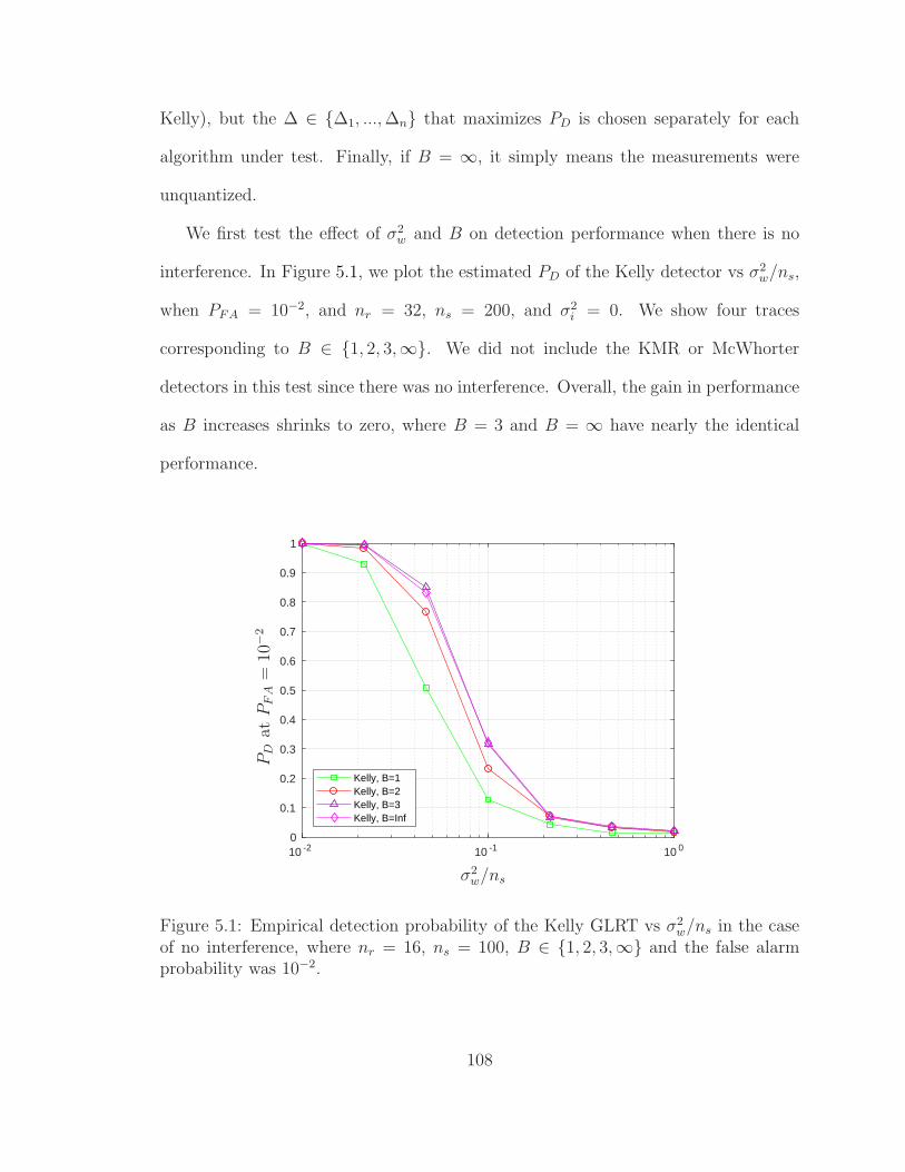
Kelly), but the ∆ ∈ {∆1, ..., ∆n} that maximizes PD is chosen separately for each

algorithm under test. Finally, if B = ∞, it simply means the measurements were

unquantized.

We first test the effect of σ2w and B on detection performance when there is no

interference. In Figure 5.1, we plot the estimated PD of the Kelly detector vs σ2w/ns,

when PFA = 10−2, and nr = 32, ns = 200, and σ2i = 0. We show four traces

corresponding to B ∈ {1, 2, 3,∞}. We did not include the KMR or McWhorter

detectors in this test since there was no interference. Overall, the gain in performance

as B increases shrinks to zero, where B = 3 and B = ∞ have nearly the identical

performance.

10 -2 10 -1 10 00

0.1

0.2

0.3

0.4

0.5

0.6

0.7

0.8

0.9

1

Kelly, B=1Kelly, B=2Kelly, B=3Kelly, B=Inf

σ2w/ns

PD

atP

FA

=10

−2

Figure 5.1: Empirical detection probability of the Kelly GLRT vs σ2w/ns in the case

of no interference, where nr = 16, ns = 100, B ∈ {1, 2, 3,∞} and the false alarmprobability was 10−2.

108

An alternate way of looking at this data is given in Figure 5.2. Here, for the same

simulation parameters used in Figure 5.1, we plot the horizontal gap between traces

of PD vs σ2w/ns (as in Figure 5.1), relative to the 1-bit trace, for different values of PD.

We refer to this gap as “SNR gain.” Calculating this gap requires linearly interpolating

the traces to obtain the corresponding σ2w values at the specified PD values (a less

quantized version of the data in Figure 5.1 was used for this purpose with more values

of B and σ2w under test, but Figure 5.1 is sufficient for seeing the big picture). Based

on this plot, increasing B from 1 to 2 has a similar effect on detection performance as

increasing the SNR by 1.5 dB in the 1-bit case. As B increases further, the marginal

gains decrease to zero, and eventually the difference in detection performance between

a detector with 1-bit and unquantized measurements is approximately equivalent to

2 dB difference in SNR.

Then, we test the effect of the interference power σ2i and bits B on detection

performance in the high SNR (low σ2w) case. In Figure 5.3 we plot the estimated

PD vs σ2i /ns of the Kelly, KMR, and McWhorter detectors when the PFA = 10−2,

nr = 16, ns = 100, ni = 1, σ2w/ns = 10−2 and B ∈ {1, 4, 8,∞}. In this case, the

KMR and McWhorter detectors were provided the true value of ni. One can see that,

in the case where B = ∞, none of the detection algorithms fail in the range of σ2i

values tested, but the detectors where B < ∞ do fail, with smaller B failing at a

lower σ2i . Also, the low-rank KMR and McWhorter detectors perform worse than the

Kelly detector. Our explanation for this behavior is that the quantization error is not

white, which is the fundamental assumption about the noise for these detectors.

Next, similar to Figure 5.2, in Figure 5.4 we plot the horizontal gap between traces

of PD vs σ2i /ns for the Kelly detector, relative to the 1-bit trace, for different values

109

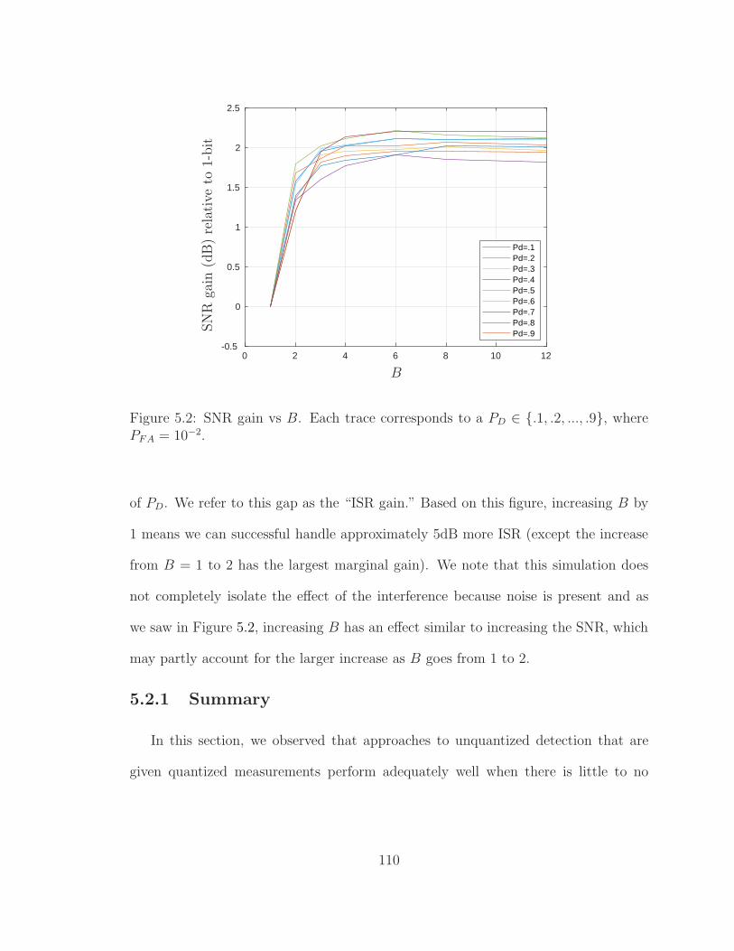
0 2 4 6 8 10 12-0.5

0

0.5

1

1.5

2

2.5

Pd=.1Pd=.2Pd=.3Pd=.4Pd=.5Pd=.6Pd=.7Pd=.8Pd=.9

B

SN

Rga

in(d

B)

rela

tive

to1-

bit

Figure 5.2: SNR gain vs B. Each trace corresponds to a PD ∈ {.1, .2, ..., .9}, wherePFA = 10−2.

of PD. We refer to this gap as the “ISR gain.” Based on this figure, increasing B by

1 means we can successful handle approximately 5dB more ISR (except the increase

from B = 1 to 2 has the largest marginal gain). We note that this simulation does

not completely isolate the effect of the interference because noise is present and as

we saw in Figure 5.2, increasing B has an effect similar to increasing the SNR, which

may partly account for the larger increase as B goes from 1 to 2.

5.2.1 Summary

In this section, we observed that approaches to unquantized detection that are

given quantized measurements perform adequately well when there is little to no

110

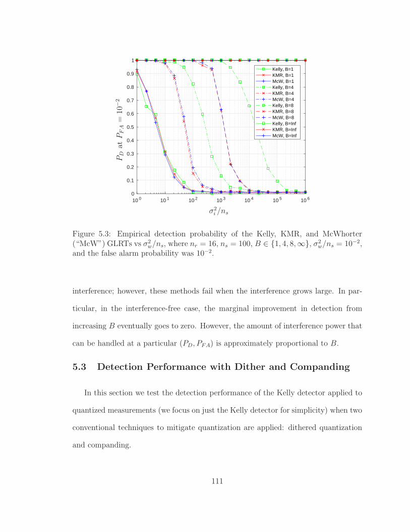
10 0 10 1 10 2 10 3 10 4 10 5 10 60

0.1

0.2

0.3

0.4

0.5

0.6

0.7

0.8

0.9

1

Kelly, B=1KMR, B=1McW, B=1Kelly, B=4KMR, B=4McW, B=4Kelly, B=8KMR, B=8McW, B=8Kelly, B=InfKMR, B=InfMcW, B=Inf

σ2i /ns

PD

atP

FA

=10

−2

Figure 5.3: Empirical detection probability of the Kelly, KMR, and McWhorter(“McW”) GLRTs vs σ2

w/ns, where nr = 16, ns = 100, B ∈ {1, 4, 8,∞}, σ2w/ns = 10−2,

and the false alarm probability was 10−2.

interference; however, these methods fail when the interference grows large. In par-

ticular, in the interference-free case, the marginal improvement in detection from

increasing B eventually goes to zero. However, the amount of interference power that

can be handled at a particular (PD, PFA) is approximately proportional to B.

5.3 Detection Performance with Dither and Companding

In this section we test the detection performance of the Kelly detector applied to

quantized measurements (we focus on just the Kelly detector for simplicity) when two

conventional techniques to mitigate quantization are applied: dithered quantization

and companding.

111

1 2 3 4 5 6 7 80

5

10

15

20

25

30

35

40

Pd=.1Pd=.2Pd=.3Pd=.4Pd=.5Pd=.6Pd=.7Pd=.8Pd=.9

B

ISR

gain

(dB

)re

lati

veto

1-bit

Figure 5.4: ISR gain vs B. Each trace corresponds to a PD ∈ {.1, .2, ..., .9}. wherePFA = 10−2.

5.3.1 Detection Performance with a Dithered Quantizer

Dither is noise added to the measured signal prior to quantization with the purpose

of altering the distribution of the quantization error. In particular, if the dither

signal’s distribution obeys certain properties, and if the quantizer does not overload,

then the quantization error, defined as the difference between the quantizer input

and output, is white and uncorrelated with the input [75]. Two commonly used

distributions for the dither signal that meet the required properties are iid uniform

dither, where dn ∼ U(−∆/2, ∆/2), and iid triangular dither, where dn = dn,1 + dn,2,

with dn,i ∼ U(−∆/2, ∆/2) and independent dn,1 and dn,2.

112

In Figure 5.5 we plot the PD of the Kelly detector vs σ2i /ns for various dither

distributions when ∆ is set so that overload within the quantizer occurred approxi-

mately .1% of the time. In this experiment B ∈ {2, 4, 6}, nr = 16, ns = 100, ni = 1,

σ2w/ns = 10−2, and PFA = 10−2. In our case with complex measurements, we gener-

ated independent dither signals for the real and imaginary channels. From this figure

we observe that the detection performance with dithering is worse than the detection

performance without dithering. Our hypothesized reason for this is that although

dither whitens the quantization error, it still increases the overall noise, which is

detrimental for detection.

10 0 10 1 10 2 10 3 10 40

0.1

0.2

0.3

0.4

0.5

0.6

0.7

0.8

0.9

1

Kelly, B=2, noneKelly, B=2, uniformKelly, B=2, triangularKelly, B=4, noneKelly, B=4, uniformKelly, B=4, triangularKelly, B=6, noneKelly, B=6, uniformKelly, B=6, triangular

σ2i /ns

PD

atP

FA

=10

−2

Figure 5.5: Estimated PD of the Kelly detector vs σ2i /ns for various dither signals,

where ∆ is set so overload occurs only a small percentage of the time. In this exper-iment nr = 16, ns = 100, ni = 1, PFA = 10−2, and σ2

w/ns = 10−2.

113

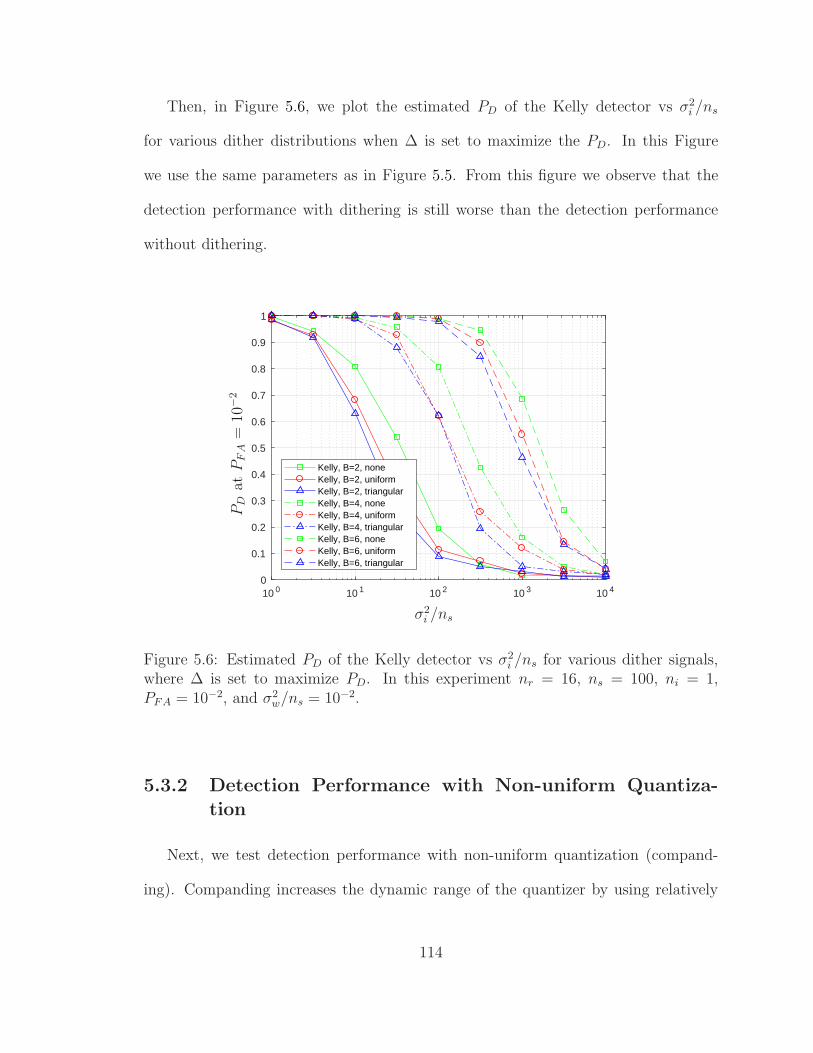
Then, in Figure 5.6, we plot the estimated PD of the Kelly detector vs σ2i /ns

for various dither distributions when ∆ is set to maximize the PD. In this Figure

we use the same parameters as in Figure 5.5. From this figure we observe that the

detection performance with dithering is still worse than the detection performance

without dithering.

10 0 10 1 10 2 10 3 10 40

0.1

0.2

0.3

0.4

0.5

0.6

0.7

0.8

0.9

1

Kelly, B=2, noneKelly, B=2, uniformKelly, B=2, triangularKelly, B=4, noneKelly, B=4, uniformKelly, B=4, triangularKelly, B=6, noneKelly, B=6, uniformKelly, B=6, triangular

σ2i /ns

PD

atP

FA

=10

−2

Figure 5.6: Estimated PD of the Kelly detector vs σ2i /ns for various dither signals,

where ∆ is set to maximize PD. In this experiment nr = 16, ns = 100, ni = 1,PFA = 10−2, and σ2

w/ns = 10−2.

5.3.2 Detection Performance with Non-uniform Quantiza-

tion

Next, we test detection performance with non-uniform quantization (compand-

ing). Companding increases the dynamic range of the quantizer by using relatively

114

precise quantization for values near 0, while allocating fewer quantization bins for

large signals. Companding can be represented mathematically by

y = f−1QB,∆

(f(x)

), (5.16)

where QB,∆ is still the uniform quantization function given in (5.2), and f is the

compressor function, and its inverse f−1 is the expander function (hence the name

companding, which is a morphing of compress and expand).

Two common choices of f are given by µ-law and A-law companding. They are

nearly identical, so for simplicity we only considered µ-law. In µ-law companding

f(x) = sgn(x)log(1 + µ|x|)log(1 + µ)

, (5.17)

where µ > 0 is a tuning parameter.

In Figure 5.7 we plot the estimated PD of the Kelly detector vs σ2i /ns with and

without µ-law companding. In this experiment, B ∈ {4, 6, 8}, nr = 16, ns = 100,

ni = 1, σ2w/ns = 10−2, and PFA = 10−2. In all cases, ∆ (and µ when companding was

applied) were optimized to maximize PD. From this Figure, we see a slight increase in

performance when companding was used, but even with companding, detection with

any level of quantization under test was eventually killed by the large interference.

5.4 The GLRT with the Quantized Model

In the previous section we saw that the performance of the Kelly detector with

quantized measurements was not significantly affected by either dithering or com-

panding. In this section we develop the GLRT for the problem in (5.1) that includes

the quantization with the goal of achieving improved detection performance, partic-

ularly in the case of strong interference.

115

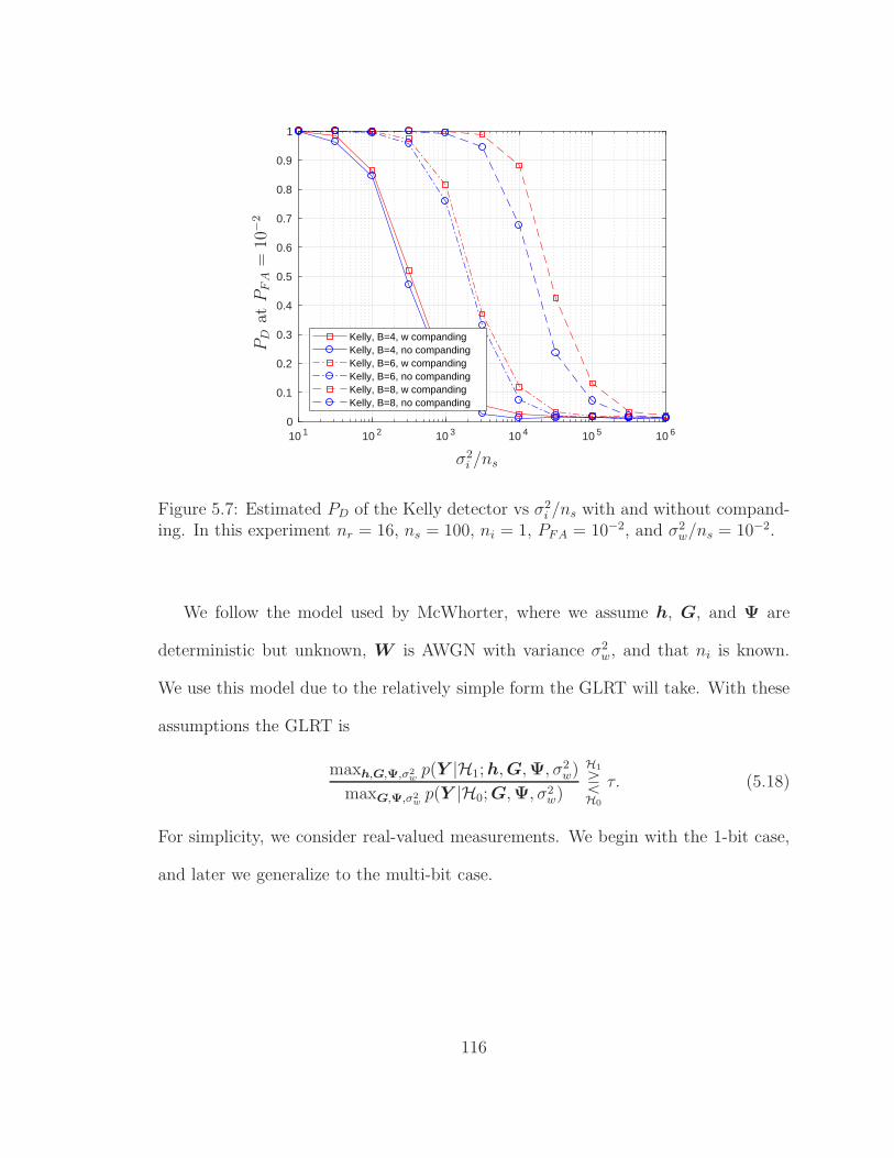
10 1 10 2 10 3 10 4 10 5 10 60

0.1

0.2

0.3

0.4

0.5

0.6

0.7

0.8

0.9

1

Kelly, B=4, w compandingKelly, B=4, no compandingKelly, B=6, w compandingKelly, B=6, no compandingKelly, B=8, w compandingKelly, B=8, no companding

σ2i /ns

PD

atP

FA

=10

−2

Figure 5.7: Estimated PD of the Kelly detector vs σ2i /ns with and without compand-

ing. In this experiment nr = 16, ns = 100, ni = 1, PFA = 10−2, and σ2w/ns = 10−2.

We follow the model used by McWhorter, where we assume h, G, and Ψ are

deterministic but unknown, W is AWGN with variance σ2w, and that ni is known.

We use this model due to the relatively simple form the GLRT will take. With these

assumptions the GLRT is

maxh,G,Ψ,σ2w

p(Y |H1; h, G,Ψ, σ2w)

maxG,Ψ,σ2w

p(Y |H0; G,Ψ, σ2w)

H1

RH0

τ. (5.18)

For simplicity, we consider real-valued measurements. We begin with the 1-bit case,

and later we generalize to the multi-bit case.

116

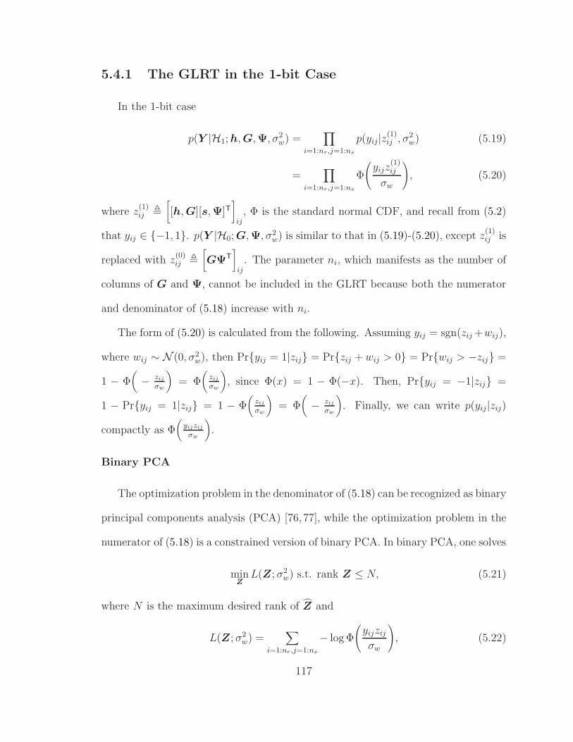
5.4.1 The GLRT in the 1-bit Case

In the 1-bit case

p(Y |H1; h, G,Ψ, σ2w) =

∏

i=1:nr ,j=1:ns

p(yij|z(1)ij , σ2

w) (5.19)

=∏

i=1:nr ,j=1:ns

Φ

(yijz

(1)ij

σw

), (5.20)

where z(1)ij ,

[[h, G][s,Ψ]T

]

ij, Φ is the standard normal CDF, and recall from (5.2)

that yij ∈ {−1, 1}. p(Y |H0; G,Ψ, σ2w) is similar to that in (5.19)-(5.20), except z

(1)ij is

replaced with z(0)ij ,

[GΨT

]

ij. The parameter ni, which manifests as the number of

columns of G and Ψ, cannot be included in the GLRT because both the numerator

and denominator of (5.18) increase with ni.

The form of (5.20) is calculated from the following. Assuming yij = sgn(zij +wij),

where wij ∼ N (0, σ2w), then Pr{yij = 1|zij} = Pr{zij + wij > 0} = Pr{wij > −zij} =

1 − Φ(− zij

σw

)= Φ

(zij

σw

), since Φ(x) = 1 − Φ(−x). Then, Pr{yij = −1|zij} =

1 − Pr{yij = 1|zij} = 1 − Φ(

zij

σw

)= Φ

(− zij

σw

). Finally, we can write p(yij|zij)

compactly as Φ(

yijzij

σw

).

Binary PCA

The optimization problem in the denominator of (5.18) can be recognized as binary

principal components analysis (PCA) [76, 77], while the optimization problem in the

numerator of (5.18) is a constrained version of binary PCA. In binary PCA, one solves

minZ

L(Z; σ2w) s.t. rank Z ≤ N, (5.21)

where N is the maximum desired rank of Z and

L(Z; σ2w) =

∑

i=1:nr,j=1:ns

− log Φ

(yijzij

σw

), (5.22)

117

which is the negative log-likelihood of the model in (5.20). Note that the optimal

value of the objective function in (5.21) is independent of σw, and therefore σw can

be assumed to equal 1.

Since the size of Z may be quite large, it is common to work with the factorization

Z = LRT and solve

minL,R

L(LRT; σ2w), (5.23)

where L and R are chosen to be of size nr ×N and ns ×N , respectively and so the

total number of optimization variables is N(nr + ns), which is smaller than nr × ns

for small enough N . Note that Problems (5.21) and (5.23) are both non-convex.

Then, to apply binary PCA to the GLRT in (5.18) with a rank constraint of ni,

the denominator of (5.18) is solved via

minG,Ψ

L(GΨT; σ2w), (5.24)

while the numerator is solved via

minh,G,Ψ

L([h, G][s,Ψ]T; σ2w), (5.25)

where in both (5.24) and (5.25), G and Ψ have ni columns. In the sequel, we will

discuss Problem (5.23) in general, where we use the notation L and R, which each

have N columns.

Regularization

Problems (5.21) and (5.23) are non-convex, and therefore difficult to solve. How-

ever, there is a convex relaxation of Problem (5.21) that leads to a regularized form

of Problems (5.24) and (5.25), which in practice may be easier to solve.

118

The convex relaxation of Problem (5.21) is to replace the rank constraint with a

nuclear-norm penalty on Z, in which case the problem is now

minZ

L(Z; σ2w) + γ‖Z‖∗, (5.26)

where γ is a tuning parameter.

Problem (5.26) is attractive compared to (5.21) because it is convex, however, in

its current form it is difficult to solve numerically due to the large number of elements

in Z. To deal with numerical difficulties we consider the Frobenius norm regularized

problem

minL,R

L(LRT; σ2w) +

γ

2

(‖L‖2F + ‖R‖2F

). (5.27)

We use this alternate form because it can be shown [77] that if (L∗, R∗) are rank N

and solve (5.27), then Z∗ = L∗R∗T solves

minZ

L(Z; σ2w) + γ‖Z‖∗ s.t. rank Z ≤ N. (5.28)

The regularization in (5.27) can be interpreted as MAP estimation of L and R

under a Gaussian prior. Indeed, if there is an independent Gaussian prior on each

element of L and R, with zero-mean and variances σ2l and σ2

r , respectively, then the

optimization problem is

minL,R

L(LRT; σ2w) +

1

2σ2l

‖L‖2F +1

2σ2r

‖R‖2F . (5.29)

Problem (5.29) depends on the parameters σ2l and σ2

r . An equivalent problem is

now presented that reduces this to a single parameter. Note that if we scale L by α

and R by 1/α, and the value of L(·) does not change. We will substitute L =√

σr

σlL

119

and R =√

σl

σrR in (5.29), yielding

= arg minL,R

L(LRT; σ2

w) +1

2

1

σlσr‖L‖2F +

1

2

1

σlσr‖R‖2F (5.30)

= arg minL,R

L(LRT; σ2

w) +γ

2

(‖l‖2F + ‖R‖2F

), (5.31)

where γ = 1σrσl

, which matches the problem in (5.27). Finally, note that L(Z; σ2w)

depends on σ2w. If we want to fix σ2

w = 1 in the optimization (as is common with

PCA), we must scale L and R each by√

σw, in which case

γ =σw

σlσr. (5.32)

Algorithms for Binary PCA

Here we describe several approaches from the literature to solving Problem (5.27).

The first, given by Collins [76], is a coordinate descent approach that loops over

elements in L and R and minimizes the objective in (5.27) wrt each scalar variable.

This process is then repeated over a number of epochs. Another approach that is

given in [78] attempts to solve Problem (5.27) via majorization-minimization. This

particular approach produces a non-increasing sequence of loss function values. A final

approach given in [77] alternates between gradient steps wrt L and R, while keeping

track of separate learning rates for each row of L and R. Regarding initialization of

L and R, all methods that have been mentioned can be initialized using the SVD

of quantized Y . This initialization typically converges to a better final value of the

objective than a random initialization [77]. In our experiments, we use the alternating

gradient descent approach in [77] combined with the SVD initialization method.

120

Gradient

Here we calculate the gradient wrt L and R of the objective in (5.23), which is

required for the alternating gradient descent algorithm in [77]. We then show a novel

quadratic approximation that improves the numerical robustness of evaluating the

gradient.

Writing

L(LRT; σ2w) = −

∑

i=1:nr,j=1:ns

log Φ(

yij∑N

n=1 linrjn

σw︸︷︷︸,aij

), (5.33)

we can calculate

d

dlin= −

∑

j

φ(aij)yij

Φ(aij)σw︸︷︷︸,fij

rjn (5.34)

and

d

drjn= −

∑

i

fijlin. (5.35)

Using (5.34) and (5.35), we can form

∇LL(LRT; σ2w) = −FR (5.36)

and

∇RL(LRT; σ2w) = −F TL. (5.37)

Quadratic Approximation for Numerical Robustness Numerical problems

arise in (5.33) when any aij are small. In order to prevent numerical problems from

occurring, we approximate the function log Φ(x) with a second-order Taylor series17

17The Feller approximation [79, 80] gives a more accurate approximation wrt absolute difference,but is not continuous at the point x0. Continuity of the spliced function and its derivative werehighly desired due to the use of gradient-descent algorithms, hence the use of a second order Taylorseries approximation.

121

about the point x0 for all x < x0. The second-order Taylor series is given by

log(Φ(x)

)

︸︷︷︸,l(x)

≈ l(x0) + l′(x0)(x− x0) +l′′(x0)

2(x− x0)

2, (5.38)

where l′(x0) = φ(x0)Φ(x0)

and l′′(x0) = −x0φ(x0)Φ(x0)−φ(x0)2

Φ(x0)2(where the latter uses the fact

that φ′(x0) = −x0φ(x0)). Then to calculate the gradient with the quadratic approxi-

mation, replace fij for all (i, j) in (5.36) and (5.37) where aij < x0 with

fij ≈(l′(x0) + l′′(x0)(aij − x0)

)yij

σw. (5.39)

In our experiments, we set x0 = −5.

Regularization If the quadratic regularization in (5.27) is used, note that

∇X

γ

2‖X‖2F = γX . (5.40)

Using this, the gradients of the regularized cost in (5.27) are

∇L

(L(LRT; σ2

w) +γ

2

(‖L‖2F + ‖R‖2F

))= −FR + γL (5.41)

and

∇R

(L(LRT; σ2

w) +γ

2

(‖L‖2F + ‖R‖2F

))= −F TL + γR. (5.42)

5.4.2 Multi-bit Case

Now we consider the GLRT in the multi-bit case.

Likelihood Function

For a given number of bits B and bin-size ∆ used in (5.2), let B = {b0, ..., b2B}

be an increasing list of numbers that correspond to the boundaries of the quantizer

122

decision regions. In this case, b0 = −∞, b2B =∞, and bi − bi−1 = ∆ for all i 6= 0, 2B.

For a given y, let b−(y) ∈ B and b+(y) ∈ B correspond to the lower and upper

boundaries, respectively, of the decision region that maps to y.

Then, p(y|z) = Pr{z + w ∈ [b−(y), b+(y)]} = Φ(

z−b−(y)σw

)− Φ

(z−b+(y)

σw

)for w ∼

N (0, σ2w). Using this, the likelihood used in the GLRT in (5.18) is

p(Y |Z; σ2w) =

∏

i=1:nr ,j=1:ns

p(yij|zij , σ2w) (5.43)

=∏

i=1:nr ,j=1:ns

Φ

(zij − b−ij

σw

)− Φ

(zij − b+

ij

σw

), (5.44)

where b−ij , b−(yij) (and likewise with +) for notational simplicity. Note that in the

case B = 1, b0 = −∞, b1 = 0, and b2 = ∞, and (5.44) corresponds to (5.20). Also

note that the dependence of p(Y |Z; σ2w) on Y manifests through the various b

+/−ij .

Now we will briefly summarize similarities and differences to the 1-bit case. First,

the quadratic regularization in (5.27) can still be used, as can the alternating gradient

descent algorithm and the SVD initialization. However, in the multi-bit case, the

optimal value of the likelihood is not invariant to the choice of σ2w, and therefore σ2

w

must be included as an estimand in the GLRT.

Gradient

Similar to the 1-bit case, we calculate the gradient of L(Z; σ2w) , − log p(Y |Z, σ2

w)

from (5.44) wrt the factors Z = LRT. We then show a novel quadratic approximation

that increases the robustness of evaluating the gradient.

Noting that

L(LRT; σ2w) =

∑

ij

− log

Φ

( ∑k likrjk − b−ij

σw︸︷︷︸,a−

ij

)− Φ

( ∑k likrjk − b+

ij

σw︸︷︷︸,a+

ij

), (5.45)

123

d

dlikL(LRT; σ2

w) = −∑

j

φ(a−ij)− φ(a+

ij)

Φ(a−ij)− Φ(a+

ij)

1

σw︸︷︷︸,fij

rjk (5.46)

and

d

drjkL(LRT; σ2

w) = −∑

i

fijlik, (5.47)

which can be written as

∇LL(LRT; σ2w) = −FR (5.48)

and

∇RL(LRT; σ2w) = −F TL. (5.49)

Quadratic Approximation for Numerical Robustness Similar to the 1-bit

case, numerical problems may arise if Φ(a−ij) − Φ(a+

ij) is very close to zero. In order

to avoid such problems, we will approximate

lij(x) , log

Φ

(x− b−ij

σw

)− Φ

(x− b+

ij

σw

) (5.50)

with a second-order Taylor series about the point x = x0 whenever x is in a range of

values that cause numerical problems.

First, we note that a second-order Taylor series is a particularly good approxima-

tion to (5.50) when there is no clipping (quantizer overload). Let x = x− b+ij . Then

after substitution,

lij(x) = log

Φ

(x + b+

ij − b−ijσw

)− Φ

(x

σw

). (5.51)

Since there is no clipping, b+ij − b−ij = ∆. Then after substitution, and for small ∆,

log

Φ

(x + ∆

σw

)− Φ

(x

σw

) ≈ log

∆

σwφ

(x

σw

) (5.52)

≈ c1x2 + c2 (5.53)

124

for constants c1 and c2.

The second order Taylor series of lij(x) about x0 (after dropping the ij subscripts

for simplicity) is given by

l(x) ≈ l(x0) + l′(x0)(x− x0) +1

2l′′(x0)(x− x0)

2, (5.54)

where

l′(x) =

1σw

(φ(

x−b−

σw

)− φ

(x−b+

σw

))

Φ(

x−b−

σw

)− Φ

(x−b+

σw

) (5.55)

and

l′′(x) =−(φ(x−)(

x−)− φ

(x+)(

x+))(

Φ(x−)− Φ

(x+))−(φ(x−)− φ

(x+))2

σ2w

(Φ(x−)− Φ

(x+))2 ,

(5.56)

where x+ , x−b+

σwand x− , x−b−

σw.

In this case where b− = −∞,

l(x) = log

(1− Φ

(x− b+

σw

)), (5.57)

l′(x) =− 1

σwφ(

x−b+

σw

)

1− Φ(

x−b+

σw

) , (5.58)

and

l′′(x) =

φ(

x−b+

σw

)(x−b+

σw

)(1− Φ

(x−b+

σw

))− φ

(x−b+

σw

)2

σ2w

1− Φ

(x−b+

σw

)

2 . (5.59)

In the case where b+ =∞,

l(x) = log Φ

(x− b−ij

σw

), (5.60)

125

l′(x) =

1σ2

wφ(

x−b−

σw

)

Φ(

x−b−

σw

) , (5.61)

and

l′′(x) =−φ

(x−b−

σw

)(x−b−

σw

)Φ(

x−b−

σw

)− φ

(x−b−

σw

)2

σ2wΦ(

x−b−

σw

)2 . (5.62)

Unlike the 1-bit case, it is more difficult to choose when to apply the Taylor series,

i.e., what vales of x trigger using the Taylor series approximation. It is also not clear

how to best choose x0. If ∆ is small, the option we recommend is to apply the Taylor

series approximation for all x, and to set x0 = yij .

5.4.3 Summary of the GLRT

Putting everything together, to evaluate the GLRT in (5.18) with a fixed ni, we

first solve

{G

(0), Ψ

(0)}= arg min

G,ΨL(GΨT; σ2

w) +γ

2

(‖G‖2F + ‖Ψ‖2F

)(5.63)

and

{h, G

(1), Ψ

(1)}= arg min

h,G,ΨL([h, G][s,Ψ]T; σ2

w) +γ

2

(‖[h, G]‖2F + ‖[s,Ψ]‖2F

), (5.64)

where in both cases G and Ψ have ni columns and we assumed σ2w = 1. Then, we

evaluate

p(Y |H1; h, G(1)

, Ψ(1)

, σ2w)

p(Y |H0; G(0)

, Ψ(0)

, σ2w)

H1

RH0

τ, (5.65)

where σ2w = 1 in both the numerator and denominator of (5.65).

5.4.4 Numerical Results

In this section we evaluate the performance of the quantized GLRT. First, in

Figure 5.8, we plot the estimated PD of various detectors vs σ2i /ns in the one-bit

126

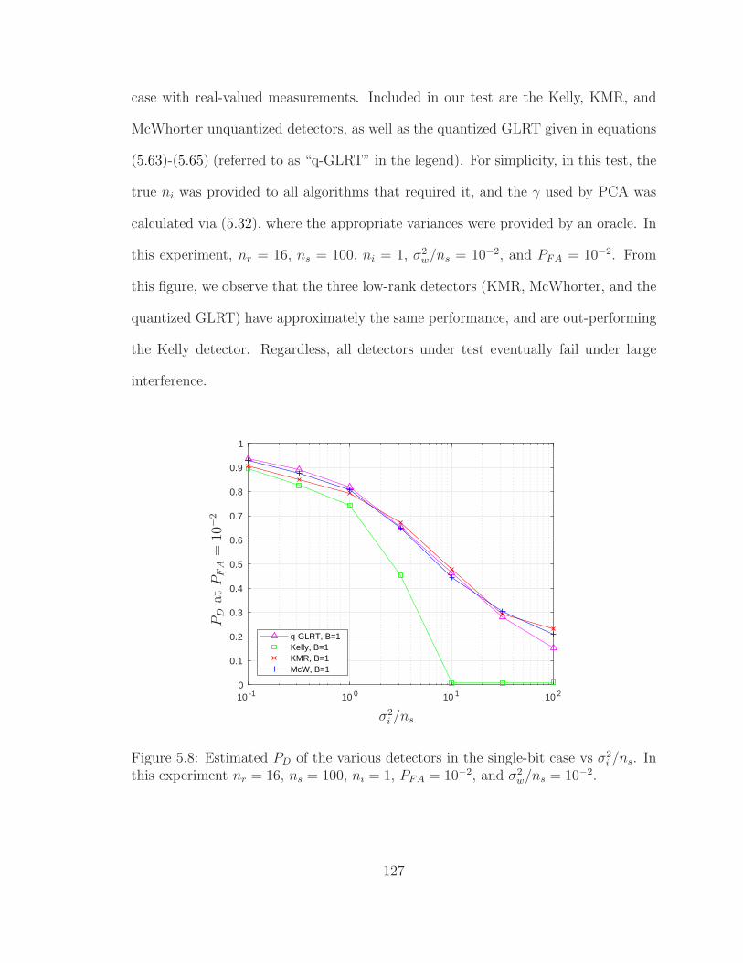
case with real-valued measurements. Included in our test are the Kelly, KMR, and

McWhorter unquantized detectors, as well as the quantized GLRT given in equations

(5.63)-(5.65) (referred to as “q-GLRT” in the legend). For simplicity, in this test, the

true ni was provided to all algorithms that required it, and the γ used by PCA was

calculated via (5.32), where the appropriate variances were provided by an oracle. In

this experiment, nr = 16, ns = 100, ni = 1, σ2w/ns = 10−2, and PFA = 10−2. From

this figure, we observe that the three low-rank detectors (KMR, McWhorter, and the

quantized GLRT) have approximately the same performance, and are out-performing

the Kelly detector. Regardless, all detectors under test eventually fail under large

interference.

10 -1 10 0 10 1 10 20

0.1

0.2

0.3

0.4

0.5

0.6

0.7

0.8

0.9

1

q-GLRT, B=1Kelly, B=1KMR, B=1McW, B=1

σ2i /ns

PD

atP

FA

=10

−2

Figure 5.8: Estimated PD of the various detectors in the single-bit case vs σ2i /ns. In

this experiment nr = 16, ns = 100, ni = 1, PFA = 10−2, and σ2w/ns = 10−2.

127

Then, in Figure 5.9, we examine performance as B is increased. We plot empirical

receiver operating characteristic (ROC) curves (which show PD as a function of PFA)

for various detectors and B ∈ {1, 2, 3,∞}. In this experiment nr = 16, ns = 100,

ni = 1, σ2w/ns = 10−2, and σ2

i /ns = 1. As before, the true value of ni was provided

to all detectors that required it, and the γ used by PCA was again calculated via

(5.32), where the appropriate variances were provided by an oracle. Note that the

quantized GLRT cannot be evaluated when B = ∞. From this figure, we see that

performance for all detectors improves as B increases. The relative performance

between the detectors is Kelly is the worst, followed by the KMR detector, and

finally the quantized GLRT and McWhorter are approximately tied for the best.

10 -3 10 -2 10 -1

0.5

0.55

0.6

0.65

0.7

0.75

0.8

0.85

0.9

0.95

q-GLRT, B=1Kelly, B=1KMR, B=1McW, B=1q-GLRT, B=2Kelly, B=2KMR, B=2McW, B=2q-GLRT, B=3Kelly, B=3KMR, B=3McW, B=3Kelly, B=infKMR, B=infMcW, B=inf

PFA

PD

Figure 5.9: Estimated ROC curves of various detectors for different values of B. Inthis experiment nr = 16, ns = 100, ni = 1, σ2

i /ns = 1, and σ2w/ns = 10−2.

128

5.4.5 Summary

In this section we developed the GLRT for the quantized model in the case of real-

valued measurements. Based on the assumptions we made regarding G, Ψ, and W ,

the two estimation problems in the GLRT involve PCA from quantized measurements,

which is a particular example of generalized bilinear inference. While we admit there

is future work that could be performed in this area, including: extension to the

complex case, incorporating optimization of σ2w in the multi-bit case, and applying

other generalized low-rank inference algorithms such as low-rank AMP (LowRAMP)

[7] or Bilinear GAMP (BiGAMP) [6], with our work so far there is not evidence that it

will improve detection significantly in the high interference case, which is the regime

of interest (although the PCA-based GLRT may offer a slight improvement over the

Kelly detector). Therefore, in the next section we again turn to alternate techniques

to improve detection performance in the case of high interference.

5.5 Pre-processing Techniques

So far, we have observed the general trend that detection from quantized mea-

surement performs adequately well when the interference is small, but suffers from a

lack of dynamic range when the interference is large. Techniques such as dithering,

companding, or the GLRT with the quantized model have been of limited value, and

so in this section we explore alternative ways of quantizing the signal.

We note the various approaches we propose in the sequel require a significant

change of the receiver architecture. Some methods require a matrix multiplication

of the received signal prior to quantization, which may not be feasible in practice,

but we consider them anyway as a point of comparison. In light of this, we also test

129

more “implementable” approaches, where the matrix multiplication consists of unit-

modulus elements (i.e., the only operations are phase-shifting and adding), which can

be implemented more easily in the analog domain.

5.5.1 Beamforming

We first consider beamforming. In beamforming, at each time snapshot the

received signal from each antenna are linearly combined via beamforming vector

b ∈ Cnr , prior to quantization. This can be written as

y = QB,∆

(UHb

)∈ C

ns , (5.66)

where the detection statistic is computed from y instead of U or QB,∆(U). Note that

UHb = shHb + ΨGHb + W Hb, (5.67)

which, under the assumption of white, Gaussian Ψ and W , is equivalent to

UHb = hs + n, (5.68)

where h is an unknown, complex gain and n is AWGN with unknown variance σ2n.

The appropriate GLRT to apply to (5.68) is therefore

maxh,σ2np(y|H1; h, σ2

n)

maxσ2np(y|H0; σ2

n)

H1

RH0

τ, (5.69)

which simplifies to

‖y‖2‖yP⊥

s ‖2H1

RH0

τ. (5.70)

Now we discuss various approaches to designing b. As mentioned before, we

consider approaches with and without regard to practicality of the implementation.

130

The first method is the well known Capon beamformer, which maximizes the signal

to interference plus noise ratio (SINR). Given h and Σ , Cov{Y},

bcapon = Σ−1h. (5.71)

Then, with implementation in mind, Smith [81] provides a conjugate-gradient algo-

rithm that, given h and Σ, yields the “Capon-phase” beamformer bcapon-phase that

maximizes the SINR after beamforming while restricting elements in bcapon-phase to

unit-modulus.

Now we test the performance of these detection methods. In Figure 5.10 we

plot the estimated PD vs σ2i /ns for a fixed PFA = 10−2. In this test, nr = 16,

ns = 100, ni = 1, and σ2w/ns = 10−2. Included in our test is the detector in (5.70)

applied to the output of (5.66) in the case of Capon beamforming and “Capon-phase”

beamforming, and also the Kelly detector applied to the quantized measurements

without beamforming. In this test, B = 3, and as usual ∆ was chosen for each

approach to maximize the estimated PD. The Capon and Capon-phase beamformers

used ML estimates of h and Σ, computed from U generated under H1. In this figure,

the Capon approach worked perfectly for all levels of interference. The Capon-phase

approach worked well, but eventually started to degrade for high levels of interference.

5.5.2 Pre-Whitening

In this section we consider approaches based on estimating Σ from quantized

measurements and adjusting the pre-processing accordingly. In particular, if we can

estimate Σ, we would like to pre-whiten18 the signal prior to quantization. We pro-

pose an iterative method that updates the whitening operation using the estimated

18For reference, if Cov{u} = Σ, then Cov{Ru} = I if RHR = Σ−1. Here R has no relation tothe R in Section 5.4.

131

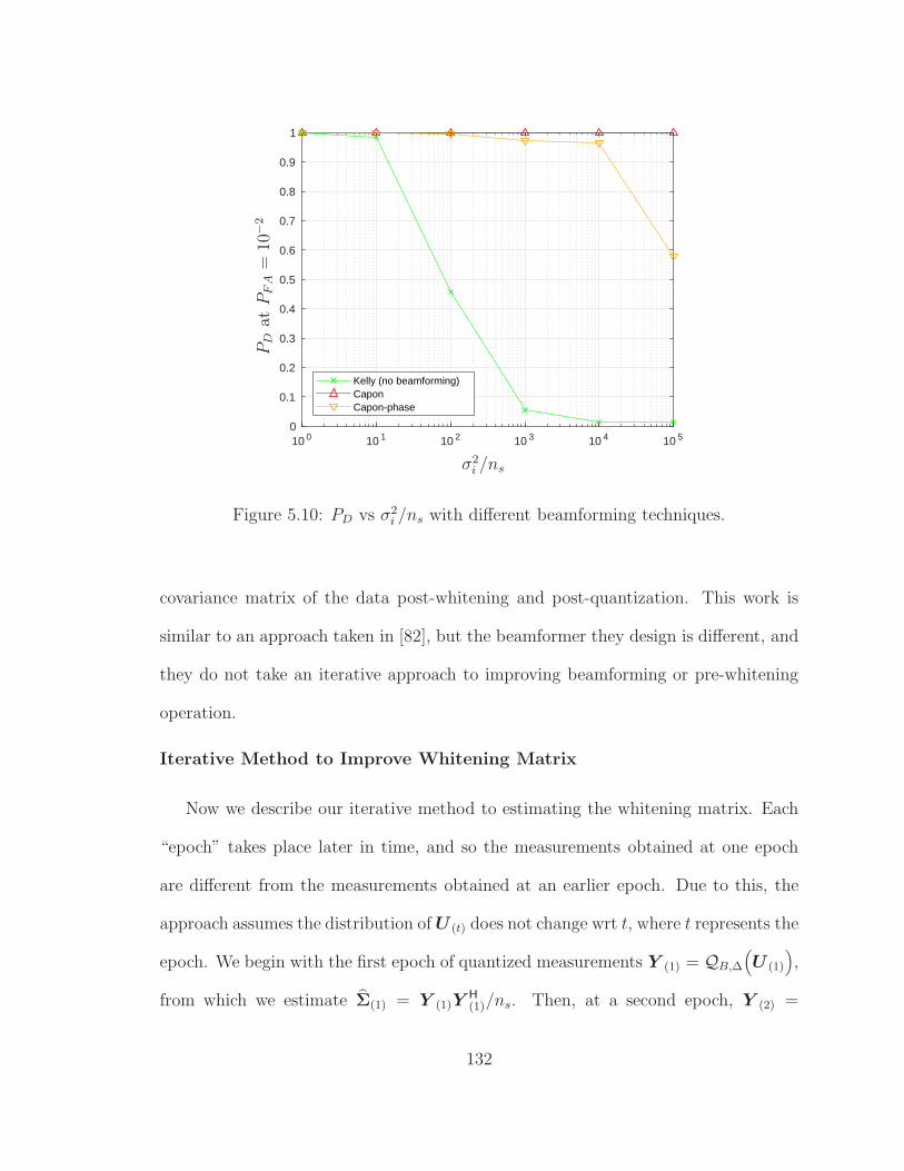
10 0 10 1 10 2 10 3 10 4 10 50

0.1

0.2

0.3

0.4

0.5

0.6

0.7

0.8

0.9

1

Kelly (no beamforming)CaponCapon-phase

σ2i /ns

PD

atP

FA

=10

−2

Figure 5.10: PD vs σ2i /ns with different beamforming techniques.

covariance matrix of the data post-whitening and post-quantization. This work is

similar to an approach taken in [82], but the beamformer they design is different, and

they do not take an iterative approach to improving beamforming or pre-whitening

operation.

Iterative Method to Improve Whitening Matrix

Now we describe our iterative method to estimating the whitening matrix. Each

“epoch” takes place later in time, and so the measurements obtained at one epoch

are different from the measurements obtained at an earlier epoch. Due to this, the

approach assumes the distribution of U (t) does not change wrt t, where t represents the

epoch. We begin with the first epoch of quantized measurements Y (1) = QB,∆

(U (1)

),

from which we estimate Σ(1) = Y (1)YH(1)/ns. Then, at a second epoch, Y (2) =

132

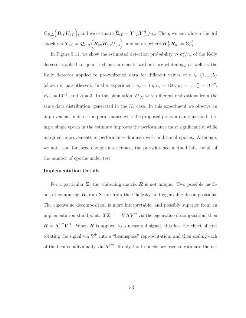
QB,∆

(R(1)U (2)

), and we estimate Σ(2) = Y (2)Y

H(2)/ns. Then, we can whiten the 3rd

epoch via Y (3) = QB,∆

(R(2)R(1)U (3)

), and so on, where RH

(t)R(t) = Σ−1

(t) .

In Figure 5.11, we show the estimated detection probability vs σ2i /ns of the Kelly

detector applied to quantized measurements without pre-whitening, as well as the

Kelly detector applied to pre-whitened data for different values of t ∈ {1, ..., 5}

(shown in parentheses). In this experiment, nr = 16, ns = 100, ni = 1, σ2w = 10−2,

PFA = 10−2, and B = 3. In this simulation, U (t) were different realizations from the

same data distribution, generated in the H0 case. In this experiment we observe an

improvement in detection performance with the proposed pre-whitening method. Us-

ing a single epoch in the estimate improves the performance most significantly, while

marginal improvements in performance diminish with additional epochs. Although,

we note that for large enough interference, the pre-whitened method fails for all of

the number of epochs under test.

Implementation Details

For a particular Σ, the whitening matrix R is not unique. Two possible meth-

ods of computing R from Σ are from the Cholesky and eigenvalue decompositions.

The eigenvalue decomposition is more interpretable, and possibly superior from an

implementation standpoint. If Σ−1 = V ΛV H via the eigenvalue decomposition, then

R = Λ1/2V H. When R is applied to a measured signal, this has the effect of first

rotating the signal via V H into a “beamspace” representation, and then scaling each

of the beams individually via Λ1/2. If only t = 1 epochs are used to estimate the net

133

R, it is possible to implement the Λ1/2 action by adjusting the gains on the individ-

ual ADCs (similar to companding19), prior to applying Λ1/2 to the post-quantized

samples, in which case the only thing that needs to be implemented in the analog

domain is the rotation V H. Specifically,

QB,∆

(Λ1/2V Hu

)= Λ1/2QB,Λ−1/2∆

(V Hu

), (5.72)

where QB,Λ−1/2∆(·) has channel-wise ∆i = λ−1/2i ∆. However, if t > 1 epochs are used,

it is unclear if the action of all Λ1/2(t) can be incorporated in the quantizer, because

the overall whitening plus quantization operation is

QB,∆

(Λ

1/2(t) V H

(t)...Λ1/2(1) V H

(1)u

). (5.73)

One area of future work is to see if the net whitening operation with an arbitrary

number of epochs is able to be written (or approximated) as a single rotation followed

by a channel-wise scaling. In the sequel we observe what happens when we restrict

V (t) to unit modulus elements, which can then be implemented the the analog domain

more efficiently.

Implementation with Unit-modulus Elements

A simple approach to implementing the whitening filter with phase-shifters only

is to replace elements in V with vij = vij/|vij|. On top of that, if only discrete phases

are allowed, the argument of vij can be quantized to one of the allowed phases. A

justification for this approach is now given. The rows of V H indicate the direction

of each “beam”. We want to replace rows of V H with vectors that are as parallel

19In companding, the same non-uniform quantization function is used on every ADC, whereashere each ADC uses a uniform quantization function but with ADC-dependent ∆.

134

10 0 10 1 10 2 10 3 10 4 10 5 10 60

0.1

0.2

0.3

0.4

0.5

0.6

0.7

0.8

0.9

1

Kelly (no beamformingiterative whitening (1)iterative whitening (2)iterative whitening (3)iterative whitening (4)iterative whitening (5)

σ2i /ns

PD

atP

FA

=10

−2

Figure 5.11: PD vs σ2i /ns with iterative whitening technique. Number in parentheses

shows number of iterations (epochs).

as possible while being restricted to unit-modulus elements. This problem can be

written as

vi = arg maxv

vHi v s.t. |vj| = 1∀j, (5.74)

where vHi is the ith row of V H. From this problem, it is clear the solution is vij =

vij/|vij| for all i and j.

In Figures 5.12 and 5.13, we evaluate the performance of the proposed itera-

tive whitening method when elements in V are restricted to unit modulus and unit

modulus with discrete phases, respectively. We used the same parameters as in the

experiment in Figure 5.11. We observe a moderate performance loss when compar-

ing to the phase only performance in Figure 5.12 to the arbitrary V performance in

Figure 5.11. Then, there is a small performance loss when comparing the phase only

135

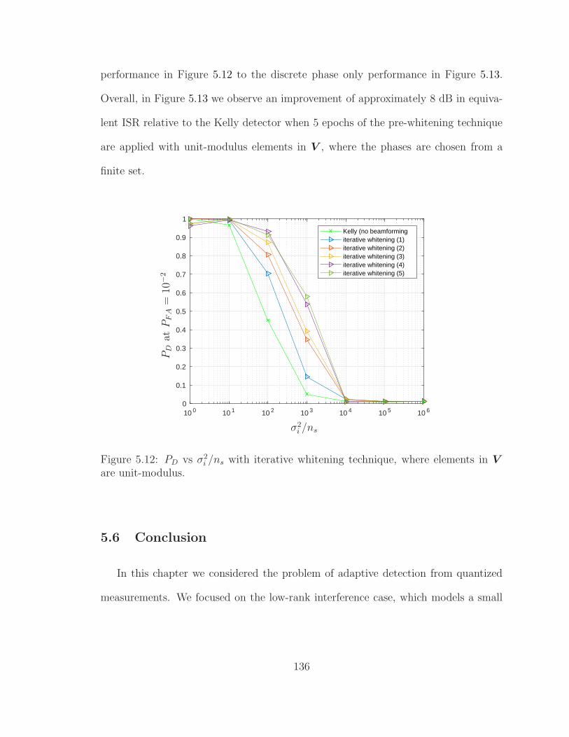
performance in Figure 5.12 to the discrete phase only performance in Figure 5.13.

Overall, in Figure 5.13 we observe an improvement of approximately 8 dB in equiva-

lent ISR relative to the Kelly detector when 5 epochs of the pre-whitening technique

are applied with unit-modulus elements in V , where the phases are chosen from a

finite set.

10 0 10 1 10 2 10 3 10 4 10 5 10 60

0.1

0.2

0.3

0.4

0.5

0.6

0.7

0.8

0.9

1


σ2i /ns

PD

atP

FA

=10

−2

Figure 5.12: PD vs σ2i /ns with iterative whitening technique, where elements in V

are unit-modulus.

5.6 Conclusion

In this chapter we considered the problem of adaptive detection from quantized

measurements. We focused on the low-rank interference case, which models a small

136

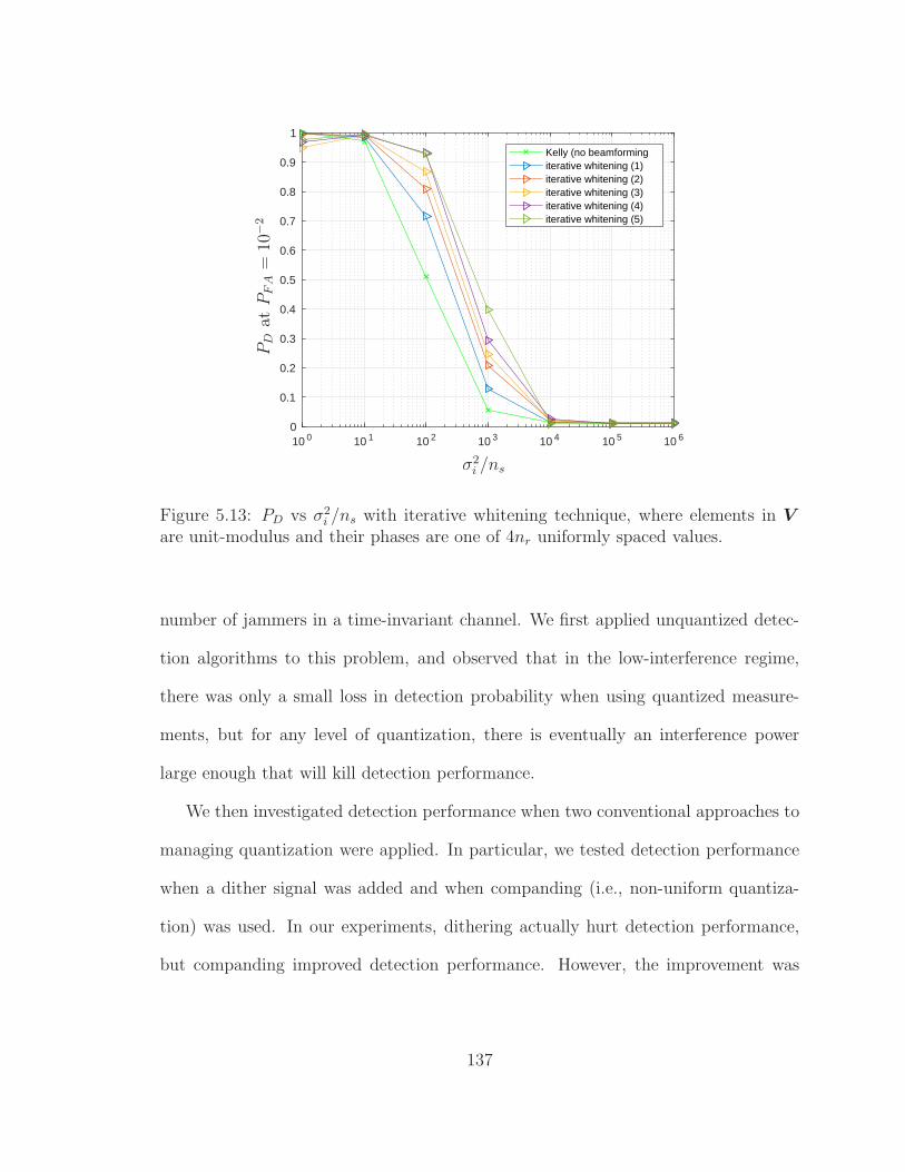
10 0 10 1 10 2 10 3 10 4 10 5 10 60

0.1

0.2

0.3

0.4

0.5

0.6

0.7

0.8

0.9

1


σ2i /ns

PD

atP

FA

=10

−2

Figure 5.13: PD vs σ2i /ns with iterative whitening technique, where elements in V

are unit-modulus and their phases are one of 4nr uniformly spaced values.

number of jammers in a time-invariant channel. We first applied unquantized detec-

tion algorithms to this problem, and observed that in the low-interference regime,

there was only a small loss in detection probability when using quantized measure-

ments, but for any level of quantization, there is eventually an interference power

large enough that will kill detection performance.

We then investigated detection performance when two conventional approaches to

managing quantization were applied. In particular, we tested detection performance

when a dither signal was added and when companding (i.e., non-uniform quantiza-

tion) was used. In our experiments, dithering actually hurt detection performance,

but companding improved detection performance. However, the improvement was

137

small, and still did not prevent large interference from eventually killing detection

performance.

Then, we developed the GLRT that assumed quantization. The GLRT for our

quantized model involves solving two generalized bilinear inference problems. How-

ever, the overall detection performance of this GLRT was not good enough relative

to simply applying unquantized detectors to quantized data to justify continuing its

development.

In the final section of this chapter we applied various pre-processing techniques to

the signal to effectively try to null the interference prior to quantization. We observed

that methods that know the true interference plus noise covariance matrix are able

to significantly improve detection performance, but they are not practical because in

practice the true interference plus noise covariance matrix is unknown. In response, we

developed an iterative technique for estimating the interference plus noise covariance

matrix, and using this to apply a whitening filter prior to quantization. The whitening

filter can then be iteratively improved over time as more measurements are taken.

This approach offered the best improvement in detection performance in the high

interference case relative to all of the techniques under evaluation.

138

Chapter 6: Conclusion

In this dissertation we considered various problems that involve inference in the

generalized linear model. Specifically, we considered the multinomial logistic regres-

sion and the sketched clustering problems. In both applications, we applied the

HyGAMP algorithm to estimate the underlying parameters of interest. Then, through

numerical simulations on synthetic and real-world datasets, we demonstrated that our

approximate message passing approach to inference outperformed existing state-of-

the-art approaches based on optimization for inference in both accuracy and compu-

tational complexity.

Then, in the final chapter of this dissertation we considered the problem of adap-

tive detection from quantized measurements, while focusing on the low-rank inter-

ference case. We first studied the performance of unquantized detection approaches

when they were given quantized measurements. We observed these unquantized tech-

niques work well in the low interference case but not the high interference case. We

then investigated various approaches to improving the detection performance in the

high interference regime. We first considered approaches such has applying a dither

signal or using non-uniform quantization (companding). Then, we derived and im-

plemented the GLRT with the quantized model, which we gave rise to the generalized

bilinear model. Another final method that we considered was to whiten the data prior

139

to quantization using processing in the analog domain. Our particular approach used

feedback from the output of the quantizer to design the analog whitening operation.

Through numerical experiments, we observed this approach had the best improvement

over among all approaches that were considered.

140

Bibliography

[1] D. L. Donoho, A. Maleki, and A. Montanari, “Message passing algorithms forcompressed sensing,” Proc. National Academy of Sciences, vol. 106, no. 45, pp.

18 914–18 919, Nov. 2009.

[2] S. Rangan, “Generalized approximate message passing for estimation with ran-

dom linear mixing,” in Proc. IEEE Internat. Symposium on Information Theory,Aug. 2011, pp. 2168–2172, (full version at arXiv:1010.5141 ).

[3] M. Bayati and A. Montanari, “The dynamics of message passing on dense graphs,with applications to compressed sensing,” IEEE Trans. on Information Theory,

vol. 57, no. 2, pp. 764–785, Feb. 2011.

[4] J. P. Vila and P. Schniter, “Expectation-maximization Gaussian-mixture approx-

imate message passing,” IEEE Trans. on Signal Processing, vol. 61, no. 19, pp.4658–4672, Oct. 2013.

[5] S. Rangan, A. K. Fletcher, V. K. Goyal, E. Byrne, and P. Schniter, “Hybridapproximate message passing,” IEEE Trans. on Signal Processing, vol. 65, no. 17,

pp. 4577–4592, 2017.

[6] J. T. Parker, P. Schniter, and V. Cevher, “Bilinear generalized approximate

message passing—Part I: Derivation,” IEEE Trans. on Signal Processing, vol. 62,no. 22, pp. 5839–5853, Nov. 2014.

[7] T. Lesieur, F. Krzakala, and L. Zdeborova, “MMSE of probabilistic low-

rank matrix estimation: Universality with respect to the output channel,”

arXiv:1507.03857, Jan. 2016.

[8] T. Lesieur, F. Krzakala, and L. Zdeborov, “Constrained low-rank matrix es-timation: Phase transitions, approximate message passing and applications,”

Journal of Statistical Mechanics: Theory and Experiment, vol. 2017, no. 7, p.

073403, 2017.

[9] E. M. Byrne and P. Schniter, “Sparse multinomial logistic regression via approx-imate message passing,” IEEE Trans. on Signal Processing, vol. 64, no. 21, pp.

5485–5498, 2016.

141

[10] B. Krishnapuram, L. Carin, M. Figueiredo, and A. Hartemink, “Sparse multi-nomial logistic regression: Fast algorithms and generalization bounds,” IEEE

Trans. on Pattern Analysis and Machine Intelligence, vol. 27, no. 6, pp. 957–968, Jun. 2005.

[11] N. Keriven, A. Bourrier, R. Gribonval, and P. Perez, “Sketching for large-scalelearning of mixture models,” in Proc. IEEE Internat. Conf. on Acoustics, Speech,

and Signal Processing, 2016, pp. 6190–6194.

[12] N. Keriven, N. Tremblay, Y. Traonmilin, and R. Gribonval, “Compressive K-

means,” arXiv:1610.08738, 2016.

[13] S. Rangan, A. K. Fletcher, V. K. Goyal, and P. Schniter, “Hybrid generalized

approximate message passing with applications to structured sparsity,” in Proc.

IEEE Internat. Symposium on Information Theory, Jul. 2012, pp. 1236–1240,(full version at arXiv:1111.2581 ).

[14] E. M. Byrne, “Sparse multinomial logistic regression via approximate messagepassing,” Master’s thesis, The Ohio State University, Columbus, Ohio, July 2015.

[15] H. Sun et al., “Neuronal and glioma-derived stem cell factor induces angiogenesiswithin the brain,” Cancer Cell, vol. 9, pp. 287–300, 2006.

[16] A. Bhattacharjee et al., “Classification of human lung carcinomas by mRNAexpression profiling reveals distinct adenocarcinoma subclasses,” Proc. National

Academy of Sciences, vol. 98, pp. 13 790–13 795, Nov 2001.

[17] J. Haxby, M. Gobbini, M. Furey, A. Ishai, J. Schouten, and P. Pietrini, “Dis-

tributed and overlapping representations of faces and objects in ventral temporal

cortex,” Science, vol. 293, pp. 2425–2430, 2001.

[18] K. A. Norman, S. M. Polyn, G. J. Detre, and J. V. Haxby, “Beyond mind-reading:

multi-voxel pattern analysis of fMRI data,” Trends in Cognitive Sciences, vol. 10,no. 9, pp. 424–430, Sep. 2006.

[19] G. Forman, “An extensive empirical study of feature selection metrics for textclassification,” J. Mach. Learn. Res., vol. 3, pp. 1289–1305, 2003.

[20] D. Lewis, Y. Yang, T. Rose, and F. Li, “RCV1: A new benchmark collection fortext categorization research,” Journal of Machine Learning Research, vol. 5, pp.

361–397, Apr. 2004.

[21] A. Gustafsson, A. Hermann, and F. Huber, Conjoint Measurement: Methods and

Applications. Berlin: Springer-Verlag, 2007.

142

[22] Y. Plan and R. Vershynin, “Robust 1-bit compressed sensing and sparse logis-tic regression: A convex programming approach,” IEEE Trans. on Information

Theory, vol. 59, no. 1, pp. 482–494, 2013.

[23] C. M. Bishop, Pattern Recognition and Machine Learning. New York: Springer,2007.

[24] M. E. Tipping, “Sparse Bayesian learning and the relevance vector machine,”

Journal of Machine Learning Research, vol. 1, pp. 211–244, 2001.

[25] A. Genkin, D. D. Lewis, and D. Madigan, “Large-scale Bayesian logistic regres-sion for text categorization,” Technometrics, vol. 49, no. 3, pp. 291–304, Aug.

2007.

[26] J. Friedman, T. Hastie, and R. Tibshirani, “Regularization paths for generalizedlinear models via coordinate descent,” J. Statst. Softw., vol. 33, no. 1, pp. 1–22,

Jan. 2010.

[27] G. C. Cawley, N. L. C. Talbot, and M. Girolami, “Sparse multinomial logistic re-gression via Bayesian L1 regularisation,” in Proc. Neural Information Processing

Systems Conf., 2007, pp. 209–216.

[28] L. Meier, S. van de Geer, and P. Buhlmann, “The group lasso for logistic re-

gression,” Journal of the Royal Statistical Society: Series B, vol. 70, pp. 53–71,2008.

[29] Y. Grandvalet, “Least absolute shrinkage is equivalent to quadratic penaliza-

tion,” in Proc. Internat. Conf. Artificial on Neural Networks, 1998, pp. 201–206.

[30] D. J. C. MacKay, “The evidence framework applied to classification networks,”Neural Computation, vol. 4, pp. 720–736, 1992.

[31] J. Pearl, Probabilistic Reasoning in Intelligent Systems. San Mateo, CA: Morgan

Kaufman, 1988.

[32] J. Ziniel, P. Schniter, and P. Sederberg, “Binary classification and feature se-lection via generalized approximate message passing,” IEEE Trans. on Signal

Processing, vol. 63, no. 8, pp. 2020–2032, 2015.

[33] D. L. Donoho, A. Maleki, and A. Montanari, “Message passing algorithms forcompressed sensing: I. Motivation and construction,” in Proc. Information The-

ory Workshop, Cairo, Egypt, Jan. 2010, pp. 1–5.

[34] D. A. Knowles and T. P. Minka, “Non-conjugate variational message passingfor multinomial and binary regression,” in Proc. Neural Information Processing

Systems Conf., 2011, pp. 1701–1709.

143

[35] A. Mousavi, A. Maleki, and R. G. Baraniuk, “Parameterless, optimal approxi-mate message passing,” arXiv:1311.0035, Nov. 2013.

[36] G. F. Cooper, “The computational complexity of probabilistic inference usingBayesian belief networks,” Artificial Intelligence, vol. 42, pp. 393–405, 1990.

[37] A. Javanmard and A. Montanari, “State evolution for general approximate mes-sage passing algorithms, with applications to spatial coupling,” Information and

Inference, vol. 2, no. 2, pp. 115–144, 2013.

[38] S. Rangan, P. Schniter, E. Riegler, A. Fletcher, and V. Cevher, “Fixed points

of generalized approximate message passing with arbitrary matrices,” in Proc.IEEE Internat. Symposium on Information Theory, Jul. 2013, pp. 664–668, (full

version at arXiv:1301.6295 ).

[39] S. Rangan, P. Schniter, and A. Fletcher, “On the convergence of generalizedapproximate message passing with arbitrary matrices,” in Proc. IEEE Inter-

nat. Symposium on Information Theory, Jul. 2014, pp. 236–240, (preprint atarXiv:1402.3210 ).

[40] R. Tibshirani, “Regression shrinkage and selection via the lasso,” Journal of theRoyal Statistical Society: Series B, vol. 58, no. 1, pp. 267–288, 1996.

[41] D. R. Hunter and K. Lange, “A tutorial on MM algorithms,” The AmericanStatistician, vol. 58, no. 1, pp. 30–37, 2004.

[42] D. Hunter and R. Li, “Variable selection using MM algorithms,” Annals of Statis-tics, vol. 33, no. 4, pp. 1617–1642, 2005.

[43] D. Bertsekas, Nonlinear Programming, 2nd ed. Athena Scientific, 1999.

[44] D. Bohning, “Multinomial logistic regression algorithm,” Ann. Inst. Statist.Math., vol. 44, pp. 197–200, 1992.

[45] P. Schniter, “Turbo reconstruction of structured sparse signals,” in Proc. Conf.on Information Science and Systems, Princeton, NJ, Mar. 2010, pp. 1–6.

[46] L. A. Stefanski, “A normal scale mixture representation of the logistic distribu-tion,” Stats. Prob. Letters, vol. 11, no. 1, pp. 69–70, 1991.

[47] C. E. Rasmussen and C. K. I. Williams, Gaussian Processes for Machine Learn-ing. Cambridge, MA: MIT Press, 2006.

[48] C. M. Stein, “Estimation of the mean of a multivariate normal distribution,”Annals of Statistics, vol. 9, pp. 1135–1151, 1981.

144

[49] M. I. Jordan, “Why the logistic function? A tutorial discussion on probabilitiesand neural networks,” MIT, Computational Cognitive Science, Tech. Rep. 9503,

1995.

[50] Y. LeCun, L. Bottou, Y. Bengio, and P. Haffner, “Gradient-based learning ap-

plied to document recognition,” in Proceedings of the IEEE, vol. 86, Nov. 1998,pp. 2278–2324.

[51] P. Drineas, A. Frieze, R. Kannan, S. Vempala, and V. Vinay, “Clustering largegraphs via the singular value decomposition,” Machine Learning, vol. 56, no. 1-3,

pp. 9–33, 2004.

[52] H. Steinhaus, “Sur la division des corps materiels en parties,” Bulletin de lAcad-

mie Polonaise des Sciences, vol. 4, no. 12, pp. 801–804, 1956.

[53] A. K. Jain, “Data clustering: 50 years beyond K-means,” Pattern RecognitionLetters, vol. 31, no. 8, pp. 651–666, Jun. 2010.

[54] D. Arthur and S. Vassilvitskii, “k-means++: The advantages of careful seeding,”in Proc. ACM-SIAM Symposium on Discrete Algorithms, 2007, pp. 1027–1035.

[55] N. Keriven, A. Bourrier, R. Gribonval, and P. Perez, “Sketching for large-scalelearning of mixture models,” Information and Inference, vol. 7, no. 3, pp. 447–

508, 2017.

[56] N. Keriven, N. Tremblay, Y. Traonmilin, and R. Gribonval, “Compressive K-

means,” in Proc. IEEE Internat. Conf. on Acoustics, Speech, and Signal Pro-cessing, 2017, pp. 6369–6373.

[57] R. Gribonval, G. Blanchard, N. Keriven, and Y. Traonmilin, “Compressive sta-

tistical learning with random feature moments,” arXiv:1706.07180, 2017.

[58] A. Feuerverger and R. A. Mureika, “The empirical characteristic function and

its applications,” Annals of Statistics, vol. 5, no. 1, pp. 88–97, 1977.

[59] Y. C. Pati, R. Rezaiifar, and P. S. Krishnaprasad, “Orthogonal matching pursuit:

Recursive function approximation with applications to wavelet decomposition,”in Proc. Asilomar Conf. on Signals, Systems and Computers, Pacific Grove, CA,

1993, pp. 40–44.

[60] P. McCullagh and J. A. Nelder, Generalized Linear Models, 2nd ed. London:

Chapman & Hall/CRC, 1989.

[61] A. Papoulis, Probability, Random Variables, and Stochastic Processes, 3rd ed.

New York: McGraw-Hill, 1991.

145

[62] M. Rudelson and R. Vershynin, “Hanson-Wright inequality and sub-Gaussianconcentration,” Electron. Commun. Probab., vol. 18, no. 82, pp. 1–9, 2013.

[63] R. Gatto and S. R. Jammalamadaka, “The generalized von Mises distribution,”Statistical Methodology, vol. 4, pp. 341–353, 2007.

[64] N. Keriven, N. Tremblay, and R. Gribonval, “SketchMLbox : a Matlab toolboxfor large-scale learning of mixture models,” 2016.

[65] H. W. Kuhn, “The Hungarian Method for the Assignment Problem,” NavalResearch Logistics Quarterly, pp. 83–97, 1955.

[66] A. Y. Ng, M. I. Jordan, and Y. Weiss, “On spectral clustering: Analysis and

an algorithm,” in Proc. Neural Information Processing Systems Conf., 2001, pp.849–856.

[67] A. Vedaldi and B. Fulkerson, “VLFeat: An open and portable library of computervision algorithms,” in Proc. ACM Intl. Conf. Multimedia, 2010, pp. 1469–1472.

[68] M. Muja and D. G. Lowe, “Fast approximate nearest neighbors with automaticalgorithm configuration,” in Proc. Intl. Conf. Comp. Vision Thy. Appl. (VIS-

APP), 2009, pp. 331–340.

[69] Y. Traonmilin, N. Keriven, R. Gribonval, and G. Blanchard, “Spikes super-

resolution with random Fourier sampling,” in Proc. Workshop on Signal Process-ing with Adaptive Sparse Structured Representations (SPARS), 2017, pp. 1–2.

[70] E. Kelly, “An adaptive detection algorithm,” IEEE Trans. on Aerospace andElectronic Systems, vol. 22, no. 1, pp. 115–127, 1986.

[71] E. J. Kelly and K. M. Forsythe, “Adaptive detection and parameter estimation

for multidimensional signal models,” MIT Lincoln Laboratory, Lexington, MA,Tech. Rep. 848, Apr. 1989.

[72] K. Gerlach and M. J. Steiner, “Fast converging adaptive detection of Doppler-shifted, range-distributed targets,” IEEE Trans. on Signal Processing, vol. 48,

no. 9, pp. 2686–2690, 2000.

[73] B. Kang, V. Monga, and M. Rangaswamy, “Rank-constrained maximum likeli-

hood estimation of structured covariance matrices,” IEEE Trans. on Aerospaceand Electronic Systems, vol. 50, no. 1, pp. 501–515, 2014.

[74] L. T. McWhorter, “A high resolution detector in multi-path environments,” inProc. Workshop on Adaptive Sensor Array Processing, Lexington, MA, 2004.

146

[75] R. M. Gray and T. G. Stockham, Jr., “Dithered quantizers,” IEEE Trans. onInformation Theory, vol. 39, pp. 805–812, May 1993.

[76] M. Collins, S. Dasgupta, and R. E. Schapire, “A generalization of principalcomponents analysis to the exponential family,” in Proc. Neural Information

Processing Systems Conf., 2002, pp. 617–624.

[77] M. Udell, C. Horn, R. Zadeh, and S. Boyd, “Generalized low rank models,”

Foundations and Trends in Machine Learning, vol. 9, no. 1, pp. 1–118, 2016.

[78] J. de Leeuw, “Principal component analysis of binary data by iterated singular

value decomposition,” Computational Statistics and Data Analysis, vol. 50, no. 1,pp. 21–39, 2006.

[79] W. Feller, An Introduction to Probability Theory and its Applications. New

York: Wiley, 1957.

[80] E. Demidenko, “Computational aspects of the probit model,” Mathematical

Communications, vol. 6, pp. 233–247, 2001.

[81] S. T. Smith, “Optimum phase-only adaptive nulling,” IEEE Trans. on Signal

Processing, vol. 47, no. 7, pp. 1835 – 1843, Jul. 1999.

[82] V. Venkateswaran and A. van der Veen, “Analog beamforming in MIMO com-

munications with phase shift networks and online channel estimation,” IEEETrans. on Signal Processing, vol. 58, no. 8, Aug. 2010.

147

inference in generalized linear models with applicationsschniter/pdf/byrne_diss.pdf · inference in...

Documents