inference for multiple change-points in time series via ... for multiple change-points in time...
TRANSCRIPT
Inference for multiple change-points
in time series via scan statistics
Chun Yip YauChinese University of Hong Kong
Joint with Zifeng Zhao (Univ. of Wisconsin-Madison)
Research supported in part by HKSAR-RGC-GRF
Chun Yip Yau (CUHK) LR Scan for Change Points 15 Jan 2014 1 / 46
...
Content
1 Motivation
2 Likelihood Ratio Scan for Change-Points DetectionChange-point Detection by Scan StatisticConsistent Change-point Estimation by Model SelectionConstruction of Confidence Intervals
3 Implementation Issue and Computational Complexity
4 Simulation Studies
5 Applications
6 Conclusions
Chun Yip Yau (CUHK) LR Scan for Change Points 15 Jan 2014 2 / 46
...
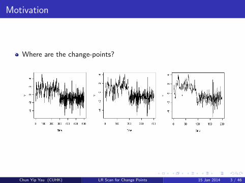
Motivation
Where are the change-points?
Chun Yip Yau (CUHK) LR Scan for Change Points 15 Jan 2014 3 / 46

...
Motivation
Where are the change-points?
Literatures:
|τ − τ0| = Op(1) .
⇒To locate a change-point,
We don’t really need too many data.
Chun Yip Yau (CUHK) LR Scan for Change Points 15 Jan 2014 4 / 46
...
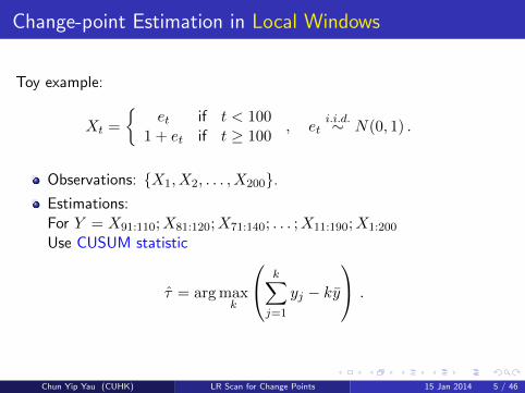
Change-point Estimation in Local Windows
Toy example:
Xt =
et if t < 100
1 + et if t ≥ 100, et
i.i.d.∼ N(0, 1) .
Observations: X1, X2, . . . , X200.Estimations:For Y = X91:110;X81:120;X71:140; . . . ;X11:190;X1:200
Use CUSUM statistic
τ = arg maxk
k∑j=1
yj − ky
.
Chun Yip Yau (CUHK) LR Scan for Change Points 15 Jan 2014 5 / 46

...
Change-point Estimation in Local Windows
0 50 100 150 200
−2−1
01
2
0 50 100 150 200
−20
12
3
0 50 100 150 200
−20
12
3
0 50 100 150 200
−20
12
3
0 50 100 150 200
−20
12
3
0 50 100 150 200
−20
12
3
0 50 100 150 200
−20
12
3
0 50 100 150 200
−20
12
3
0 50 100 150 200
−20
12
3
0 50 100 150 200
−20
12
3
Findings:
In 80/100 replications, the 10 τs are exactly the same.
For the other 20 replications, the average s.d. of the 10 τs is 3.43.
Chun Yip Yau (CUHK) LR Scan for Change Points 15 Jan 2014 6 / 46

...
Main Objectives:
Literatures:
Scan Statistics: Naus (1965), Glaz (2001) . . .
Testing for Change-point: Bauer & Hackl (78, 80), Chan &Walther (13) . . .
Location estimation: Fryzlewicz (14), Dette (14)
Objectives: By using a Likelihood Ratio Scan Statistic,
Consistent estimation of multiple change-points in time series.
Construction of confidence intervals.
Fast and easy to implement
Chun Yip Yau (CUHK) LR Scan for Change Points 15 Jan 2014 7 / 46
...
Content
1 Motivation
2 Likelihood Ratio Scan for Change-Points DetectionChange-point Detection by Scan StatisticConsistent Change-point Estimation by Model SelectionConstruction of Confidence Intervals
3 Implementation Issue and Computational Complexity
4 Simulation Studies
5 Applications
6 Conclusions
Chun Yip Yau (CUHK) LR Scan for Change Points 15 Jan 2014 8 / 46

...
Content
1 Motivation
2 Likelihood Ratio Scan for Change-Points DetectionChange-point Detection by Scan StatisticConsistent Change-point Estimation by Model SelectionConstruction of Confidence Intervals
3 Implementation Issue and Computational Complexity
4 Simulation Studies
5 Applications
6 Conclusions
Chun Yip Yau (CUHK) LR Scan for Change Points 15 Jan 2014 9 / 46

...
Setting and Notations
Data: Piecewise stationary autoregressive time series Xtnt=1
Y
0 100 200 300 400 500 600 700
-4-2
02
46
…
…, , , (1)
(n)The j-th stationary segment: Yt,j , τj−1 < t ≤ τj
Yt,j = φj0 + φj1Yt−1,j + · · ·+ φj,pjYt−pj ,j + σjεt , εti.i.d.∼ N(0, 1) .
Parameters:
Break-points: 0 = τ0, τ1, τ2, ..., τm, τm+1 = nRelative location of breaks: λj :=
τjn . Assume |λj+1 − λj | > ελ.
AR parameter vectors: θj := (φj,0, φj,1, . . . , φj,pj , σ2j ).
Chun Yip Yau (CUHK) LR Scan for Change Points 15 Jan 2014 10 / 46
...
Outline
1 Motivation
2 Likelihood Ratio Scan for Change-Points DetectionChange-point Detection by Scan StatisticConsistent Change-point Estimation by Model SelectionConstruction of Confidence Intervals
3 Implementation Issue and Computational Complexity
4 Simulation Studies
5 Applications
6 Conclusions
Chun Yip Yau (CUHK) LR Scan for Change Points 15 Jan 2014 11 / 46
...
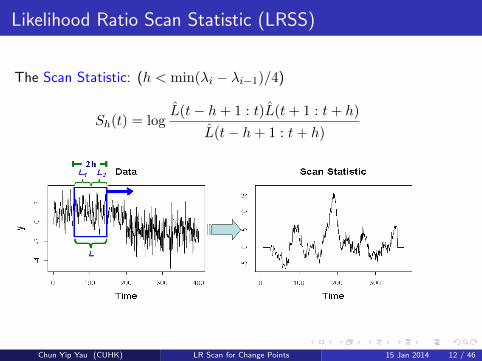
Likelihood Ratio Scan Statistic (LRSS)
The Scan Statistic: (h < min(λi − λi−1)/4)
Sh(t) = logL(t− h+ 1 : t)L(t+ 1 : t+ h)
L(t− h+ 1 : t+ h)
Chun Yip Yau (CUHK) LR Scan for Change Points 15 Jan 2014 12 / 46

...
Likelihood Ratio Scan Statistic (LRSS)
Conditional log-Likelihood of AR model for data y = (y1, . . . , yn):
l(θ,y) = −∑
(yt − φ0 − φ1yt−1 − · · · − φpyt−p)2
2σ2− 1
2log σ2
l(θ,y) = −n2− 1
2log σ2 ,
where σ2 = γ(0)− γT φ, φ = Γ−1γ.
Scan Statistics
Sh(t) = log σ2t −1
2log σ21,t −
1
2log σ22,t .
Chun Yip Yau (CUHK) LR Scan for Change Points 15 Jan 2014 13 / 46
...
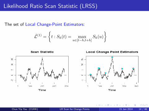
Likelihood Ratio Scan Statistic (LRSS)
The set of Local Change-Point Estimators:
L(1) =
t : Sh(t) = max
u∈[t−h,t+h]Sh(u)
Chun Yip Yau (CUHK) LR Scan for Change Points 15 Jan 2014 14 / 46

...
Likelihood Ratio Scan Statistic (LRSS)
Theorem 1
Let
True CP: Lo = (τ o1 , . . . , τomo)
Local CP estimates: L(1) = τ (1)1 , τ(1)2 , . . . , τ
(1)
m(1)minj=1,...,mo(λ
oj+1 − λoj) > ελ
There exists some d > 0 such that for h ≥ d log n and h < nελ/4,
P
(maxτoj ∈L0
minτ(1)k ∈L(1)
|τ oj − τ(1)k | < h
)→ 1 .
Possibly overestimation: m(1) > mo
Each of the true τ oj is surrounded by a τ(1)k in a h-neighborhood.
Chun Yip Yau (CUHK) LR Scan for Change Points 15 Jan 2014 15 / 46

...
Outline
1 Motivation
2 Likelihood Ratio Scan for Change-Points DetectionChange-point Detection by Scan StatisticConsistent Change-point Estimation by Model SelectionConstruction of Confidence Intervals
3 Implementation Issue and Computational Complexity
4 Simulation Studies
5 Applications
6 Conclusions
Chun Yip Yau (CUHK) LR Scan for Change Points 15 Jan 2014 16 / 46

...
Estimation of Change-points
From the scanning step, we have L(1) = τ (1)1 , τ(1)2 , . . . , τ
(1)m with
P
(maxτoj ∈L0
minτ(1)k ∈L(1)
|τ oj − τ(1)k | < h
)→ 1 .
Infeasible: (m, L, p) = arg minL⊂1,2,...,n
IC(m,L,p)
Feasible: (m(2), L(2), p(2)) = arg minL⊂L(1)
IC(m,L,p)
Examples:
AIC(m,L,p) =m+1∑j=1
nj
2 log(σ2j ) + 2(m+
m+1∑j=1
(pj + 2))
BIC(m,L,p) =m+1∑j=1
nj
2 log(σ2j ) + (m+
m+1∑j=1
(pj + 2)) log n
MDL(m,L,p) =m+1∑j=1
nj
2 log(σ2j ) +
m+1∑j=1
pj+22 log(nj) + (m+ 1) log(n)
Chun Yip Yau (CUHK) LR Scan for Change Points 15 Jan 2014 17 / 46
...
Estimation of Change-points
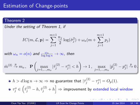
Theorem 2
Under the setting of Theorem 1, if
IC(m,L,p) =
m+1∑j=1
nj2
log(σ2j ) + ωn(m+
m+1∑j=1
pj)
with ωn = o(n) and ωnlog logn →∞, then
m(2) p→ mo , P
(max
j=1,...,mo|τ (2)j − τ
oj | < h
)→ 1 , max
j=1,...,mo|p(2)j − p
oj |
p→ 0 .
h > d log n→∞⇒ no guarantee that |τ (2)j − τ oj | = Op(1).
τ oj ∈(τ(2)j − h, τ
(2)j + h
]⇒ improvement by extended local window
Chun Yip Yau (CUHK) LR Scan for Change Points 15 Jan 2014 18 / 46
...
Outline
1 Motivation
2 Likelihood Ratio Scan for Change-Points DetectionChange-point Detection by Scan StatisticConsistent Change-point Estimation by Model SelectionConstruction of Confidence Intervals
3 Implementation Issue and Computational Complexity
4 Simulation Studies
5 Applications
6 Conclusions
Chun Yip Yau (CUHK) LR Scan for Change Points 15 Jan 2014 19 / 46

...
Final Estimates and Confidence Intervals
From the model selection step we have
P(τ oj ∈
(τ(2)j − h, τ
(2)j + h
])→ 1
Define the extended local window
Ej =(τ(2)j − 2h, τ
(2)j + 2h
]⇒ τ oj is within
(14 ,
34
)of Ej .
Ej contains one τojNumber of observation before/after τoj →∞
⇒ Final estimate and C.I. can be obtained from Ej
Chun Yip Yau (CUHK) LR Scan for Change Points 15 Jan 2014 20 / 46

...
Final estimates and Confidence Intervals
Final Estimates of Change Points
τ(3)j = arg max
τ∈(τ (2)j −h,τ(2)j +h]
logL(τ(2)j − 2h+ 1 : τ)L(τ + 1 : τ
(2)j + 2h)
Theorem 3
Under the setting of Theorem 1 and 2,
maxj=1,...,mo
|τ (3)j − τoj | = Op(1) .
Chun Yip Yau (CUHK) LR Scan for Change Points 15 Jan 2014 21 / 46

...
Final Estimates and Confidence Intervals
Theorem 4
Asymptotic distribution of Change Points (Ling (2013))
τ(3)j − τ
oj
d→ arg maxk
Wk ,
where
Wk =
∑τoj +k
t=τoj(lt(θ
o1)− lt(θo2)) k > 0
0 k = 0∑τoj −1t=τoj +k
(lt(θo2)− lt(θo1)) k < 0
is the double-sided random walk.
Unknown closed form expression for the c.d.f. of Wk.
Chun Yip Yau (CUHK) LR Scan for Change Points 15 Jan 2014 22 / 46
...
Final Estimates and Confidence Intervals
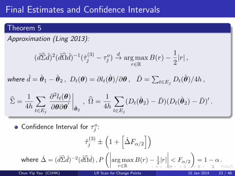
Theorem 5
Approximation (Ling 2013):
(dΣd)2(dΩd)−1(τ(3)j − τ
oj )
d→ arg maxr∈R
B(r)− 1
2|r| ,
where d = θ1 − θ2 , Dt(θ) = ∂lt(θ)/∂θ , D =∑
t∈Ej Dt(θ)/4h ,
Σ =1
4h
∑t∈Ej
∂2lt(θ)
∂θ∂θ′
∣∣∣∣θ2
, Ω =1
4h
∑t∈Ej
(Dt(θ2)− D)(Dt(θ2)− D)′ .
Confidence Interval for τ oj :
τ(3)j ±
(1 +
[∆Fα/2
])where ∆ = (dΣd)−2(dΩd) , P
(∣∣∣∣arg maxr∈R
B(r)− 12 |r|∣∣∣∣ < Fα/2
)= 1− α .
Chun Yip Yau (CUHK) LR Scan for Change Points 15 Jan 2014 23 / 46
...
Content
1 Motivation
2 Likelihood Ratio Scan for Change-Points DetectionChange-point Detection by Scan StatisticConsistent Change-point Estimation by Model SelectionConstruction of Confidence Intervals
3 Implementation Issue and Computational Complexity
4 Simulation Studies
5 Applications
6 Conclusions
Chun Yip Yau (CUHK) LR Scan for Change Points 15 Jan 2014 24 / 46
...
Three-step procedure for change-point estimation
Summary
Step 1: Detection by Likelihood Ratio Scan Statistics.
Step 2: Model Selection by Information Criterion.
Step 3: Construction of Confidence Intervals.
Chun Yip Yau (CUHK) LR Scan for Change Points 15 Jan 2014 25 / 46
...
Three-step procedure for change-point estimation
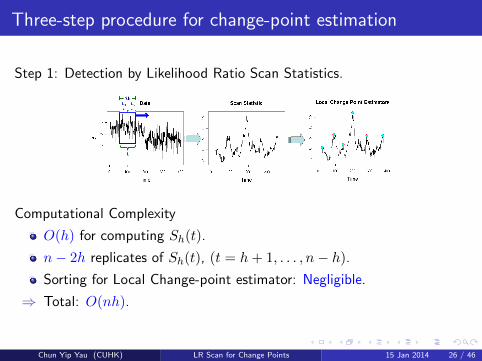
Step 1: Detection by Likelihood Ratio Scan Statistics.
Computational Complexity
O(h) for computing Sh(t).
n− 2h replicates of Sh(t), (t = h+ 1, . . . , n− h).
Sorting for Local Change-point estimator: Negligible.
⇒ Total: O(nh).
Chun Yip Yau (CUHK) LR Scan for Change Points 15 Jan 2014 26 / 46
...
Three-step procedure for change-point estimation
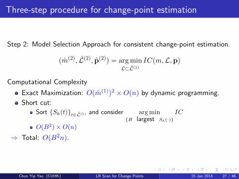
Step 2: Model Selection Approach for consistent change-point estimation.
(m(2), L(2), p(2)) = arg minL⊂L(1)
IC(m,L,p)
Computational Complexity
Exact Maximization: O(m(1))2 ×O(n) by dynamic programming.
Short cut:
Sort Sh(t)t∈L(1) and consider arg minB largest Sh(·)
IC
O(B2)×O(n)
⇒ Total: O(B2n).
Chun Yip Yau (CUHK) LR Scan for Change Points 15 Jan 2014 27 / 46
...
Three-step procedure for change-point estimation
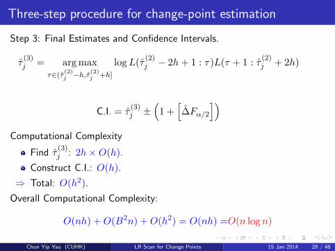
Step 3: Final Estimates and Confidence Intervals.
τ(3)j = arg max
τ∈(τ (2)j −h,τ(2)j +h]
logL(τ(2)j − 2h+ 1 : τ)L(τ + 1 : τ
(2)j + 2h)
C.I. = τ(3)j ±
(1 +
[∆Fα/2
])Computational Complexity
Find τ(3)j : 2h×O(h).
Construct C.I.: O(h).
⇒ Total: O(h2).
Overall Computational Complexity:
O(nh) +O(B2n) +O(h2) = O(nh) =O(n log n)
Chun Yip Yau (CUHK) LR Scan for Change Points 15 Jan 2014 28 / 46
...
Content
1 Motivation
2 Likelihood Ratio Scan for Change-Points DetectionChange-point Detection by Scan StatisticConsistent Change-point Estimation by Model SelectionConstruction of Confidence Intervals
3 Implementation Issue and Computational Complexity
4 Simulation Studies
5 Applications
6 Conclusions
Chun Yip Yau (CUHK) LR Scan for Change Points 15 Jan 2014 29 / 46
...
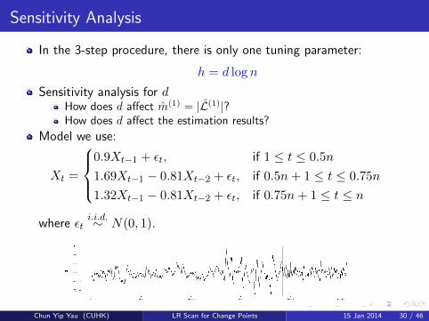
Sensitivity Analysis
In the 3-step procedure, there is only one tuning parameter:
h = d log n
Sensitivity analysis for dHow does d affect m(1) = |L(1)|?How does d affect the estimation results?
Model we use:
Xt =
0.9Xt−1 + εt, if 1 ≤ t ≤ 0.5n
1.69Xt−1 − 0.81Xt−2 + εt, if 0.5n+ 1 ≤ t ≤ 0.75n
1.32Xt−1 − 0.81Xt−2 + εt, if 0.75n+ 1 ≤ t ≤ n
where εti.i.d.∼ N(0, 1).
Chun Yip Yau (CUHK) LR Scan for Change Points 15 Jan 2014 30 / 46
...
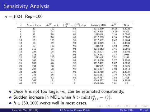
Sensitivity Analysis
n = 1024, Rep=100
d h = d logn m(2) = 2 |τ(2)j − τ(o)j | < h Average MDL m(1) Time
2 13 100 54 1011.139 34.95 8.37254 27 98 80 1013.365 17.65 4.2676 41 98 85 1015.85 11.4 3.05478 55 98 92 1017.205 8.39 2.690510 69 100 91 1017.182 6.42 2.576412 83 99 93 1018.079 5 2.430514 97 100 99 1016.94 3.93 2.28616 110 98 96 1015.052 3.41 2.266518 124 98 98 1015.527 2.88 2.130620 138 100 98 1015.273 2.73 2.05622 152 100 99 1013.48 2.51 2.11124 166 99 99 1013.638 2.27 1.988226 180 98 98 1012.462 2.07 1.805828 194 98 98 1012.07 1.99 1.822530 207 98 98 1011.397 1.98 1.851832 221 91 91 1012.718 1.91 1.612734 235 76 76 1020.511 1.76 1.722836 249 52 52 1029.787 1.52 1.80538 263 3 3 1049.257 1.03 1.358240 277 1 1 1049.649 1.01 1.3
Once h is not too large, mo can be estimated consistently.
Sudden increase in MDL when h > min(τ oj+1 − τ oj ).
h ∈ (50, 100) works well in most cases.
Chun Yip Yau (CUHK) LR Scan for Change Points 15 Jan 2014 31 / 46
...
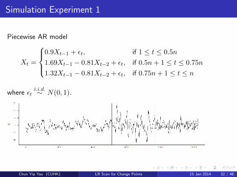
Simulation Experiment 1
Piecewise AR model
Xt =
0.9Xt−1 + εt, if 1 ≤ t ≤ 0.5n
1.69Xt−1 − 0.81Xt−2 + εt, if 0.5n+ 1 ≤ t ≤ 0.75n
1.32Xt−1 − 0.81Xt−2 + εt, if 0.75n+ 1 ≤ t ≤ n
where εti.i.d.∼ N(0, 1).
Chun Yip Yau (CUHK) LR Scan for Change Points 15 Jan 2014 32 / 46
...
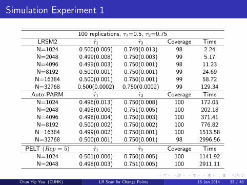
Simulation Experiment 1
100 replications, τ1=0.5, τ2=0.75
LRSM2 τ1 τ2 Coverage Time
N=1024 0.500(0.009) 0.749(0.013) 98 2.24N=2048 0.499(0.008) 0.750(0.003) 99 5.17N=4096 0.499(0.003) 0.750(0.001) 98 11.23N=8192 0.500(0.001) 0.750(0.001) 99 24.69N=16384 0.500(0.001) 0.750(0.001) 99 58.72N=32768 0.500(0.0002) 0.750(0.0002) 99 129.34
Auto-PARM τ1 τ2 Coverage Time
N=1024 0.496(0.013) 0.750(0.008) 100 172.05N=2048 0.498(0.006) 0.751(0.005) 100 202.18N=4096 0.498(0.004) 0.750(0.003) 100 371.41N=8192 0.500(0.002) 0.750(0.002) 100 776.82N=16384 0.499(0.002) 0.750(0.001) 100 1513.58N=32768 0.500(0.001) 0.750(0.001) 98 2996.56
PELT (Rep = 5) τ1 τ2 Coverage Time
N=1024 0.501(0.006) 0.750(0.005) 100 1141.92N=2048 0.498(0.003) 0.751(0.005) 100 2911.11
Chun Yip Yau (CUHK) LR Scan for Change Points 15 Jan 2014 33 / 46
...
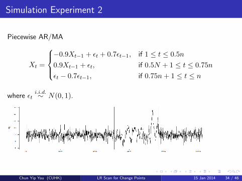
Simulation Experiment 2
Piecewise AR/MA
Xt =
−0.9Xt−1 + εt + 0.7εt−1, if 1 ≤ t ≤ 0.5n
0.9Xt−1 + εt, if 0.5N + 1 ≤ t ≤ 0.75n
εt − 0.7εt−1, if 0.75n+ 1 ≤ t ≤ n
where εti.i.d.∼ N(0, 1).
Chun Yip Yau (CUHK) LR Scan for Change Points 15 Jan 2014 34 / 46
...
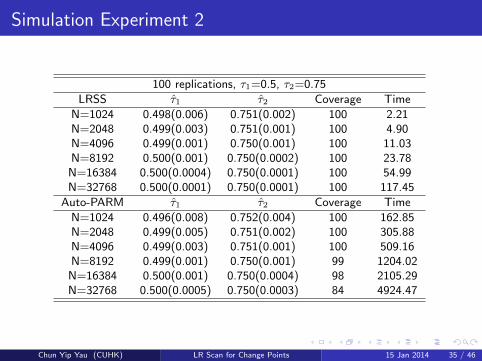
Simulation Experiment 2
100 replications, τ1=0.5, τ2=0.75
LRSS τ1 τ2 Coverage Time
N=1024 0.498(0.006) 0.751(0.002) 100 2.21N=2048 0.499(0.003) 0.751(0.001) 100 4.90N=4096 0.499(0.001) 0.750(0.001) 100 11.03N=8192 0.500(0.001) 0.750(0.0002) 100 23.78N=16384 0.500(0.0004) 0.750(0.0001) 100 54.99N=32768 0.500(0.0001) 0.750(0.0001) 100 117.45
Auto-PARM τ1 τ2 Coverage Time
N=1024 0.496(0.008) 0.752(0.004) 100 162.85N=2048 0.499(0.005) 0.751(0.002) 100 305.88N=4096 0.499(0.003) 0.751(0.001) 100 509.16N=8192 0.499(0.001) 0.750(0.001) 99 1204.02N=16384 0.500(0.001) 0.750(0.0004) 98 2105.29N=32768 0.500(0.0005) 0.750(0.0003) 84 4924.47
Chun Yip Yau (CUHK) LR Scan for Change Points 15 Jan 2014 35 / 46
...
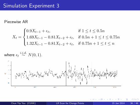
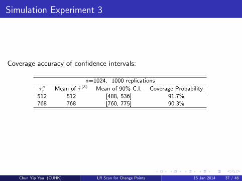
Simulation Experiment 3
Piecewise AR
Xt =
0.9Xt−1 + εt, if 1 ≤ t ≤ 0.5n
1.69Xt−1 − 0.81Xt−2 + εt, if 0.5n+ 1 ≤ t ≤ 0.75n
1.32Xt−1 − 0.81Xt−2 + εt, if 0.75n+ 1 ≤ t ≤ n
where εti.i.d.∼ N(0, 1).
Chun Yip Yau (CUHK) LR Scan for Change Points 15 Jan 2014 36 / 46
...
Simulation Experiment 3
Coverage accuracy of confidence intervals:
n=1024, 1000 replications
τoj Mean of τ (3) Mean of 90% C.I. Coverage Probability
512 512 [488, 536] 91.7%768 768 [760, 775] 90.3%
Chun Yip Yau (CUHK) LR Scan for Change Points 15 Jan 2014 37 / 46

...
Content
1 Motivation
2 Likelihood Ratio Scan for Change-Points DetectionChange-point Detection by Scan StatisticConsistent Change-point Estimation by Model SelectionConstruction of Confidence Intervals
3 Implementation Issue and Computational Complexity
4 Simulation Studies
5 Applications
6 Conclusions
Chun Yip Yau (CUHK) LR Scan for Change Points 15 Jan 2014 38 / 46

...
Electroencephalogram (EEG) Time Series
Recorded from a patient diagnosed with left temporal lobe epilepsy.
Data collection:
Sampling rate: 100Hz,Recording period: 5 minutes and 28 seconds,Sample size: n=32,768.
Investigated by Ombao et al. (2000) and Davis, Lee andRodriguez-Yam (2006).
Chun Yip Yau (CUHK) LR Scan for Change Points 15 Jan 2014 39 / 46
...
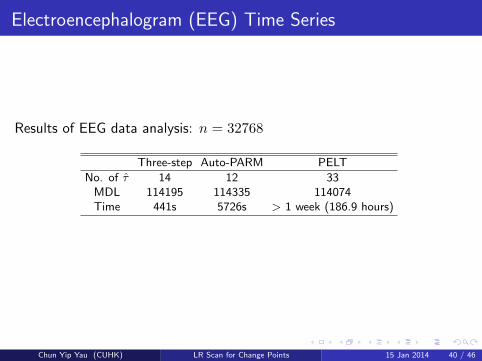
Electroencephalogram (EEG) Time Series
Results of EEG data analysis: n = 32768
Three-step Auto-PARM PELT
No. of τ 14 12 33MDL 114195 114335 114074Time 441s 5726s > 1 week (186.9 hours)
Chun Yip Yau (CUHK) LR Scan for Change Points 15 Jan 2014 40 / 46
...
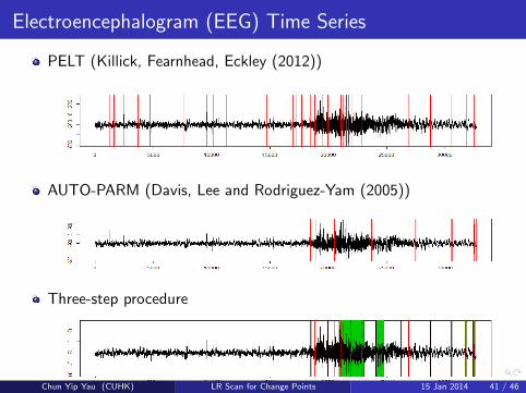
Electroencephalogram (EEG) Time Series
PELT (Killick, Fearnhead, Eckley (2012))
AUTO-PARM (Davis, Lee and Rodriguez-Yam (2005))
Three-step procedure
Chun Yip Yau (CUHK) LR Scan for Change Points 15 Jan 2014 41 / 46

...
IBM return data
From Jan 1926 to Dec 2008.
996 data points.
Time for computation: 4.2s
Chun Yip Yau (CUHK) LR Scan for Change Points 15 Jan 2014 42 / 46
...
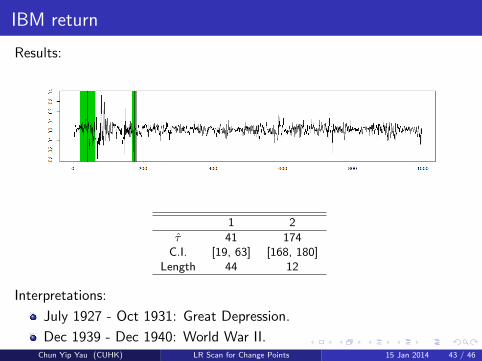
IBM return
Results:
1 2
τ 41 174C.I. [19, 63] [168, 180]
Length 44 12
Interpretations:
July 1927 - Oct 1931: Great Depression.
Dec 1939 - Dec 1940: World War II.Chun Yip Yau (CUHK) LR Scan for Change Points 15 Jan 2014 43 / 46
...
Content
1 Motivation
2 Likelihood Ratio Scan for Change-Points DetectionChange-point Detection by Scan StatisticConsistent Change-point Estimation by Model SelectionConstruction of Confidence Intervals
3 Implementation Issue and Computational Complexity
4 Simulation Studies
5 Applications
6 Conclusions
Chun Yip Yau (CUHK) LR Scan for Change Points 15 Jan 2014 44 / 46
...
Conclusions
Fast three-step procedure for change-points inference.
Step 1: Detection using Scan statisticsStep 2: Estimation by model selection information criterion.Step 3: Extended window for CI
Advantages:
FastFew and non-sensitive tuning parametersEspecially suitable for large n small m case.
Chun Yip Yau (CUHK) LR Scan for Change Points 15 Jan 2014 45 / 46

...
Thank You!
Chun Yip Yau (CUHK) LR Scan for Change Points 15 Jan 2014 46 / 46