inference about the ratio of means from negative binomial paired count data

Environ Ecol Stat (2012) 19:269–293DOI 10.1007/s10651-011-0186-8

Inference about the ratio of means from NegativeBinomial paired count data

N. G. Cadigan · O. M. Bataineh

Received: 13 July 2010 / Revised: 25 November 2011 / Published online: 25 December 2011© Her Majesty the Queen in Right of Canada 2011

Abstract We derive some statistical properties of the distribution of two NegativeBinomial random variables conditional on their total. This type of model can be appro-priate for paired count data with Poisson over-dispersion such that the variance is aquadratic function of the mean. This statistical model is appropriate in many ecolog-ical applications including comparative fishing studies of two vessels and or gears.The parameter of interest is the ratio of pair means. We show that the conditionalmeans and variances are different from the more commonly used Binomial modelwith variance adjusted for over-dispersion, or the Beta-Binomial model. The condi-tional Negative Binomial model is complicated because it does not eliminate nuisanceparameters like in the Poisson case. Maximum likelihood estimation with the uncon-ditional Negative Binomial model can result in biased estimates of the over-dispersionparameter and poor confidence intervals for the ratio of means when there are manynuisance parameters. We propose three approaches to deal with nuisance parametersin the conditional Negative Binomial model. We also study a random effects Binomialmodel for this type of data, and we develop an adjustment to the full-sample Neg-ative Binomial profile likelihood to reduce the bias caused by nuisance parameters.We use simulations with these methods to examine bias, precision, and accuracy of

N. G. Cadigan (B)Science Branch, Fisheries and Oceans Canada, St. John’s, NL A1C 5X1, Canadae-mail: [email protected]

O. M. BatainehDepartment of Mathematics and Statistics, Memorial University,St. John’s, NL A1C 5S7, Canada

Present Address:O. M. BatainehDepartment of Mathematics and Statistics, University of Saskatchewan,Saskatoon, SK, S7N 5E6, Canada

123

270 Environ Ecol Stat (2012) 19:269–293

estimators and confidence intervals. We conclude that the maximum likelihood methodbased on the full-sample Negative Binomial adjusted profile likelihood produces thebest statistical inferences for the ratio of means when paired counts have NegativeBinomial distributions. However, when there is uncertainty about the type of Poissonover-dispersion then a Binomial random effects model is a good choice.

Keywords Conditional distribution · Negative Binomial · Profile likelihood ·Random effects · Adjusted profile likelihood · Confidence interval

1 Introduction

There are many experimental and observational studies in ecological and other disci-plines (e.g. Martinsen et al. 1998; Lowry 1999; Teunis et al. 1999; Schreibman andFriedland 2004; Middlemas et al. 2009) that generate paired count data to be used forinference about population parameters. The data consist of a set of H pairs of countobservations {(Y11,Y12), . . . , (YH1,YH2)} from two treatments, conditions, etc. Eachpair could also have covariates associated with it. We assume the pairs are independentwith means

E(Yhi ) = τiλh, (1)

where τi is the treatment effect (i = 1, 2) andλh is the pair effect, h = 1, . . . , H . Oftenthe interest is in the size of one treatment effect compared to the other, ρ = τ1/τ2. Letμhi = E(Yhi ). These means are linearly related,

μh1 = ρμh2, h = 1, . . . , H. (2)

Let μh· = μh1 + μh2, p = ρ/(1 + ρ) and q = 1 − p. Equation (2) is equivalent to

μh1 = pμh·, μh2 = qμh·, h = 1, . . . , H. (3)

This is a common model used for paired count data (e.g. Lee 1996). The main objec-tive is to estimate p (or ρ ) and confidence intervals (CI’s) for p (or ρ). The μh·’s areassumed to be nuisance parameters that are of no direct relevance. Each pair can bethought of as two observations from a strata, and μh· is a stratum-specific parameter.A highly stratified experiment or survey design refers to the situation where there aremany strata with few observations per strata. Therefore, model (3) is highly stratified.

We are particularly interested in fish catch data from paired fishing experiments inwhich two nets are towed close together at fixed speeds and distances. This type ofdata is produced in gear size-selectivity studies (e.g. Millar 1992; Dahm et al. 2002)or fish stock survey calibration studies (e.g. Pelletier 1998; Lewy et al. 2004) whichwe refer to collectively as comparative fishing studies. They generate paired countsof fish catches for two types of fishing activities (e.g. gears and/or vessels 1 and 2).Because the trawls are fished close together it is reasonable to assume that each trawlencounters the same density of fish (i.e. λh in Eq. 1) and differences in catches are

123

Environ Ecol Stat (2012) 19:269–293 271

primarily related to differences in gear selectivity or vessel fishing efficiency (i.e. τ1and τ2 in Eq. 1). The parameter of interest is the ratio, ρ = τ1/τ2. Note that ρ coulddepend on factors such as length, towing speed, or depth. We do not consider sucheffects in this paper but our methods can be extended to the regression setting in astraight-forward manner.

If the counts are Poisson distributed then a good approach (see Section 4.5 in Coxand Snell 1989, and Example 3.1 in Reid 1995) for inferences about p (or ρ) is to con-dition on the observed values of Yh1 +Yh2 = Yh·, h = 1, . . . , H. It is well known thatYh· is a complete sufficient statistic for μh· and in the absence of further informationabout μh1 and μh2, Yh· provides no information about p. In this case, the conditionaldistribution Yh1|Yh· provides all the sample information about p. Yh1|Yh· has a Bino-mial distribution with E(Yh1|Yh· = th) = th p. The distribution of the H conditionalobservations involves only one unknown parameter p which can be easily estimatedusing maximum likelihood. Basing inferences about p on the conditional distributioncan also be motivated from a hypothesis testing framework (see Reid 1995).

A problem with the above approach is that in many situations the Poisson assump-tion is not reasonable. Poisson overdispersion is common in count data, especiallyfrom ecological field studies. The Negative Binomial (NB) distribution is often usedto model count data with Poisson-overdispersion, including catches from surveys offish stocks (e.g. Gunderson 1984). Cadigan (2011) showed using analyses of devianceresiduals that NB variability was appropriate for 6 species caught in bottom trawlsurveys off the east coast of Canada, whereas Poisson variability was not appropriate.

We use the Poisson-Gamma mixture formulation of the NB distribution. Instead of(1), we assume that

E(Yhi |λhi ) = τiλhi = τiλhγhi (4)

and γhi is a Gamma random effect with mean 1 and variance k−1. The random stratumeffect λhi in (4) is different for each treatment i but both effects come from a commondistribution. In this case the marginal distribution of Yhi is NB,

Pr(Yhi = y) = �(y + k)

�(k)�(y + 1)

(μhi

k + μhi

)y (k

k + μhi

)k

, (5)

with E(Yhi ) = μhi and V ar(Yhi ) = μhi + μ2hi/k. k is sometimes referred to as the

Poisson overdispersion parameter. When μhi is large then V ar(Yhi ) ∝ μ2hi , but when

μhi is small then V ar(Yhi ).= μhi . Yhi has a Poisson distribution as k → ∞ (e.g.

Cameron and Trivedi 1998).When the number of nuisance parameters is large it is well known that mle’s for

some parameters, particularly for variances, can be badly biased and inconsistent(e.g. Section 4.3 in Barndorff-Nielsen and Cox 1994). In the highly stratified setting,Sartori (2003) and Bellio and Sartori (2006) showed that standard likelihood infer-ences may not be accurate. In a simulation study, Bellio and Sartori (2006) found thatthe mle relative bias for k was over 50% for a highly parameterized NB model.Allison and Waterman (2002) reported a similar problem. This can lead to very

123


inaccurate CI’s for parameters like p. Finding a conditional distribution that doesnot depend on nuisance parameters is one approach to deal with this problem.

When paired counts are NB distributed then the conditional distribution is no longerBinomial and is rather complicated because it still depends on theμh· nuisance param-eters in addition to p and k. The separation of information about p and μh·’s does notoccur like in the Poisson case. This is because there is no complete sufficient statisticsforμh· that is a function of the data alone (see Allison and Waterman 2002). However,if the conditional NB distribution, which we refer to as the NBc distribution, is onlyweakly sensitive to theμh·’s then more reliable inferences about p may be obtained bysubstituting estimates of μh·’s obtained from the marginal distribution of pair-totals.The first step is to better understand the statistical properties of the NBc distribution,and how they are affected by μh·, which is the subject of Sect. 2.

Other approaches are possible. A common way to deal with over-dispersed Bino-mial data is to use quasi-likelihood (e.g. McCullagh and Nelder 1989) with the variancemodel V ar(Yh1|Yh· = th) = φth pq. Solís-Trápala and Farewell (2005) and Hausmanet al. (1984) considered different types of NB distributions in which V ar(Y ) = φμ.Cameron and Trivedi (1998) referred to this as the NB1 model, and they referred tothe more common formulation in (5) as the NB2 model. In Hausman et al. (1984)the conditional distribution is free of nuisance parameters, but in Solís-Trápala andFarewell (2005) it is not. However, this variance model may not be appropriate fortrawl catches (Cadigan 2011). Lee (1996) used a version of the NB model in whichthe same Gamma mixing random variable (rv) γ affected both Yh1 and Yh2. Allisonand Waterman (2002) also considered this approach. The resulting loglikelihood isproportional to the Binomial, and the mle of p and its variance are identical to theBinomial result. However, we do not expect γ to be the for each gear in compara-tive fishing studies, so this model does not seem appropriate. Cadigan and Dowden(2010) used a Binomial Generalized Linear Mixed Model (GLMM; e.g. McCullochand Searle 2001) for inferences about ρ. This was based on a normal approximationfor the log ratio of the Gamma random effects in (4). The Beta-Binomial model waspreferred by Miller et al. (2010) for vessel calibration data when H > 30. Over-dis-persion is accounted for by assuming the between-strata distribution in ph’s is Beta.Various likelihood adjustments have also been proposed to correct for the bias in mle’sresulting from nuisance parameters and many of these are reviewed by Severini (2000)and Cox (2006). The adjusted likelihood lM in Severini (2000; Section 9.5.4) is con-venient for discrete distributions like the NB (e.g. Bellio and Sartori 2006) and wealso investigate this approach.

The estimators of p we consider are (1) Binomial mle with standard errors adjustedfor overdispersion (BINOD), (2) unconditional full-sample NB mle (NBF), (3) full-sample lM -adjusted NB mle (ANBF), (4) Binomial GLMM with a random intercept(BINRI), (5–6) two mle’s based on the NBc distribution (NBct, NBc1), and (7) theBeta-Binomial mle (BETABIN). First, some basic statistical properties of the NBc dis-tribution are presented in Sect. 2. The NBF, ANBF, and NBc mle’s are developed inSect. 3 and illustrated in Sect. 4 using two case studies. In Sect. 5 we use simulations tocompare the bias, efficiency, and confidence interval coverage of these various meth-ods for practical sample sizes and other data characteristics. A discussion in presentedin Sect. 6.

123


2 Conditional distribution of two Negative Binomial random variables

Let Y1 and Y2 be NB rv’s with means μi and variances μi (1 + μi/k), i = 1, 2.Let Y· = Y1 + Y2, μ· = μ1 + μ2, and define p = μ1/μ· and q = 1 − p. It isstraight-forward to show that

Pr(Y1 = y|Y· = t) =�(k+y)�(k+t−y)�(y+1)�(t−y+1)

(pq

)y (qμ·+kpμ·+k

)y

∑tx=0

�(k+x)�(k+t−x)�(x+1)�(t−x+1)

(pq

)x (qμ·+kpμ·+k

)x . (6)

We refer to this as the NBc distribution. A computational algorithm is given in Sect. 7.1.However, simple expressions for moments do not exist in general.

When p = q = 1/2 then (6) has a more simple form. It is a symmetric discretedistribution on 0, . . . , t with moments

Ec(Y1; p = 1/2) = t

2, and V arc(Y1; p = 1/2) = t (2k + t)

4(2k + 1). (7)

The variance is developed in Sect. 7.2. The mean is the same as the Binomial result,but the variance is inflated by the factor

V I F(t, k) = (2k + t)

(2k + 1).

Clearly limk→∞ V I F(t, k) = 1 which makes sense because the NB distribution isPoisson as k → ∞. Also, V I F(1, k) = 1 which suggests that NB over-dispersiondoes not affect binary data, but limt→∞ V I F(t, k) = ∞ and NB over-dispersion willbe important when t is large. The conditional variance is similar to the Beta-Binomialvariance tpq{1 + (t − 1)ψ} (see p. 140 in McCullagh and Nelder 1989) for p = 1/2and ψ = (2k + 1)−1.

The NBc conditional moments equal (7) as μ· = E(Y.) → ∞ for all p ∈ (0, 1).This suggests that the data are less informative about ρ = p/q when μ· is large. Thisis very different from the Binomial result. The same result holds for Ec(Y1) whenk → 0, in which case the NB variance inflation factor is V I F(t, k) = t . We comparethe NBc and Binomial means in Fig. 1 to investigate how the mean is affected by k andby differences in μ· and t . We plotted the expectations in terms of percent differencewith t/2,

percent difference = 100

(Ec(Y1)− t/2

t/2

),

so that if Ec(Y1) = tp then the percent difference is 100(2p − 1) and if Ec(Y1) = t/2then the percent difference is zero. This indicates the range of information about p;that is, the conditional mean is directly informative about p when Ec(Y1) = tp and themean is uninformative about p when Ec(Y1) = t/2. A grey solid line at 100(2p − 1)versus p is shown for reference in Fig. 1. The values of k = 0.1 and k = 10 may not be

123


−80−40

04080 k=0.1

k=1k=10

t = 5 t = 25

0.1

t = 50

−80−40

04080

0.5

−80−40

04080

1

−80−40

04080

2

0.25 0.50 0.75

−80−40

04080

0.25 0.50 0.75 0.25 0.50 0.75

10

p

Per

cent

Diff

eren

ce

Fig. 1 Percent difference in the NBc expectation and t/2. Each line type corresponds to a different valuefor k. Each panel corresponds to different values of t (shown at top) and μ·/t (shown at right). The greyreference line shows the Binomial result

practically relevant but are shown to illustrate the properties of Ec(Y1). We illustratedthe moments in terms of μ·/t = 0.1, 0.5, 1, 2, and 10. If μ· = t then Ec(Y1)

.= tpwhen k = 10 but was biased towards t/2 for smaller values of k. The bias was worsefor μ· = 2t , and when μ· = 10t then Ec(Y1)

.= t/2 for all values of k and p. Ec(Y1)

was different from either tp or t/2 when μ· � t .These results suggest that the NBc distribution is sensitive to the μh· nuisance

parameters; hence, this distribution is not directly useful for inferences about p and k.If the NB overdispersion, φNB(μi ) = V ar(Yi )/μi = 1 + μi/k, increases for i = 1or 2 then the information content for p in the conditional distribution is reduced.If φNB(μi ) is very large then the conditional distribution becomes uninformativeabout p. This is similar to the bias attenuation problem in linear regression withcovariate measurement error. However, it may be possible to produce improved esti-mates of p and k by substituting an estimator for μh·, and we propose two options inSect. 3.2.

123


3 Estimation and confidence intervals for p

It is more convenient to estimate β = log(ρ) = log(p/q). This is because β ∈(−∞,∞) and boundary constraints in estimation are not an issue for β, whereas theyare when estimating ρ or p. We also derive CI’s for ρ or p by transforming CI’s for β.

3.1 Full likelihood

We denote the likelihood of the parameters p, k and μ1·, . . . , μH · based on thefull set of H pairs of counts {(y11, y12), . . . , (yH1, yH2)} as l(p, k, {μh·}H

h=1). Letμh·(p, k) denote the mle of μh· for fixed values of p and k. We show in Sect. 7.4that μh·(p, k) is the root of a quadratic equation (i.e. Eq. 12) that is easily solved.Hence, the mle’s of β = log(p/q) and k can be obtained more simply by maximizingl(p, k, {μh·(p, k)}H

h=1). We used the nlminb function in the R software package (R2011) for this. We approximated the standard errors for these mle’s using the inverseof the observed information matrix (see Sect. 7.4). For simplicity we used the standardCI method,

C I (1 − 2α) = β ± Z1−αSE(β). (8)

However, we will show using simulations (see Sect. 5) that these CI’s have poor cov-erage properties, and the problem is related to a large positive bias in the mle for kthat leads to an underestimate of SE(β).

The adjusted likelihood lM proposed by Severini (2000) is developed in Sect. 7.5for model (3). The adjustment factor (i.e. Eq. 14) is added to the profile likelihoodto produce less biased estimates of β and, in particular, k. We use the Hessian of themaximized adjusted likelihood for standard errors (see Sartori 2003).

3.2 Conditional likelihood

We investigate two options for inferences about p and k based on the NBc distribution.The first is to replaceμh· with th in (6) and estimate p and k by maximizing the condi-tional likelihood based on (5). However, the results in Fig. 1 show that the conditionaldistribution is sensitive to errors in approximating μh· with th . In the second optionwe replace μh· by its approximate marginal mle (see Sect. 7.6). For both options weuse the inverse Hessian standard error based on the conditional likelihood.

A closed form expression to the marginal mle of μh· does not exist. We used afirst-order Taylors series approximation to produce a closed form estimator to sim-plify the estimation of p and k using the conditional likelihood. This estimator isthe root of a quadratic estimating equation (Eq. 16 in Sect. 7.6). Bataineh (2008)showed (see his Figures D.11–D.13) that the first order approximation was usuallyvery close to the marginal mle, and that the marginal mle could be very different fromth . Bataineh (2008) also developed a second order approximation mle which is theroot of a somewhat complicated cubic estimating equation that we do not present here.He showed that the second order approximation was slightly closer to the mle than

123


the first order approximation, although the differences were very small unless both kand min(p, 1 − p) were small.

3.3 Offsets

A complication that occurs in practise, including our case studies, is that there aresometimes variations in the size of sampling units that generate the paired counts. It isimportant to account for such variations; failure to do so can be a source of over-disper-sion and lead to biased and/or less precise parameter estimates. Let dhi be the size ofthe i’th unit in stratum h. Equation (1) can be modified to deal with this complication,

E(Yhi ) = τiλhdhi .

It is not difficult to show that the corresponding modification to (3) is

μh1 = phμh·, μh2 = qhμh·,

where

ph = ρ exp(zh)

1 + ρ exp(zh)and zh = log

(dh1

dh2

).

The zh term is often referred to as an offset in GLM’s. We used the R function glmin the stats package (R 2011) for Binomial regression and the R package glmmML(Broström and Holmberg 2011) for mixed Binomial regression, and both proceduresinclude offsets. We also included offsets in R functions we developed for the variousNB methods.

4 Examples

4.1 Reoviruses

We first illustrate methods using paired counts of reoviruses detected in water beforeand after treatment. Ten trials (Table 7 in Teunis et al. 1999) were conducted withthe objective of estimating the ratio of the means. The volumes of water examinedentering and leaving the treatment plant were different, and this can be accountedfor using the offsets described in Sect. 3.3. Estimates of β = log(ρ) are shown inTable 1. Clearly the treatment was effective because ρ

.= 2% indicating that 98% ofthe reoviruses were removed. To illustrate potential differences in inferences usingthe various methods, we computed p-values (see Table 1) for the hypothesis test thatρ = 3%. The p-values were obtained by subtracting log(0.03) from the offsets. If 3%was a target, and the null hypothesis, then we would conclude there was no evidenceto reject the null based on the BETABIN method, and strong evidence based on theNBF method. The other methods indicated weak evidence against the null hypothesis.

123


Table 1 Model results for the reoviruse example

Method β SE(β) ρ p-value∗ OD SE OD

BINOD −3.89 0.20 0.021 0.06 22.01 –BINRI −3.89 0.22 0.020 0.07 0.65 0.17

BETABIN −3.60 0.16 0.028 0.57 0.05 0.02

NBct −3.82 0.20 0.022 0.12 4.41 2.17

NBc1 −3.83 0.21 0.022 0.12 4.39 2.16

NBF −3.90 0.14 0.020 0.01 12.51 5.21

ANBF −3.89 0.22 0.020 0.07 5.12 2.40

β = log(ρ) = logi t (p). The methods are: BINOD binomial logistic regression with an overdispersionparameter, BINRI binomial logistic regression mixed model with a random strata effect, BETABIN Beta-Binomial logistic regression model, NBct conditional NB mle with μh· = th , NBc1 conditional NB mlewith the first order approximate marginal mle for μh·, NBF full sample NB mle, ANBF adjusted fullsample NB mle. SE denotes standard error. The overdispersion (OD) parameters are φ in V ar(Y ) = φtpqfor the BINOD model, the random effects standard deviation (σ ) for the BINRI model, the Beta-Binomialcorrelation parameter, and the NB k parameter for the other methods∗ The p-value is for the test that ρ = 3%

The BINOD estimate of ρ was identical to four decimal places to the value in Teuniset al. (1999). The BETABIN value was different because Teunis et al. (1999) treatedthe nuisance parameters differently.

4.2 Witch flounder

This data came from a comparative fishing study of two survey vessels that were basi-cally ‘sister’ ships. Both vessels used the same survey gear and other survey protocols.Hence, a priori we did not expect any differences in catchability between the two ves-sels; that is, we expected p = 0.5 or ρ = 1. The comparative fishing experimentswere described in Cadigan et al. (2006). Many species are caught in such surveys, andwe focus on witch flounder ( Glyptocephalus cynoglossus) in this example.

There were 57 paired-tows with some catch of witch flounder (see Fig. 2). Fordisplay purposes only, the results in this figure were adjusted for subsampling andtow distances, but we used unadjusted catches and offsets to estimate parameters.There is some evidence that the catchability of the survey vessel Alfred Needler (AN)was greater than the catchability of the survey vessel Wilfred Templeman (WT). Forexample, the AN caught more fish in 68% of the tows. However, Cadigan et al. (2006)concluded that ρ was not significantly different from one based on the BINRI model,although results from the BINOD model did indicate a significant difference at the5% level. These data were further analyzed by Cadigan and Dowden (2010) using twoapproaches for estimating the BINRI model. They also concluded that ρ = 1.

The BINOD (Table 2) estimate of β = log(ρ) = log (p/q) was substantially dif-ferent than the BINRI or the various NB estimates. The BETABIN estimate was alsosomewhat different than the others. As expected the NBF estimate of k was muchlarger than the other NB estimates. This led to the smaller standard error for β andthe small p-value, whereas the other NB estimates had larger p-values. Estimates andstandard errors for β and k were similar for the NBct, NBc1 and the ANBF methods.

123


0 50 100 150 200 250

0

50

100

150

AN (No. per tow)

WT

(N

o. p

er to

w)

Fig. 2 Wilfred Templeman (WT) catch of witch flounder (Glyptocephalus cynoglossus) versus the AlfredNeedler (AN) catch. The grey dashed line is a 1–1 reference line. The Binomial logistic regression estimateof relative efficiency (ρ) is plotted as a dotted line, and the adjusted NB mle is plotted as a black line

Table 2 Model results for the witch flounder (Glyptocephalus cynoglossus) example

Method β SE(β) ρ p-value OD SE OD

BINOD −0.160 0.067 0.852 0.02 5.44 –

BINRI −0.104 0.092 0.901 0.26 0.54 0.08

BETABIN −0.077 0.111 0.926 0.49 0.12 0.03

NBct −0.112 0.091 0.894 0.22 7.15 2.00

NBc1 −0.113 0.091 0.894 0.22 7.15 2.00

NBF −0.114 0.061 0.892 0.06 20.58 5.07

ANBF −0.106 0.090 0.899 0.24 7.40 1.82

The p-value is for the test that β = 0. See Table 1 for other details

The BINOD and ANBF estimates of ρ are also shown in Fig. 2, plotted as lines throughthe origin showing the relationship between AN and WT catches.

A potential outlier is apparent in Fig. 2. We repeated our analyses with this pairremoved (see Table 3). The BINOD estimate of β increased the most but the otherestimates changed much less. None of the methods suggested that ρ is significantlydifferent from one. The BETABIN estimate and standard error forβ were least affectedby the removal of the outlier, and the BINOD estimates were most affected.

5 Simulations

5.1 Conditional simulations

We used the inverse CDF (cumulative distribution function) method to generate ran-dom NBc observations for simulations. Simulation factors were: (1) H = 10, 50; (2)

123


Table 3 Model results with the potential outlier removed

Method β SE(β) ρ p-value OD SE OD

BINOD −0.096 0.059 0.908 0.10 4.05 –

BINRI −0.074 0.088 0.929 0.40 0.51 0.08

BETABIN −0.065 0.112 0.937 0.57 0.12 0.03

NBct −0.080 0.088 0.923 0.36 8.14 2.44

NBc1 −0.081 0.088 0.923 0.36 8.14 2.44

NBF −0.080 0.056 0.923 0.15 27.80 8.29

ANBF −0.078 0.087 0.925 0.37 8.41 2.18

See Table 2 for details

ρ = 1, 1.5, and 2.0; (3) k = 0.5, 1, 3. The fourth factor was the average of the stratatotals, t = 5, 50. Recall that the strata totals are th = Yh1 + Yh2 and t = H−1 ∑

h th .The fifth factor was the distribution (D) of t1, . . . , tH . It was either uniform (D = U )or lognormal (i.e. D = S for skewed) with mean one and standard deviation of 1.5. Hquantiles denoted as Xh , evenly spaced between 0.1 and 0.9, were calculated for eachdistribution and th’s were generated using th = Xht/X . The skewed stratum totals areillustrated in Fig. 3 for H = 50 and t = 5. The lognormal distribution was chosen toreflect the skewed distribution of paired-total catches that can occur in practice, likein Fig. 2. The sixth simulation design factor was for μh·. We set this as a multipleof th, μh· = 0.5, 1, 2 × th . Hence, we generated data for small and large numbers of

Fre

quen

cy

0 5 10 15 20

0

2

4

6

8

10

12

14

th

Fig. 3 Simulation distribution of paired-total catches when H = 50 and t = 5

123


strata (H ), no to large treatment effect (ρ), small and large strata totals (t), high tosomewhat low overdispersion (k), low and high strata effects (D), and three “levels”of nuisance parameters (μh·). The total number of simulation factors was 216.

We performed 1,000 simulations (rationale below) within each factor combinationand estimated p and k using the various methods outlined previously. We performedthe simulations in R using the default Mersenne-Twister pseudo-random number gen-erator algorithm. We frequently encountered problems using the R function glmmML(Broström and Holmberg 2011) in which R would “hang”. We could not resolve thisproblem so we estimated the BINRI model in our simulations using the SAS/STATTM

software PROC NLMIXED1, which ran smoothly and much faster than glmmML.We focused on bias and root mean squared error (RMSE) for β = log(ρ). We also

examined the coverage accuracy of 95% CI’s for β based on asymptotic normal linearapproximation theory and using standard errors derived from the observed informationmatrix for the respective methods. We reported CI accuracy as the fraction of simulatedCI’s that did not contain the true value of β minus the nominal value α = 0.05. Werefer to as the CI exceedance error. Note that if the true CI exceedance probability isα = 0.05 then the simulation standard error for α is {α(1 − α)/1, 000}1/2 = 0.00689.We used ANOVA methods to help summarize the main results of the simulations. Ourgeneral strategy was to tabulate results for 3–4 factors that accounted for the mostvariation in bias, RMSE, or CI accuracy. Simulation results were averaged over otherless important factors.

We also explored the consistency of estimators of β using very large simulateddata sets. We set H = 50, 000 and generated a large data set for the other simulationfactors above.

5.2 Marginal simulations

We conducted marginal simulations in which th was not fixed. In each simulation iter-ation we generated paired NB data with means μh1 = pμh· and μh2 = qμh·. Most ofthe simulation factors were the same as in Sect. 5.1, except that there was no strata total(t) factor, and the population values for μh· were based on μ· = 5, 50 and the samefactor (D) for the distribution of strata means. Hence, in these simulations the μ· factoris analogous to the t factor in Sect. 5.1, and the differences between th and μh· wererandom. These simulations are more relevant than the conditional simulations, becausein practise we can expect differences in th and μh· to vary randomly among strata.

We tested the stability of these simulation results by comparing them with resultsfor 10,000 simulations of a few factor combinations.

5.3 Robustness simulations

In practise, particularly when sample sizes are small, it will be difficult to decide ifthe data are NB distributed. We also performed simulations to check the robustness of

1 SAS and all other SAS Institute Inc. product or service names are registered trademarks or trademarksof SAS Institute Inc. in the USA and other countries. TM indicates USA registration.

123


the estimators to different distributions used to generate paired counts. We used thesame procedures as in Sect. 5.2 except that we restricted simulations to D = S andwe added a new factor (O DT ) to indicate the over-dispersion type. We generated NBcounts (O DT = NB), Binomial-normal mixture counts (O DT = B N ), and countswith Beta-Binomial variance (O DT = B B). The B N counts were generated usingthe Binomial distribution with log {ph/(1 − ph)} = β + εh , where εh was a normalrandom stratum effect with mean zero and variance σ 2. Pair totals (th) were first gen-erated as in Sect. 5.2, then the paired counts were generated using the B N model withsize th and probability ph . The value of σ 2 was chosen to be equivalent to k whenO DT = NB; that is, we set σ 2 = 2

′(k) where

′is the trigamma function. This

is based on the variance of the log-ratio of the two Gamma random variables inEq. (4) (see Dowden 2008). Counts with B B variation were generated usingNB(μhi , khi ) distributions, i = 1, 2, with khi = 2kμhi/μh· (see Sect. 7.3). Withthis choice for khi and when μh1 = μh2, the variation in the B B paired counts isequivalent to O DT = NB or B N .

5.4 Results

5.4.1 Conditional simulations

Convergence of parameter estimates was generally very good. For most factors andmethods, 100% of the simulations converged. Convergence almost always exceeded98%. The exception was the BINRI model. When sample sizes were small (i.e.H = 10), k = 0.5 and t = 5 then more simulations did not converge. In the worst case8% of simulations did not converge. This is a low percentage and we simply ignoredthese cases.

The ANOVA (Table 4) indicated that the most important simulation factor affectingbias in estimates of β was the difference between μh· and th (i.e. ratio), with a largeinteraction with the β factor. The bias was generally positive when μh· = th/2 andnegative when μh· = 2th (Table 5); however, when the true value for β was zero

Table 4 GLM results for conditional bias

Factor df Deviance Interaction df Deviance

Method 6 3.48 β × ratio 4 17.30

β 2 0.26 β × method 12 2.03

k 2 0.24 t × ratio 2 1.38

H 1 0.01 k × method 12 0.84

Ratio 2 29.37 ratio × method 12 0.45

t 1 0.43 t × method 6 0.34

D 1 <0.01 k × ratio 4 0.26

Total degrees of freedom (d f ) was 1,512. Factor indicates estimation methods plus simulation factors: H—number of strata; t—pair-total average across strata; D—distribution of pair-totals; ratio—μ·/t—stratanuisance parameter relative to t ; ρ = exp(β)—relative efficiency; k—NB variance parameter. The largest2nd order interactions are also listed

123


Table 5 Conditional bias in β

ρ, β Ratio ANBF BETABIN BINOD BINRI NBc1 NBct NBF

1.5,0.4 0.5 0.22 0.05 0.08 0.28 0.27 0.24 0.17

1.0 −0.03 −0.13 −0.12 0.01 0.00 −0.01 −0.06

2.0 −0.19 −0.24 −0.24 −0.17 −0.17 −0.18 −0.21

2.0,0.7 0.5 0.36 0.1 0.14 0.45 0.44 0.37 0.28

1.0 −0.04 −0.2 −0.19 0.03 0.02 −0.01 −0.09

2.0 −0.31 −0.4 −0.40 −0.27 −0.27 −0.29 −0.35

See Table 1 for descriptions of estimation methods and Table 4 for descriptions of parameters. Ratio is μ·/t

(i.e. ρ = 1) then all the estimators were virtually unbiased (results not shown). Whenμh· = th (i.e. ratio = 1) the biases for the BINRI, NBc1, NBct, and ANBF methodswere much smaller than the other estimators. In this case the ANBF estimator is lessbiased than the NBF estimator.

The biases are related to differences in NBc means for different values of μh·. TheNBc mean when μh· = th/2 is greater than the mean when μh· = th (Fig. 1). This istrue if p > 0.5, but if p < 0.5 the reverse is true. The BINOD, BETABIN, and NBctmethods are based on distributions with means less than the simulation mean whenμh· = th/2. This helps explain why the bias is positive in Table 5 for μh· = th/2.Roughly speaking, β must be over-estimated so that the Binomial mean or the NBcmean assuming μh· = th matches the simulation mean. Conversely, when μh· = 2ththen, roughly speaking, the BINOD, BETABIN, and NBct methods are fitting the databased on distributions whose means are greater than the simulation distribution whichis why the bias is negative in this case. When μh· = th the NBc estimators are unbi-ased. The BETABIN and BINOD estimators are still negatively biased because theyare based on distributions whose means are greater than the simulation population.The BINRI method is nearly unbiased in this case because, presumably, the randomeffect variance adjusts the Binomial mean to be close to the simulation population.

In the large sample simulations designed to examine the consistency of estimators,all methods were biased when β = 0 andμh· = th (results not shown) and all methodshad low bias when β = 0. When μh· = th the NBct, NBc1, and BINRI estimators hadlittle bias, whereas the BINOD and BETABIN estimators were biased (Table 6). The

Table 6 Conditional bias in β when H = 50, 000 and μh· = th

k t ρ, β ANBF BETABIN BINOD BINRI NBc1 NBct NBF

0.5 5 1.5,0.4 −0.10 −0.21 −0.20 −0.01 −0.01 −0.01 −0.172.0,0.7 −0.13 −0.33 −0.32 0.01 0.03 0.01 −0.26

50 1.5,0.4 −0.02 −0.22 −0.20 0.00 0.00 −0.01 −0.042.0,0.7 0.02 −0.36 −0.32 0.02 0.05 0.01 −0.02

3.0 5 1.5,0.4 −0.04 −0.07 −0.06 0.00 −0.01 −0.01 −0.062.0,0.7 −0.05 −0.09 −0.09 0.00 0.00 0.00 −0.09

50 1.5,0.4 0.00 −0.05 −0.05 0.00 0.00 0.00 −0.022.0,0.7 0.00 −0.09 −0.08 0.02 0.01 0.00 −0.03

See Table 1 for descriptions of estimation methods and Table 4 for descriptions of parameters

123


bias of the NBF method was much smaller than the BINOD and BETABIN methodswhen t = 50. The ANBF bias was about half of the NBF bias.

The number of strata (H ) and amount of over-dispersion (k) had the greatest impacton RMSE (results not shown). The BETABIN estimator had the lowest RMSE. Con-fidence intervals could be very inaccurate especially when ρ 1 and μh· = th . Biasin estimates of β is the main problem. However, these simulations were based onsystematic differences in μh· and th . In practice these differences will vary betweenstrata and this should reduce bias although the amount will depend on the nature ofthe variations between μh· and th . We demonstrate this in the next section.

5.4.2 Marginal simulations

Convergence was very good, similar to the conditional simulations. The exceptionwas the BINRI model. When sample sizes were small (i.e. H = 10), k = 0.5 andμ· = 5 then more simulations did not converge. In the worst case 11% of simulationsdid not converge. This is still a low percentage and we simply ignored these cases.

To assess simulation error the simulations were repeated for H = 10, k = 0.5, D =S, μ· = 5, 50 and ρ = 1.5, 2.0, but using 10,000 simulations. Biases, RMSE and CIcoverages were computed for each of the seven methods and four factor combinations.This resulted in a total of 28 comparisons with the results based on 1,000 simulations.The median difference in the bias was −0.87% , as a percent of the true value of β.The 5’th and 95’th percentiles of the differences were −8.54 and 7.24%, respectively.This suggests that simulated bias differences less than 10% in absolute value maybe due to simulation error. The 5’th, 50’th and 95’th percentiles of the differences inRMSE were −0.021, −0.005, and 0.028. The percentiles of the differences in 95% CIcoverage accuracy were −0.016, 0.001, and 0.013. The simulation standard error forthis CI accuracy is 0.00689 and we expect that the CI differences should fall roughlywithin ±2 × 0.00689 = ±0.0138 which is basically what we observed. This analysisof simulation error indicates the scale of differences in the main simulations resultsbelow that indicates true differences.

ANOVA (Table 7) indicated that the most important factor affecting bias in esti-mates of β was the method, followed by the μ· factor. The interaction between methodand β was large. The BETABIN method produced the largest biases (Table 8) whichwere negative and worse when μ· = 50 compared to μ· = 5. Biases for other meth-ods were positive and much smaller in absolute value than the BETABIN bias whenμ· = 50. The NBF and BINOD estimators had low bias.

The values of H and k and, too a much lesser extent, method and μ· had the greatestimpact on RMSE (Table 7). The BETABIN estimator had the lowest RMSE (Table 9),followed by the NBF method.

The method of estimation had the greatest impact on CI accuracy (Table 7), witha large interaction between k and H . Overall, the BETABIN and ANBF methodsresulted in the most accurate CI’s (Table 10). The BINRI method provided goodresults as well. The ANBF and BINRI CI’s were more accurate than the BETABINCI’s when H = 50. In fact, when H = 50 and the simulation value of ρ = 2 (resultsnot shown) then the BETABIN CI accuracy ranked 5.2, followed only by the BINOD

123


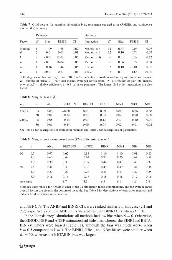
Table 7 GLM results for marginal simulation bias, root mean squared error (RMSE), and confidenceinterval (CI) accuracy

Deviance Deviance

Factor df Bias RMSE CI Interaction df Bias RMSE CI

Method 6 1.09 1.68 0.69 Method ×β 12 0.64 0.06 0.07β 2 0.01 0.01 0.01 Method × k 12 0.10 0.70 0.07

k 2 <0.01 12.02 0.06 Method × H 6 0.01 0.38 0.12

H 1 <0.01 16.04 0.05 Method × μ· 6 0.06 0.22 0.08

μ· 1 0.16 1.44 0.05 β × μ· 2 0.10 <0.01 0.01

D 1 <0.01 0.33 0.04 k × H 2 0.01 1.63 <0.01

Total degrees of freedom (d f ) was 504. Factor indicates estimation methods plus simulation factors:H—number of strata, μ·—pair-total means, averaged across strata, D—distribution of pair-total means,ρ = exp(β)—relative efficiency, k—NB variance parameter. The largest 2nd order interactions are alsolisted

Table 8 Marginal bias in β

ρ, β μ· ANBF BETABIN BINOD BINRI NBc1 NBct NBF

1.5,0.4 5 0.03 −0.08 0.01 0.09 0.08 0.06 0.0050 0.01 −0.14 0.01 0.02 0.02 0.00 0.00

2.0,0.7 5 0.05 −0.14 0.01 0.13 0.13 0.10 −0.01

50 0.01 −0.24 0.00 0.04 0.02 −0.01 −0.02


Table 9 Marginal root mean squared error (RMSE) for estimators of β

H k ANBF BETABIN BINOD BINRI NBc1 NBct NBF

10 0.5 0.97 0.62 0.84 1.10 1.10 0.91 0.851.0 0.63 0.48 0.61 0.73 0.70 0.64 0.58

3.0 0.39 0.33 0.39 0.44 0.41 0.40 0.37

50 0.5 0.41 0.30 0.36 0.49 0.49 0.44 0.36

1.0 0.27 0.24 0.26 0.31 0.31 0.29 0.25

3.0 0.16 0.16 0.17 0.18 0.18 0.17 0.16

Ave. rank 4.1 1.7 3.3 6.3 6.1 4.2 2.4

Methods were ranked for RMSE in each of the 72 simulation factor combinations, and the average ranksover all factors are given at the bottom of the table. See Table 1 for descriptions of estimation methods andTable 7 for descriptions of parameters

and NBF CI’s. The ANBF and BINRI CI’s were ranked similarly in this case (2.1 and2.2, respectively) but the ANBF CI’s were better than BINRI CI’s when H = 10.

In the “consistency” simulations all methods had low bias when β = 0. Otherwise,the BINOD, NBF, and ANBF estimators had little bias, whereas the BINRI and BETA-BIN estimators were biased (Table 11), although the bias was much worse whenk = 0.5 compared to k = 3. The BINRI, NBc1, and NBct biases were smaller whenμ· = 50, whereas the BETABIN bias was larger.

123


Table 10 Marginal error in confidence intervals (CI’s) for β = log(ρ)

H k ANBF BETABIN BINOD BINRI NBc1 NBct NBF

10 0.5 0.06 0.05 0.16 0.06 0.11 0.11 0.161.0 0.06 0.04 0.14 0.07 0.08 0.08 0.15

3.0 0.06 0.01 0.11 0.09 0.06 0.06 0.15

50 0.5 0.03 0.13 0.17 0.03 0.03 0.06 0.13

1.0 0.03 0.09 0.13 0.03 0.04 0.04 0.13

3.0 0.03 0.03 0.09 0.03 0.03 0.04 0.13

Ave. rank 2.6 2.5 5.9 2.9 3.3 4.1 6.5

The error was the absolute difference in the simulated CI exceedance minus the nominal α value. Methodswere ranked for CI error in each of the 72 simulation factor combinations, and the average ranks over allfactors are given at the bottom of the table. See Table 1 for descriptions of estimation methods and Table 7for descriptions of parameters

Table 11 Marginal bias in β when H = 50, 000

k μ· ρ, β ANBF BETABIN BINOD BINRI NBc1 NBct NBF

0.5 5 1.5,0.4 0.03 −0.15 0.01 0.13 0.12 0.11 −0.03

2.0,0.7 0.06 −0.25 -0.01 0.22 0.21 0.18 −0.05

50 1.5,0.4 0.01 −0.21 0.00 0.04 0.03 0.02 −0.01

2.0,0.7 0.02 −0.35 0.01 0.05 0.06 0.03 −0.02

3.0 5 1.5,0.4 0.01 −0.05 0.00 0.04 0.04 0.04 0.00

2.0,0.7 0.02 −0.08 0.01 0.07 0.07 0.07 0.00

50 1.5,0.4 0.00 −0.09 0.01 0.01 0.01 0.01 0.00

2.0,0.7 0.00 −0.17 0.00 0.02 0.01 0.01 −0.01


5.4.3 Robustness simulations

We focus on the ANBF, BETABIN, and BINRI methods which the results in Sect. 5.4.2suggest are most reliable overall. The method, size of β and O DT were the mostimportant factors in the ANOVA for bias and CI coverage. When the distributionalassumption underlying each method matched the O DT then the bias was lowestand CI coverage most accurate (Table 12). BINRI was the most bias robust method

Table 12 Bias in β and CI coverage error when β = 0.69; that is, ρ = 2

Bias CI coverage accuracy

O DT ANBF BETABIN BINRI ANBF BETABIN BINRI

B B 0.29 0.00 0.08 0.08 0.02 0.05B N −0.08 −0.26 −0.01 0.05 0.07 0.05NB 0.03 −0.19 0.08 0.05 0.05 0.05

O DT = B B indicates Beta-Binomial variation, O DT = B N indicates Binomial-normal variation, andO DT = N B indicates Negative Binomial variation

123


among the three. The BETABIN method produced the most accurate CI’s overall. Itsaverage rank was lowest, followed BINRI and ANBF; however, when H = 50 theBINRI method produced the most accurate CI’s with lower average rank. Similar toSect. 5.4.2, the BETABIN bias and CI accuracy was worse for larger values of H orμ· when O DT = NB or B N . This method performed more poorly when there wasmore data.

6 Discussion

We conclude overall based on the marginal simulations that the ANBF method pro-vided the best statistical inferences about the ratio of means from NB paired countdata. This method had lower bias and better CI accuracy, especially when H is fairlylarge. The NBF method resulted in inaccurate and too narrow CI’s because of bias inthis estimator of k. The commonly used BINOD method also produced too narrowCI’s. The BINRI method provided less reliable inferences when H = 10. Estimatesof the random effect variance were erratic with small sample sizes, and this affectedthe reliability of inferences about β. The BETABIN method advocated by Miller etal. (2010) produced good results overall in terms of RMSE, but the method seems tohave a bias that increases with NB sample size (i.e. H or μ·), and this bias seriouslyaffects the accuracy of associated CI’s. For comparative fishing studies this means thatthe BETABIN approach results in more biased estimates of β and ρ when the numberof tows or catch rates are larger, which is a situation where one typically hopes formore reliable estimation of ρ.

Our NB simulations results for the BINRI and BINOD methods were not consistentwith Cadigan and Dowden (2010). They showed using marginal simulations that theBINOD estimator of β had large negative bias when the over-dispersion was large.We did not find this result. Our NB marginal simulations indicated that the BINODestimator was unbiased. The difference is related to the type of Poisson over-dis-persion. Cadigan and Dowden (2010) simulations were based on Binomial-normalmixture model. In our robustness simulations the BINOD had a large negative biaswhen k = 0.5 similar to Cadigan and Dowden (2010). Hence, the source of Poisson-overdispersion is important to understand in order to recommend the most appropriateapproach. If there is uncertainty about the form of the Poisson over-dispersion thenthe BINRI is a good choice. The BINRI is a Binomial-normal mixture model, and itprovided unbiased estimates when the over-dispersion was generated using the samemechanism. It also resulted in lower biases, when the over-dispersion was mis-speci-fied, compared to the ANBF and BETABIN methods.

The conditional simulations demonstrated that conditional inferences based on NBpaired counts are sensitive to the differences in the paired totals and their means (i.e. thand μh·). This is different from the Poisson case in which the conditional distributionis Binomial and does not involve the μh· nuisance parameters. In this case it is com-mon to condition and th’s are treated like sample sizes that define the precision of theinferences. Severini (2000) referred to such statistics as ancillary for the parameter ofinterest (e.g. ρ) in the presence of the nuisance parameters. Statistical inferences arespecific to the observed values of t1, . . . , tH ; that is, frequency properties of estimators

123


are evaluated only with respect to the subset of Poisson paired count data whose pairedtotals are identical to those observed. This makes the inference more relevant to thedata at hand, and is a compromise between Bayesian and frequentist inference (e.g.Ghosh et al. 2010). If the estimator and CI’s are know to be unbiased for the observedvalues of t1, . . . , tH then the inferences can be considered very reliable for the data athand. If the estimator and CI’s are unbiased for many other values of t1, . . . , tH thenthe method is reliable.

The relevance arguement for conditioning is just as strong for NB paired counts.However, we cannot suggest a reliable conditional inference method, and the th’s can-not be treated like sample sizes. The accuracy of inferences for NB counts conditionalon the the th’s depends on the values of the μh· parameters. If differences between thand μh· are large and consistent among strata then inferences can be very unreliable.If these differences vary randomly between strata then inferences may be more reli-able. This occurred in our marginal simulations, although it can be argued that thesesimulations are less relevant because the values of th’s differed from those observed.Further research is required to find more relevant and reliable inference methods. Atleast our results have provided additional clarity about how statistical results shouldbe interpreted for NB paired counts.

When sample sizes are large then residual analyses can be used to diagnose thebasic form of Poisson overdispersion. However, unrealistically large sample sizes willbe required to diagnose the exact form. For example, it is unlikely that we would beable to distinguish between a Binomial-Normal mixture model and a Poisson-Gammamixture model (i.e. NB model). With small sample sizes then it may be difficult todiagnose even the basic form, such as whether the counts have NB1 or NB2 variability.Robustness is particularly important in this situation.

Estimates of β may also be improved if the dimension of the strata nuisance param-eters (μh·) could be reduced. It may be sensible to model μh· as a low-dimensionfunction of some covariates. Many fish surveys are stratified in contiguous areas ofsimilar depths, and it may be reasonable to assume that fish densities (i.e. λh in Eq. 1)are iid within these survey strata. This would reduce the dimension of {μ1·, . . . , μH ·}and provide more information to estimate these parameters, and k, in the NBc, NBFand ANBF methods.

Acknowledgments We thank two anonymous referees whose comments helped improve this manuscript,and to Dr. Chris Legault for reviewing an earlier version. This research work was funded by a grant fromthe Natural Sciences and Engineering Research Council of Canada.

7 Appendices

7.1 NBc probability mass function

To compute the NBc probability, let p(y) = Pr(Y1 = y|Y· = t) and

r(y) = p(y)/p(y − 1)

=(

pq

) (qμ·+kpμ·+k

) (y+k−1

y

) (t−y+1t−y+k

)(9)

123


A simple formula for p(y) is

p(y) = c(y)∑ty=0 c(y)

,

where c(y) =y∏

i=1r(i) for y > 0 and c(0) = 1.

7.2 NBc moments

When p = q then, using (9),

{(t + k)(y + 1)− (y + 1)2

}p(y + 1) = (k + y)(t − y)p(y). (10)

We use this relationship to derive the second moment of X ≡ Y1|Y· = t . After mul-tiplying both sides of (10) by y + 1 and summing from 0 to t − 1, we can showthat

(t + k)E(X2)− E(X3) = (tk + t + k)t/2 + (t − k − 1) E(X2)− E(X3).

This relationship can be simplified to give

E(X2) = t (tk + t + k)

2(2k + 1).

The variance is

V ar(X) = V ar(Y1|Y· = t) = t (2k + t)

4(2k + 1).

7.3 NB1 conditional moments

If Yh1 and Yh2 are NB1 rv’s with means μhi and variances (1 + φ)μhi then the con-ditional moments are very different than the NBc (i.e. NB2 conditional distribution)moments. The NB1 probability distribution function is given by (5) with k = μhi/φ.Note that in this case the k parameter is different for Yh1 and Yh2. Using methods sim-ilar to those outlined in Sects. 7.1 and 7.2, we can show that E(Yh1|Yh· = th) = th pand

V ar(Yh1|Yh· = t) ={

1 + (th − 1)

1 + μh·/φ

}th pq. (11)

In this case Poisson over-dispersion does not affect the conditional mean but doesinflate the conditional variance relative to the Binomial result when th > 1. Note that(11 ) is the same as the Beta-Binomial variance; however, the μh· term will differ

123


between pairs. If the Binomial over-dispersion term φ∗h = μh·/φ in (11) is assumed to

be constant across pairs, i.e. φ∗1 , . . . , φ

∗H = φ∗, then we have the standard Beta-Bino-

mial variance,

V ar(Yh1|Yh· = t) ={

1 + (th − 1)

1 + φ∗

}th pq.

However, this assumption implies that the unconditional variance is V ar(Yhi ) =(1 + μh·/φ∗)μhi and it does not make sense why the unconditional variance of Yh1should depend on μh2, and vice-versa.

7.4 Profile likelihood

We denote the likelihood of the parameters p, k and μ1·, . . . , μH · based on the fullset of H pairs of counts {(y11, y12), . . . , (yH1, yH2)} as l(p, k, {μh·}H

h=1). The profilelikelihood for p and k is l(p, k, {μh·(p, k)}H

h=1), where μh·(p, k) is the mle for fixedvalues of p and k. The kernel of the likelihood for μ1·, . . . , μH · treating p and k asfixed is

l({μh·}H

h=1

)=

∑h

{yh· log (μh·)− (k + yh1) log (k + pμh·)

−(k + yh2) log (k + qμh·)} .The score function for μh· is

S(μh·) = ∂l({μh·}H

h=1

)∂μh·

= p(yh1 − pμh·)vh1

+ q(yh2 − qμh·)vh2

= pεh1

vh1+ qεh2

vh2

where εhi = yhi − μhi and

μhi ={

pμh·, i = 1qμh·, i = 2

, vhi = μhi (1 + μhi/k) ={

pμh·(1 + pμh·/k), i = 1qμh·(1 + qμh·/k), i = 2

.

μh·(p, k) is the root of S(μh·) = 0, which is also the root of

k (yh· − μh·)+ {yh· − μh· + μh· (1 − 2pq)− (pyh1 + qyh2)}μh· = 0. (12)

If k → ∞ or p = q = 1/2 then μh·(p, k) = yh·The approximate standard error for p is SE( p)

.= j−1/211 ( p, k) where

j (p, k) = −[∂2l

(p, k, {μh·(p, k)}H

h=1

)/∂p2, ∂2l

(p, k, {μh·(p, k)}H

h=1

)/∂p∂k

∂2l(

p, k, {μh·(p, k)}Hh=1

)/∂p∂k, ∂2l

(p, k, {μh·(p, k)}H

h=1

)/∂k2

].

Standard errors for β = log{

p/(1 − p)}

can be obtained using the delta method.

123


7.5 Adjusted likelihood

The adjusted likelihood is

lM (p, k) = l(

p, k, {μh·}Hh=1

)+ M(p, k)

where M(p, k) is the adjustment proposed by Severini (2000, Section 9.5.4),

M(p, k) = log

⎧⎨⎩

| jμ,μ(p, k, μ)|1/2∣∣∣Iμ,μ(p, k, μ; p, k, μ)∣∣∣

⎫⎬⎭ , (13)

jμ,μ(p, k, μ) is the μ,μ block of the observed information matrix, and

Iμ,μ(p, k, μ; po, ko, μo) = Eo {S(μ)So(μ)} .The μ,μ block of the observed information matrix is diagonal with h, h element,

jh,h=−∂S(μh·)∂μh·

= p2

vh1+ q2

vh2+ μ−1

h·

(2pεh1

vh1+ 2qεh2

vh2− p2μh·εh1

v2h1

−q2μh·εh2

v2h2

).

The profile mle for μh· implies that

S(μh·) = pεh1

vh1+ q εh2

vh2= 0,

where εhi = yhi − μhi (ρ, k). Hence,

jh,h(p, k, μ) =(

p2

vh1+ q2

vh2

)−

(p2εh1

v2h1

+ q2εh2

v2h2

)

Eo {S(μ)So(μ)} is also a diagonal matrix with h, h element

S(μh·)So(μoh·) = Eo

{(pεh1

vh1+ qεh2

vh2

) (poεoh1

voh1+ qoεoh2

voh2

)}

= ppo

vh1Eo

(ε2

oh1

voh1

)+ qqo

vh2

(Eoε2

oh2

voh2

)

= ppo

vh1+ qqo

vh2.

These results can be used with (13) to give

M(p, k) = 1

2

∑h

log

[(p2

vh1+ q2

vh2

)−

(p2εh1

v2h1

+ q2εh2

v2h2

)]

−∑

h

log

(p p

vh1+ qq

vh2

)(14)

123


7.6 Marginal mle of μh·

For simplicity we drop the h subscript when deriving the marginal mle of μh·. Thepdf of Y· = Y1 + Y2 is Pr(Y· = t) = ∑t

x=0 Pr(Y1 = x)Pr(Y2 = t − x),

Pr(Y· = t |p, k, μ·) = k2k (qμ·)t

�2(k) (pμ· + k)k (qμ· + k)t+k

t∑x=0

φ(x, μ·)

where

φ(x, μ·) = �(x + k)�(t − x + k)

�(x + 1)�(t − x + 1)

(p

q

)x (qμ· + k

pμ· + k

)x

.

Note that

∂φ(x, μ·)∂μ·

= (q − p) kxφ(x, μ·)(qμ· + k) (pμ· + k)

.

The kernel of the marginal loglikelihood for μ· is

l(μ·; Y· = t) = t log(μ·)− k log(pμ· + k)

−(t + k) log(qμ· + k)+ log

(t∑

x=0

φ(x, μ·)).

The score function can be written

∂l(μ·)∂μ·

= k

[μ· {tp − 2μ· pq + (q − p) E(Y1|Y· = t)} + k (t − μ·)

μ· (qμ· + k) (pμ· + k)

],

and the marginal mle of μ· is the solution to

μ·{tp − 2μ· pq + (q − p) E(Y1|Y· = t)

} + k(t − μ·

) = 0 (15)

This solution must be obtained numerically. Similar to the full sample case, whenk → ∞ or p = q then μ· = th·

A closed form expression for the marginal mle of μ· would greatly simplify esti-mation of p and k from the NBc distribution. A good approximation can be obtainedusing a Taylor’s series expansion of E(Y1|Y· = t) about about μ· = t . Let ϒ(μ·) =E(Y1|Y· = t). The first order approximation is

ϒ(μ·).= ϒ(t)+ ϒ

′(t)(μ· − t),

where

ϒ′(t) = ∂ϒ(μ·)

∂μ·

∣∣∣∣μ·=t

=∑t

x=0 xφ′(x, μ·)∑t

x=0 φ(x, μ·)−

∑tx=0 xφ(x, μ·)

∑tx=0 φ

′(x, μ·){∑t

x=0 φ(x, μ·)}2

= (q − p) k

(qt + k) (pt + k)

{ϒ2(t)− ϒ2(t)

},

123


and ϒ2(μ·) = E(Y 21 |Y· = t). The approximate marginal mle of μ· is the solution to

the quadratic equation

{(q − p) ϒ

′(t)− 2pq

}μ2· +

[(q − p)

{ϒ(t)− ϒ

′(t)t

}+ tp − k

]μ·

+kt = 0. (16)

If k → ∞ or p = q then the positive root of (16) is μ· = t .

References

Allison PD, Waterman RP (2002) Fixed-effects negative binomial regression models. Sociol Methodol32:247–265

Barndorff-Nielsen OE, Cox DR (1994) Inference and asymptotics. Chapman and Hall, LondonBataineh OM (2008) Estimating relative efficiency from paired-count data with over-dispersion, with appli-

cation to fishery survey calibration studies. M.A.S. practicum report, Memorial University of New-foundland, St. John’s, Newfoundland and Labrador, Canada

Bellio R, Sartori N (2006) Practical use of modified maximum likelihoods for stratified data. BiometricalJ 48:876–886

Broström G, Holmberg H (2011) glmmML: generalized linear models with clustering. R package version0.82-1. http://CRAN.R-project.org/package=glmmML

Cadigan NG, Walsh SJ, Brodie W (2006) Relative efficiency of the Wilfred Templeman and Alfred Needlerresearch vessels using a Campelen 1800 shrimp trawl in NAFO subdivision 3Ps and divisions 3LN.DFO Canadian Science Advisory Secretariat Research Document 2006/085. http://www.dfo-mpo.gc.ca/csas/Csas/DocREC/2006/RES2006_085_e.pdf. Accessed January 2010

Cadigan NG, Dowden JJ (2010) Statistical inference about relative efficiency from paired-tow survey cali-bration data. Fish B 108:15–29

Cadigan NG (2011) Confidence intervals for trawlable abundance from stratified-random bottom trawlsurveys. Can J Fish Aquat Sci 68:781–794

Cameron AC, Trivedi PK (1998) Regression analysis of count data. Cambridge University Press, CambridgeCox DR (2006) Principles of statistical inference. Cambridge University Press, CambridgeCox DR, Snell EJ (1989) Analysis of binary data. 2 edn. Chapman and Hall, LondonDahm E, Wienbecka H, West CW, Valdemarsen JW, O’Neill FG (2002) On the influence of towing speed

and gear size on the selective properties of bottom trawls. Fish Res 55:103–119Dowden JJ (2008) Generalized linear mixed effects models with application to fishery data. M.A.S. practi-

cum report, Memorial University of Newfoundland. St. John’s, Newfoundland and Labrador, Canada,p 128

Ghosh M, Reid N, Fraser DAS (2010) Ancillary statistics: a review. Statistica Sinica 20:1309–1332Gunderson DR (1984) Surveys of fisheries resources. Wiley, New YorkHausman J, Hall BH, Griliches Z (1984) Econometric models for count data with an application to the

patents-R&D relationship. Econometrica 52:909–938Lee HS (1996) Analysis of overdispersed paired count data. Can J Stat 24:319–326Lewy P, Nielsen JR, Hovgård H (2004) Survey gear calibration independent of spatial fish distribution. Can

J Fish Aquat Sci 61:636–647Lowry MS (1999) Counts of california sea lion (zalophus californianus) pups from aerial color photographs

and from the ground: a comparison of two methods. Mar Mamm Sci 15:143–158Martinsen GD, Driebe EM, Whitham TG (1998) Indirect interactions mediated by changing plant chemis-

try: beaver browsing benefits beetles. Ecology 79:192–200McCullagh P, Nelder JA (1989) Generalized linear models. 2 edn. Chapman and Hall, LondonMcCulloch CE, Searle SR (2001) Generalized, linear, and mixed models. Wiley, New YorkMiddlemas SJ, Stewart DC, Mackay S, Armstrong JD (2009) Habitat use and dispersal of post-smolt sea

trout Salmo trutta in a Scottish sea loch system. J Fish Biol 74:639–651Millar RB (1992) Estimating the size-selectivity of fishing gear by conditioning on the total catch. J Am

Stat Assoc 87:962–968

123

http://CRAN.R-project.org/package=glmmML

http://www.dfo-mpo.gc.ca/csas/Csas/DocREC/2006/RES2006_085_e.pdf

http://www.dfo-mpo.gc.ca/csas/Csas/DocREC/2006/RES2006_085_e.pdf


Miller TJ, Das C, Politis PJ, Miller AS, Lucey SM, Legault CM, Brown RW, Rago PJ (eds) (2010) Esti-mation of Albatross IV to Henry B. Bigelow calibration factors. Northeast Fish Sci Cent Ref Doc.10-05, p 233. Available from: National Marine Fisheries Service, 166 Water Street, Woods Hole, MA02543-1026, or online at http://www.nefsc.noaa.gov/nefsc/publications/

Pelletier D (1998) Intercalibration of research survey vessels in fisheries: a review and an application. CanJ Fish Aquat Sci 55:2672–2690

R Development Core Team (2011) R: a Language and environment for statistical computing. R Foundationfor Statistical Computing, Vienna, Austria. ISBN 3-900051-07-0. http://www.R-project.org/

Reid N (1995) The roles of conditioning in inference. Stat Sci 10:138–199Sartori N (2003) Modified profile likelihoods in models with stratum nuisance parameters. Biometrika

90:533–549Severini TA (2000) Likelihood methods in statistics. Oxford University Press, OxfordSolís-Trápala IL, Farewell VT (2005) A note on robust inference from a conditional poisson model. Bio-

metrical J 48:117–130Schreibman T, Friedland G (2004) Use of total lymphocyte count for monitoring response to antiretroviral

therapy. Clin Infect Dis 38:257–262Teunis PFM, Evers EG, Slob W (1999) Analysis of variable fractions resulting from microbial counts.

Quant Microbiol 1:63–88

Author Biographies

N. G. Cadigan graduated in statistics from Memorial University, Canada, in 1990. In the same year hejoined Fisheries and Oceans Canada (DFO) at the Northwest Atlantic Fisheries Center in St. John’s,Newfoundland. In 1994 he left DFO to start a Ph.D. in statistics at the University of Waterloo (UW),Ontario, Canada. He returned to DFO in 1996 and received his Ph.D. from UW in 1999. Since then he hasbeen a research scientist with DFO. His research activities are focused on improving the quantitative basisfor fish stock assessment and sustainable fisheries.

O. M. Bataineh graduated in applied mathematics from Jordan University of Science & Technology,Jordan, in 1999. In 2008, he received a M.Sc. degree in statistics from Memorial University of Newfound-land, Canada, under the supervision of Dr. Noel Cadigan. Then he joined University of Saskatchewan,Canada, as a Ph.D. candidate in Statistics. He is expected to finish the Ph.D. degree in 2012.

123

http://www.nefsc.noaa.gov/nefsc/publications/

http://www.R-project.org/

inference about the ratio of means from negative binomial paired count data

Documents