Abstract— The Conductivity, Temperature, and Depth (CTD)

sensor is one of the most used instruments in the Oceanographic field. These devices are the number one, most important sensor for any research of the ocean depths. CTD measurements are found in every marine related institute and navy throughout the world because they are used to produce the salinity profile for the area of the ocean under investigation. In order to deploy large numbers of CTD sensors, an inexpensive version is needed, especially if used as a one-time (throw-away) system. Oceanographic institutes and navies require instruments such as these that are reliable, accurate, precise and inexpensive.

The CTD developed in this paper is low cost and disposable that can be easily and rapidly deployed to obtain measurements throughout the earth’s oceans. Five (5) specific specifications for the device (ECS Unit Sensor) were paramount: 1) Its weight had to be under 5-lb (2.27-kg) maximum, but ideally as close to 1 to 2-lb (0.45-kg to 0.9-kg) as possible; 2) Its dimensions must be no bigger than 10-in (25-cm) in height and 3-in (7.6-cm) in diameter; 3) It must be reasonably priced to be expendable; 4) It must have wireless communication; and 5) It only has to record the top 10-m of the water column.

This paper describes the design, development, construction and testing of the Expendable Conductivity Sensor Unit (ECS Unit), which when deployed, takes multiple snapshots of the water profile and sends its data out via a satellite communications chip. The ECS Unit was tested against other CTDs for accuracy. When compared to the other expendable CTDs the ECS Unit, along with being much more economical, is able to provide more snapshots than any other expendable CTD instrument currently available on the market. The CTD instrument (ECS Unit Sensor) developed in this project costs around $982.00 per unit to make.

Index Terms— conductivity, CTD, depth, expendable,

temperature,

This work was submitted on July 25, 2013 and was supported in part by

the United States Navy (Naval Surface Warfare Center Panama City Division (NAVSEA-PCD)).

S. L. Wood, is the Ocean Engineering program chair at Florida Institute of Technology, Department of Marine and Environmental Systems, Melbourne, FL 32901 USA (e-mail: swood@fit.edu).

R. Paradis, graduated with his Masters from Florida Institute of Technology and currently is an engineer at General Dynamics - Electric Boat, 75 Eastern Point Rd, Groton, CT 06340 USA (email rparadis@gdeb.com).

I. INTRODUCTION The CTD obtains the in situ salinity and temperature at a

specific depth to provide parameters for various uses such as determining the speed of sound at the depth. This information is a key part in understanding deep ocean currents and the ocean's acoustical properties. While research of the deep sea currents is important to oceanographers; the Navy is more interested in the acoustical properties of the ocean. These properties play an integral role for SOund Navigation And Ranging (SONAR) and are used to help determine the vibration signatures for underwater vehicles. The cost of the standard CTD instruments, whether expendable or not, is very expensive. In order to deploy large numbers of CTD sensors, an inexpensive version is needed, especially if used as a one-time (throw-away) system.

II. CTD'S Scientists use CTDs to get the salinity profile of a water

column in the ocean. These sensors give scientists a precise and comprehensive charting of the distribution and variation of water temperature, salinity, and density that helps understand how the oceans affect life [1]. These properties help oceanographers study the ocean and understand how the density variations affect the acoustical properties of the water.

Generally CTDs are large, expensive, and are tethered to a support vehicle (i.e., the CTD is lowered down into the water column). However, CTDs can be small, e.g., the units used in an Autonomous Underwater Vehicle (AUV) Remotely Operated Vehicle (ROV), or glider, but as their size decreases cost increases. Consequently, due to their price CTDs are not usually expendable.

The main sensors that make up a standard CTD package include a temperature sensor, conductivity meter, and pressure sensor. The temperature sensor provides measurements at the instrument’s location in the water column and those readings help determining the salinity. The conductivity meter measures conductance, which is the amount of electrical current that can pass through the water; and with a few calculations and input from the temperature probe, salinity is determined. The pressure sensor of course measures pressure, which is a function of depth. So, ultimately as the instrument is lowered into the water column it takes readings using the different sensors and through on-board calculations and data processing it provides temperature and salinity readings with

Inexpensive Expendable Conductivity Temperature and Depth (CTD) Sensor

R. Paradis, and S. L. Wood, Member, IEEE

respect to depth. These measurements giveproperties of sea water [1].

III. SALINITY Salinity provides the measurement of the a

mass, to a unit mass of seawater [2]. Thsalinity is important in understanding the effeinput and output to ocean dynamics and ph[3]. One of the most important physical pscientist is the ocean water’s density. This diacoustical properties of the ocean with whsound is calculated along with the sound refraction/diffraction properties. The speed oimportant property for the scientist, which iseqn. 1 provided by Hermin Medwin using”T”, depth ”z”, and salinity of the water ”S” [

c = 1449.2 +4.6T −0.055T 2 +0.00029T 3 +(1.34 (S −35)+0.16z

Salinity plays a key role in the health of va

around the ocean (e.g., coral reefs), slitemperature and salinity can wreak havoc oOceanographers are also interested in the salibecause along with water temperature, itdensity of the ocean water. The salinity snapshot of the density variations in the oceanand those profiles are important since as the oor salinity increases, the ocean water becomless dense. The change in water density dcirculation at greater depths more than wind dnear the surface [6]. These salinity profileimportant in understanding the ocean. By keeocean’s surface salinity/density, scientists fluctuations in the water cycle and get a bettof how the ocean interacts with various englobal scale [3].

To measure salinity, the following equatiBibby Scientific [7] are used. A probe with a“K” will have to be known. “K” is calculatedistance between the probes (D) by the surprobes (A):

K = D /A

By passing a known current and voltage awhile submerged in the salt water a conducmeasured in units of Seimens (S’). To get the electrical current I is divided by the known

G = I/V

With the conductance known and the proknown, conductivity (C) can be calculated conductance by the probe cell constant “K”:

C = G(K)

Once conductivity is calculated it is converte(R), which is the reciprocal of conductivity.

e insight into the

amount of salt by he ocean surface ects of fresh water hysical properties properties for the irectly affects the

hich the speed of wave reflection/

of sound “c” is an s calculated using g the temperature [4].

4−0.010T ) (1)

arious ecosystems ight changes in n coral reefs [5]. nity of the ocean, t determines the

profiles give a n at that location, ocean water cools

mes either more or drives the ocean driven circulation es are extremely eping track of the can monitor the ter understanding

nvironments on a

ions provided by a set cell constant d by dividing the rface area of the

(2)

across the probe ctance reading is conductance (G), n voltage (V) :

(3)

obe cell constant by dividing the

(4)

ed into Resistivity

R = 1/C

With resistivity and temperatcalculated using the Practical Salinequation by Edward Lewis [2] (Eother additional variables: a temperof the CTD instrument. The unity isconductivity value of a known soluticonductivity reading of the solutivariable used in the equation ofcombination of those variables and PSS equation is calculated.

where:

a0 = 0.0080, a1 = -0.1692, a2 = 25a4 = -7.0261, a5 = 2.7081 k is the sensors measure of unity RT is the resistivity of the water the temperature of the water sampb0 = 0.0005, b1 = -0.0056, b2 = -0b4 = 0.0636, b5 = -0.0144 Equation 6 is valid for temperatu

�C and salinity between 2 and 42 [is good for a wide salinity range,conductivity of the sea water mustconstant if the instrument cannotcurrent it can pass across the prosaltwater should be 10, for brackiwater 0.1 cell constant [7]. Since thfor saltwater, the cell constant thatconstant.

IV. CTD TCTDs come in all shapes and siz

CTD (the most basic and popular tyFloats, and the expendable eXpendcasting methods include ship assistand remote sensing. Ship assisted complete a CTD cast (i.e., the lowCTD through the water column). operation of the CTD is by AUV, RO

Most ship assisted CTDs are larrecorded via communications cablechip. These systems require a cable in order to download the measuremcommunications cable is used, scienproperties in real time. A standardwater depth, usually requires a coucomplete set of data. Small, low-pused on expendable CTDs or autonprofiling floats, AUV’s, Expendable

(5)

ture the salinity (S) is nity Scale of 1978 (PSS)

Eqn. 6). This equation has rature reading and unity k s determined by taking the ion and comparing it to the on. This ratio is the last f the PSS [7]. With the a few given constants, the

(6)

5.3851, a3 = 14.0941

sample at temperature T is ple .0066, b3 = -0.0375

ures between -2 �C and 35 [2]. Although this equation the probe measuring the t have the appropriate cell t regulate the amount of obes. The cell constant of sh water 1, and for fresh

he ECS Unit was designed t was used was the k =10

TYPES zes, ranging from a casting ype), the autonomous Argo dable CTD (XCTD)s. CTD ted casting/manual casting casts use manual input to wering and raising of the

For remote sensing, the OV, or glider. rge and measurements are e or logged on a memory to be plugged into the unit

ments for analysis. When a ntists can observe the water d CTD cast, depending on uple of hours to collect a powered CTD sensors are nomous platforms such as e or moored profilers [1].

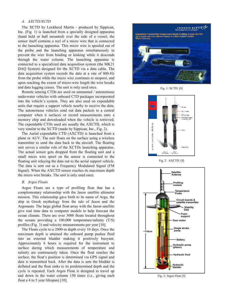
A. AXCTD/XCTD The XCTD by Lockheed Martin - produced by Sippican,

Inc. (Fig. 1) is launched from a specially designed apparatus (hand held or hull mounted) over the side of a vessel; the sensor itself contains a reel of a micro wire that is connected to the launching apparatus. This micro wire is spooled out of the probe and the launching apparatus simultaneously to prevent the wire from binding or kinking while it descends through the water column. The launching apparatus is connected to a specialized data acquisition system (the MK21 DAQ System) designed for the XCTD via a data cable. The data acquisition system records the data at a rate of 800-Hz from the probe while the micro wire continues to unspool, and upon reaching the extent of micro-wire length the wire breaks and data logging ceases. The unit is only used once.

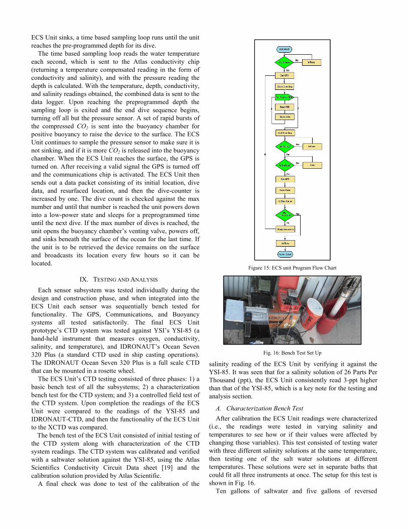
Remote sensing CTDs are used on unmanned / autonomous underwater vehicles with onboard CTD packages incorporated into the vehicle’s system. They are also used on expendable units that require a support vehicle nearby to receive the data. The autonomous vehicles send out data packets to a central computer when it surfaces or record measurements onto a memory chip and downloaded when the vehicle is retrieved. The expendable CTDs used are usually the AXCTD, which is very similar to the XCTD (made by Sippican, Inc., Fig. 2).

The Aerial expendable CTD (AXCTD) is launched from a plane or AUV. The unit floats on the surface using a wireless transmitter to send the data back to the aircraft. The floating unit serves a similar role of the XCTDs launching apparatus. The actual sensor gets dropped from the floating unit and a small micro wire spool on the sensor is connected to the floating unit relaying the data out to the aerial support vehicle. The data is sent out as a Frequency Modulated Signal (FM Signal). When the AXCTD sensor reaches its maximum depth the micro wire breaks. The unit is only used once.

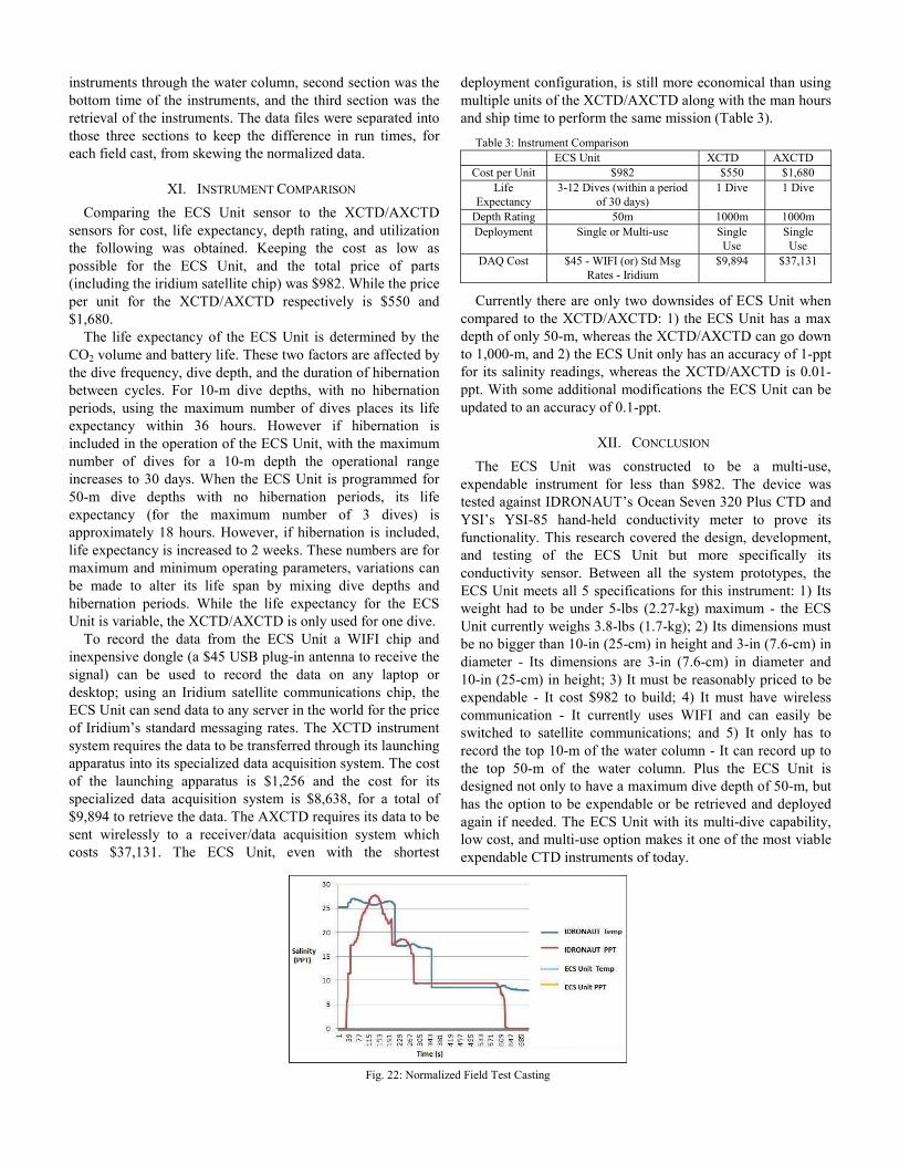
B. Argos Floats Argos Floats are a type of profiling float that has a

complementary relationship with the Jason satellite altimeter mission. This relationship gave birth to its name of Argo, the ship in Greek mythology from the tale of Jason and the Argonauts. The large global float array with the Jason satellite give real time data to computer models to help forecast the ocean climate. There are over 3000 floats located throughout the oceans providing a 100,000 temperature/salinity (T/S) profiles (Fig. 3) and velocity measurements per year [10].

The Floats cycle to a 2000-m depth every 10 days. Once the maximum depth is attained the onboard pump pushes fluid into an external bladder making it positively buoyant. Approximately 6 hours is required for the instrument to surface during which measurements of temperature and salinity are continuously taken. Once the float reaches the surface, the float’s position is determined via GPS signal and data is transmitted back. After the data is sent the bladder is deflated and the float sinks to its predetermined depth and the cycle is repeated. Each Argos Float is designed to travel up and down in the water column 150 times (i.e., giving each float a 4 to 5 year lifespan) [10].

Fig. 1: XCTD: [8]

Fig. 2: AXCTD: [8]

Fig. 3: Argos Float [9]

C. AUV or Glider CTDS AUV’s and gliders are used in every ocean around the

world. AUV’s, such as the Remote Environmental Monitoring Units (REMUS), actively roam the oceans days or weeks at a time working on missions that scientists have programmed. Autonomous underwater gliders are similar to the standard AUV, but generally are much smaller and use considerably less power. Rather than using thrusters, they dynamically adjust their buoyancy and convert the upwards or downwards motion, from the change in buoyancy, to forward motion with the pitch of their wings as an airplane does. The only difference is that the plane usually stays level while the underwater glider’s center of gravity changes thus changing the glider’s angle, e.g., the Slocum glider (Fig. 4).

AUV’s typically have a higher payload capacity and therefore can carry higher grade CTDs than gliders. For example, the SBE 49 Fast-CAT CTD from Sea-Bird Electronics, generally used in AUVs like the Bluefin Robotics AUV’s, has a data logging rate of 16-Hz. This CTD, depending on the model, has depth ratings up to 7000-m; and a resolution of 0.00005 Seimens per Meter (S’/m).

This CTD is directly powered from the AUV’s battery bank. Gliders like the Slocum Glider, mindful of their payload weight, cannot carry such high end CTDs. Generally gliders tend to use CTDs like the Glider Payload CTD from SEA-Bird Electronics, which has a 1-Hz data logging rate and a depth rating to 1500-m; and a resolution of 0.0003-(S’/m). The lack of power available to the CTD on gliders requires the CTD to have its own battery pack to power it for up to 45 days. [12]

D. Moored Profilers A Moored Profiler is a CTD that travels up and down the

water column attached to a subsurface mooring, using a traction motor to travel up and down the mooring line. The sub-surface mooring stretches to the seafloor (Fig. 5) and is used in all regions of the ocean (i.e., from shallow coastal waters to deep open ocean waters). This type of CTD profiler stores its data on-board for the duration of its deployment and is offloaded when the instrument is recovered. [14]

V. BUOYANCY CONTROL Buoyancy control is the ability to maintain negative,

neutral, or positive buoyancy while in the water column. Buoyancy control is the adjustment of the water displacement/ density of the platform on which the CTD unit is mounted. For AUVs, buoyancy control comes from a neutral buoyancy design and through the use of thrusters to determine water column position. Gliders control their buoyancy by either adjusting an inflatable bladder or by manipulating materials that can adjust their density such as thermal waxes and then use the pitch of their wings to control its ascent/descent in the water column [11]. The Argos Float changes its density by pumping fluid out of its body into an external air bladder. As long as the water displaced/density can be manipulated, buoyancy control has been achieved.

VI. DEVELOPMENT

A. Design Considerations The five (5) requirements for the ECS-Unit are: 1) Its

weight must be under 5-lb (2.27-kg) maximum, but ideally as close to 1 to 2-lbs (0.45-kg to 0.9-kg) as possible; 2) Its dimensions must be no bigger than 10-in (25-cm) in height and 3-in (7.6-cm) in diameter; 3) It must be reasonably priced to be expendable; 4) It must have wireless communication; and 5) It must record the top 10-m of the water column. Secondary requirements are: 6) it should have a 50-m depth rating; and 7) it could be reused if retrieved.

The physical design of the ECS Unit’s housing was determined by the shape of an AUV’s payload bay that would hold the ECS Unit (i.e., a bay of 3-in (7.6-cm) diameter by 10-in (25-cm) long) gave the ECS Unit its size and shape (Fig. 6). Due to the size restraint, the ECS Unit telescopes to allow the bottom of the unit to slide up into the buoyancy chamber. When deployed, the ECS Unit expands when the buoyancy chamber is inflated.

The operation of the ECS Unit is designed to be deployed via an aerial vehicle or AUV. To prevent early activation the unit is powered on only when a pair of water-contacts becomes submerged for any period longer than a few seconds. When the unit is deployed and becomes activated, it begins its

Fig. 4: Slocum: [11]

Fig. 5: Sub Surface Moored Profiler: [13]

mission as depicted in Fig. 7. After the ECS it releases enough compressed air to create poWhen the unit reaches the ocean surface it elocation and makes contact with a T(TACSAT) (one of 4 in a series of U.S. militreconnaissance and communication satellites)

The device starts its first dive by openinchamber’s venting solenoid valve allowing thflood, creating negative buoyancy. While thea specified depth, readings are obtained and uspecified depth releases compressed CO2 gasWater is expelled creating positive buoyandevice to ascend to the surface where the nexobtained and data is transmitted to the transmission the unit goes into a preprogramuntil it is time for the next dive. Upon westablishes another GPS location and repeats ECS Unit developed in this research is abledive cycles to a 10-m depth or 3 dive cycles50-m depth rating.

B. Buoyancy System As stated before, the buoyancy system f

uses compressed CO2 gas to displace waterchamber and opens a solenoid valve to vent thbuoyancy chamber to flood the chamber wThis complete system uses one 16-g CO2 cpuncture device, one pressure regulator, twoand a flood-able chamber. The 16-g CO2 cawhen full is nominally around 900 to 100kg/cm). The 16-g CO2 canister’s pressure posthe 5-V miniature solenoid valves with their 1rating, which was remedied by a pressure reregulators are used to reduce the presdownstream components of a pneumatic circu

The pressure regulator was made out of 1-ibrass stock with a male thread to attach tshortening the device. From the input side o0.040-in (1-mm) hole was made to connect twith an interior diameter of 0.625-in (accommodated a 0.5-in (13-mm) seat. Ussupply an additional 8-lbs (3.6-kg) of freduction of 80-psi (5.6-kg/cm) was achieregulator worked, it will be replaced by a lshelf version for higher quality when the ECproduction. The designed pressure regulator stage regulator reducing the 1000-psi to 80kg/cm) (size limitations prevented a reduction). This single stage pressure regulaabout a 100-psi (7-kg/cm) remaining in the two stage pressure regulator is recommendedthe compressed air in the ECS Unit.

The buoyancy system allows the ECS Ucomplete 12 dive cycles for a 10-m depth, or 50-m. The following equations and data conexpand on how these numbers were achieved.

First, take the 16-g of compressed CO2 an

Unit is deployed ositive buoyancy. establishes a GPS Tactical Satellite tary experimental ). ng the buoyancy he air chamber to e unit descends to upon reaching the s into a chamber. ncy allowing the xt GPS position is TACSAT. After

mmed sleep period waking, the unit all the steps. The

e to complete 12 s to its maximum

for the ECS Unit r in its buoyancy he CO2 gas in the

with water again. canister, one CO2 o solenoid valves, anister’s pressure

00-psi (63 to 70-sed a problem for 100-psi (7-kg/cm) egulator. Pressure ssure acting on uit [11]. in (2.5-cm) round the CO2 canister, of the regulator a the reduction side (16-mm), which sing a spring to force a pressure eved. While this low cost, off-the-CS Unit goes into

is a basic single 0-psi (70 to 5.6-further pressure

ator design leaves CO2 canister. A

d to optimally use

Unit to be able to r 3 dive cycles for nstants from [15] . nd convert it to a

molecular weight: 16gx(1-mole/44-gNext, take that weight and calcu

exhaust ambient pressure and divvolume needed in the buoyancy chabuoyant and subtract 1 cycle for a fadive depth exhaust ambient pressureV = [(0.3636mole)(0.0822)(293)]/2

= 13 − 1 = 12 Dive C

For a 50-m dive depth exhaust aatm: V = [(0.3636mole)(0.0822)(293

= 4 − 1 = 3 Dive Cap

VII. CTD SE

An inexpensive CTD sensor is rebe a success. Multiple designs weconcept CTD design was obtained.

Fig. 6: ECS unit compressed an

Fig. 7: ECS Sequenc

g) = 0.3636-mole. ulate the volume (L) at the vide it by the amount of amber to make it positively actor of safety: For a 10-m e will be 2-atm: 2atm = 4.38L.

Capability (7)

mbient pressure will be 6-3)]/6atm = 1.46L .

pability (8)

ENSOR quired for the ECS Unit to re tried before a proof-of-First, a linear 4-pin probe

nd expanded for storage

ce of Events

design was tried where the probes were placed in a line and spaced equally apart. This type of probe is optimum to get a stable conductivity reading from the water while avoiding electroplating the probes. In the four-pin probe design, the outermost probes alternate in pushing and pulling current through the water while the two middle probes read the voltage. The two probes reading the voltage at separate locations, gives a change in voltage over the distance between the probes. Combining the change in voltage with the known current being sent across the outermost probes produces the resistivity of the water and along with a temperature reading, salinity can be calculated by using the PSS equation. This design was abandoned since the readings were not stable. Next, a linear four-pin probe design with a four concentric circular pin design was tried (Fig. 8).

This four pin circular pin design proved to be more stable but the readings still fluctuated and required more calculations than what is normally used to get the resistivity of the water. Since there were multiple probe pins, the current flowing around each pin converted each pin to act like a magnet, which also changed the cell constant. The cell constant would have to be normalized for the current flow of an electrical dipole field [16]. This version was also abandoned and the next version was based on the usual two pin design.

The two pin design once again improved the readings but the still proved insufficient. The two pin CTD design was replaced by completely new CTD design that incorporated an Atlas conductivity chip. The Atlas is a small embedded CTD chip that any probe could be hooked up to it as long as it had the same cell constant it was designed for (i.e., a cell constant of 10 for solutions that have a high concentration of salt like oceanic waters). This new probe was designed to have the cell constant K = 10.

This new design for the CTD probe still proved difficult since the cell constant K = 10 was not easy to set up by hand. It needed to be very precise and accurate. First designed with two cylindrically shaped stainless steel pins set at a distance of one centimeter apart, the stainless steel quickly corroded as soon at a current was passed between them. These pins were upgraded to gold plated nickel pins that are slightly larger, and placed about two and a half centimeters apart. The gold plated nickel pins of this CTD probe also corroded, albeit at a much slower rate. The probe pins were then upgraded to platinum. As seen in Fig. 9, the pins were changed to the miniature flat bar shape in the existing probe. Each pin is 2-mm wide and 6.35-mm high, with a spacing of 12.7-mm in between. This was determined by using the cell constant value of K = 10 and working the equation backwards, using the known surface area of the pins, to get the distance between them.

VIII. SYSTEM ELECTRONICS INTEGRATION The ECS Unit consists of five primary electronic systems:

GPS, CTD, Communications, Data Logger, and Controller. Each serves a crucial role in the operation of the unit. The GPS system shows how the unit is drifting with the currents of the ocean and the location where each dive was performed.

The CTD system evaluates the water samples, and is the key system component of device. The communications system allows the data to be offloaded; but as a backup, a micro SD card is onboard to store all data in case of communication failure. Lastly, the controller of the device is a PIC18LF4520 microchip.

A. Global Positioning System The GPS was first established in 1978 by the United States

Department of Defense. By sending a signal to a minimum of four satellites, a position can be triangulated on the Earth’s surface down to about a 10-m radius [17]. GPS operations depend on a very accurate time reference, given by atomic clocks from the U.S. Naval Observatory, and each GPS satellite has atomic clock on board [18]. The ECS Unit uses the Venus GPS board from Sparkfun Electronics.

This GPS outputs the standard National Marine Electronics Association (NMEA) sentences with update rates up to 20-Hz. The GPS requires a regulated 3.3-V supply to operate, and when powered up uses up to 90-mA. The main NMEA identifying string of information sent by the Venus GPS is the GPRMC string. This string of information provides a valid signal indicator, date, time, latitude, longitude, speed, bearing, and magnetic variation. The valid signal indicator, date, time, latitude, and longitude used by the ECS Unit are obtained from this string using a GPS parse loop. The parse loop looks for the start of the GPRMC string and saves each character until it sees the end of the string. With the GPRMC string in memory, the parsing loop looks for commas that are used to separate the values of each data point. Using the commas the parse loop separates the data points that is wanted and discards those that are not.

B. Conductivity Temperature Depth Sensor The CTD is the system that handles the water sampling that

the unit was made for and uses the E.C. Circuit from Atlas

Fig. 8: 4 Pin Concentric Circular Probe

Fig. 9: New Probe for K=10

Scientific (Fig. 10). Atlas Scientific claims that the chip is accurate enough for lab work yet rugged enough for a long-term field deployment. Almost a plug-and-play device, it requires minimal calibration. With included calibration solutions, the sensor reads out the conductivity, total derived solids (referenced to KCL), and the salinity.

The Atlas chip outputs these values in a string that is parsed via a carriage return character at the end of the string. Unlike most chips outputting strings that end with the standard null character, the Atlas chip ends its strings with a carriage return. So a parse loop is used to save the string and look for when the data ends. The salinity values are derived from the Practical Salinity Scale. The ECS Unit uses one of the Atlas chip’s commands to take a temperature calibrated reading. After sending the ambient temperature value to the Atlas chip it responds by sending back the temperature calibrated reading. This process takes just under a second to accomplish and regulates the rate of sampling for the ECS Unit to 1-Hz as it descends through the water column.

C. Communications The communication system of the ECS Unit allows data to

be offloaded. The XBee chip from Digi (Fig. 11) uses a form of Wireless Fidelity (WIFI) called ZigBee Protocol and has a data transfer range of one hundred and twenty meters line-of-sight. To retrieve data via the XBee, the receiver must be located fairly close as the data transfer range is optimistic. Like the Venus GPS it is powered with 3.3-V and uses 200-mA when transmitting data.

The XBee chip when the ECS Unit is deployed will be replaced by an Iridium Satellite Communications Chip (Fig. 12). This chip is able to communicate with the NAVYs TACSAT network providing data access from the ECS Unit anywhere in the world.

D. Data Logging The data logging system is run by an open source data

logger “OpenLog” (Fig. 13). This logger takes any serial stream sent to it and logs it.

OpenLog logs continuously, but commands can be sent to it to initiate other operations, for example: sending the command ”new File” will create a new file named File and then sending the command, ”write” puts it back into logging mode again, in doing so, saves data to the new file. Cycling the power creates a new file named with incrementing numbers. The ease of use from OpenLog made it an easy choice to use for data logging operations.

E. Controller The controller for the system is a PIC18LF4520 chip from

Microchip (Fig. 14) (i.e., an 8-bit microcontroller that uses a 16-bit architecture [23]). The PIC18 family is one of the most popular chip families for embedded systems that support both 3-V and 5-V applications like the ECS Unit. The LF version of the chip has a power supply ranging from 2-V to 5.5-V and draws minimum current when compared to other chip families. This chip controls when the GPS, WIFI, CTD, and data logger are switched on and off, parses the GPS and Atlas

Chip output strings, writes/reads data to and from the data logger, and sends data out through the WIFI chip. This chip also is able to puts itself into sleep mode between dives and wakes up when it is time to start a new dive.

Two PIC18LF4520 chip problems arose during testing: 1) a memory problem (i.e., too much data to store on the onboard flash memory of each dive before transferring it to external memory); and 2) it had only one hardware data transfer port (i.e., the GPS, WIFI, CTD, and Data Logging systems all use this port and sometimes at the same time). The first issue was solved by saving the data to the data logger as it was sampled and the second issue was solved by setting up a secondary software data transfer port.

F. Software and Application When the ECS Unit is activated, a start-up sequence runs

followed by the main operation’s loop. The program exits only when the maximum number of pre-programmed dives is reached. This sequence of events is depicted visually in the flow diagram in Fig. 15. Upon activation the ECS Unit determines whether it is floating at the surface of the water by sampling the pressure sensor and if so obtains a GPS position. If the device is below the surface it inflates the buoyancy chamber and rises to the surface to make the satellite link where it makes contact with the satellite and obtains a GPS position, parses the GPS signal and records the date, time, and location. Once the information is recorded, the ECS Unit starts the dive sequence. The dive sequence consists of shutting down the communications chip and GPS chip, starting the continual background sampling of the pressure sensor, as well as venting the buoyancy chamber to start the dive. While the

Fig. 10: Atlas E.C. [19] Fig. 11: XBee WIFI: [20]

Fig. 12: Iridium [21] Fig. 13: OpenLog [22]

Figure 14: Pic chip [23]

ECS Unit sinks, a time based sampling loop runs until the unit reaches the pre-programmed depth for its dive.

The time based sampling loop reads the water temperature each second, which is sent to the Atlas conductivity chip (returning a temperature compensated reading in the form of conductivity and salinity), and with the pressure reading the depth is calculated. With the temperature, depth, conductivity, and salinity readings obtained, the combined data is sent to the data logger. Upon reaching the preprogrammed depth the sampling loop is exited and the end dive sequence begins, turning off all but the pressure sensor. A set of rapid bursts of the compressed CO2 is sent into the buoyancy chamber for positive buoyancy to raise the device to the surface. The ECS Unit continues to sample the pressure sensor to make sure it is not sinking, and if it is more CO2 is released into the buoyancy chamber. When the ECS Unit reaches the surface, the GPS is turned on. After receiving a valid signal the GPS is turned off and the communications chip is activated. The ECS Unit then sends out a data packet consisting of its initial location, dive data, and resurfaced location, and then the dive-counter is increased by one. The dive count is checked against the max number and until that number is reached the unit powers down into a low-power state and sleeps for a preprogrammed time until the next dive. If the max number of dives is reached, the unit opens the buoyancy chamber’s venting valve, powers off, and sinks beneath the surface of the ocean for the last time. If the unit is to be retrieved the device remains on the surface and broadcasts its location every few hours so it can be located.

IX. TESTING AND ANALYSIS Each sensor subsystem was tested individually during the

design and construction phase, and when integrated into the ECS Unit each sensor was sequentially bench tested for functionality. The GPS, Communications, and Buoyancy systems all tested satisfactorily. The final ECS Unit prototype’s CTD system was tested against YSI’s YSI-85 (a hand-held instrument that measures oxygen, conductivity, salinity, and temperature), and IDRONAUT’s Ocean Seven 320 Plus (a standard CTD used in ship casting operations). The IDRONAUT Ocean Seven 320 Plus is a full scale CTD that can be mounted in a rosette wheel.

The ECS Unit’s CTD testing consisted of three phases: 1) a basic bench test of all the subsystems; 2) a characterization bench test for the CTD system; and 3) a controlled field test of the CTD system. Upon completion the readings of the ECS Unit were compared to the readings of the YSI-85 and IDRONAUT-CTD, and then the functionality of the ECS Unit to the XCTD was compared.

The bench test of the ECS Unit consisted of initial testing of the CTD system along with characterization of the CTD system readings. The CTD system was calibrated and verified with a saltwater solution against the YSI-85, using the Atlas Scientifics Conductivity Circuit Data sheet [19] and the calibration solution provided by Atlas Scientific.

A final check was done to test of the calibration of the

salinity reading of the ECS Unit by verifying it against the YSI-85. It was seen that for a salinity solution of 26 Parts Per Thousand (ppt), the ECS Unit consistently read 3-ppt higher than that of the YSI-85, which is a key note for the testing and analysis section.

A. Characterization Bench Test After calibration the ECS Unit readings were characterized

(i.e., the readings were tested in varying salinity and temperatures to see how or if their values were affected by changing those variables). This test consisted of testing water with three different salinity solutions at the same temperature, then testing one of the salt water solutions at different temperatures. These solutions were set in separate baths that could fit all three instruments at once. The setup for this test is shown in Fig. 16.

Ten gallons of saltwater and five gallons of reversed

Figure 15: ECS unit Program Flow Chart

Fig. 16: Bench Test Set Up

osmosis filtered water were obtained from the local aquarium store and tested by a salinometer to have a salinity of 26-ppt. This was then divided into three separate solutions one of which the salinity was changed by diluting the solution with the reversed osmosis water to a salinity of 18-ppt. Then the reversed osmosis filtered water and the three saltwater solutions were stored in an air conditioned room to bring their temperature down to simulate normal ocean temperatures.

The first test to characterize the device was to measure the salinity of different saltwater solutions at the same temperature (22 oC). Freshwater was the first solution measured by all three instruments at the same time. After waiting a few minutes to allow the readings to stabilize, their readings were recorded. Each had an average reading of 0-ppt as would be expected for fresh water. This procedure was repeated for the 18-ppt and the 26-ppt solutions (Table 1).

Table 1: Characterization Test 1 Steady Temperature (20oC) − Variable Salinity

Solution IDRONAUT CTD YSI-85 ECS Unit RO (0-ppt) 0.042 0.1 3 18-ppt 18.128 18.5 21 26-ppt 26.174 26.7 29

For the reverse osmosis water the instrument readings were IDRONAUT-CTD: 0.042-ppt, YSI-85: 0.1-ppt, and the ECS Unit: 3.0-ppt; For the 18-ppt saltwater solution the IDRONAUT-CTD: 18.128-ppt, YSI-85: 18.5-ppt, and the ECS Unit: 21-ppt; For the 26-ppt saltwater solution the IDRONAUT-CTD: 26.174-ppt, YSI-85: 26.7-ppt, and the ECS Unit: 29-ppt. (Note: the ECS Unit consistently read 3-ppt higher than the other CTDs and is used to calculate the unity of the CTD sensor.)

The second part of the characterization test was to measure the salinity of the saltwater solution (26-ppt) at different temperatures. Simultaneously, all three instruments measured the solution at 19.5 oC. After waiting for a few minutes to allow readings to stabilize, the following were obtained: the YSI-85 and the IDRONAUT-CTD had an average reading of 26-ppt and the ECS Unit read 29-ppt. This procedure was repeated for 22.1 oC, 28.2 oC and again for or the 26-ppt solution. The salinity readings changed minimally, only the temperature changed (Table 2).

Table 2: Characterization Test 2A Steady Salinity (26-ppt) − Variable Temperature

Solution IDRONAUT-CTD YSI-85 ECS Unit 19.5 oC 26.173 26.6 29 22.1 oC 26.175 26.8 29 28.2 oC 26.176 26.7 29

The remaining 26-ppt saltwater solution that was kept in an air conditioned room was used to show the dynamics of the water while raising the temperature from 19 oC to 28 oC (e.g., to see how the readings would change when passing through a thermocline). In this test the ECS Unit was compared to the IDRONAUT-CTD only, since the YSI-85 could not record data automatically. The salinity readings changed minimally, only the temperature changed significantly (Fig. 17).

B. Controlled Field Test After successfully passing the characterization testing, the

ECS Unit underwent a controlled field test in the brackish water of the Indian River Lagoon, at the mouth of Crane Creek in Melbourne Florida.

The ECS Unit was tested against the IDRONAUT-CTD where three separate casts were performed off the dock. Each cast was compared individually and as an average between the two instruments. The two CTDs were lowered at the same time and rate to the bottom of the marina where they remained for enough time to obtain accurate readings (i.e., few seconds). These casts were performed to verify how the ECS Unit operates (Fig. 18-20 field casts). After each cast the logged data was saved to separate files for each instrument and the process repeated until all three casts were completed and their information gathered and logged.

X. ANALYSIS OF TEST DATA The test data gathered from all four tests performed on the

ECS Unit was compared to the data collected from the IDRONAUT as well as the YSI-85. It should be noted that the initial calibration of the commercial CTDs might have drifted over time and induced an error in the readings, but the focus of these tests was to look at the trend of the data. Any percent error in readings is easily fixable, but an error in the data trend is a fundamental issue.

During the initial bench test it was noted that the ECS Unit had a consistent reading of 3-ppt higher than the YSI-85, this was true of all the tests. The initial bench test and the first characterization tests were not graphed due to the data being recorded by hand and therefore not being continuously logged. This was also the case with the first half of the second characterization tests as well. However, the second half of the last characterization testing was recorded continuously; therefore this is where the graphical comparison begins for the ECS Unit. The data comparison was made between the instruments by observing and comparing their outputs through the graphical representation of their data.

Looking at the graph in Fig 21, the trend between the ECS Unit and the IDRONAUT-CTD is extremely similar (when not normalized the consistent offset can be seen and easily corrected). When the trends in Fig. 21 are overlaid onto each other, there is no discernible difference between the two outputs. The field test data shows that, between the IDRONAUT-CTD and the ECS Unit, the output readings still have a similar trend with the 3-ppt offset. The three separate casts performed during the controlled field test were averaged (to normalize the readings) and graphed. As with the characterization test, the normalized data from the field test showed that the trend between the two instruments was practically identical, with the only difference being the 3-ppt offset (Fig. 22).

When looking at the graph of the normalized field test data, the temperature and conductivity appear to have a stair like trend, this is due to the field test data being split into three sections. The first section covered the lowering of the

instruments through the water column, second section was the

Fig. 17: Characterization Test 2B

Fig. 18: Field Test Cast 1

Fig. 19: Field Test Cast 2

Fig. 20: Field Test Cast 3

Fig. 21: Normalized Characterization Test 2B

instruments through the water column, second section was the bottom time of the instruments, and the third section was the retrieval of the instruments. The data files were separated into those three sections to keep the difference in run times, for each field cast, from skewing the normalized data.

XI. INSTRUMENT COMPARISON Comparing the ECS Unit sensor to the XCTD/AXCTD

sensors for cost, life expectancy, depth rating, and utilization the following was obtained. Keeping the cost as low as possible for the ECS Unit, and the total price of parts (including the iridium satellite chip) was $982. While the price per unit for the XCTD/AXCTD respectively is $550 and $1,680.

The life expectancy of the ECS Unit is determined by the CO2 volume and battery life. These two factors are affected by the dive frequency, dive depth, and the duration of hibernation between cycles. For 10-m dive depths, with no hibernation periods, using the maximum number of dives places its life expectancy within 36 hours. However if hibernation is included in the operation of the ECS Unit, with the maximum number of dives for a 10-m depth the operational range increases to 30 days. When the ECS Unit is programmed for 50-m dive depths with no hibernation periods, its life expectancy (for the maximum number of 3 dives) is approximately 18 hours. However, if hibernation is included, life expectancy is increased to 2 weeks. These numbers are for maximum and minimum operating parameters, variations can be made to alter its life span by mixing dive depths and hibernation periods. While the life expectancy for the ECS Unit is variable, the XCTD/AXCTD is only used for one dive.

To record the data from the ECS Unit a WIFI chip and inexpensive dongle (a $45 USB plug-in antenna to receive the signal) can be used to record the data on any laptop or desktop; using an Iridium satellite communications chip, the ECS Unit can send data to any server in the world for the price of Iridium’s standard messaging rates. The XCTD instrument system requires the data to be transferred through its launching apparatus into its specialized data acquisition system. The cost of the launching apparatus is $1,256 and the cost for its specialized data acquisition system is $8,638, for a total of $9,894 to retrieve the data. The AXCTD requires its data to be sent wirelessly to a receiver/data acquisition system which costs $37,131. The ECS Unit, even with the shortest

deployment configuration, is still more economical than using multiple units of the XCTD/AXCTD along with the man hours and ship time to perform the same mission (Table 3).

Table 3: Instrument Comparison ECS Unit XCTD AXCTD

Cost per Unit $982 $550 $1,680 Life

Expectancy 3-12 Dives (within a period

of 30 days) 1 Dive 1 Dive

Depth Rating 50m 1000m 1000m Deployment Single or Multi-use Single

Use Single Use

DAQ Cost $45 - WIFI (or) Std Msg Rates - Iridium

$9,894 $37,131

Currently there are only two downsides of ECS Unit when compared to the XCTD/AXCTD: 1) the ECS Unit has a max depth of only 50-m, whereas the XCTD/AXCTD can go down to 1,000-m, and 2) the ECS Unit only has an accuracy of 1-ppt for its salinity readings, whereas the XCTD/AXCTD is 0.01-ppt. With some additional modifications the ECS Unit can be updated to an accuracy of 0.1-ppt.

XII. CONCLUSION The ECS Unit was constructed to be a multi-use,

expendable instrument for less than $982. The device was tested against IDRONAUT’s Ocean Seven 320 Plus CTD and YSI’s YSI-85 hand-held conductivity meter to prove its functionality. This research covered the design, development, and testing of the ECS Unit but more specifically its conductivity sensor. Between all the system prototypes, the ECS Unit meets all 5 specifications for this instrument: 1) Its weight had to be under 5-lbs (2.27-kg) maximum - the ECS Unit currently weighs 3.8-lbs (1.7-kg); 2) Its dimensions must be no bigger than 10-in (25-cm) in height and 3-in (7.6-cm) in diameter - Its dimensions are 3-in (7.6-cm) in diameter and 10-in (25-cm) in height; 3) It must be reasonably priced to be expendable - It cost $982 to build; 4) It must have wireless communication - It currently uses WIFI and can easily be switched to satellite communications; and 5) It only has to record the top 10-m of the water column - It can record up to the top 50-m of the water column. Plus the ECS Unit is designed not only to have a maximum dive depth of 50-m, but has the option to be expendable or be retrieved and deployed again if needed. The ECS Unit with its multi-dive capability, low cost, and multi-use option makes it one of the most viable expendable CTD instruments of today.

Fig. 22: Normalized Field Test Casting

REFERENCES [1] Woods Hole Oceanographic Institution. Conductivity, temperature,

depth (ctd) sensors. Available: http://www.whoi.edu/page.do?cid=1003&pid=8415&tid=282, 2013.

[2] Edward Lewis. The practical salinity scale 1978 and its antecedents. IEEE Journal of Oceanic Engineering, 1(OE-5):3–8, 1980.

[3] NASA. Salinity. Available: http://science.nasa.gov/earth-science/ oceanography/physical-ocean/salinity/, 2013.

[4] Herman Medwin. Sounds in the sea from ocean acoustics to acoustical oceanography. pages 1–18. Cambridge University Press, 2005.

[5] Joan A. Kleypas, John W. McManus, and Lambert A. B. Meez. Environmental limits to coral reef development: Where do we draw the line? American Zoologist, 39(1):pp. 146–159, 1999.

[6] Gary Lagerloef. Ocean motion. Available: http://oceanmotion.org/html/ research/lagerloef.htm, 2013.

[7] Jenway. Conductivity Meters. Bibby Scientific Limited, 2013. [8] Lockheed Martin Sippican expendable probes. Available:

http://www.sippican.com/contentmgr/showdetails.php/id/312. [9] How Argo floats work. Available:

http://www.argo.ucsd.edu/float_design.html. [10] San Diego University of California. Argo - part of the integrated

global observation strategy. Available: http://www.argo.ucsd.edu/index.html, 2013.

[11] S. L. Wood “Autonomous Underwater Gliders,” in Underwater Vehicles, Alexander Inzartev (Editor). 2009, Pages 505–530. In-Tech. Vienna, Austria.

[12] Sea-Bird Electronics. Ctd profiling instruments. Available: http://www.seabird. com/products/profilers.htm, 2013.

[13] McLane Moored Profiler (MMP), Available: http://www.ocean.washington.edu/file/McLane+Moored+Profiler+(MMP)

[14] Woods Hole Oceanographic Institute. Ocean instruments: Moored profiler. Available: http://www.whoi.edu/instruments/ viewInstrument.do?id=10978, 2013.

[15] P.J. Linstrom W.G. Mallard. Carbon dioxide, nist standard reference database 69: Nist chemistry webbook. Available: http://webbook.nist.gov/cgi/cbook.cgi?ID=C124389&Mask=1, 2011.

[16] P. Bergveld W. Olthuis, W. Streekstra. Theoretical and experimental determination of cell constants of planar-interdigitated electrolyte conductivity sensors. Sensors and Actuators, 24(25):pp. 252–256, 1995.

[17] Robert Pagliari. Hybrid Renewable Energy Systems for a Dynamically Positioned Buoy. Master Thesis, Florida Institute of Technology, 2012.

[18] How does GPS work? Smithsonian Institution. Available: http://airandspace.si.edu/gps/work.html, 1998.

[19] Atlas Scientific. Conductivity circuit datasheet - Version 3. Available: http://oceanmotion. org/html/research/lagerloef.htm.

[20] Xbee WiFi chip. Available: http://embedsoftdev.com/wp-content/uploads/2010/10/1261549060.jpg.

[21] Iridium satellite communications chip. Available: http://www.iridium.com/Assets/iframes/iridium-9602-slidedeck/images/9602-360/9602-0001.png.

[22] Openlog data logging chip. Available: http://www.abra-electronics.com/ product_images/c/561/DEV-0953042469_zoom.jpg.

[23] Microchip. Microchip 8 bit pic microcontrollers. Available: http://www.microchip. com/downloads/en/DeviceDoc/39630h.pdf, 2012.