industry study on parts management and ordering strategy
TRANSCRIPT
8/3/2019 Industry Study on Parts Management and Ordering Strategy
http://slidepdf.com/reader/full/industry-study-on-parts-management-and-ordering-strategy 1/46
A Multi-Echelon, Multi-Item Inventory Model
for Service Parts Management
with Generalized Service Level Constraints∗
Kathryn E. Caggiano †
Peter L. Jackson ‡
John A. Muckstadt §
James A. Rappold ¶
August 2001
∗This work was supported in part by Xelus, Inc., and the National Science Foundation (Grant
DMI0075627)†School of Business, University of Wisconsin, Madison, WI 53706‡School of Operations Research and Industrial Engineering, Cornell University, Ithaca, NY 14853§School of Operations Research and Industrial Engineering, Cornell University, Ithaca, NY 14853¶School of Business, University of Wisconsin, Madison, WI 53706

8/3/2019 Industry Study on Parts Management and Ordering Strategy
http://slidepdf.com/reader/full/industry-study-on-parts-management-and-ordering-strategy 2/46
Copyright c2001 by all authors
All rights reserved.

8/3/2019 Industry Study on Parts Management and Ordering Strategy
http://slidepdf.com/reader/full/industry-study-on-parts-management-and-ordering-strategy 3/46
Abstract
In the realm of service parts management, customer relationships are often
established through service agreements that extend over a period of months oryears. These agreements typically apply to a product (or group of products)
that the customer has purchased, and specify the type of service that will
be provided, as well as the timing with which the service will take place. In
the case of a customer that operates in multiple locations, service agreements
may apply to several products across several locations. In this paper we de-
scribe a continuous review inventory model for a multi-item, multi-echelon
distribution system for service parts in which service level constraints existfor general groups of items across multiple locations and distribution chan-
nels. In addition to instantaneous service level constraints, a special class of
time-based service level constraints are also considered, in which the specified
service times coincide with transport times from replenishment sites within
the distribution network. We derive exact fill rate expressions for each item’s
distribution channel and describe a solution approach for determining target
inventory levels that meet all service level constraints at minimum investment.
8/3/2019 Industry Study on Parts Management and Ordering Strategy
http://slidepdf.com/reader/full/industry-study-on-parts-management-and-ordering-strategy 4/46
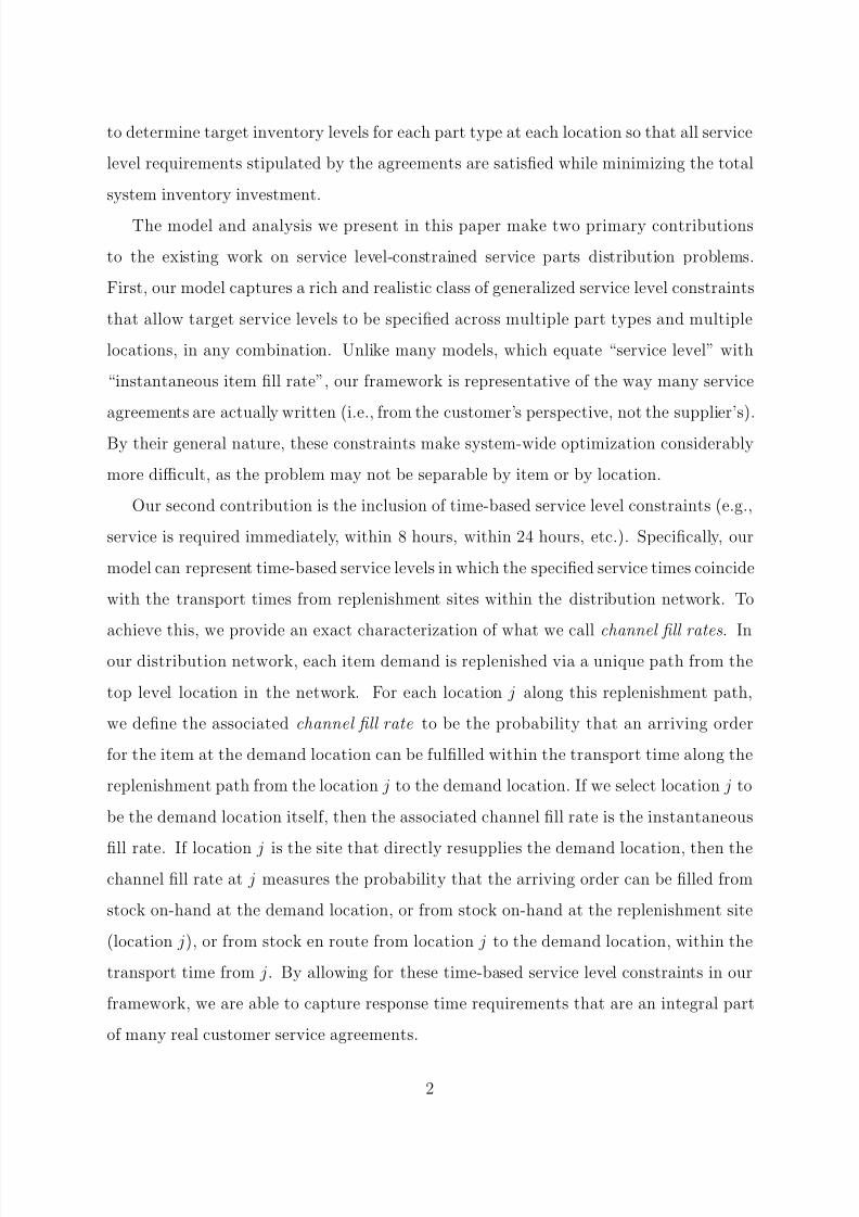
1 Introduction
In the realm of service parts management, customer relationships are often established
through service agreements that extend over a period of months or years. These agree-
ments typically apply to a product (or group of products) that the customer has pur-
chased, and specify the type of service that will be provided, as well as the timing with
which the service will take place. In the case of a customer that operates in multiple
locations, service agreements may apply to several products across several locations.
Examples of product types for which service agreements are common include auto-
mobiles, aircraft, computers, and office equipment. Service is provided on an as-needed
basis and entails the replacement of one or more component parts. As these compo-
nents may vary widely in cost and failure rate, procuring and positioning service parts
throughout the supply chain so that all customer service agreements can be honored in
a cost-effective manner is a considerable challenge.
In meeting this challenge, it is imperative for the supplier to recognize that the cus-
tomer’s concern is the maintenance of the product , not the maintenance of the individual
component parts. This is similar in spirit to Smith et al. (1980) and Cohen et al. (1989).
By understanding the customer’s service level requirements in terms of the product , as
well as the timing with which the customer is willing to receive service, suppliers of
service parts can achieve considerable savings in inventory investment and operational
overhead. One of the goals of this research is to understand how the construction of
such service level agreements impacts the procurement and positioning of service parts
throughout the supply chain.
In this paper we consider a multi-item, multi-echelon distribution system in which
general service level requirements have been established. Locations at the lowest level,
or echelon, of the distribution network experience demand for parts on a continual basis.
The topology of the system is such that each location on a particular level is replenished
from a unique location at the next-higher level over a constant transport lead time. The
location at the top level is replenished via a process that has a known and constant lead
time. Demands that cannot be fulfilled immediately are backordered. The objective is
1
8/3/2019 Industry Study on Parts Management and Ordering Strategy
http://slidepdf.com/reader/full/industry-study-on-parts-management-and-ordering-strategy 5/46
to determine target inventory levels for each part type at each location so that all service
level requirements stipulated by the agreements are satisfied while minimizing the total
system inventory investment.
The model and analysis we present in this paper make two primary contributions
to the existing work on service level-constrained service parts distribution problems.
First, our model captures a rich and realistic class of generalized service level constraints
that allow target service levels to be specified across multiple part types and multiple
locations, in any combination. Unlike many models, which equate “service level” with
“instantaneous item fill rate”, our framework is representative of the way many service
agreements are actually written (i.e., from the customer’s perspective, not the supplier’s).
By their general nature, these constraints make system-wide optimization considerably
more difficult, as the problem may not be separable by item or by location.
Our second contribution is the inclusion of time-based service level constraints (e.g.,
service is required immediately, within 8 hours, within 24 hours, etc.). Specifically, our
model can represent time-based service levels in which the specified service times coincide
with the transport times from replenishment sites within the distribution network. To
achieve this, we provide an exact characterization of what we call channel fill rates. In
our distribution network, each item demand is replenished via a unique path from the
top level location in the network. For each location j along this replenishment path,
we define the associated channel fill rate to be the probability that an arriving order
for the item at the demand location can be fulfilled within the transport time along the
replenishment path from the location j to the demand location. If we select location j to
be the demand location itself, then the associated channel fill rate is the instantaneous
fill rate. If location j is the site that directly resupplies the demand location, then thechannel fill rate at j measures the probability that the arriving order can be filled from
stock on-hand at the demand location, or from stock on-hand at the replenishment site
(location j), or from stock en route from location j to the demand location, within the
transport time from j. By allowing for these time-based service level constraints in our
framework, we are able to capture response time requirements that are an integral part
of many real customer service agreements.
2
8/3/2019 Industry Study on Parts Management and Ordering Strategy
http://slidepdf.com/reader/full/industry-study-on-parts-management-and-ordering-strategy 6/46
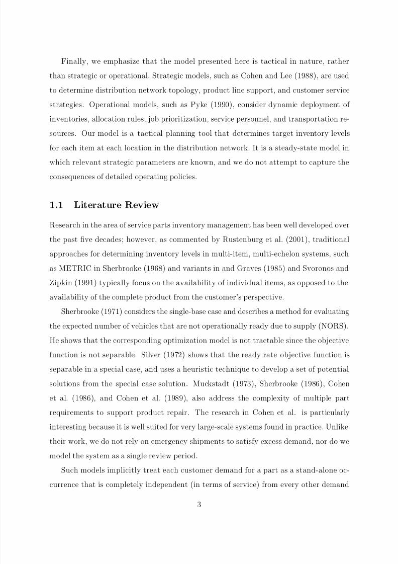
Finally, we emphasize that the model presented here is tactical in nature, rather
than strategic or operational. Strategic models, such as Cohen and Lee (1988), are used
to determine distribution network topology, product line support, and customer service
strategies. Operational models, such as Pyke (1990), consider dynamic deployment of
inventories, allocation rules, job prioritization, service personnel, and transportation re-
sources. Our model is a tactical planning tool that determines target inventory levels
for each item at each location in the distribution network. It is a steady-state model in
which relevant strategic parameters are known, and we do not attempt to capture the
consequences of detailed operating policies.
1.1 Literature Review
Research in the area of service parts inventory management has been well developed over
the past five decades; however, as commented by Rustenburg et al. (2001), traditional
approaches for determining inventory levels in multi-item, multi-echelon systems, such
as METRIC in Sherbrooke (1968) and variants in and Graves (1985) and Svoronos and
Zipkin (1991) typically focus on the availability of individual items, as opposed to the
availability of the complete product from the customer’s perspective.
Sherbrooke (1971) considers the single-base case and describes a method for evaluating
the expected number of vehicles that are not operationally ready due to supply (NORS).
He shows that the corresponding optimization model is not tractable since the objective
function is not separable. Silver (1972) shows that the ready rate objective function is
separable in a special case, and uses a heuristic technique to develop a set of potential
solutions from the special case solution. Muckstadt (1973), Sherbrooke (1986), Cohen
et al. (1986), and Cohen et al. (1989), also address the complexity of multiple part
requirements to support product repair. The research in Cohen et al. is particularly
interesting because it is well suited for very large-scale systems found in practice. Unlike
their work, we do not rely on emergency shipments to satisfy excess demand, nor do we
model the system as a single review period.
Such models implicitly treat each customer demand for a part as a stand-alone oc-
currence that is completely independent (in terms of service) from every other demand
3

8/3/2019 Industry Study on Parts Management and Ordering Strategy
http://slidepdf.com/reader/full/industry-study-on-parts-management-and-ordering-strategy 7/46
made by the same customer. In many circumstances, this is an appropriate model; how-
ever, in an environment where service agreements are prevalent, it clearly is not. While
instantaneous item fill rates are necessary for the computation of service levels in such
an environment, they are not usually, by themselves, the service levels with which the
customers are concerned.
A related body of research is the development of policies for components used in
assembly systems. Smith et al. were the first to introduce the notion of job completion
rate corresponding to the joint probability that all required items are available to complete
a repair or service. Extensions include Mamer and Smith (1982), Graves (1982), Schmidt
and Nahmias (1985), Yano (1987), Cheung and Hausman (1995), Hausman et al. (1998),
Song (1998), Song et al. (1999), and Agrawal and Cohen (2001). As in this research,
we are concerned with the overall service level at the product level, rather than the part
level. Cohen et al. (1989) consider a multiple item stock problem at a single echelon. As
in their research, the demanded items may be considered as consumables or reparables.
Our work differs past research in two important ways. First, our work supports
generalized service level constraints referred to as “contracts,” as is commonly found in
practice. It is our objective to minimize overall system inventory investment while satis-
fying a set of service contracts. These contracts may be quite complex specifying different
supply chain structures, including inventory sharing between locations, for different parts
items. Second, we model the multi-echelon, multi-item system as a continuous review
system. This differs from Cohen et al. (1986) and Cohen et al. (1989) in that we do not
assume that the system is “reset” to some nominal condition at the end of a review pe-
riod. In the spirit of the METRIC approach, inventory levels at upstream locations will
affect the expected replenishment lead times to downstream locations and consequentlywill impact customer fill rates.
The remainder of the paper is organized as follows. In Section 2, we describe our
modeling framework in detail and formulate the problem as a mathematical program. In
Section 3, we derive exact expressions for the channel fill rates that are key to analyzing
the aggregate service level fulfillment. In Section 4 we describe an iterative approxima-
tion scheme for solving the problem. An example problem is examined in Section 5.
4
8/3/2019 Industry Study on Parts Management and Ordering Strategy
http://slidepdf.com/reader/full/industry-study-on-parts-management-and-ordering-strategy 8/46
In Section 6 we describe an approach for constructing an approximate solution vector
that may be used to initialize the algorithm outlined in Section 4. We summarize our
contributions in Section 7.
2 The Model
In this section we state the assumptions upon which our model is based and illustrate the
types of service level requirements that can be represented within the modeling frame-
work. We conclude by defining notation and presenting a mathematical programming
formulation of the problem.
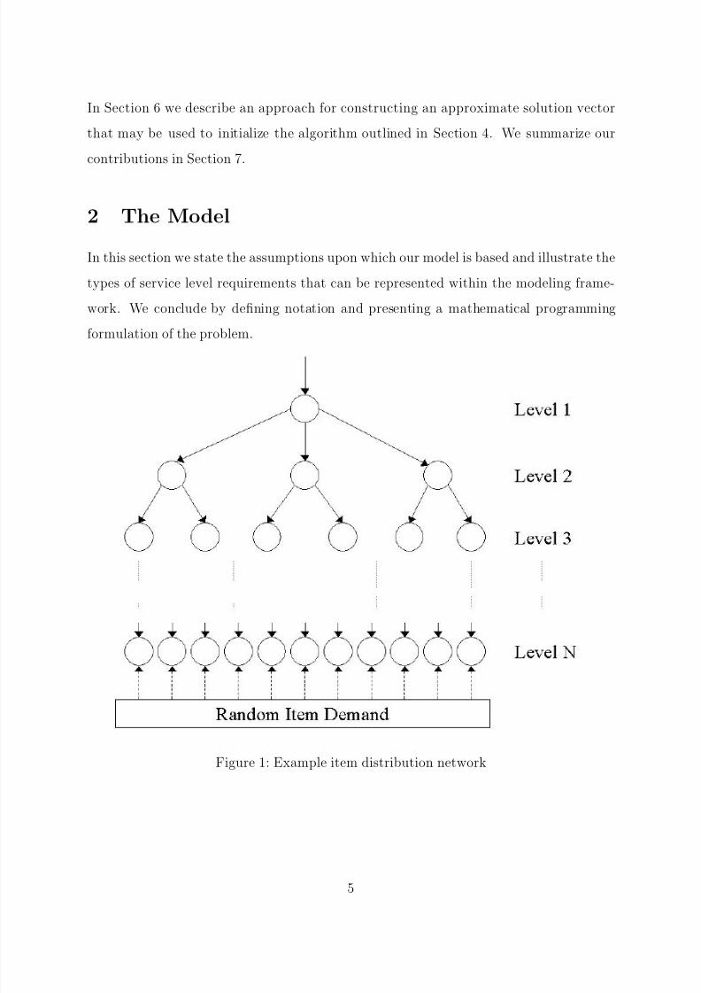
Figure 1: Example item distribution network
5

8/3/2019 Industry Study on Parts Management and Ordering Strategy
http://slidepdf.com/reader/full/industry-study-on-parts-management-and-ordering-strategy 9/46
2.1 Modeling Assumptions
For our purposes, we consider a multi-item, multi-echelon distribution system with the
following properties:
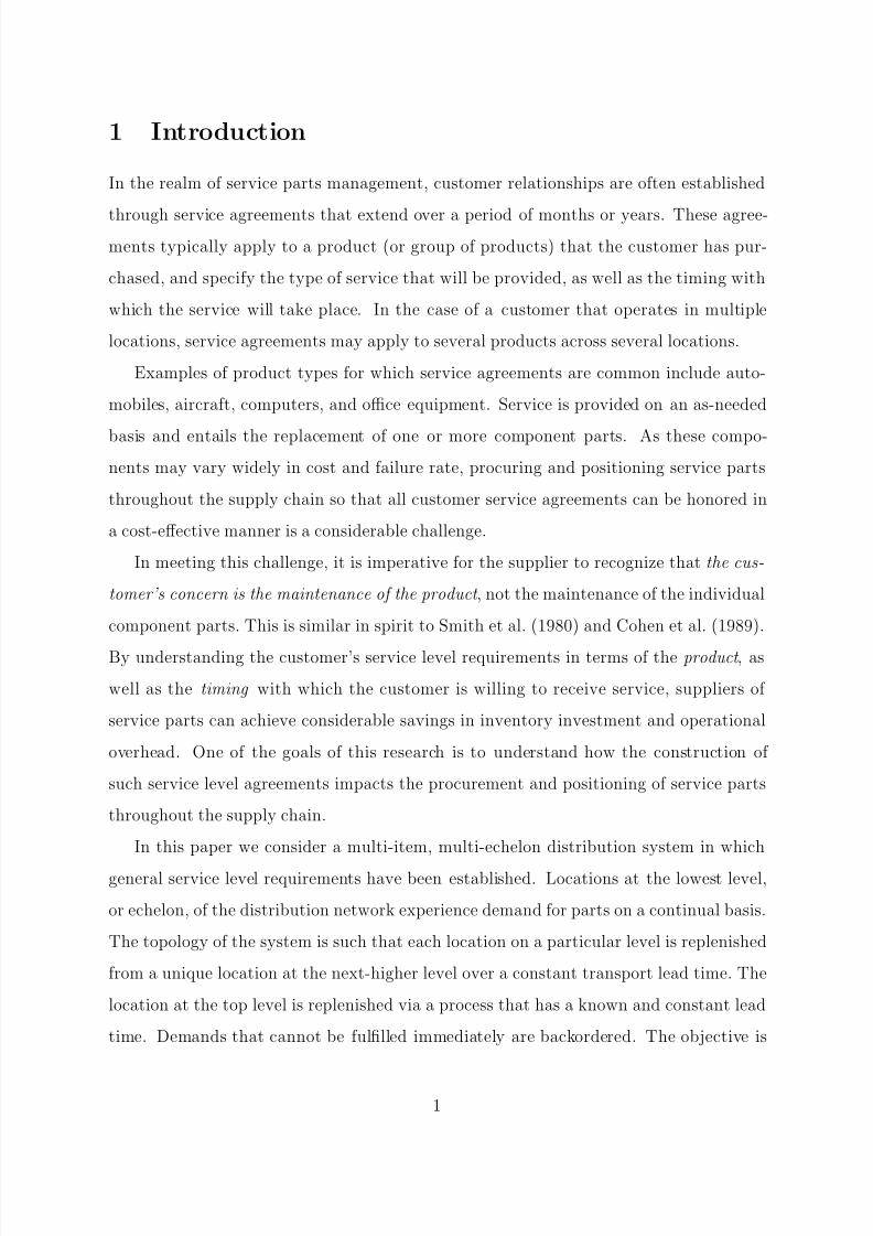
1. The distribution system is the composition of its item distribution networks. Each
item distribution network has a tree-like structure, where each location in the net-
work is replenished from a unique parent location at the next-higher level. The sole
location at the top level of an item network is replenished via a process that has a
known and constant lead time. See Figure 1.
2. Demand for a particular item occurs only at the lowest echelon of the item network.
We refer to locations in the lowest echelon as demand locations. We assume this
without loss of generality, since dummy locations and arcs with negligible lead times
can be added to achieve this structure. In the same manner, we assume that all
demand locations are on the same level in the item distribution network.
3. The demand processes for all items at all demand locations are mutually indepen-
dent Poisson processes with known demand rates. Thus, demands arise for one unit
of an item at a time.
4. All items are replenished on a one-for-one basis at all locations.
5. Transport times for each item between adjacent network locations are known and
constant.
6. Orders that cannot be fulfilled immediately are backordered.
7. Orders are filled at all locations on a first-come, first-serve basis.
For notational convenience only, we assume that all items share a common distribution
network. This will alleviate the need to define a separate network structure for each item.
2.2 Service Level Requirements
We will illustrate the types of service level requirements that may be represented in our
modeling framework with an example.
6

8/3/2019 Industry Study on Parts Management and Ordering Strategy
http://slidepdf.com/reader/full/industry-study-on-parts-management-and-ordering-strategy 10/46
Consider a regional supplier of office equipment whose main business involves leasing
photocopiers. Included in each lease is a service agreement that stipulates the timing
with which equipment breakdowns will be addressed by the supplier. As part of the
agreement, the supplier owns and is responsible for providing any service parts that are
needed to repair malfunctioning equipment.
As it happens, most photocopier breakdowns are caused by worn or overused parts.
Many of these parts, such as toner cartridges, document feed rollers, xerographic mod-
ules, and staples, can be swapped-out quickly and easily, without the aid of a trained
technician. If a breakdown occurs and the needed parts are stocked and available at the
customer location, then repair can commence immediately. If the needed parts are not
available at the customer location, they must be obtained from a regional warehouse.
Parts can be transported from the warehouse to any customer location within 24 hours.
Hence, as long as the needed parts are available either at the customer location or at the
warehouse (or are en- route) at the time a breakdown occurs, the repair can be completed
within a 24-hour time window. Accordingly, the standard service agreement offered by
the supplier is based upon a 24-hour window. Specifically, the agreement stipulates that
all copier breakdowns will be investigated by a service technician within 24 hours, and
that 95% of all copier breakdowns will be fixed within the same period.
Many customers find that the standard service agreement is sufficient to meet their
needs. Some customers, however, depend heavily on the photocopiers and cannot afford
to have their operations disrupted for up to 24 hours on a regular basis. For this second
type of customer, the supplier typically agrees to stock some parts at the customer site
so that a portion of the customer’s breakdowns can be remedied immediately. Recall
that the supplier, not the customer, owns and is responsible for providing the serviceparts. Each time a customer uses a part from their on-site supply to fix a breakdown,
a replacement order is placed immediately with the warehouse. Once the order is filled
at the warehouse, the replacement part will be delivered to the customer site within 24
hours.
There are clearly tradeoffs for the supplier in agreeing to accommodate the second type
of customer. On one hand, stocking parts on-site for a customer will keep the customer
7

8/3/2019 Industry Study on Parts Management and Ordering Strategy
http://slidepdf.com/reader/full/industry-study-on-parts-management-and-ordering-strategy 11/46
satisfied and will result in fewer service calls that require a technician to be dispatched
to that customer site. Also, if the majority of breakdowns require only inexpensive parts
for repair, notable improvements in customer service may be achieved with relatively
little investment. On the other hand, parts that are stocked at the customer site are
not available to service other customer demands. Depending on the demand patterns
and costs of parts and the extent to which customers require instantaneous service, this
could mean a huge investment in service parts inventory in order to honor all service
commitments.
Now consider two offices, a and b, that lease photocopiers from the supplier. These
offices receive service parts from the supplier’s regional warehouse, denoted by r. In office
a, the leased copier is lightly used, and breakdowns are infrequent. Furthermore, when
the copier does break down, alternative means of photocopying are readily available on a
temporary basis. Hence, while office a certainly has no objection to having parts stocked
on-site, the 24-hour service agreement stipulated in the lease is sufficient to meet its
needs. When stock is not on-hand at a, then inventory stocked at r is used to achieve
the desired service level stipulated in the contract.
In office b, however, the leased copier is heavily used, and breakdowns are a regular
occurrence. While a potential 24-hour delay is tolerable once in a great while, frequent
delays of this magnitude would be too disruptive to the operation of the office. Thus, in
addition to the 24-hour service agreement stipulated in the lease, the supplier has agreed
to place enough stock at office b so that 90% of office b’s photocopier breakdowns can be
repaired immediately. Note that this is very different from agreeing to stock the office so
that each photocopier part is immediately available for 90% of all breakdowns in which
the part is required.For purposes of describing the service level constraints associated with the two offices,
we will use the following notation:
• Let I denote the set of photocopier parts, indexed by i.
• Let λa denote the rate at which office a experiences copier breakdowns, and let λia
denote the rate at which office a experiences copier breakdowns that require part i
8
8/3/2019 Industry Study on Parts Management and Ordering Strategy
http://slidepdf.com/reader/full/industry-study-on-parts-management-and-ordering-strategy 12/46
for repair. The ratio λiaλa
then represents the fraction of breakdowns at office a that
require part i for repair. Define λb and λib similarly.
• Let sia and sib denote the stock levels for part i at locations a and b, respectively.Let sir denote the stock level for part i at the regional warehouse r.
• Let f 2ia denote the probability that a breakdown at location a requiring part i can
be fixed immediately. That is, f 2ia is the probability that part i is available on-
site at location a when it is needed. The superscript “2” refers to the level of the
(two-level) network with which the fill rate is associated. Define f 2ib similarly.
• Let f 1ia denote the probability that a breakdown at location a requiring part i can
be filled within 24 hours. That is, f 1ia is the probability that part i is either available
on-site at location a, or it is available at the regional warehouse, or it is en route
from the warehouse to location a when it is needed. Define f 1ib similarly.
The probabilities f 2ia and f 1ia are called channel fill rates for item i at location a, and
we use them as building blocks in constructing service level constraints. Both of these
fill rates are functions of the stock levels sia and sir, although the impact of sir on the
instantaneous fill rate f 2ia is very different from its impact on the 24-hour fill rate f 1ia. We
will explain this difference shortly.
To demonstrate the different types of service level constraints that may arise under
different operating conditions, we present three scenarios.
2.2.1 Scenario 1
In Scenario 1, offices a and b each have their own lease and service agreement with thesupplier, and stock placed on-site at either of the office locations cannot be shared by
the other. Thus, from a distribution viewpoint, offices a and b are distinct stocking
locations. The service level requirements for offices a and b under Scenario 1 are depicted
in Figure 2, and the corresponding constraints are given in 2.1- 2.3.
9

8/3/2019 Industry Study on Parts Management and Ordering Strategy
http://slidepdf.com/reader/full/industry-study-on-parts-management-and-ordering-strategy 13/46
Figure 2: Service Level Requirements for Scenario 1
Constraints 2.1 and 2.2 represent the 24-hour service level guarantees stipulated in the
service agreements for offices a and b, respectively. Constraint 2.3 represents the instan-
taneous service level requirement of office b.
i∈I
λia
λa
f 1ia(sia, sir) ≥ .95, (2.1)
i∈I
λibλb
f 1ib(sib, sir) ≥ .95, (2.2)
i∈I
λibλb
f 2ib(sib, sir) ≥ .90. (2.3)
Note that increasing the stock level sia contributes only to the satisfaction of con-
straint 2.1, and that increasing sib contributes to the satisfaction of 2.2 and 2.3, but not
2.1. This agrees with our intuition, since any stock placed at one of the office locations
cannot be used to service the other, and hence raising the stock level at one office site
should not have any impact on the other office’s service.
By contrast, an increase in sir, the replenishment stock level at the warehouse, con-
tributes to the satisfaction of all three constraints since the fill rates f 1ia, f 1ib, and f 2ib all
depend upon sir. The dependency, however, is different for f 2ib than it is for f 1ia and f 1ib.
Indeed, one may wonder why the instantaneous fill rate f 2ib is affected by the stock level
sir at all. The impact stems from the fact that f 2ib depends in part on the timeliness
10
8/3/2019 Industry Study on Parts Management and Ordering Strategy
http://slidepdf.com/reader/full/industry-study-on-parts-management-and-ordering-strategy 14/46
with which replenishment orders placed by b (to the regional warehouse) are filled , and
this timeliness is fundamentally a function of sir. Having said this, however, it is also
true that sir only affects f 2ib through its impact on the replenishment lead time. Hence,
while it is possible (if sib > 0) to increase the instantaneous fill rate f 2ib by raising the
warehouse stock level sir, there is a limit to the increase that can be achieved by this
method. Beyond this limit, the only way to increase f 2ib is to increase the local stock level
sib. For the 24-hour fill rates f 1ia and f 1ib, there is no such limitation. That is, for any
> 0, it is possible to achieve f 1ia ≥ 1 − (and/or f 1ib ≥ 1 − ) by raising the stock level
sir high enough. We will support these statements mathematically in Section 3, when
we derive explicit characterizations for channel fill rates.
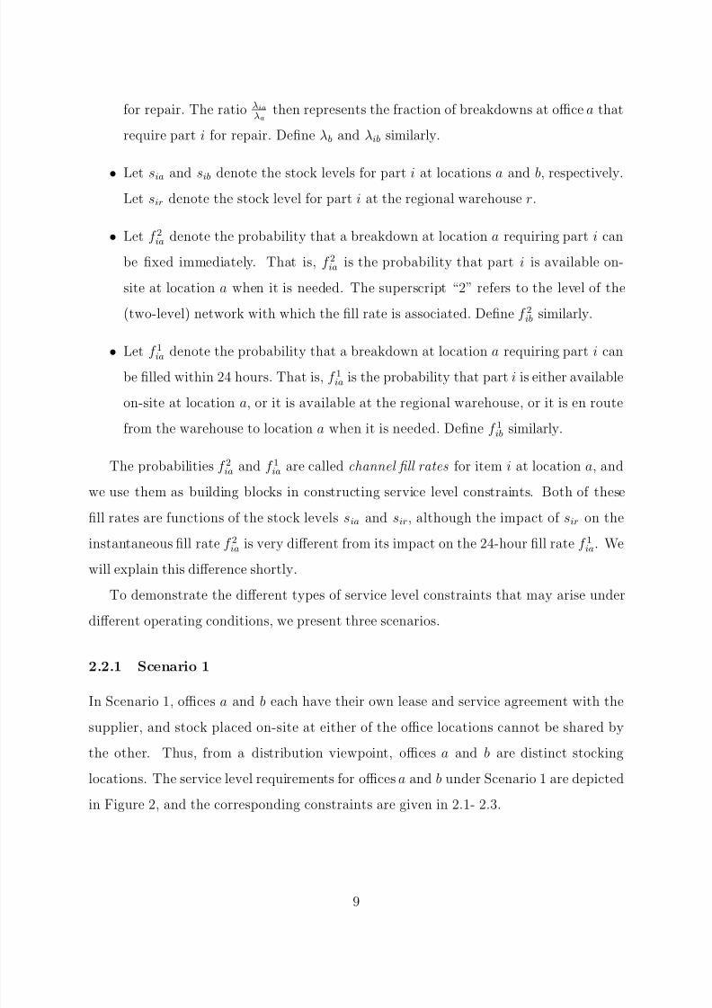
2.2.2 Scenario 2
In Scenario 2, offices a and b each have their own lease and service agreement with the
supplier, but stock placed on-site at either office location can be shared. That is, from
a distribution viewpoint, there is a single stocking location from which offices a and b
draw needed parts. The service level requirements for offices a and b under Scenario 2
are depicted in Figure 3. In the corresponding constraints 2.4- 2.6, ab is used to denotethe common stocking location for offices a and b.
Figure 3: Service Level Requirements for Scenario 2
11
8/3/2019 Industry Study on Parts Management and Ordering Strategy
http://slidepdf.com/reader/full/industry-study-on-parts-management-and-ordering-strategy 15/46
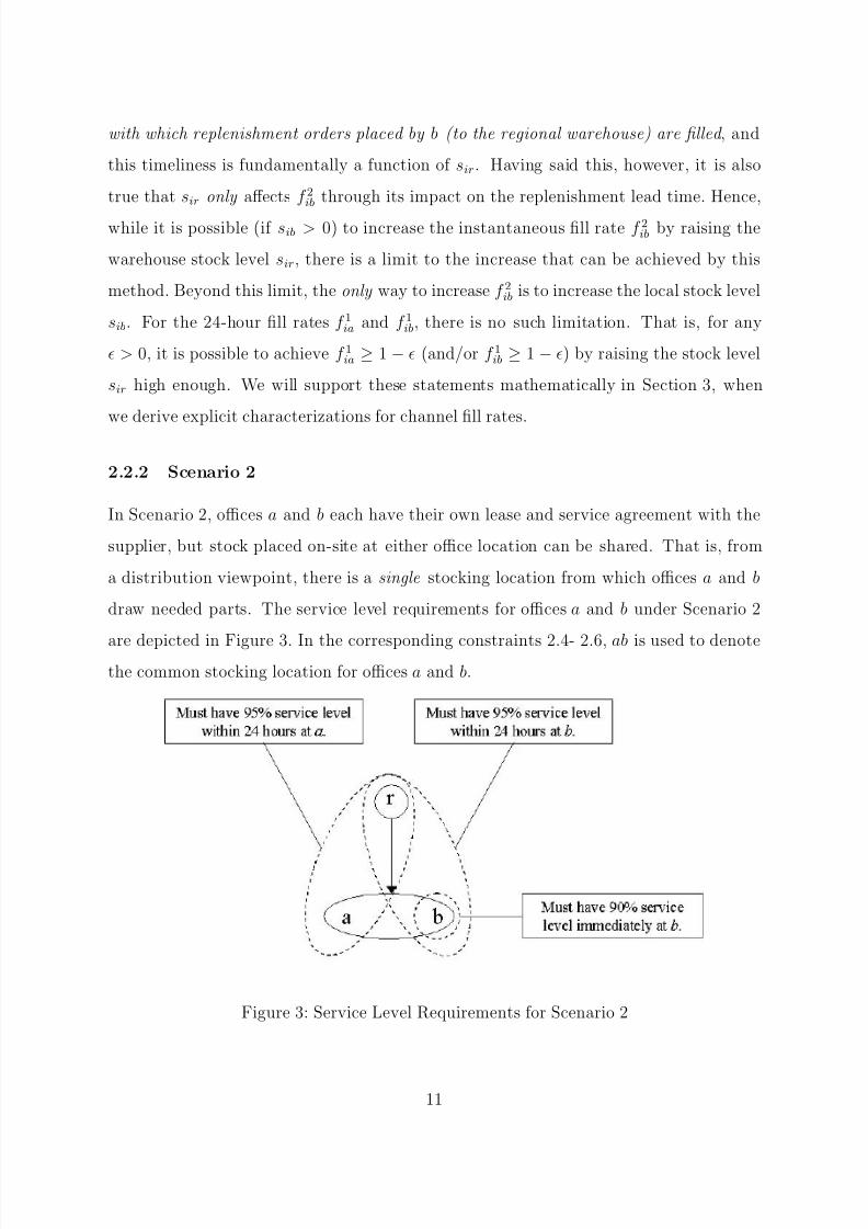
i∈I λiaλa
f 1iab
(siab, sir) ≥ .95, (2.4)
i∈I
λibλb
f 1iab
(siab, sir) ≥ .95, (2.5)
i∈I
λibλb
f 2iab
(siab, sir) ≥ .90. (2.6)
Note that the fill rates and stock levels are indexed by item and stocking location,
not item and customer location. In this case, increasing the stock level siab contributes
to the satisfaction of all three constraints, as we would expect. At first glance, one
might think that the common stocking location makes the constraints in this scenarioa relaxed version of the constraints in Scenario 1. That is, one might suppose that any
stock levels that satisfied 2.1-2.3 would also satisfy 2.4-2.6 if we make the substitution
siab = sia+ sib. In fact, this is not the case for any of the constraints. This is most easily
seen for constraint 2.6.
In Scenario 2, office a will draw stock from location ab to fix its breakdowns (provided
the stock is available), even though it has no instantaneous service level requirement. The
presence of the common stocking location makes the instantaneous fill rate f 2iab a function
of both λia and λib. As a consequence, the satisfaction of constraint 2.6 depends upon the
part demand rates at office a, even though the instantaneous service level requirement
exists at office b only. In order to satisfy 2.6, enough stock must be held at location ab
to make the fill rates f 2iab
, i ∈ I , sufficiently high. A high demand rate λia (relative to
λib) means that siab may have to be significantly higher than Scenario 1’s sib in order for
the fill rate f 2iab
to be as high as Scenario 1’s f 2ib.
This scenario highlights the fact that strategic decisions, such as the placement of
stocking locations, can greatly affect the types of service agreements that can be satisfied
by a supplier in a cost-effective manner. We have just seen that promising a high level of
service to a low-demand customer that draws stock from a high-demand stocking location
can be costly. Since suppliers cannot always avoid such situations, it is important to es-
tablish operating policies that are designed to help achieve the promised customer service
levels. For instance, careful prioritization of customer orders and replenishment orders,
12
8/3/2019 Industry Study on Parts Management and Ordering Strategy
http://slidepdf.com/reader/full/industry-study-on-parts-management-and-ordering-strategy 16/46
as opposed to a simple first-come-first-serve scheme, can improve system performance.
Although we do not address these issues here, research is currently underway to examine
various real-time allocation rules and evaluate their effects on system performance.
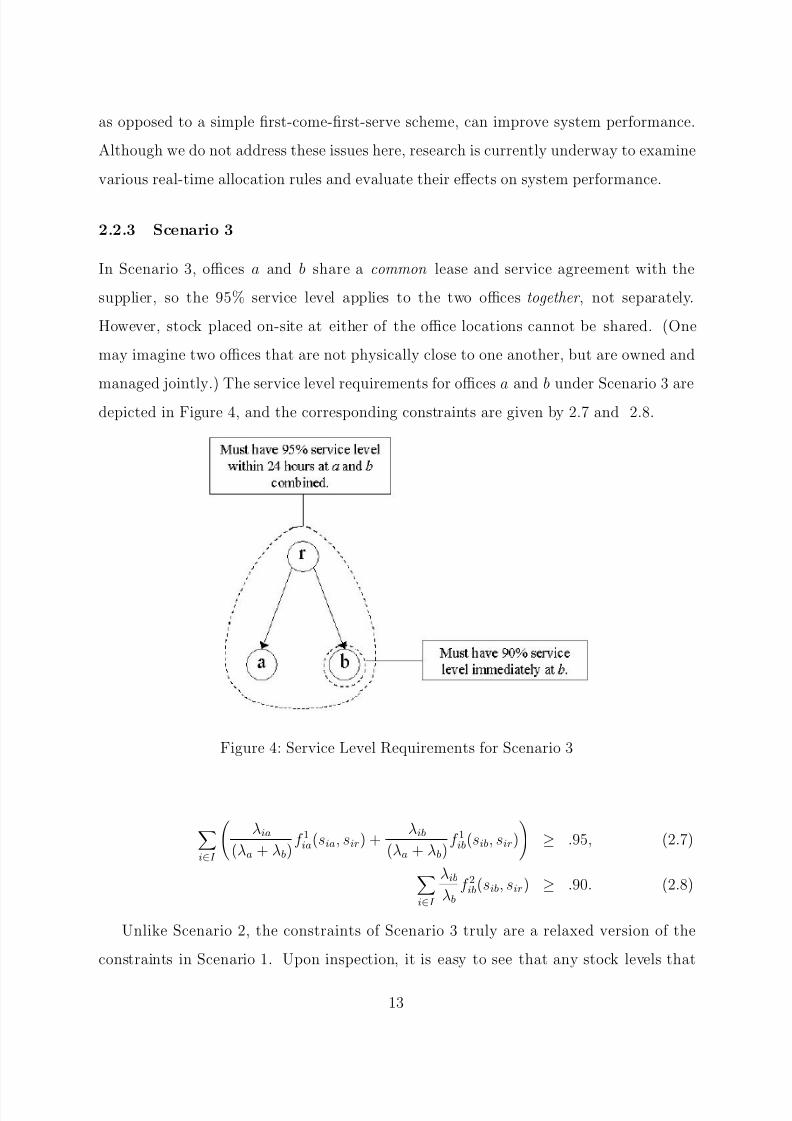
2.2.3 Scenario 3
In Scenario 3, offices a and b share a common lease and service agreement with the
supplier, so the 95% service level applies to the two offices together , not separately.
However, stock placed on-site at either of the office locations cannot be shared. (One
may imagine two offices that are not physically close to one another, but are owned and
managed jointly.) The service level requirements for offices a and b under Scenario 3 are
depicted in Figure 4, and the corresponding constraints are given by 2.7 and 2.8.
Figure 4: Service Level Requirements for Scenario 3
i∈I
λia
(λa + λb)f 1ia(sia, sir) +
λib(λa + λb)
f 1ib(sib, sir)
≥ .95, (2.7)
i∈I
λibλb
f 2ib(sib, sir) ≥ .90. (2.8)
Unlike Scenario 2, the constraints of Scenario 3 truly are a relaxed version of the
constraints in Scenario 1. Upon inspection, it is easy to see that any stock levels that
13
8/3/2019 Industry Study on Parts Management and Ordering Strategy
http://slidepdf.com/reader/full/industry-study-on-parts-management-and-ordering-strategy 17/46
satisfy 2.1-2.3 will also satisfy 2.7 and 2.8. The common service agreement provides the
supplier more flexibility than Scenario 1 in fulfilling the service level requirements.
The preceding scenarios depicted examples of the types of constraints that may be
considered within the framework of our model. In the following subsection we define
notation for the general form of the problem and present the problem as a mathematical
program.
2.3 Notation and Problem Statement
For the remainder of the paper, we will use the following notation:
Distribution Network Parameters
I - the set of items, indexed by i.
J - the set of locations, indexed by j.
J v - the set of locations at level v, v = 1, 2,...,N .N v=1 J v = J ,
and J v1
J v2 = ∅, v1 = v2.
P j - the set of locations in the unique path from location j to the top level
location in the distribution network, inclusive.
P j(v) - the unique location in P j at level v.
p( j) - the parent location of location j in the distribution network, j /∈ J 1.
T ij - the transport time for item i from location p( j) to location j.
τ ij - the expected replenishment lead time for item i from location p( j)
to location j.
ci - the unit investment cost of item i.
Service Level Requirement Parameters
K - the set of service level constraints, indexed by k.
F k - the established service level of service level constraint k.
λij - the rate at which orders for item i arrive at location j.
λijk - the rate at which orders for item i that are associated with service level
constraint k arrive at location j.
14

8/3/2019 Industry Study on Parts Management and Ordering Strategy
http://slidepdf.com/reader/full/industry-study-on-parts-management-and-ordering-strategy 18/46
λk - the total rate at which orders for service parts associated with service
level constraint k are placed. That is, λk =i∈I,j∈J N λijk .
wijk - λijk/λk, the fraction of orders for service parts associated with service
level constraint k that are for item i at location j ∈ J N .
vijk - the level of the distribution network with which service level constraint k
is concerned for item i at location j ∈ J N . vijk ∈ {1, 2,...,N }.
wvijk - the relative weight of channel fill rate f vij in service level constraint k.
That is, wvijk = wijk for v = vijk , and wvijk = 0 otherwise.
Stock Levels and Fill Ratessij - the stock level of item i at location j.
siP j- the vector of stock levels of item i at the locations in P j.
f vij(siP j)- the probability that an incoming order for item i at location j ∈ J N can be
filled within the transport time from location P j(v).
Given the defined notation, we state the Service Level Satisfaction problem, or (SLS)
as:
(SLS) minimizei∈I
j∈J
cisij (2.9)
subject toN v=1
i∈I
j∈J N
wvijkf vij(siP j) ≥ F k ∀k ∈ K, (2.10)
sij ≥ 0 and integer ∀i ∈ I, j ∈ J. (2.11)
There are two sources of complexity in the service level constraints 2.10. The first
is that each fill rate function f vij may appear in multiple service level constraints in
combination with other fill rate functions, so the constraint set may not be separable.
The second source of complexity is the fill rate functions themselves. For a given item i
and a given location j ∈ J N , each channel fill rate f vij, v = 1,...,N , depends in a highly
nonlinear way on the N stock level variables sij , j ∈ P j, as we will now show.
15
8/3/2019 Industry Study on Parts Management and Ordering Strategy
http://slidepdf.com/reader/full/industry-study-on-parts-management-and-ordering-strategy 19/46
3 Channel Fill Rate Functions
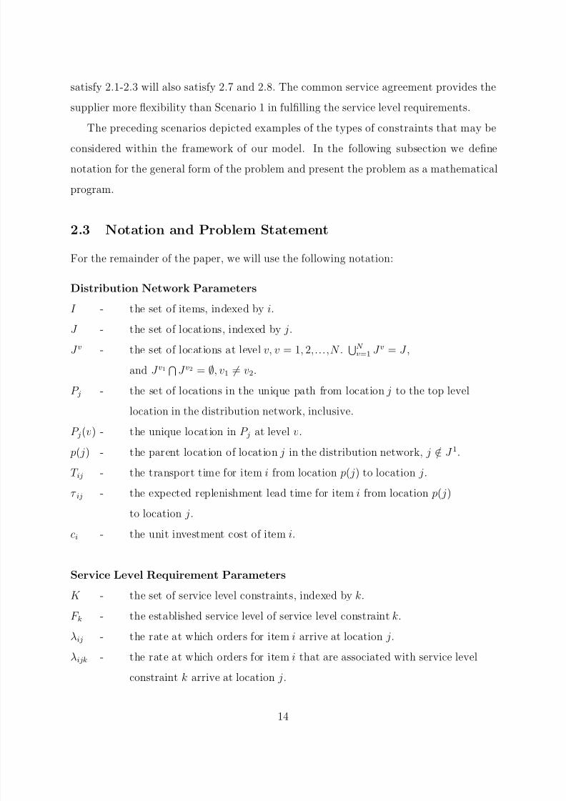
For ease of exposition, we will focus on deriving channel fill rates in a three-level system,
although the analysis extends easily to systems with more than three levels.
Consider a particular item i in the channel composed of locations 1, 2, and 3 in the
distribution network, as shown in Figure 5. Location 3 is the demand location for which
we will explicitly derive the probability expressions for the channel fill rates. Let location
a represent all locations that are replenished by location 1 except for location 2, and let
location b represent all locations replenished by location 2 except for location 3.
Figure 5: Item distribution network
For notational clarity, we will suppress the i subscript on all variables and parameters.
The following variable definitions will be helpful in our discussion. Let:
Y j - the number of units on order at location j, j = 1, 2, 3, a , b.
N j - [Y j − s j ]+, the number of units backordered at location j, j = 1, 2, 3, a , b.
E j - the number of units en route from location p( j) to location j, j = 2, 3, a , b.
16
8/3/2019 Industry Study on Parts Management and Ordering Strategy
http://slidepdf.com/reader/full/industry-study-on-parts-management-and-ordering-strategy 20/46
Z j - (Y j − E j), the number of units on order at location j that are still
backordered at location p( j), j = 2, 3, a , b. This also represents the
number of units currently on order at location j that will not arrive at
location j within T j units of time.
Our goal in this section is to provide exact expressions for the channel fill rates at
location 3 in terms of the probability distributions of Y 1, Y 2, and Y 3. Although the
distributions of Y 1, Y 2, and Y 3 are difficult to characterize exactly, for given stock levels
(s1, s2, s3) and transport times (T 1, T 2, T 3), the means and variances can be easily
calculated. Thus, using ideas from Graves (1985), we can approximate the distributions
of Y 1, Y 2, and Y 3 with negative binomial distributions having these means and variances.
Combining these results yields a mechanism for evaluating the service level constraints
2.10 presented in the previous section.
3.1 The fill rate f 33 (s3, s2, s1)
We begin with f 33 (s3, s2, s1), since this is the simplest case. In the context of our network,
f 3
3 (s3, s2, s1) is the probability that an incoming order (for item i) at location 3 can befilled immediately. An instantaneous fill can occur if and only if there is stock on-hand
at location 3 when the order arrives. Since a one-for-one replenishment policy is followed
in the network, this is equivalent to having strictly less than s3 units on order at location
3 at the time the new order arrives. Hence,
f 33 (s3, s2, s1) = Pr[Y 3 < s3]. (3.1)
When s3 = 0, the instantaneous fill rate is also 0, as we would expect.
Although we have not made any explicit statements yet about the distribution of Y 3,
we can easily derive an upper bound for f 33 . Note that the distribution of Y 3 depends only
on the demand process at location 3 and the order replenishment lead time at location
3. That is, Y 3 is a function of s2, and s1, but not s3. For finite values of s2, it is clear
that the distribution function of Y 3 is monotonically increasing in s2. When s2 = ∞, the
replenishment lead time for location 3 is exactly the transport time T 3. In this case, a
17

8/3/2019 Industry Study on Parts Management and Ordering Strategy
http://slidepdf.com/reader/full/industry-study-on-parts-management-and-ordering-strategy 21/46
well-known result of Feeney and Sherbrooke (1966) gives us that Y 3 is a Poisson random
variable with mean λ3T 3. Hence, for any values of s2 and s1, we have that:
Pr[Y 3 < s3] ≤
s3−1x=0
(λ3T 3)xe−λ3T 3
x! . (3.2)
This supports our earlier claim that there is a limit to the impact that increasing s2
can have on f 33 . Indeed, increasing s2 will tend to drive the distribution of Y 3 towards a
Poisson distribution with mean λ3T 3, but this is the extent of its impact on f 33 . In general,
Y 3 will have a distribution with mean λ3τ 3, where τ 3 denotes the expected replenishment
lead time. It is always the case that τ 3 ≥ T 3.
3.2 The fill rate f 23 (s3, s2, s1)
Next, let us determine the probability that an incoming order at location 3 can be filled
within time T 3, the transport time from location 2 to location 3. We will consider two
cases: s3 = 0; and s3 > 0.
When s3 = 0, all orders arriving at location 3 effectively are filled from stock at
location 2. That is, each order that arrives at location 3 waits at least T 3 units of time
until it is filled, since there is never any stock on-hand at location 3, and any units en-route from location 2 to location 3 at the time an order arrives are already claimed by
existing backorders at location 3. Hence, a new order arriving at location 3 will be filled
within T 3 units of time if and only if there is stock on-hand at location 2 when the order
arrives. That is,
f 23 (s3, s2, s1) = Pr[Y 2 < s2], if s3 = 0. (3.3)
Observe that this fill rate will be 0 when s2 = s3 = 0.
Now consider the case where s3 > 0. Recall that Z 3 represents the number of units
currently on order at location 3 that will not arrive at location 3 within T 3 units of time.
Hence, a newly arriving order to location 3 will be filled within T 3 units of time if and
only if Z 3 < s3. That is:
f 23 (s3, s2, s1) = Pr[Z 3 < s3] , if s3 > 0. (3.4)
18
8/3/2019 Industry Study on Parts Management and Ordering Strategy
http://slidepdf.com/reader/full/industry-study-on-parts-management-and-ordering-strategy 22/46
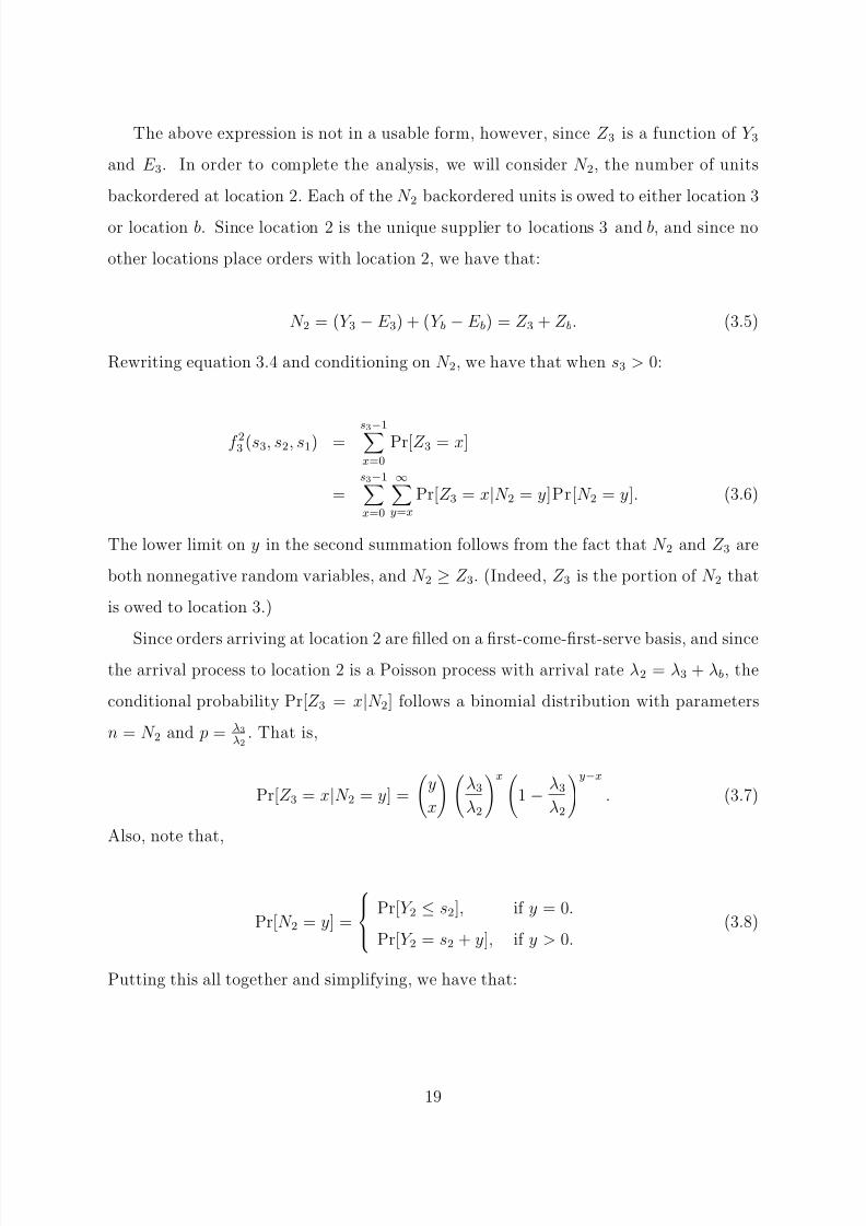
The above expression is not in a usable form, however, since Z 3 is a function of Y 3
and E 3. In order to complete the analysis, we will consider N 2, the number of units
backordered at location 2. Each of the N 2 backordered units is owed to either location 3
or location b. Since location 2 is the unique supplier to locations 3 and b, and since no
other locations place orders with location 2, we have that:
N 2 = (Y 3 − E 3) + (Y b − E b) = Z 3 + Z b. (3.5)
Rewriting equation 3.4 and conditioning on N 2, we have that when s3 > 0:
f 23 (s3, s2, s1) =s3−1x=0
Pr[Z 3 = x]
=s3−1x=0
∞y=x
Pr[Z 3 = x|N 2 = y]Pr[N 2 = y]. (3.6)
The lower limit on y in the second summation follows from the fact that N 2 and Z 3 are
both nonnegative random variables, and N 2 ≥ Z 3. (Indeed, Z 3 is the portion of N 2 that
is owed to location 3.)
Since orders arriving at location 2 are filled on a first-come-first-serve basis, and sincethe arrival process to location 2 is a Poisson process with arrival rate λ2 = λ3 + λb, the
conditional probability Pr[Z 3 = x|N 2] follows a binomial distribution with parameters
n = N 2 and p = λ3λ2
. That is,
Pr[Z 3 = x|N 2 = y] =
y
x
λ3
λ2
x 1 −
λ3
λ2
y−x. (3.7)
Also, note that,
Pr[N 2 = y] =
Pr[Y 2 ≤ s2], if y = 0.
Pr[Y 2 = s2 + y], if y > 0.(3.8)
Putting this all together and simplifying, we have that:
19
8/3/2019 Industry Study on Parts Management and Ordering Strategy
http://slidepdf.com/reader/full/industry-study-on-parts-management-and-ordering-strategy 23/46
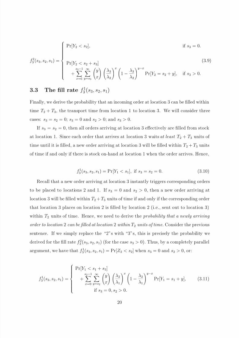
f 23 (s3, s2, s1) =
Pr[Y 2 < s2], if s3 = 0.
Pr[Y 2 < s2 + s3]
+s3−1x=0
∞y=s3
y
x
λ3
λ2
x 1 −
λ3
λ2
y−xPr[Y 2 = s2 + y], if s3 > 0.
(3.9)
3.3 The fill rate f 13 (s3, s2, s1)
Finally, we derive the probability that an incoming order at location 3 can be filled within
time T 2 + T 3, the transport time from location 1 to location 3. We will consider three
cases: s3 = s2 = 0; s3 = 0 and s2 > 0; and s3 > 0.
If s3 = s2 = 0, then all orders arriving at location 3 effectively are filled from stock
at location 1. Since each order that arrives at location 3 waits at least T 2 + T 3 units of
time until it is filled, a new order arriving at location 3 will be filled within T 2 + T 3 units
of time if and only if there is stock on-hand at location 1 when the order arrives. Hence,
f 13 (s3, s2, s1) = Pr[Y 1 < s1], if s3 = s2 = 0. (3.10)
Recall that a new order arriving at location 3 instantly triggers corresponding orders
to be placed to locations 2 and 1. If s3 = 0 and s2 > 0, then a new order arriving at
location 3 will be filled within T 2 + T 3 units of time if and only if the corresponding order
that location 3 places on location 2 is filled by location 2 (i.e., sent out to location 3)
within T 2 units of time. Hence, we need to derive the probability that a newly arriving
order to location 2 can be filled at location 2 within T 2 units of time. Consider the previous
sentence. If we simply replace the “2”s with “3”s, this is precisely the probability we
derived for the fill rate f 23 (s3, s2, s1) (for the case s3 > 0). Thus, by a completely parallel
argument, we have that f 13 (s3, s2, s1) = Pr[Z 2 < s2] when s3 = 0 and s2 > 0, or:
f 13 (s3, s2, s1) =
Pr[Y 1 < s1 + s2]
+s2−1x=0
∞y=s2
y
x
λ2
λ1
x 1 −
λ2
λ1
y−xPr[Y 1 = s1 + y],
if s3 = 0, s2 > 0.
(3.11)
20
8/3/2019 Industry Study on Parts Management and Ordering Strategy
http://slidepdf.com/reader/full/industry-study-on-parts-management-and-ordering-strategy 24/46
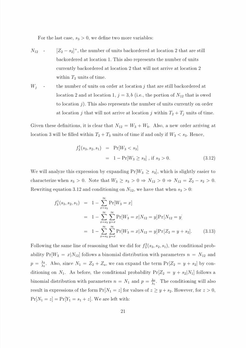
For the last case, s3 > 0, we define two more variables:
N 12 - [Z 2 − s2]+, the number of units backordered at location 2 that are still
backordered at location 1. This also represents the number of unitscurrently backordered at location 2 that will not arrive at location 2
within T 2 units of time.
W j - the number of units on order at location j that are still backordered at
location 2 and at location 1, j = 3, b (i.e., the portion of N 12 that is owed
to location j). This also represents the number of units currently on order
at location j that will not arrive at location j within T 2 + T j units of time.
Given these definitions, it is clear that N 12 = W 3 + W b. Also, a new order arriving at
location 3 will be filled within T 2 + T 3 units of time if and only if W 3 < s3. Hence,
f 13 (s3, s2, s1) = Pr[W 3 < s3]
= 1 − Pr[W 3 ≥ s3] , if s3 > 0. (3.12)
We will analyze this expression by expanding Pr[W 3 ≥ s3], which is slightly easier to
characterize when s3 > 0. Note that W 3 ≥ s3 > 0 ⇒ N 12 > 0 ⇒ N 12 = Z 2 − s2 > 0.Rewriting equation 3.12 and conditioning on N 12, we have that when s3 > 0:
f 13 (s3, s2, s1) = 1 −∞x=s3
Pr[W 3 = x]
= 1 −∞x=s3
∞y=x
Pr[W 3 = x|N 12 = y]Pr[N 12 = y]
= 1 −∞x=s3
∞y=x
Pr[W 3 = x|N 12 = y]Pr[Z 2 = y + s2]. (3.13)
Following the same line of reasoning that we did for f 23 (s3, s2, s1), the conditional prob-
ability Pr[W 3 = x|N 12] follows a binomial distribution with parameters n = N 12 and
p = λ3λ2
. Also, since N 1 = Z 2 + Z a, we can expand the term Pr[Z 2 = y + s2] by con-
ditioning on N 1. As before, the conditional probability Pr[Z 2 = y + s2|N 1] follows a
binomial distribution with parameters n = N 1 and p = λ2λ1
. The conditioning will also
result in expressions of the form Pr[N 1 = z] for values of z ≥ y + s2. However, for z > 0,
Pr[N 1 = z] = Pr[Y 1 = s1 + z]. We are left with:
21
8/3/2019 Industry Study on Parts Management and Ordering Strategy
http://slidepdf.com/reader/full/industry-study-on-parts-management-and-ordering-strategy 25/46
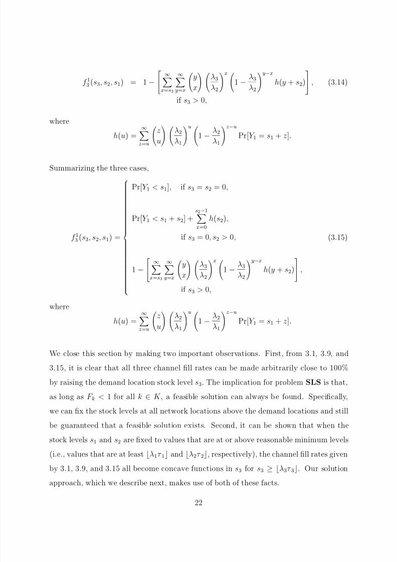
f 13 (s3, s2, s1) = 1 −
∞x=s3
∞y=x
y
x
λ3
λ2
x 1 −
λ3
λ2
y−xh(y + s2)
, (3.14)
if s3 > 0,
where
h(u) =∞z=u
z
u
λ2
λ1
u 1 −
λ2
λ1
z−uPr[Y 1 = s1 + z].
Summarizing the three cases,
f 13 (s3, s2, s1) =
Pr[Y 1 < s1], if s3 = s2 = 0,
Pr[Y 1 < s1 + s2] +s2−1x=0
h(s2),
if s3 = 0, s2 > 0,
1 −
∞x=s3
∞y=x
y
x
λ3
λ2
x 1 −
λ3
λ2
y−xh(y + s2)
,
if s3 > 0,
(3.15)
where
h(u) =∞z=u
z
u
λ2
λ1
u 1 −
λ2
λ1
z−uPr[Y 1 = s1 + z].
We close this section by making two important observations. First, from 3.1, 3.9, and
3.15, it is clear that all three channel fill rates can be made arbitrarily close to 100%
by raising the demand location stock level s3. The implication for problem SLS is that,
as long as F k < 1 for all k ∈ K , a feasible solution can always be found. Specifically,
we can fix the stock levels at all network locations above the demand locations and still
be guaranteed that a feasible solution exists. Second, it can be shown that when the
stock levels s1 and s2 are fixed to values that are at or above reasonable minimum levels
(i.e., values that are at least λ1τ 1 and λ2τ 2, respectively), the channel fill rates given
by 3.1, 3.9, and 3.15 all become concave functions in s3 for s3 ≥ λ3τ 3. Our solution
approach, which we describe next, makes use of both of these facts.
22
8/3/2019 Industry Study on Parts Management and Ordering Strategy
http://slidepdf.com/reader/full/industry-study-on-parts-management-and-ordering-strategy 26/46
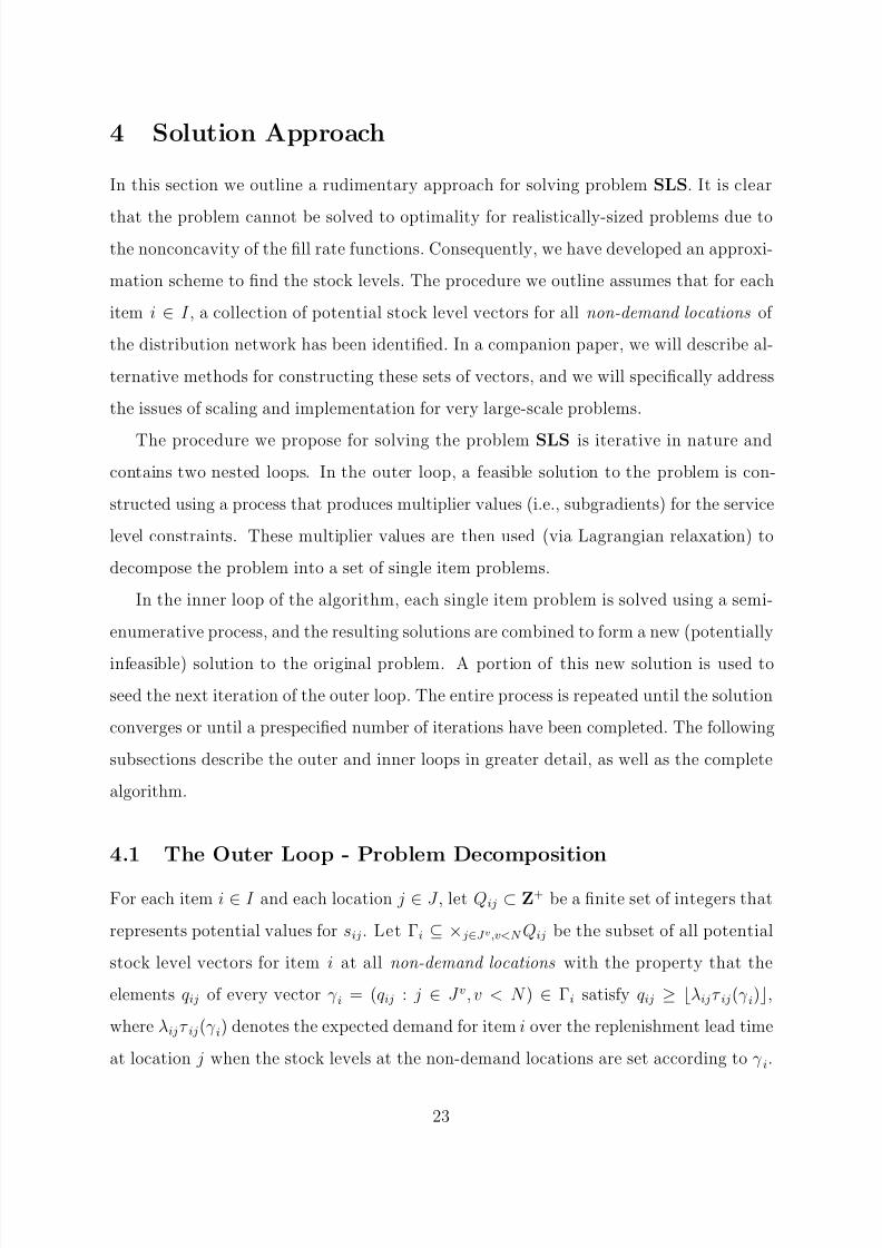
4 Solution Approach
In this section we outline a rudimentary approach for solving problem SLS. It is clear
that the problem cannot be solved to optimality for realistically-sized problems due to
the nonconcavity of the fill rate functions. Consequently, we have developed an approxi-
mation scheme to find the stock levels. The procedure we outline assumes that for each
item i ∈ I , a collection of potential stock level vectors for all non-demand locations of
the distribution network has been identified. In a companion paper, we will describe al-
ternative methods for constructing these sets of vectors, and we will specifically address
the issues of scaling and implementation for very large-scale problems.
The procedure we propose for solving the problem SLS is iterative in nature and
contains two nested loops. In the outer loop, a feasible solution to the problem is con-
structed using a process that produces multiplier values (i.e., subgradients) for the service
level constraints. These multiplier values are then used (via Lagrangian relaxation) to
decompose the problem into a set of single item problems.
In the inner loop of the algorithm, each single item problem is solved using a semi-
enumerative process, and the resulting solutions are combined to form a new (potentially
infeasible) solution to the original problem. A portion of this new solution is used to
seed the next iteration of the outer loop. The entire process is repeated until the solution
converges or until a prespecified number of iterations have been completed. The following
subsections describe the outer and inner loops in greater detail, as well as the complete
algorithm.
4.1 The Outer Loop - Problem Decomposition
For each item i ∈ I and each location j ∈ J , let Qij ⊂ Z+ be a finite set of integers that
represents potential values for sij. Let Γi ⊆ × j∈J v,v<N Qij be the subset of all potential
stock level vectors for item i at all non-demand locations with the property that the
elements qij of every vector γ i = (qij : j ∈ J v, v < N ) ∈ Γi satisfy qij ≥ λijτ ij(γ i),
where λijτ ij(γ i) denotes the expected demand for item i over the replenishment lead time
at location j when the stock levels at the non-demand locations are set according to γ i.
23
8/3/2019 Industry Study on Parts Management and Ordering Strategy
http://slidepdf.com/reader/full/industry-study-on-parts-management-and-ordering-strategy 27/46
That is, we want to restrict ourselves to vectors of stock levels that are jointly reasonable
from a practical standpoint.
We noted earlier that the functions f vij(·) are not concave in their arguments jointly.
However, observe what happens to SLS when for every item i ∈ I , we fix the stock levels
sij at all non-demand locations to values given by a vector γ i = (qij : j ∈ J v, v < N ) ∈ Γi.
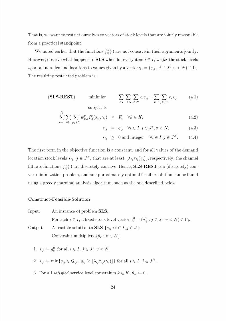
The resulting restricted problem is:
(SLS-REST) minimizei∈I
v<N
j∈J v
cisij +i∈I
j∈J N
cisij (4.1)
subject to
N v=1
i∈I
j∈J N
wvijkf vij(sij, γ i) ≥ F k ∀k ∈ K, (4.2)
sij = qij ∀i ∈ I, j ∈ J v, v < N, (4.3)
sij ≥ 0 and integer ∀i ∈ I, j ∈ J N . (4.4)
The first term in the objective function is a constant, and for all values of the demand
location stock levels sij, j ∈ J N , that are at least λijτ ij(γ i), respectively, the channel
fill rate functions f
v
ij(·) are discretely concave. Hence, SLS-REST is a (discretely) con-vex minimization problem, and an approximately optimal feasible solution can be found
using a greedy marginal analysis algorithm, such as the one described below.
Construct-Feasible-Solution
Input: An instance of problem SLS;
For each i ∈ I , a fixed stock level vector γ 0i = (q0ij : j ∈ J v, v < N ) ∈ Γi.
Output: A feasible solution to SLS {sij : i ∈ I, j ∈ J };
Constraint multipliers {θk : k ∈ K }.
1. sij ← q0ij for all i ∈ I , j ∈ J v, v < N .
2. sij ← min{qij ∈ Qij : qij ≥ λijτ ij(γ i)} for all i ∈ I , j ∈ J N .
3. For all satisfied service level constraints k ∈ K , θk ← 0.
24
8/3/2019 Industry Study on Parts Management and Ordering Strategy
http://slidepdf.com/reader/full/industry-study-on-parts-management-and-ordering-strategy 28/46
4. For all unsatisfied service level constraints k ∈ K , and all i ∈ I, j ∈ J N , compute:
∆ijk = min{F k,N
v=1wvijkf vij(sij + 1, γ i)} −
N
v=1wvijkf vij(sij, γ i).
5. Find the triplet (i,j,k)∗ such that:
(i,j,k)∗ = arg max(i,j,k)
∆ijkci
.
6. If N v=1
w∗vijkf ∗vij (s∗ij + 1, γ i) ≥ F ∗k , then θk ←
∆∗
ijk
c∗i
.
7. s∗ij ← s∗ij + 1.
8. If all service level constraints k ∈ K are satisfied, then STOP. Otherwise, go to
step 4.
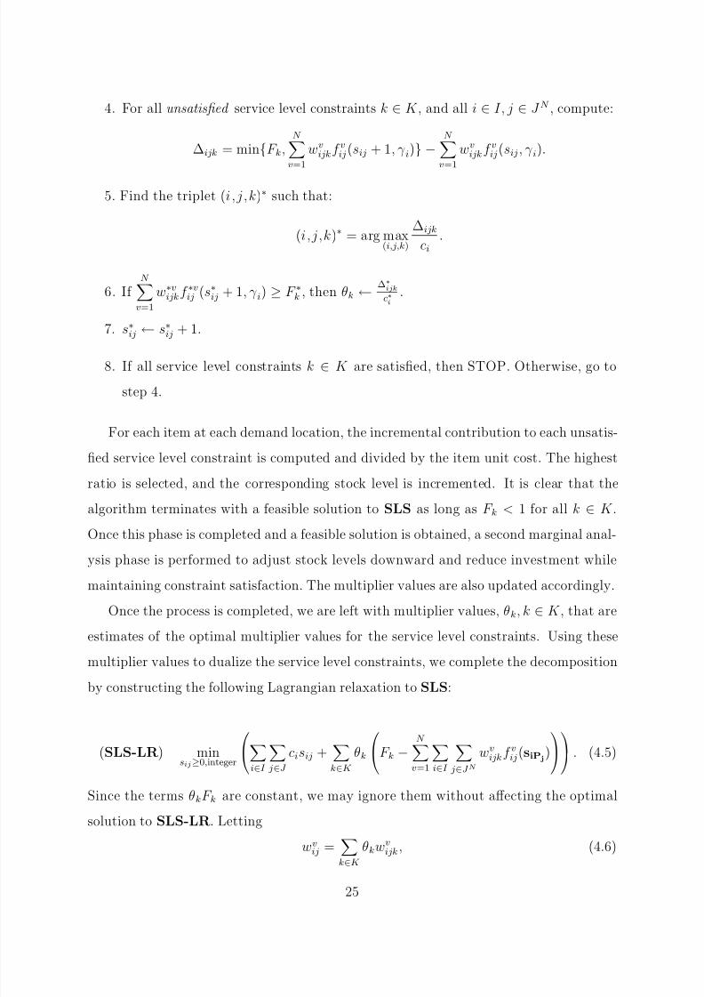
For each item at each demand location, the incremental contribution to each unsatis-
fied service level constraint is computed and divided by the item unit cost. The highest
ratio is selected, and the corresponding stock level is incremented. It is clear that the
algorithm terminates with a feasible solution to SLS as long as F k < 1 for all k ∈ K .
Once this phase is completed and a feasible solution is obtained, a second marginal anal-
ysis phase is performed to adjust stock levels downward and reduce investment while
maintaining constraint satisfaction. The multiplier values are also updated accordingly.
Once the process is completed, we are left with multiplier values, θk, k ∈ K , that are
estimates of the optimal multiplier values for the service level constraints. Using these
multiplier values to dualize the service level constraints, we complete the decomposition
by constructing the following Lagrangian relaxation to SLS:
(SLS-LR) minsij≥0,integer
i∈I
j∈J
cisij +k∈K
θk
F k −
N v=1
i∈I
j∈J N
wvijkf vij(siP j)
. (4.5)
Since the terms θkF k are constant, we may ignore them without affecting the optimal
solution to SLS-LR. Letting
wvij =
k∈K θkwvijk , (4.6)
25
8/3/2019 Industry Study on Parts Management and Ordering Strategy
http://slidepdf.com/reader/full/industry-study-on-parts-management-and-ordering-strategy 29/46
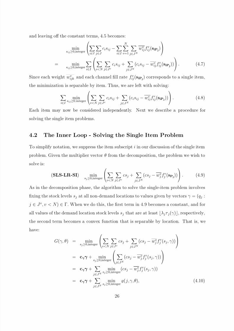
and leaving off the constant terms, 4.5 becomes:
minsij≥0,integer
i∈I
j∈J
cisij −i∈I
N v=1
j∈J N
wvijf vij(siP j)
= minsij≥0,integer
i∈I
v<N
j∈J v
cisij + j∈J N
(cisij − wvijf vij(siP j))
. (4.7)
Since each weight wvijk and each channel fill rate f vij(siP j) corresponds to a single item,
the minimization is separable by item. Thus, we are left with solving:
i∈I
minsij≥0,integer
v<N
j∈J v
cisij + j∈J N
(cisij − wvijf vij(siP j))
. (4.8)
Each item may now be considered independently. Next we describe a procedure for
solving the single item problems.
4.2 The Inner Loop - Solving the Single Item Problem
To simplify notation, we suppress the item subscript i in our discussion of the single item
problem. Given the multiplier vector θ from the decomposition, the problem we wish to
solve is:
(SLS-LR-SI) minsj≥0,integer
v<N
j∈J v
cs j + j∈J N
(cs j − wv j f v j (sP j)) . (4.9)
As in the decomposition phase, the algorithm to solve the single-item problem involves
fixing the stock levels s j at all non-demand locations to values given by vectors γ = (q j :
j ∈ J v, v < N ) ∈ Γ. When we do this, the first term in 4.9 becomes a constant, and for
all values of the demand location stock levels s j that are at least λ jτ j(γ ), respectively,
the second term becomes a convex function that is separable by location. That is, we
have:
G(γ, θ) = minsj≥0,integer
v<N
j∈J v
cs j + j∈J N
(cs j − wv j f v j (s j, γ ))
= cγ γ + minsj≥0,integer
j∈J N
(cs j − wv jf v j (s j , γ ))
= cγ γ + j∈J N
minsj≥0,integer
(cs j − wv jf v j (s j , γ ))
= cγ γ + j∈J N
minsj≥0,integer
g( j,γ,θ), (4.10)
26
8/3/2019 Industry Study on Parts Management and Ordering Strategy
http://slidepdf.com/reader/full/industry-study-on-parts-management-and-ordering-strategy 30/46
where cγ γ =v<N
j∈J v cq j and g( j,γ,θ) = (cs j − wv j f v j (s j, γ )) is discretely convex
in s j ≥ λ jτ j(γ ). Hence, by restricting our search to s j ≥ λ jτ j(γ ) for j ∈ J N ,
the stock levels minimizing g( j,γ,θ), j ∈ J N , can be found quickly and easily using
marginal analysis. That is, beginning with s j = λ jτ j(γ ), simply increase s j until
c > wv j
f v j (s j + 1, γ ) − f v j (s j, γ )
.
We now describe a rudimentary algorithm for solving SLS-LR-SI. Without loss of
generality, the location at the top level of the distribution network is assumed to be la-
beled location 1. Also, in what follows, the function nextS (·) accepts an integer argument
and returns the next highest value in the integer set S , or ∞ if the argument is greater
than or equal to the largest value in S (i.e., nextQ1(s1) returns min{q ∈ Q1 : q > s1} if
s1 < max{q : q ∈ Q1}; otherwise, ∞.)
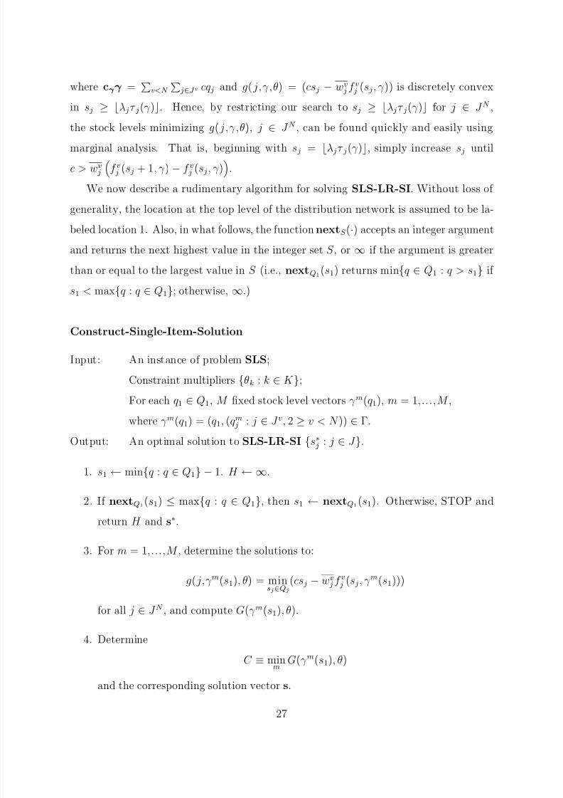
Construct-Single-Item-Solution
Input: An instance of problem SLS;
Constraint multipliers {θk : k ∈ K };
For each q1 ∈ Q1, M fixed stock level vectors γ m(q1), m = 1,...,M ,
where γ m(q1) = (q1, (qm j : j ∈ J v, 2 ≥ v < N )) ∈ Γ.
Output: An optimal solution to SLS-LR-SI {s∗ j : j ∈ J }.
1. s1 ← min{q : q ∈ Q1} − 1. H ← ∞.
2. If nextQ1(s1) ≤ max{q : q ∈ Q1}, then s1 ← nextQ1(s1). Otherwise, STOP and
return H and s∗.
3. For m = 1,...,M , determine the solutions to:
g( j,γ m(s1), θ) = minsj∈Qj
(cs j − wv jf v j (s j, γ m(s1)))
for all j ∈ J N , and compute G(γ m(s1), θ).
4. Determine
C ≡ minm
G(γ m(s1), θ)
and the corresponding solution vector s.
27
8/3/2019 Industry Study on Parts Management and Ordering Strategy
http://slidepdf.com/reader/full/industry-study-on-parts-management-and-ordering-strategy 31/46
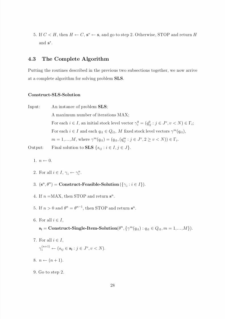
5. If C < H , then H ← C , s∗ ← s, and go to step 2. Otherwise, STOP and return H
and s∗.
4.3 The Complete Algorithm
Putting the routines described in the previous two subsections together, we now arrive
at a complete algorithm for solving problem SLS.
Construct-SLS-Solution
Input: An instance of problem SLS;
A maximum number of iterations MAX;
For each i ∈ I , an initial stock level vector γ 0i = (q0ij : j ∈ J v, v < N ) ∈ Γi;
For each i ∈ I and each qi1 ∈ Qi1, M fixed stock level vectors γ m(qi1),
m = 1,...,M , where γ m(qi1) = (qi1, (qmij : j ∈ J v, 2 ≥ v < N )) ∈ Γi.
Output: Final solution to SLS {sij : i ∈ I, j ∈ J }.
1. n ← 0.
2. For all i ∈ I , γ i ← γ ni .
3. (sn, θn) = Construct-Feasible-Solution ({γ i : i ∈ I }).
4. If n =MAX, then STOP and return sn.
5. If n > 0 and θn = θn−1, then STOP and return sn.
6. For all i ∈ I ,
si = Construct-Single-Item-Solution(θn, {γ m(qi1) : qi1 ∈ Qi1, m = 1,...,M }).
7. For all i ∈ I ,
γ (n+1)i ← (sij ∈ si : j ∈ J v, v < N ).
8. n ← (n + 1).
9. Go to step 2.
28

8/3/2019 Industry Study on Parts Management and Ordering Strategy
http://slidepdf.com/reader/full/industry-study-on-parts-management-and-ordering-strategy 32/46
Clearly the success of the algorithm described above hinges on the quality of the
γ i vectors that are chosen for each item i, as well as the number of vectors that are
examined. Since the number of items in large-scale problems can reach into the hundreds
of thousands, the number of vectors examined for each item must be small (i.e., less than
100). Based on our experience, we believe that for a given problem instance, it is possible
to describe characteristics that practical solution vectors are likely to have. In the next
section we provide an example problem that illustrates this point.
5 Example Problem
In this section we illustrate the concepts of this paper with an example problem. Figure 6
displays the structure of a three echelon distribution system with one level-1 location, two
level-2 locations and six level-3 locations. The transport lead time for all items at level-1
is 10 days; the lead time at level-2 is 5 days; and the lead time at level-3 is 2 days. For
each demand location, there are service level requirements of 90% instantaneous fill rate,
98% fill rate within two days, and 99.5% fill rate within seven days. These requirements
are based on the fill rates for all customer demands across all items at each location.
There are 18 service level constraints in all (three constraints for each of the six level-3
locations).
Figure 7 displays the daily demand rates for each item at each demand location. The
demand rates are relatively high for all items. The items are distinguished mainly by
their purchase cost, as Figure 8 reveals.
The optimization algorithm was used to find the stocking levels for the example
problem. In the resulting solution, all 18 service level constraints were binding. Figure 9displays the resulting stock levels, and Figure 10 displays these same stock levels expressed
as days of supply. To see the nature of the solution, the average location safety stock
level for each item (i.e., stock above the expected lead time demand), expressed in days
of supply, is displayed in Figure 11. There are many observations that can be made from
these results.
29

8/3/2019 Industry Study on Parts Management and Ordering Strategy
http://slidepdf.com/reader/full/industry-study-on-parts-management-and-ordering-strategy 33/46
Figure 6: Example Problem: Network Structure, Transit Times, and Service Level Con-
straints
Figure 7: Example Problem: Daily Demand Rates by Item and Demand Location
Figure 8: Example Problem: Item Purchase Cost
30
8/3/2019 Industry Study on Parts Management and Ordering Strategy
http://slidepdf.com/reader/full/industry-study-on-parts-management-and-ordering-strategy 34/46
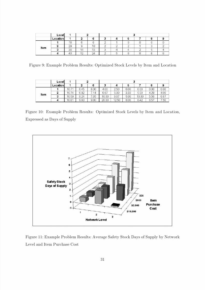
Figure 9: Example Problem Results: Optimized Stock Levels by Item and Location
Figure 10: Example Problem Results: Optimized Stock Levels by Item and Location,
Expressed as Days of Supply
Figure 11: Example Problem Results: Average Safety Stock Days of Supply by Network
Level and Item Purchase Cost
31
8/3/2019 Industry Study on Parts Management and Ordering Strategy
http://slidepdf.com/reader/full/industry-study-on-parts-management-and-ordering-strategy 35/46
First, relative to demand, the majority of the safety stock held in the system to
achieve the service level targets is held in the lower-cost, higher-demand rate items; that
is, items 3 and 4. It is also worth observing where the safety stock is held. The highest
cost item has essentially no safety stock at level-3, whereas the lower-cost, higher-demand
rate items have a considerable amount of safety stock at this level. The relative safety
stock levels for all but the lowest-demand, highest-cost item decrease for higher levels
in the network. The safety stock levels at level-1 are very low in all cases. The major
purpose of these upstream facilities is to keep the pipeline full, not to provide much in
the way of fill rate protection. Stocks at levels 2 and 3 provide that protection.
One of the reasons for using a multi-echelon model such as the one described in this
paper is to avoid making inappropriate inventory investments. For example, a single-
echelon model would tend at all levels to concentrate inventory in item 4 and have little
or no safety stock of item 1 at all levels. Observe that the optimal solution does not
have this characteristic at either level-1 or level-2. For example, at level-2, the relative
safety stock level for item 1 is higher than that for item 2. This allocation would not
have occurred if a single echelon model had been used to satisfy a level-2 fill rate target.
A similar observation holds, to a lesser extent, for items 2 and 3 at level 1.
Why did the model choose to invest so heavily in item 1 at level-2? Since there is
essentially no safety stock of item 1 at level-3, the instantaneous fill rate of this item
will be low. It would be even lower if the level-2 facility were frequently in a backorder
situation. To ensure the service level targets can be met, relatively more stock of item
1 is held at level-2. This increased stock permits a more predictable resupply time for
level-3 and prevents the instantaneous fill rate from degrading.
Another reason for using a multi-echelon model is that, without such a model, itwould be impossible to know what service level targets to establish for each item at each
of the levels to satisfy time-based service level constraints. The interaction of inventories
across levels and among items in determining service levels is extraordinarily complex.
No simple single-echelon model can accomplish this.
In section 4.1, we defined the set Γi to be the collection of all potential stock level
vectors for item i at levels v < N . The choice of vectors γ i ∈ Γi to be used in the
32

8/3/2019 Industry Study on Parts Management and Ordering Strategy
http://slidepdf.com/reader/full/industry-study-on-parts-management-and-ordering-strategy 36/46
optimization process should be based on the observations we have made from this example
problem. In particular, for low-cost, high-demand rate items, the vectors γ i should have
the following characteristics: level-2 stock levels will be high so that replenishment of
level-3 demand will occur quickly; thus the range of safety stock levels, measured in days
of supply would reflect this requirement. For high cost, low demand rate items, stock
levels at level 2 will be relatively moderate; on the other hand, level-1 stock levels, for all
items, will be relatively low. Thus, the number of vectors to be examined can be limited
in a practical manner so that the optimization problems are computationally tractable.
These observations apply to all of the situations we have encountered in practice.
The example demonstrates that the methodology does permit the optimization of
complex service level constraints in simple networks. Research is underway to apply the
approach to large scale problems.
6 An Initial Solution for Level-Specific Constraint
Sets
In this section we describe a linear programming approximation to SLS that produces
an initial vector for the overall algorithm that was described in Section 4. This approach
may be used for problem instances in which the service level constraints are level-specific;
that is, instances in which each service level constraint k is concerned with channel fill
rates at one and only one level v of the distribution network. Formally, the service level
constraints K are level-specific if K = ∪N v=1K v is a partitioning such that k ∈ K v only
if each corresponding weight wv
ijk = 0 for all v = v. (In practice, level-specific problem
instances are likely to be common.) We assume for the balance of this section that the
service level constraints of our problem instance are level-specific.
Our approach is to reformulate SLS in terms of echelon stock variables and to ap-
proximate the fill rate expressions in the service level constraints using these variables. In
our approximation scheme, each fill rate expression can be expressed in terms of a single
echelon stock variable, rather than the vector of channel stock levels as in the original
33

8/3/2019 Industry Study on Parts Management and Ordering Strategy
http://slidepdf.com/reader/full/industry-study-on-parts-management-and-ordering-strategy 37/46
formulation. Furthermore, all of the constraints for levels 1, 2,...,N − 1 are replaced
by aggregate constraints: one for each location in the level. The resulting problem is a
mixed-integer linear program whose linear relaxation yields a solution that can be used
to initialize the SLS algorithm. The solution to the linear program can be improved by
adjusting the probabilities to reflect higher echelon shortages and then re-solving. This
adjustment step can be repeated a small number of times.
For level-specific service level constraints, the problem SLS can be written as:
minimize
i∈I j∈J cisij
subject toi∈I
j∈J N
wvijkf vij
siP j
≥ F k, ∀k ∈ K v, v = 1, 2..., N,
sij ≥ λijT ij and integer, ∀i ∈ I, j ∈ J.
Recall from Section 4 that in the overall solution algorithm we are interested in findingθk : k ∈ ∪N v=1K v
, the multiplier values (i.e., dual variables) associated with the service
level constraints in this problem. The method we describe in this section will result in
approximations for these multiplier values.
Let S j denote the set of of all locations at or below location j in the network hierarchy.
Let xij denote the echelon stock of item i beginning at location j :
xij = j∈S j
sij .
Let s( j) denote the set of immediate successors to location j and interpret s( j) = ∅ for
j ∈ J N
. Inverting the relationship, we have:
sij = xij − j∈s( j)
xij
for all i ∈ I, and j ∈ J (a null sum on the right hand side is taken to be zero). The
objective of SLS can be re-expressed as:
minimizei∈I
j∈J 1
cixij.
34

8/3/2019 Industry Study on Parts Management and Ordering Strategy
http://slidepdf.com/reader/full/industry-study-on-parts-management-and-ordering-strategy 38/46
Let X ij denote the random variable that measures the number of demands for product
i at location j occurring over a replenishment lead time for item i from location p( j).
(For calculation purposes, we assume that X ij has a negative binomial distribution with
known mean and variance. Initially, we assume it has a Poisson distribution with mean
λijT ij. In subsequent iterations, we capture the impacts of shortages at location p( j) and
adjust the mean and variance of X ij accordingly.)
We assume that for a given item i and a given location j at level v, all locations
at level N which are below j will experience the identical probability of filling orders
within the transport lead time from location j . Letting v( j) denote the level of j, we
approximate this probability with the probability that stock exists at some location in
S j to satisfy the demand:
f v( j)ij
siP j
≈ Pr[X ij ≤ xij]
for all j ∈ S j∩J N . This rough approximation is employed to find a good starting solution
to SLS quickly. More accurate service level calculations are employed later to refine this
solution.
Recalling that P j(v) denotes the unique ancestor of location j ∈ J N at level v, the
service level constraints can be approximated using:i∈I
j∈J N
wvijk Pr[X iP j(v) ≤ xiP j(v)] ≥ F k, ∀k ∈ K v, v = 1,...,N.
Reordering terms in the summation, these become:
i∈I
j∈J v
j∈J N ∩S ( j)
wvijk
Pr[X ij ≤ xij] ≥ F k, ∀k ∈ K v, v = 1,...,N.
Extending the previous definition of wijk to all locations j (not just j ∈ J N ), we let
wijk = j∈J N ∩S ( j) wvijk for all j ∈ J . Thus, for non-demand locations j, wijk denotes the
fraction of demand associated with service level constraint k that is for part i at any of
the demand locations j ∈ J N ∩ S j . That is, wijk is the probability that a demand under
contract k is for part i at some location in J N ∩ S ( j). The approximating constraints
now become:
i∈I j∈J vwijk Pr[X ij ≤ xij] ≥ F k, ∀k ∈ K v, v = 1,...,N.
35
8/3/2019 Industry Study on Parts Management and Ordering Strategy
http://slidepdf.com/reader/full/industry-study-on-parts-management-and-ordering-strategy 39/46
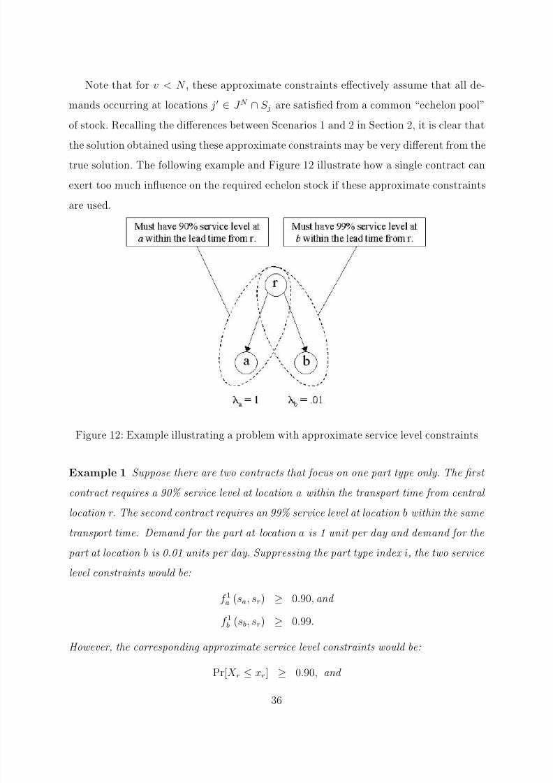
Note that for v < N , these approximate constraints effectively assume that all de-
mands occurring at locations j ∈ J N ∩ S j are satisfied from a common “echelon pool”
of stock. Recalling the differences between Scenarios 1 and 2 in Section 2, it is clear that
the solution obtained using these approximate constraints may be very different from the
true solution. The following example and Figure 12 illustrate how a single contract can
exert too much influence on the required echelon stock if these approximate constraints
are used.
Figure 12: Example illustrating a problem with approximate service level constraints
Example 1 Suppose there are two contracts that focus on one part type only. The first
contract requires a 90% service level at location a within the transport time from central
location r. The second contract requires an 99% service level at location b within the same
transport time. Demand for the part at location a is 1 unit per day and demand for the
part at location b is 0.01 units per day. Suppressing the part type index i, the two service
level constraints would be:
f 1a (sa, sr) ≥ 0.90, and
f 1b (sb, sr) ≥ 0.99.
However, the corresponding approximate service level constraints would be:
Pr[X r ≤ xr] ≥ 0.90, and
36

8/3/2019 Industry Study on Parts Management and Ordering Strategy
http://slidepdf.com/reader/full/industry-study-on-parts-management-and-ordering-strategy 40/46
Pr[X r ≤ xr] ≥ 0.99.
Obviously, the second of these two constraints will dominate the solution, even though it
is associated with only a small fraction of the demand. Thus, the solution will place a larger amount of stock than is needed within the subtree, because the magnitude of location
a’s demand relative to the overall demand placed on location r is ignored, and there is no
notion that the stock xa placed at location a is dedicated to servicing location a.
The difficulty described above arises with constraints at levels v = 1, 2,...,N − 1. To
overcome it, we construct another set of non-negative weights, {ωlk ≥ 0 : l ∈ J v, k ∈ K v,
v ∈ {1, 2,...,N − 1}} with the property that
k∈K v
ωlk = 1, ∀l ∈ J v, v ∈ {1, 2,...,N − 1}.
Specifically, if each contract k ∈ K v corresponds to a different customer and if λijk
denotes the demand rate for part i at location j ∈ J N for the customer corresponding to
contract k, then we use the following weights:
ωlk = i∈I
j∈J N ∩S (l) λijk
k∈K v
i∈I j∈J N ∩S (l) λijk
, ∀l ∈ J v, k ∈ K v, v ∈ {1, 2,...,N − 1}.
When the demand processes are Poisson, the weight ωlk describes the probability that a
demand occurring in the network below location l is from the customer associated with
contract k.
For each v ∈ {1, 2,...,N − 1}, given the weights {ωlk; l ∈ J v, k ∈ K v}, we replace the
service level constraints in K v with a set of aggregate constraints, where each location
l ∈ J v is represented by a single constraint:
k∈K v
ωlki∈I
j∈J v
wijk Pr[X ij ≤ xij] ≥k∈K v
ωlkF k
Intuitively, we associate with each echelon location l ∈ J v a service level constraint that is
a weighted average over all contracts at that level, where the weights capture the relative
importance of each contract within that echelon. Note that locations other than l may
contribute to the constraint associated with l; i.e., there may exist wijk > 0 for some i
and some j = l.
37

8/3/2019 Industry Study on Parts Management and Ordering Strategy
http://slidepdf.com/reader/full/industry-study-on-parts-management-and-ordering-strategy 41/46
For each level v ∈ {1, 2,...,N }, let Lv denote the set that indexes the constraints at
level v, so that:
L
v
=
J v, v ∈ {1, 2,...,N − 1};
K N , v = N.
Then, for each i ∈ I, l ∈ Lv, j ∈ J v(l), let
uijl =
k∈K v ωlkwijk , l ∈ Lv, v ∈ {1, 2,...,N − 1};
wN ijl , l ∈ LN .
Finally, let
F l =
k∈K v ωlkF k, l ∈ Lv, v ∈ {1, 2,...,N − 1};
F l, l ∈ LN
.The approximation to SLS can now be written as:
(Approx-SLS) minimizei∈I
j∈J 1
cixij
subject toi∈I
j∈J
uijl Pr[X ij ≤ xij] ≥ F l , ∀l ∈ Lv, v = 1, 2,...,N,
xij − j
∈s( j)
xij ≥ λijT ij and integer, ∀i ∈ I, j ∈ J.
Let
ϕl : l ∈ ∪N v=1Lv
denote the multipliers to the service level constraints in this prob-
lem. Using this dual solution to Approx-SLS, we can construct an approximate dual
solution for SLS. Comparing SLS with Approx-SLS, we want the dual solutions of the
two problems to satisfy:N v=1
l∈Lv
ϕlF l =N v=1
k∈K v
θkF k.
A simple way to achieve this is to set:
θk =
l∈Lv ωlkϕl k ∈ K v, v < N,
ϕk k ∈ K N .
Thus, a dual solution to Approx-SLS can give rise to dual variables on the service level
constraints in SLS.
Approx-SLS is amenable to linear programming approximations. Let Γ represent a
set of pre-determined values for echelon stock, and let Γ ij ⊆ Γ be a finite subset of those
38
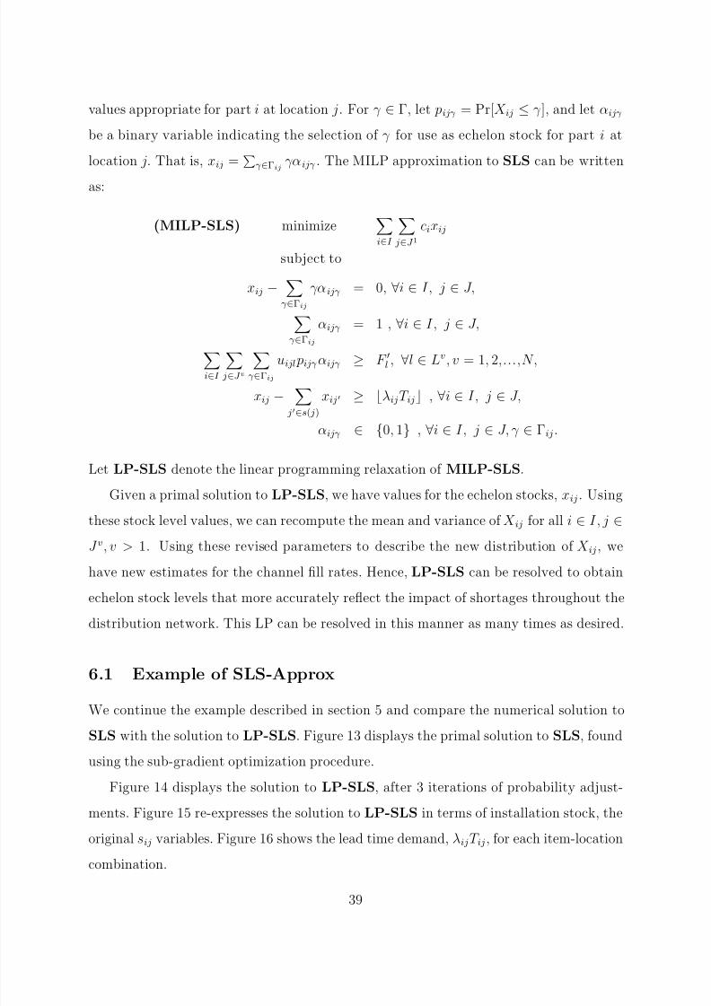
8/3/2019 Industry Study on Parts Management and Ordering Strategy
http://slidepdf.com/reader/full/industry-study-on-parts-management-and-ordering-strategy 42/46
values appropriate for part i at location j. For γ ∈ Γ, let pijγ = Pr[X ij ≤ γ ], and let αijγ
be a binary variable indicating the selection of γ for use as echelon stock for part i at
location j. That is, xij = γ ∈Γij γαijγ . The MILP approximation to SLS can be written
as:
(MILP-SLS) minimizei∈I
j∈J 1
cixij
subject to
xij −γ ∈Γij
γαijγ = 0, ∀i ∈ I, j ∈ J,
γ ∈Γij
αijγ = 1 , ∀i ∈ I, j ∈ J,
i∈I
j∈J v
γ ∈Γij
uijl pijγ αijγ ≥ F l , ∀l ∈ Lv, v = 1, 2,...,N,
xij − j∈s( j)
xij ≥ λijT ij , ∀i ∈ I, j ∈ J,
αijγ ∈ {0, 1} , ∀i ∈ I, j ∈ J, γ ∈ Γij.
Let LP-SLS denote the linear programming relaxation of MILP-SLS.
Given a primal solution to LP-SLS, we have values for the echelon stocks, xij . Using
these stock level values, we can recompute the mean and variance of X ij
for all i ∈ I, j ∈
J v, v > 1. Using these revised parameters to describe the new distribution of X ij, we
have new estimates for the channel fill rates. Hence, LP-SLS can be resolved to obtain
echelon stock levels that more accurately reflect the impact of shortages throughout the
distribution network. This LP can be resolved in this manner as many times as desired.
6.1 Example of SLS-Approx
We continue the example described in section 5 and compare the numerical solution to
SLS with the solution to LP-SLS. Figure 13 displays the primal solution to SLS, found
using the sub-gradient optimization procedure.
Figure 14 displays the solution to LP-SLS, after 3 iterations of probability adjust-
ments. Figure 15 re-expresses the solution to LP-SLS in terms of installation stock, the
original sij variables. Figure 16 shows the lead time demand, λijT ij, for each item-location
combination.
39

8/3/2019 Industry Study on Parts Management and Ordering Strategy
http://slidepdf.com/reader/full/industry-study-on-parts-management-and-ordering-strategy 43/46
Figure 13: Echelon stock solution to SLS
Figure 14: Echelon stock solution to LP-SLS
Figure 15: Installation stock solution to LP-SLS
Figure 16: Lead Time Demand
40

8/3/2019 Industry Study on Parts Management and Ordering Strategy
http://slidepdf.com/reader/full/industry-study-on-parts-management-and-ordering-strategy 44/46
Observe, by comparing Figures 13 and 14, that the solution to LP-SLS understates
the amount of stock that is required to achieve the target service level constraints for
the upper two levels (levels 1 and 2). This is not surprising because the approximation
assumes that stock at lower levels can be shared within each echelon to satisfy demands
that arise. Less inventory would be needed if such sharing could indeed take place. In the
case of locations 1 and 6, setting installation stock (Figure 15) equal to the floor of lead
time demand (Figure 16) for all items is sufficient to satisfy the aggregate approximate
fill rate constraints. On the other hand, the solution to LP-SLS is quickly obtained and
exhibits similar characteristics to the SLS solution (concentration of inventory in lower
demand rate items).
7 Conclusions
In this paper we described a continuous review inventory model for a multi-item, multi-
echelon distribution system for service parts in which complex service level constraints
exist for general groups of items across multiple locations and distribution channels.
First, we derived exact fill rate expressions for each item’s distribution channel. Next,
we developed a solution approach for determining target inventory levels that meet all
service level constraints at minimum investment. Finally, we described how a linear
programming model could be used to seed the solution approach for special types of
problem instances.
References
Agrawal, N. and Cohen, M. A. (2001), “Optimal Material Control in an Assembly System
with Component Commonality,” Naval Research Logistics, 48, 409–429.
Cheung, K. L. and Hausman, W. H. (1995), “Multiple Failures in a Multi-Item Spares
Inventory Model,” IIE Transactions, 27, 171–180.
41

8/3/2019 Industry Study on Parts Management and Ordering Strategy
http://slidepdf.com/reader/full/industry-study-on-parts-management-and-ordering-strategy 45/46
Cohen, M., Kleindorfer, P., and Lee, H. L. (1986), “Optimal Stocking Policies for Low
Usage Items in Multi-Echelon Inventory Systems,” Naval Research Logistics Quarterly ,
33, 17–38.
— (1989), “Near-Optimal Service Constrained Stocking Policies for Spare Parts,” Oper-
ations Research , 37, 104–117.
Cohen, M. and Lee, H. L. (1988), “Strategic Analysis of Integrated Production-
Distribution Systems: Models and Methods,” Operations Research , 36, 216–228.
Feeney, G. J. and Sherbrooke, C. C. (1966), “The (S-1,S) Inventory Policy under Com-
pound Poisson Demand,” Management Science, 12, 391–411.
Graves, S. (1982), “A Multiple-Item Inventory Model with a Job Completion Criterion,”
Management Science, 28, 1334–1337.
Graves, S. C. (1985), “A Multi-Echelon Inventory Model for a Repairable Item with
One-for-One Replenishment,” Management Science, 31, 1247–1256.
Hausman, W. H., Lee, H. L., and Zhang, A. X. (1998), “Joint Demand Fulfillment
Probability in a Multi-Item Inventory System with Independent Order-Up-To Policies,”
European Journal of Operational Research , 109, 646–659.
Mamer, J. W. and Smith, S. A. (1982), “Optimizing Field Repair Kits Based on Job
Completion Rate,” Management Science, 28, 1328–1333.
Muckstadt, J. A. (1973), “A Model for a Multi-Item, Multi-Echelon, Multi-Indenture
Inventory System,” Management Science, 20, 472–481.
Pyke, D. F. (1990), “Priority Repair and Dispatch Policies for Repairable-Item Logisitics
Systems,” Naval Research Logistics, 37, 1–30.
Rustenburg, W. D., van Houtum, G. J., and Zijm, W. H. M. (2001), “Spare Parts
Management at Complex Technology-Based Organizations: An Agenda for Research,”
International Journal of Production Economics, 71, 177–193.
42
8/3/2019 Industry Study on Parts Management and Ordering Strategy
http://slidepdf.com/reader/full/industry-study-on-parts-management-and-ordering-strategy 46/46
Schmidt, C. P. and Nahmias, S. (1985), “Optimal Policy for a Two-Stage Assembly
System Under Random Demand,” Operations Research , 33, 1130–1145.
Sherbrooke, C. C. (1968), “METRIC: A Multi-Echelon Technique for Recoverable ItemControl,” Operations Research , 16, 122–141.
— (1971), “An Evaluator for the Number of Operationally Ready Aircraft in a Multi-Item
Supply System,” Operations Research , 19, 618–635.
— (1986), “VARI-METRIC: Improved Approximations for Multi-Indenture, Multi-
Echelon Availability Models,” Operations Research , 34, 311–319.
Silver, E. A. (1972), “Inventory Allocation Among and Assembly and its Repairable
Subassemblies,” Naval Research Logistics Quarterly , 19, 261–280.
Smith, S. A., Chambers, J. C., and Shlifer, E. (1980), “Optimal Inventories Based on
Job Completion Rate for Repairs Requiring Multiple Items,” Management Science, 26,
849–852.
Song, J.-S. (1998), “On the Order Fill Rate in a Multi-Item, Base-Stock Inventory Sys-
tems,” Operations Research , 46, 831–845.
Song, J.-S., Xu, S. H., and Liu, B. (1999), “Order-Fulfillment Performance Measures in
an Assemble-To-Order System with Stochastic Leadtimes,” Operations Research , 47,
131–149.
Svoronos, A. and Zipkin, P. (1991), “Evalutation of One-for-One Replenishment Policies
for Multiechelon Inventory Systems,” Management Science, 37, 68–83.
Yano, C. A. (1987), “Stochastic Leadtimes in Two-Level Assembly Systems,” IIE Trans-
actions, 19, 371–378.