Industry Momentum and Behavioral Limits to Arbitrage

Lukas Menkhoff, University of Hannover, Germany and

Maik Schmeling, University of Hannover, Germany JEL-Classification: G 23, G 14 Keywords: momentum trading, market efficiency, prospect theory April 28, 2004 We would like to thank Ulrich Berz, Stephen Schneider, Martin Weber and in particular Carol Osler for very useful comments and Markus Glaser and Martin Weber for sharing data with us. Corresponding: Lukas Menkhoff, Department of Economics, University of Hannover, Königsworther Platz 1, D-30167 Hannover, Germany, menkhoff@gif.uni-hannover.de

Industry Momentum and Behavioral Limits to Arbitrage

Abstract: Momentum trading based on German industries robustly generates significant profits that cannot be explained by risk-based approaches. Industry momentum is positively related to individual stock momentum. Its return pattern is consistent with under- and overreaction. We propose a behavioral explanation as to why momentum profits may not be easily arbitraged away: the prospective utility of momentum strategies only becomes superior to buy & hold for horizons of 6 to 12 months and longer. The most relevant institutional investors, however, appear to be more short-term oriented. Modifications of momentum trading in order to increase utility show a strong return-utility trade-off.

2

Industry Momentum and Behavioral Limits to Arbitrage

1 Introduction

The ongoing observation of momentum in stock markets is encouraging a

growing amount of research. Momentum investing means to buy past winners and to

sell past losers. Evidence shows that this simple trading rule generates profits in the

order of 10 per cent p.a. that cannot yet be fully explained by risk-based or other

approaches. We contribute to this puzzle by examining the less researched industry

momentum for Germany. The findings echo stylized facts from earlier studies, but

also reveal an unusually long 30 month period of increasing cumulative momentum

returns. This particularly strong momentum phenomenon is a challenge to market

efficiency. We propose a behavioral explanation – based on prospect theory – as to

why momentum may not be easily arbitraged away.

Empirical studies have so far mostly focused on individual stock momentum.

Following the seminal paper of Jegadeesh and Titman (1993) for the US,

Rouwenhorst (1998) proved the existence of momentum profits for European

markets. Momentum profits also exist, but to a lower degree in emerging markets

(Rouwenhorst, 1999). Due to the worldwide coverage, data mining may not be a

convincing explanation. Robustness is highlighted by Jegadeesh and Titman (2001),

who showed the continuing profitability of momentum investing in an out-of-sample

period for the US. Finally, Griffin, Ji and Martin (2003) examine all available markets

in the world and strengthen the momentum puzzle.

Efforts to explain momentum return by high risks taken include unsuccessful

relations to market risk (Jegadeesh and Titman, 1993), the unconditional three-factor

model of Fama and French (1996), and its conditional application by Grundy and

Martin (2001). More recently, macro factors have been investigated: Chordia and

Shivakumar (2002) find strong explanatory power of macro risk for momentum

returns in the US, but Cooper, Gutierrez and Hameed (2003) question the robustness

of that finding and propose a relation to market states, i.e. up and down markets.

Griffin, Ji and Martin (2003) conclude that both relations – to macro factors and to

market states – are an exception specific to the US when compared with evidence

from 39 other stock markets in the world.

3

It may thus be no surprise that behavioral approaches for explaining momentum

returns are often regarded as most convincing. Jegadeesh and Titman (1993)

already proposed "underreaction" to new information as a plausible explanation.

Models by Barberis, Shleifer and Vishny (1998), Daniel, Hirshleifer and

Subrahmanyam (1998) and Hong and Stein (1999) formalize how an established

behavioral pattern might cause under- and overreaction in asset prices. Jegadeesh

and Titman (2001) demonstrate that cumulative momentum returns show a

corresponding pattern over time: they first increase – reflecting the overreaction –

and then they decrease – reflecting the return to more fundamental valuation – so

that marginal returns become negative. This pattern over time is a key element in

favor of the behavioral approaches. It has been reproduced in other studies too; see

e.g. Griffin, Ji and Martin (2003). More recent work uses the established finding of

asymmetries in risk perception as a building block to explain momentum returns

(Ang, Chen and Xing, 2001; Grinblatt and Han, 2002).

We apply risk-based and behavioral explanations as they have been used in the

above described studies to industry momentum. It seems justified to transfer

analytical approaches from the individual to the industry level, following the early

study of Moskowitz and Grinblatt (1999). They have claimed that industry momentum

would dominate individual stock momentum. Grundy and Martin (2001) and Chordia

and Shivakumar (2002) show that both forms of momentum coexist in the US stock

market.

We use data based on the broad German CDAX index for the years 1973 to

2002. The index covered about 750 stocks at the end of 2002, i.e. almost all German

stocks being traded at the Frankfurt stock exchange. As we are interested in industry

momentum, the analysis relies on the usual classification into 19 industries.

We find that in Germany, industry momentum indeed exists and generates

excess returns comparable in size to individual stock momentum. Moreover, trading

rules based on industry and individual stock momentum are positively correlated but

clearly different. In accordance with Moskowitz and Grinblatt (1999), there is also no

January effect in the German industry data. The German data differ from the US

data, however, in that industry momentum prevails not only up to a 12-month holding

period, but up to 30 months. The pattern of cumulative momentum returns shows a

clear hump-shaped pattern with increasing holding periods and thus accords well

with an underreaction-overreaction explanation.

4

Building on the influence of asymmetric risk perception, we propose a

behavioral explanation for the observable non-arbitrage. Cumulative prospect theory,

when applied with established empirical parameters to the risk-return profiles of the

buy & hold strategy and momentum strategies, reveals the importance of horizon

(see Benartzi and Thaler, 1995). Momentum strategies yield a lower "prospective

utility" up to 6 to 12-month horizons and longer, which is beyond the relevant

investment horizon of most institutional investors. If the prospect theory – and the

usual coefficients found – correctly describe the behavior and utility of stock

investors, they face a problem that has first been analyzed for stock investment by

Benartzi and Thaler (1995): short-term return characteristics makes the long-term

superior strategy unattractive in utility terms. Whereas Benartzi and Thaler (1995)

want to explain the risk premium of stock holdings in general, we are concerned with

the risk premium – in the sense described – of momentum trading.

As possible reaction to lower the high momentum trading risk – as identified by

prospect theory – investors may modify the benchmark momentum strategy in two

ways: increasing portfolio size and formation/holding period. In a systematic analysis

of these determinants of prospective utility we find that both parameters have a

critical impact on prospective utilities but also on return distributions. Varying these

parameters in a simplified regression framework yields a clear utility-return trade-off

for momentum investors: higher returns due to following momentum strategies lead

to lower utility.

Consequently, we find that institutional investors may not have an incentive to

apply an industry momentum strategy in Germany within an investment time frame of

six months or even longer. Possible attempts to increase utility by choosing less risky

momentum strategies tend to fail: expected prospective utility of momentum trading

equals the one of the market portfolio only when the market portfolio is held. Thus,

the application of prospect theory claims that a respective valuation of momentum

returns can largely wipe out excess returns and thereby confirms "behaviorally

adjusted" efficient markets.

The paper is structured into three more sections. Section 2 shows the existence

and characteristics of the industry momentum in Germany. Section 3 contains the

findings of the behavioral approach. Section 4 concludes.

2 Industry momentum in Germany

5

2.1 Data The universe of stocks we are examining is defined by the CDAX. The market

capitalization of the CDAX makes up for almost all German stocks being traded at

the Frankfurt Stock exchange and is thus a quite representative measuring stick of

the German stock market. It is the broadest available measure of stocks being traded

in the German market. At the end of 2002 it comprised of approximately 750 stocks,

among them the more well known 30 stocks of the German DAX index as well as the

new technology stocks being traded in the Tec-DAX segment.

The CDAX is divided into 19 industries, of which 17 are available for the whole

30-year period of examination from 1.1.1973 to 1.1.2003. The index for the software

industry is available only for about 14 years and the index for media for about 17

years. Moreover, the Deutsche Boerse AG provides the now valid industry indices

only starting in 1987. For the earlier years, we rely on backwards calculation by

Thomson Financial Datastream, which is the most established source for this

purpose.

A description of the 19 industries, including their average share of market

capitalization and further valuation indicators can be found in Table 1. We slightly

adjust the standard Jegadeesh and Titman (1993, 2001) momentum calculation

approach. We analyze monthly returns relative to the market return to match the

benchmark orientation of investment managers. By comparison, Moskowitz and

Grinblatt (1999) use monthly returns in excess of the risk-free rate, adjusted for size

and book-to-market effects. We cannot reproduce this latter approach as book values

are not available for industries. However, size and valuation do not seem to explain

momentum returns in the US.1 Table 1 reveals that the German industries' excess

returns, with the one exception of the software industry, are not significantly different

from zero.

2.2 Momentum returns To create portfolios we follow Jegadeesh and Titman (2001). Stocks are divided

into 19 industries. The industry indices are then ordered by their most recent returns.

Thereafter, two decisions have to be made: first, how many indices are held in the

1 Calculations presented in Section 2.4 below indicate – in agreement with the literature – that neither size nor common valuation ratios help to explain German industry momentum returns.

6

winner and loser portfolios each (parameter "n"). Second, how long are the formation

("f") and holding period ("h")? Jegadeesh and Titman (2001) symmetrically choose

the extreme decile portfolios and prefer a six-month strategy. Their n-f-h design can

thus be described as 1-6-6. For comparison, Moskowitz and Grinblatt (1999) choose

the three best and worst industries (out of a total of 20). Regarding the formation

period, they present figures between one and twelve months; regarding the holding

period, they give results between 1 and 36 months.

In this paper we regard the 1-6-6 strategy as the benchmark configuration, and

consider further configurations for robustness purposes. In accordance with the

literature, the winner and loser portfolios are of the same amount so that the trading

strategy is largely self-financing. The stocks are weighted by their capitalization

within the industries, but industries are weighted equally in the case of portfolios with

n>1 industries.

Table 2 presents the main findings for the strategy 1-6-h, distinguishing

contributions from winner, medium and loser portfolios. For brevity, only the average

monthly raw returns for the best, medium and worst portfolios are shown over several

holding periods h between 6 and 60 months. In addition, returns for long-short

strategies are documented, starting with the difference between the winner and loser

portfolios. This difference is then split up in two contributions that are divided by the

medium portfolio return. One can see that the buy side clearly dominates the sell

side, as it is larger in all cases shown. This is in agreement with the finding of

Moskowitz and Grinblatt (1999, p. 1272). On average, the buy side makes up for over

70% of the momentum profits in the 1-6-h strategy.2

We next evaluate whether these strategies still look profitable after adjustment

for transaction costs. In this respect we assume that the rebalancing takes place

every six months only. By contrast, monthly adjustment would cause the running of

overlapping portfolios. The lower frequency of adjustment avoids distorted t-statistics

for the benchmark strategy. Half-yearly rebalancing as applied here is a conservative

procedure in that overlapping portfolios may generate higher momentum returns.

However, procedure does not dominate findings: the 1-6 benchmark strategy, for

example, generates a monthly momentum return of 1.10% for overlapping portfolios

compared to 1.05% for the more cautious procedure. Not surprisingly, the correlation

2 We will consider only symmetric strategies with f=h for the rest of the paper, so we can suppress the second parameter when referring to a strategy: e.g. 1-6-6 becomes 1-6.

7

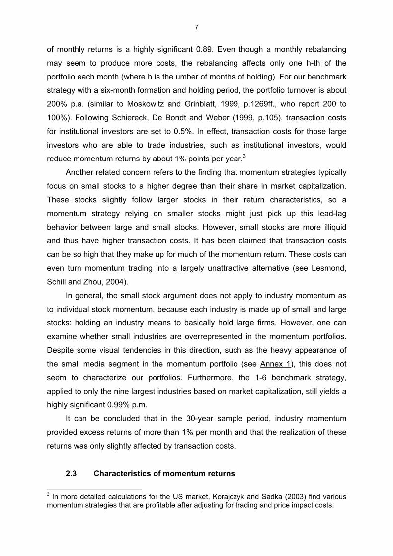
of monthly returns is a highly significant 0.89. Even though a monthly rebalancing

may seem to produce more costs, the rebalancing affects only one h-th of the

portfolio each month (where h is the umber of months of holding). For our benchmark

strategy with a six-month formation and holding period, the portfolio turnover is about

200% p.a. (similar to Moskowitz and Grinblatt, 1999, p.1269ff., who report 200 to

100%). Following Schiereck, De Bondt and Weber (1999, p.105), transaction costs

for institutional investors are set to 0.5%. In effect, transaction costs for those large

investors who are able to trade industries, such as institutional investors, would

reduce momentum returns by about 1% points per year.3

Another related concern refers to the finding that momentum strategies typically

focus on small stocks to a higher degree than their share in market capitalization.

These stocks slightly follow larger stocks in their return characteristics, so a

momentum strategy relying on smaller stocks might just pick up this lead-lag

behavior between large and small stocks. However, small stocks are more illiquid

and thus have higher transaction costs. It has been claimed that transaction costs

can be so high that they make up for much of the momentum return. These costs can

even turn momentum trading into a largely unattractive alternative (see Lesmond,

Schill and Zhou, 2004).

In general, the small stock argument does not apply to industry momentum as

to individual stock momentum, because each industry is made up of small and large

stocks: holding an industry means to basically hold large firms. However, one can

examine whether small industries are overrepresented in the momentum portfolios.

Despite some visual tendencies in this direction, such as the heavy appearance of

the small media segment in the momentum portfolio (see Annex 1), this does not

seem to characterize our portfolios. Furthermore, the 1-6 benchmark strategy,

applied to only the nine largest industries based on market capitalization, still yields a

highly significant 0.99% p.m.

It can be concluded that in the 30-year sample period, industry momentum

provided excess returns of more than 1% per month and that the realization of these

returns was only slightly affected by transaction costs.

2.3 Characteristics of momentum returns

3 In more detailed calculations for the US market, Korajczyk and Sadka (2003) find various momentum strategies that are profitable after adjusting for trading and price impact costs.

8

This section further elaborates on characteristics of the 1-6 momentum strategy.

It has been found that industry and individual stock momentum are positively related

(Moskowitz and Grinblatt, 1999), but that they are not the same (Grundy and Martin,

2001, Chordia and Shivakumar, 2002). We cannot rigorously test this relationship

with our industry data as they do not provide information on individual stock returns.

However, the German data from Glaser and Weber (2003) for individual stock

momentum of 446 titles in the period 6/1988 to 7/2001 can be largely compared with

our industry momentum return over the same period. Consistent with the literature,

there is positive, significant correlation of 0.34.

Moreover, as shown in virtually any other study on momentum trading, the

CAPM beta measure of risk cannot explain momentum returns (see e.g. Grundy and

Martin, 2001). In the German industry momentum case, the beta coefficients are

below rather than above unity, even though momentum trading generates

remarkable returns beyond the market return (see Table 3).

Another aspect of momentum trading that has been studied in detail is the

pronounced January effect. The Jegadeesh and Titman (1993) study had already

documented that winner portfolios outperform loser portfolios in all months except

January. This finding has been repeated, for example in Jegadeesh and Titman

(2001) and in other individual stock momentum studies, but has been neglected in

the US industry momentum analysis of Moskowitz and Grinblatt (1999). This

discrepancy does not seem to be surprising, as the standard understanding of a

January effect refers to tax-motivated trading, i.e. to sell stocks in December in order

to gain from realized losses and buy back stocks in January (see Grinblatt and

Moskowitz, 2003). This effect refers to certain individual stocks which will not

exclusively be represented in an industry. So, a loser industry will probably contain

some losing firms but the relation between losing industries and losing firms is not

necessarily tight which will dilute the January effect on the industry aggregation level.

For the German 1-6-6 industry momentum, we even find that losers tend to lose

further in January, enhancing profits on the momentum portfolio rather than

eviscerating them (see Table 4).

As a final characteristic that has received much attention, it seems worthwhile to

examine underreaction and overreaction, a phenomenon documented by Jegadeesh

and Titman (2001). Figure 1 shows that for the 1-6 and 1-12 strategies, the pattern of

winner, loser and momentum returns for a period of up to 60 months after portfolio

9

formation. Several facts stand out from this graph: First, momentum profits continue

for up to 30 months. Second, cumulative returns stagnate or even begin to decrease

after 30 months. Finally, the pattern described above is quite stable for other

strategies and the sub-samples 1973-1987 and 1988-2002 (see Annex 2).

The pattern of excess momentum return for German industries is thus

consistent with the literature – with one considerable exception: the phase of

increasing profits is markedly longer than typically found for individual momentum

strategies. Note, however, that regarding industry momentum in the US, Moskowitz

and Grinblatt (1999, p.1273) report persistence of sell-side profits for 24 or even 36

months. It may be reassuring in this respect that individual momentum strategies for

the US and Germany share many parallels (Schiereck, De Bondt and Weber, 1999)

but that Glaser and Weber (2003) also report persistence in German individual stock

momentum returns beyond a 12 months holding period. One interpretation might

focus on information processing: if one sees increasing momentum returns as an

indication of time-consuming information processing, this would suggest that the

German market is possibly less efficient than the US market.4

In summary, the characteristics of industry momentum in German stocks fit by

and large into the literature, even though the long under- and overreaction period

may have been unexpected ex ante.

2.4 Robustness of momentum returns In a final step to establish the existence of industry momentum in Germany,

some robustness checks are performed. We first alter the configuration of the

standard 1-6 momentum strategy. From the universe of possible modifications that

can be conducted in these three dimensions, here we document changes that are

restricted by the assumption that the formation and the holding period should be of

the same length, i.e. f equals h. This gives the opportunity to change two parameters,

i.e. the number of indices that are bought and sold as well as the length of the period,

and allows us to show momentum returns as the third dimension of Figure 2.

Our results indicate that larger portfolios as well as longer periods tend to lower

the return (Figure 2). An OLS regression of momentum returns on both portfolio size

4 A related finding is the sluggish information processing within US industries. Hou (2003) reveals that good and bad news diffuse asymmetrically between big and small firms which induces intra-industry lead-lag effects.

10

(n-size) and formation/holding period (fh-period) gives the following estimated

coefficients:

Momentum return in % = 1.15 – 0.36·n-size – 0.07·fh-period , R2 = 0.48

p-values: (0.00) (0.00) (0.00) (1)

Both larger portfolio size and longer formation/holding period drive down

momentum profits, though the effect of an increasing portfolio size is much higher

compared to a rising formation/holding period. This finding seems reasonable as

increasing portfolio size and extending the holding period both point into direction of

a long-short buy & hold strategy which will yield zero return.

One can, moreover, recognize from Figure 2 that the 1-6 strategy is a strategy

which yields returns above average and which is in this sense not representative for

all possible momentum strategies (although 1-7 would be even better). This

"selection bias" is also conceded by Jegadeesh and Titman (2001), who focus on

their 1-6 benchmark configuration due to good results in earlier studies. Critically, a

change in configuration does not overturn the findings. There are many different

industry momentum strategies for our sample that would have yielded remarkable

returns (see Figure 2).

We also split the 30-year sample period into sub-periods (Jegadeesh and

Titman, 2001, 716ff.). It has sometimes been reported that results depend on the

period of investigation, and that findings should therefore be valued somewhat

cautiously (Tonks and Hon, 2003, for the UK). We split the sample in 1987, because

that year marks the introduction of the now valid industry indices and also represents

approximately the mid-point of our sample. Results for these sub-periods are given in

Figure 3. We find that returns for the sub-periods show a similar shape and a large

number of profitable strategies since momentum profits are quite stable over time.

Could these results be disturbed by microstructure effects? Following e.g.

Griffin, Ji and Martin (2003), we leave one month between portfolio formation and

holding period unused. This method does not influence our findings, and is thus not

reported here.

Stock momentum could theoretically reflect risk factors, such as market beta,

size or book-to-market ratio (see Fama and French, 1996). To investigate this

possibility even further we examine the average market value, dividend yield and

price-earnings ratio of winner and loser industries at the time of portfolio formation for

11

the strategies 1-6, 1-9 and 1-12 (see Table 5). However, no systematic pattern in any

of these factors can be found.5 Although certain measures show a significant

difference for winners and losers, these findings are not stable and may even show

the opposite sign with a different strategy. In line with earlier findings, size or

valuation does not seem to explain the excess returns of momentum portfolios (see

Naranjo and Porter, 2004, for a short overview).

In summary, the finding of high returns from German industry momentum

strategies is robust. This momentum puzzle is even more challenging as presumed,

as the persistence in momentum returns is comparatively high. So, why do rational

investors not use these tempting chances for arbitrage purposes? This may call for

the application of a behavioral approach to the momentum puzzle.

3 Behavioral factors and industry momentum 3.1 Applying the cumulative prospect theory This section develops a behavioral explanation of the German industry

momentum. Due to the similarities between different momentum strategies, this

approach may apply to other countries and individual momentum strategies as well.

The cornerstone of our approach is – inspired by Benartzi and Thaler (1995) – to

make use of the well established prospect theory in evaluating the

advantageousness of momentum trading: momentum trading generates excess

return but not necessarily higher utility.6

Table 2 and Figure 1 above repeat the finding of Jegadeesh and Titman (2001),

that is a stylized up and down in cumulative momentum returns. This intuitively

appealing graphical representation of the momentum puzzle has provoked different

behavioral interpretations (see also Shiller, 2003): Chan, Jegadeesh and Lakonishok

(1996) refer to underreaction to earnings-announcements, Barberis, Shleifer and

Vishny (1998) refer to the representative heuristic, Daniel, Hirshleifer and

Subrahmanyam (1998) refer to overconfidence, Hong, Lim and Stein (2000) refer to

partial use of news and Grinblatt and Han (2002) refer to the disposition effect. Ang,

5 In addition, the recently proposed macro factors, GDP states and market states, have been examined without a consistent contribution to explain the momentum puzzle result (see also Griffin, Ji and Martin, 2003). 6 Benartzi and Thaler (1995) apply cumulative prospect theory to the equity premium puzzle and find that much of the "excess" return is needed to compensate for riskiness of equities when risk is accounted for by the utility framework of prospect theory. So, holding equity generates "excess" return but not so much higher utility.

12

Chen and Xing (2001) investigate the role that an asymmetry in risk perception might

play. They find that for US stocks, downside risk seems to be priced in the market.

Those ten per cent stocks with the highest downside risk yield about five per cent

higher returns than those with the lowest downside risk. By constructing a factor for

downside risk, it was found that this factor has explanatory power in explaining the

cross section of stock returns as well as explaining momentum returns.

We add to these approaches by applying prospect theory (Kahnemann and

Tversky, 1979) as suggested by Benartzi and Thaler (1995). We examine whether

the three to twelve-month reporting intervals of institutional investors may constrain

this group from systematically exploiting momentum returns. Prospect theory is

based on an asymmetric notion of the "utility" of investments referring to a reference

point: its most important feature is capturing the empirical fact that losses count more

heavily than gains. This asymmetry is clearly related to asymmetric measures of risk

(see Ang, Chen and Xing, 2001) as well as to the asymmetry of the disposition effect

(Grinblatt and Han, 2002, p.26). The prospect theory is thus not just of quite general

relevance but seems to also be of possible relevance for understanding the

momentum puzzle.

We follow the methodology proposed by Benartzi and Thaler (1995), who

evaluate stock and bond returns with a cumulative prospect utility function to find a

behavioral explanation for the equity premium puzzle. Key to their analysis is the

nonlinear value function proposed and estimated by Kahnemann and Tversky (1979)

and Tversky and Kahnemann (1992) of the following form:

0,xif0xif

x)λ(xv(x)

β <≥

−−=

α

(2)

with λ as the coefficient of loss aversion that Tversky and Kahnemann (1992)

estimate to be 2.55. The estimated α and β are both 0.88, giving rise to a concave

shape in the domain of gains and a convex shape for the value function in the

domain of losses. This procedure models agents as being risk-averse for positive

and risk-seeking for negative outcomes relative to a reference point. With the

coefficient of loss aversion being larger than one, agents put more weight on losses

than on gains of the same amount.

Prospective utility is just the weighted sum of these values:

∑=k

kk ),v(xπV(G) (3)

13

where πk is a transformation of the probability pk of obtaining the kth outcome. In

cumulative prospect utility, this transformation depends not only on pk, but also on the

probabilities of the other outcomes. Specifically, πk can be computed by taking the

difference of the weighted probability of obtaining an outcome at least as good as the

xk (denoted Pk) and the weighted probability of obtaining an outcome that is better

than xk (denoted P*k), formally

)w(P)w(Pπ *kkk −= (4)

and the weight w is

/γ1γγ

γ

)p)(1(ppw(p)−+

= , (5)

with an estimated γ of 0.61 and 0.69 for the domains of gains and losses

respectively.

To compare momentum portfolios and the CDAX buy & hold strategy at

different evaluation horizons, we draw 100,000 n-month returns (with replacement

and n = 1, 2, …, 12, 18) from each return series under investigation and rank them in

descending order. For each of these so constructed distributions, twenty intervals of

500 observations are formed and the return for each is computed. Using these

returns, the prospective utility for each series and evaluation horizon is easily

obtained. In a last step, the difference of momentum and market portfolios' utilities

are computed to assess the relative advantageousness of each strategy.

The procedure described is first applied to momentum strategies being based

on the selection of a single industry for the winner and loser portfolios, the 1-6 being

the most prominent among these strategies. Section 3.3 extends the examination to

multi-industry portfolios.

3.2 Prospective utility of single industry portfolios Application of the prospect theory, indeed, reveals a finding similar to that of

Benartzi and Thaler (1995), as evaluation horizon matters: for example, the 1-6

momentum strategy becomes only superior to buy & hold for horizons of at least

eight months. For this benchmark strategy and the additional strategies 1-9 and 1-12,

parameterization justified in Section 3.1 above leads to a result which is presented in

Figure 4. It can be directly seen that the prospective utility of momentum strategies is

worse than that of the buy & hold strategy for shorter-term horizons, i.e. the

14

difference between both strategies shown in Figure 4 is negative. The critical horizon

for strategy 1-6 is eight months and for strategy 1-9 it is 6 months, whereas strategy

1-12 is generally not preferable to the market portfolio.

The resulting "break-even" horizons for several strategies with portfolio size one

are presented in Figure 5. It can be seen that the break-even horizon is always

positive, implying that there is no momentum strategy which is superior at any

horizon. The shortest horizon we can find is for the 1-8 momentum strategy which

becomes superior at horizons of five months and longer; the break-even horizons are

even longer for other momentum strategies. This length of horizon is critical for many

investors who apply momentum strategies (see Grinblatt et al., 1995). Equity fund

managers in Germany, for example, state that their average horizon to hold out a

position against unfavorable market trends is about three months, and only about

10% of them claim to hold out for longer than six months (Arnswald, 2001). The

effectively short investment horizons indicate that these fund managers would

probably assess momentum strategies, such as the often cited 1-6 benchmark

strategy, with a 3 to 6 months horizon. Then, however, the relative prospective utility

of momentum strategies is mostly negative.

The reason for this result may be explained by the more extreme return

distribution of momentum strategies with fatter tails compared to the market portfolio,

generating many small and large losses that drive down the prospective utility due to

the loss aversion factor λ in (1). This fact is illustrated in Figure 6. It shows monthly

return distributions for three representative momentum strategies and the degree to

which they differ from the much more bell-shaped market portfolio's return

distribution. This finding is thus consistent with Ang, Chen and Xing (2001), who find

that downside risk explains a significant share of momentum profits.

The longer the evaluation horizon, however, the more the above described

losses are erased by the higher profitability of the momentum strategies that naturally

include a higher number of positive returns than the market portfolio, too.

3.3 Results for multi-industry portfolios In another analysis, the portfolio size will be expanded. This ensures higher

diversification, which tends to decrease extreme return distributions. The

advantageousness of different strategies does not vary much with the evaluation

horizon, but is only a question of the strategy under consideration, i.e. there are

15

merely strategies with a strictly positive or negative utility. A look at the evolution of

return distributions when forming multi-industry portfolios is quite illustrative at this

point (see Figure 7). Moving from strategy 1-6 to 3-6 and finally to 5-6, returns

become more and more similar to the market portfolio, so that the investment

horizon's influence is necessarily fading away.

This motivates the following analysis which links both momentum returns and

prospective utilities to the variation of the parameters "portfolio size" and

"formation/holding period". As we have shown in Section 2.4 above, momentum

profits are lower for both larger portfolio sizes and longer formation/holding periods

(see equation (1) and Figure 2).

Having established this relationship and keeping in mind the conclusion of

Figure 7, it is interesting to find out if portfolio size and the formation/holding period

do also influence prospective utilities. We do so by constructing a binary variable

PUD ("prospective utility differential") which equals one when a strategy has a higher

prospective utility than the market portfolio and zero else. This indicator variable is

then used as endogenous variable in a logit regression on both parameters:

Pr[PUD=1] = L(-0.01 + 1.04·n-size - 0.22·fh-period), McFadden-R2 = 0.20

p-values: (0.98) (0.00) (0.00) (6)

Where “L(⋅)” denotes the cdf of the logistic function. We find a positive

coefficient estimate for portfolio size and a negative coefficient for formation/holding

period which are both highly significant. Increasing the portfolio size has a much

higher impact than increasing the formation/holding period. In other words, the

probability of being better off with the momentum portfolio is crucially dependent of

the chosen portfolio size. The same result applies to equation (1), i.e. portfolio size is

largely determining momentum profits.

So, there are two antagonistic tendencies: larger portfolios influence return and

utility with opposite signs. The effects of formation/holding periods on return and

utility, however, have the same direction but are much lower in magnitude. This leads

to a utility-return trade-off which is – according to our knowledge – new to the

literature. As the main parameter of momentum portfolio construction has an

opposite influence on return and prospective utility, an investor invariably has to

decide whether he adopts a specification that yields high returns (e.g. a 1-6 strategy)

or high prospective utilities (e.g. a 1-12 strategy).

16

This trade-off between return and prospective utility is given in Figure 8. The

scatter diagram shows expected momentum returns and the expected probability of

obtaining a positive prospective utility differential. To obtain these, we describe the

procedure here in a more technical way. Both momentum returns and prospective

utilities are computed as excess over the CDAX market portfolio. The binary variable

PUD equals one if the prospective utility differential is positive and zero if not.

Returns are adjusted for transaction costs of 1% p.a. We estimate (a) an OLS

regression of momentum returns on portfolio size and formation/holding period and

(b) a logit regression of the PUD dummy on the same explanatory variables as in (a):

(a) Excess momentum return = a0 + a1 n-size + a2·fh-period + ε1 = Xβ + ε1

(b) Pr[PUD=1] = )´exp(

)´exp(β

βxx

+1

(7)

where n-size denotes portfolio size n, fh-period is formation and holding period f=h.

We go on and form all combinations of n = 1,…, 6 and f = 6,…, 24 to get tuples of

different parameter settings, e.g. combining n = 1 and f = 6 gives the parameter

setup for the 1-6 strategy. Expected momentum returns and expected probabilities of

a positive prospective utility differential are then created by subsequently plugging all

the tuples into the estimated equations of (6). By this we obtain a lot of expected

excess momentum returns and corresponding expected probabilities which can be

scattered to finally obtain Figure 8. As can be seen from this figure, returns and

probabilities are negatively related, i.e. a rational investor who examines possible

specifications for momentum strategies (n,f,h) will find the most profitable strategies

as very unlikely to yield a higher utility than just holding the market portfolio et vice

versa. This relation limits arbitrage as it punishes high return strategy specifications

with a low probability of being better off in utility terms.

Regarding the key question of the "momentum puzzle", i.e. the limits at work to

hinder the arbitrage of momentum profits (see Shleifer and Vishny, 1997), it can be

concluded that the higher the profits, the lower the utility for an investor to perform

such a strategy. Limits to arbitrage may thus arise from the unfavorable return

distribution of momentum strategies that prevents loss-averse investors from holding

a momentum portfolio in the presence of a buy & hold market portfolio. The finding,

again, is in line with the downside risk analysis performed by Ang, Chen and Xing

(2001), who find asymmetric risks priced in momentum profits. We reach beyond the

17

latter analysis, however, as the kind of risk at stake is integrated in a utility framework

and as a reasonable trade-off between return and "risk" is derived.

4 Conclusions The high return to momentum strategies "remains one of the most puzzling

anomalies in finance" (Grinblatt and Han, 2002, p.1). The original conclusions for the

US stock market have been replicated in other markets. Moreover, the individual

stock momentum has been supplemented by the industry momentum – a claim made

for the US market that we also find to be true for the German market.

Several ways of explaining the momentum puzzle have been suggested and

they are addressed in this paper. Our findings fit by and large into the literature, as

trading costs reduce but do not eliminate profits. Moreover, the pattern of time-

dependent positive and negative returns to a momentum strategy – which is often

attributed to under- and overreaction – can be clearly seen in our data. Our results

suggest, in fact, that positive momentum returns are sustained for about 30 months

rather than for the 12 months mostly found for individual stocks. Industry beta is low

and further risk-based approaches do not provide a convincing answer either. So, the

momentum puzzle shows up for industry momentum in Germany with a particularly

high persistence.

This raises the question: why do rational arbitrageurs not exploit the tempting

profit opportunities? Due to the failures of risk-based approaches and in light of the

promising findings in behavioral finance, we build on approaches by Ang, Chen and

Xing (2001) and Grinblatt and Han (2002), who consider asymmetric risk

assessment. We suggest applying the valuation of alternative investment strategies

as proposed by the prospect theory (Benartzi and Thaler, 1995). It is found that

momentum strategies are indeed "costly" compared to holding the market portfolio for

holding periods up to six or twelve months. Interestingly, horizons below this length

are most important for institutional investors. Moreover, there is no escape from the

utility disadvantage, neither by increasing portfolio size nor by extending the

formation/holding period. From this perspective, many investors will consider

momentum returns as unattractive. In a larger sense, one may interpret this as a

variation of a behaviorally adjusted risk-based explanation.

18

References

Ang, Andrew, Joseph Chen and Yuhang Xing (2001), Downside Risk and the

Momentum Effect, NBER Working Paper 8643, December.

Arnswald, Torsten (2001), Investment Behaviour of German Equity Fund Managers,

Deutsche Bundesbank Discussion Paper 08/01, Frankfurt.

Barberis, Nicholas, Andrei Shleifer and Robert Vishny (1998), A Model of Investor

Sentiment, Journal of Financial Economics, 49, 307-343.

Benartzi, Shlomo and Richard H. Thaler (1995), Myopic Loss Aversion and the

Equity Premium Puzzle, Quarterly Journal of Economics, 110, 75-92.

Chan, Louis K., Narasimhan Jegadeesh and Josef Lakonishok (1996), Momentum

Strategies, Journal of Finance, 51:5, 1681-1713.

Chordia, Tarun and Lakshmanan Shivakumar (2002), Momentum, Business Cycle

and Time-varying Expected Returns, Journal of Finance, 57:2, 985-1019.

Cooper, Michael J., Roberto C. Gutierrez Jr. and Allaudeen Hameed (2003), Market

States and Momentum, Journal of Finance, forthcoming.

Daniel, Kent, David Hirshleifer and Avanidhar Subrahmanyam (1998), Investor

Psychology and Security Market Under- and Overreactions, Journal of

Finance, 53, 1839-1886.

Fama, Eugene F. and Kenneth R. French (1996), Multifactor Explanations of Asset

pricing Anomalies, Journal of Finance, 51, 55-84.

Glaser, Markus and Martin Weber (2003), Momentum and Turnover: Evidence from

the German Stock Market, Schmalenbach Business Review, 55, 108-135.

Griffin, John M., Susan Ji and J. Spencer Martin (2003), Momentum Investing and

Business Cycle Risk: Evidence from Pole to Pole, Journal of Finance,

58:6, 2515-2547.

Grinblatt, Mark and Bing Han (2002), The Disposition Effect and Momentum, NBER

Working Paper 8734, January.

Grinblatt, Mark and Tobias Moskowitz (2003), Predicting Stock Price Movements

from Past Returns: The Role of Consistency and Tax-loss Selling, Journal

of Financial Economics, forthcoming.

Grinblatt, Mark, Sheridan Titman and Russ Wermers (1995), Momentum Investment

Strategies, Portfolio Performance, and Herding: A Study of Mutual Fund

Behavior, American Economic Review, 85:5, 1088-1105.

19

Grundy, Bruce D. and J. Spencer Martin (2001), Understanding the Nature of the

Risks and the Source of the Rewards to Momentum Investing, Review of

Financial Studies, 14:1, 29-78.

Hong, Harrison, Terence Lim and Jeremy C. Stein (2000), Bad News Travel Slowly:

Size, Analyst Coverage and the Profitability of Momentum Strategies,

Journal of Finance, 55, 265-295.

Hong, Harrison and Jeremy C. Stein (1999), A Unified Theory of Underreaction,

Momentum Trading and Overreaction in Asset Markets, Journal of

Finance, 54, 2143-2184.

Hou, Kewei (2003), Industry Information Diffusion and the Lead-Lag Effect in Stock

Returns, Dice Center Working Paper, 2003-23, Ohio State University.

Jegadeesh, Narasimhan and Sheridan Titman (1993), Returns to Buying Winners

and Selling Losers: Implications for Stock Market Efficiency, Journal of

Finance, 48:1, 65-91.

Jegadeesh, Narasimhan and Sheridan Titman (2001), Profitability of Momentum

Strategies: An Evaluation of Alternative Explanations, Journal of Finance,

56, 699-720.

Kahneman, Daniel and Amos Tversky (1979), Prospect Theory: An Analysis of

Decision under Risk, Econometrica, 47, 263-291.

Korajczyk, Robert A. and Ronnie Sadka (2003), Are Momentum Profits Robust to

Trading Costs?, Journal of Finance, forthcoming.

Lesmond, David A., Michael J. Schill and Chunsheng Zhou (2004), The Illusory

Nature of Momentum Profits, Journal of Financial Economics, 71:2, 349-

380.

Moskowitz, Tobias and Mark Grinblatt (1999), Do Industries Explain Momentum?,

Journal of Finance, 54:4, 1249-1290.

Rouwenhorst, K. Geert (1998), International Momentum Strategies, Journal of

Finance, 53:1, 267-284.

Rouwenhorst, K. Geert (1999), Local Return Factors and Turnover in Emerging Stock

Markets, Journal of Finance, 54, 1439-1464.

Schiereck, Dirk, Werner De Bondt and Martin Weber (1999), Contrarian and

Momentum Strategies in Germany, Financial Analysts' Journal, 55:6, 104-

116.

20

Shiller, Robert J. (2003), From Efficient Markets Theory to Behavioral Finance,

Journal of Economic Perspectives, 17:1, 83-104.

Shleifer, Andrei and Robert W. Vishny (1997), The Limits of Arbitrage, Journal of

Finance, 52, 35-55.

Tonks, Ian and Mark Hon (2003), Momentum in the UK Stock Market, Journal of

Multinational Financial Management, 13:1, 43-70.

Tversky, Amos and Daniel Kahnemann (1992), Advances in Prospect Theory:

Cumulative Representation of Uncertainty, Journal of Risk and

Uncertainty, 5, 297-323.

Table 1. Descriptive Statistics of Industries Reported below are average excess returns, average shares of market capitalization, average dividend yields and average price-earnings-ratios for each industry. The industries are classified by the 19 CDAX subindizes computed by the Deutsche Boerse AG. The t-statistics for the average excess returns refer to the t-test for µ=0.

1 All averages are calculated over the whole sample period though both the software and media index are not available from the beginning.

Industry

Avg. Excess Returns (t-stat)

Avg. % of Market Cap.1

Avg. Dividend Yield

Avg. Price-Earnings-ratio

Automobiles 0.0013(0.49) 6.74% 2.46% 16.13

Banks -0.0016(-0.70) 13.83% 2.86% 14.83

Basic Resources -0.0014(-0.65) 3.24% 3.49% 20.17

Chemicals -0.0007(-0.29) 9.96% 3.93% 11.20

Construction -0.0031(-1.17) 3.13% 2.36% 15.53

Cyclicals -0.0022(-0.79) 0.83% 2.37% 18.50

Financial Services -0.0029(-1.06) 1.10% 2.30% 53.67

Food & Beverages -0.0037(-1.36) 1.43% 2.14% 25.67

Industrials 0.0023(0.95) 3.43% 2.68% 18.49

Insurance 0.0039(1.60) 12.71% 1.10% 35.04

Machinery -0.0034(-1.64) 6.77% 2.48% 17.52

Media -0.0032(-0.55) 0.59% 1.60% 19.16

Pharma -0.0001(-0.04) 6.60% 3.25% 13.44

Retail -0.0032(-1.11) 2.44% 2.41% 19.87

Software 0.0192(2.92) 3.22% 0.61% 34.19

Technology 0.0007(0.29) 8.64% 2.27% 14.22

Telecommunications -0.0060(-1.54) 3.62% 2.49% 86.63

Transportation 0.0008(0.32) 1.78% 2.27% 20.13

Utilities -0.0007(-0.27) 11.84% 3.59% 13.84

Table 2. Returns on winners and losers for different strategies Average monthly raw profits of the industry momentum trading strategy with a six month formation period f and portfolio size n=1 are reported below. The holding period is h=6,12,24,36 and 60 months. The portfolios are constructed as follows: All indices are sorted depending on their return during the formation period of six months. The winner portfolio (Wi) is the equal-weighted return of the industry ranked highest, the middle portfolio (Mid) is the equal-weighted return of the index ranked in the middle and the loser portfolio (Lo) is the equal-weighted return of the industry whose rank is lowest. The portfolios Wi-Lo, Wi-Mid and Mid-Lo refer to the returns of the corresponding long-short strategies. The last row gives the share, the buy-side (i.e. Wi-Mid) contributes to the overall momentum return (i.e. Wi-Lo). The asterisks refer to the significance levels of the t-test for µ=0: *** α=0.001, ** α=0.05, * α=0.1.

Table 3. Betas for winners and losers in different strategies Reported below are the CAPM betas for the five best indices (W1 through W5 with W1 being the best ranked index), the five worst indices (L5 through L1 with L1 being the worst ranked index) and the long-short momentum portfolio (W1-L1) with the CDAX serving as proxy for the market portfolio. All betas are statistically significant at the 1% level except for the beta of the 1-6 momentum portfolio which is not significantly different from zero..

Holding Period 6 months 12 months 24 months 36 months 60 months

Wi 0.0124*** 0.0106** 0.0107*** 0.0091** 0.0088**

Mid 0.0044 0.0039 0.0049* 0.0054** 0.0046*

Lo 0.0019 -0.0008 0.0035 0.0021 0.0040

Wi-Lo 0.0105** 0.0114*** 0.0072** 0.0071 0.0048

Wi-Mid 0.0080* 0.0067* 0.0058 0.0038 0.0042

Mid-Lo 0.0025 0.0047 0.0014 0.0033 0.0006

(Wi-Mid)/ (Wi-Lo) 76.19% 58.77% 80.56% 53.52% 87.50%

Formation/Holding period

6 months 9 months 12 months 24 months W1 0.8130 0.9802 0.8938 1.4000 W2 0.8101 0.9354 0.7487 0.8648 W3 0.7767 0.9384 0.7365 0.8079 W4 0.9364 0.7563 0.8304 0.7658 W5 0.6219 0.7234 1.1865 0.6356 L5 0.8189 0.7172 0.6637 0.5803 L4 0.6561 0.7078 0.6630 0.8280 L3 0.7622 0.6740 0.7076 0.5279 L2 0.9065 0.8136 0.6367 0.5699 L1 0.7533 0.7618 0.6685 0.6900

W1-L1 0.0644 0.2214 0.2280 0.7124

Table 4. Momentum returns in and outside January Average monthly profits of the winner (W1), loser (L1) and momentum portfolio (W1-L1) of a 1-6 strategy for different time periods are reported below. The January-column refers to a portfolio´s mean profit through all Januaries from 1973 to 2002 while the Feb.-Dec.-column gives the same information for all February to December periods in the sample period. Finally, the last column gives monthly averages for the whole sample which are necessarily identical to the values for strategy 1-6 in Table 2. The stars refer to the significance levels of the t-test for µ=0: *** α=0.01, ** α=0.05, * α=0.1

January Feb. – Dec. Year

W1 0.0025 0.0064** 0.0061*

L1 -0.0277** -0.0025 -0.0044

W1-L1 0.0302 0.0089** 0.0105**

Figure 1. Winner, loser and momentum returns in the long run The cumulative monthly profits on winners, losers and the momentum portfolio are plotted over holding period months 1 through 60 for the subsamples 1973-1987 and 1988-2003. W1 denotes the top ranked index, L1 the worst ranked index and W1-L1 results in the momentum portfolio.

Panel A: Strategy 1-6

-15%-10%

-5%0%5%

10%15%20%25%30%

1 6 11 16 21 26 31 36 41 46 51 56

months

Cum

ulat

ive

retu

rns

W1 L1 W1-L1

Panel B: Strategy 1-12

-20%

-10%

0%

10%

20%

30%

1 6 11 16 21 26 31 36 41 46 51 56

months

Cum

ulat

ive

retu

rns

W1 L1 W1-L1

Figure 2. Momentum profits for various strategies This figure shows average monthly momentum profits for various strategies with a symmetric formation and holding period. For the construction of the momentum portfolios see Table 2. The x-axis represents the length of the formation and holding period and the y-axis shows portfolio size, i.e. the number n of indices included in the winner and loser portfolios respectively. Monthly average momentum profit are given on the z-axis. Note that darker areas of the surface indicate higher profits.

6789101112151821

24

12

34

56

7

-0.20%

0.00%

0.20%

0.40%

0.60%

0.80%

1.00%

1.20%

1.40%

1.60%

z

x

y

Figure 3. Momentum profits for various strategies These figures are analogous to Figure 2 but they show the momentum returns for the two subsamples 1973 - 1987 (Panel A) and 1988 - 2002 (Panel B) respectively.

Panel A: Period 1973 – 1987

68101218

24

14

7

-0.3%

-0.1%

0.2%

0.4%

0.6%

0.8%

1.0%

1.2%

1.4%

Panel B: Period 1988 – 2002

678910111215182124

1

4

7

-0.2%

0.1%

0.4%

0.7%

1.0%

1.3%

1.6%

1.9%

Table 5. Dividend yield, market value and price earnings ratio at the time of portfolio formation for winner and loser industries

Reported below are the average Dividend Yield (DY), Market Value (MV) and Price-Earnigs-Ratio (PER) of winner and loser indices at the time of portfolio formation and the t and Z values of the null of identical means.

Strategy

1-6 1-9 1-12 DY Winner 2.670 2.285 1.879

DY Loser 1.819 2.466 2.943

t-value 4.777*** -0.897 -5.820*** Wilcoxon Test Z-value -4.072*** -0.524 -4.134***

MV Winner 25482 28441 27537

MV Loser 18514 19864 12679

t-value 1.162 1.677 1.402 Wilcoxon Test Z-value -0.816 -1.867* -1.471

PER Winner 27.742 27.603 30.640

PER Loser 21.161 21.033 36.955

t-value 1.008 1.095 -0.329

Wilcoxon Test Z-value -2.608*** -0.991 -1.587

Figure 4. Difference in prospective utility for various planning horizons This figure shows the comparative utility of three momentum strategies for investment or planning horizons of one to 18 months. The values for each month and each strategy are computed as the difference of the prospective utility (PU) for the corresponding momentum strategy minus the prospective utility for a CDAX buy & hold strategy.

-0.10

-0.08

-0.06

-0.04

-0.02

0.00

0.02

0.04

0.06

0.08

0.10

1 2 3 4 5 6 7 8 9 10 11 12 18

Length of evaluation period in months

Diff

eren

ce in

pro

spec

tive

utili

ty

1-61-91-12

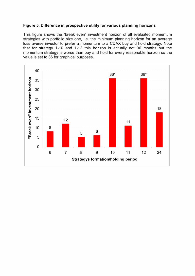
Figure 5. Difference in prospective utility for various planning horizons This figure shows the “break even” investment horizon of all evaluated momentum strategies with portfolio size one, i.e. the minimum planning horizon for an average loss averse investor to prefer a momentum to a CDAX buy and hold strategy. Note that for strategy 1-10 and 1-12 this horizon is actually not 36 months but the momentum strategy is worse than buy and hold for every reasonable horizon so the value is set to 36 for graphical purposes.

8

12

5 6

11

18

36* 36*

0

5

10

15

20

25

30

35

40

6 7 8 9 10 11 12 24

Strategys formation/holding period

"Bre

ak e

ven"

inve

stm

ent h

oriz

on

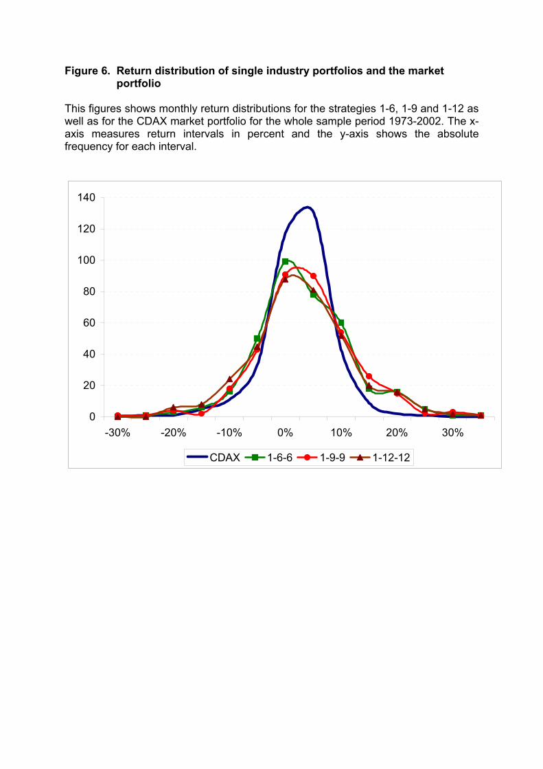
Figure 6. Return distribution of single industry portfolios and the market portfolio

This figures shows monthly return distributions for the strategies 1-6, 1-9 and 1-12 as well as for the CDAX market portfolio for the whole sample period 1973-2002. The x-axis measures return intervals in percent and the y-axis shows the absolute frequency for each interval.

0

20

40

60

80

100

120

140

-30% -20% -10% 0% 10% 20% 30%

CDAX 1-6-6 1-9-9 1-12-12

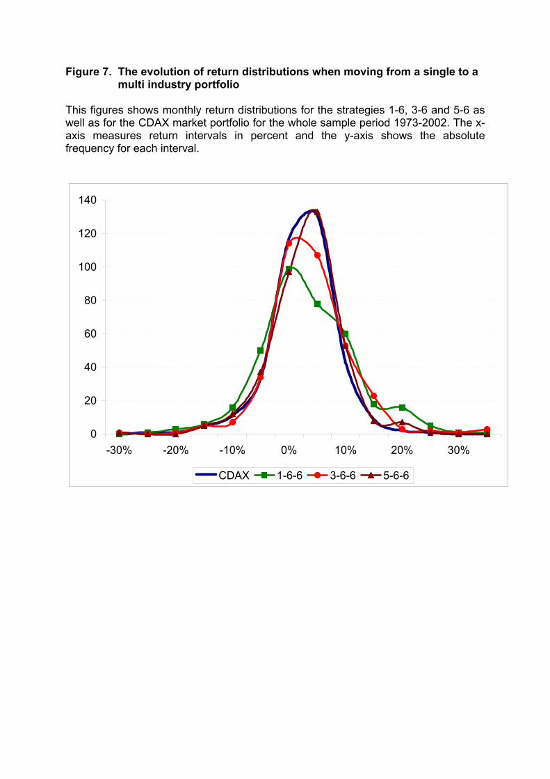
Figure 7. The evolution of return distributions when moving from a single to a multi industry portfolio

This figures shows monthly return distributions for the strategies 1-6, 3-6 and 5-6 as well as for the CDAX market portfolio for the whole sample period 1973-2002. The x-axis measures return intervals in percent and the y-axis shows the absolute frequency for each interval.

0

20

40

60

80

100

120

140

-30% -20% -10% 0% 10% 20% 30%

CDAX 1-6-6 3-6-6 5-6-6

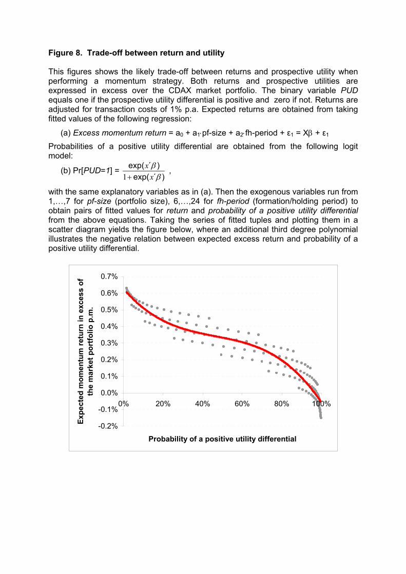
Figure 8. Trade-off between return and utility This figures shows the likely trade-off between returns and prospective utility when performing a momentum strategy. Both returns and prospective utilities are expressed in excess over the CDAX market portfolio. The binary variable PUD equals one if the prospective utility differential is positive and zero if not. Returns are adjusted for transaction costs of 1% p.a. Expected returns are obtained from taking fitted values of the following regression:

(a) Excess momentum return = a0 + a1⋅pf-size + a2⋅fh-period + ε1 = Xβ + ε1 Probabilities of a positive utility differential are obtained from the following logit model:

(b) Pr[PUD=1] = )´exp(

)´exp(β

βxx

+1 ,

with the same explanatory variables as in (a). Then the exogenous variables run from 1,…,7 for pf-size (portfolio size), 6,…,24 for fh-period (formation/holding period) to obtain pairs of fitted values for return and probability of a positive utility differential from the above equations. Taking the series of fitted tuples and plotting them in a scatter diagram yields the figure below, where an additional third degree polynomial illustrates the negative relation between expected excess return and probability of a positive utility differential.

-0.2%

-0.1%

0.0%

0.1%

0.2%

0.3%

0.4%

0.5%

0.6%

0.7%

0% 20% 40% 60% 80% 100%

Probability of a positive utility differential

Expe

cted

mom

entu

m re

turn

in e

xces

s of

th

e m

arke

t por

tfolio

p.m

.