industrial location in post-reform india: patterns of inter ...sanjoy/jds.pdfpatterns of...

Industrial Location in Post-Reform India:Patterns of Inter-regional Divergence and

Intra-regional Convergence

SANJOY CHAKRAVORTY

Where do new industrial investments locate, and what factors drivethe industrial location decisions? Do these investments follow themodel of ‘divergence followed by convergence’ suggested by thecumulative causation, agglomeration economies, and transport-costs approaches? These questions are examined with district-leveldata from India for the pre- and post-reform periods using: first,tables and maps of concentration and clustering, aggregated forall industry and disaggregated into five sectors (Heavy Industries,Chemicals and Petroleum, Textiles, Agribusiness, and Utilities),and second, logistic and OLS/Heckman selection regressionmodels for these six elements. The data provide solid evidence bothof inter-regional divergence and intra-regional convergence, andsuggest that ‘concentrated decentralisation’ is the appropriateframework for understanding industrial location in post-reformIndia.

The idea of inter-regional divergence followed by convergence is one of thecornerstones of the regional development literature. It is expected that inter-regional inequality (expressed typically in terms of per capita regionalincome or output) increases during the early years/decades of industrialdevelopment, being concentrated in metropolitan areas, and begins todecline at some later indeterminate point. This approach includes thepioneering work of Perroux [1950], Myrdal [1957], and Hirschman [1958],through the writings of Williamson [1965], Friedmann [1973], and Alonso

Sanjoy Chakravorty, Associate Professor, Department of Geography and Urban Studies, TempleUniversity, 310 Gladfelter Hall, Philadelphia, PA 19122, USA; email: [email protected]. Thisstudy was made possible through a grant from the National Science Foundation (NSF SBR9618343) and a study leave granted by Temple University. The author is indebted to Somik Lall,Michael Leeds, two anonymous referees, and to the many individuals in India who gave time andinformation. They are not, of course, responsible for anything written here.

The Journal of Development Studies, Vol.40, No.2, December 2003, pp.120–152PUBLISHED BY FRANK CASS, LONDON

402jds06.qxd 20/11/2003 10:06 20

[1980], into the contributions of new growth scholars like Krugman [1996],Sala-i-Martin [1996], and Fujita, Krugman and Venables [1999]. Thesescholars have based their work on different political, economic, andanalytical assumptions, but they have led to similar outcomes, albeit withdifferent degrees of sanguineness (Myrdal, for instance, was far less hopefulthan Hirschman about the possibility of convergence as a ‘natural’ eventualoutcome). The key to long run interregional change, in all of this literature,is the role of industrialisation, especially its spatial manifestation, or whatin the last decade or so is being called geographic concentration orclustering.1

Three main (overlapping) strands of this literature can be identified. TheHirschman and Myrdal approach can be considered under the umbrella of‘cumulative causation’, in which, ‘since nothing succeeds like success’,early industrial cities capture much of the new physical, human, andfinancial capital, often at the cost of peripheral and rural regions. This is thephase of polarisation (according to Hirschman) or backwash (according toMyrdal) and may be followed by trickle down or spread, primarily whenthere is effective political action. Perhaps the most commonly usedframework is the second strand of this literature, in which the tensionbetween agglomeration economies and diseconomies govern urban/metropolitan size, and less directly, the location of industry [Richardson,1973; Henderson, 1988].

In these export-driven models of urban and regional change, the key isnot political action, but the rise and fall of agglomeration advantages whichare derived from thick labour markets, knowledge spillovers, verticalprocess integration, and so on. The third and most recent strand of thisliterature is the most analytical and identifies transport-cost as the crucialvariable. The authors [Fujita, Krugman and Venables, 1999] build a seriesof ‘increasing returns’ models of cities, regions, and industries, where self-perpetuating forces of geographic concentration are for a time supported by,and later (in some circumstances) offset by declining transport costs. Theseinsightful models provide, for the most part, renewed analytical support forthe cumulative causation arguments made in earlier decades, and on the roleof agglomeration economies and industrial clustering.

These lines of reasoning – cumulative causation, agglomerationeconomies, or transport-cost driven ‘divergence followed by convergence’theories – presume regime or policy continuity; that is, it is taken forgranted that the regulatory conditions under which industrial locationdecisions are taken do not change. An added complication in such spatialanalytical frameworks is that the rules have recently changed. Whether ornot a ‘Washington Consensus’ or ‘Universal Convergence’ exists[Williamson, 2000], it is undeniable that over the past two decades more

121INDUSTRIAL LOCATION IN POST-REFORM INDIA

402jds06.qxd 20/11/2003 10:06 Page 121

than a hundred developing nations have undertaken structural reforms thathave liberalised their regulatory strictures on who can locate where. Theincentive and disincentive systems of the past (which notionally tended tofavour lagging, unindustrialised, non-metropolitan regions) have beenlargely discarded; the new systems profess to have little geographicalorientation, but, as many have argued, may be biased towards advanced,industrialised, metropolitan regions [Chakravorty, 2000], in other words,biased in favour of existing industrial clusters.

Conversely, Elizondo and Krugman [1992] suggest that post-reformregional industrialisation is likely to lose its historical metropolitan bias.They argue that the magnitude of internal trade is much larger than foreigntrade in inward looking trade regimes; ‘this leads to concentration ofproduction and trading activities in large metropolitan cities … an openingup of the economy is likely to break the monopoly power of these highlyconcentrated production and trading centres, weaken the traditional forwardand backward linkages and lead to a more even distribution of economicactivities across regions’ [Das and Barua, 1996: 365]. Similarly, accordingto Gilbert [1993: 729] ‘the cities which benefited most from the previousdevelopment model have suddenly had an important prop to their growthremoved’ in the new regimes of liberalisation and export orientation.

This brings us to the fundamental questions being examined in thisarticle: where do new industrial investments locate, and what forces orfactors drive the location decisions? Do these investments follow the modelof ‘divergence followed by convergence’ suggested by the cumulativecausation, agglomeration economies, and transport-costs approaches? Iexamine the questions with data from India using the 1991 reforms as thepoint of departure. The question is examined in two steps: first, I present aseries of tabular and graphical data on Indian industry, aggregated for allindustry and disaggregated into five sectors (Heavy Industries, Chemicalsand Petroleum, Textiles, Agribusiness, and Utilities). The data providesolid, if less than conclusive evidence that there is not a single definitiveanswer to the questions posed here; that is, there is evidence both ofinterregional concentration and intraregional dispersal. Second, I presenttwo sets of regression models (for all industry and the five sectors listedabove) which provide further confirmation that ‘concentrateddecentralisation’ is the appropriate framework for understanding industriallocation in the post-reform period in India.

I will dispense with any detailed discussion of India’s reforms. There isalready a large literature on the subject, on which opposing viewpoints canbe found in Byres [1997] and Joshi and Little [1997]. Dehejia [1993: 88]provides a good early summary of the extent of the reforms:

122 THE JOURNAL OF DEVELOPMENT STUDIES

402jds06.qxd 20/11/2003 10:06 Page 122

The most striking achievement of the reforms [has been] thatcommercial considerations, rather than government mandates, arenow the determinant in all investment decisions, including ownership,location, local content, technology fees, and royalty. The approvalauthority in the Directorate General of Technical Development in theMinistry of Industries has been eliminated. The Monopolies andRestrictive Practices Act has been amended … Controls on the importof capital goods have been removed, and the many regulatory bodies[have been] dissolved or reconstructed … States now compete witheach other to attract new investments.

The literature on Indian industry, which will not be referred to after thissection, tends to fall into two broad categories: (1) non-analytical, policy-oriented approaches that focus on the details of the regulatory systemgoverning Indian industrialisation. There are few works written from ageographical standpoint, being limited to descriptive approaches to regionalinequality in industrialisation or the spatial distribution of industry inspecific states or regions [Verma, 1986; Saha 1987; National Commissionon Urbanisation, 1988; Awasthi, 1991]; (2) non-spatial analysis ofindustrial productivity and growth, good examples of which are found in thewritings of Shukla [1984], Ahluwalia [1991], Becker, Williamson and Mills[1992], Das and Barua [1996] and others. There have been several empiricalestimations of production functions; for a good survey see Goldar [1997].At the end, there is little analytical information on the location of industryin India – its patterns and underlying causes, the relationships withurban/metropolitan regions – let alone any analysis of the changes inindustrial location as a result of the reforms.

DATA ISSUES

One of the primary reasons why little spatially disaggregated industrialanalysis has been undertaken in India has been the absence of appropriatedata. Indian industrial data are fairly readily available at the state level, but,for the kind of disaggregated analysis required here, state level data arevirtually useless. The two largest states, Uttar Pradesh and Bihar, beforetheir recent break-ups, had about 150 and 100 million people respectively;if independent, these would be among the largest countries in the world. Thenext largest political unit in the country is the District. There areapproximately 470 districts – the number is not fixed (just as the number ofstates is not fixed) because new districts are carved out of old ones on afairly regular basis, more so in the 1990s than ever before. Data at thedistrict level, however, have generally been unavailable.


402jds06.qxd 20/11/2003 10:06 Page 123

The Pre-Reform Data

The Central Statistical Organisation (CSO), which has the responsibility ofcollecting and disseminating most data on the Indian economy, publishesthe Annual Survey of Industries (ASI). The ASI lists sectorallydisaggregated industrial data at the state level. Though the ASI data arecollected at a smaller scale (the Block), they had never been made availableat the block or district level. The ASI covers every factory andmanufacturing unit (designated so by the Factories Act of 1948, amended in1956) using two methods: a ‘census’ sector survey with 100 per centcoverage of units employing 100 or more persons, and a ‘sample’ sectorsurvey in which a sample of the smaller units (employing between 20 and99 persons) is statistically allocated to all districts. The census sector coversover 80 per cent of the formal sector of Indian industry and is considered tobe more reliable than the sample sector. I was fortunate to be given accessto the district level data from the 1994 census sector ASI for six variables(number of factories, fixed capital, invested capital, number of employees,value of output, and net value added) at the two digit code level (that is, for29 different categories of industry). The survey on which these data arebased was carried out in 1993–94, two years after the initiation of reforms.However, since the survey covers every unit that was in operation in1993–94, whenever built, this is the most realistic measure of Indianindustry for the pre-reform period. When I refer to pre-reform data thenumbers have been derived from this data set.

Note that the ASI data have several problems. First, since the definitionof industry was set by the Factories Act, certain types of establishmentssuch as software manufacturers and everything in the service sector, are notcovered by the ASI. This is likely to affect the estimates for districts likeBangalore in Karnataka and Hyderabad in Andhra Pradesh, which byreputation at least, have attracted significant investments in the softwaresector. Second, the ASI covers only the formal sector of India’s industrialeconomy. The number of employees covered, for instance, is less than tenmillion, which clearly is a far lower number than the true size of thepopulation engaged in formal and informal industrial activity.

The Post-Reform Data

Surprisingly, no government agency has been tracking new post-reforminvestments. The economic data being generated by a private sector firm,the Center for Monitoring (the) Indian Economy (CMIE), is generallyconsidered to be the most reliable. CMIE publishes a quarterly list ofinvestment projects with markers for location (state, district, and place),project stage (completed, under implementation, seeking approvals and soon), product, capital cost and so forth. These data from 1992 to February


402jds06.qxd 20/11/2003 10:06 Page 124

1998 have been collated into a database of 4,650 records including onlythose projects that have been completed or are under implementation; it issensible to ignore the projects still in the ‘proposal’ or ‘announcement’phase as their future is quite uncertain, and those that are being fundedsolely by local government. The 1991 data were ignored as they wereunlikely to be an accurate list of ‘new’ investments; after all, the reformshad only been announced in July 1991. This database of 4,650 records orprojects covering the period 1992 through February 1998 forms the basis ofall the post-reform calculations.

The CMIE data are also likely to have problems. Primarily, it is possiblethat the CMIE’s method of data collection has introduced some bias; theirlists were compiled from official announcements (on the granting of Lettersof Intent, or the signing of Memoranda of Understanding and so on), pressreports, and company announcements and reports. This is unlikely togenerate a complete list. Second, since the CMIE is Mumbai-based, itsinformation on the west may be better than for other zones (especially thefarthest zone, the east). As a result their lists may be biased toward showingrelatively more investment in the west. But it is expected that both problemsare likely to be true for small projects (perhaps Rs 500 million or less), asbigger projects will have generated enough publicity through various mediathat they are likely to have been included in the CMIE lists.

Data Aggregation

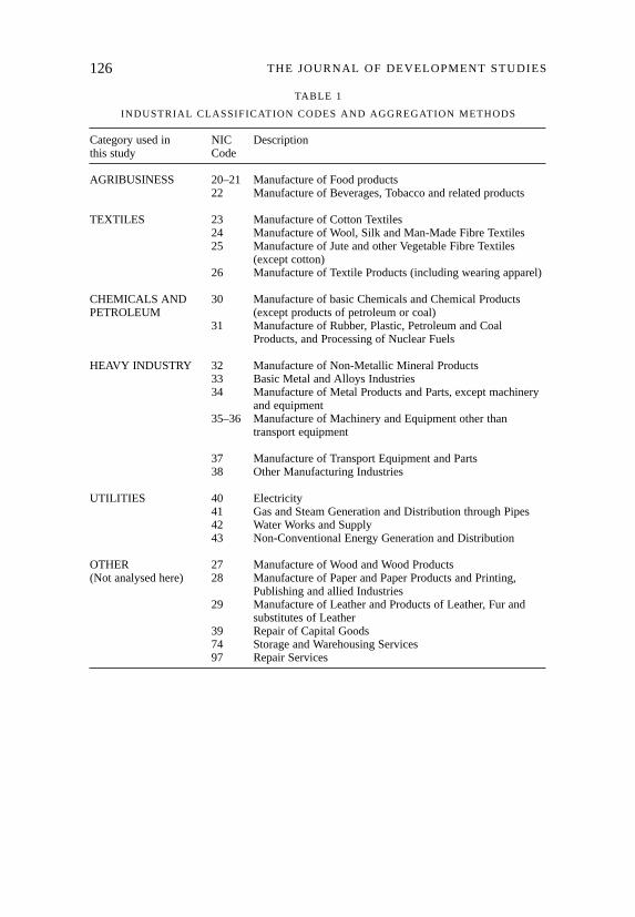
A note on the data aggregation scheme used here is necessary at this point.The ASI data were reported at the 2 digit National Industrial Classification(or NIC) code. The CMIE data are project data and have not received NICcodes yet. The two data sets were made compatible using the followingmethod: first, the ASI data, which are reported in 26 NIC 2-digit codes,were further aggregated into six sectors: Heavy Industries, Chemicals andPetroleum, Textiles, Agribusiness, Utilities, and Other (as shown in Table1). The analysis was carried out for all industry (that is, all 26 2-digit NICcategories combined together), and for the first five of the sectors identifiedhere (the ‘Other’ category, which is not internally coherent, was not used foranalysis). The ASI format was then used to assign general classificationcodes to the CMIE-listed (or post-reform) projects. In the following sectionsthe results for all industry and the five sectors are separately presentedwherever possible.2

PATTERNS OF NEW INDUSTRY LOCATION

Four sets of information are analysed in this section: Figure 1 contains mapsof post-reform investment at the district level (where investment means


402jds06.qxd 20/11/2003 10:06 Page 125


TABLE 1

INDUSTRIAL CLASSIFICATION CODES AND AGGREGATION METHODS

Category used in NIC Descriptionthis study Code

AGRIBUSINESS 20–21 Manufacture of Food products22 Manufacture of Beverages, Tobacco and related products

TEXTILES 23 Manufacture of Cotton Textiles24 Manufacture of Wool, Silk and Man-Made Fibre Textiles25 Manufacture of Jute and other Vegetable Fibre Textiles

(except cotton)26 Manufacture of Textile Products (including wearing apparel)

CHEMICALS AND 30 Manufacture of basic Chemicals and Chemical Products PETROLEUM (except products of petroleum or coal)

31 Manufacture of Rubber, Plastic, Petroleum and CoalProducts, and Processing of Nuclear Fuels

HEAVY INDUSTRY 32 Manufacture of Non-Metallic Mineral Products33 Basic Metal and Alloys Industries34 Manufacture of Metal Products and Parts, except machinery

and equipment35–36 Manufacture of Machinery and Equipment other than

transport equipment

37 Manufacture of Transport Equipment and Parts38 Other Manufacturing Industries

UTILITIES 40 Electricity41 Gas and Steam Generation and Distribution through Pipes42 Water Works and Supply43 Non-Conventional Energy Generation and Distribution

OTHER 27 Manufacture of Wood and Wood Products(Not analysed here) 28 Manufacture of Paper and Paper Products and Printing,

Publishing and allied Industries29 Manufacture of Leather and Products of Leather, Fur and

substitutes of Leather39 Repair of Capital Goods74 Storage and Warehousing Services97 Repair Services

402jds06.qxd 20/11/2003 10:06 Page 126

127IN

DU

ST

RIA

L L

OC

AT

ION

IN P

OS

T-R

EF

OR

M IN

DIA

TABLE 2

STATEWISE DISTRIBUTION OF INVESTMENT BY SELECTED SECTORS

ALL INDUSTRY HEAVY INDUSTRY CHEMICALS UTILITIES

STATE PRE- POST- PRE- POST- PRE- POST- PRE- POST-REFORM REFORM REFORM REFORM REFORM REFORM REFORM REFORMShare of Share of Share of Share of Share of Share of Share of Share ofNational National National National National National National NationalTotal (%) Total (%) Total (%) Total (%) Total (%) Total (%) Total (%) Total (%)

ANDHRA PRADESH (AP) 8.85 6.22 11.30 5.29 6.04 5.81 9.32 8.63ASSAM (ASS) 0.75 2.19 0.14 0.12 1.28 4.98 0.03 1.47BIHAR (BIH) 6.09 3.74 12.24 7.33 2.04 0.90 4.81 3.04CHANDIGARH (CHN) 0.03 0.05 0.03 0.10 0.00 0.00 0.00 0.00DADRA & NAGAR HAVELI 0.09 0.25 0.26 0.31 0.03 0.09 0.00 0.00DELHI (DLH) 1.00 0.15 0.70 0.03 0.08 0.03 1.46 0.07GOA 0.29 0.27 0.22 0.44 0.61 0.13 0.07 0.16GUJARAT (GUJ) 10.05 16.89 5.60 7.80 24.43 30.07 6.84 14.98HARYANA (HAR) 2.53 2.36 4.25 2.63 0.48 3.11 1.86 1.03HIMACHAL PRADESH (HP) 0.79 1.33 0.52 0.71 0.16 0.06 1.33 3.10KARNATAKA (KAR) 3.66 7.17 4.96 8.69 1.29 2.76 3.02 10.02KERALA (KER) 1.96 1.30 0.72 0.68 3.57 1.53 2.46 2.13MADHYA PRADESH (MP) 6.33 7.94 8.86 11.66 3.37 5.78 5.85 4.99MAHARASHTRA (MAH) 18.11 13.44 16.42 14.98 24.05 13.89 14.59 10.07ORISSA (ORI) 4.67 5.96 7.12 11.85 2.08 1.19 5.45 4.60PONDICHERRY (PON) 0.21 0.37 0.27 0.20 0.22 1.04 0.00 0.02PUNJAB (PUN) 3.86 3.94 2.16 1.57 2.25 6.73 5.50 0.32RAJASTHAN (RAJ) 3.89 3.71 3.30 4.02 4.05 0.97 3.88 5.75TAMIL NADU (TN) 8.48 8.71 5.27 9.46 9.51 8.38 9.03 9.61TRIPURA (TRI) 0.03 0.10 0.01 0.04 0.00 0.00 0.08 0.33UTTAR PRADESH (UP) 10.68 8.15 5.39 6.32 10.07 8.13 15.67 11.04WEST BENGAL (WB) 7.30 5.64 10.16 5.59 4.05 4.43 8.17 8.24

Source: Own calculations from the ASI and CMIE data (discussed in text).

402jds06.qxd 20/11/2003 10:06 Page 127

128T

HE

JOU

RN

AL

OF

DE

VE

LO

PM

EN

T S

TU

DIE

S

TABLE 3

TOP 25 DISTRICTS AND THEIR SHARES

ALL INDUSTRY HEAVY INDUSTRY

PRE-REFORM POST-REFORM PRE-REFORM POST-REFORM

1 Greater Bombay MAH 8.23 Bharuch GUJ 4.29 Vishakhapatnam AP 7.61 Barddhaman WB 3.952 Vadodara GUJ 3.90 Surat GUJ 4.28 Barddhaman WB 7.50 Raigarh MAH 3.933 Lucknow UP 3.71 Jamnagar GUJ 3.55 Purbi Singhbhum BIH 6.73 Ganjam ORI 3.554 Vishakhapatnam AP 2.93 Chengaianna TN 3.45 Pune MAH 5.02 Chengaianna TN 3.455 Barddhaman WB 2.74 Raigarh MAH 2.82 Sundargarh ORI 4.42 Pune MAH 3.436 Madras TN 2.48 Greater Bombay MAH 2.75 Greater Bombay MAH 4.26 Dakshin Kannad KAR 2.897 Pune MAH 2.34 Dakshin Kannad KAR 2.57 Dhanbad BIH 4.08 Raipur MP 2.678 Hyderabad AP 2.31 Vishakhapatnam AP 2.06 Durg MP 2.98 Koraput ORI 2.639 Purbi Singhbhum BIH 2.26 South Arcot TN 2.00 Bangalore KAR 2.56 Bellary KR 2.62

10 Patiala PUN 1.81 Ratnagiri MAH 1.80 Gurgaon HAR 1.83 Ghaziabad UP 2.56

Top 10 Total 32.71 Top 10 Total 29.58 Top 10 Total 46.99 Top 10 Total 31.68

11 Raigarh MAH 1.80 Ghaziabad UP 1.75 Chengaianna TN 1.52 Surat GUJ 2.5012 Bangalore KAR 1.79 Bhatinda PUN 1.68 Raigarh MAH 1.27 Purbi Singhbhum BIH 2.3813 Jabalpur MP 1.67 Pune MAH 1.61 Faridabad HAR 1.24 Sundargarh ORI 2.1414 Surat GUJ 1.66 Thane MAH 1.61 Surat GUJ 1.21 Dhanbad BIH 1.8615 Chengaianna TN 1.52 Barddhaman WB 1.52 Aurangabad MAH 1.21 Gurgaon HAR 1.8416 Sundargarh ORI 1.50 Bellary KAR 1.39 Bharuch GUJ 1.20 Bharuch GUJ 1.7617 N. 24 Parganas WB 1.50 Ganjam ORI 1.36 Ghaziabad UP 1.19 South Arcot TN 1.6718 Dhanbad BIH 1.44 Medinipur WB 1.35 Thane MAH 1.14 Durg MP 1.5719 Sonbhadra UP 1.38 Vadodara GUJ 1.34 Salem AP 1.03 Ratnagiri MAH 1.4720 Dhenkanal ORI 1.36 Sagar MP 1.15 Sonbhadra UP 0.95 Kedunjhar ORI 1.3621 Thane MAH 1.33 Cuttack ORI 1.11 Bilaspur MP 0.91 Gulbarga KAR 1.2422 Bharuch GUJ 1.20 Dibrugarh ASS 1.04 Medak AP 0.90 Vishakhapatnam AP 1.1523 Jaipur RAJ 1.17 Purbi Singhbhum BIH 1.04 Raipur MP 0.85 Kachchh GUJ 1.1424 Durg MP 1.02 Raipur MP 1.03 Chittaurgarh RAJ 0.81 Thane MAH 1.1125 Ahmadabad GUJ 0.90 Koraput ORI 0.98 Nagpur MAH 0.80 Sidhi 1.08

Top 25 Total: 53.95 Top 25 Total: 49.53 Top 25 Total: 63.22 Top 25 Total: 55.94

402jds06.qxd 20/11/2003 10:06 Page 128

129IN

DU

ST

RIA

L L

OC

AT

ION

IN P

OS

T-R

EF

OR

M IN

DIA

1 Vadodara GUJ 12.41 Jamnagar GUJ 12.36 Greater Bombay MAH 14.47 Surat GUJ 7.162 Greater Bombay MAH 8.17 Bharuch GUJ 7.81 Lucknow UP 11.98 Bharuch GUJ 4.253 Raigarh MAH 7.14 Greater Bombay MAH 7.01 Madras TN 7.48 Thane MAH 4.214 Chengaianna TN 4.68 Bhatinda PUN 6.23 Hyderabad AP 7.27 Dakshin Kannad KAR 3.635 Thane MAH 3.94 Chengaianna TN 5.43 Patiala PUN 5.49 Garhwal UP 3.286 Bharuch GUJ 3.85 Sagar MP 4.26 Jabalpur MP 5.35 South Arcot TN 2.977 Ernakulam KER 2.88 Surat GUJ 4.21 Vadodara GUJ 4.74 Vishakhapatnam AP 2.878 Kota RAJ 2.61 Medinipur WB 4.11 N. 24 Parganas WB 3.49 East Godavari AP 2.419 Budaun UP 2.47 Vishakhapatnam AP 3.44 Dhenkanal ORI 3.34 Ghaziabad UP 2.18

10 East Godavari AP 2.19 Vadodara GUJ 2.89 Jaipur RAJ 3.31 Chengaianna TN 2.16

Top 10 Total 50.33 Top 10 Total 57.75 Top 10 Total 66.93 Top 10 Total 35.10

11 Pune MAH 2.18 Ratnagiri MAH 2.89 Sonbhadra UP 3.27 Murshidabad WB 2.0812 Surat GUJ 2.05 Raigarh MAH 2.83 Murshidabad WB 2.84 Sidhi MP 2.0113 Vishakhapatnam AP 1.92 Dibrugarh ASS 2.65 Thiruvananthapuram TN 2.43 Ratnagiri MAH 1.9014 Chidambaranar TN 1.86 Panipat HAR 2.40 Patna BIH 2.19 Cuttack ORI 1.8515 Cuttack ORI 1.40 South Arcot TN 2.29 Bangalore KAR 2.01 Greater Bombay MAH 1.6216 Jamnagar GUJ 1.35 Dakshin Kannad KAR 2.14 Karimnagar AP 2.00 Tirunelveli TN 1.5717 Junagadh GUJ 1.25 Mathura UP 1.52 Gaya BIH 1.88 Rai Bareli UP 1.5318 Mahesana GUJ 1.21 Ernakulam KER 1.50 Ambala HAR 1.82 Uttar Kannad KAR 1.5119 Medinipur WB 1.15 Etawah UP 1.47 South Arcot TN 1.53 Madras TN 1.4720 Mathura UP 1.13 Sibsagar ASS 1.30 Surat GUJ 1.52 Raigarh MAH 1.4321 Valsad GUJ 1.12 Cuttack ORI 1.05 Medinipur WB 1.30 Dholpur RAJ 1.4322 Hugli WB 1.02 Nellore AP 1.01 Puri ORI 1.24 S. 24 Parganas WB 1.3623 Nilgiri TN 1.00 Shahjahanpur UP 0.84 Shimla HP 1.18 Dibrugarh ASS 1.3624 Moradabad UP 0.91 Kachchh GUJ 0.77 Ahmadabad GUJ 0.58 Chamba HP 1.3525 Bhind MP 0.88 Bareilly UP 0.76 Raichur KAR 0.58 Hugli WB 1.34

Top 25 Total: 70.77 Top 25 Total: 83.20 Top 25 Total: 93.31 Top 25 Total: 58.91

Source: Own calculations from the ASI and CMIE data (discussed in text).

TABLE 3 (Cont’d)

CHEMICALS AND PETROLEUM UTILITIES

PRE-REFORM POST-REFORM PRE-REFORM POST-REFORM

402jds06.qxd 20/11/2003 10:06 Page 129

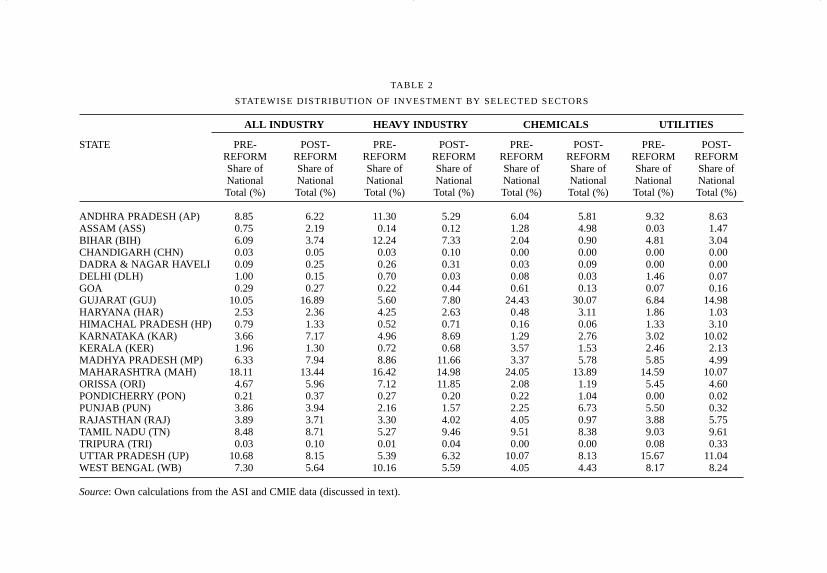
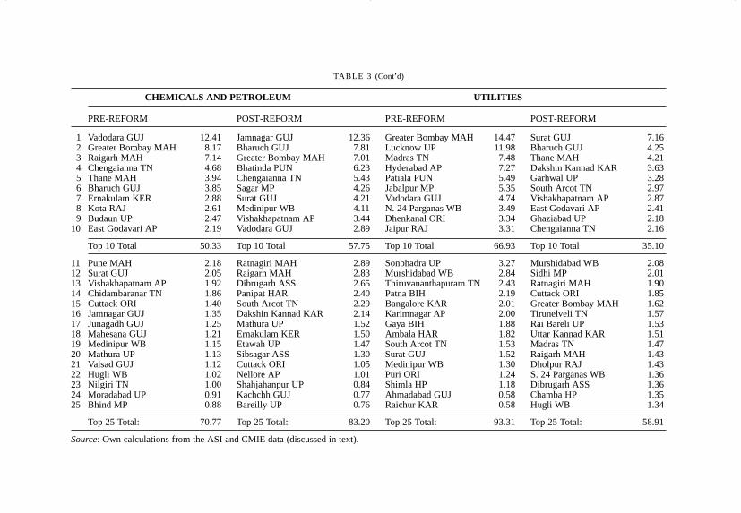
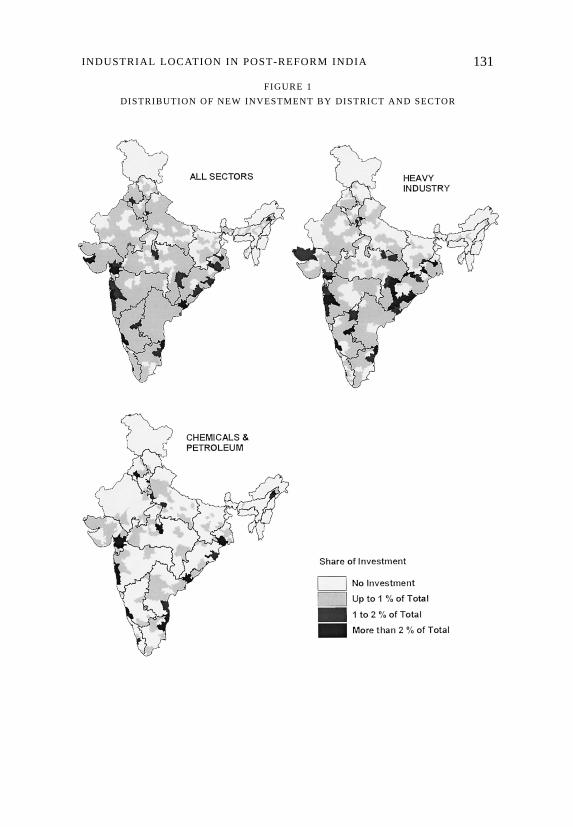
‘invested capital’ from the ASI or pre-reform data, and project cost from theCMIE or post-reform data).3 Table 2 contains data on pre- and post-reforminvestment at the state level.4 Table 3 lists the investment data for the topdistricts. Table 4 shows the results of calculations for industry concentrationand clustering.

Investments at the State Level

Let us begin at the state level with pre- and post-reform investment data forall industry, and the Heavy Industries, Chemicals and Utilities sectors asreported in Table 2 and mapped in Figure 1. The maps provide an earlyindication of the spatial distribution of new industry. We see theconcentration of industry on the west and east coasts, and the sparseness ofindustry in Bihar, eastern Uttar Pradesh, and central Madhya Pradesh. Thisbasic pattern is confirmed in the sectoral maps, especially the absence of


TABLE 4

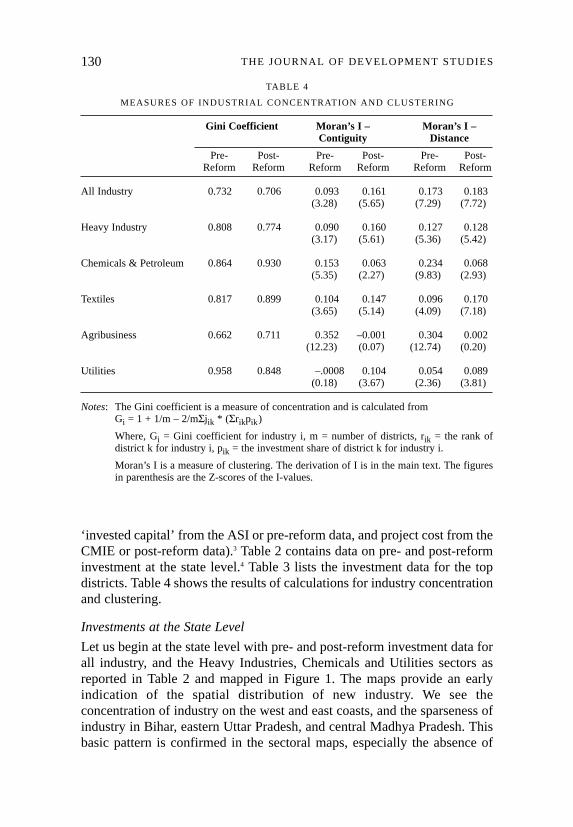
MEASURES OF INDUSTRIAL CONCENTRATION AND CLUSTERING

Gini Coefficient Moran’s I – Moran’s I –Contiguity Distance

Pre- Post- Pre- Post- Pre- Post-Reform Reform Reform Reform Reform Reform

All Industry 0.732 0.706 0.093 0.161 0.173 0.183(3.28) (5.65) (7.29) (7.72)

Heavy Industry 0.808 0.774 0.090 0.160 0.127 0.128(3.17) (5.61) (5.36) (5.42)

Chemicals & Petroleum 0.864 0.930 0.153 0.063 0.234 0.068(5.35) (2.27) (9.83) (2.93)

Textiles 0.817 0.899 0.104 0.147 0.096 0.170(3.65) (5.14) (4.09) (7.18)

Agribusiness 0.662 0.711 0.352 –0.001 0.304 0.002(12.23) (0.07) (12.74) (0.20)

Utilities 0.958 0.848 –.0008 0.104 0.054 0.089(0.18) (3.67) (2.36) (3.81)

Notes: The Gini coefficient is a measure of concentration and is calculated fromGi = 1 + 1/m – 2/mΣjik * (Σrikpik)

Where, Gi = Gini coefficient for industry i, m = number of districts, rik = the rank ofdistrict k for industry i, pik = the investment share of district k for industry i.

Moran’s I is a measure of clustering. The derivation of I is in the main text. The figuresin parenthesis are the Z-scores of the I-values.

402jds06.qxd 20/11/2003 10:06 Page 130


FIGURE 1

DISTRIBUTION OF NEW INVESTMENT BY DISTRICT AND SECTOR

402jds06.qxd 20/11/2003 10:06 Page 131


FIGURE 1 (Cont’d)

402jds06.qxd 20/11/2003 10:06 2

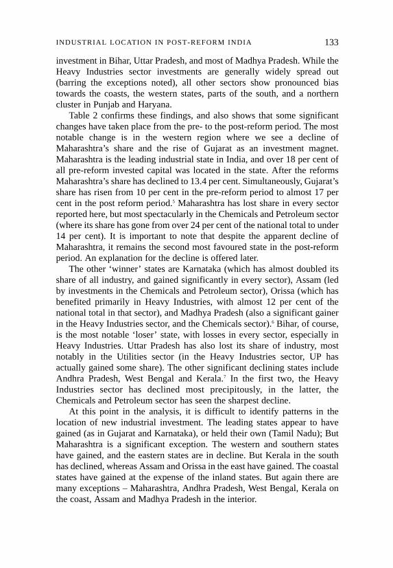
investment in Bihar, Uttar Pradesh, and most of Madhya Pradesh. While theHeavy Industries sector investments are generally widely spread out(barring the exceptions noted), all other sectors show pronounced biastowards the coasts, the western states, parts of the south, and a northerncluster in Punjab and Haryana.

Table 2 confirms these findings, and also shows that some significantchanges have taken place from the pre- to the post-reform period. The mostnotable change is in the western region where we see a decline ofMaharashtra’s share and the rise of Gujarat as an investment magnet.Maharashtra is the leading industrial state in India, and over 18 per cent ofall pre-reform invested capital was located in the state. After the reformsMaharashtra’s share has declined to 13.4 per cent. Simultaneously, Gujarat’sshare has risen from 10 per cent in the pre-reform period to almost 17 percent in the post reform period.5 Maharashtra has lost share in every sectorreported here, but most spectacularly in the Chemicals and Petroleum sector(where its share has gone from over 24 per cent of the national total to under14 per cent). It is important to note that despite the apparent decline ofMaharashtra, it remains the second most favoured state in the post-reformperiod. An explanation for the decline is offered later.

The other ‘winner’ states are Karnataka (which has almost doubled itsshare of all industry, and gained significantly in every sector), Assam (ledby investments in the Chemicals and Petroleum sector), Orissa (which hasbenefited primarily in Heavy Industries, with almost 12 per cent of thenational total in that sector), and Madhya Pradesh (also a significant gainerin the Heavy Industries sector, and the Chemicals sector).6 Bihar, of course,is the most notable ‘loser’ state, with losses in every sector, especially inHeavy Industries. Uttar Pradesh has also lost its share of industry, mostnotably in the Utilities sector (in the Heavy Industries sector, UP hasactually gained some share). The other significant declining states includeAndhra Pradesh, West Bengal and Kerala.7 In the first two, the HeavyIndustries sector has declined most precipitously, in the latter, theChemicals and Petroleum sector has seen the sharpest decline.

At this point in the analysis, it is difficult to identify patterns in thelocation of new industrial investment. The leading states appear to havegained (as in Gujarat and Karnataka), or held their own (Tamil Nadu); ButMaharashtra is a significant exception. The western and southern stateshave gained, and the eastern states are in decline. But Kerala in the southhas declined, whereas Assam and Orissa in the east have gained. The coastalstates have gained at the expense of the inland states. But again there aremany exceptions – Maharashtra, Andhra Pradesh, West Bengal, Kerala onthe coast, Assam and Madhya Pradesh in the interior.


402jds06.qxd 20/11/2003 10:06 Page 133

Investments at the District Level

The district level data in Table 3 begin to offer some explanation. Here thetop districts and their investment shares are identified for the pre- and post-reform periods for all industry, and the Heavy Industries, Chemicals andPetroleum, and Utilities sectors. The figures indicate a significant change inlocation patterns. There are three important patterns revealed in this list:

(1) The decline of metropolitan districts: Consider the category of allindustry. Only two of the top ten districts from the pre-reform period havemanaged to remain in the top ten in the post-reform period. These areGreater Bombay and Vishakhapatnam, both of which have lost share in thetransition. Greater Bombay’s experience is illuminating: it was by far theleading district in the country in the pre-reform period (with 8.23 per centof the national fixed capital); after the reforms it is ranked sixth, with 2.75per cent of the national total. Greater Bombay has gone from sixth on thepre-reform Heavy Industries list to out of the list altogether in the post-reform period (similar to what has happened to Bangalore district); it hasgone from second to third in Chemicals and Petroleum, and from first tofifteenth in Utilities. Greater Bombay’s loss more than accounts forMaharashtra’s total loss; in fact, ignoring Greater Bombay, the rest ofMaharashtra has actually seen an increase in its share of investment. This isan important development that explains the apparent investment decline inthe state. At the same time, some pre-reform top ten districts have droppedout of the post-reform top 25 list: these are Lucknow, Madras, Hyderabad,and Patiala, all urban districts with two being the central city districts of thefourth and fifth largest metropolises in India.

(2) The continuing decline of the inland region: Every district in the allindustry post-reform top ten lies to the south of the Vindhyas, the somewhatimaginary line dividing north and south India. Uttar Pradesh and Bihar, thetwo largest and also landlocked states in the country, together account for aquarter of India’s population, yet have only one district each in the post-reform all industry top 25: Ghaziabad (at rank 11) in Uttar Pradesh, whichis part of the Delhi metropolis, and Purbi Singhbhum (at rank 23), themanufacturing base of the giant Tata group. The post-reform HeavyIndustries list contains these two and Dhanbad, the center of the coalindustry. The Chemicals and Utilities lists are similarly sparsely populatedwith inland districts.

(3) The rise of non-metropolitan areas: Greater Bombay, Madras, Delhi,Hyderabad, Ahmadabad, Bangalore, Lucknow, etc. have all declined;Calcutta has improved marginally but from an extremely poor position and


402jds06.qxd 20/11/2003 10:06 Page 134

still cannot come close to breaking into the top 25 list. In contrast, somesuburban districts have risen – such as Chengaianna (surrounding Madras),and Raigarh and Thane (around Bombay). But the most impressiveperformance has been shown by non-metropolitan, even non-urban districtssuch as Bharuch, Jamnagar, Dakshin Kannad, South Arcot, Surat,Medinipur, etc. These names are not completely new – Raigarh,Chengaianna, Surat, Bharuch, and Medinipur were already in the top 25earlier (which is to suggest that the emergence of these districts is notentirely a result of the reforms).

This list shows the emergence of India’s new industrial core – a leadingedge of non-metropolitan, coastal districts that are relatively proximate tometropolitan areas. The most important of these clusters is the corridorstretching from south of Greater Bombay northward into southern Gujarat,and includes the districts of Ratnagiri, Raigarh, Greater Bombay, Pune,Thane (all in Maharashtra), and Bharuch, Surat, and Vadodara (all inGujarat). The Mumbai metropolis is the anchor of this coastal industrialcluster which has heavy concentrations of Heavy Industry, Chemicals andPetroleum, and Utilities. The second major cluster is in the districts around(but not in) Madras district in Tamil Nadu state, where the prime attractorsof new investment are Chengaianna and South Arcot districts. In otherwords, industrial growth has spread outwards from some (Mumbai andChennai) of the existing core industrial districts (which in turn havedeclined), but not from others (Calcutta); it has also continued in some non-metropolitan centres of heavy industry (Barddhaman and Vishakhapatnam,both with large public sector investments), and found new non-industriallocations (Ganjam in Orissa, Dakshin Kannad in Karnataka). That is, thereis evidence both of clustering and dispersal of new industrial investments.

Concentration and Clustering at the District Level

Table 3 also provides some information on the extent of investmentconcentration in the top districts. The share of all industry investmentsconcentrated in the top ten or top 25 districts is quite consistent over the twoperiods. The level of concentration is very high: the top ten districts attractabout one-third and the top 25 districts attract about one-half of totalinvestment in the country in both periods; not unexpectedly, the shares inthe top districts in the other sectors – Heavy Industries, Utilities, andChemicals – are even higher.

These lists, while informative, do not include the full distribution ofinvestments, neither is it possible to make summary judgments on the extentof concentration or clustering or change in either dimension. There is anemerging literature on industry concentration and its relationship toagglomeration, trade, and growth. This area has long been of interest to


402jds06.qxd 20/11/2003 10:06 Page 135

urban geographers and urban economists, and over the past decade hasreceived renewed interest following the work of Krugman [1991; alsoEllison and Glaeser, 1997; Rosenthal and Strange, 2001]. Several devicesto measure industry concentration have been discovered or rediscovered.Prominent among these are the ‘spatial Gini’ and Ellison and Glaeser’s γ.These measures suffer from a common drawback, one that White [1983]termed the ‘checkerboard problem’, whereby these measures are not reallyspatial – any geographical arrangement of parcels (in this case districts)would yield the same measure of concentration. Hence ‘concentration’ hasto be distinguished from ‘clustering’ where the latter is explicitly spatial;that is, geographical arrangements are incorporated in measures ofclustering, which is a case of ‘spatial autocorrelation’.

A note on spatial autocorrelation is necessary here. This is useful forunderstanding measures of clustering and for the ‘spatial lag’ term used inthe models in the following section. The feature of spatial distributions inwhich proximate phenomena tend to be similar is called spatialautocorrelation; this is positive when like values cluster together (that is,high values are proximate to high values, and low values are proximate tolow values) which is a clear expectation of geographers, or negative (whenhigh and low values are proximate) which is rare and difficult to explain. Inregression modelling, spatial autocorrelation creates problems similar tothose caused by multicollinearity: the estimates are biased. Therefore whenspatial autocorrelation exists corrective steps must be taken. One of theways of dealing with the spatial autocorrelation problem in a regressionmodelling format is to add a ‘spatial lag’ term on the right hand side.According to Anselin [1992: 18–1] ‘spatial lag is a weighted average of thevalues in locations neighboring each observation … if an observation onvariable x at location i is represented by xi, then its spatial lag is Σj wijxj’,which is the sum of the product of each observation in the data set with itscorresponding spatial weight.

Moran’s I is a measure of spatial autocorrelation and therefore can alsobe used as a measure of clustering. It is given by

I = m/S0 ΣiΣj wij.(xi-µ).(xj-µ) / Σi (xi-µ)2 (1)

where, wij is the element in the spatial weights matrix corresponding to theobservation pair i,j; xi and xj are observations (investments) for locations iand j (with mean µ); and S0 is a scaling constant (that is, the sum of allspatial weights). For Moran’s I – Contiguity, the weights matrix assigns aweight of 1 to all j that are contiguous to i (that are direct neighbours), anda weight of 0 to all other j. For Moran’s I – Distance, the weights matrixassigns a value of 1 to all j that are within a chosen critical distance of x,and a value of 0 to all other j. 150 kilometres is the critical distance in this


402jds06.qxd 20/11/2003 10:06 Page 136

case, that is, all districts whose centroids lie within 150 kilometres of thecentroid of district x are assigned a spatial weight of 1.

The summary measures reported in Table 4 use the Gini coefficient tomeasure concentration (γ was also calculated, but since the number ofobservations is high, it is virtually indistinguishable from the Gini), andMoran’s I to measure clustering. The results are very interesting. In general,concentration and clustering processes have moved in opposite directions.Concentration has declined for all industry, Heavy Industry, and Utilities,and it has increased for Chemicals and Petroleum, Textiles, andAgribusiness. Clustering has increased for all but Chemicals andAgribusiness; for the latter, there is no evidence of clustering in the post-reform data.8 The Textiles sector is the only one where both measures havemoved in the same, higher direction. Consider the implications of thegeneral finding by looking at one instance, say Heavy Industry. The declinein concentration is to be expected from the data in Table 3. The top districtshave lost share, therefore lower ranked districts have higher shares thanbefore. The increase in clustering suggests that the spread of Heavy Industryinvestment is greatest in adjacent or proximate districts. In other words, thenew investments are spatially more concentrated than before. Later, afterfurther evidence from the modeling exercise below, I will discuss thesefindings in terms of ‘concentrated decentralisation’.

EXPLANATORY MODELS OF NEW INDUSTRY LOCATION

What are the factors that contribute to the location decision of new industry?This article began with the suggestion that concentration processes areimportant in the location decision. This implies that new industrialinvestments are likely to be located near existing industrial investments. Notonly that, but new investments are likely to be near locations where othernew investments are being made. That is, concentration and clustering areexpressed through investments: existing or old investments, and newinvestments in proximate or surrounding areas respectively. In addition,some locations have advantages deriving from capital availability andcapital productivity, labour availability, labour skills and labourproductivity, physical and social infrastructure, political support, and spatialphenomena such as access to consumer markets and coastal regions[Hoover, 1968; Chapman and Walker, 1991; Harrington and Warf, 1995].Hence a model of the following form may be specified:

Inew = f(Iold, Ilag, K, L, I, P, S) (2)

where,Inew, Iold, and Ilag are the log transformations of new investment, existing


402jds06.qxd 20/11/2003 10:06 Page 137

investment, and spatial lag of new investment respectively. Note that thesevariables take different sets of values depending upon the sector beinganalysed; that is, when all industry is under consideration, Inew, Iold, and Ilagare those for all industry investments only. The same condition applies toeach of the five other sectors being analysed.

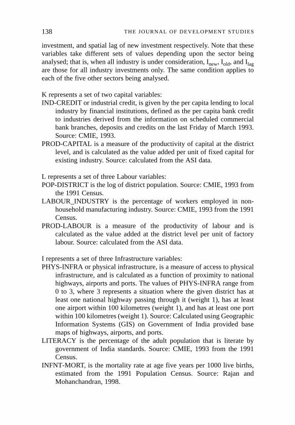
K represents a set of two capital variables:IND-CREDIT or industrial credit, is given by the per capita lending to local

industry by financial institutions, defined as the per capita bank creditto industries derived from the information on scheduled commercialbank branches, deposits and credits on the last Friday of March 1993.Source: CMIE, 1993.

PROD-CAPITAL is a measure of the productivity of capital at the districtlevel, and is calculated as the value added per unit of fixed capital forexisting industry. Source: calculated from the ASI data.

L represents a set of three Labour variables:POP-DISTRICT is the log of district population. Source: CMIE, 1993 from

the 1991 Census.LABOUR_INDUSTRY is the percentage of workers employed in non-

household manufacturing industry. Source: CMIE, 1993 from the 1991Census.

PROD-LABOUR is a measure of the productivity of labour and iscalculated as the value added at the district level per unit of factorylabour. Source: calculated from the ASI data.

I represents a set of three Infrastructure variables:PHYS-INFRA or physical infrastructure, is a measure of access to physical

infrastructure, and is calculated as a function of proximity to nationalhighways, airports and ports. The values of PHYS-INFRA range from0 to 3, where 3 represents a situation where the given district has atleast one national highway passing through it (weight 1), has at leastone airport within 100 kilometres (weight 1), and has at least one portwithin 100 kilometres (weight 1). Source: Calculated using GeographicInformation Systems (GIS) on Government of India provided basemaps of highways, airports, and ports.

LITERACY is the percentage of the adult population that is literate bygovernment of India standards. Source: CMIE, 1993 from the 1991Census.

INFNT-MORT, is the mortality rate at age five years per 1000 live births,estimated from the 1991 Population Census. Source: Rajan andMohanchandran, 1998.


402jds06.qxd 20/11/2003 10:06 Page 138

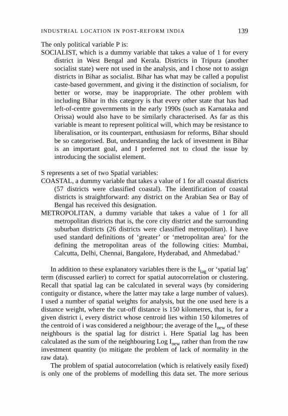
The only political variable P is:SOCIALIST, which is a dummy variable that takes a value of 1 for every

district in West Bengal and Kerala. Districts in Tripura (anothersocialist state) were not used in the analysis, and I chose not to assigndistricts in Bihar as socialist. Bihar has what may be called a populistcaste-based government, and giving it the distinction of socialism, forbetter or worse, may be inappropriate. The other problem withincluding Bihar in this category is that every other state that has hadleft-of-centre governments in the early 1990s (such as Karnataka andOrissa) would also have to be similarly characterised. As far as thisvariable is meant to represent political will, which may be resistance toliberalisation, or its counterpart, enthusiasm for reforms, Bihar shouldbe so categorised. But, understanding the lack of investment in Biharis an important goal, and I preferred not to cloud the issue byintroducing the socialist element.

S represents a set of two Spatial variables:COASTAL, a dummy variable that takes a value of 1 for all coastal districts

(57 districts were classified coastal). The identification of coastaldistricts is straightforward: any district on the Arabian Sea or Bay ofBengal has received this designation.

METROPOLITAN, a dummy variable that takes a value of 1 for allmetropolitan districts that is, the core city district and the surroundingsuburban districts (26 districts were classified metropolitan). I haveused standard definitions of ‘greater’ or ‘metropolitan area’ for thedefining the metropolitan areas of the following cities: Mumbai,Calcutta, Delhi, Chennai, Bangalore, Hyderabad, and Ahmedabad.9

In addition to these explanatory variables there is the Ilag or ‘spatial lag’term (discussed earlier) to correct for spatial autocorrelation or clustering.Recall that spatial lag can be calculated in several ways (by consideringcontiguity or distance, where the latter may take a large number of values).I used a number of spatial weights for analysis, but the one used here is adistance weight, where the cut-off distance is 150 kilometres, that is, for agiven district i, every district whose centroid lies within 150 kilometres ofthe centroid of i was considered a neighbour; the average of the Inew of theseneighbours is the spatial lag for district i. Here Spatial lag has beencalculated as the sum of the neighbouring Log Inew rather than from the rawinvestment quantity (to mitigate the problem of lack of normality in theraw data).

The problem of spatial autocorrelation (which is relatively easily fixed)is only one of the problems of modelling this data set. The more serious


402jds06.qxd 20/11/2003 10:06 Page 139

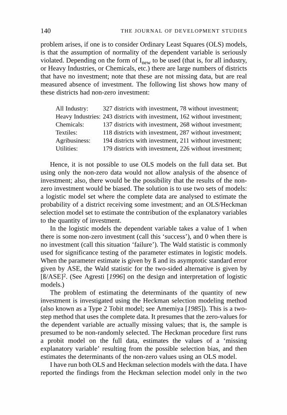
problem arises, if one is to consider Ordinary Least Squares (OLS) models,is that the assumption of normality of the dependent variable is seriouslyviolated. Depending on the form of Inew to be used (that is, for all industry,or Heavy Industries, or Chemicals, etc.) there are large numbers of districtsthat have no investment; note that these are not missing data, but are realmeasured absence of investment. The following list shows how many ofthese districts had non-zero investment:

All Industry: 327 districts with investment, 78 without investment;Heavy Industries: 243 districts with investment, 162 without investment;Chemicals: 137 districts with investment, 268 without investment;Textiles: 118 districts with investment, 287 without investment;Agribusiness: 194 districts with investment, 211 without investment;Utilities: 179 districts with investment, 226 without investment;

Hence, it is not possible to use OLS models on the full data set. Butusing only the non-zero data would not allow analysis of the absence ofinvestment; also, there would be the possibility that the results of the non-zero investment would be biased. The solution is to use two sets of models:a logistic model set where the complete data are analysed to estimate theprobability of a district receiving some investment; and an OLS/Heckmanselection model set to estimate the contribution of the explanatory variablesto the quantity of investment.

In the logistic models the dependent variable takes a value of 1 whenthere is some non-zero investment (call this ‘success’), and 0 when there isno investment (call this situation ‘failure’). The Wald statistic is commonlyused for significance testing of the parameter estimates in logistic models.When the parameter estimate is given by ß and its asymptotic standard errorgiven by ASE, the Wald statistic for the two-sided alternative is given by[ß/ASE]2. (See Agresti [1996] on the design and interpretation of logisticmodels.)

The problem of estimating the determinants of the quantity of newinvestment is investigated using the Heckman selection modeling method(also known as a Type 2 Tobit model; see Amemiya [1985]). This is a two-step method that uses the complete data. It presumes that the zero-values forthe dependent variable are actually missing values; that is, the sample ispresumed to be non-randomly selected. The Heckman procedure first runsa probit model on the full data, estimates the values of a ‘missingexplanatory variable’ resulting from the possible selection bias, and thenestimates the determinants of the non-zero values using an OLS model.

I have run both OLS and Heckman selection models with the data. I havereported the findings from the Heckman selection model only in the two


402jds06.qxd 20/11/2003 10:06 Page 140

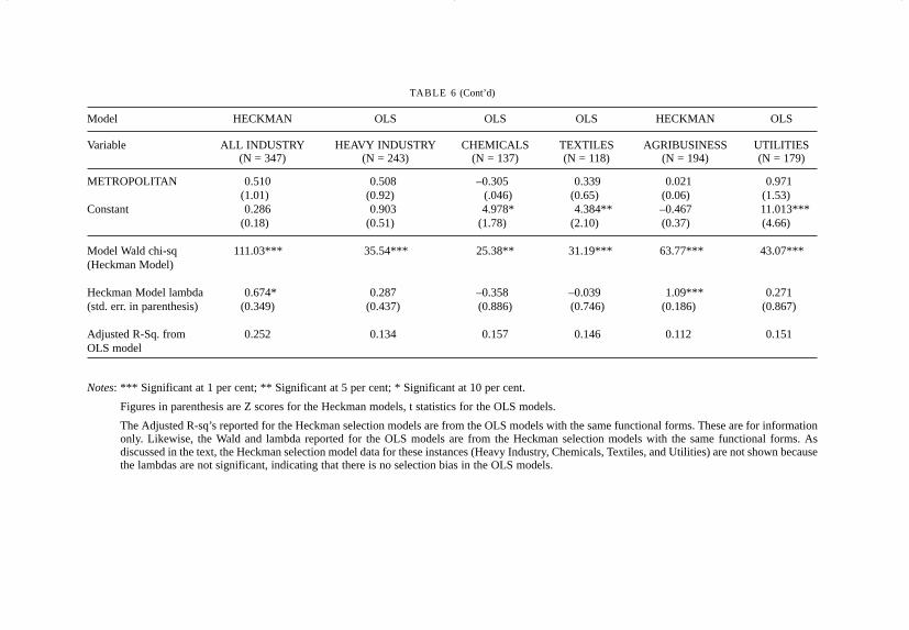
cases (all industry and Agribusiness) with significant selection bias(indicated by the estimates of lambda, a model statistic reported for all themodels). I have also reported the OLS generated adjusted R-square valuesfor all models to indicate their predictive ability; hence, in the two caseswhere the Heckman selection estimates are reported, the adjusted R-squarefigures are from the corresponding OLS model. It is to be noted that that theHeckman selection parameter estimates, even in the two cases where thereis selection bias, are virtually identical to the OLS estimates. Good surveysof the Heckman two-stage estimation process are in Vella [1998] andWinship and Mare [1992].

MODEL FINDINGS

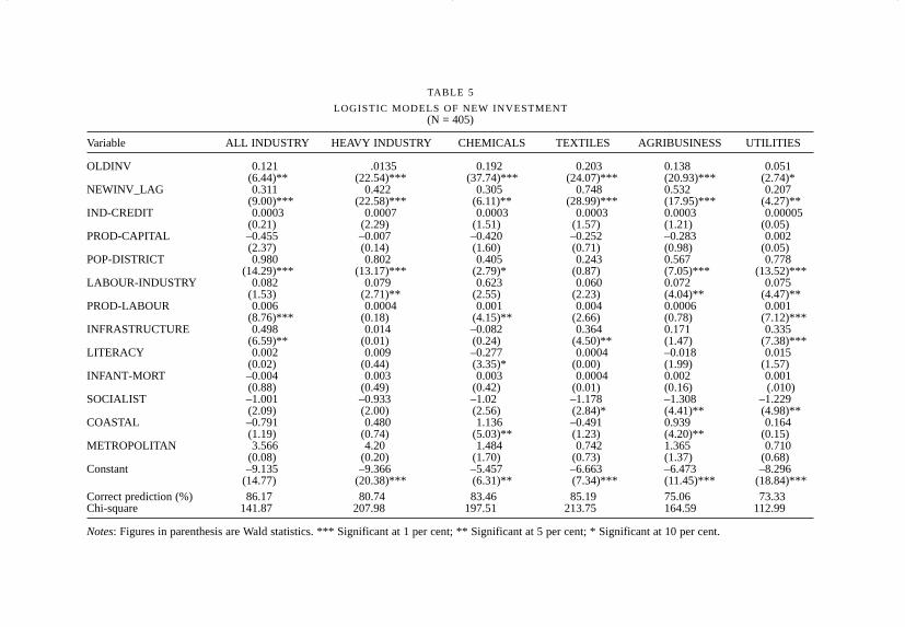
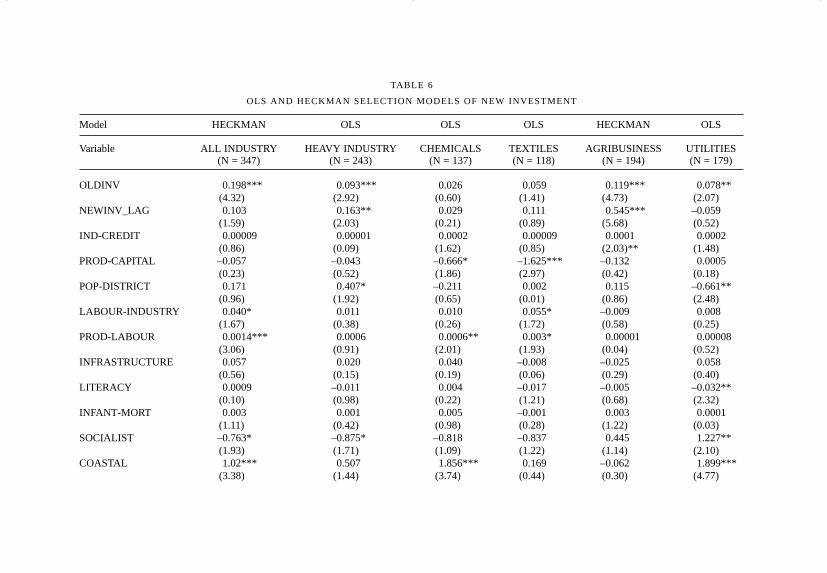
The logistic model results are reported in Table 5 and the OLS/Heckmanselection model results are reported in Table 6. Recall that the logistic modelsare to be used to identify the factors that contribute to a district getting some(as opposed to no) investment, and the OLS/Heckman selection models areto be used to identify the factors that contribute to the quantity of newinvestments. In the following discussion the results in the two tables areconsidered together and focused around the regressors or sets of independentvariables. But first consider the model sets as a whole. The logistic modelsare generally robust and predict over 73 per cent of the distribution ofdistricts with zero and non-zero investments. The OLS/ Heckman selectionmodels are robust, but generally less successful in explaining the variation inthe distribution of new investments. The adjusted R-square values go from alow of 0.112 for agribusiness to a high of 0.252 for all industry.

It is possible to improve the R-square values by adding variables whichare known to be influential: for instance, adding dummy regional or statevariables should show the attractiveness of the western region relative to theeastern region; the addition of a second spatial lag term, this time for theclustering effects of existing (or pre-reform) investment, is also likely toimprove the model fit. But these adjustments would not add to ourunderstanding of the investment distribution process. There is surely asubstantial random element in the distribution, but equally likely there arenon-random local factors that have not been modeled here, and that mayindeed be difficult to model. These factors relate to local or state levelpolicy changes (such as tax incentives, the location of export processingand/or free trade zones and so on), and some intangibles like culture,entrepreneurship and initiative.10 This is an important point and will beraised again later.

The concentration variable – old investment (OLDINV) – is consistentlysignificant in all logistic models, and in all but Chemicals and Textiles


402jds06.qxd 20/11/2003 10:06 Page 141

142T

HE

JOU

RN

AL

OF

DE

VE

LO

PM

EN

T S

TU

DIE

S

TABLE 5

LOGISTIC MODELS OF NEW INVESTMENT (N = 405)

Variable ALL INDUSTRY HEAVY INDUSTRY CHEMICALS TEXTILES AGRIBUSINESS UTILITIES

OLDINV 0.121 .0135 0.192 0.203 0.138 0.051(6.44)** (22.54)*** (37.74)*** (24.07)*** (20.93)*** (2.74)*

NEWINV_LAG 0.311 0.422 0.305 0.748 0.532 0.207(9.00)*** (22.58)*** (6.11)** (28.99)*** (17.95)*** (4.27)**

IND-CREDIT 0.0003 0.0007 0.0003 0.0003 0.0003 0.00005(0.21) (2.29) (1.51) (1.57) (1.21) (0.05)

PROD-CAPITAL –0.455 –0.007 –0.420 –0.252 –0.283 0.002(2.37) (0.14) (1.60) (0.71) (0.98) (0.05)

POP-DISTRICT 0.980 0.802 0.405 0.243 0.567 0.778(14.29)*** (13.17)*** (2.79)* (0.87) (7.05)*** (13.52)***

LABOUR-INDUSTRY 0.082 0.079 0.623 0.060 0.072 0.075(1.53) (2.71)** (2.55) (2.23) (4.04)** (4.47)**

PROD-LABOUR 0.006 0.0004 0.001 0.004 0.0006 0.001(8.76)*** (0.18) (4.15)** (2.66) (0.78) (7.12)***

INFRASTRUCTURE 0.498 0.014 –0.082 0.364 0.171 0.335(6.59)** (0.01) (0.24) (4.50)** (1.47) (7.38)***

LITERACY 0.002 0.009 –0.277 0.0004 –0.018 0.015(0.02) (0.44) (3.35)* (0.00) (1.99) (1.57)

INFANT-MORT –0.004 0.003 0.003 0.0004 0.002 0.001(0.88) (0.49) (0.42) (0.01) (0.16) (.010)

SOCIALIST –1.001 –0.933 –1.02 –1.178 –1.308 –1.229(2.09) (2.00) (2.56) (2.84)* (4.41)** (4.98)**

COASTAL –0.791 0.480 1.136 –0.491 0.939 0.164(1.19) (0.74) (5.03)** (1.23) (4.20)** (0.15)

METROPOLITAN 3.566 4.20 1.484 0.742 1.365 0.710(0.08) (0.20) (1.70) (0.73) (1.37) (0.68)

Constant –9.135 –9.366 –5.457 –6.663 –6.473 –8.296(14.77) (20.38)*** (6.31)** (7.34)*** (11.45)*** (18.84)***

Correct prediction (%) 86.17 80.74 83.46 85.19 75.06 73.33Chi-square 141.87 207.98 197.51 213.75 164.59 112.99

Notes: Figures in parenthesis are Wald statistics. *** Significant at 1 per cent; ** Significant at 5 per cent; * Significant at 10 per cent.

402jds06.qxd 20/11/2003 10:06 Page 142

143IN

DU

ST

RIA

L L

OC

AT

ION

IN P

OS

T-R

EF

OR

M IN

DIA

TABLE 6

OLS AND HECKMAN SELECTION MODELS OF NEW INVESTMENT

Model HECKMAN OLS OLS OLS HECKMAN OLS

Variable ALL INDUSTRY HEAVY INDUSTRY CHEMICALS TEXTILES AGRIBUSINESS UTILITIES(N = 347) (N = 243) (N = 137) (N = 118) (N = 194) (N = 179)

OLDINV 0.198*** 0.093*** 0.026 0.059 0.119*** 0.078**(4.32) (2.92) (0.60) (1.41) (4.73) (2.07)

NEWINV_LAG 0.103 0.163** 0.029 0.111 0.545*** –0.059(1.59) (2.03) (0.21) (0.89) (5.68) (0.52)

IND-CREDIT 0.00009 0.00001 0.0002 0.00009 0.0001 0.0002(0.86) (0.09) (1.62) (0.85) (2.03)** (1.48)

PROD-CAPITAL –0.057 –0.043 –0.666* –1.625*** –0.132 0.0005(0.23) (0.52) (1.86) (2.97) (0.42) (0.18)

POP-DISTRICT 0.171 0.407* –0.211 0.002 0.115 –0.661**(0.96) (1.92) (0.65) (0.01) (0.86) (2.48)

LABOUR-INDUSTRY 0.040* 0.011 0.010 0.055* –0.009 0.008(1.67) (0.38) (0.26) (1.72) (0.58) (0.25)

PROD-LABOUR 0.0014*** 0.0006 0.0006** 0.003* 0.00001 0.00008(3.06) (0.91) (2.01) (1.93) (0.04) (0.52)

INFRASTRUCTURE 0.057 0.020 0.040 –0.008 –0.025 0.058(0.56) (0.15) (0.19) (0.06) (0.29) (0.40)

LITERACY 0.0009 –0.011 0.004 –0.017 –0.005 –0.032**(0.10) (0.98) (0.22) (1.21) (0.68) (2.32)

INFANT-MORT 0.003 0.001 0.005 –0.001 0.003 0.0001(1.11) (0.42) (0.98) (0.28) (1.22) (0.03)

SOCIALIST –0.763* –0.875* –0.818 –0.837 0.445 1.227**(1.93) (1.71) (1.09) (1.22) (1.14) (2.10)

COASTAL 1.02*** 0.507 1.856*** 0.169 –0.062 1.899***(3.38) (1.44) (3.74) (0.44) (0.30) (4.77)

402jds06.qxd 20/11/2003 10:06 Page 143

144T

HE

JOU

RN

AL

OF

DE

VE

LO

PM

EN

T S

TU

DIE

S

METROPOLITAN 0.510 0.508 –0.305 0.339 0.021 0.971(1.01) (0.92) (.046) (0.65) (0.06) (1.53)

Constant 0.286 0.903 4.978* 4.384** –0.467 11.013***(0.18) (0.51) (1.78) (2.10) (0.37) (4.66)

Model Wald chi-sq 111.03*** 35.54*** 25.38** 31.19*** 63.77*** 43.07*** (Heckman Model)

Heckman Model lambda 0.674* 0.287 –0.358 –0.039 1.09*** 0.271(std. err. in parenthesis) (0.349) (0.437) (0.886) (0.746) (0.186) (0.867)

Adjusted R-Sq. from 0.252 0.134 0.157 0.146 0.112 0.151OLS model

Notes: *** Significant at 1 per cent; ** Significant at 5 per cent; * Significant at 10 per cent.

Figures in parenthesis are Z scores for the Heckman models, t statistics for the OLS models.

The Adjusted R-sq’s reported for the Heckman selection models are from the OLS models with the same functional forms. These are for informationonly. Likewise, the Wald and lambda reported for the OLS models are from the Heckman selection models with the same functional forms. Asdiscussed in the text, the Heckman selection model data for these instances (Heavy Industry, Chemicals, Textiles, and Utilities) are not shown becausethe lambdas are not significant, indicating that there is no selection bias in the OLS models.

TABLE 6 (Cont’d)

Model HECKMAN OLS OLS OLS HECKMAN OLS

Variable ALL INDUSTRY HEAVY INDUSTRY CHEMICALS TEXTILES AGRIBUSINESS UTILITIES(N = 347) (N = 243) (N = 137) (N = 118) (N = 194) (N = 179)

402jds06.qxd 20/11/2003 10:06 Page 144

among the OLS / Heckman selection models. The clustering variable – newinvestment in neighbouring districts (NEWINV-LAG) – is also verystrongly significant in all the logistic models, but not significant for allindustry, Chemicals, Textiles, or Utilities in the OLS / Heckman selectionmodel set. The parameter estimates for NEWINV-LAG are higher,indicating that the quantity of new neighboring investment has a strongerinfluence on the existence and quantity of new investment in a district.Generally, we can conclude that the concentration/clustering process,expressed through existing and new nearby investments, is very importantin determining whether or not a district gets any new investment, and isimportant, but less so, in determining the quantity of the new investment.

The capital variables – availability of industrial credit and theproductivity of capital – have virtually no influence on the location andquantity of new industrial investments. In fact, the capital-productivityvariable has a negative sign consistently through both model sets (with theexception of the Utilities sector), and in the OLS Chemicals and Textilesmodels, it is also significant. In other words, districts where theoutput–capital ratio is high the tendency is toward little or no newinvestment, and that this trend is particularly true of the Chemicals andTextiles sectors. The implication is that districts with low output–capitalratios (that is, districts with capital intensive investments) are preferred.This is not puzzling as much as it is an indirect confirmation of thecumulative causation thesis which suggests that capital-intensity will tendto favour geographical clustering of industry.

Of the Labour variables, the variable with consistent significance isdistrict population (POP-DISTRICT), which plays a positive role inattracting new industry (for all sectors except Textiles), but has littleinfluence in determining the quantity of new investment (a small positiveeffect is noted for Heavy Industry, and, not surprisingly, a negative effect isseen for Utilities). The size of the available industrial labour force has somesignificance, but only in the logistic models. Labour productivity (PROD-LABOUR) is inconsistently significant – primarily for all industry and theChemicals sector, and to a lesser extent the Utilities sector – where it has apositive role in both attracting new investment and on the quantity of newinvestment. Following the discussion in the preceding paragraph, thisimplies that capital-intensity of existing industry often plays a key role inattracting new investment.

The infrastructure variables have little overall significance indetermining the location or quantity of new industrial investment. Physicalinfrastructure (PHYS-INFRA, which is an index of access to nationalhighways, ports, and airports), appears to have some significance in the allindustry, Textiles, and Utilities logistic models, but none in any of the OLS


402jds06.qxd 20/11/2003 10:06 Page 145

/Heckman selection models. This is a somewhat unexpected finding.Perhaps this finding is an artifact of the way the PHYS-INFRA index hasbeen constructed. That, however, is unlikely, as this index was chosen afteran extensive sensitivity analysis among a large number of indexes,including the option of using the three infrastructure elementsindependently. This finding is consequential because, in policy circles,physical infrastructure is considered the key to attracting new investments(see the much discussed India Infrastructure Report, Expert Group, 1996).Yet, the models indicate that infrastructure does not play a role that isindependent of clustering processes. In other words, the establishment ofnew physical infrastructure is by itself unlikely to generate new industrialinvestments, especially in lagging regions.11

The social infrastructure variables (literacy and infant mortality), notsurprisingly, play no role in the new investment location decision. Literacy,when significant (or otherwise) is negatively related, and infant mortalityis unrelated. One can understand, even if one cannot endorse, theunexpected literacy effect. Statistically, it is probably the effect of Kerala’scombination of high literacy and low or no investment. But why shouldinfant mortality have no effect? After all there is great variation in thelevels of infant mortality, which averages around 60 in the south, rising to100 in Rajasthan, 120 in Uttar Pradesh, and 150 plus in Madhya Pradeshand Orissa. One can hope that this is a statistical artifact and not anindication of a social reality where new investments seek locations withhigh infant mortality.

At the same time, the Socialist variable (a proxy for unionised labour, orthe militancy of unionised labour)12 is negatively related to both theexistence and quantity of new investment. Perhaps the models are hinting atsome story about the quality of labour that new investment seeks. Industriallabour presence is favoured, but not if it is strongly unionised; the labourneed not be literate, in fact, literacy may work against attracting certainkinds of investment; and given that high infant mortality is indicative ofpoor social conditions and social infrastructure, the social conditions oflabour need not be progressive. The evidence presented here iscircumstantial – indeed, these models were not designed to examine therelationship between labour conditions and new investment – yet the trendsare troubling.

Of the two spatial dummy variables, the METROPOLITAN dummy hasno significance in any of the models, whereas the COASTAL dummy isweakly significant in some of the logistic models, and strongly significantin the OLS/Heckman selection models for all industry, Chemicals, andUtilities. The coastal bias of new investments (despite the absence ofinvestments in Kerala) has already been noted in the maps and tables;


402jds06.qxd 20/11/2003 10:06 Page 146

similarly, the finding on metropolises is unsurprising given that we havealready noted the relative decline of metropolitan districts.

CONCLUSIONS: CONCENTRATED DECENTRALISATION

It is clear that both in determining which districts get some new investmentand in determining the quantity of new investment, the most significantfactors are the existence and size of investment from the pre-reform periodand the existence and size of new investment in the neighbouring districts.The first factor implies continuity – evidence of a historical process ofinvestment location. The second factor implies clustering – evidence of therole of geography in guiding investment location. Both factors are strongerin determining success/failure rather than quantity. One implication of thisis that though historical processes are being continued in the choice ofinvestment location, the volume of new investments is following a differentpattern from the past. In other words, districts that were successful earliercontinue to receive new investment, but degree of past success is not thebest indicator of the degree of current success. The most successful pre-reform districts are not the most successful post-reform districts. There hasbeen a shift in geographical focus whereby new investments seek locationswithin the existing leading regions (or clusters), but at new locations withinthese regions. To use a concrete example highlighted earlier: GreaterBombay is still successful in attracting investment, but not to the extent itwas earlier; its neighbours, Raigarh and Thane, are now the preferredinvestment destinations.

Can the Indian experience on industrial location be placed in the contextof other developing nation experiences? There is evidence from SouthKorea [World Bank, 1999; Henderson, 1988; Lee, 1987] that as a result ofliberalisation in 1980s, the reinstatement of local government autonomy,and heavy communication infrastructure investments by the state awayfrom Seoul and Pusan, manufacturing industry has decentralised. Amongother physically small countries, there is a clear trend toward regionaldeconcentration of income and industry in Colombia; see Câ.rdenas andPontön [1995] on regional convergence and Lee [1987, 1989] on thedeconcentration of employment at the metropolitan level. In Indonesia, alarger country, the summary data suggest that some industrialdeconcentration has taken place during the reform period (the early 1980sonwards) in the secondary and tertiary sectors of the economy, whilegovernment consumption expenditure and fixed capital formation havebecome more concentrated [Akita and Lukman, 1995]; others note that‘these aggregate groupings … conceal important trends at the sub-regionallevel … There has almost certainly been a rising concentration of industrial


402jds06.qxd 20/11/2003 10:06 Page 147

activity on the fringes of major urban concentrations, such as Jakarta andSurabaya’ [Aswicahyono, Bird and Hill, 1996: 356; also Henderson andKuncoro, 1996]. Among countries that may be considered geographicallycomparable to India, the industrial location experience of Brazil has beenwidely studied. Townroe and Keen [1984] and Diniz [1994] have arguedthat ‘polarisation reversal’ has taken place in the state of São Paulo inBrazil, where an ‘agglomerative field’ with a radius of around 150kilometres around São Paulo is seeing faster industrial growth than the cityitself.13 According to Diniz, however, interregional industrial polarisationinto the South-east and the state of São Paulo continues.

Similarly, it appears that what is happening in India is quite distinct from‘spread’ or ‘polarisation reversal’ in that there is increasing inter-regionalpolarisation of industry at the same time that there is intraregional dispersalin the leading regions. In other words, the situation is one of concentrationwith dispersal, or to make an ironic use of the term, ‘concentrateddecentralisation’, where the new growth centres are in the advanced regionrather than in the periphery.14 Though the reforms of 1991 were used as thepoint of departure in the analysis, it does not follow that this concentrateddecentralisation process is purely the result of the reforms.

First, according to some scholars, the reforms began with Rajiv Gandhiin 1985; second, it is quite likely that some elements of the process,especially that of metropolitan decline, were well under way before anysuch formal, sharp transition (in 1985 or 1991). This raises the point thatthis study is unable to discern whether the changes are driven by changes intransport costs, agglomeration economies, or political action. I suggest thatthis is an issue of secondary importance, that is, relevant only at theintraregional scale. Remember that large parts of the country are marked bywhat has been termed ‘intangibles’ earlier in the article: Gujarat’sentrepreneurial culture, virtual stateless-ness in Bihar, extreme labourmilitancy in West Bengal, knowledge-based cultures in the south and so on.It is possible that these elements of local political economy create theprimary foundation on which interregional outcomes turn; that is, theindustrial location decision is a two-step process. First, there is the decisionon which general region to invest in, followed by the decision on thespecific location within the selected region. The first decision leads to inter-regional divergence; the second decision may lead to intra-regionalconvergence (due to declining transport costs and/or rising agglomerationdiseconomies). In India, the key is to device strategies that will influence thefirst decision.

final revision accepted November 2002


402jds06.qxd 20/11/2003 10:06 Page 148

NOTES

1. Geographers have been interested in this phenomenon for some time. However, their workis curiously marginalised in mainstream economics and development economics – perhapsdue to the different methodologies and epistemologies of the fields [Clark, 1998], perhapsdue to the analytical intractability of spatial parameters. As early as in the 1930s, Germangeographers theorised urban systems in terms of central place functions [Christaller, 1966]and systems of market areas [Losch, 1954], using concepts like ‘range of a good’ (atransport-cost factor) and ‘threshold population’ in a hierarchical diffusion structure.

2. The share of total investment allocated to each sector is somewhat consistent. Gains havebeen made in the Heavy Industries sector, where the pre- and post-reform shares wererespectively 33.4 and 37.2 per cent, and in the Chemicals and Petroleum sector, where theshares are 18.4 and 26.2 per cent; Losses have been in the Utilities sector with pre- and post-reform shares of 30.3 and 25.2 per cent, in Textiles with 7.8 and 5.7 per cent, and inAgribusiness with 7.1 and 2.9 per cent. I will suggest later that the CMIE Agribusiness dataare unreliable.

3. The maps show investment shares rather than per capita investment. There is little to choosebetween the two display methods. The latter method tends to de-emphasise the intensity ofinvestment in the more heavily populated metropolitan regions; that is, a map of thedistribution of shares tends to show more metropolitan and urban bias, but is also likely toprovide a better sense of industry concentration. Moreover, as all the other data are reportedin share rather than per capita terms, I have elected to present maps of investment shares. Theper capita maps are available with the author.

4. These data do not include figures for Jammu and Kashmir and the far north-eastern states(Arunachal Pradesh, Manipur, Meghalay, Mizoram, Nagaland, and Sikkim). Given theturmoil in Jammu and Kashmir, its data are unlikely to be reliable. In addition, all these statestogether accounted for less than 0.4 per cent of the total new industrial investment, almostentirely in utilities projects (typically hydel power), typically spread over several districts.Also note that the maps show data at the district level, but in order to minimise visual clutter,the district boundaries have not been drawn.

5. It is necessary to note that the government of Maharashtra takes this issue seriously enoughto dispute CMIE’s data. It feels that it remains the number one investment destination of thepost-reform period, and has considered legal action to dispute these figures. (Personalcommunication from CMIE officials.)

6. The disparity in Madhya Pradesh between the maps and the actual investment figures is aresult of the fact that investment is not evenly distributed within the state.

7. Andhra Pradesh is a bit of an anomaly. In popular accounts, the state led by dynamic ChiefMinister Chandrababu Naidu, is one of the prime beneficiaries of liberalisation (though inthe same popular accounts, questions are now being raised about the early fulsomeassessments.) The data here indicate that absent investments in the software sector (which iswhere AP has done well, and which are not included here), the state has lost its share ofindustry.

8. This may indicate that the post-reform or CMIE data for the Agribusiness sector areincomplete. In the pre-reform period, the Agribusiness sector had the highest level ofclustering. It is difficult to imagine a scenario whereby this extremely clustered industrywould suddenly lose the circumstances which enabled clustering in the first place, unless, asexpected, there are missing data. Remember the caution about missing small projects in theCMIE data. Since the Agribusiness sector is most likely to be composed of small factories(in the ASI data, this sector includes about 23 per cent of all factories but only about eightper cent of invested capital and five per cent of fixed capital), it is likely that the CMIE dataare incomplete for this sector. Henceforth, the results for the Agribusiness sector should beconsidered suspect.

9. For instance, the Kolkata metropolitan area includes the districts of Calcutta, Haora, Hugli,North 24 Parganas, and South 24 Parganas. Ahmedabad is the only city for which noadditional (sub-urban) district has been added.

10. For instance, one of the reasons popularly discussed for Gujarat’s success is the


402jds06.qxd 20/11/2003 10:06 Page 149

entrepreneurial culture of the local population which was supposedly kept under check in theprevious regime of licences and controls. This kind of thesis is probably best tested usingother methodologies (such as interview based detailed case studies), for it is difficult tocreate an objective index of entrepreneurial culture.

11. Does the inclusion of Physical Infrastructure as an explanatory variable introduce a problemof endogeneity? In other words, are both Physical Infrastructure and new investmentendogenously determined in a larger system (represented by the rest of the explanatoryfactors identified here), and is there a reciprocal causal connection between the twovariables? Had the two data series been taken from the same time period, that is, had PhysicalInfrastructure been represented by new investments in roads, ports, and so on, the problemof endogeneity would have been a serious one. However, as used here, the PhysicalInfrastructure data are historic, indexing a cumulation of infrastructure access indicators thatpredate the new investment data. There may indeed be a circular and cumulative relationshipbetween the two variables (in fact, this relationship is theorised at the outset), but as analysedhere there is no simultaneous relationship, nor are the determining factors the same.

12. West Bengal accounted for about 38 per cent and Kerala for over five per cent of theworkdays lost nation-wide in dispute-related stoppages between 1985 and 1995 (calculatedfrom Government of India [1997]).

13. The idea of ‘polarisation reversal’ followed from Hirschman’s notion of polariseddevelopment. This theory has been investigated by Richardson [1980] and Chakravorty[1994]. The latter has noted that the meaning of polarisation reversal depends on thedefinition of ‘pole’. He argues that declines in inter-urban, intra-metropolitan, and intra-regional concentration are all possible and likely in most developing nations, butinterregional inequality and concentration are likely to endure in large countries.

14. The term ‘concentrated decentralisation’ has been used in the growth pole literature, whereit meant that rather than scatter scarce investment resources around equally, ‘small centers orcores are set up in the periphery, thus to some extent distributing investment but also takingsome advantage of urbanisation economies’ [Darwent, 1975: 553]. For about two decades(the 1960s and 1970s) the growth pole policy was considered a critical tool that could helprealise agglomeration efficiencies while advancing the cause of inter-regional equity, makingit one of the most discussed ideas in urban and regional development [Hansen, 1967; Lo andSalih, 1981].

REFERENCES

Agresti, A., 1996, An Introduction to Categorical Data Analysis, New York: John Wiley.Ahluwalia, I.J., 1991, Productivity and Growth in Indian Manufacturing, Delhi: Oxford

University Press.Akita, T. and R.A. Lukman 1995, ‘Interregional Inequalities in Indonesia: A Sectoral Decomposition

Analysis for 1975-92’, Bulletin of Indonesian Economic Studies, Vol.31, No.2, 61–81.Alonso, W., 1980, ‘Five Bell Shapes in Development’, Papers of the Regional Science

Association, Vol.45, 1, pp.5–16.Amemiya, T., 1985, Advanced Econometrics, Oxford: Basil Blackwell.Anselin, L., 1992, Spacestat Manual, Morgantown, VA: University of West Virginia.Aswicahyono, H.H., Bird, K. and H. Hill, 1996, ‘What Happens to Industrial Structure When

Countries Liberalize? Indonesia Since the Mid-1980’s’, The Journal of Development Studies,Vol.32, No.3, pp.340–63.

Awasthi, D.N., 1991, Regional Patterns of Industrial Growth in India, New Delhi: ConceptPublishing.

Becker, C.M., Williamson, J.G. and E.S. Mills, 1992, Indian Urbanization and Economic Growthsince 1960, Baltimore, MD: Johns Hopkins University Press.

Byres, T.J. (ed.), 1997, The State, Development Planning and Liberalisation in India, Delhi:Oxford University Press.

Câ.rdenas, M. and A. Pontön, 1995, ‘Growth and Convergence in Colombia: 1950–1990’,Journal of Development Economics, Vol.47, No.1, pp.5–37.


402jds06.qxd 20/11/2003 10:06 Page 150

Chakravorty, S., 1994, ‘Equity and the Big City’, Economic Geography, Vol.70, No.1, pp.1–22.Chakravorty, S., 2000, ‘How Does Structural Reform Affect Regional Development? Resolving

Contradictory Theory with Evidence from India’, Economic Geography, Vol.76, No.4,pp.367–94.

Chapman, K. and D.F. Walker, 1991, Industrial Location: Principles and Policies, Oxford: BasilBlackwell.

Christaller, W., 1966, Central Places in Southern Germany (trans. by C.W. Baskin), EnglewoodCliffs, NJ: Prentice Hall (original published in 1933).

Clark, G.L., 1998, ‘Stylized Facts and Close Dialogue: Methodology in Economic Geography’,Annals of the Association of American Geographers, Vol.88, No.1, pp.73–87.

CMIE (Centre for Monitoring Indian Economy), 1993, Profiles of Districts, Mumbai: Centre forMonitoring Indian Economy.

Das, S.K. and A. Barua, 1996, ‘Regional Inequalities, Economic Growth and Liberalisation: AStudy of the Indian Economy’, The Journal of Development Studies, Vol.32, No.3,pp.364–90.

Darwent, D.F., 1975, ‘Growth Poles and Growth Centers in Regional Planning: A Review’,Friedmann and Alonso (eds.), in Regional Policy: Readings in Theory and ApplicationsCambridge, MA: MIT Press.

Dehejia, J., 1993, ‘Economic Reforms: Birth of an “Asian Tiger”’, in P. Oldnburg (ed.), IndiaBriefing, Boulder, CO: Westview.

Diniz, C.C., 1994, ‘Polygonized Development in Brazil: Neither Decentralization nor ContinuedPolarization’, International Journal of Urban and Regional Research, Vol.18, No.2,pp.293–314.

Elizondo, R.L. and P. Krugman, 1992, Trade Policy and the Third World Metropolis, NBERWorking Paper No.4238, Cambridge, MA: NBER.

Ellison, G. and E.L. Glaeser, 1997, ‘Geographic Concentration in U.S. Manufacturing Industries:A Dartboard Approach’, Journal of Political Economy, Vol.105, No.5, pp.889–927.

Expert Group (on the Commercialisation of Infrastructure Projects), 1996, The IndiaInfrastructure Report: Policy Imperatives for Growth and Welfare, New Delhi: NationalCouncil of Applied Economic Research.

Friedmann, J., 1973, ‘A Theory of Polarized Development’, in J. Friedmann (ed.), Urbanization,Planning and National Development, Beverly Hills, CA: Sage, pp.41–64.

Fujita, M., Krugman, P. and A.J. Venables, 1999, The Spatial Economy: Cities, Regions, andInternational Trade, Cambridge, MA: The MIT Press.

Gilbert, A., 1993, ‘Third World Cities: The Changing National Settlement System’, UrbanStudies, Vol.30, Nos.4,5, pp.721–40.

Goldar, B., 1997, ‘Econometrics of Indian Industry’, in K.L. Krishna (ed.), EconometricApplications in India, New Delhi: Oxford University Press.

Government of India, 1997, Handbook of Industrial Policy and Statistics 1997, New Delhi:Ministry of Industry.

Hansen, N.M., 1967, ‘Development Pole Theory in a Regional Context’, Kyklos, Vol.20, No.3,pp.709–27.

Harrington, J.W. and B. Warf, 1995, Industrial Location: Principles, Practice, and Policy,London and New York: Routledge.

Henderson, J.V., 1988, Urban Development: Theory, Fact, and Illusion, New York: OxfordUniversity Press.

Henderson, J.V. and A. Kuncoro, 1996, ‘Industrial Centralization in Indonesia’, World BankEconomic Review, Vol.10, No.3, pp.513–40.

Hirschman, A.O., 1958, The Strategy of Economic Development, New Haven, CT: YaleUniversity Press.

Hoover, E.M., 1968, The Location of Economic Activity, New York: McGraw Hill.Joshi, V. and I.M.D. Little, 1997, India’s Economic Reforms 1991–2001, Delhi: Oxford

University Press.Krugman, P., 1991, Geography and Trade, Cambridge, MA: MIT Press.Krugman, P., 1996, ‘Urban Concentration: The Role of Increasing Returns and Transport Costs’,

International Regional Science Review, Vol.19, Nos.1,2, pp.5–30.


402jds06.qxd 20/11/2003 10:06 Page 151

Lee, K.S., 1987, ‘Employment Location and Spatial Policies: Colombia and Korea’, in G.S.Tolley and V. Thomas (eds.), The Economics of Urbanization and Urban Policies inDeveloping Countries, Washington, DC: The World Bank, pp.94–105.

Lee, K.S., 1989, The Location of Jobs in a Developing Metropolis: Patterns of Growth in Bogotáand Cali, Colombia, NY: Oxford University Press for the World Bank.

Lo, F.C. and K. Salih, 1981, ‘Growth Poles, Agropolitan Development and Polarization Reversal:The Debate and Search for Alternatives’, in Stohr and Taylor (eds.), Development FromAbove or Below? The Dialectics of Regional Planning in Developing Countries, Chichester:John Wiley & Sons.

Losch, A., 1954, The Economics of Location (trans. by W.H. Woglom and W.F. Stolper), NewHaven, CT: Yale University Press (original published in 1938).

Myrdal, G., 1957, Economic Theory and Underdeveloped Regions, London: Duckworth.National Commission on Urbanization, 1988, Report, New Delhi: Government of India.Perroux, F., 1950, ‘Economic Space: Theory and Applications’, Quarterly Journal of Economics,

Vol.64, No.1, pp.89–104.Rajan, S.I. and P. Mohanchandran, 1998, ‘Infant and Child Mortality Estimates – Part I’,

Economic and Political Weekly, Special Statistics, 9 May, Vol.34, No.19, pp.1120–40.Richardson, H.W., 1973, Regional Growth Theory, London: Macmillan.Richardson, H.W., 1980, ‘Polarization Reversal in Developing Countries’, Papers of the

Regional Science Association, Vol.45, No.1, pp.67–85.Rosenthal, S.S. and W.C. Strange, 2001, ‘The Determinants of Agglomeration’, Journal of Urban

Economics, Vol.50, No.2, pp.191–229.Saha, S.K., 1987, Industrialization and Development in Space: An Indian Perspective, Swansea:

Center for Development Studies.Sala-i-Martin, X., 1996, ‘Regional Cohesion: Evidence and Theories of Regional Growth and

Convergence’, European Economic Review, Vol.40, No.6, pp.1325–52.Shukla V., 1984, ‘The Productivity of Indian Cities and Some Implications for Development

Policy’, unpublished PhD, thesis, Princeton, NJ: Princeton University Press.Townroe, P.M and D. Keen, 1984, ‘Polarization Reversal in the State of São Paulo, Brazil’,

Regional Studies, Vol.18, No.1, pp.45–54.Vella, F., 1998, ‘Estimating Models with Sample Selection Bias: A Survey’, The Journal of

Human Resources, Vol.33, No.1, pp.127–69.Verma, S., 1986, ‘Urbanization and Productivity in Indian States’, in E.S. Mills and C.M. Becker

(eds.), Studies in Indian Urban Development, Washington, DC: World Bank, pp.103–36.White, M.J., 1983, ‘The Measurement of Spatial Segregation’, American Journal of Sociology,

Vol.88, No.5, pp.1008–19.Williamson, J., 2000, ‘What Should the World Bank Think About the Washington Consensus?’

World Bank Research Observer, Vol.15, No.2, pp.251–64.Williamson, J.G., 1965, ‘Regional Inequality and the Process of National Development’,

Economic Development and Cultural Change, Vol.13, No.2, pp.3–45.Winship, C. and R.D. Mare, 1992, ‘Models for Sample Selection Bias’, Annual Review of

Sociology, Vol.18, No.1, pp.327–50.World Bank, 1999, Entering the 21st Century: World Development Report 1999/2000,

Washington, DC: World Bank.


402jds06.qxd 20/11/2003 10:06 Page 152

industrial location in post-reform india: patterns of inter ...sanjoy/jds.pdfpatterns of...

Documents