industrial cfd simulation of aerodynamic … · decided to use the general purpose cfd software...
TRANSCRIPT

UNIVERSITÀ DEGLI STUDI DI NAPOLI FEDERICO II
DOTTORATO DI RICERCA IN INGEGNERIA AEROSPAZIALE,
NAVALE, E DELLA QUALITÀ (XXI CICLO)
DIPARTIMENTO DI INGEGNERIA AEROSPAZIALE
______________________________________
INDUSTRIAL CFD SIMULATION
OF AERODYNAMIC NOISE
______________________________________
Domenico Caridi
Il Coordinatore: Il Tutore:
Ch.mo Prof. Antonio Moccia Ch.mo Prof. Carlo De Nicola
A.A. 2007˗2008

i
ABSTRACT
INDUSTRIAL CFD SIMULATION
OF AERODYNAMIC NOISE
Domenico Caridi
DIPARTIMENTO DI INGEGNERIA AEROSPAZIALE
Real challenges to suppress undesirable fluid-excited acoustics are posed by a
wide variety of engineering disciplines. Noise regulations, passenger comfort and
component stability are motivators which are continuing to stimulate substantial efforts
towards the understanding of aeroacoustic phenomena, and not least to quantify the
usability (practicability and value) of traditional and advanced prediction methods. The
latter is the primary focus of this thesis, particularly as applied to the transportation
industries, aerospace, automotive and rail.
Nowadays Computational Fluid Dynamics (CFD) is a tool well integrated into the
industrial development and production life-cycles. This is possible now because of two
main factors: the increase in the performance of relatively cheap personal computers and
network facilities, and the progress made in general purpose CFD software between
modeling complexity and practicability within the industrial environment.

ii
While CFD methodologies are well established for lots of applications such as
aerodynamics, heat exchange, etc., aeroacoustic CFD simulations still represent a
challenge, in particular their industrial practicability. In these years this has given rise to
heavy investments by the automotive industry in international aeroacoustics consortia,
whereby all the major car companies work together to study the limitations and
advantages of aeroacoustics CFD. The general aim of these consortia is to develop
methodologies which fit into, and improve upon, current design processes.
The goal of the present work is to explore the multitude of different CFD
modeling approaches for some typical industrial problems such as: cavity noise, vortex
shedding noise, propeller and jet noise. Each of these problems has a particular
mechanism for noise generation and different methods have been studied and tested, in
order to develop and optimize a practical methodology for the analysis of each problem
type. Furthermore each of the aeroacoustics problems considered are representative of a
variety of industrial applications. Cavity noise is at the origin of phenomena such as sun-
roof buffeting in convertibles or door-gap tonal noise. Vortex shedding noise is typical
of any flows involving bluff bodies such as automobile antennas or aircraft landing gear.
Propeller noise is typical to applications involving rotating machinery, such as fans,
pumps and turbines.
Different approaches ranging from steady and transient RANS simulations with
the acoustic analogy (including porous and solid surface formulations), to Computational
Aero Acoustics (CAA) and Large Eddy Simulation (LES) type computations have been
studied and applied.
iii
Classic theories already exist to predict aerodynamically generated noise, which
are both computationally and economically less expensive than CFD methods. However
aeroacoustics CFD is the future, beginning as a promising present, for the following
reasons:
Industries are interested in modeling complex geometries.
Many classic theories can be applied successfully but very often
restrictions exist with respect to the configuration and flow conditions. For
example, classic propeller theories cannot be used to model real-world
configurations such as a propeller installed on a wing with some
prescribed yaw or angle of attack.
The progress of all other Computer Aided Design and Engineering tools,
such as linear or non-linear structural codes, are driving design towards a
virtual multi-physics approach for the simulation of complex geometries.
Due to previous experience and the wide availability of modeling options, it was
decided to use the general purpose CFD software package ANSYS FLUENT for CFD
investigations in this study.

iv
ACKNOWLEDGMENTS
First of all I wish to thank my advisor Prof. Carlo De Nicola for his support and
help in this path of human and professional growth. The coordinator Prof. Antonio
Moccia for his comprehension about some difficulties to conciliate my job with the PHD
activities. I would also like to thank Chris Carey and Dave Mann from ANSYS for their
support and attention to this PHD which was started prior to me joining the company. A
special thank also to Andy Wade from ANSYS for his valuable help and encouragement.
I am grateful to the PHD student Michele De Gennaro, Ing. Giovanni Petrone and the
student Gianpaolo Reina for their contribution to this work.

v
TABLE OF CONTENTS
1 ACOUSTICS FUNDAMENTALS .......................................................................... 1
1.1 PHYSICS OF SOUND ....................................................................................... 1
1.2 SOUND FIELD DEFINITIONS ........................................................................ 7
1.2.1 Free Field ........................................................................................................ 7
1.2.2 Near Field........................................................................................................ 7
1.2.3 Far Field .......................................................................................................... 7
1.2.4 Direct Field ..................................................................................................... 7
1.2.5 Reverberant Field............................................................................................ 8
1.2.6 Frequency Analysis......................................................................................... 8
1.2.6.1 A convenient property of the one-third octave band centre frequencies ...... 10
1.3 QUANTIFICATION OF SOUND.................................................................... 12
1.3.1 Sound Power (W) and Intensity (I) ............................................................... 12
1.3.2 Sound Pressure Level.................................................................................... 13
1.3.3 Sound Intensity Level ................................................................................... 15
1.3.4 Sound Power Level ....................................................................................... 15
1.3.5 Combining Sound Pressures ......................................................................... 16
vi
1.3.5.1 Addition of coherent sound pressures........................................................... 16
1.3.5.2 Addition of incoherent sound pressures (logarithmic addition) ................... 17
1.4 PROPAGATION OF NOISE ........................................................................... 20
1.4.1 Free Field ...................................................................................................... 20
1.4.2 Directivity ..................................................................................................... 22
1.4.3 Reflection effects .......................................................................................... 23
1.4.4 Reverberant fields ......................................................................................... 24
1.4.5 Types of Noise .............................................................................................. 26
2 AERODYNAMIC SOUND .................................................................................... 31
2.1 HOMOGENOUS WAVE PROPAGATION.................................................... 32
2.2 NON-HOMOGENEOUS WAVE PROPAGATION ....................................... 33
2.3 LIGHTHILL’S ANALOGY ............................................................................. 35
2.4 CURLE’S EQUATION .................................................................................... 36
2.5 THE FFOWCS WILLIAMS & HAWKINGS’S ANALOGY ......................... 40
2.6 CONSIDERATIONS ON THE SOUND GENERATED AERODYNAMICALLY.................................................................................. 46
2.7 FLUENT IMPLEMENTATION OF ACOUSTIC ANALOGY ...................... 49
3 AEROACOUSTICS SIMULATION APPROACHES........................................ 53
3.1 COMPUTATIONAL AEROACOUSTICS...................................................... 54
3.1.1 Range of Scales............................................................................................. 55
3.1.2 Range of Pressures ........................................................................................ 56
3.2 CFD-WAVE-EQUATION-SOLVER COUPLING ......................................... 57
3.3 INTEGRAL ACOUSTICS METHODS........................................................... 59
3.4 SYNTHETIC NOISE GENERATION METHOD........................................... 59
4 NOISE GENERATION MECHANISM ............................................................... 62
4.1 CAVITY NOISE............................................................................................... 62

vii
4.2 VORTEX SHEDDING NOISE ........................................................................ 66
4.3 AIRFOIL SELF-NOISE ................................................................................... 71
4.3.1 Turbulent-Boundary-Layer-Trailing-Edge (TBL-TE) Noise ....................... 73
4.3.2 Separation-Stall Noise .................................................................................. 74
4.3.3 Laminar-Boundary-Layer-Vortex-Shedding (LBL-VS) Noise .................... 74
4.3.4 Tip Vortex Formation Noise ......................................................................... 75
4.3.5 Noise Trailing-Edge-Bluntness Vortex-Shedding ........................................ 75
4.3.6 Airfoil Tonal Noise ....................................................................................... 76
4.4 PROPELLER NOISE ....................................................................................... 79
4.4.1 High Performance Propeller and Installation Noise ..................................... 79
4.4.2 Propeller Noise Characteristics..................................................................... 83
4.4.3 Steady Sources .............................................................................................. 85
4.4.4 Unsteady Sources.......................................................................................... 86
4.4.5 Random Sources ........................................................................................... 88
4.4.6 Non Linear Effects ........................................................................................ 89
4.5 JET NOISE ....................................................................................................... 92
4.5.1 Jet Noise Physics........................................................................................... 93
4.5.2 Heated Jet Noise – The Effects of Increased Temperature........................... 97
5 EXAMPLES OF AEROACOUSTICS SIMULATIONS .................................. 101
5.1 CAVITY NOISE............................................................................................. 101
5.1.1 Experiments ................................................................................................ 102
5.1.2 Simulation Set Up ....................................................................................... 104
5.1.3 Results......................................................................................................... 106
5.2 VORTEX SHEDDING NOISE ...................................................................... 111
5.2.1 Experiments ................................................................................................ 111

viii
5.2.2 Simulation Set Up ....................................................................................... 111
5.2.3 Results......................................................................................................... 116
5.3 PROPELLER NOISE ..................................................................................... 125
5.3.1 Experiments ................................................................................................ 125
5.3.1.1 NASA SR2.................................................................................................. 125
5.3.1.2 NACA 4-(3)(08)-03 .................................................................................... 130
5.3.2 Simulation Set Up ....................................................................................... 133
5.3.3 Results......................................................................................................... 141
5.3.3.1 NASA SR2.................................................................................................. 141
5.3.3.2 NACA 4-(3)(08)-03 .................................................................................... 146
5.4 JET NOISE ..................................................................................................... 153
5.4.1 Experiments ................................................................................................ 153
5.4.2 Simulation Set Up ....................................................................................... 158
5.4.3 Results......................................................................................................... 164
6 CONCLUSION ..................................................................................................... 171
References...................................................................................................................... 176

ix
NOMENCLATURE
c speed of sound [m/s]
Cd drag coefficient
d diameter [m]
G green function
k turbulence kinetic energy [m2/s2]
M Mach number
n surface normal vector
p pressure [Pa]
pref reference pressure [Pa]
P production of turbulent kinetic energy [kg/(m s2)]
R ideal gas constant [J/mol/K]
Re Reynolds number
St Strouhal number
t time [s]
T temperature [K] or [°C]
Tj jet core temperature [K] or [°C]
ijT Lighthill stress tensor components [N/m2]

x
Uj axial jet velocity [m/s]
ui velocity component in the i direction [m/s]
xi coordinate vector [m]
y+ normalized wall coordinate
blade angle at 75 % of blade radius [degree]
ij Kronecker delta tensor [dimensionless]
turbulence dissipation rate [m2/s3]
wavelength [m]
dynamic viscosity [kg/(m s)]
t dynamic turbulence viscosity [kg/(m s)]
kinematic viscosity [m2/s]
density [kg/m3]
retarded time [s]
ij stress tensor components [N/m2]
w wall shear stress [N/m2]
prime (‘ ) fluctuating quantity
overbar (¯) time averaged quantity

xi
ACRONYMS
2D Two Dimension
3D Three Dimension
BL Boundary Layer
CAA Computational Aero Acoustics
CFL Courant Number
CFD Computational Fluid Dynamics
DES Detached Eddy Simulation
DNS Direct Numerical Simulation
FFT Fast Fourier Transform
FW-H Ffowcs Williams and Hawkings
LBL Laminar Boundary Layer
LES Large Eddy Simulation
MRF Moving Reference Frame
MUSCL Monotone Upstream-Centered Schemes for Conservation Laws
OPSL Overall Sound Pressure Level
PBCS Pressure Based Coupled Solver
NRBC Non Reflective Boundary Condition

xii
PISO Pressure-Implicit with Splitting of Operators
PRESTO PREssure STaggering Option
QUICK Quadratic Upstream Interpolation for Convective Kinematics
RANS Reynolds-Averaged Navier-Stokes
RMS Root-Mean-Square
RSM Reynolds Stress Model
SIMPLE Semi-Implicit Pressure Linked Equations
SLM Sliding Mesh
SPL Sound Pressure Level
TBL Turbulent Boundary Layer
TE Trailing Edge
TI Turbulent Intensity [%]
TKE Turbulent Kinetic Energy [m2/s2]
UDF User-Defined Function
VS Vortex Shedding

1
1 ACOUSTICS FUNDAMENTALS
To provide the necessary background for the understanding of the topics covered
in this thesis, basic definitions and other aspects related to the physics of sound and noise
are presented. Most definitions have been internationally standardized and are listed in
standards publications such as IEC 60050-801(1994).
1.1 PHYSICS OF SOUND
Noise can be defined as "disagreeable or undesired sound" or other disturbance.
From the acoustics point of view, sound and noise constitute the same phenomenon of
atmospheric pressure fluctuations about the mean atmospheric pressure; the
differentiation is greatly subjective. What is sound to one person can very well be noise
to somebody else.
Sound (or noise) is the result of pressure variations, or oscillations, in an elastic
medium (e.g., air, water, solids), generated by a vibrating surface, or turbulent fluid flow.
Sound propagates in the form of longitudinal (as opposed to transverse) waves, involving
a succession of compressions and rarefactions in the elastic medium, as illustrated by
Figure 1-1(a). When a sound wave propagates in air (which is the medium considered in
this document), the oscillations in pressure are above and below the ambient atmospheric
pressure.

2
Figure 1-1 Representation of a sound wave. (a) compressions and rarefactions caused in air by the sound wave.(b) graphic representation of pressure variations above and below atmospheric pressure.
Figure 1-2 Wavelength in air versus frequency.

3
The speed of sound propagation, c, the frequency, f, and the wavelength, λ, are
related by the following equation:
fc
(1.1)
the speed of propagation, c, of sound in air is 343 m/s, at 20 C and 1 atmosphere
pressure. At other temperatures (not too different from 20 C), it may be calculated using:
Tcc 6.0332
(1.2)
where Tc is the temperature in C. Alternatively, making use of the equation of
state for gases, the speed of sound may be written as:
MRTc k
(1.3)
where Tk is the temperature in K, R is the universal gas constant which has the
value 8.314 J per mole K, and M is the molecular weight, which for air is 0.029 kg/mole.
For air, the ratio of specific heats, γ, is 1.402.
All of the properties just discussed (except the speed of sound) apply only to a
pure tone (single frequency) sound which is described by the oscillations in pressure
shown in Figure 1-1. However, sounds usually encountered are not pure tones. In general,
sounds are complex mixtures of pressure variations that vary with respect to phase,
frequency, and amplitude. For such complex sounds, there is no simple mathematical
relation between the different characteristics. However, any signal may be considered as
a combination of a certain number (possibly infinite) of sinusoidal waves, each of which
may be described as outlined above. These sinusoidal components constitute the
4
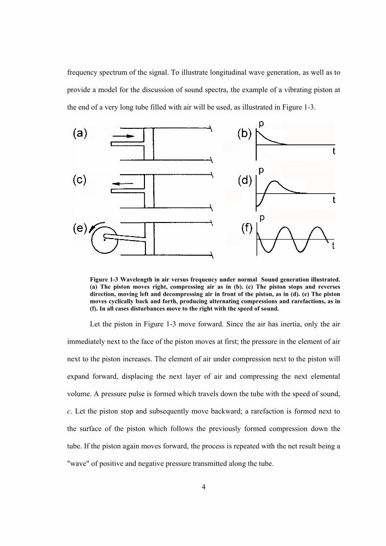
frequency spectrum of the signal. To illustrate longitudinal wave generation, as well as to
provide a model for the discussion of sound spectra, the example of a vibrating piston at
the end of a very long tube filled with air will be used, as illustrated in Figure 1-3.
Figure 1-3 Wavelength in air versus frequency under normal Sound generation illustrated. (a) The piston moves right, compressing air as in (b). (c) The piston stops and reverses direction, moving left and decompressing air in front of the piston, as in (d). (e) The piston moves cyclically back and forth, producing alternating compressions and rarefactions, as in (f). In all cases disturbances move to the right with the speed of sound.
Let the piston in Figure 1-3 move forward. Since the air has inertia, only the air
immediately next to the face of the piston moves at first; the pressure in the element of air
next to the piston increases. The element of air under compression next to the piston will
expand forward, displacing the next layer of air and compressing the next elemental
volume. A pressure pulse is formed which travels down the tube with the speed of sound,
c. Let the piston stop and subsequently move backward; a rarefaction is formed next to
the surface of the piston which follows the previously formed compression down the
tube. If the piston again moves forward, the process is repeated with the net result being a
"wave" of positive and negative pressure transmitted along the tube.

5
Figure 1-4 Spectral analysis illustrated. (a) Disturbance p varies sinusoidally with time t at a single frequency f1, as in (b). (c) Disturbance p varies cyclically with time t as a combination of three sinusoidal disturbances of fixed relative amplitudes and phases; the associated spectrum has three single-frequency components f1, f2 and f3, as in (d). (e) Disturbance p varies erratically with time t, with a frequency band spectrum as in (f).
If the piston moves with simple harmonic motion, a sine wave is produced; that is,
at any instant the pressure distribution along the tube will have the form of a sine wave,
or at any fixed point in the tube the pressure disturbance, displayed as a function of time,
will have a sine wave appearance. Such a disturbance is characterized by a single
frequency. The motion and corresponding spectrum are illustrated in Figure 1-4a and b.
If the piston moves irregularly but cyclically, for example, so that it produces the
waveform shown in Figure 1-4c, the resulting sound field will consist of a combination of
sinusoids of several frequencies. The spectral (or frequency) distribution of the energy in

6
this particular sound wave is represented by the frequency spectrum of Figure 1-4d. As
the motion is cyclic, the spectrum consists of a set of discrete frequencies.
Although some sound sources have single-frequency components, most sound
sources produce a very disordered and random waveform of pressure versus time, as
illustrated in Figure 1-4e. Such a wave has no periodic component, but by Fourier
analysis it can be shown that the resulting waveform may be represented as a collection
of waves of all frequencies. For a random type of wave the sound pressure squared in a
band of frequencies is plotted as shown in the frequency spectrum of Figure 1-4f.
It is customary to refer to spectral density level when the measurement band is
one Hz wide, to one third octave or octave band level when the measurement band is one
third octave or one octave wide and to spectrum level for measurement bands of other
widths.
Two special kinds of spectra are commonly referred to as white random noise and
pink random noise. White random noise contains equal energy per hertz and thus has a
constant spectral density level. Pink random noise contains equal energy per
measurement band and thus has an octave or one-third octave band level which is
constant with frequency.

7
1.2 SOUND FIELD DEFINITIONS
Following Sound Field Definitions. For more detail see ISO 12001.
1.2.1 Free Field
The free field is a region in space where sound may propagate free from any form
of obstruction.
1.2.2 Near Field
The near field of a source is the region close to a source where the sound pressure
and acoustic particle velocity are not in phase. In this region the sound field does not
decrease by 6 dB each time the distance from the source is doubled. The near field is
limited to a distance from the source equal to about a wavelength of sound or equal to
three times the largest dimension of the sound source (whichever is the larger).
1.2.3 Far Field
The far field of a source begins where the near field ends and extends to infinity.
Note that the transition from near to far field is gradual in the transition region. In the far
field, the direct field radiated by most machinery sources will decay at the rate of 6 dB
each time the distance from the source is doubled. For line sources such as traffic noise,
the decay rate varies between 3 and 4 dB.
1.2.4 Direct Field
The direct field of a sound source is defined as that part of the sound field which
has not suffered any reflection from any room surfaces or obstacles.

8
1.2.5 Reverberant Field
The reverberant field of a source is defined as that part of the sound field radiated
by a source which has experienced at least one reflection from a boundary of the room or
enclosure containing the source.
1.2.6 Frequency Analysis
Frequency analysis may be thought of as a process by which a time varying signal
in the time domain is transformed to its frequency components in the frequency domain.
It can be used for quantification of a noise problem, as both criteria and proposed controls
are frequency dependent. In particular, tonal components which are identified by the
analysis may be treated somewhat differently than broadband noise. Sometimes
frequency analysis is used for noise source identification and in all cases frequency
analysis will allow determination of the effectiveness of controls.
There are a number of instruments available for carrying out a frequency analysis
of arbitrarily time-varying signals . To facilitate comparison of measurements between
instruments, frequency analysis bands have been standardized. Thus the International
Standards Organization has agreed upon "preferred" frequency bands for sound
measurement and analysis.
The widest band used for frequency analysis is the octave band; that is, the upper
frequency limit of the band is approximately twice the lower limit. Each octave band is
described by its "centre frequency", which is the geometric mean of the upper and lower
frequency limits. The preferred octave bands are shown in the Table of Figure 1-5, in
terms of their centre frequencies. Occasionally, a little more information about the
detailed structure of the noise may be required than the octave band will provide. This

9
can be obtained by selecting narrower bands; for example, one-third octave bands. As the
name suggests, these are bands of frequency approximately one-third of the width of an
octave band. Preferred one-third octave bands of frequency have been agreed upon and
are also shown in the Table of Figure 1-5.
Instruments are available for other forms of band analysis. However, they do not
enjoy the advantage of standardization so that the inter-comparison of readings taken on
such instruments may be difficult. One way to ameliorate the problem is to present such
readings as mean levels per unit frequency. Data presented in this way are referred to as
“Spectral Density Levels” as opposed to band levels. In this case the measured level is
reduced by ten times the logarithm to the base ten of the bandwidth. For example,
referring to the Table of Figure 1-5, if the 500 Hz octave band which has a bandwidth of
354 Hz were presented in this way, the measured octave band level would be reduced by
10 log10 (354) = 25.5 dB to give an estimate of the spectral density level at 500 Hz.
The problem is not entirely alleviated, as the effective bandwidth will depend
upon the sharpness of the filter cut-off, which is also not standardized. Generally, the
bandwidth is taken as lying between the frequencies, on either side of the pass band, at
which the signal is down 3 dB from the signal at the centre of the band.
There are two ways of transforming a signal from the time domain to the
frequency domain. The first involves the use of band limited digital or analog filters. The
second involves the use of Fourier analysis where the time domain signal is transformed
using a Fourier series. This is implemented in practice digitally (referred to as the DFT -
digital Fourier Transform) using a very efficient algorithm known as the FFT (Fast
Fourier Transform).

10
1.2.6.1 A convenient property of the one-third octave band centre frequencies
The one-third octave band centre frequency numbers have been chosen so that
their logarithms are one-tenth decade numbers. The corresponding frequency pass bands
are a compromise; rather than follow a strictly octave sequence which would not repeat,
they are adjusted slightly so that they repeat on a logarithmic scale. For example, the
sequence 31.5, 40, 50 and 63 has the logarithms 1.5, 1.6, 1.7 and 1.8. The corresponding
frequency bands are sometimes referred to as the 15th, 16th, etc., frequency bands.

11
Figure 1-5 Frequency Band Table.

12
1.3 QUANTIFICATION OF SOUND
1.3.1 Sound Power (W) and Intensity (I)
The Sound intensity is a vector quantity determined as the product of sound
pressure and the component of particle velocity in the direction of the intensity vector. It
is a measure of the rate at which work is done on a conducting medium by an advancing
sound wave and thus the rate of power transmission through a surface normal to the
intensity vector. It is expressed as watts per square meter (W/m2). In a free-field
environment, i.e., no reflected sound waves and well away from any sound sources, the
sound intensity is related to the root mean square acoustic pressure as follows
2
c
pI rms
(1.4)
where ρ is the density of air (kg/m3), and c is the speed of sound (m/sec). The quantity, ρc
is called the "acoustic impedance" and is equal to 414 Ns/m³ at 20 C and one
atmosphere. At higher altitudes it is considerably smaller.
The total sound energy emitted by a source per unit time is the sound power, W,
which is measured in watts. It is defined as the total sound energy radiated by the source
in the specified frequency band over a certain time interval divided by the interval. It is
obtained by integrating the sound intensity over an imaginary surface surrounding a
source. Thus, in general the power, W, radiated by any acoustic source is,
A
dAnIW
(1.5)

13
the where the dot multiplication of I
with the unit vector, n
, indicates that it is the
intensity component normal to the enclosing surface which is used. Most often, a
convenient surface is an encompassing sphere or spherical section, but sometimes other
surfaces are chosen, as dictated by the circumstances of the particular case considered.
For a sound source producing uniformly spherical waves (or radiating equally in all
directions), a spherical surface is most convenient, and in this case the above equation
leads to the following expression:
IrW 24
(1.6)
where the magnitude of the acoustic intensity, I, is measured at a distance r from the
source. In this case the source has been treated as though it radiates uniformly in all
directions.
1.3.2 Sound Pressure Level
The range of sound pressures that can be heard by the human ear is very large.
The minimum acoustic pressure audible to the young human ear judged to be in good
health, and unsullied by too much exposure to excessively loud music, is approximately
20 x 10-6 Pa, or 2 x 10⁻¹⁰ atmospheres (since 1 atmosphere equals 101.3 x 10³ Pa). The
minimum audible level occurs at about 4,000 Hz and is a physical limit imposed by
molecular motion. Lower sound pressure levels would be swamped by thermal noise due
to molecular motion in air.

14
For the normal human ear, pain is experienced at sound pressures of the order of
60 Pa or 6 x 10⁻⁴ atmospheres. Evidently, acoustic pressures ordinarily are quite small
fluctuations about the mean.
A linear scale based on the square of the sound pressure would require 1013 unit
divisions to cover the range of human experience; however, the human brain is not
organized to encompass such a range. The remarkable dynamic range of the ear suggests
that some kind of compressed scale should be used. A scale suitable for expressing the
square of the sound pressure in units best matched to subjective response is logarithmic
rather than linear. Thus a unit named the Bel was introduced which is the logarithm of the
ratio of two quantities, one of which is a reference quantity.
To avoid a scale which is too compressed over the sensitivity range of the ear, a
factor of 10 is introduced, giving rise to the decibel. The level of sound pressure p is then
said to be Lp decibels (dB) greater or less than a reference sound pressure pref according
to the following equation:
refrmsref
rms
ref
rmsp pp
p
p
p
pL 1010102
2
10 log20log20log20log10 (dB)
(1.7)
For the purpose of absolute level determination, the sound pressure is expressed in terms
of a datum pressure corresponding to the lowest sound pressure which the young normal
ear can detect. The result is called the sound pressure level, Lp (or SPL), which has the
units of decibels (dB). This is the quantity which is measured with a sound level meter.
The sound pressure is a measured root mean square (r.m.s.) value and the
internationally agreed reference pressure pref = 2 x 10⁻⁵ N m-2 or 20 μPa .

15
1.3.3 Sound Intensity Level
A sound intensity level, LI, may be defined as follows:
refI I
I
intensitysoundref.
intensitysoundL 1010 log10
)(
)(log10 (dB)
(1.8)
An internationally agreed reference intensity, refI , is 10-12 Wm-2.
Use of the relationship between acoustic intensity and pressure in the far field of a
source gives the following useful result:
cLL PI
400log10 10
(1.9)
)(log1026 10 cLL PI (dB)
(1.10)
At sea level and 20C the characteristic impedance, c , is 414 kg m-2 s-1, so that
for both plane and spherical waves,
2.0 PI LL (dB)
(1.11)
1.3.4 Sound Power Level
The sound power level, Lw (or PWL), may be defined as follows:
refW W
W
owerpsoundref.
owerpsoundL 1010 log10
)(
)(log10 (dB)
(1.12)
16
The internationally agreed reference power is 10-12 W.
1.3.5 Combining Sound Pressures
1.3.5.1 Addition of coherent sound pressures
Often, combinations of sounds from many sources contribute to the observed total
sound. In general, the phases between sources of sound will be random and such sources
are said to be incoherent. However, when sounds of the same frequency are to be
combined, the phase between the sounds must be included in the calculation.
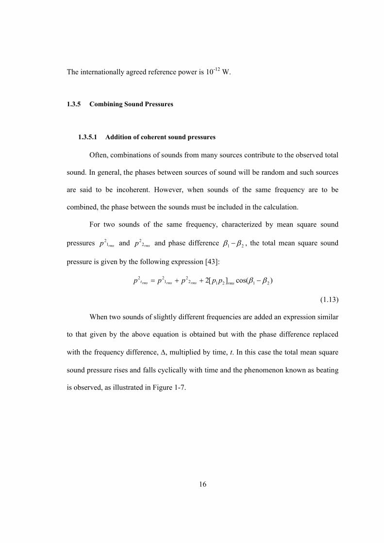
For two sounds of the same frequency, characterized by mean square sound
pressures rmsp 12 and rmsp 2
2 and phase difference 21 , the total mean square sound
pressure is given by the following expression [43]:
)cos(][2 212122
122 rmst ppppp rmsrmsrms
(1.13)
When two sounds of slightly different frequencies are added an expression similar
to that given by the above equation is obtained but with the phase difference replaced
with the frequency difference, , multiplied by time, t. In this case the total mean square
sound pressure rises and falls cyclically with time and the phenomenon known as beating
is observed, as illustrated in Figure 1-7.

17
Figure 1-7 Illustration of beating.
1.3.5.2 Addition of incoherent sound pressures (logarithmic addition)
When bands of noise are added and the phases are random, the limiting form of
the previous equation reduces to the case of addition of incoherent sounds; that is [43]:
rmsrmsrms ppp t 22
122
(1.14)
Incoherent sounds add together on a linear energy (pressure squared) basis. A
simple procedure which may easily be performed on a standard calculator will be
described. The procedure accounts for the addition of sounds on a linear energy basis and
their representation on a logarithmic basis. Note that the division by 10 in the exponent is
because the process involves the addition of squared pressures.
It should be noted that the addition of two or more levels of sound pressure has a
physical significance only if the levels to be added were obtained in the same measuring
point.

18
Example
Assume that three sounds of different frequencies (or three incoherent noise
sources) are to be combined to obtain a total sound pressure level. Let the three sound
pressure levels be (a) 90 dB, (b) 88 dB and (c) 85 dB. The solution is obtained by use of
the previous equation.
Solution:
For source (a):
8210/9021
2 101010 refref ppp rms
For source (b):
822
2 1031.6 refpp rms
For source (c):
823
2 1016.3 refpp rms
The total mean square sound pressure is,
823
22
21
22 1047.19 reft ppppp rmsrmsrmsrms
The total sound pressure level is,
9.92)1047.19(log10log10 8102
2
10 ref
t
ptp
pL rms dB
Alternatively, in short form,
9.92)101010(log10 10/8510/8810/9010 ptL dB
The Table of Figure 1-8 can be used as an alternative for adding combinations of
decibel values. As an example, if two independent noises with levels of 83 and 87 dB are
produced at the same time at a given point, the total noise level will be 87 + 1.5 = 88.5

19
dB, since the amount to be added to the higher level, for a difference of 4 dB between the
two levels, is 1.5 dB.
Figure 1-8 Table for combining decibel levels.
As can be seen in these examples, it is only when two noise sources have similar
acoustic powers, and are therefore generating similar levels, that their combination leads
to an appreciable increase in noise levels above the level of the noisier source. The
maximum increase over the level radiated by the noisier source, by the combination of
two random noise sources occurs when the sound pressures radiated by each of the two
sources are identical, resulting in an increase of 3 dB over the sound pressure level
generated by one source. If there is any difference in the original independent levels, the
combined level will exceed the higher of the two levels by less than 3 dB. When the
difference between the two original levels exceeds 10 dB, the contribution of the less
noisy source to the combined noise level is negligible; the sound source with the lower
level is practically not heard.

20
1.4 PROPAGATION OF NOISE
1.4.1 Free Field
A free field is a homogeneous medium, free from boundaries or reflecting
surfaces. Considering the simplest form of a sound source, which would radiate sound
equally in all directions from an apparent point, the energy emitted at a given time will
diffuse in all directions and, one second later, will be distributed over the surface of a
sphere of 340 m radius. This type of propagation is said to be spherical and is illustrated
in Figure 1-9.
Figure 1-9 A representation of the radiation of sound from a simple source in free field.
In a free field, the intensity and sound pressure at a given point, at a distance r (in
meters) from the source, is expressed by the following equation:
22
4 r
cWcIp
(1.15)
where ρ and c are the air density and speed of sound respectively.
21
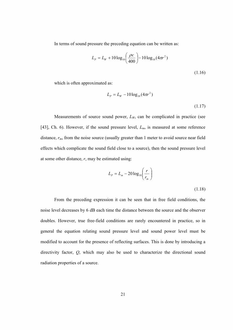
In terms of sound pressure the preceding equation can be written as:
)4(log10400
log10 21010 r
cLL WP
(1.16)
which is often approximated as:
)4(log10 210 rLL WP
(1.17)
Measurements of source sound power, LW, can be complicated in practice (see
[43], Ch. 6). However, if the sound pressure level, Lm, is measured at some reference
distance, rm, from the noise source (usually greater than 1 meter to avoid source near field
effects which complicate the sound field close to a source), then the sound pressure level
at some other distance, r, may be estimated using:
mmP r
rLL 10log20
(1.18)
From the preceding expression it can be seen that in free field conditions, the
noise level decreases by 6 dB each time the distance between the source and the observer
doubles. However, true free-field conditions are rarely encountered in practice, so in
general the equation relating sound pressure level and sound power level must be
modified to account for the presence of reflecting surfaces. This is done by introducing a
directivity factor, Q, which may also be used to characterize the directional sound
radiation properties of a source.

22
1.4.2 Directivity
Provided that measurements are made at a sufficient distance from a source to
avoid near field effects (usually greater than 1 meter), the sound pressure will decrease
with spreading at the rate of 6 dB per doubling of distance and a directivity factor, Q,
may be defined which describes the field in a unique way as a function solely of
direction.
A simple point source radiates uniformly in all directions. In general, however,
the radiation of sound from a typical source is directional, being greater in some
directions than in others. The directional properties of a sound source may be quantified
by the introduction of a directivity factor describing the angular dependence of the sound
intensity. For example, if the sound intensity I is dependent upon direction, then the mean
intensity, Iav, averaged over an encompassing spherical surface is introduced and,
24 r
WI av
(1.19)
The directivity factor, Q, is defined in terms of the intensity I in direction (, )
and the mean intensity [43]:
avI
IQ
(1.20)
The directivity index is defined as [43]:
QDI 10log10
(1.21)

23
1.4.3 Reflection effects
The presence of a reflecting surface near to a source will affect the sound radiated
and the apparent directional properties of the source. Similarly, the presence of a
reflecting surface near to a receiver will affect the sound received by the receiver. In
general, a reflecting surface will affect not only the directional properties of a source but
also the total power radiated by the source. As the problem can be quite complicated the
simplifying assumption is often made and will be made here, that the source is of
constant power output which means that its output sound power is not affected by
reflecting surfaces (see [43] for a more detailed discussion).
For a simple source near to a reflecting surface outdoors ([43], Ch. 5):
cQ
rp
Q
rIW rms
2
22 44
(1.22)
which may be written in terms of levels as
DIr
Lr
QLL WWP
210210 4
1log10
4log10
(1.23)
For a uniformly radiating source, the intensity I is independent of angle in the
restricted region of propagation, and the directivity factor Q takes the value listed in the
Table of Figure 1-10. For example, the value of Q for the case of a simple source next to
a reflecting wall is 2, showing that all of the sound power is radiated into the half-space
defined by the wall.

24
Figure 1-10 Table of Directivity factors for a simple source near reflecting surfaces.
1.4.4 Reverberant fields
Whenever sound waves encounter an obstacle, such as when a noise source is
placed within boundaries, part of the acoustic energy is reflected, part is absorbed and
part is transmitted. The relative amounts of acoustic energy reflected, absorbed and
transmitted greatly depend on the nature of the obstacle. Different surfaces have different
ways of reflecting, absorbing and transmitting an incident sound wave. A hard, compact,
smooth surface will reflect much more, and absorb much less, acoustic energy than a
porous, soft surface.
If the boundary surfaces of a room consist of a material which reflects the incident
sound, the sound produced by a source inside the room - the direct sound - rebounds from
one boundary to another, giving origin to the reflected sound. The higher the proportion
of the incident sound reflected, the higher the contribution of the reflected sound to the
total sound in the closed space.

25
This "built-up" noise will continue even after the noise source has been turned off.
This phenomenon is called reverberation and the space where it happens is called a
reverberant sound field, where the noise level is dependent not only on the acoustic
power radiated, but also on the size of the room and the acoustic absorption properties of
the boundaries. As the surfaces become less reflective, and more absorbing of noise, the
reflected noise becomes less and the situation tends to a "free field" condition where the
only significant sound is the direct sound. By covering the boundaries of a limited space
with materials which have a very high absorption coefficient, it is possible to arrive at
characteristics of sound propagation similar to free field conditions. Such a space is
called an anechoic chamber, and such chambers are used for acoustical research and
sound power measurements.
In practice, there is always some absorption at each reflection and therefore most
work spaces may be considered as semi-reverberant.
The phenomenon of reverberation has little effect in the area very close to the
source, where the direct sound dominates. However, far from the source, and unless the
walls are very absorbing, the noise level will be greatly influenced by the reflected, or
indirect, sound. The sound pressure level in a room may be considered as a combination
of the direct field (sound radiated directly from the source before undergoing a reflection)
and the reverberant field (sound which has been reflected from a surface at least once)
and for a room for which one dimension is not more than about five times the other two,
the sound pressure level generated at distance r from a source producing a sound power
level of LW may be calculated using ([43], Ch. 7):

26
Sr
QLL WP
)1(4
4log10
210
(1.24)
Where is the average absorption coefficient of all surfaces in the room.
1.4.5 Types of Noise
Noise may be classified as steady, non-steady or impulsive, depending upon the
temporal variations in sound pressure level (see ISO 12001). The various types of noise
and instrumentation required for their measurement are illustrated in the Table of Figure
1-11.
Steady noise is a noise with negligibly small fluctuations of sound pressure level
within the period of observation. If a slightly more precise single-number description is
needed, assessment by NR (Noise Rating) curves may be used.
A noise is called non-steady when its sound pressure levels shift significantly
during the period of observation. This type of noise can be divided into intermittent noise
and fluctuating noise.
Fluctuating noise is a noise for which the level changes continuously and to a
great extent during the period of observation.
Tonal noise may be either continuous or fluctuating and is characterized by one
or two single frequencies. This type of noise is much more annoying than broadband
noise characterized by energy at many different frequencies and of the same sound
pressure level as the tonal noise.

27
Figure 1-11 Table of noise types and their measurement.

28
Intermittent noise is noise for which the level drops to the level of the
background noise several times during the period of observation. The time during which
the level remains at a constant value different from that of the ambient background noise
must be one second or more.
This type of noise can be described by
o � the ambient noise level
o � the level of the intermittent noise
o � the average duration of the on and off period.
In general, however, both levels are varying more or less with time and the
intermittence rate is changing, so that this type of noise is usually assimilated to a
fluctuating noise as described below, and the same indices are used.
Impulsive noise consists of one or more bursts of sound energy, each of a
duration less than about 1s. Impulses are usually classified as type A and type B as
described in Figure 1-12, according to the time history of instantaneous sound pressure
(ISO 10843). Type A characterizes typically gun shot types of impulses, while type B is
the one most often found in industry (e.g., punch press impulses). The characteristics of
these impulses are the peak pressure value, the rise time and the duration (as defined in
Figure 1-12) of the peak.

29
Figure 1-12 Idealized waveforms of impulse noises. Peak level = pressure difference AB; rise time = time difference AB; A duration = time difference AC; B duration = time difference AD ( + EF when a reflection is present). (a) Explosive generated noise. (b) Impact generated noise.


31
2 AERODYNAMIC SOUND
In contrast to computational aerodynamics, which has advanced to a fairly
mature state, computational aeroacoustics (CAA) has only recently emerged as a
separate area of study. Due to the nonlinearity of the governing equations it is very
difficult to predict the sound production of fluid flows. This sound production occurs
typically at high speed flows, for which nonlinear inertial terms in the equation of
motion are much larger than the viscous terms (high Reynolds numbers). As sound
production represents only a very minute fraction of the energy in the flow the direct
prediction of sound generation is very difficult. This is particularly dramatic in free
space and at low subsonic speeds. The fact that the sound field is in some sense a small
perturbation of the flow, can, however, be used to obtain approximate solutions. Aero-
acoustics provides such approximations and at the same time a definition of the
acoustical field as an extrapolation of an ideal reference flow. The difference between
the actual flow and the reference flow is identified as a source of sound. This idea was
introduced by Lighthill who called this an analogy. While in acoustics of quiescent
media it is rather indifferent whether we consider a wave equation for the pressure or the
density, in aero-acoustics the choice of a different variable corresponds to a different
choice of the reference flow and hence to another analogy [47].
32
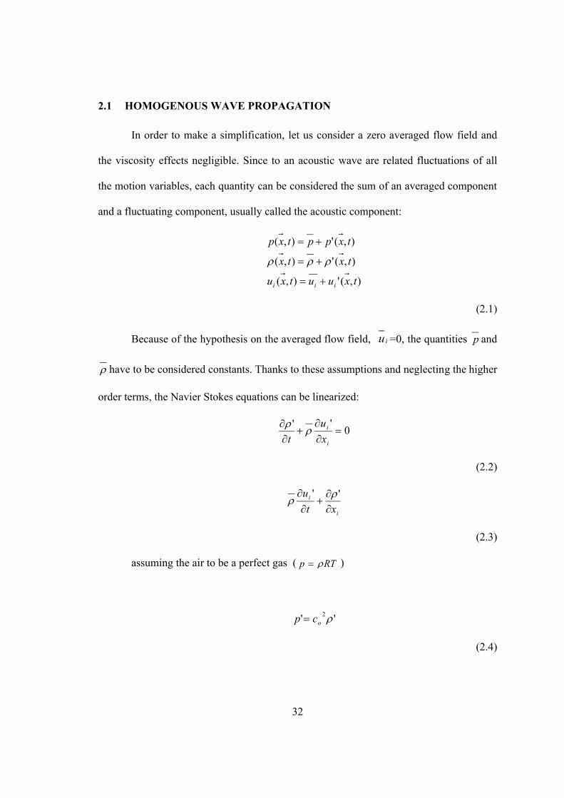
2.1 HOMOGENOUS WAVE PROPAGATION
In order to make a simplification, let us consider a zero averaged flow field and
the viscosity effects negligible. Since to an acoustic wave are related fluctuations of all
the motion variables, each quantity can be considered the sum of an averaged component
and a fluctuating component, usually called the acoustic component:
),('),(
),('),(
),('),(
txuutxu
txtx
txpptxp
iii
(2.1)
Because of the hypothesis on the averaged flow field, iu =0, the quantities p and
have to be considered constants. Thanks to these assumptions and neglecting the higher
order terms, the Navier Stokes equations can be linearized:
0''
i
i
x
u
t
(2.2)
i
i
xt
u
''
(2.3)
assuming the air to be a perfect gas ( RTp )
'' 2ocp
(2.4)

33
Taking the time derivative of the 2.2, and the divergence of 2.3 and then
subtracting the first from the second:
0''
2
2
2
2
ix
p
t
(2.5)
Applying the relation 2.4 to the equation 2.5 it is possible to obtain an
homogeneous equation for the pressure fluctuation:
0''1
2
2
2
2
2
io x
p
t
p
c
(2.6)
In a mono-dimensional case a solution of this equation is:
)()(),( 21 xtcfxtcftxp oo
(2.7)
where 1f and 2f are two arbitrarily functions.
2.2 NON-HOMOGENEOUS WAVE PROPAGATION
The theories that describes the aerodynamic sound often lead to a non-
homogeneous wave equation. For a better understanding of these theories, the purpose of
this section is to give a brief introduction to the way of solving a non-homogenous wave
equation. In general a wave equation assumes the following form:
),(1 2
2
2
2 txfptco
(2.8)
34
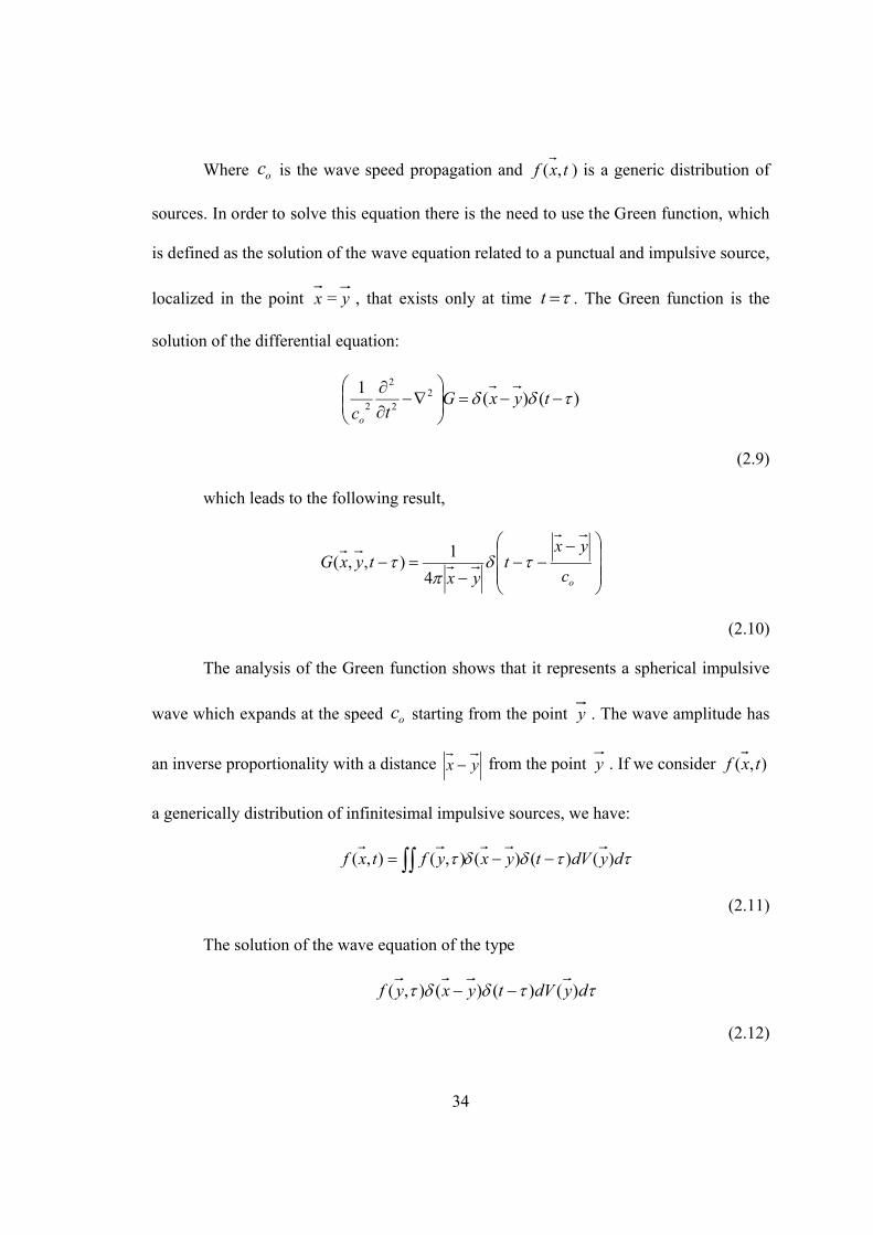
Where oc is the wave speed propagation and txf ,( ) is a generic distribution of
sources. In order to solve this equation there is the need to use the Green function, which
is defined as the solution of the wave equation related to a punctual and impulsive source,
localized in the point x = y , that exists only at time t . The Green function is the
solution of the differential equation:
)()(1 2
2
2
2
tyxGtco
(2.9)
which leads to the following result,
oc
yxt
yxtyxG
4
1),,(
(2.10)
The analysis of the Green function shows that it represents a spherical impulsive
wave which expands at the speed oc starting from the point y . The wave amplitude has
an inverse proportionality with a distance yx from the point y . If we consider ),( txf
a generically distribution of infinitesimal impulsive sources, we have:
dydVtyxyftxf )()()(),(),(
(2.11)
The solution of the wave equation of the type
dydVtyxyf )()()(),(
(2.12)

35
is given by the wave
dydVtyxGyf )(),,(),(
(2.13)
Summing all the contributions, it’s possible to obtain a solution for the non-
homogeneous wave equation:
dydVyx
c
yxtyf
dydVc
yxt
yx
yfdydVtyxGyftxp
o
o
)(
,
4
1
)(),(
4
1)(),,(),(),(
(2.14)
2.3 LIGHTHILL’S ANALOGY
For a long period since Lighthill’s ([1],1952) classical paper appeared,
aeroacoustic computation has focused on solution of his acoustic analogy equation or
variations thereof. In brief, Lighthill devised an arrangement of the continuity and
momentum equations of fluid mechanics where all terms not appearing in the linear-wave
operator are grouped into a double divergence of a source-like term now known as the
Lighthill stress tensor. The result of the aforementioned manipulations is an equation
featuring the wave operator (operating on the density perturbation) on the left-hand side
and with all nonlinear effects accounted for by the Lighthill stress tensor:
ji
ij
i
o xx
T
xc
t
2
2
22
2
2
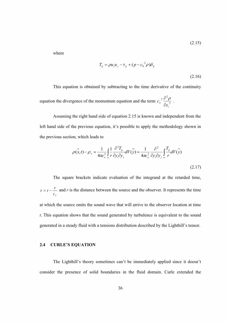
36
(2.15)
where
ijijjiij cpuuT )( 20
(2.16)
This equation is obtained by subtracting to the time derivative of the continuity
equation the divergence of the momentum equation and the term2
22
i
ox
c
.
Assuming the right hand side of equation 2.15 is known and independent from the
left hand side of the previous equation, it’s possible to apply the methodology shown in
the previous section, which leads to
)(4
1)(
1
4
1),(
2
2
2
2ydV
r
T
yycydV
yy
T
rctx ij
jioji
ij
oo
(2.17)
The square brackets indicate evaluation of the integrand at the retarded time,
oc
rt and r is the distance between the source and the observer. It represents the time
at which the source emits the sound wave that will arrive to the observer location at time
t. This equation shows that the sound generated by turbulence is equivalent to the sound
generated in a steady fluid with a tensions distribution described by the Lighthill’s tensor.
2.4 CURLE’S EQUATION
The Lighthill’s theory sometimes can’t be immediately applied since it doesn’t
consider the presence of solid boundaries in the fluid domain. Curle extended the

37
Lighthill’s theory in order to consider these effects, [3]. The general integral of the non
homogeneous wave equation in a limited domain is
)(111
4
1)(
1
4
1),(
2
2
2ydS
n
r
rcn
r
rnrydV
yy
T
rctx
Soji
ij
o
o
(2.18)
where n is the unit versor orthogonal to the surface, pointing to the fluid domain.
Starting from this solution, Curle obtains a formulation analogous to Lighthill’s, with the
addition of an integration on an integration on the surface immersed in the fluid domain.
To obtain this formulation the integrals of the previous equation have been rearranged.
For the volume integration we have:
dydVtyxGyyy
TydV
yy
T
rc V ji
ij
ji
ij
o
)(),(),()(1
4
122
2
(2.19)
Since the argument of the Green function is yx it is possible to say that
ii x
G
y
G
. Using the divergence theorem we have:
dydVtyxGx
yy
T
dydStyxGyy
TndydVtyxG
yy
y
T
dydVtyxGyy
T
yydV
yy
T
rc
V ii
ij
S i
iji
V ii
ij
V i
ij
iji
ij
o
)(),(),(
)(),(),()(),(),(
)(),(),()(1
4
12
2
(2.20)
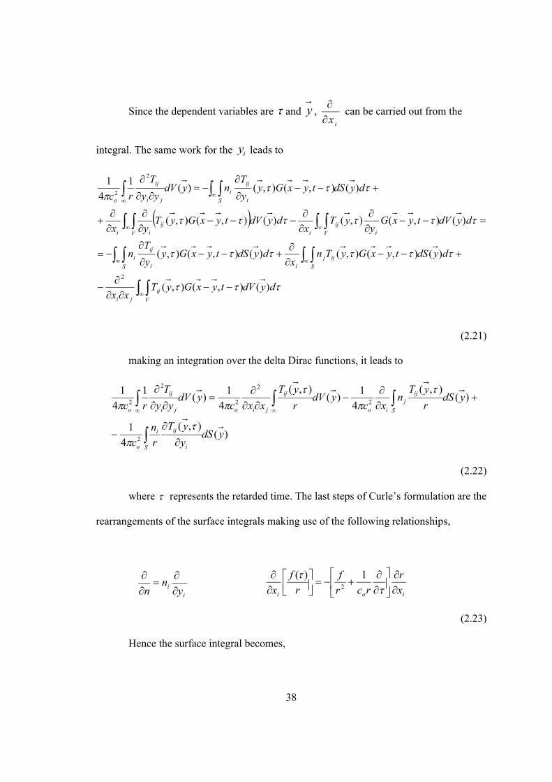
38
Since the dependent variables are and y , ix
can be carried out from the
integral. The same work for the iy leads to
dydVtyxGyTxx
dydStyxGyTnx
dydStyxGyy
Tn
dydVtyxGy
yTx
dydVtyxGyTyx
dydStyxGyy
TnydV
yy
T
rc
V
ijji
S
ijjiS i
iji
V iij
iij
V ii
S i
iji
ji
ij
o
)(),(),(
)(),(),()(),(),(
)(),(),()(),(),(
)(),(),()(1
4
1
2
2
2
(2.21)
making an integration over the delta Dirac functions, it leads to
)(),(
4
1
)(),(
4
1)(
),(
4
1)(
1
4
1
2
2
2
2
2
2
ydSy
yT
r
n
c
ydSr
yTn
xcydV
r
yT
xxcydV
yy
T
rc
S i
iji
o
S
ijj
io
ij
jioji
ij
o
(2.22)
where represents the retarded time. The last steps of Curle’s formulation are the
rearrangements of the surface integrals making use of the following relationships,
ii y
nn
ioi x
r
rcr
f
r
f
x
1)(
2
(2.23)
Hence the surface integral becomes,

39
SS
iji
ii
iji
Sioii
iji
Sioii
iSo
ydSr
n
xydS
yr
nydS
y
r
rcy
r
ryrn
ydSy
r
rcy
r
ryrnydS
n
r
rcn
r
rnr
)()()(111
)(111
)(111
2
22
(2.24)
which leads to
)(4
1
)(4
1)(
4
1),(
2
2
2
2
2
2
ydScTyr
n
c
ydScTr
n
xcydV
r
T
xxctx
ijoij
S i
i
o
ijoij
S
j
io
ij
jioo
(2.25)
From the definition of the Lighthill tensor and from the momentum equation it is
possible to obtain
t
u
r
ncT
yr
n iiijoij
i
i
2
(2.26)
leading to
)(4
1
)(4
1)(
4
1),(
2
2
2
2
ydSr
nu
c
ydSpuur
n
xcydV
r
T
xxctx
S
ii
o
ijijji
S
j
io
ij
jioo
(2.27)
For solid surfaces the velocity on the surface vanishes, hence the final result of
Curle’s equation is:

40
)(4
1)(
4
1),(
2
2
2ydSp
r
n
xcydV
r
T
xxctx ijij
S
j
io
ij
jioo
(2.28)
2.5 THE FFOWCS WILLIAMS & HAWKINGS’S ANALOGY
A generalization of Lighthill’s theory to include aerodynamic surfaces in motion,
proposed by Ffowcs Williams & Hawkings ([6], 1969) has provided the basis for a
significant amount of analysis of the noise produced by rotating blades, including
helicopter rotors, propeller blades, and fans,
The Ffowcs Williams & Hawkings (FW-H) theory includes surface source terms
in addition to the quadrupole-like source introduced by Lighthill. The surface sources are
generally referred to as thickness (or monopole) sources and loading (or dipole) sources.
They are also often termed linear in that no explicitly nonlinear terms appear in
them and the propagation from the surfaces has no nonlinear component. It should be
noted, however, that the loading sources, which consist of surface pressures, may be
computed using nonlinear aerodynamic methods.
The following work is the same reported by Crighton [4].
Let us consider a surface S immersed in a fluid, which moves at a speed equal to
iv and defined by the function ),( txf :
Soutsidetxf
Sontxf
Sinsidetxf
0),(
0),(
,0),(

41
(2.29)
Typically S is the surface of the body. However it is not strictly necessary since
the theory developed in this section is not only true for surfaces that limit the body but
also for surfaces that simply contain the body.
The ),( txf function satisfies the following,
0
ii x
fv
t
f
(2.30)
since the density at an infinite distance from the body is constant, it’s possible to
obtain
0
i
io
x
u
t
(2.31)
Multiplying the continuity equation by the Heaviside function:
0)()(
fHx
ufH
t i
io
(2.32)
or equivalently
ii
oi
io ux
fH
t
fH
x
fHu
t
fH
)()()()(
(2.33)
Remembering the proprieties of the Heaviside function:

42
)()(
)()()(
ffQfx
fvuv
fux
f
t
f
x
fHu
t
fH
iiiio
ii
oi
io
(2.34)
where it has been considered that fnx
fi
i
, while for Q it has been considered
that
iiiio nvuvQ
(2.35)
and it has to be considered like a source term which exist only on the surface S.
It’s possible to rearrange the momentum equation in the same way, leading to
)()(
)()()(
)()()()()()(
ffFfx
f
x
fp
x
fvuu
fx
f
x
fp
x
fuu
t
fu
x
fH
x
fHp
x
fHuu
t
fHu
x
fH
x
fpH
x
fHuu
t
fHu
ij
ijj
ijj
iii
jij
jij
jjii
iij
i
jjii
i
ij
ij
jii
(2.36)
where
iijijjjii npvuuF
(2.37)

43
t
ffQ
x
ffF
xx
fHTfH
xc
t i
i
ji
ij
o
i
o
)()()(
)('2
2
22
2
2
(2.38)
where
ijooijjiij cpuuT 2'
(2.39)
looks similar to Lighthill’s tensor and o does not affect the sound generation,
since it is a constant.
The solution of this wave equation is given by
dydVrc
tcryffQ
t
dydVrc
tcryffF
x
dydVrc
tcryfHT
xxtx
o
o
o
oi
i
o
oij
jio
)(4
))((),()(
)(4
))((),()(
)(4
))((),()(),(
2
(2.40)
In the case of a moving surface, the ),( txf function and the sources terms are
better expressed in a surface reference system. If we refer to the new reference system
with*
y , it follows that:
iii
iii
vuu
vyy
*
*
(2.41)
The Jacobean of this transformation is equal to unit. Since y and r are now both
functions of , we have to consider the following variable substitution to integrate on :

44
dcrdg
tcrg o
)/(
)(
0
(2.42)
where
jjj
iii
ii
iii
i
vlvr
yxy
yx
yxy
y
rr
22
)(2
(2.43)
Where jl is the j-component of a unit versor pointing from the source to the
observer location. Hence we have,
dvlcdg jjo
(2.44)
Applying the variable substitution to the previous solution it yields:
dydVvlcrc
gyffQ
t
dydVvlcrc
gyffF
x
dydVvlcrc
gyfHT
xxtx
jjoo
jjooi
i
jjoo
ij
jio
)(4
)(),()(
)(4
)(),()(
)(4
)(),()(),(
*****
*****
****'
2
(2.45)
Where the source terms in the new reference system are
iiio nuvQ **
(2.46)
iijijiiji npvuuF ****
(2.47)

45
ijooijjjiiij cpvuvuT 2****' ))((
(2.48)
It has to be noticed that *ij = ij . Integrating on dg,
dydVcvlr
ffQ
tcdydV
cvlr
ffF
xc
dydVcvlr
fHT
xxctx
ojjoojj
i
io
ojj
ij
jio
o
)(1
)(
4
1)(
1
)(
4
1
)(1
)(
4
1),(
****
2
****
2
***'2
2
(2.49)
Where the integrand functions have to be evaluated at g=0 or at ocrt .
Integrating on the -functions it is possible to obtain the final formulation of the
wave equation
dydScvlr
Q
tcdydS
cvlr
F
xc
dydVcvlr
T
xxctx
ojjoojj
i
io
ojj
ij
jio
o
)(14
1)(
14
1
)(14
1),(
**
2
**
2
**'2
2
(2.50)
For a solid surface we have, ui* =0, thus
iio nvQ *
(2.51)
iijiji npF **
(2.52)

46
The Q* term is equal to zero in the case of steady surface. In the case of a steady
surface and S equal to the body surface the FW-H’s equation reduces to the Curle
equation.
2.6 CONSIDERATIONS ON THE SOUND GENERATED
AERODYNAMICALLY
A first way to proceed is the direct calculation of the acoustic pressure through a
direct simulation of the compressible fluid.
Typically this method is not widely used since it is too computationally
expensive, requiring higher order numerical schemes to reduce the dissipation and the
dispersion of the acoustic waves, and complicated boundary conditions. For example,
non-reflecting boundary conditions (NRBCs) may be required to avoid unphysical
reflections contaminating the computational domain. Other methods exist to avoid this
phenomenon when NRBCs are not available, including the use of purposefully
dissipative grid regions close to domain boundaries.
Alternatively to make an estimation of the aerodynamically generated sound, the
acoustic analogy with a turbulence model simulation for computing the sources can be
used. This last approach needs sophisticated turbulence models since the good resolution
of the flow field is the primary requirement to obtain an accurate prediction of sound
sources. Let us investigate the advantages and the weaknesses of the acoustic analogy. In
obtaining Lighthill’s equation, from a simple manipulation of the Navier-Stokes
Equations, we have supposed that 2
22
i
ox
c
was independent from the left hand side of

47
equation 2.15. This hypothesis is never satisfied since the Lighthill’s tensor is dependent
on the density itself. In other word the acoustic analogy leads to a good result if the
turbulent flow field and the acoustics one are not coupled, that is when we can neglect the
effect of acoustics on the flow. The acoustic analogies divide the generation of sound
from the propagation, computing the latter by a wave operator.
Let us consider the Lighthill’s tensor, 2.16,
ijijjiij cpuuT )( 20
(2.16)
The dominant term, if the flow is turbulent, is the fluctuating Reynolds tensor,
hence it’s possible to consider
jiij uuT
(2.54)
The Reynolds tensor represents a stress related to the particles exchanges in the
fluid. Hence this tensor has an effect similar to the viscous stress. In the same way, from
a generation of sound point of view, the fluctuating Reynolds tensor has an effect similar
to the viscous stresses and is relatively more important than them.
The double divergence of the Reynolds fluctuating tensor, as noticed by Howe
[5], can be rearranged for low-Mach number as
)(2
vdivxx
uuo
ji
jio
(2.55)
This relationship shows that the vorticity is the main cause of the aerodynamic
sound and the main acoustic sources are related to surfaces.

48
A better evaluation of the wall effect can be made analyzing the order of
magnitude of the various terms of the FW-H equation
dydScvlr
Q
tcdydS
cvlr
F
xc
dydVcvlr
T
xxctx
ojjoojj
i
io
ojj
ij
jio
o
)(14
1)(
14
1
)(14
1),(
**
2
**
2
**'2
2
(2.56)
If S corresponds to the body surface, the three terms of the right hand side of
previous equation are related to different causes. The first term corresponds to the sound
produced by turbulent structures and from dimensional analysis it results
4
24),( U
rc
Dtxp
(2.57)
and the sound intensity is
8522
22
16
),()( U
cr
D
c
txprI
oo
(2.58)
or equivalently
53)( MUrI
(2.59)
known as the Lighthill’s v8-law
The second term represents the component due to the forces that act on the
surface, for which the pressure fluctuations can be estimated as

49
3
4),( U
rc
Dtxp
(2.60)
and the sound intensity results in
6322
22
16
),()( U
cr
D
c
txprI
oo
(2.61)
or equivalently
33)( MUrI
(2.62)
The third term is equal to zero if the surface S is attached to the body and this last
one is not affected by vibration.
Comparing the first and the second term it is possible to say that the contribution
of the surface sources (second term) is dominant.
Another approximation in an acoustic analogy is the use of a linear wave operator,
in fact this one describes well the wave propagation only for low speed cases (M<0.4).
2.7 FLUENT IMPLEMENTATION OF ACOUSTIC ANALOGY
The commercial code FLUENT estimates the acoustic pressure through the use of
the Ffowcs Williams and Hawkings Analogy, neglecting the terms related to the
Lighthill’s tensor as they are relatively unimportant compared to the other source terms..
The formulation used is the one of Farassat and Brentner:

50
dSMr
LLMMaMrL
c
dSMr
LLMMcMrUc
dSMr
LUUc
cptxp
S r
Mrrrr
S r
Mrrrn
S r
rnno
32
20
0
32
200
200
0
)1(
))((1
)1(
))((
)1(
)(1)),((4
(2.63)
where
)(0
iiii vuvU
(2.64)
)( nnijiji vuunPL
(2.65)
ijk
k
i
j
j
iijij x
u
x
u
x
upP
3
2 ; iiM MLL
(2.66)
and Mi is the Mach number estimated using the velocity in the i-direction .
This formulation is equivalent to the FW-H proposed in the section 2.5 with all
the derivatives carried inside the integrals.
All the integrand functions have to be evaluated at the retarded time. The sources
have to be evaluated in a time instant dependent on their position. This causes the
complication to save the entire time history of the fluid-dynamic variables that constitute
the acoustic sources. To clarify let us consider two different punctual sources located at a
certain distance from observer and indicated by r1 and r2.
51
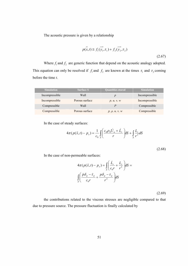
The acoustic pressure is given by a relationship
),(),(),( 222111 yfyftxp
(2.67)
Where 1f and 2f are generic function that depend on the acoustic analogy adopted.
This equation can only be resolved if 1f and 2f are known at the times 1 and 2 coming
before the time t.
Simulation Surface S Quantities stored Simulation
Incompressible Wall p Incompressible
Incompressible Porous surface p, u, v, w Incompressible
Compressible Wall P Compressible
Compressible Porous surface p, ρ, u, v, w Compressible
In the case of steady surfaces:
dSr
LdS
r
LUc
cptxp
S
r
S
rno
200
0
1)),((4
(2.68)
In the case of non-permeable surfaces:
S
ijijijij
S
rro
dSr
p
rc
p
dSr
L
rc
Lptxp
20
20
)),((4
(2.69)
the contributions related to the viscous stresses are negligible compared to that
due to pressure source. The pressure fluctuation is finally calculated by

52
f
f
N
f
ijijo A
r
p
rc
pptxp
f
,12
04
1),(
(2.70)

53
3 AEROACOUSTICS SIMULATION APPROACHES
As we have seen in the previous Chapters, Aeroacoustics is a subtopic of
acoustics pertaining to situations where sound is generated by fluid flow.
In contrast, Vibro-Acoustics is the field pertaining to sound caused by vibrating
objects such as the diaphragm of a speaker.
Figure 3-1 Pressure fluctuations on an aircraft landing gear.
There are four primary entities in any aeroacoustics problem: the acoustic
medium, sources (flow), sound, and receivers [48]. The acoustic medium in most
problems is the air and sound sources are the flow structures that induce pressure
fluctuations in air.
The sources can be in the form of any unsteady flow structure such as vortices,
shear-layers, or turbulent eddies. Sounds are pressure waves travelling through the

54
acoustic medium and the receiver is the observer of these sound waves, which can be a
microphone or the human ear in practice.
Computational Fluid Dynamics (CFD) is an essential part of aeroacoustics
simulations since it is the only viable way to simulate all varieties of source flow
structures such as vortices, shear-layers, turbulent eddies, and others. There are four
primary ways to model sound generation and transmission with a general purpose CFD
solver. In decreasing order of accuracy, extent of applicability, and computational effort
they are:
· Computational Aeroacoustics (CAA)
· Coupling of CFD and wave-equation-solver
· Using integral acoustic models
· Acoustics source strength estimation from local turbulence scales
3.1 COMPUTATIONAL AEROACOUSTICS
Computational Aeroacoustics (CAA) is the most comprehensive way to simulate
aeroacoustics. It does not rely on any model and therefore in aeroacoustics its position is
analogous to that of Direct Numerical Simulation (DNS) in the field of turbulent flow
simulation. CAA essentially is a general transient simulation of the entire fluid region
encompassing the sources, receivers, and the entire sound transmission path in between.
The simulation computes pressure disturbances created in the source regions by
rigorously calculating the time-varying flow structure in these regions. It also simulates
sound transmission by actually resolving the pressure waves travelling in the fluid.
Finally at the receiver location it records the time-varying static pressure. This is the

55
sound signal heard by the receiver. As can be imagined, such a simulation needs to
incorporate a range of physical phenomena.
It is essential to properly capture turbulence in the source region in order to
predict source pressure fluctuations accurately. Likewise, fluid compressibility needs to
be incorporated in the simulation for properly simulating the transmission of sound
(pressure) waves. The most general equations that govern all these physical phenomena
in a fluid region are the Navier-Stokes equations. A CAA simulation therefore involves
obtaining a complete transient solution of the Navier-Stokes equations on a fluid domain
encompassing the sound sources, receivers, and the transmission path in between.
Though CAA is the most general and accurate theoretical approach for simulating
aeroacoustics, it is unrealistic for most engineering problems due to a number of practical
limitations, as range of scales and range of pressure.
3.1.1 Range of Scales
A CAA simulation needs to resolve a wide range of both time and length scales.
Sound frequencies audible to the human ear span from 20 Hz to 20,000 Hz. To
properly simulate the highest frequency, it is necessary to use a time-step (sampling
duration) nearly 10-20 times smaller than the time period of that frequency. Likewise, for
accurately capturing the lowest frequency, at least 10 time periods of that frequency need
to be simulated. Thus the real time to be simulated is more than 100,000 times greater
than the time-step size, necessitating many time-steps. Similarly, the simulation needs to
be carried out at a very fine spatial resolution to capture both the generation and
transmission of high frequency sound. The source of high pitch sound often are tiny
micron sized turbulent eddies. Also the wavelength of high frequency sound waves is of

56
the order of a few cm. Yet the computational domain has to span large distances to
encompass the sources and receivers. For instance, for sound produced by an aircraft jet,
the distance between the source (jet) and the receiver (an observer standing on the
ground) is many kilometres. In effect to resolve such a wide range of length and time
scales a CAA simulation needs a massive number of computational cells, a very short
time-step and to model for a relatively long time period. Such computational expense is
unrealistic for most practical applications with current state-of-the-art computing
resources.
3.1.2 Range of Pressures
Another complication in CAA simulations is the wide range of pressures
involved. Typically, pressure fluctuations are in the range of a few to a few hundred kPa
in a transient flow such as that in the wake of a cylinder. On the other hand, sound
pressure is of the order of milli-Pascals. As seen in Figure 3.2, sound pressure
corresponding to a 60 dB sound pressure level (SPL) is 20 mPa. A CAA simulation
therefore needs to keep track of pressures that differ by a factor of 106 or more. Thus the
accuracy of the simulation becomes highly sensitive to truncation error. Even second
order discretization schemes typically used for flow computations rapidly deteriorate the
tiny sound pressure component in the overall pressure.

57
Figure 3-2 Relation between sound pressure (Pa) and sound pressure level (dB).
Computationally expensive higher order schemes are essential to accurately
transport the sound signal through the computational domain. However, even 6th or 7th
order schemes are unable to accurately transport small sound signals over large distances
encountered in many practical problems.
3.2 CFD-WAVE-EQUATION-SOLVER COUPLING
Computational Aeroacoustics (CAA) is prohibitively expensive for most practical
problems due to the large difference in time, length, and pressure scales involved in
sound generation and transmission. However, this large difference in scales provides a
good opportunity of greatly simplifying the simulation by splitting the problem into two
parts and modeling them separately. Sound generation involves small length scales and
tiny pressure scales. Since the scales involved in these two phenomena differ so
significantly, the two can be treated separately. The Navier-Stokes equations govern the
first part while the latter is governed by the wave equation.

58
Splitting the problem into two parts thus is advantageous in several ways. First,
the expensive high-resolution, transient solution of Navier-Stokes equations can be
restricted only to a small area close to the source regions. Secondly, the computational
grid can be optimized to suit flow simulation requirements close to the source region, and
to meet the transmission simulation requirements in the transmission region.
Further, this approach allows easier use of analytical models for the source as well
as the transmission part, e.g. the analytical model proposed by Ffowcs-Williams and
Hawkings can be used for the transmission.
However, splitting the problem into two parts this way has inherent limitations.
First, the approach is valid only when the scales involved in sound generation and
transmission are distinctly different. Secondly, this approach cannot effectively handle
the backward effect of sound on the flow field. For example, Ffowcs-Williams and
Hawkings approach cannot be used to simulate whistles in automotive air intake
manifolds since a whistle is caused by resonance between a shear-layer fluctuating in the
mouth of a cavity and the sound waves reflecting off the cavity bottom.
Solving the wave equation using the Boundary Element Method can take into
account reflection and scattering. Generally it can be used in closed domain too or when
obstacles or reflective surfaces are present in the propagation region, but it can not still
handle the backward effect of sound on the flow field. For example, a CFD simulation
can be used to calculate the time varying pressure signals at a multitude of points on the
acoustics source surfaces as dipole boundary conditions, which will be used by the BEM
solver performing the computation of the radiated acoustic field in the region of interest.

59
3.3 INTEGRAL ACOUSTICS METHODS
The approach of splitting the flow and sound fields from each other and solving
them separately can be simplified further if the receiver is in straight, unobstructed view
from every individual point of the source region. Sound transmission from a source point
to the receiver can be computed by simple analytical formulation. By integration of such
sound transmission over all points on the source surface, the complete sound signal at the
receiver can be obtained. As we saw in the previous Chapter, the Lighthill Acoustic
Analogy provides the mathematical foundation for such an integral approach. The
Ffowcs-Williams and Hawkings (FW-H) method extends the analogy to cases were solid,
permeable, or rotating surfaces are sound sources, and is the most complete formulation
of the acoustic analogy to date.
To compute sound with the FW-H method, one needs to perform a well-resolved
transient CFD simulation only in the source region. Flow quantities, such as pressure and
velocity are stored as functions of time on every point of every source surface during the
simulation. At the end, this source data is in the FW-H integral to compute sound at the
receiver. Since the FW-H is quite general and allows arbitrarily moving source surfaces,
it can also be applied to predicting noise radiating from fans.
3.4 SYNTHETIC NOISE GENERATION METHOD
All the three methods described so far require well-resolved transient CFD
simulations since they aim at determining the actual time-varying sound pressure signal
at the receiver and from that the sound spectrum. In several practical engineering

60
situations one needs to determine locations and relative strengths of sound sources rather
than such spectra at the receivers. If the sound is broadband, i.e. without any prominent
tones characterized by sharp peaks in spectrum, then source strengths can be evaluated
with reasonable accuracy from the time-averaged structure of the turbulent flow in the
source regions.
Figure 3-3 Iso-surface of Lilley’s acoustic source (total) strength around a generic sedan [48].
Turbulence is the primary cause of sound in aeroacoustics, therefore, in a broad
sense, regions of the flow field where turbulence is strong are louder sources of sound.
To-date there are a number of analytical models which synthesize sound at points in the
flow field from local flow and turbulence quantities to estimate local sound source
strengths. These are collectively referred to as broad-band noise source models and are
based on an approach referred to as the synthetic noise generation method. The key
advantage of these models is that they require very modest computational resources
compared to the methods described in the previous sections. Broadband noise models
only need a steady state flow solution whereas the other methods essentially require well-
resolved transient flow solutions.

62
4 NOISE GENERATION MECHANISM
In the following section we will discuss in detail the mechanism of noise
generation for some typical problems of strong engineering interest. A good
understanding of the physics involved in sound generation is crucial when choosing the
models and methodologies to simulate it. This will also help in interpreting the results
obtained from a simulation and to figure out the limitations of the information we can get.
4.1 CAVITY NOISE
A typical example of Aeroacoustics is cavity noise. Air flowing past a cavity
produces a distinct sound. There are no moving parts in this case. The flow itself is the
source of sound. A shear layer establishes in the mouth of the cavity and oscillates at a
particular frequency causing pressure fluctuations to propagate away from the cavity
mouth that manifest as sound.
The flow over a cavity is characterized by a complex feedback process that can
lead to large-amplitude, self-sustained oscillations of the pressure, velocity, and density
fields in and around the cavity. The feedback process involves the growth and convection
of instability waves in the shear layer spanning the cavity, the generation of a large-
amplitude acoustic source associated with shear-layer impingement on the cavity trailing
edge, feedback of an acoustic disturbance to the separation edge, and conversion of the

63
feedback disturbance to shear-layer instability waves through a receptivity process,
Figure 4-1.
Figure 4-1 Triggering of vortex shedding.
Hence the process involves a time-dependent, quasi-periodic vortex shedding that
can interact with the acoustic resonance of the cavity which acts as a Helmholtz
resonator. When the frequency of the flow fluctuations is far from that of acoustic
resonance, the two phenomena are weakly coupled and can be treated independently.
However, when these two frequencies are close an intense energy exchange between the
driving flow oscillations and fluid inside the cavity can occur.
These strong oscillations are undesirable in many engineering applications as they
can induce structural vibration and fatigue, noise radiation, and drag on bodies possessing
the cavity. Cavity flows are pertinent to a wide range of real-world applications, ranging
from landing gear and weapons bays in aircraft to flow over ground vehicles. The
importance of cavity flows in these engineering applications is evidenced by the large
number of review articles on the subject.
The whole phenomena can be simplified by the following mechanical analogy of
a mass-spring-damped oscillator, Figure 4-2. The driving force in our case can be the
vortex shedding over the opening of the cavity, the mass M is the mass of the air in the
neck, the spring constant K corresponds to the elasticity of the air contained in the cavity,

64
the resistance R is related to the viscous and radiation losses through the neck of the
cavity and to the absorption and compliance of the walls.
Figure 4-2 Mechanical analogy of acoustic resonant cavity.
Figure 4-3 Acoustic cavity.
If we assume that the volume of the cavity is V, the length of the neck is L, the
speed of sound to be c, and S is the cross section area of the neck of the cavity as shown
in Figure 4-3, the frequency of the Helmholtz resonator can be shown to be:

65
VL
Scf H 2
(4.1)
A classic example of the use of CAA is the cavity noise that can be generated in
the cabin of a car, sometimes called aerodynamic buffeting. Buffeting is a wind noise of
high intensity and low frequency heard in a moving vehicle when a window or sunroof is
open. There are two sources of this sound (1) the transient vortex shedding in the wake of
the side view mirror and (2) a shear-layer flapping in the window or sun-roof opening.
Both sources contribute to side window buffeting while only the latter acts as a source of
sun-roof buffeting. Pressure fluctuations induced by these flow structures propagate in
the vehicle cabin and are heard by the driver and passengers. Consequently, the sources
and receivers are located fairly close to each other.
Two other characteristics of buffeting allow it to be modelled with CAA. First,
buffeting sound frequency is very low, in the range of 15 to 25 Hz. As a result the CAA
simulation can be conducted with a relative few number of large time-steps without
exorbitant computational expense. Secondly, buffeting sound pressure levels are very
high, often over 100 dB. Thus, the sound pressure fluctuation is fairly large (2 Pa as per
Figure 3-2) and can be captured accurately without undue truncation errors with usual
second order discretization schemes.
Similar considerations can be used for the cavity noise that is generated in the
door gap of any ground vehicle at moderate speed, although the frequency of the noise
produced can be up to thousands of hertz as it depends on the velocity of the shed
vortices (proportional to the free stream velocity) and on the characteristic dimension of

66
the cavity. The higher frequencies involved make the CAA simulation more difficult, but
it will be shown that is still affordable with a moderate computational effort.
4.2 VORTEX SHEDDING NOISE
For describing this type of noise we can refer, to the noise generated by a cylinder
in a flow field, which is representative of several bluff body flows found in engineering
applications (e.g., automobile antenna noise, aircraft landing gear noise, etc.). As it was
said in the Chapter 3, it was shown ("The influence of solid boundaries on aerodynamic
sound", Curle, 1955, Proc. Roy. Soc. London A 231, 505.) that the sound generated by
turbulent flow in the region of a solid body is exactly analogous to the sound radiated by
a “free space” distribution of quadrupole sources plus a surface distribution of dipoles.
When the Mach number is low the main contribution to noise is the dipole surface
distribution.
Let’s first introduce the Kármán vortex street. A Kármán vortex street is a
repeating pattern of swirling vortices caused by the unsteady separation of flow over bluff
bodies. They are named after the engineer and fluid-dynamicist, Theodore von Kármán.
A vortex street will only be observed over a given range of Reynolds numbers Re,
typically above a limiting Re value of about 70. The range of Re values will vary with the
size and shape of the body from which the eddies are being shed, as well as with
the kinematic viscosity of the fluid. The governing parameter, the Reynolds number, is
essentially a measure of the ratio of inertial to viscous forces in the flow and is defined as
(4.2)

67
where:
d = diameter of the cylinder (or some other suitable measure of
width of non-circular bodies)
V = steady velocity of the flow upstream of the cylinder
= The kinematic viscosity of the fluid.
Over a large Re range (70<Re<107 for circular cylinders), eddies are shed
continuously from each side of the body, forming rows of vortices in its wake. The
alternation leads to the core of a vortex in one row being opposite the point midway
between two vortex cores in the other row, giving rise to the distinctive pattern shown in
Figure 4-4.
Figure 4-4 Von Karman vortex street in the wake of a cylinder (Reynolds>70).

68
Ultimately, the energy of the vortices is consumed by viscosity as they move
further down stream and the regular pattern disappears, Figure 4-5.
Figure 4-5 Von Kármán vortex street off the Chilean coast near the Juan Fernandez Islands.
The mechanism of noise generation is that the vortex shedding due to the
unsteady wake induces a pressure fluctuation on the surface that radiates as sound, this
will often be in form of tonal noise as the vortices are shed with a precise frequency.
This vortex shedding can result in the production of whistles such as around car aerials or
even structural damage as in the case of tall chimneys. This problem can be reduced
dramatically by wrapping a helical strake around the cylinder, Figure 4-6.
The ability to accurately compute cylinder noise across a broad range of
Reynolds numbers with numerical methods would enhance the understanding of bluff
body noise generation mechanisms.
Anyway, a complete understanding of circular cylinder flow is particularly elusive
because transition from laminar to turbulent flow occurs in a distinct succession over an
enormous range of Reynolds numbers, and each transition state is sensitive to extremely

69
Figure 4-6 The helical strake around the cylinder breaks up the vortex shedding coherence along the span.
small disturbances. These disturbances, such as free stream turbulence and surface
roughness, can significantly alter the range of Reynolds numbers over which each
transition state occurs. Especially at Reynolds numbers at and above roughly 100,000,
experiments can show widely different behaviour due to differences in the experimental
flow conditions.
The flow around a circular cylinder is often characterized into three distinct flow
regimes: subcritical, supercritical, and transcritical. Subcritical flow indicates purely
laminar boundary layer separation. In this regime, regular vortex shedding at a Strouhal
number of about 0.2 is observed over a range of Reynolds numbers from roughly 200 to
100,000. The supercritical regime, from Reynolds numbers of roughly 100,000 to 4
million, is characterized by either a dramatic rise in the Strouhal number or else a loss of
organized vortex shedding altogether. Also, the wake is noticeably narrower and the
forces are much smaller in magnitude. [17] It is somewhere in this regime that transition

70
to turbulence begins to occur on the body at or near the point of separation. In the
transcritical regime, above a Reynolds number of roughly 4 million, periodic vortex
shedding re-establishes at a higher Strouhal number of 0.26 - 0.30. The cylinder now
experiences fully turbulent boundary layer separation and higher force coefficients than
in the supercritical regime.
Any attempt to numerically model circular cylinder flow is complicated by the
fact that the flow above a Reynolds number of around 180 is three-dimensional, [19,20]
raising doubts about the applicability of two-dimensional simulations. Additionally,
transition occurs off-body in the wake or shear layer at Reynolds numbers between
roughly 200 and the supercritical regime. [13] Without performing very expensive direct
numerical simulations (DNS), this behaviour is not captured by numerical methods that
solve the Navier-Stokes equations on typical grids used for aerodynamic analysis. This
deficiency may or may not be important at lower Reynolds numbers, depending on how
far behind the cylinder transition occurs and what feature of the flow is of interest. But it
certainly has an adverse effect at higher Reynolds numbers for which transition occurs at
or near the separation point on the cylinder. For Reynolds numbers at and above the
supercritical regime, Reynolds-averaging with the use of a turbulence model is one way
to introduce the important effect of turbulence into a numerical simulation. However,
without an accurate built-in transition model, it is difficult, if not impossible, to model the
important effects of transition, particularly when it occurs on or near the body. It is not
surprising, then, that most numerical studies of flow around a circular cylinder have
focused primarily on low Reynolds number flows less than about1000.

71
At Reynolds numbers of roughly 200 or less, many researchers have successfully
computed the Strouhal number and mean drag over circular cylinders (see for example
references [21]). At higher Reynolds numbers, however, two-dimensional numerical
methods cannot predict the drag and lift forces accurately, due to the increasingly
prominent three-dimensionality of the real flow field. Nonetheless, it is still important to
try to understand and characterize the capabilities and limitations of two-dimensional
analysis as this may yield a deeper insight into the physics of both Aerodynamics and
Aeroacoustics at a relatively low cost.
4.3 AIRFOIL SELF-NOISE
Inflow turbulence noise caused by the interaction of the leading edge of an airfoil
with a turbulent inflow is often called leading edge noise. Researchers currently think that
sharp leading edge geometries are more susceptible to inflow turbulence noise.
Airfoil self-noise is instead due to the interaction between an airfoil blade and the
turbulence produced in its own boundary layer and near wake. It is important because it
represents the total noise produced when an airfoil encounters smooth non-turbulent
inflow. Over the last 20 years, research has been conducted (e.g. at NASA Langley
Research Centre) to develop fundamental understanding, as well as prediction capability,
of the various self-noise mechanisms. The interest is motivated by its importance to
broadband helicopter rotor, wind turbine, and airframe noises.
In Figure 4-7, the subsonic flow conditions for five self-noise mechanisms of
concern here are illustrated. At high Reynolds number Rc (based on chord length),
turbulent boundary layers (TBL) develop over most of the airfoil. Noise is produced as

72
this turbulence passes over the trailing edge (TE). At low Rc, largely laminar boundary
layers (LBL) develop, whose instabilities result in vortex shedding (VS) and associated
noise from the TE. For nonzero angles of attack, the flow can separate near the TE on the
suction side of the airfoil to produce TE noise due to the shed turbulent vorticity. At very
high angles of attack, the 'separated flow near the TE gives way to large-scale separation
(deep stall) causing the airfoil to radiate low-frequency noise similar to that of a bluff
body in flow.
Figure 4-7 Airfoil self-noise generation mechanism.

73
Another noise source is vortex shedding occurring in the small separated flow
region after of a blunt TE. The remaining source considered here is due to the formation
of the tip vortex, containing highly turbulent flow, occurring near the tips of lifting blades
or wings.
Lots of semi-empirical models have been studied and developed to predict airfoil
noise but as it will be shown in the next sections none of them has been really successful
and robust over a wide range of different angles of attack, geometries and flow
conditions.
4.3.1 Turbulent-Boundary-Layer-Trailing-Edge (TBL-TE) Noise
Using measured surface pressures, Brooks and Hodgson [24] demonstrated that if
sufficient information is known about the TBL convecting surface pressure field passing
the TE, then TBL-TE noise can be accurately predicted. Schlinker and Amiet [24]
employed a generalized empirical description of surface pressure to predict measured
noise. However, the lack of agreement for many cases indicated a need for a more
accurate pressure description than was available. The NASA Langley Research Centre
supported a research effort [24] to model the turbulence within boundary layers as a sum
of discrete "hairpin" vortex elements. In a parallel and follow-up effort, in [24] the
authors matched measured and calculated mean boundary layer characteristics to
prescribed distributions of the discrete vortex elements so that associated surface pressure
could be determined. The use of the model to predict TBL TE noise proved disappointing
because of its inability to show correct trends with angle of attack or velocity. The results
showed that to successfully describe the surface pressure the history of the turbulence
must be accounted for in addition to the mean TBL characteristics.

74
4.3.2 Separation-Stall Noise
Assessments of the separated flow noise mechanism for airfoils at moderate to
high angles of attack have been very limited [24]. The relative importance of airfoil stall
noise was illustrated in the data of Fink and Bailey [24] in an airframe noise study. At
stall, noise increased by more than 10 dB relative to TBL-TE noise, emitted at low angles
of attack. Paterson et al. [24] found evidence through surface to far field cross-
correlations that for mildly separated flow the dominant noise is emitted from the TE,
whereas for deep stall the noise radiated from the chord as a whole. No predictive
methods are known to have been developed. A successful method would have to account
for the gradual introduction of separated flow noise as airfoil angle of attack is increased.
Beyond limiting angles, deep stall noise would be the only major contributing source.
4.3.3 Laminar-Boundary-Layer-Vortex-Shedding (LBL-VS) Noise
When a LBL exists over most of at least one side of an airfoil, vortex shedding
noise can occur. The vortex shedding is apparently coupled to acoustically excited
aerodynamic feedback loops [24]. The feedback loop is taken between the airfoil TE and
an upstream "source" point on the surface, where Tollmien-Schlichting instability waves
originate in the LBL. The resulting noise spectrum is composed of quasi-tones related to
the shedding rates at the TE. The gross trend of the frequency dependence was found by
Paterson et al. [24] by scaling on a Strouhal number basis with the LBL thickness at the
TE being the relevant length scale. Simple flat plate LBL theory was used to determine
the boundary layer thicknesses in the frequency comparisons. The use of measured
values of [24] verified the general Strouhal dependence. Additionally, for zero angle of

75
attack, Brooks and Marcolini [24] found that overall levels of LBL-VS noise could be
normalized so that the transition from LBL-VS noise to TBL-TE noise is a unique
function of Rc. There have been no LBL-VS noise prediction methods proposed, because
most studies have emphasized the examination of the rather erratic frequency dependence
of the individual quasi-tones in attempts to explain the basic mechanism. However, the
scaling successes described above in [24] can offer initial scaling guidance for the
development of predictions in spite of the general complexity of the mechanism.
4.3.4 Tip Vortex Formation Noise
The tip noise source has been identified with the turbulence in the local separated
flow associated with formation of the tip vortex [24]. The flow over the blade tip consists
of a vortex with a thick viscous turbulent core. The mechanism for noise production is
taken to be TE noise due to the passage of the turbulence over the TE of the tip region.
George and Chou [24] proposed a prediction model based on spectral data from delta
wing studies (assumed to approximate the tip vortex flow of interest), mean flow studies
of several tip shapes, and TE noise analysis. Brooks and Marcolini [24] conducted an
experimental study to isolate tip noise in a quantitative manner. The data were obtained
by comparing sets of two- and three-dimensional test results for different model sizes,
angles of attack, and tunnel flow velocities.
4.3.5 Noise Trailing-Edge-Bluntness Vortex-Shedding
Noise due to vortex shedding from blunt trailing edges was established by Brooks
and Hodgson [24] to be an important airfoil self-noise source. Other studies of bluntness
effects, as reviewed by Blake and Brooks and Schlinker [24], were only aerodynamic in

76
scope and dealt with TE thicknesses that were large compared with the boundary-layer
displacement thicknesses. For rotor blade and wing designs, the bluntness is likely to be
small compared with boundary-layer thicknesses. Grosveld [24] to obtained a scaling law
for TE bluntness noise. He found that the scaling model could explain the spectral
behaviour of high-frequency broadband noise of wind turbines. Chou and George [24]
followed suit with an alternative scaling of the data to model the noise. For both
modelling techniques neither the functional dependence of the noise on boundary-layer
thickness (as compared with the TE bluntness) nor the specifics of the blunted TE shape
were incorporated. A more general model is needed.
4.3.6 Airfoil Tonal Noise
It is interesting to report the experimental investigations at National Aerospace
Laboratory NLR in The Netherlands [49]. A wide testing was performed on different
airfoils and airflow conditions to investigate leading edge, trailing edge and tonal noise.
One of the most interesting observations of the test campaign was the presence of
intense, narrowband peaks in the trailing edge noise spectra for several airfoils at
different operating conditions. These are called “pure tones” and are perceived as such by
a listener. They are illustrated in Figure 4-8 for the trailing edge noise spectra of the
untripped S834 (α=10°), SG6043 (α=0°) and SD2030 (α=0°) airfoils. The nature of these
tones was investigated in more detail at 22.4 m/s, because they were most pronounced at
this tunnel speed. The spectra for these cases show peaks at around 1 kHz and 2 kHz for
all three airfoils. The angle of attack range for which these tones occurred was estimated
by listening in the test section during a sweep of angle of attack. This gave the following
ranges: 7.5°<α<13° for S834, -8°<α<2° for SG 6043, and -10°<α<4° for SD 2030.

77
Figure 4-8 Narrowband trailing edge noise spectra for three untripped airfoils that showedintense tones (U=22.4 m/s; α=10° for S834, α=0° for SG 6043 and SD 2030).
Although such tones sometimes result from blunt trailing edge vortex shedding,
the extremely thin trailing edges of the models made this unlikely. Calculations of the
Strouhal number (St), which is approximately 0.2 for von Kármán vortex shedding,
confirmed this was not the cause. It was hypothesized, therefore, that laminar boundary
layer vortex shedding caused the tones. To investigate this hypothesis, they applied a
different thickness of zigzag tape and observed the effects. By tripping one side of the
airfoil at a time, it could be determine where the tones originated. For the S834 and
SD2030 airfoils, it was the pressure side, whereas for the SG6043 airfoil, the tones
originated from the suction side. Stethoscope measurements on the pressure side of the
untripped S834 model indicated a laminar boundary layer up to about 80% chord. With
tripping, transition to a turbulent boundary layer occurred directly behind the trip at 5%

78
chord. This observation supported the hypothesis that the tones were due to laminar
boundary layer vortex shedding.
Another interesting observation was that the tones disappeared in the presence of
upstream turbulence. Observation of the source plots with and without the turbulence grid
showed that the inflow turbulence removed the trailing edge tones, and the grid noise
became dominant. Evidently, the inflow turbulence interrupts the feedback mechanism
responsible for the tones.
Figure 4-9 shows the airfoils used for the tests at NLR.
Figure 4-9 Wind tunnel airfoil models.

79
4.4 PROPELLER NOISE
A propeller can be generally described as an open (un-shrouded), rotating, bladed
device. Although there are many differences in details among various designs and
applications, such as number of blades, blade shape, and airfoil section, the noise-
generating process is basically the same for all. The major propeller noise components
are thickness noise (due to the volume displacement of the blades), steady-loading noise
(due to the steady forces on the blades), unsteady-loading noise (due to circumferentially
non-uniform loading), quadrupole (nonlinear) noise, and broadband noise. Although the
relative importance of these sources depends on design and operating conditions, defining
them will completely describe the acoustic signature of a propeller.
One important consideration is the effect of installation on the noise produced by
a propeller. This effect is essentially the difference between the laboratory environment
and the real world. It is generally assumed that in a laboratory environment conditions are
ideal, that is, the propeller is operating in perfectly uniform flow. For an operational
propeller, this is never the case. Propellers are always operating in a flow field that has
some distortion. This can be from the wing up-wash, the pylon wake, the airplane angle
of attack, or the inflow turbulence. Since this distortion leads to additional noise, it is a
factor which must be considered in defining the total noise of an operational propeller.
4.4.1 High Performance Propeller and Installation Noise
The blades of a propeller are designed to produce a region of low pressure on one
side and high pressure on the other. The resulting forces induce air from the front and

80
push it back, resulting in thrust. Because propellers impart a relatively small amount of
velocity to a large mass of air, their efficiencies are high.
Figure 4-10 High Performance Propellers.
However, the efficiencies of conventional propellers tend to fall off at high speed.
This has led to a variation of the propeller called the propfan. The propfan is also an open
rotor, but compared with conventional propellers it has a smaller diameter for a given

81
thrust and has more blades, which are swept. To improve efficiency further, a second
rotor can be added behind a propeller, resulting in a counter-rotating propeller.
A typical high-performance, modern propeller in widespread use on commuter
airplanes is shown in Figure 4-10. These propellers have two to six relatively straight,
narrow blades. Although this type of propeller is well-suited for moderate flight speed
(below a Mach number of about 0.65), its performance decreases at higher flight speeds.
The primary limitation of this propeller is associated with high drag at high speed due to
blade thickness and large relative blade section speed.
The propfan, shown in Figure 4-10, has been developed to extend the practical
flight envelope of the propeller. Compared with conventional propellers, the propfan has
more blades (from 6 to 12), uses thin airfoils and swept blades to provide good
aerodynamic performance at high speed, and operates at much higher power loading to
reduce the diameter. One factor leading to loss of efficiency in propellers is swirl in the
wake resulting from engine torque. Generation of swirl uses energy but does not
contribute to thrust. The amount of swirl is related to the power loading. One concept to
recover the swirl losses is to add a second blade row behind the first. This is shown in
Figure 4-10 for the propfan. The second blade row rotates in the direction opposite to that
of the first, thus cancelling its swirl. This cancellation can result in performance increases
of 8 to 10 percent compared with that of single rotation propellers [23].
In considering the noise of propellers and propfans, it is important to address the
installation of these devices, as this can have a significant effect on the noise generation
process. In their simplest forms noise calculation procedures and analyses assume
uniform conditions, that is, the loads on the blades are absolutely steady.

82
In actuality, that is rarely the case. Although laboratory tests can be conducted
such that the incoming flow is uniform and free of turbulence, the real environment is
never as ideal. The amount of distortion is generally related to two parameters: operating
conditions and installation.
Operating conditions include static (zero flight speed) or forward flight. In flight,
the propeller can be at an angle of attack. Static conditions give rise to severe inflow
distortion and the resulting noise is vastly different than that from propellers in flight.
Angle of attack or skewed inflow causes unsteady loading, with periodicities equal to one
cycle per rotation. Regarding installations, the cleanest configuration is in front of a long,
slender, axisymmetric nacelle. The worst is probably behind a wing. Intermediate
configurations include wing-mounted tractors, aft-mounted tractors in front of a pylon,
and aft-mounted pushers behind a pylon. These installations result in varying degrees of
inflow distortion which typically results in added sources (unsteady loading noise) and
increases the noise produced by the propeller.
It is thus important to evaluate the propeller as an installed system rather than as
an isolated component when noise requirements are addressed. If a propeller is designed
to meet the noise goals, even with a comfortable margin of error, ignoring installation
effects can result in a substantial under-prediction of the system noise, with the strong
possibility that the airplane will not meet the noise requirements.
Thus, there is a growing interest in CFD Aeroacoustics Simulations because they
could address the issue of modelling the whole system: installed propeller in real
operating conditions.

83
4.4.2 Propeller Noise Characteristics
Propeller noise can be classified into three categories: harmonic noise, broadband
noise, and narrow-band random noise.
Harmonic noise is the periodic component, that is, its time signature can be
represented by a pulse which repeats at a constant rate. If an ideal propeller with B blades
is operating at constant rotational speed N, then the resulting noise appears as a signal
with fundamental frequency BN. The blade-passage period is 1/BN. Typically the
generated pulse is not a pure sinusoid, so that many harmonics exist. These occur at
integer multiples of the fundamental frequency. The first harmonic is the fundamental,
the second harmonic occurs at twice the fundamental frequency, and so on. Figure 4-11
illustrates the characteristics of harmonic noise in both the time and frequency domains.
Figure 4-11 Characteristics of propeller rotational noise.

84
Broadband noise is random in nature and contains components at all frequencies.
A typical broadband noise signal for propellers is shown in Figure 4-12. The
frequency spectrum is continuous, although there may be a “shape” to it because not all
frequencies have the same amplitude.
Figure 4-12 Characteristics of propeller broadband noise.
Narrow-band random noise is almost periodic. However, examination of the
harmonics reveals that the energy is not concentrated at isolated frequencies, but rather it
is spread out. As illustrated in Figure 4-13 the signal may appear periodic, but certain
components do not repeat exactly with time. The frequency spectrum shows discrete
components, but these spread out, particularly at the higher frequencies.

85
Figure 4-13 Characteristics of propeller narrow-band random noise.
The mechanisms which lead to the generation of the spectral characteristics
discussed above are described in this section.
4.4.3 Steady Sources
Steady sources are those which would appear constant in time to an observer on
the rotating blade. They produce periodic noise because of their rotation. Noise sources
are usually divided into three categories: linear thickness, linear loading, and (nonlinear)
quadrupole.
Thickness noise arises from the transverse periodic displacement of the air by the
volume of a passing blade element. The amplitude of this noise component is

86
proportional to the blade volume, with frequency characteristics dependent on the shape
of the blade cross section (airfoil shape) and rotational speed.
Thickness noise can be represented by a monopole source distribution and
becomes important at high speeds. Thin blade sections and planform sweep are used to
control this noise.
Loading noise is a combination of thrust and torque (or lift and drag) components
which result from the pressure field that surrounds each blade as a consequence of its
motion. This pressure disturbance moving in the medium propagates as noise. Loading is
an important mechanism at low to moderate speeds.
For moderate blade section speed, the thickness and loading sources are linear and
act on the blade surfaces. When flow over the blade sections is transonic, nonlinear
effects can become significant. In aeroacoustic theory these can be modelled with
quadrupole sources distributed in the volume surrounding the blades.
In principle, the quadrupole could be used to account for all the viscous and
propagation effects not covered by the thickness and loading sources. However, the only
practical application of this term to propeller acoustics has been its evaluation in the non
viscous flow close to the blade surface. At transonic blade section speeds the quadrupole
enhances the linear thickness and loading sources and causes a noise increase for
unswept, high-tip-speed propellers and helicopter rotors.
4.4.4 Unsteady Sources
Unsteady sources are time dependent in the rotating-blade frame of reference.
They include periodic and random variation of loading on the blades. A typical example
of periodic blade loading in propellers is the effect of shaft angle of attack. When the

87
propeller axis is tilted relative to the inflow, each blade sees a cyclic change in local angle
of attack. As a consequence, the loading on the blade varies during a revolution. The
loading change may be once per revolution or several times per revolution, depending on
the source of inflow distortion. All inflow distortion which is invariant with time results
in blade-loading changes which repeat exactly for every propeller revolution. The
resulting periodic unsteady-loading noise occurs at harmonics of blade-passage
frequency.
Depending on the circumferential location of the loading disturbance relative to
the observer, unsteady-loading noise can add or subtract from the steady-loading noise.
The noise directivity is no longer axisymmetric and a third coordinate is needed to define
it. The circumferential directivity exhibits lobes-peaks and valleys-with the number of
lobes dependent on the order of the distortion and unrelated to the number of blades. For
example, a propeller behind a wing might show two circumferential directivity lobes
regardless of the number of blades on the propeller. Unsteady loading is an important
source in the counter-rotating propeller.
Although the counter-rotating propeller does not contain any additional or unique
sources of noise, the aerodynamic interference between the two rotors gives rise to
significant levels of unsteady-loading noise which are particularly significant at low flight
speeds, such as during takeoff and landing. Each front rotor blade leaves a wake which
convects into the rear rotor. This wake can be complex, consisting of downwash due to
the lift on the blades, velocity deficits due to the drag of the blade sections, and tip
vortices. This convection results in a sequence of lift pulses on the rear rotor blades.
Another mechanism is the potential field (due to blade loading) of the rear rotor creating

88
a disturbance which is felt by the aft part of the front rotor blades. The magnitude of this
source depends on the level of loading on the rear rotor and the spacing between the two
rotors.
Aerodynamic interaction in counter-rotating propellers is a significant source of
noise for low-speed operation. At higher flight speeds, such as during cruise, the
aerodynamic interaction becomes less important because the steady sources (thickness,
steady loading, and quadrupole) become dominant.
Under certain conditions blade loading which is nearly periodic can occur. An
example of this is the ingestion of a vortex, which could be induced by the propeller and
attached to the fuselage or to the ground ahead of the propeller. In this example, a local
distortion is induced by and drawn into the propeller. The blades chop through the
distortion and a blade-loading pulse is produced. Because the distortion can persist for
several propeller revolutions, the unsteady-loading noise can appear at blade-passage
frequency harmonics. However, as conditions change, the location of the distortion
changes and the amplitude and phase of the unsteady-loading noise change. These
changes broaden the noise spectrum, as previously described for narrow-band random
noise.
4.4.5 Random Sources
Unsteady Random sources give rise to broadband noise. For propellers there are
two sources which may be important, depending on the propeller design and operating
conditions. The first broadband noise source is the interaction of inflow turbulence with
the blade leading edges. Because the inflow is turbulent, the resulting noise is random.
The importance of this noise source depends on the magnitude of the inflow turbulence,

89
but it can be quite significant under conditions of high turbulence at low speeds. In the
second broadband mechanism, noise is generated near the blade trailing edge. A typical
propeller develops a turbulent boundary layer over the blade surfaces, which can result in
fluctuating blade loading at the trailing edge. The noise is characterized by the boundary-
layer properties. A related mechanism occurs at the blade tips, where turbulence in the
core of the tip vortex interacts with the trailing edge.
It has been determined for full-scale propellers in flight that the broadband noise
sources are relatively unimportant and do not contribute significantly to the total noise
[23].
4.4.6 Non Linear Effects
Unsteady Blade sections of propfans and of many other high-speed propellers
operate at transonic velocities. In the aerodynamics of wings and bodies, this is a regime
frequently dominated by nonlinear effects. The corresponding propeller issues are
discussed below under the categories of nonlinear source effects from the acoustic
analogy quadrupole and full aerodynamic solutions by applying finite element methods.
At high speeds, nonlinearity may occur at the source (i.e., at the blade section)
because of transonic effects. One way of dealing with this is via the quadrupole source
term in the acoustic analogy. The first valid analysis of the importance of the quadrupole
source for high-speed rotors was made based on a two-dimensional aerodynamic
calculation [23]. The quadrupole contribution was compared with the linear thickness
source for a propfan airfoil section; the results are shown in Figure 4-14. These results
show that quadrupole, or nonlinear, source effects are important sources of additional

90
noise in the blade section speed range between critical Mach number (when flow over the
airfoil exceeds the speed of sound) and a Mach number of 1.
Figure 4-14 Increase of blade thickness sound pressure level caused by including quadrupole noise [23].
Quadrupole strength can be reduced to below that of linear thickness and loading
sources by blade sweep so the airfoil sections operate effectively below their critical
Mach numbers. To shed more light on the role of the quadrupole term in flow with solid
surfaces, Blackburn examined the field of a two-dimensional wedge in fully supersonic
flow [23]. He was able to compute the acoustic analogy source terms exactly and found
that the quadrupole was not a significant source of extra noise in this flow regime. This
finding agrees with Figure 4-14, since the Mach number in Blackburn’s analysis is well
to the right of the peak. However, Blackburn did find that the quadrupole term

91
repositioned wave fronts along the shocks, rather than on the Mach surfaces as in linear
theory.
Quadrupole sources have been treated more extensively in the helicopter literature
because supercritical blade section speeds are common. However, for propellers and
propfans, nonlinear effects are minimized by blade designs with sweep and thin airfoil
sections.
Another approach to nonlinear effects is as a by-product of an aerodynamics
calculation. There is considerable work on the transonic regime in progress to develop
numerical methods for aerodynamic design and analysis from full-potential, Euler, and
Navier-Stokes equations. For the steady-loading problem, it is tempting to believe that
since these methods compute all the flow-field variables in a finite domain surrounding
the propeller, the noise signal is available simply by sampling the pressure field at the
appropriate locations. This, in principle, is true. However, the currently existing
aerodynamic analysis methods are designed to give the best accuracy on the surfaces of
the blades. For field points at a distance from the blades, predictions are degraded
because the mesh sizes used in the calculation increase, numerical damping smoothes the
waves, and the boundary conditions at the outer edges of the computational domain are
treated approximately. These problems all appear to be manageable for the steady-
loading aerodynamics problem, but so far they have not been addressed for acoustic
calculations. However, recent advances in computational fluid dynamics are now making
this approach look more practical.

92
4.5 JET NOISE
Jet noise has become an important issue today because the current levels of noise
produced by jet engines are still above acceptable limits, particularly during takeoff. This
leads to unacceptable noise pollution and consequently places a financial burden on an
already struggling commercial aerospace industry. This is because some airports have
flight restrictions during certain hours based on noise generated and a reduced number of
flights must be flown. Also, if the noise level of aircraft engines is above a certain level,
airports can be financially penalized. The development of high-bypass ratio turbofan
engines has helped to alleviate jet noise somewhat by reducing the effective velocity of
the jet exhaust, Figure 4-15. Further reductions in jet noise are still needed, as the large
bypass ratios of modern commercial engines are reaching their limits [39].
Figure 4-15 High bypass turbofan.

93
4.5.1 Jet Noise Physics
The development of jet noise theory began in 1952 when Lighthill linked the
intensity of jet noise to the 9th power of the relative jet exhaust velocity. It was later
determined that for lower Mach number jets, the noise intensity is proportional to the 8th
power of the relative jet velocity and for higher Mach number jets the noise intensity is
proportional to the 3rd power of the relative jet exhaust velocity [23]. Lighthill’s approach
was strictly mathematical, though, and his governing equation did not lend insight into the
specific physical mechanisms that govern jet noise.
Through various research efforts over the years, it has been determined that jet
noise is physically caused by the interaction of turbulence structures in the jet’s shear
layer. A general schematic of the different regions of jet exhaust is shown in Figure 4-16.
Figure 4-16 Schematic showing the different regions of an exhausting jet flow (ref. Antoine 2000).
The jet’s shear layer, referred to as the mixing region of the jet in Figure 4-16, is
the boundary between the exhausting jet flow and the ambient air. In this shear layer, the
turbulence structures (referred to as “eddies” in Figure 4-16) are formed from the
shearing between the high-speed jet flow and the ambient air. These turbulence structures

94
have different length scales associated with them. The fine-scale turbulence structures
(“small eddies” in Figure 4-16) are formed near the jet exit and radiate noise in directions
close to perpendicular with the jet axis. The large-scale turbulence structures (“large
eddies” in Figure 4-16) are formed further downstream of the nozzle exit as the shear
layer grows and the smaller-scale turbulence structures begin to interact and combine.
The large-scale turbulence structures tend to radiate noise in the downstream direction as
they travel downstream [40].
The cone shaped area close to the nozzle exit and before the mixing layer is
known as the “potential core” of the jet and is the region where the jet flow is still
uniform and no mixing is taking place.
Since different turbulence structure scales radiate noise in different directions, the
SPL observed from the jet will be different depending upon the angular location relative
to the jet axis. Figure 4-17 shows how the jet noise spectra changes for an observer at an
angle, θ, from the jet axis. As θ is increased, the SPL peak levels are over a narrower
frequency band and peak amplitude increases with the maximum SPL observed at θ =
30o. The lowest SPL peak amplitude is observed at θ = 90o.
Gas Dynamics and Turbulence Laboratory at the Ohio State University, a 3-D
eight microphone array oriented at θ = 30o
was used to determine the locations where
noise is generated in a Mach 1.3 cold jet flow. In conjunction with the 3-D microphone
array, a laser-based flow visualization system was used to capture images of the Mach 1.3
jet. By correlating the data from the 3-D microphone array and the flow visualization

95
Figure 4-17 The effect of changing observation angle on the observed far-field acoustic spectra of a jet [40].
system, the interactions and physical characteristics of the large-scale turbulence
structures during periods of noise generation were captured. From these experiments it
was shown that the loudest noise peaks were produced in the jet when the large-scale
turbulence structures interact near the end of the potential core, roll up into each other,
tear and stretch [40].
This was the first time that the specific interactions of the large-scale turbulence
structures in the jet mixing layer were visualized during actual periods of noise
generation and tremendous insight was gained as to the physical mechanisms in a jet that
cause noise. Still the data was mostly qualitative in nature and much work still needs to
be done.
From Lighthill’s theory it was derived that in the initial mixing region the overall
effective source strength is constant, but downstream of the end of the potential core the

96
strength falls as 1/y17, Figure 4-18. This result was found by Lilley and independently by
Ribner [23].
Figure 4-18 Jet noise effective source distribution at low Mach numbers for static jet.
In Figure 4-19 the corresponding results are given for the effective source
distribution along the jet axis for a series of constant values of the far-field Strouhal
number. These results show that the high-frequency end of the far-field spectrum is
generated almost entirely from turbulence in the initial mixing region, whereas the low
frequencies are generated over a very large region of the jet extending far downstream
(this is also shown qualitatively in Figure 4-16). The region of most intense radiation is
near the end of the potential core and is centred at St = 2.0 (St is the Strouhal number =
Dj/Vj where =2f, Dj is the diameter of the jet at the exit, and Vj is the jet velocity at
the nozzle exit). In summary, we see that the main contribution to the power spectral
density for Strouhal numbers from 0.1 to 2.0 comes from the region y1/ Dj = 5 to 20,
while for Strouhal numbers greater than 2.0 the region of greatest contribution stretches
from y1/ Dj = 0 to 5. In the region near the end of the potential core the dominant
frequency has values of Dj/Vj= 0.3 to 0.5. Although the low-frequency noise-generating

97
region is spread over a very large region of the jet downstream of the potential core, its
contribution to the total far-field noise power is small.
Figure 4-19 Jet noise effective source distribution at low Mach numbers for constant Strouhal number.
4.5.2 Heated Jet Noise – The Effects of Increased Temperature
Due to the success at the Gas Dynamics and Turbulence Laboratory at the Ohio
State University in observing the physical structures that are responsible for the loudest
jet noise in Mach 1.3 cold jets, the interest has turned to studying heated jets. Since an
actual jet engine’s exhaust is heated to around 1000 oF, a Mach 0.9 heated jet provides a
better model for a jet engine exhaust flow since the temperature effects on the jet noise
can be captured.
To begin to understand the effects of temperature on jet flow it is necessary to
first define a few terms and equations. First off, the jet Mach number, jM , is the ratio of

98
the jet velocity, jV , at the nozzle exit to the local speed of sound in the jet flow, ja , and
is given by the following equation:
j
jj a
VM
(4.2)
where, jj RTa
(4.3)
In equation 4.3, γ is the ratio of specific heats and is equal to 1.4 for air. R is the
gas constant and is equal to 287 J/(kg-K). jT is the static exit temperature of the jet in
absolute units. Substituting equation 4.3 into 4.2 and solving for jV yields:
jjj RTMV
(4.4)
From equation 4.4, it follows that for a constant Mach number, jV will increase in
proportion to T 1/2
. Since jet noise is proportional to the 8th -power of jV it seems that the
jet noise will increase as temperature increases (again, assuming a constant Mach
number), Figure 4-20 [39].
Temperature also impacts the Reynold’s number of the jet, based on the jet diameter
and jet velocity. In general, as the Reynold’s number of the jet increases the turbulence in
the jet increases. As shown before, jV increases with increasing temperature, which
would thus increase the Reynold’s number. However, the kinematic viscosity also
increases with increasing temperature and more rapidly than jV . Thus, as temperature is
increased the Reynold’s number of the jet decreases.

99
Figure 4-20 Mach 0.9 heated jet spectra taken at θ = 900 with the jet axis (in the nozzle exit plane). Frequency has been normalized by the Strouhal number. The noise is higher for increasing temperature [39].
As the Reynold’s number of the jet decreases, the turbulence in the jet decreases
and if the Reynold’s number decreases far enough, it is possible for the jet’s boundary
layer to change from turbulent to transitional or laminar. This is known as the “Reynold’s
number effect” .
If the jet boundary layer transitions away from turbulent, the physical structure of
the jet will change and different mechanisms will become responsible for jet noise.
In fact it must be highlighted that other experiments right at M=0.9, but with some
different conditions, shows different trends indeed, that is at increasing temperature the
noise emitted for a wide range of frequencies is reduced [37, 38], Figure 4-21, this can
also depend on the scaling of the spectrum [37].

100
Figure 4-21 Mach 0.6, 0.9, 1.47 heated jet spectra taken at different angle to jet axis (in this case the positive jet axis is opposite to the jet flow direction). Frequency has been normalized by the Strouhal number. The noise is lower for increasing temperature [37].

101
5 EXAMPLES OF AEROACOUSTICS SIMULATIONS
5.1 CAVITY NOISE
The discrete frequency sound produced by the flow of air at low subsonic speeds
over a deep cavity was investigated. This benchmark problem is reported in “Fourth
Computational Aeroacoustics (CAA) Workshop on Benchmark Problems, NASA/CP—
2004-212954”, [36]. A long aspect ratio rectangular cavity with a leading edge overhang
that cut off ½ of the cavity opening was placed flush with the top surface of a wind
tunnel, see Figure 5-1. The approach flow velocity is 50 m/s. Boundary layer
measurements conducted with a single element hotwire anemometer indicated that the
boundary layer thickness just upstream of the cavity was equal to 17 mm. Sound pressure
level measurements were made at three locations in the cavity: the centre of the leading
edge wall, the centre of the cavity floor, and the centre of the trailing edge wall. Three
discrete tones were measured at all three locations with corresponding Strouhal numbers
(based on cavity opening length and approach flow velocity) equal to 0.24, 0.26, and
0.41. The amplitudes of each tone were approximately equal at each measurement
location in the cavity. Measurements made at other approach flow conditions indicated
that the approach flow velocity and the boundary layer thickness affected the frequency
characteristics of the discrete tones.

102
Figure 5-1 The cavity geometry used for the benchmark problem. The microphone measurements are located at the green circles.
The production of discrete frequency sound by the flow of air over a cavity occurs
at low subsonic approach flow speeds for many automotive applications such as those
associated with car door gaps and sunroofs, and at high subsonic or supersonic approach
flow speeds for many aeronautical applications.
5.1.1 Experiments
The experiments were conducted in the 0.46 m x 0. 46 m test section of the
recirculating wind tunnel at Kettering University. The tunnel was equipped with silencers
before and after the fan.
The Plexiglas cavity shown in Figure 5-2 was placed along the upper surface of
the wind tunnel and spanned the entire tunnel cross section. End caps were placed at the
outer edges of the cavity so that only the cavity mouth remained open to the flow.

103
Condenser microphones, 6.35 mm in diameter, were mounted in the centre of the cavity
leading edge wall, the centre of the cavity trailing edge wall, and the centre of the cavity
floor at a single cavity cross-section. The resulting power spectra were obtained with an 8
Hz bandwidth FFT.
Figure 5-2 Schematics of the wind tunnel test section with the cavity showing (a) the top view and (b) the side view.
Boundary layer measurements were made with a single element hot wire
anemometer traversed vertically near the wind tunnel top surface at different axial
locations in the test section. A continuous test section surface (no cavity present) was
used during the boundary layer studies. Although the benchmark problem statement
104
called for a boundary layer thickness of 14 mm, the boundary layer studies indicated that
the thickness of the boundary layer at a location corresponding to the cavity entrance was
17 mm when the approach flow velocity was 50 m/s. Additional acoustic measurements
were made for a second axial position in the test section 65 cm upstream of the original
cavity location. The boundary layer was thinner in this region of the test section.
Measurements made at the second location served to determine the sensitivity of the
acoustic radiation to changes in the boundary layer thickness.
5.1.2 Simulation Set Up
An URANS compressible simulation was performed with the commercial code
FLUENT 6.3.26. In Figure 5-3 it is showed the computational hexahedral grid of 59785
cells. CAA approach was used for noise computation as motivated in Section 4.1.
It is very important to accurately design the grid according to the particular
aeroacoustic simulation. In this case it is known that the driving phenomenon is the
instability in the shear layer region which couples with the acoustic response of the
cavity. Hence, the grid must be highly refined in the shear layer region. It must also be
considered that the cavity acts as a Helmholtz resonator, which means that the wave-
length of the pure tone of the coupled system is larger than the dimension of the cavity
itself. This tells us that we do not need a high resolution mesh in the cavity. The grid is
stretched as it approaches the boundaries in order to dissipate the pressure waves and
prevent unwanted reflections at the domain boundaries. This is done because the
FLUENT 6.3.26 Pressure Based Coupled Solver does not allow for use of non-reflective
boundary conditions. Larger cells at the boundaries also act as a numerical filter,
dumping high frequency information from the flow field.

105
The simulation was started as steady state to reach a good developed flow field
and then unsteady solver settings were selected to introduce transient effects. This speeds
up the over-all run time of the simulation.
Figure 5-3 Detail of the computational Grid.
The main settings used for this simulation are listed below:
• Pressure Based Coupled Double Precision Solver
• II order implicit Unsteady formulation
• Discretization Scheme: Standard Pressure, III order QUICK for all the other
convective terms

106
• Viscous Model: k- SST, transitional flow
• Green Gauss Node Based gradient discretization
• The time-step used is 1e-05 s (0.00048 s is the time taken by a convected vortex
to pass the neck cavity, assuming Vconv Vinf/3, so this time-step corresponds to
about 50 time-step sampling for the shed vortex to pass the cavity)
5.1.3 Results
In Figure 5-4 it is shown that the Boundary Layer computed at the leading edge of
the cavity (based on mean_x_velocity) is 16mm which is very close to the experimental
measurement of 17mm.
Figure 5-4 Computed Boundary Layer at the leading edge of the cavity.
y
y
x

107
To achieve the required boundary layer height, the length of the domain upstream
of the cavity leading edge in the x direction was calculated according to the formula for
Flat Plate Turbulent Boundary Layer development. Figure 5-5 shows a graph of boundary
layer thickness development with distance. This illustrates that an upstream domain of
length 1050 mm was required to achieve a boundary layer height of 17 mm.
Figure 5-5 Flat Plate Turbulent Boundary Layer Thickness () development.
In Figure 5-6 the results in term of the dB peak level of the fundamental tone and
the according frequency are shown. Microphone is placed inside the cavity. The exact
location is not important as the wavelength of fundamental tone is larger then the cavity
dimension and the whole cavity pulsate with almost uniform pressure).
Experimental Present Simulation
SPL Peak (dB) 118 137
Peak Frequency (Hz) 1624 1810
Figure 5-6 Comparison of simulated vs. experimental data.

108
The physics of the buffeting phenomenon is well captured as it will be shown
shortly. The frequency is well predicted (the difference exp. vs. simulated is 186 Hz, 11%
error), while we have an over prediction of the SPL of the fundamental peak. This may be
expected as the cavity in the simulation is completely rigid which will not be true in the
real world. Then we must notice that the frequency is more related to the correct
prediction of the vortex dynamics in the cavity opening while the magnitude of the SPL
depends strongly on the acoustic response of the cavity. We do not have experimental
information about the acoustics of the cavity which would be necessary to tune the
numerical model.
Figure 5-7 shows the numerical URANS results obtained by the Rocketdyne
Propulsion & Power, The Boeing Company, using the CFD code TIDAL on the same
benchmark problem, [36]. It can be seen that the error on the computation of the peak
frequency is greater than the one obtained in the present work (the difference exp. vs.
simulated is 243 Hz). Furthermore, the SPL in this case is under predicted.
Figure 5-7 Comparison of the experimental data from the present benchmark (NASA/CP2004-212954) with the simulation performed with the CFD code TIDAL by Rocketdyne Propulsion & Power, The Boeing Company.

109
Figure 5-8 Detail of the flow field computed in the cavity: in the four upper pictures it is shown the pressure contour in the ones above the velocity-magnitude iso-line-values.
t=t0 t1=t0+0.0001
t2=t1+0.0001 t3=t2+0.0001
t=t0 t1=t0+0.0001
t2=t1+0.0001 t3=t2+0.0001

110
In the four upper pictures of Figure 5-8 it is clearly visible the convection of the
vortices as they travel downstream (pressure contour). In the four above pictures the
dynamics of the fluctuating shear layer can be seen in the iso-value-lines of the velocity-
magnitude contours.
An analysis of the influence of the boundary layer thickness on the results was
also performed. An other shorter domain was built, in order to obtain a reduction of the
Boundary Layer height at the leading edge of the cavity, Figure 5-9. The simulation on
the short domain was giving a Boundary Layer thickness of 12 mm.
Figure 5-9 The two domains used in order to obtain different BL thickness at the leading edge of the cavity (indicated with the arrow).
The simulation of the shorter domain with a smaller BL thickness gave an
increase of the frequency of the fundamental peak when compared with the longer
domain simulation (1930 Hz vs. 1810 Hz). This trend is in agreement with experimental
test [36]. A smaller BL thickness creates higher convective velocity close to the cavity
opening thus increasing the frequency of the fundamental peak, as the time taken by the
vortices to cross the opening is shorter.

111
5.2 VORTEX SHEDDING NOISE
5.2.1 Experiments
To simulate vortex shedding noise it was decided to study the cylinder as it can
represent a general bluff body and because lots of data are available about its unsteady
aerodynamics and also some aeroacoustic ones.
The unsteady aerodynamics data considered here are from [11]: drag coefficient
and Strouhal number are presented for a wide range of Reynolds number. These data give
upper and lower bound curves as they were derived from a collection of data obtained
from different experiments. This is very good because it is always desirable to have the
experimental data dispersion when comparing to CFD simulation which is instead a very
repeatable “virtual experiment” for a certain code and set up.
Acoustic data are available only for Reynolds number of 89,000 from [22]: they
show the SPL measured by a microphone placed at a distance of 128 diameter at 90
degree to the flow direction. The diameter of the cylinder in this case is 19 mm.
5.2.2 Simulation Set Up
To investigate the unsteady aerodynamics and the noise produced by the cylinder,
2D and 3D grids were built. Simulations were carried our using both URANS and LES
approaches with FLUENT 6.3.26. To investigate the sensitivity of aerodynamics towards
Reynolds number, different 2D grids were designed in order to always have y+ < 1 on the
surface. Both grid refinement and time-step sensitivity were performed.

112
Because the Mach number is always about 0.2, non-compressible simulations for
both URANS and LES simulations were performed. Figure 5-10 shows the 2D and 3D
grid used for URANS simulations.
Figure 5-10 2D and 3D grid used for URANS simulations.
In this case the noise has been computed using the FW-H Acoustic Analogy
which is well suited because the microphone is located at a large distance and the noise
sources are all dipoles distributed on the surface of the cylinder. Furthermore there are no
obstacles between the sources and the receiver and, because the simulation is basically
incompressible, there is no coupling between the acoustics and the aerodynamics.
The 2D grids tested are listed below:
• Grid1 – 50x100 nodes ( 9000 cells)
• Grid2 (default) – 100x200 nodes ( 39000 cells)
• Grid3 – 150x300 nodes( 89000 cells)
• for Re <10e5 ds_at_wall=0.00005 D
• for Re >10e5 ds_at_wall=0.000005 D

113
The 3D grid used for URANS simulation was the Grid2 extruded in the z
direction for a length of 3 diameters and divided in 15 planes along the span, for a total of
about 600,000 hexahedral-cells.
To build up the grid for a LES simulation a more detailed investigation was
necessary. In a near wall resolving LES approach, the general guidelines that can be
found in literature require:
where these non dimensional coordinates are defined as (i.e. for y coordinate):
yu
y *
(5.1)
Where u*=(w/)1/2 is the so called friction velocity which can be derived from
dimensional analysis, w is the wall shear stress, is the local density of the fluid and
is the local kinematic viscosity.
As noticed by others, a minimum of three grid points have to be placed in the
zone to obtain a good representation of the inner sub-layer.
In the Figure 5-11 a summary is shown of the physical sizes that must be
respected to obtain a good resolved LES grid near the wall for the cylinder test case.
From this it is evident that a full 3D LES simulation for Reynolds number of 89,000 was
not affordable with the HW resources available in 2007 (dual-core PC).

114
Reference length (m) Re (x106) Non dimensional length Dimensional length (m)
0.019 0.089 0.0000039
0.019 0.089 0.0001963
0.019 0.089 0.0000588
0.019 0.089 0.0000392
0.019 0.001 0.0001899
0.019 0.001 0.0095
0.019 0.001 0.00285
1.045 4.9 0.0000032
1.045 4.9 0.0001625
1.045 4.9 0.0000487
Figure 5-11 Grid size specifications required near the wall for a well resolved LES.
The above recommendations for the sizing of the LES grid are valid in the
near wall region, indeed far from the wall it is possible to check if the grid is adequate
or not by analyzing the turbulent length scale. This can be done by post-processing a
much computationally cheaper URANS or RANS simulation. It must be pointed out
that this method is not rigorous but can give some useful indications at a low
computational effort. The size of the grid for a LES simulation in a free high
Reynolds turbulent flow should be smaller than l0/6 where l0 is the integral length
scale. This comes from Kolmogorov’s theory of turbulence.
Kolmogorov argued that the directional biases of the large scales are lost in
the chaotic scale-reduction process as energy is transferred to successively smaller
eddies. Hence Kolmogorov’s hypothesis of local isotropy states that at sufficiently
high Reynolds numbers, the small-scale turbulent motions (l<<l0) are statistically
isotropic. Here, the term local isotropy means isotropy at small scales. Large scale
turbulence may still be anisotropic [10].

115
In Figure 5-12 lEI is the length scale that forms the demarcation between the
large scale anisotropic eddies (l>lEI) and the small scale isotropic eddies (l<lEI). For
many high Reynolds number flows lEI can be estimated as lEI l0/6.
Figure 5-12 Kolmogorov scales, eddy sizes.
Hence because LES is based on subgrid scale models which model isotropic
eddies, the LES grid size should be smaller than l0/6. An estimation of l0 can be
obtained by a RANS simulation considering that l0k1.5/.
The timestep should be small enough to have the courant-cell number <1.5,
thus it is also dependent on the Reynolds number.
For URANS the timestep size was taken as a function of Strouhal number,
having at least 100-200 time-steps per cycle [11].
The main settings used for the simulations are listed below:
• Pressure Based Double Precision Solver
• II order implicit Unsteady formulation
• Non Iterative Time Advancement Scheme (for 3D URANS Iterative Time
Advancement and coupled pressure-velocity indeed)

116
• Discretization Scheme: PRESTO Pressure, II order upwind for all the other
convective terms
• Viscous Model: k- SST, transitional flow for URANS, Smagorinsky-Lilly for
LES
• Green Gauss Celle Based gradient discretization
5.2.3 Results
Figure 5-13 shows the grid sensitivity study to the Strouhal number for 2D
URANS simulation at Reynolds 1000. Grid2 was chosen as a good compromise between
accuracy and computational cost, considering that for Re <10e5 the height of the first
cell at the wall was ds_at_wall=0.00005D, and for Re >10e5 ds_at_wall=0.000005D, to
have always y+ < 1.
Figure 5-13 Grid sensitivity study to the Strouhal number for 2D cylinder.
Re 1000
0.18
0.19
0.2
0.21
0.22
0.23
0.24
0.25
0.26
0.27
0.28
5 15 25 35 45 55 65 75 85 95
N. Celle/1000
St

117
Figure 5-14 shows the time-step sensitivity study to the Strouhal number for 2D
URANS simulation at Re = 1000.
Figure 5-14 Time-step sensitivity study to the Strouhal number for 2D cylinder.
It can be seen that 100 timestep per cycle is sufficient to obtain an accurate
solution.
In Figure 5-15 all the URANS simulations are presented in terms of drag
coefficient and Strouhal number; they are compared with experimental data and with the
simulations performed by Rumsey and Brenter from NASA Langley Research Centre,
[11].
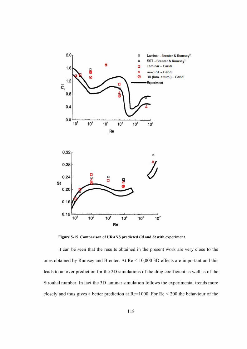
118
Figure 5-15 Comparison of URANS predicted Cd and St with experiment.
It can be seen that the results obtained in the present work are very close to the
ones obtained by Rumsey and Brenter. At Re < 10,000 3D effects are important and this
leads to an over prediction for the 2D simulations of the drag coefficient as well as of the
Strouhal number. In fact the 3D laminar simulation follows the experimental trends more
closely and thus gives a better prediction at Re=1000. For Re < 200 the behaviour of the

119
flow is almost 2D and the 2D simulations compare much better with experiments. Re =
89,000 is a very sensitive Reynolds number as it is close to the transition from the
subcritical to the supercritical regime. In this case we found out that the simulation is
very sensitive to the variation of the turbulence of the flow at the far field (i.e. inlet
turbulence boundary condition), [45]. It can be seen that the overall trends are well
captured.
Figure 5-16 Comparison of LES predicted Cd and St with experiment.

120
In Figure 5-16 LES simulation results are reported at Re = 3,900. Two cases were
run with 4 and 24 planes along the span (referred to as DPA in the Figure). Also results
from Young Ooi [45] are reported for comparison. It is evident that 4 planes are
insufficient and the drag and Strouhal number obtained are very close to 2D results.
While with 24 planes the agreement with experimental data is very good and much better
than the one obtained with URANS at similar Reynolds number.
Figure 5-17 Computed separation and transition over 2D cylinder by URANS simulation.
A study was performed to investigate the transition and the separation point for
the different flow regimes, i.e. at different Reynolds numbers. Because the separation and
transition are both unsteady phenomena, an average value for their position was
computed. Results for URANS are reported in Figure 5-17. This behavior is in agreement
with experimental evidence.

121
In the following Figure 5-18 the comparison between the computed and
experimental flow field is shown.
Figure 5-18 URANS flow field comparison.
The noise at a microphone placed at 128 diameters and at 90 degrees to the flow
direction was computed using the FW-H Acoustic Analogy. For 2D simulation a
correlation length must be specified as the contribution to the noise comes from all the
2D sections that makes up the real cylinder which is 3D, see Figure 5-19. Experimental
testing shows that the vortices are correlated, that is they fluctuate at the same frequency,
for a length that ranges from about 5 to 10 diameters.

122
Figure 5-19 Concept of correlation length.
A sensitivity analysis to the correlation length was performed and is reported in
the next Figure 5-20.
Figure 5-20 Correlation length sensitivity study.
It shows that the big change in the SPL occurs between 2 and 6 diameter length.
For the 2D computation a correlation length of 10 diameters was used as suggested in
[11].
Picco I Armonica, mic_2
20
30
40
50
60
70
80
90
100
110
120
2 4 6 8 10 12 14 16 18 20
Lungh. di Correlazione/D
SPL [dB]
128D

123
The SPL spectrum for the 2D URANS computation is reported in Figure 5-21. It
can be seen that the peak level is well captured, but noise coming from other frequencies
is missing. This is due to the RANS model used which is incapable of describing all of
the turbulence scales. The smallest scales are generally damped out and this can explain
some lack of agreement for higher Strouhal numbers. We must also consider that 2D
simulations force the behaviour of the fluid to be much more ordered as there is no third
dimension which can create instabilities and can add other noise frequencies. The shift in
the Strouhal number is the same reported in the aerodynamic computations, see Figure 5-
15. It must be considered that the experimental data from Revell et al. shows a Strouhal
number of 0.17 which is the lower limit for the data at Reynolds 89,000 of Figure 5-5.
Re 89000, mic_2
20
30
40
50
60
70
80
90
100
110
120
0 0.1 0.2 0.3 0.4 0.5 0.6 0.7
St
SPL [dB]Data - Revell et al.
kw-SST - Caridi
Figure 5-21 Comparison of predicted and measured sound pressure level, FLUENT 2D URANS simulation.

124
The results obtained are quite similar to the ones obtained by Rumsey and Brenter
[11], which are shown in Figure 5-22. In this figure the different turbulent models are
also compared.
Figure 5-22 Comparison of measured and predicted sound pressure level by Rumsey and Brenter, [11].

125
5.3 PROPELLER NOISE
Two main propellers were chosen for simulating propeller noise:
NASA SR2
NACA 4-(3)(08)-03
The choice was made because of the availability of aerodynamics, aeroacoustics
and geometry data. Before proceeding with aeroacoustic computations it was thought to
be necessary to calculate the loading on the propellers and to compare it with
experimental data. In fact if the blade loading is incorrectly predicted the computed noise
will also be erroneous.
5.3.1 Experiments
In the following sections the details of the experimental testing for the NASA
SR2 and NACA 4-(3)(08)-03 are reported.
5.3.1.1 NASA SR2
Aerodynamic test data for NASA SR2 propeller were taken from the NASA TM-
87054 report [28]. In this case a low speed wind tunnel performance test was completed
at the NASA Lewis Research Center as part of the NASA Advanced Turboprop Program
(1975-1985). The 62.2 cm (24.5 in) diameter 8 blade adjustable pitch model was tested at
Mach numbers typical of takeoff, initial climb out, and landing speeds (i.e. from 0.10 t o
0.34) in the NASA Lewis 10- by 10-Foot Supersonic Wind Tunnel. The attractiveness of
advanced turboprop propulsion results from its potential for very high propulsive
efficiency at cruise speeds up to Mach 0.8.

126
In Figure 5-23 the design parameters curves that were used to build up the CAD
model of the NASA SR2 are shown. The propeller configuration chosen was that with
41.7 degree blade angle at 75% of the radius ( ref =41.7 deg) for simulation at M=0.1
and 59.7 degree blade angle at M=0.34.
Figure 5-23 Variation of propeller design parameters with blade radius for the unswept SR-2 propeller.
Figure 5-24 shows the test facility and it can be seen that the propeller is mounted
on a spinner. No information was given about the propeller geometry in the report but it
was possible to design it by a careful analysis of some pictures.
Figure 5-25 shows the CAD model of the NASA SR2 with the spinner that was
considered axisymmetric in order to apply the periodic condition in the CFD simulation.

127
Figure 5-24 Test facility: close up of the propeller and a cutaway view of the strut-mounted Lewis propeller test rig.
Figure 5-25 CAD of the NASA SR2 propeller with the spinner.

128
The aerodynamics experimental data are shown in Figure 5-26 and 5-27, for
M=0.1 and M=0.34.
To understand these maps the following formulas are reported:
Advanced RationD
VJ REF
0
Trust Coefficient42
0 Dn
TCT
Power Coefficient 53
0 Dn
PCP
Efficiency P
Tnet C
CJ
P
TV 0
Figure 5-26 SR-2 propeller efficiency map at a Mach number of 0.10.

129
Figure 5-27 SR-2 propeller efficiency map at a Mach number of 0.34.
Noise data on the SR-2 model propeller were taken in the NASA Lewis Research
Center using a 8- by 6-Foot Wind Tunnel, [31]. The propeller was tested at a fixed blade
setting angle of 59 degrees for all the various tunnel axial Mach numbers. Data are
available for M = 0.6, 0.65, 0.7, 0.75, 0.8, 0.85, 0.9. A schematic diagram of the
experimental facility with the transducers is shown in Figure 5-28.

130
Figure 5-28 Experimental facility for noise measurements of SR2 propeller at Lewis Research Center Cleveland, Ohio.
5.3.1.2 NACA 4-(3)(08)-03
Tests for the aerodynamic characteristics of the NACA 4-(3)(08)-03 two-blade
propellers were conducted in the Langley 8-foot high-speed tunnel for blade angles
between 40° and 65° and through a Mach number range up to 0.925, [25]. In the present
work the configuration with the blade angle at 55° and M=0.45 was considered. The
facility is shown in Figure 5-29 while the aerodynamic experimental data are reported in
Figure 5-30.

131
Figure 5-29 Test apparatus for aerodynamic force measurements.
Noise data were not available for the test condition of M=0.45, but it was
considered useful to validate the numerical model for the prediction of aerodynamic
loading before proceeding to acoustics computations.
Figure 5-30 Thrust and Power Coefficient for NACA 4-(3)(08)-03, 55° blade angle.

132
Aeroacoustics data for the two, four and seven blade NACA 4-(3)(08)-03
propeller are available in the report NACA-TN-1354, [26], In this case the measurements
were made in an open field and the flow stream velocity is 0. The propeller has a
diameter of 4 feet. A 200-horsepower variable-speed electric motor was used to drive the
test propellers. The motor was rigidly mounted on an outdoor test stand, Figure 5-31.
Figure 5-31 Seven blade NACA 4-(3)(08)-03 propeller mounted on test stand.
A microphone was placed at ground level to ensure maximum pick-up of all
frequencies and was located at a point 30 feet from the propeller hub and at 15° angle
behind the plane of rotation, =105° (where is the angle from propeller axis of
rotation, 0 in front). This particular angular position was chosen because it is near the
value of for maximum sound pressures for the range of sound harmonics measured.

133
A survey of rakes to measure total pressure was clamped to the motor housing at
approximately 4 inches behind the propeller. The measured total pressure was integrated
over the disk area to obtain an estimate of total thrust. These measurements are believed
to be sufficiently accurate ( 25 %) for sound calculations. This error in thrust represents
approximately 1 decibel error in sound intensity.
Sound pressures and frequencies were measured with a Western Electric moving-
coil pressure-type microphone and a Hewlitt Packard Wave Analyzer. Data were
obtained at tip Mach numbers of 0.3, 0.5, 0.7 and 0.9. Gusts of wind cause a violent
fluctuation in sound pressures for all frequencies of the emitted noise. Measurements on
the seven-blade propeller at a 20° blade angle, taken on a day when gusts were
approximately 20 miles per hour, showed sound pressure variations of approximately 15
decibels at all speeds of the propeller. In order to obtain consistent data, testes were run
only on days when the wind velocities were low.
5.3.2 Simulation Set Up
Before simulating NASA SR2 and NACA 4-(3)(08)-03 propeller a thorough
investigation was carried out regarding the methods available in the FLUENT software
for the simulation of rotors [44]. In order to do this a simple rotor test was designed and
the fluid domain was generated with a tetrahedral mesh, Figure 5-32. This test case was
to define some methodologies for improving the iterative convergence and reducing the
CPU time of the simulation.

134
Figure 5-32 Rotor test for investigating the rotating object models.
The following studies were carried out:
Moving Reference Frame (MRF) vs. Sliding Mesh (SLM) approach
Periodic Boundary Condition testing
Convergence analysis
CPU time reduction
After these studies, it was clear that SLM model is much more expensive as it
requires transient simulation. Furthermore, in order to achieve the same results of MRF
very small time-steps and/or many sub-iterations are necessary. But if we are interested in
the evaluation of average value of the loading, the MRF model can represent a cheaper
alternative to the more expensive SLM, with about the same accuracy. The Periodic
Boundary Condition implemented in FLUENT works very well and can be utilised to
significantly reduce the dimension of the computational domain. For both MRF and SLM
models gradually increasing the rotational speed with a first order accurate solution was
found to be the best approach to reduce the computation time and avoid as possible
convergence problems.

135
Figure 5-33 Periodic domain for NASA SR2 propeller.
The periodic domain designed for NASA SR2 propeller is shown in Figure 5-33.
Two grids for SR2 model were generated with TGRID and tested:
2.2 million hybrid grid (5 prism layers + tetrahedral cells)
1.7 million polyhedral grid (generated from the hybrid one)
Some details of the grid are shown in Figure 5-34 and 5-35.

136
Figure 5-34 Surface and hybrid volume grid for SR2 propeller.
Figure 5-35 Detail of the 5 prism layers. Notice that the growth of the prism layers is takinginto account the curvature of the airfoil section.

137
The quality of the volume grid obtained was good with a maximum skewness of
0.85. Attention was paid to create a regular surface and volume mesh. The mesh
generation was automated by writing some scripts for TGRID. Hence, it was possible to
quickly change grid parameters, such as the growth rate of prism or volume mesh,
numbers of prism layers, constraints on orthogonality of prism layers to generate a
number of different grids. The best quality grid could then be chosen for CFD
simulations. In Figure 5-36 it is possible to see the surface polyhedral mesh generated as
conversion of the tetrahedral one.
Figure 5-36 Comparison of the surface mesh for tetrahedral and polyhedral grid.

138
For the NACA 4-(3)(08)-03 three domains were created, two similar to the SR2
(for 2 and 7 blade propeller), and one that was reproducing the experimental apparatus
used for aeroacoustic measurements, see Figures 5-37 and 5-38.
Figure 5-37 Computational domain for 7 and 2 blade NACA 4-(3)(08)-03 propeller.

139
Figure 5-38 Computational domain for 2 blade NACA 4-(3)(08)-03 propeller reproducing the experimental apparatus for aeroacoustic measurements.
Figure 5-38 shows the detail of the domain realized to reproduce the experimental
test facility used for the aeroacoustic test. It can be noticed the fluid volume surrounding
the propeller that will be used as rotational domain for Sliding Mesh simulation. The
ground was also modelled in this case.
Figure 5-39 Detail of 2 blade NACA 4-(3)(08)-03, CAD and surface mesh.

140
The mesh generated for the NACA 4-(3)(08)-03 propeller was a hybrid mesh
similar to that used for the NASA SR2 simulation. 5 prism layers were used and the final
mesh contained approximately 2.4 million cells for the 2 and 7 blade configurations in
free field. The mesh which included the experimental aeroacoustic apparatus required a
cell count of around 4.4 million. All the grids were generated with TGRID.
The height of the first prism layer was chosen in order to be able to use wall
function wall modelling available in FLUENT, 30<y+<150. In particular, non-
equilibrium wall functions were used, which have some correction terms to account for
pressure gradient effects.
The main settings used for the simulations are listed below:
• Pressure Based Coupled Solver
• II order implicit Unsteady formulation for transient SLM
• Discretization Scheme: PRESTO for Pressure, II order upwind for all the other
convective terms
• Viscous Model: k- realizable, non equilibrium wall function
• Green Gauss Node Based gradient discretization
• MRF or SLM model
Some incompressible simulations (e.g. M=0.1) were run with the segregated
solver because the coupling of pressure and velocity equations requires much more
computer RAM and sometimes 2 GB were not sufficient. Hence, the segregated or
coupled solvers were chosen depending on the hardware resources available. The
segregated solver should arrive at an identical result, but it can take many more iterations
to reach a converged solution.

141
As stated above, to accelerate the convergence and to avoid some convergence
problems, the rotational speed was gradually increased to the target value, starting with a
first order discretization scheme to improve stability.
5.3.3 Results
5.3.3.1 NASA SR2
Initial simulations were carried out to investigate the effect of the computational
grid on the results. In order to do this, results from tetrahedral and polyhedral grids were
compared. The number of prism layers utilised was also varied, but the results did not
show large differences. Hence, only results for grids containing 5 prism layers will be
reported here. In Figure 5-40 tetrahedral MRF simulation results in terms of aerodynamic
coefficients are compared to experimental data. Figure 5-41 shows the same results from
a simulation carried out with a polyhedral grid for comparison.
Figure 5-40 Predicted and measured aerodynamic coefficients of SR2 (tetrahedral grid).

142
Figure 5-41 Predicted and measured aerodynamic coefficients of SR2 (polyhedral grid).
In can be noticed that the thrust coefficient is always under-predicted, as well as
the power coefficient. The error in the computation of the efficiency increases with
advanced ratio. Because of these discrepancies encountered at the beginning of the study
on the tetrahedral grid a grid sensitivity analysis was carried out to see if the problems
could be attributed to the grid being used. The polyhedral grid investigated is quite
different in its topology and also changing the number of prism layers is a quite
significant change to the grid. But the results of the CFD simulations did not change on
these very different grids. It is noted that a more accurate solution could have been
achieved by running a simulation with a high quality hexahedral grid. It is known that
hexahedral elements are less numerically dissipative and thus results can be more
accurate when they are utilised. Other numerical modelling effects were also investigated
without changing the grid, by reducing the viscosity of the simulation, changing
turbulence modelling, and eliminating turbulence effects completely by carrying out a

143
laminar simulation. Furthermore, an inviscid simulation was performed which is an even
more extreme case. The effect of viscosity on the aerodynamic coefficients is shown in
Figure 5-42.
Figure 5-42 The effect of viscosity on the aerodynamic coefficients.
It can be seen that even with an extreme inviscid simulation the thrust is strongly
under-estimated as is the aerodynamic power. This may be expected as the thrust depends
mainly on the lift generated by the airfoils, which is not very much affected by the
viscosity when the flow is not separated on the airfoil sections (as it was verified to be
attached). It is clear that decreasing the fluid viscosity reduces the power which is also
related to the viscous losses that the propeller experiences in its rotation (P=M). These
two effects generate the increase in propeller efficiency.

144
It was thought that maybe the thrust and power discrepancies could be caused by
a blade angle defect, as may be expected when comparing a simulation which is in an
ideal free field with experimental data measured in a real-world wind tunnel. The
efficiency errors may be due to an overly dissipative numerical solution of the flow field.
For this reason, a blade angle analysis was carried out, Figure 5-43.
Figure 5-43 Blade angle analysis: computed coefficients at 41.7° are compared to experimental data at 40° blade angle.
The blade angle analysis involved carrying out a simulation at a blade angle of
41.7°. The results of this simulation were found to better match the thrust and power
curves for experimental data at 40°. However, an inconsistency was also discovered: the
efficiency correlation is actually worse in this case, even for the inviscid simulation.
Hence, some doubts about the geometry construction and about how the experimental

145
measurements were taken arose. Unknown factors in the experimental measurements
may be unaccounted for in the CFD analysis. These issues may be caused by a
combination of effects: geometry (which was built from tables), experimental data and
maybe some inaccuracy in the simulation, in particular at higher advanced ratio, when the
absolute values of the forces are smaller and are thus more prone to numerical error. This
last error could be reduced by a high quality hexahedral mesh and using less dissipative
higher order schemes available in FLUENT (although it was shown that even with an
inviscid simulation the agreement with experiments was not improved). Because of these
highly relevant discrepancies with the loading computation, further aeroacoustic
simulations were not performed. It was decided to work on the NACA 4-(3)(08)-03
propeller which, as we will see shortly, gave much better results for aerodynamic force
predictions. Although aeroacoustic analysis was not carried out, the aerodynamic
simulations still gave a deep insight into the flow mechanics of the propeller, see Figure
5-44.
Figure 5-44 Tip vortices detail of the flow field of SR2 propeller.

146
5.3.3.2 NACA 4-(3)(08)-03
In the Figure 5-45, aerodynamic coefficients computed with the MRF model at
M=0.45, 55° blade angle are compared with experimental data. The simulations included
compressibility effects, increasing the physical complexity from those carried out on
the NASA SR2. This made numerical convergence of the simulations more
problematic.
Figure 5-45 Predicted and measured aerodynamic coefficients of NACA 4-(3)(08)-03.
The agreement in this case is very good indeed, for all the curves. At higher
advanced ratio the computed efficiency curve start bending before the experimental one.
As mentioned above, at higher advanced ratio the forces are smaller and numerical errors
may become more significant. As the aerodynamics simulations were in good agreement
with experimental data, it was decided to continue with an investigation into the

147
aeroacoustics. When the simulation is steady as in the MRF it is possible to use the
steady state formulation of the Ffowcs-Williams and Hawkings Acoustic Analogy: the
Gutin model, available in FLUENT 6.3.23. This is very important because the CPU time
can be reduced by almost one order of magnitude from that required for the unsteady
formulation.
Figure 5-46 Predicted and measured thrust for NACA 4-(3)(08)-03 at M=0.
When the flow direction is not aligned with the axis of rotation it is not possible to
use the Gutin model because the loading on the blade is unsteady, so a transient SLM
simulation should be performed and the full Ffowcs-Williams and Hawkings Analogy
Naca 7 pale 16.5 deg - punto fisso
-100
0
100
200
300
400
500
600
0 500 1000 1500 2000 2500 3000 3500 4000
rpm
Tru
st
lb
Exp. Lower Limit
Fluent - Free Field
Exp. Upper Limit
Poli. (Fluent - Free Field)
Poli. (Exp. Lower Limit)
Poli. (Exp. Upper Limit)
Naca 2 pale 16.5 deg - punto fisso
-50
0
50
100
150
200
250
300
350
400
450
0 1000 2000 3000 4000 5000 6000
rpm
Tru
st
lb
Exp. Lower Limit
Fluent - Free Field
Exp. Upper Limit
Poli. (Fluent - Free Field)
Poli. (Exp. Lower Limit)
Poli. (Exp. Upper Limit)

148
should be used. The results for the acoustic simulations were first compared in terms of
aerodynamic forces.
Figure 5-47 shows the comparison between the computed and experimental thrust
for 2 and 7 blade NACA 4-(3)(08)-03 at M=0, 16.5 blade angle as in the aeroacoustic
experiments. Simulated results match with the upper limit experimental thrust curve.
After this aerodynamic analysis, noise was computed for different configurations:
For 2 blade propeller: periodic MRF simulation in free field
For 7 blade propeller: periodic MRF simulation in free field, unsteady
periodic SLM simulation only at 1600 rpm
2 blades simulation with ground and test stand: unsteady SLM simulation
An example of the acoustics analysis is shown in Figure 5-45: both with Gutin or
full FW-H analogy time pressure history is recorded at the microphone location and then
the signal is Fourier transformed in the frequency domain.
Figure 5-47 Acoustic data post-processing.
Aeroacoustics results for 2 blade propeller are reported in Figure 5-48. The
comparison is made at 1600, 2680, 3770, 4850 rpm. For a better understanding of the
results it is necessary to explain and detail the legend:

149
OSPL: Overall Sound Pressure Level
OSPL FLU: OSPL FLUENT - Steady CFD Moving Reference Frame
with Gutin Aeroacoustic Model
OSPL FLU mod. GUTIN: OSPL computed with an other Gutin formula
[26] with blade loads computed by FLUENT
Exp. Wave A. Mic.: Experimental data OSPL processed with Wave
Analyzer (only blade Frequencies and Harmonics are taken into account)
Exp. Volt. Mic.: Experimental data OSPL
OSPL FLU GROUND SLM: OSPL FLUENT - Unsteady CFD Sliding
Mesh with FW-H, with ground and test stand
Figure 5-48 Predicted and measured SPL for 2 blade NACA 4-(3)(08)-03 at M=0.
Naca 2 Blades 16.5 deg. M=0
646668707274767880828486889092949698
100102104106108110112114116118120122124126128
1600 2680 3770 4850
rpm
dB
OSPL FLU
OSPL FLU mod. GUTIN
Exp. Wave A. Mic.
Exp. Volt. Mic.
OSPL FLU GROUND SLM

150
Very good agreement with experimental measurements is obtained at 2680, 3770
and 4850 rpm. The difference with experiments is maximum 1-3 dB for both the
computed methods used: directly with FLUENT (referred to as OSPL FLU) and using
Gutin formula [26] with the aerodynamic loads computed with FLUENT (referred to as
OSPL FLU mod. GUTIN). It is quite evident the under-prediction at low rotational speed.
To understand better these discrepancies we have to point out which is the
difference between the two methods used to measure the propeller noise: classic
microphone-voltmeter (referred to Exp. Volt. Mic.) and wave-analyzer processed data
(referred to as Exp. Wave A. Mic.).
In the first case the measured total microphone voltage is converted directly to
decibels. This gives the summation of the entire band of frequencies emitted. When
measurements are filtered by wave-analyzer only the sound pressure corresponding to the
rotational noise-frequency peaks are summed (the first 5 harmonics).
Therefore, if the vortex noise is strong compared with the rotational noise, as it is
usually the case at low tip Mach numbers, values determined by microphone voltage will
be larger than values determined from wave-analyzer measurements [26].
So it seems that with a steady MRF simulation the Gutin model it is not possible
to predict vortex noise at low rotational speed. For this reason, an unsteady Sliding Mesh
simulation was also performed at 1600 rpm (referred to as OSPL FLU GROUND SLM in
Figure 5-48) with the ground and the test stand. The sound pressure level computed was
76.5 which was 2 dB higher than the MRF free field simulation, but still under predicting
microphone-voltmeter experimental data. It is thought that it is more appropriate to
compare aeroacoustic computations with the wave-analyzer measurements. This is

151
because by using URANS turbulence models we do not detect most of the contribution
from all the band of frequencies, in particular broadband noise which is indeed measured
by the voltage microphone. Generally by using URANS we catch only the first harmonics
peaks. So if we compare to the wave-analyzer measurements we have 76.5 dB level
against experimental 79 dB. Similar considerations can be done for the 7 blade propeller
configuration shown in Figure 5-49. The agreement between steady periodic MRF
simulation and experiment is very good at 3450 rpm and 2680 rpm but it is again much
worse at the lower rotational speed of 1600 rpm. It can be seen that the difference
between the two methods of experimental measurement is very large at 1600 rpm for the
7 blade propeller. This suggests that vortex noise weighs more compared to rotational
noise in the case of a 7 blade configuration compared to a 2 blade one.
Naca 7 Blades 16.5 deg. M=0
38404244464850525456586062646668707274767880828486889092949698
100102104
1600 2680 3450
rpm
dB
OSPL FLU
OSPL FLU mod. GUTIN
Exp. Wave A. Mic.
Exp. Volt. Mic.
OSPL FLU SLM NO GROUND
Figure 5-49 Predicted and measured SPL for 7 blade NACA 4-(3)(08)-03 at M=0.

152
With an unsteady SLM simulation (referred to as OSPL FLU SLM NO GROUND
in Figure 5-49, because it is in free field without ground and test stand) the computed
results were improved from 42.5 dB to 54 dB, but wave-analyzer is still in poor
agreement at approximately 68 dB. The reason for not performing a simulation including
the ground and test stand is that, for the 7 blade configuration, the mesh size would have
increased to 14 million cells. This is far too computationally expensive for running a
transient SLM simulation. An MRF simulation in free field was simulated using periodic
boundary conditions such that only one-seventh of the domain could be considered. In
order to match the experimental data at 1600 rpm, it is suggested that a much more
accurate simulation is needed to be able to catch all the transient features and broadband
noise (smaller timestep, DES or LES turbulence model, hexahedral grid).
Figure 5-50 shows a detail of the tip vortices of the SLM simulation with test
stand and ground.
Figure 5-50 Flow field detail showing the tip vortices of the NACA 4-(3)(08)-03 at M=0,
simulated with SLM model and reproducing the ground test facility for noise measurements.

153
5.4 JET NOISE
In the following sections the simulation of a heated jet by 2D URANS and 3D
LES modelling and the comparison with laboratory experiments will be described. In this
case, for noise computation, FW-H analogy with porous surface is the right choice
because using CAA is not practical as the microphones are placed quite away, no big
obstacles are presents between the source and the receiver, furthermore no physical
surfaces are present and the phenomenon is due to the free turbulence of the jet.
5.4.1 Experiments
The experiment was performed in the Small Hot Jet Acoustic Rig in the
Aeroacoustics Propulsion Laboratory (AAPL) of NASA Glenn Research Center. AAPL
is a 65 ft (20 m) radius, anechoic, geodesic-dome. The walls of the dome and
approximately half of the floor area are treated with acoustic wedges made from
fibreglass wool to render the facility anechoic above 220 Hz. A 60 in. (1.5 m) exhaust fan
in the top of the dome provides air circulation. Flows from all rigs are directed out the 55
ft (16.8 m) wide by 35 ft (10.7 m) high doorway to an open field (Castner 1994). The jet
facility is capable of producing heated jets with total temperature from ambient to 920 K
in the Mach number range 0 < M < 2, and therefore ideal for studying the effect of
heating. A 2 in. (50.8 mm) diameter convergent nozzle was used for all measurement
conditions. Among the all tested conditions it was simulated the case at Ma=0.9, TR=2.7.

154
Figure 5-51 Operating conditions of the tested jet.
Here Ma is the commonly used parameter for sound radiation (that involves
coupling between jet velocity, referred to as Uj in Figure 5-51, and ambient sound speed,
referred to as a0), the compressibility effect is represented by the jet Mach number
Mj= Uj/ aj, TR=Tj/Ta is the jet static temperature ratio, where aj is the speed of sound and
Tj the temperature in the jet core.
The far field sound pressure fluctuations were measured by an array of seven ¼
in. (6.35mm) microphones kept on an arc of 100 D (5.08 m) and centred at the nozzle
exit. The microphones were angularly placed with 10° increments: from 150° to 90° to
the jet exit (Figure 5-52). Polar angles were measured from the flight direction (opposite
to the jet direction). The presence of the large traversing unit, optical components and
other metal surfaces was a concern for significant acoustic reflection. To minimize such
reflection a large part of such surfaces were covered by 50 mm thick polyurethane foams.
Figures 5-52, 53 show some details of the experimental apparatus.

155
Figure 5-52 Photograph showing side view of the Small Hot Jet Acoustic Rig, X-Y traverse holdingthe Rayleigh setup, and microphones.
Figure 5-53 Photograph showing the front view of the jet facility and the Rayleigh setup.

156
Figure 5-54 Far field, narrowband, microphone spectra from indicated polar angles obtained from fixed Ma = 0.9 jets at indicated temperature ratios. (c) and (d) show the same data in (a) and (b) but normalized by a different factor. All microphones were positioned on a 100 diameters arc (diameter=2 inches).
The effect of heating on the far field noise spectra of a fixed velocity (Ma = 0.9) is
shown in Figure 5-54. The narrowband spectra were obtained from power spectra
calculations of the microphone time signals. The frequency values were converted to
Strouhal number St = fD/Uj (f is frequency), and the power spectra Sp’2 were converted
into spectral density per unit Strouhal frequency Sp’2/ (Δf D/ Uj), where Δf is the width of
each frequency bin. Interestingly, Figure 5-54 (a) shows that in the shallow angle the low
frequency part 0≤ St ≤0.5 remains nearly unchanged with increasing plume temperature,
while the higher frequency part continually decreases. For the 100° location, heating
causes progressive lowering of sound emission at all frequencies. The increase in the jet
temperature is expected to reduce high frequency radiation from the shallow angles due
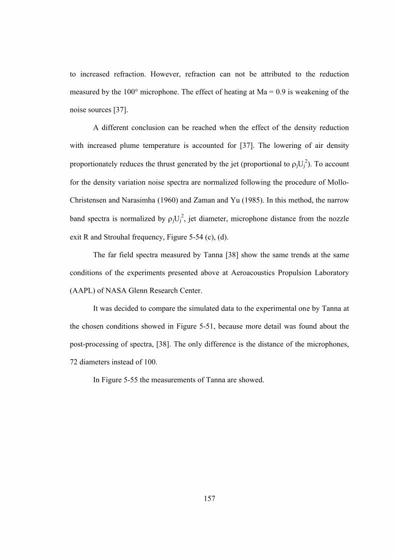
157
to increased refraction. However, refraction can not be attributed to the reduction
measured by the 100° microphone. The effect of heating at Ma = 0.9 is weakening of the
noise sources [37].
A different conclusion can be reached when the effect of the density reduction
with increased plume temperature is accounted for [37]. The lowering of air density
proportionately reduces the thrust generated by the jet (proportional to jUj2). To account
for the density variation noise spectra are normalized following the procedure of Mollo-
Christensen and Narasimha (1960) and Zaman and Yu (1985). In this method, the narrow
band spectra is normalized by jUj2, jet diameter, microphone distance from the nozzle
exit R and Strouhal frequency, Figure 5-54 (c), (d).
The far field spectra measured by Tanna [38] show the same trends at the same
conditions of the experiments presented above at Aeroacoustics Propulsion Laboratory
(AAPL) of NASA Glenn Research Center.
It was decided to compare the simulated data to the experimental one by Tanna at
the chosen conditions showed in Figure 5-51, because more detail was found about the
post-processing of spectra, [38]. The only difference is the distance of the microphones,
72 diameters instead of 100.
In Figure 5-55 the measurements of Tanna are showed.

158
Figure 5-55 Far field noise spectra from jets produced by 2 inches diameter nozzle at different Ma and TR. Columns (a), (b), and (c) presents data at Ma = 0.6, 0.9, and 1.48 respectively; rows (1), (2), and (3) are from different microphone angles θ = 150°, 90°, and 60° respectively. All microphones were positioned on a 72 diameters arc. All data are from a convergent nozzle except for a convergent-divergent nozzle for the unheated Ma = 1.48 jet.Measurements by Tanna, [38].
5.4.2 Simulation Set Up
Before proceeding to simulate the 3D case, it was decided to tune the
methodology using a 2D URANS axisymmetric simulation. The aims of the 2D
simulation were to design the dimension of the domain, to verify the boundary conditions
used and to find a suitable position for the porous surface (referred to also as permeable
surface) where pressure fluctuations are recorded for the Acoustic Analogy. The 2D grid
is then used to create the 3D grid.

159
In the following Figure 5-56 the 2D domain is shown along with the boundary
conditions used. Figure 5-57 shows the details around the nozzle exit area..
Figure 5-56 Computational 2D axisymmetrical domain with boundary conditions used.
Figure 5-57 Detail at the nozzle exit and of the FW-H porous surface.
A large domain was utilized for the following reasons:
• To eliminate spurious reflections when not using Non Reflective Boundary
Condition (NRBC are available only for Density Based Solver with some
limitations, and not for PBCS)
• To allow large cells at the far-field to act as a numerical filter damping high
frequency pressure wave
• To eliminate reversed flow at the boundaries. To obtain this it was also added a
low mass flow inlet (about 4 m/s) at the inlet boundary, far from the shear layer.
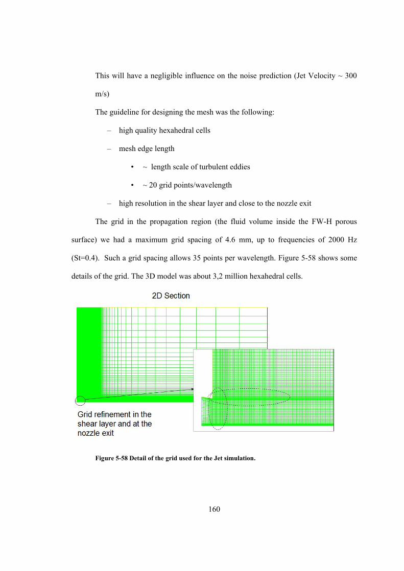
160
This will have a negligible influence on the noise prediction (Jet Velocity ~ 300
m/s)
The guideline for designing the mesh was the following:
– high quality hexahedral cells
– mesh edge length
• ~ length scale of turbulent eddies
• ~ 20 grid points/wavelength
– high resolution in the shear layer and close to the nozzle exit
The grid in the propagation region (the fluid volume inside the FW-H porous
surface) we had a maximum grid spacing of 4.6 mm, up to frequencies of 2000 Hz
(St=0.4). Such a grid spacing allows 35 points per wavelength. Figure 5-58 shows some
details of the grid. The 3D model was about 3,2 million hexahedral cells.
Figure 5-58 Detail of the grid used for the Jet simulation.

161
Figure 5-59 Detail of the grid used for the Jet simulation.
The FW-H porous surface position was set based upon results from the 2D
simulation according to the following requirements:
• must enclose all the main aeroacoustic sources of interest
• must be as small as possible because inside sound propagation must be computed
(CAA) and for longer paths more sound will be dissipated
• must not cross high vorticity and non linear regions (in this case it was left open at
the bottom)
Figure 5-60 shows the results of the 2D simulation verifying the position of the
FW-H porous surface. Areas of high vorticity can be seen to lie within the FW-H surface.

162
Figure 5-60 Vorticity Magnitude for the 2D axisymmetric simulation.
Figure 5-61 shows the contour plot of the acoustic power using the Proudman’s
formula [46]. This gives an indication about the quadrupole source strength; areas of high
acoustic power are all inside the FW-H permeable surface.
Figure 5-61 Contour of Acoustic Power calculated by Proudman’s formula, 2D axisymmetric simulation.

163
The timestep was set to 1e-05 s, which guarantees more than 30 points in the
period corresponding to the signal of 2000 Hz. Cell Courant number was <1 in almost all
the domain as shown in Figure 5-62 for the 3D LES simulation.
Figure 5-62 Histogram of cell Courant number for 3D LES simulation, 99% of the cells in the domain have a value<1.
The main settings used for the simulations are listed below:
• Double Precision Pressure Based Coupled Solver
• Ideal gas law for air density
• II Order implicit unsteady formulation
• Discretization: III order QUICK for URANS simulation, Bounded Central
Differencing for LES
• Viscosity: Sutherland Model
• Thermal Conductivity: Kinetic Theory Model
• Viscous model: k-ω standard for URANS, Lilly-Smagorinsky for LES
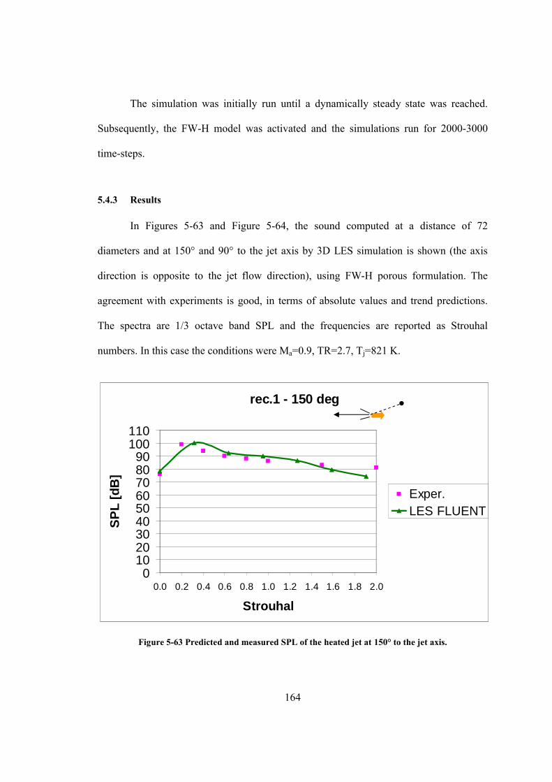
164
The simulation was initially run until a dynamically steady state was reached.
Subsequently, the FW-H model was activated and the simulations run for 2000-3000
time-steps.
5.4.3 Results
In Figures 5-63 and Figure 5-64, the sound computed at a distance of 72
diameters and at 150° and 90° to the jet axis by 3D LES simulation is shown (the axis
direction is opposite to the jet flow direction), using FW-H porous formulation. The
agreement with experiments is good, in terms of absolute values and trend predictions.
The spectra are 1/3 octave band SPL and the frequencies are reported as Strouhal
numbers. In this case the conditions were Ma=0.9, TR=2.7, Tj=821 K.
Figure 5-63 Predicted and measured SPL of the heated jet at 150° to the jet axis.
rec.1 - 150 deg
0102030405060708090
100110
0.0 0.2 0.4 0.6 0.8 1.0 1.2 1.4 1.6 1.8 2.0
Strouhal
SP
L [
dB
]
Exper.LES FLUENT

165
Figure 5-63 shows that at 150° the SPL peak is predicted at a slightly higher
frequency than the experimental measurement. In Figure 5-64 it is shown that at 90°, the
reduction of SPL (relative to that calculated at 150°) is well captured, as is the lesser
gradient of the curve.
As outlined in the previous section regarding the design of the grid and of the
time-step size, the results should be considered reliable up to a Strouhal number of about
1 (10-15 points per wavelength for a signal of 6000 Hz St=0.95).
rec.7 - 90 deg
0102030405060708090
100110
0.0 0.2 0.4 0.6 0.8 1.0 1.2 1.4 1.6 1.8 2.0
Strouhal
SP
L [
dB
]
Exper.
LES FLUENT
Figure 5-64 Predicted and measured SPL of the heated jet at 90° to the jet axis.
LES simulations can give a great insight into the physics of the heated jet. In
Figure 5-65 and 5-66 the instantaneous velocity magnitude contour as well as the time–
averaged velocity magnitude contour over a long duration are shown.
It is interesting to notice that the potential core is well distinguishable only in the
time averaged image, see Figure 5-66.
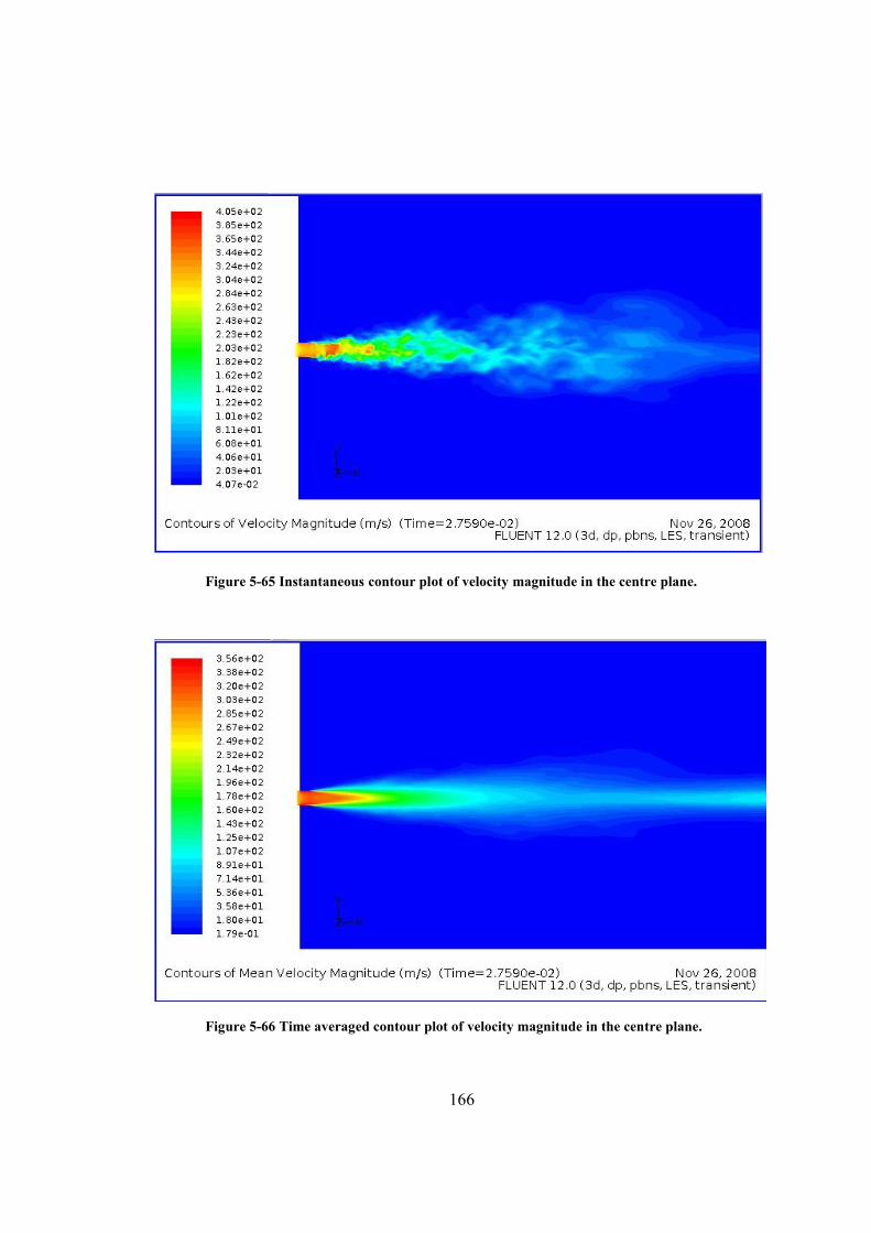
166
Figure 5-65 Instantaneous contour plot of velocity magnitude in the centre plane.
Figure 5-66 Time averaged contour plot of velocity magnitude in the centre plane.

167
Figure 5-67 Instantaneous contour plot of static temperature in the centre plane.
Figure 5-68 Instantaneous contour plot of air density in the centre plane.

168
Figure 5-67 and 5-68 show instantaneous contours of the static temperature and
air density through the centre of the jet. It is clear that all the mixing happens in the shear
layer, which is appropriately named the mixing region. In Figure 5-69 the Root Mean
Square (RMS) of the static temperature shows where the main unsteadiness of
temperature occurs. It is evident that the potential core is very stable as it experiences
almost negligible fluctuations.
Figure 5-69 RMS contour plot of static temperature fluctuations in the centre plane.
High vorticity regions are visible around the end of the potential core and few
diameters downstream, see Figure 5-70. As this is also the area that experiences the main
unsteadiness in pressure, see Figure 5-71, it may be considered a region of strong noise
sources according to the theory presented in Chapter IV.
Figure 5-72 gives an insight into the turbulent length scale structure of the jet. Iso-
surfaces, using the Q-criterion (Hunt, Wray & Moin, 1988) are coloured by static

169
temperature. The smaller scales near the potential core and the bigger scales further
downstream are clearly visible.
Figure 5-70 Instantaneous contour plot of vorticity magnitude in the centre plane.
Figure 5-71 Contour plot of RMS static pressure fluctuations in the centre plane.

170
Figure 5-72 Iso-surfaces created by applying the Q-criterion, colored by static temperature.

171
6 CONCLUSION
Methodologies for simulating different types of aerodynamically generated noise
have been developed herein. Limitations in these methods have been highlighted and
suggestions have been made for the optimum approach to simulate each type of noise
considered. In order to do this, an entire Chapter of this study is dedicated to the
understanding of noise generation mechanisms. Such an understanding is fundamental to
ensure the simulation is set up correctly and to properly analyze the results. Engineers
today can often be too hasty to simulate almost everything by CFD, without first
deepening their understanding of the fundamental physical phenomena which they look
to investigate. This generally leads to poor results and the impossibility to understand
which step to subsequently take in order to improve their results. Today, this is
particularly true in the area of aeroacoustics, which still represents a promising but
challenging area of research in the industrial environment.
The investigation into cavity noise showed how it is possible to predict the
fundamental physics of buffeting with a “cheap” CAA 2D, compressible URANS
simulation. Results were presented which illustrated the ability of such a simulation to
predict the frequency of the coupled system, as well as the noise. Particular attention has
been paid to the construction of the computational grid and simulation procedure used. It
was shown how important the prediction of the boundary layer thickness at the leading

172
edge of the cavity is, as this affects the convective velocities of the shed vortices and thus
the frequency of buffeting. Comparisons with experiments and with other CFD
simulations from an important Aeroacoustic Benchmark [36] were reported. The
computational cost was considered “cheap” because the simulation time, on a modern
dual or quad core PC, would be around 2 days. This gives the possibility to use such a
simulation method as a tool to compare many different design configurations in order to
improve the acoustic performance, e.g. automotive door gaps. Recommendations for
future work on this subject would be to focus on computationally expensive 3D
simulations using LES or Detached Eddy Simulation (DES) turbulence models, to enable
the prediction of not just the tonal peak but also some broadband components.
The vortex shedding noise caused by fluid flow over cylinders has been
thoroughly investigated. Acoustic computations made use of the FW-H acoustic analogy.
The locations of the main sources of noise were found and used to choose optimal
positioning for the FW-H integration surface. The limitations of 2D URANS simulations
were highlighted which could be overcome by more detailed 3D LES simulations.
Unfortunately, it was not possible to run high Reynolds number simulations for
aeroacoustic comparison as they would be too computationally expensive to be run on the
hardware available (dual or quad core PCs). Such simulations would require a large
cluster of PCs for parallel CFD computations. A 3D LES simulation was run at a
Reynolds number of 3,900, showing very good improvement in both drag and Strouhal
number prediction. A study was also detailed on how to size a LES computational grid by
post-processing a cheaper RANS simulation. As expected boundary layer separation and
transition were shown to be highly dependent on the Reynolds number of the flow. These

173
phenomena strongly affect the vortex shedding and the emitted noise, and they were seen
to be accurately captured by the use of the k- SST transitional-flow turbulence model.
Comparison with unsteady aerodynamics and noise measurements were shown.
An extensive study was dedicated to propeller noise simulation. The investigation
began with aerodynamic simulations of propellers. A deep exploration into the
computational methods available for simulating rotors was carried out using moving
reference frames, sliding meshes and periodic modeling approaches.
After the analysis of the noise source type and location, two main methods were
investigated and compared: Steady (Gutin) and Unsteady formulation of FW-H analogy,
both with solid surface of integration. The first method is very efficient as it can be used
with a 3D periodic RANS simulation, while the latter requires a more expensive unsteady
simulation such as a periodic or non-periodic sliding mesh approach. Comparison with
experiments were performed for two and four blade NACA propellers at different
rotational speeds, using the different methods explained above. Good agreement was
found with the most inexpensive computational approach, i.e. the 3D RANS simulation
with the Gutin model, at medium and higher rotational speeds (errors were around 1-2
dB). At lower rotational speeds, the vortex noise component was not well predicted by
the steady state approach with the Gutin model. For this reason, a sliding mesh URANS
simulation which accurately reproduced the experimental facility using the full FW-H
analogy was performed. These simulations improved the results considerably but they
were still in poor agreement with the experimental data. It is thought that a much more
expensive and accurate unsteady simulation would be needed to improve upon these
results. Steady-state simulations are relatively inexpensive, requiring 1 day on a modern

174
quad core PC, while unsteady sliding mesh simulations required use of a 16 processor PC
cluster for about 3-4 CPU days. Although this is considered computationally expensive, it
is still affordable within an industrial environment. Such a sliding mesh approach is the
only one available to guarantee the accurate analysis of a complex configuration such as a
wing installed aircraft propeller. Future work on propeller aeroacoustics will be continued
as today there is a strong interest in this field.
Another important aeroacoustics problem encountered in aeronautical engineering
was studied here: the jet noise. The noise emitted by the exhaust plume from a gas
turbine engine continues to be a significant contributor to the total sound radiated from
current commercial airplanes. This is expected to be a bigger problem for future
commercial supersonic flights with lower bypass ratio engines. A methodology was
developed for predicting this phenomenon. In this case, due to the fact that the sound
receivers are positioned quite far from the jet and no large obstacles are present in the
domain, the FW-H analogy is the best choice of acoustics model. In this case, the
permeable formulation should be applied as no solid surfaces are present, and because the
noise sources are all due to the turbulence inside the jet. The Mach number of the jet
investigated here was 0.9.
It was suggested to first perform a 2D URANS axisymmetric simulation to verify
where to position the FW-H permeable surface. Guidelines were given for designing the
fluid domain and the computational grid. In this case, the acoustic analogy was applied,
but inside the FW-H surface a full CAA simulation was carried out in order to capture the
transmission of all the acoustic pressure fluctuations up to the permeable surface.

175
An accurate compressible LES simulation was performed, and results compared
to measurements. It can be seen that the agreement is satisfactory in terms of trends and
absolute values for both the microphones at 150° and 90° to the jet axis. The absolute
computed SPL values for the 150° microphone are within a few dB up to a Strouhal
number of about 1. A small shift is observed in the SPL peak compared to experimental
values. Results at 90° are slightly over-predicted, but the overall trends are predicted very
well. Post-processing of the simulation data has clearly shown the fundamental physics of
the jet, highlighting the potential core, the mixing region and the area of major noise
sources. A Q-criterion iso-surface visualization illustrated the turbulent length scale
structure of the jet in great detail. This simulation was run on a 16 processor PC cluster
for about 5-6 days. It was shown that the information gained by this LES simulation
could not have been realized using a cheaper URANS simulation.

176
References
[1] Lighthill, M. J., “On Sound Generated Aerodynamically, I. General Theory”,
Proceedings of the Royal Society of London, Vol. A211, No 1107, pp. 564-587,
1952.
[2] Lighthill, M. J., “On Sound Generated Aerodynamically, II. Turbulence as a source
of sound”, Proceedings of the Royal Society of London, Vol. A222, No 11048,
pp. 1-32, 1954.
[3] Curle, N., “The Influence of Solid Boundaries upon Aerodynamic Sound”,
Proceedings of the Royal Society of London, Vol. A231, pp. 505-514, 1955.
[4] Crighton, D.G., “Basic principles of aerodynamic noise generation”, Prog.
Aerospace Sci., 16:31-96, 1975.
[5] Howe, M.S., “Theory of Vortex Sound”, Cambridge University Press, 2003.
[6] J.E. Ffowcs Williams, D.L. Hawkings, “Sound generated by turbulence and surfaces
in arbitrary motion”, Philosophical Transaction of the Royal Society, A 264, No
1151, pp. 321-342, 1969.
[7] Colonius, T., Lele, S.K., “Computational aeroacoustics: progress on non linear
problems of sound generation”, Progress in Aeorspace Sciences, Vol. 40, pp. 345-
416, 2004.
[8] Brentner, K.S., Farassat, F., “An Analytical Comparison of the Acoustic Analogy
and Kirchhoff Formulations for Moving Surfaces”, AIAA Journal, Vol. 36, pp.
1379-1386, 1998.
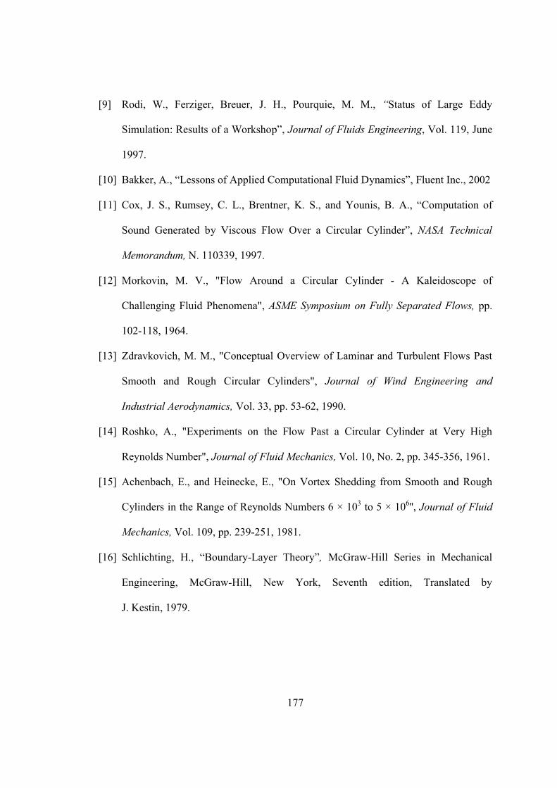
177
[9] Rodi, W., Ferziger, Breuer, J. H., Pourquie, M. M., “Status of Large Eddy
Simulation: Results of a Workshop”, Journal of Fluids Engineering, Vol. 119, June
1997.
[10] Bakker, A., “Lessons of Applied Computational Fluid Dynamics”, Fluent Inc., 2002
[11] Cox, J. S., Rumsey, C. L., Brentner, K. S., and Younis, B. A., “Computation of
Sound Generated by Viscous Flow Over a Circular Cylinder”, NASA Technical
Memorandum, N. 110339, 1997.
[12] Morkovin, M. V., "Flow Around a Circular Cylinder - A Kaleidoscope of
Challenging Fluid Phenomena", ASME Symposium on Fully Separated Flows, pp.
102-118, 1964.
[13] Zdravkovich, M. M., "Conceptual Overview of Laminar and Turbulent Flows Past
Smooth and Rough Circular Cylinders", Journal of Wind Engineering and
Industrial Aerodynamics, Vol. 33, pp. 53-62, 1990.
[14] Roshko, A., "Experiments on the Flow Past a Circular Cylinder at Very High
Reynolds Number", Journal of Fluid Mechanics, Vol. 10, No. 2, pp. 345-356, 1961.
[15] Achenbach, E., and Heinecke, E., "On Vortex Shedding from Smooth and Rough
Cylinders in the Range of Reynolds Numbers 6 × 10³ to 5 × 10⁶'', Journal of Fluid
Mechanics, Vol. 109, pp. 239-251, 1981.
[16] Schlichting, H., “Boundary-Layer Theory”, McGraw-Hill Series in Mechanical
Engineering, McGraw-Hill, New York, Seventh edition, Translated by
J. Kestin, 1979.

178
[17] Blackburn, H. M., and Melbourne, W. H., "The Effect of Free-Stream Turbulence
on Sectional Lift Forces on a Circular Cylinder", Journal of Fluid Mechanics, Vol.
306, pp. 267-292, 1996.
[18] Alemdaroglu, N., Rebillat, J. C., and Goethals, R., "An Aeroacoustic Coherence
Function Method Applied to Circular Cylinder Flows", Journal of Sound and
Vibration, Vol. 69, No. 3 , pp. 427-439, 1980.
[19] Mittal, R., and Balachandar, S., "Effect of Three-Dimensionality on the Lift and
Drag of Nominally Two-Dimensional Cylinders", Physics of Fluids, Vol. 7, No. 8,
pp. 1841-1865, Aug. 1995.
[20] Belov, A., Jameson, A., and Martinelli, L., "Three-Dimensional Unsteady
Incompressible Flow Calculations Using Multigrid", AIAA paper 97-0443, Jail.
1997.
[21] Franke, R., Rodi, W., and Schonung, B., "Numerical Calculation of Laminar
Vortex-Shedding Flow Past Cylinders", Journal of Wind Engineering and Industrial
Aerodynamics, Vol. 35, pp. 237-257, 1990.
[22] Revell, J. D., Prydz, R. A., and Hays, A. P., "Experimental Study of Airframe Noise
vs. Drag Relationship for Circular Cylinders", Lockheed Report, No. 28074, Final
Report for NASA Contract NAS1-14403, Feb. 1977.
[23] “Aeroacoustics of Flight Vehicles: Theory and Practice”, NASA Reference
Publication, No. 1258, Vol. 1 WRDC Technical Report 90-3052, 1991.
[24] Brooks, T. F., Pope, D. S., and Marcolini, M. A, “Airfoil Self-Noise and
Prediction”, NASA Reference Publication, No. 1218, 1989.

179
[25] Camel, M. M., Morgan, F. G. Jr., and Coppolino D. A. “Effect of Compressibility
and Camber as Determined from an Investigation of the NACA 4-( 3) (08) -03 and
4-(5)(08) -03 Two-Blade Propellers up to Forward Mach Numbers of 0.925”, NACA
RM, No. L50D28, Langley Aeronautical Laboratory, Langley Air Force Base, Va,
1950.
[26] Hicks, C. H., and Hubbard, H. H., “Comparison of Sound Emission from Two-
Blade, Four-Blade and Seven-Blade Propellers”, NACA Technical Note, No. 1354,
1947.
[27] Garrick, L. E., and Watkins, C. E., “A Theoretical Study on the Effect of Forward
Speed on the Free-Space Sound-Pressure Field Around Propellers”, NACA
Technical Note, No. 3018, 1953.
[28] Stefko, G. L., Jeracki, R. J., “Wind Tunnel Results of Advanced High Speed
Propellers in the Takeoff, Climb and Landing Operating Regimes”, Nasa TM, No.
87054, , Lewis Research Center, Cleveland Ohio, 1985.
[29] Jeracki, R. J., Mikkelson, D. C., Blaha, B. J., “Wind Tunnel Performance of Four
Energy Efficient Propellers Designed for Mach 0.8 Cruise”, Nasa TM, No. 79124,
Lewis Research Center, Cleveland Ohio, 1979.
[30] Mikkelson, D. C., Blaha, B. J., Mitchell, G. A., Wikete, J. E., “Design and
Performance of Energy Efficient Propellers for Mach 0.8 Cruise”, Nasa TMX, No.
73612, Lewis Research Center, Cleveland Ohio, 1977.
[31] Dittmar, J. H., “Cruise Noise of the SR-2 Model in a Wind Tunnel”, NASA
Technical Memorandum, No. 101480, Lewis Research Center Cleveland, Ohio,
1989

180
[32] Nelson, P. A., Halliway, N. A., and Doak, P. E., ‘‘Fluid dynamics of flow excited
resonance. I. Experiment’’, Journal of Sound and Vibration, Vol. 78, pp. 15–27,
1981.
[33] Nelson, P. A., Halliway, N. A., and Doak, P. E., ‘‘Fluid dynamics of flow excited
resonance. II. Flow excited resonance’’, Journal of Sound and Vibration, Vol. 91,
pp. 375–385, 1983.
[34] Rossiter, J. E., “Wind tunnel experiments on the flow over rectangular cavities at
subsonic and transonic speed”, Aero. Res. Counc. R. & M., No. 3438, 1964.
[35] Inagaki, M., Murata, O., Kondoh, T., and Abe, K.,‘‘A flow excitation of acoustic
resonance’’, AIAA Journal, No. 40.9, pp. 1823–1830, 2002.
[36] “Fourth Computational Aeroacoustics (CAA) Workshop on Benchmark Problems”,
NASA/CP, No. 2004-212954, 2004.
[37] Panda, J., Seasholtz, G. R., Elam, K. A., Mielke, A. F., Eck, D. G., “Effect of
Heating on Turbulent Density Fluctuations and Noise Generation From High Speed
Jets”, NASA/TM, No. 2004-213126, Glenn Research Center, 2004.
[38] Tanna, H. K., Dean, P. T., and Burrin, R. H., “The generation and radiation of
supersonic jet noise, Vol. III Turbulent Mixing Noise data”, Air Force Aero-
Propulsion Laboratory Report AFAPL-TR-65, 1976.
[39] McDufford, M. D., “Identification of Noise Sources in a Heated Jet Flow”, Thesis, The
Ohio State University, 2006.
[40] Hileman, J., “Large-Scale Structures and Noise Generation in High-Speed Jets”, Diss.
The Ohio State University, 2004.
[41] Antoine, N., “Aircraft Noise Overview,” Stanford University, 2000.

181
[42] Hansen, C. H., “Fundamentals of Acoustics”, Lecture Notes, Department of
Mechanical Engineering, University of Adelaide.
[43] Bies, D. A., and Hansen, C. H., “Engineering noise control: theory and practice”,
2nd edn. London: E. & F.N. Spon., 1996.
[44] De Gennaro, M., “Numerical Approaches for the Full Navier-Stokes Simulation of
Rotating Objects” (in Italian), Master Thesis in Aerospace Engineering, Università
degli Studi di Napoli Federico II, A.A. 2006-2007.
[45] Petrone, G., “Large Eddy Simulation for Aeroacoustics and Aerodynamics”, Master
Thesis in Aerospace Engineering, Università degli Studi di Napoli Federico II, A.A.
2007-2008.
[46] “FLUENT 6.3 User’s Guide”, Fluent User’s Guide, ANSYS FLUENT, 2006.
[47] Hirschberg, A., and Rienstra, S. W., “An Introduction to Aeroacoustics”, Lecture
Notes, Eindhoven University of Technology, Jul 2004
[48] Sovani, S., Seibert, W., Ehlen, M., “Simulation of Transient Aerodynamics –
Predicting Buffeting, Roaring and Whistling using CFD”, MIRA International
Vehicle Aerodynamics Conference, 2004.
[49] Migliore, P., Oerlemans, S., “Wind Tunnel Aeroacoustic Tests of Six Airfoils for
Use on Small Wind Turbines”, AIAA Wind Energy Symposium Reno, Nevada, 2004.