Indoor and Outdoor Depth Imaging of Leaves With Time of Flight and stereo visionSensors: Analysis and Comparison

Wajahat Kazmia, Sergi Foixb, Guillem Alenyab, Hans Jørgen Andersena,wajahat@create.aau.dk, sfoix@iri.upc.edu, galenya@iri.upc.edu, hja@create.aau.dk

aDepartment of Architecture, Design and Media Technology, Aalborg University, Sofiendalsvej 11, 9200 Aalborg, Denmark.Tel: +45 9940 7156

bInstitut de Robotica i Informatica Industrial, CSIC Universitat Politcnica de Catalunya, Llorens Artigas 4-6, 08028 Barcelona, Spain.Tel:+34 9340 54261

Abstract

In this article we analyze the response of Time of Flight cameras (active sensors) for close range imaging under threedifferent illumination conditions and compare the results with stereo vision (passive) sensors. Time of Flight sensorsare sensitive to ambient light and have low resolution but deliver high frame rate accurate depth data under suitableconditions. We introduce some metrics for performance evaluation over a small region of interest. Based on these metrics,we analyze and compare depth imaging of leaf under indoor (room) and outdoor (shadow and sunlight) conditions byvarying exposures of the sensors. Performance of three different time of flight cameras (PMD CamBoard, PMD CamCubeand SwissRanger SR4000) is compared against selected stereo-correspondence algorithms (local correlation and graphcuts). PMD CamCube has better cancellation of sunlight, followed by CamBoard, while SwissRanger SR4000 performspoorly under sunlight. stereo vision is more robust to ambient illumination and provides high resolution depth data butit is constrained by texture of the object along with computational efficiency. Graph cut based stereo correspondencealgorithm can better retrieve the shape of the leaves but is computationally much more expensive as compared to localcorrelation. Finally, we propose a method to increase the dynamic range of the ToF cameras for a scene involving bothshadow and sunlight exposures at the same time using camera flags (PMD) or confidence matrix (SwissRanger).

Keywords: leaf imaging, depth, exposure, time of flight, stereo vision, sunlight.

1. Introduction

In agricultural automation, 2D imaging has addresseda variety of problems, ranging from weed control (Slaugh-ter and Giles, 2008) and disease detection (Garcia et al.,2013) to yield estimation (Nuske et al., 2011), inter plantspace sensing (Tang and Tian, 2008) and structural anal-ysis McCarthy (2009), to name a few. But most of thesetasks are either large scale analysis or they tend to dealwith simpler plant canopies, for example, at early growthstages (Astrand and Baerveldt, 2004). The reason is obvi-ous; when looking inside plant canopy, 2D imaging is notrobust to occlusion of plant organs such as overlappingleaves and branches.

To address this problem, 3D imaging has also been ap-plied. Among the most noticeable applications of 3D vi-sion are the construction of dense models for simulationof plant structures (Takizawa et al., 2005) and for esti-mating 3D properties of plant canopies (Chapron et al.,1993; Preuksakarn and Boudon, 2010; Santos and Oliveira,2012). If not obvious, then at least an ambiguous differ-ence between the application domains of 2D and 3D imag-ing in agriculture can be observed. 2D has been success-fully applied for outdoor and 3D for indoor applications

and large scale analysis in outdoor scenario such as navi-gation in the field (Kise and Zhang, 2008).

The reason for this gap is threefold; firstly, plants havecomplicated free form, non-rigid structures that cannot beapproximated by simple geometrical shapes making it nec-essary to observe minute details and hence placing strin-gent demands on the quality and the efficiency of 3D imag-ing technology. Secondly, the huge variations in outdoorillumination (sunny, partially cloudy, overcast, shadow),which can change the perceived shape of objects to a largeextent and that even constrains 2D imaging. Thirdly, thetechnology for 3D data acquisition is largely designed forindoor applications and exporting it to outdoor scenarioeither limits the scope or makes the system too complex tobe practical. For example, (Biskup et al., 2007) used stereovision for only measuring leaf inclination for outer leaves ofplant canopies under outdoor lighting and (Nakarmi andTang, 2010) used a Time of Flight camera for plant spacemeasurement covering the view from sunlight otherwisethe sensor saturates. In general, any such approach for 3Danalysis is focused at a particular application and cannotbe easily adapted for obtaining slightly different measure-ments.

Even after all the shortcomings, 3D sensing is vi-

Preprint submitted to ISPRS Journal of Photogrammetry and Remote Sensing November 28, 2013

Figure 1: Comparison of Stereo and ToF techniques

tal. Plant phenotyping facilities require accuratedepth measurements of plant organs (such as, leafcount/angles/areas, plant height or sampling points onspecific sections of a plant) either for classification of largevarieties of plants produced due to experimental geneticvariations (van der Heijden et al., 2012) or robotic manip-ulation such as for measuring chlorophyll content in leaves(Alenya et al., 2011) or automated fruit picking (Jimenezet al., 2000). In field operations, it has great potential inprecision agriculture for reducing the amount of herbicidesas 3D data can help in not just improved recognition andlocalization of weeds by resolving occlusion but also in es-timation of volume of the infestation, thereby enabling de-ployment of optimal amounts of chemicals (Nielsen et al.,2004; Kazmi et al., 2010).

Recently, Fiorani et al. (2012) discussed state-of-the-arttechnologies in use for biological imaging and pointed outthat in depth knowledge is required regarding physics ofthe sensors and parameters of software/algorithms used inorder to benefit optimally. This is a bottleneck in agricul-tural automation because the objects (plants) pose one ofthe most demanding tests to image acquisition and com-puter vision. Systems optimized for man made structuredenvironments are not optimal for a natural setup of agri-culture. Limitations of imaging system combined with en-vironmental factors make agricultural imaging a complexpuzzle to solve. Therefore, it is important to segregate en-vironmental factors and evaluate the sensor performancew.r.t to each one.

One of the most important factors is light, both indoorand outdoor. Lighting must be diffused to reduce errors.Under outdoor conditions, various shading arrangementshave been used to cater for that or else experiments areperformed on days with overcast (Frasson and Krajew-ski, 2010). But the problem arises when introducing ashade makes the system either too complicated, such as,in weed detection (Piron et al., 2011) or sunlight is un-avoidable, for example, to understand the effect of light-ing variations on the plant canopies (Van der Zande et al.,2010), to track the diurnal/nocturnal movement of the

Figure 2: Block Diagrams of Stereo and ToF depth image acquisitionpipelines

leaves (Biskup et al., 2007) or with changing positions ofthe sun (van Henten et al., 2011). In such cases, exposureof the 3D imaging system must be either robust to varia-tion in ambient illumination or at least tangible, somehow.The effect of ambient illumination on the camera responsevaries with the type of sensor used.

1.1. Common 3D Data Acquisition Techniques and Chal-lenges

The most widespread method of acquiring 3D data isstereo vision. But it has a big set of problems. Stereocorrespondence and depth accuracy vary with the typeof algorithm used. Local correspondence algorithms areefficient but less accurate than global ones which could be,computationally, very expensive. Besides, performance isadversely effected by lack of surface texture of the objectand specular highlights.

Among the active sensing technologies, structured lightprojection and laser range scanners are used for creatingaccurate and detailed 3D models, but such systems can beexpensive and complex. Structured light has interferenceissues outdoors. New low cost versions of structured lightcameras have low resolution and are highly sensitive tooutdoor lighting (such as RGBD cameras e.g. MicrosoftKinect 1). Laser scanners include mobile parts and requirelonger imaging times.

On the other hand, recent advances in the Time of Flight(ToF) based range sensors have revolutionized the industryand several brands of off-the-shelf 3D cameras are avail-able in the market. They use near infrared (NIR) emittersand generally produce low resolution depth images. How-ever, a gradual increase in sensor resolution has been ob-served over the last few years. ToF cameras produce high

1http://www.microsoft.com/en-us/kinectforwindows

2

frame rate (up to 50 fps) depth images and therefore arehighly suitable for real-time applications. But the prob-lem of lack of performance under sunlight, still remainsi.e. these sensors are guaranteed to work only in indoorenvironments. Some of the ToF cameras have an on-boardbackground illumination rejection circuitry such as PMD(Moller et al., 2005), but with varying performance undersunlight depending on the operating range and the powerof NIR emitters.

The challenge in ToF cameras is to find a suitable inte-gration time (IT: a controllable parameter related to thelength of time sensor integrates the returned signal) ac-cording to the ambient illumination because a differentcalibration has to be applied for each IT and the calibra-tion is a costly process. For stereo vision, the challengeis the performance and accuracy of correspondence algo-rithm and the effects of ambient illumination on the ac-curacy of disparity map. Fig. 1 show a comparison ofworking principle and Fig. 2 of data processing pipelinesfor both stereo vision and ToF technologies.

In our previous work, we have evaluated the perfor-mance of one ToF camera for close range leaf imaging(Kazmi et al., 2012). But every ToF camera has differ-ent sensor properties and robustness against backgroundillumination. A qualitative comparison of the responseof several different ToF cameras with stereo vision underindoor/outdoor illumination conditions, particularly foragricultural purposes, is not available in literature. Suchsensor characteristics would be very helpful for analyzingthe performance of these sensors and weighting the cost ofmaking a choice.

1.2. Objective

In this article, our objective is to estimate and comparethe response of ToF and stereo vision sensors for depthimaging of leaves using some of the commonly used cam-eras. We will first review their current applications inagriculture. Since a lot of literature has addressed reso-lution and accuracy of stereo vision (e.g. Scharstein andSzeliski, 2002; Kyto et al., 2011) we will only provide ashort insight into the precision of ToF cameras.

We will introduce some metrics for qualitative evalua-tion of depth data. We also propose a method for ob-taining the most suitable camera configurations for imag-ing under different illumination conditions. The methodis based on observing the trends in camera precision anddetecting the non-linearities in the amplitude. Addition-ally, we show that for ToF cameras, using this informationthrough pixel flags or confidence matrix, a high dynamicrange image can be obtained by combining two differentexposure for scenes with both sunlight and shadow presentat the same time.

The breakdown of this paper is as follows: In Sec. 2 wewill briefly review state-of-the-art applications of stereovision and ToF in agriculture. Light reflection character-istics for the leaf surface will be presented in Sec. 3. InSec. 4, precision of ToF cameras will be discussed. Sec. 5

deals with experiments in which Sec. 5.1 will introduce thecameras used in the experiments followed by the experi-mental setup in Sec. 5.2. Metrics for qualitative evaluationof depth data will be explained in Sec. 5.3. Data analysisfor ToF will be done in Secs. 5.4 and 5.5 and for stereovision in Sec. 5.6. In Sec. 5.7, we will explain how toexploit camera flags to enhance the dynamic range of ToFcameras. This follows a comparative discussion in Sec. 6along with a brief analysis of the validation data. Sec. 7concludes the paper.

2. 3D Vision In Agriculture

In agriculture, almost all the commonly known technolo-gies for 3D data acquisition have been used, such as stereovision, ToF sensors as well as structured light projectionand laser range scanning. However, stereo vision and ToFsensors are easily deployable and less complicated modesof 3D data acquisition. Therefore, we discuss these twoonly.

2.1. Stereo Vision in Agriculture

Stereo analysis has been successfully used indoors forexample Mizuno et al. (2007) used stereo vision for wiltdetection in indoor conditions. Going further deep in-side the canopy, Chapron et al. (1993) and Takizawa et al.(2005) used stereo vision to construct 3D models of plantsin indoor conditions. From the models, they extractedinformation, such as plant height, leaf area and shapes,which are helpful in plant recognition. Yoon and Thai(2009) combined stereo vision with NDVI index to createa stereo spectral system for plant health characterizationin lab conditions.

For in-field operations, it has been successful for imag-ing at larger scales, for example Kise and Zhang (2008)and Blas (2010) used it for guidance and navigation in thefields. Rovira-Mas et al. (2005) used aerial stereo imagesfor growth estimation. Use of stereo vision for corn plantspace sensing both indoor and outdoor has been demon-strated by Jin and Tang (2009).

To some extent such structural measurements fromstereo based 3D data have been tried outdoor. Ivanovet al. (1995) used top down stereo images of maize plantsin the fields to find structural parameters such as leaf ori-entation, leaf area distribution and leaf position to con-struct a canopy model. Even after performing destruc-tive analysis of the of the plant to view inner leafs, the3D model properties were not promising. However, meth-ods and imaging apparatus has improved a lot since then.Biskup et al. (2007) used stereo vision for measuring leafangle and tracking their diurnal and nocturnal movementsfor soyabeen leaves both for indoor and outdoor. Leaf in-clination angle was found by fitting a plane to the recon-structed 3D leaf surface.

Stereo vision performance, however, is poor for closerange observation of surfaces, such as, leaf, because of

3

the homogeneous texture which produces pockets of miss-ing depth information. Global correspondence algorithms,which are computationally more expensive, tend to dealwith this problem better. Andersen et al. (2005) con-ducted experiments on 3D analysis of wheat plants in labconditions and compared simple correlation based stereomatching (local) to simulated annealing (global) which is amore accurate method and offered better results. Nielsenet al. (2004) used a trinocular stereo system for weed iden-tification against tomato plants but found it difficult toextend it for real-time applications.

Besides texture, sunlight is also an important factor af-fecting stereo vision performance. In order to avoid sun-light, either a shade is used or else experiments are car-ried out on days with overcast (Frasson and Krajewski,2010). Along with the environmental factors, camera set-tings must be tuned to provide optimal results. Nielsenet al. (2005, 2007) experimented with 3D model creationusing stereo with real and simulated plant models. Theypointed towards the need for further research in the closerange stereo imaging of plants particularly taking into ac-count color distortion in the sensors and exposure control.

As can be observed from this brief but representativeliterature review, keeping wind factor aside, stereo visionhas two major problems in outdoor conditions. First is thestrong sunlight and the second is the inherent limitationsof the stereo matching process which is not robust to allsorts of surfaces and objects expected in agricultural sce-narios. This reduces the efficacy of stereo vision and limitseither the scope or the scale of the application.

2.2. ToF Imaging in Agriculture

ToF cameras have not been a dominant mode of 3D dataacquisition so far. There are two main reasons. Firstlytheir low resolution and secondly, the cost. The cost of theToF cameras has recently fallen and resolution has alsoimproved slightly (max 200x200, still not comparable tostereo cameras). Therefore, as compared to stereo vision,fewer applications of ToF in agriculture have appeared.But due to their benefits over conventional 3D systems,(as discussed in Sec. 1.1, they are becoming more popular.

Kraft et al. (2010) and Klose et al. (2009) investigatedfeasibility of ToF cameras for plant analysis. They foundit a good candidate for plant phenotyping but they failedto account for the IT which is a very important parameterand without it, ToF data evaluation becomes somewhatmeaningless. Alenya et al. (2011) used ToF camera inindoor environments by combining depth data with RGBimages for leaves. Going a step further, Song et al. (2011)used a combination of ToF and stereo images for plant leafarea measurements in green house conditions to increasethe resolution fo the depth data.

Nakarmi and Tang (2010) used ToF camera in corn fieldsfor inter-plant space measurement. Wind and sunlightwere blocked from the view using a shade.

Figure 3: Reflectance-Transmittance characteristics of a green Soy-abean leaf (Feret et al., 2008)

This brief overview of ToF applications to agricultureimply that there are two major challenges with ToF; lowresolution and sensitivity to outdoor illumination.

3. Light Reflectance from Leaf Surface

ToF cameras have NIR emitters. Although the NIRlight is modulated at 10-400 MHz carrier frequency, its re-flection, transmission and absorption depends on the NIRlight. A leaf response to light interaction (which includesboth the photo-synthetically active radiation (PAR) aswell as infrared spectrum) varies with the wavelength ofincident light. Since ToF cameras depend on travel timeof light for depth estimation, it is therefore, important tocarry out a brief survey on optical characteristics of lightinteraction with plant leaves, especially in the NIR.

3.1. Leaf Optical Characteristics

From the surface of the leaf some part of the incidentlight is reflected, some transmitted and the rest is ab-sorbed. Woolley (1971) found that the reflectance andtransmittance for soyabean and maize leaves were bothhigh in NIR region as compared to visible spectrum asthe plants in general absorb significant amount of incidentvisible light. Similar results were achieved by reflectance-transmittance model proposed by Jacquemoud and Baret(1990). It showed almost 50% reflectance in the NIR re-gion for green soya been leaves.

Although, this reflectance is low but in their findings,on a wavelength scale from 400 nm to 2500 nm which alsoincludes part of the visible spectrum, the only region hav-ing highest reflectance and lowest possible transmittanceand absorption is the NIR region between 750 nm and1000 nm (Fig. 3). ToF cameras operating at 850-870 nmare therefore ideally suited for green leaf imaging but dueto high transmission, the transmitted part is also partlyreflected from the inner elementary layer of the leaf sur-face (Jacquemoud and Baret, 1990). Besides, leaf thick-ness also slightly affects the reflectance-transmittance ratio(Gates et al., 1965) and this along with color, effects theToF data (Klose et al., 2009; Kraft et al., 2010). To some

4

Figure 4: Leaf Reflectance in NIR using Monte Carlo Ray Tracingand 3D model of dicotyledon leaf (Govaerts and Jacquemoud, 1996)

extent, these errors can be taken care of through accuratecalibration. But neither of them render ToF useless.

As far as PAR is concerned, much of the green wave-length is absorbed by the leaf (see Fig. 3). But unlikeToF imaging, this is not a problem for stereo vision sincethe depth estimate does not depend on the travel time oflight and instead is derived from the correspondence ofbinocular vision.

For ToF imaging, ideally, the higher the reflectance, thebetter. But then comes the problems of sensor saturationdue to strong reflections. As the ToF sensors are bi-staticin nature, therefore, at short ranges the measured depthvaries with the angle of incident illumination. For thesereasons, it is also important to have some idea of lightscattering properties of leaves in general.

3.2. Are Leaves Lambertian Reflectors?

A lambertian surface is the one which reflects isotropi-cally in all directions. It is important to understand thescattering, specially of NIR light from the leaf surface be-cause if the reflected beam is not directed back towardsthe sensor, estimates may be compromised depending onthe amount of scatter. There has been a lot of workdone towards understanding of light scattering from theleaf surface. It is measured by bidirectional reflectancefactor (BRF), which is the ratio of radiance reflected bythe surface to the radiance reflected from a perfectly dif-fused reflector, sampled over all directions. Brakke (1992)conducted experiments on red maple, red oak and yellowpoplar leaves using both visible and NIR light. He foundthe scattering of both the wavelengths more isotropic fornormal and near-normal incidence than higher incidenceangles.

Figure 5: Influence of background illumination on ToF signal, Muftiand Mahony (Mufti and Mahony, 2011)

Chelle (2006) used digitized model of maize in order toverify lambertian approximation for both PAR and NIRin case of dense crop canopies because, in the case of plantcanopies, leaf specularity does not dominate. For a singleleaf however, the specular reflections play an importantrole especially for leaves with smooth epidermis which pro-duce strong speckle particularly in the NIR band (due tohigh reflectivity as compared to PAR). This is also veri-fied by Govaerts and Jacquemoud (1996) who used a 3Dmodel of typical dicotyledon leaf and used Monte CarloRay Tracing to simulate reflectance characteristics of theleaves for varying surface roughness in NIR. As evident inFig. 4, for leaves with smooth reflecting surfaces, a nearnormal incidence reflects most of the light back towardsthe same direction.

Since the primary leaf in our experiment has fairlysmooth surface (Sec. 5.2), for ToF cameras, we keep the in-cidence angle of NIR light as well as the camera (receiver)orthonormal to the leaf surface. This may lead to earlysaturation and in case of visible spectrum, the orthonor-mal orientation of the stereo camera may find a speckledue to strong reflection which can produce mismatch incorrespondence as it will change the position from left toright camera. This is the challenge which can be controlledthrough exposure tuning, as will be discussed in Sec. 5.6.

4. Precision of ToF Data

ToF cameras typically return registered depth, ampli-tude and intensity images of the same size (detailed de-scription in Sec. 5.1.1). As discussed by May et al. (2006),IT affects the amplitude and intensity. Here, we will dis-cuss the effects of amplitude and IT on depth precision.

Precision of depth data is directly related to the ampli-tude as given by (Lange and Seitz, 2001):

∆L =L

2π.∆ϕ =

c

4πfmod

√B√2A

(1)

in this equation, ∆L is the depth precision due to photon-shot noise (quantum noise), B (intensity) is the offset toaccount for background illumination B0 and mean ampli-tude A of the returned active illumination of the camera

5

(Mufti and Mahony, 2011): (see Fig. 5 for a graphicaldepiction)

B = B0 +A (2)

and L, the maximum depth, is calculated by the followingrelation:

L =c

2fmod(3)

where fmod is the modulation frequency (Table 1) and cis the speed of light. For an ambitious reader, the detailsof the derivation can be found in (Lange, 2000, chap. 4).ToF signal to noise ratio (SNR) is given by (Mufti andMahony, 2011):

SNR =

√2A√B

(4)

and by substitution, Eq. 1 can be reduced to:

∆L =c

4πfmod

1

SNR= σL (5)

The Poisson distribution of the process of arrival of pho-tons at the sensor represents the photon-shot noise. It canbe approximated by a Gaussian distribution in case of verylarge number of photons, as in ToF cameras, which is thestandard deviation σL of the range measurement (Muftiand Mahony, 2011). From Eq. 1, low amplitude (A) de-creases signal to noise ratio and makes depth invalid. Onthe other hand, a very high amplitude, saturates the sen-sor. And amplitude is directly controlled through IT for agiven working distance, due to which IT plays a key rolein precise depth estimation. At higher ITs, even beforereaching saturation amplitude, sensor may receive suffi-cient background reflections to relate one pixel to severaldepths rendering the data invalid. Strong background il-lumination B0 (such as sunlight) increases B and in orderto reduce its effect, IT must be reduced which in turndecreases A. From Eq. 2, B also includes A, but dueto square root dependence of σL on B, an increase in Aresults in an overall increase of precision (Mutto et al.,2012).

If a working setup of ToF camera is moved from indoorto outdoor under sun, B increases without an increase inA due to strong sunlight, and therefore, for the same IT,precision drops. Therefore, no single IT can satisfy differ-ent ambient illumination settings. An optimal IT, hence,is a best compromise among σL, A and B (precision, am-plitude and background illumination). This fact makes useof the ToF cameras more complicated as for precise mea-surements, ToF cameras must be calibrated for a specificIT otherwise it will have integration time related errors(Foix et al., 2011).

5. Experiments

Experiments were performed using both ToF and stereosensors with different correspondence algorithms. In this

section we will explain in detail all the equipment, exper-imental setup, data acquisition and the subsequent analy-sis.

5.1. Material and Methods

Four cameras were used in this experiment (see Fig. 4):

• PMD CamBoard (ToF)

• PMD CamCube (ToF)

• SwissRanger SR4000 (ToF)

• Point Grey Bumblebee XB3 (Stereo)

In the following, we will explain their specification andtypes of output data (see Table 1).

5.1.1. ToF: Specifications and Output Data

ToF cameras work on the standard Lock-in Time offlight principle (Foix et al., 2011). NIR light is modulatedat a carrier frequency. Continuous Wave (CW) modula-tion is used and phase difference is calculated to estimatedepth rather than directly measuring the turn around timeof the signal. Almost all ToF cameras deliver same type ofdata but have different sensor sizes. Maximum resolutionsin Table 1 were used in this experiment at 20-30 fps.

Depth. Depth image returned by ToF cameras containsthe Z coordinate of the scene in meters. Integrity of thedepth values is judged by amplitude and flags (PMD) orconfidence matrix (SR4000).

Amplitude. The amplitude has no specific units. It repre-sents the amount of light reflected from the scene. Higheramplitude means more confidence in the measurement.But a very high returned signal strength leads to satu-ration which is an indication that no more photons canbe accommodated by the pixels thus producing unreliabledepth.

Intensity. Every ToF camera returns a typical 8 or 16 bitgray scale intensity image of the same resolution as depthimage.

Flags or Confidence Matrix. PMD cameras produce a flagmatrix to comment on the integrity of the every pixel.Each flag is a 32 bit value. If set, the reason could be oneor more of the flags in Table 2. Sometimes, with Invalidflag, other bits provide information for the possible reasonof invalidity. In case of SR4000, a confidence matrix doesa similar job. Higher confidence of a pixel imply higherintegrity of the corresponding depth data. On saturation,the confidence falls.

6

(a) PMD CamBoard (b) PMD CamCube (c) SwissRanger SR4000 (d) Point Grey BumbleBee XB3

Figure 6: Cameras used in this experiment

Table 1: Camera Specifications

Name Type Mod.Freq.(MHz)

NIR(nm)

Max.Res.

Max.Range(m)

Max.FPS

ExposureTime[step](µs)

FieldofView

Precision(mm)1σ

Accuracy(mm)1σ

OutputImages

PMDCamBoard

ToF 10-40 850 200x200 7 60 1-14000[1]

40◦(h)40◦(v)

10† — Depth,Amplitude,Intensity,Flag

PMDCamCube

ToF 10-40 870 200x200 7 40 1-50000[1]

40◦(h)40◦(v)

<3‡ — Depth,Amplitude,Intensity,Flag

SwissRangerSR4000

ToF 29-31 850 176x144 5 50 300-25800[100]

43◦(h)34◦(v)

4∗ — Depth,Amplitude,Intensity,Confidence

Point GreyBumblebeeXB3

Stereo(12,24)cmbaseline

— — 1280x960 3-4 15 10-66630[10]

66◦(h) — (∆x=∆y,±0.166),

(∆z,±1.1)o

Color,Greyscale,Disparity

Manufacturer specifications for central pixels at [Range, Object Reflectivity, Modulation Frequency]:†[1 m, 80%, 20 Mhz], ‡[4 m, 75%, 20 Mhz], ∗[2 m, 99%, 30 Mhz]

oat 80 cm, 480x640 resolution (480 pixels focal length), baseline 12 cm, calibration error 0.1 RMS pixels andcorrelation error 0.1 pixels (Point Grey, 2012)

5.1.2. Stereo Vision Specifications

Point Grey Bumblebee XB3 at 12 cm short baseline wasused in this experiment. Its specifications are listed in theTable 1. This camera has lenses locked in a fixed assemblyand is provided with company calibration for both stereorig and lens distortion which is quite accurate so that thedisparities lie only in the horizontal direction. In this ex-periment, camera resolution was set at 480x640 with 3.75fps. Images were obtained by varying Shutter Time (ST).

The camera comes with Triclops package which gener-ates disparity images using a local correlation algorithmbased on Sum of Squared Differences (SSD) 2. It is opti-mized for efficiency and has a number of validation steps toprune disparity. Stereo accuracy reported in Table 1 is forTriclops by Point Grey Research. As mentioned in (Point

2http://www.ptgrey.com/support/kb/index.asp?a=4&q=48&ST=

triclops

Grey, 2012), the actual values may vary a lot dependingon the surface texture and correspondence algorithm. Inorder to compare quality of Triclops, we have also useda non-optimized implementation of a local correlation al-gorithm and Graph Cut (GC) based global stereo match-ing (Kolmogorov and Zabih, 2002). GC based algorithmsapply global correspondence, are slower than local correla-tion, but perform better in terms of disparity accuracy andshape retrieval (Scharstein and Szeliski, 2002). The imple-mentation shared by Vladimir Kolmogorov 3 were used forboth. Triclops matching window size of 11x11 was used(tclps m11). For non-optimized local correlation match-ing, windows sizes of 9x9 (corr m9), 11x11 (corr m11)and 13x13 (corr m13) were used. For GC, default val-ues of the parameters (λ2 = λ , λ1 = 3λ, K = 5λ, In-tensity Threshold=5, data cost=L2) were used since they

3http://pub.ist.ac.at/~vnk/software.html

7

produced the best results with λ set to AUTO. Dispari-ties were calculated with interaction radius 1 (GC rad1)and 2 (GC rad2). For all the three algorithms, sub-pixelprecision was used for disparity computation (Haller andNedevschi, 2012). Processing times in Table 4 were notedon Intel Core-i5 (quad core) 2.40 GHz processor with 4GB RAM.

5.2. Imaging Setup

The primary object in this experiment was a plant leaf,Anthurium Andraeanum (Fig. 7 (a)). Plants were grownin pots and the camera-to-leaf distance was between 25-40cm for ToF and 75-85 cm for stereo. The distance of ToFwas kept so low in order to get a high resolution view of theleaf since the ToF cameras are already very low in resolu-tion. Image acquisition was done under indoor (room) andoutdoor (shadow, sunlight) lighting conditions by varyingexposures (IT for ToF and ST for stereo camera). Theabsolute distance between the lens of the camera and theleaf could be slightly different for each setting because theplant and camera mount was displaced every time. Thecameras were mounted on a tripod looking down. Orienta-tion of the cameras was kept roughly orthonormal (imageplane roughly perpendicular to leaf surface normal) in or-der to keep maximum reflected light directed towards thelens. This is a realistic constraint in the current exper-imental scenario (Alenya et al., 2013) as argued in Sec.3.1. During the test, company provided calibration wasused for all the cameras.

Specifications in the manufacturer data sheet were at 20Mhz fmod for PMD Cameras and 30 Mhz for SR4000 (asreported in Table 1), so we used the same frequencies forthe corresponding cameras to maintain consistency. Al-though, as from Eq.1, absolute value of precision dependson both A and fmod, but in our case, we observe thechanges in precision instead w.r.t to IT at a fixed fmod.

In case of ToF, the operation range may be below thecalibrated range but it only affects the absolute distancevalues and not the integrity or precision of the data. Theonly drawback would be that the data is not corrected forlens distortion and focal length and therefore the depthwill not be accurate in meters. This is irrelevant as longas we focus on the validity of the depth data w.r.t to am-plitude and pixel flags or confidence. After all, the purposeof the test is to find an optimal exposure so to calibratethe camera at that IT for higher accuracy for each of theillumination conditions individually.

Note that light conditions are crucial in the experimen-tal setup, and in the case of sunlight, background illu-mination filtering can help to obtain better images. PMDcamera architecture includes filtering of the infrared band-width (Kraft et al., 2004) and SR4000 uses a glass sub-strate bandpass filter 4. For stereo, if over-exposition oc-curs, an appropriate bandwidth filter would help to acquire

4http://www.mesa-imaging.ch/dlm.php?fname=pdf/SR4000_

Data_Sheet.pdf

o x

(a) (b) (c)

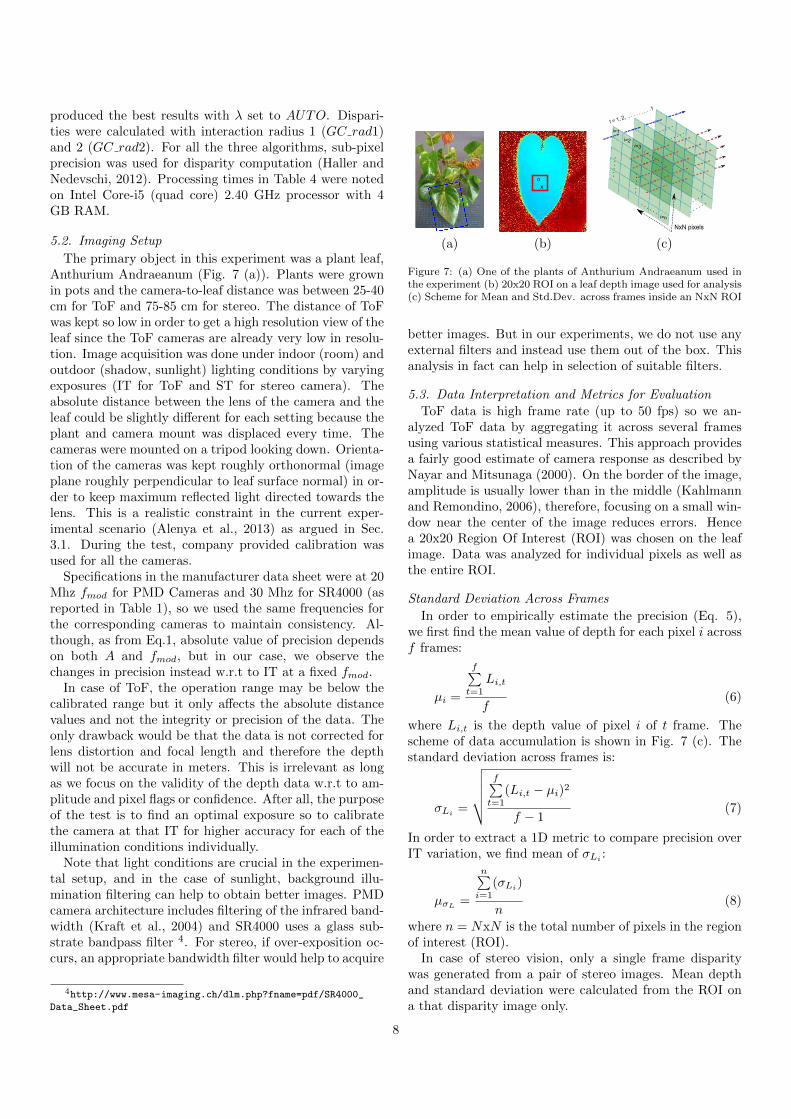
Figure 7: (a) One of the plants of Anthurium Andraeanum used inthe experiment (b) 20x20 ROI on a leaf depth image used for analysis(c) Scheme for Mean and Std.Dev. across frames inside an NxN ROI

better images. But in our experiments, we do not use anyexternal filters and instead use them out of the box. Thisanalysis in fact can help in selection of suitable filters.

5.3. Data Interpretation and Metrics for Evaluation

ToF data is high frame rate (up to 50 fps) so we an-alyzed ToF data by aggregating it across several framesusing various statistical measures. This approach providesa fairly good estimate of camera response as described byNayar and Mitsunaga (2000). On the border of the image,amplitude is usually lower than in the middle (Kahlmannand Remondino, 2006), therefore, focusing on a small win-dow near the center of the image reduces errors. Hencea 20x20 Region Of Interest (ROI) was chosen on the leafimage. Data was analyzed for individual pixels as well asthe entire ROI.

Standard Deviation Across Frames

In order to empirically estimate the precision (Eq. 5),we first find the mean value of depth for each pixel i acrossf frames:

µi =

f∑t=1

Li,t

f(6)

where Li,t is the depth value of pixel i of t frame. Thescheme of data accumulation is shown in Fig. 7 (c). Thestandard deviation across frames is:

σLi =

√√√√√ f∑t=1

(Li,t − µi)2

f − 1(7)

In order to extract a 1D metric to compare precision overIT variation, we find mean of σLi

:

µσL=

n∑i=1

(σLi)

n(8)

where n = NxN is the total number of pixels in the regionof interest (ROI).

In case of stereo vision, only a single frame disparitywas generated from a pair of stereo images. Mean depthand standard deviation were calculated from the ROI ona that disparity image only.

8

Figure 8: CamBoard response in amplitude, depth and precision between 25-40 cm aggregated in a 20x20 (ROI) under room, full shadow andsunlight conditions for one leaf in view and a white wall. Good and Bad pixels are among the last and first ones to be flagged inconsistent,respectively (Table 2). Both pixels are inside the ROI (c) Inconsistent → Maxima shows the curve when inconsistent pixels are set tomaximum depth manually (d) Poly. Fit is the trend line for the mean Std.Dev. curve (blue line) of ROI (a) A quick glance shows CamBoardperformance in descending order as (iv) white wall: best to (i) room leaf: better, (ii) shadow leaf: satisfactory and (iii) sunlight leaf: worst.

5.4. Camera Response Analysis: PMD

Maximum value of amplitude in PMD cameras is above2.5x104 units. Fig. 8, 9 row (a) show mean amplitude forCamBoard and CamCube, respectively. The graph showscharacteristics for a single pixel and a 20x20 ROI on theleaf for room, shadow and sunlight conditions. In thesegraphs, good pixels are those that reach amplitude sat-uration and before that, their amplitude deviates fromlinearity in all the three conditions. Bad pixels on theother hand, exhibit a very unpredictable behavior and donot necessarily reach saturation amplitude at all. Due tothese bad pixels, the mean amplitude deviates from linear-ity much earlier.

Assuming the same material properties for all the pixelson the sensor of the camera, it appears that non-linearityis not related to amplitude maxima only. It may occur

even before. Fig. 8, 9 row (b) show the correspondingdepth values of pixels which start getting out of synchro-nization as soon as the corresponding amplitudes deviatefrom linearity. The IT range where this behavior occursis shown between dotted green bars, we call it the greenzone.

According to May et al. (2006) and also by our observa-tion, this deviation depends on the distance between theobject and the camera. For closer objects, it occurs earlier(lesser IT) than for distant objects. Similarly, it occursearlier for more reflective objects at a given distance, forinstance, the white wall in column (iv).

It can also be seen that ambient illumination affects thebehavior of the amplitude curve. Deviation from linearityoccurs earlier under sunlight (strong background illumina-tion) than in shadow and room conditions. If the IT is

9

Figure 9: CamCube response in amplitude and depth between 25-40 cm in a 20x20 (ROI) under room, full shadow and sunlight conditionsfor one leaf in view and a white wall. Good and Bad pixels are among the last and first ones to be flagged saturated, respectively (Table 2).Both pixels are inside the ROI (c) Saturated → Maxima shows the curve when saturated pixels are set to maximum depth manually (a) Aquick glance shows CamCube performance in descending order as (iv) white wall: best to (i) room leaf: better, (ii) shadow leaf: satisfactoryand (iii) sunlight leaf: worst.

Table 2: PMD Flags

Flag Identifier Description

Invalid 01(hex) Depth unreliable due tovery high or low amplitude

Saturated 02(hex) Amplitude saturationreached (CamCube)

Inconsistent 04(hex) Raw data inconsistent(CamBoard)

Low Signal 08(hex) Not enough signal strengthSBI Active 10(hex) Suppression of background

light active (CamBoard)

increased further than the green zone, the deviation con-tinues and worsens to a point that the PMD on-boardsystem sets inconsistent flag for the CamBoard and satu-ration flag for CamCube, which in-turn also sets the in-valid flag in both (Table 2). Inconsistency, according toCamBoard documentation, means multiple depth valuespertaining to one pixel or incompatible amplitude whichcan also be caused by saturation. In rows (a) and (b),good and bad pixels are among the last and first ones tobe flagged inconsistent/saturated, respectively.

As discussed in Sec. 4, depth precision is directly relatedto the amplitude of the received signal therefore amplitudemust be high enough to enable correct depth measurement,still below the saturation level. Amplitude increases withIT. In order to find the highest possible IT suitable fora given setting, let us consider the precision or standarddeviation (Eq. 8) in Figure 8 row (d). This standarddeviation is the mean precision of the ROI (Eq. 8). Sinceboth PMD cameras show similar trends in precision w.r.tmean amplitude and depth, so only CamBoard precisioncurve is used for analysis.

From the figure, in case of room conditions, the precisionis quiet low at very low IT. It improves with increasing IT.The most important part is the first valley of the standarddeviation or its trend line i.e. when precision is the highestfor the first time. This indicates that there is a consensusamong the values of one pixel across all the frames and forthe whole ROI. Any second valley will not be importantbecause it will be due saturation which would still bringconsensus among frames. The rise of the trend line afterthe first valley indicates fall of precision which is indicatedbetween red dotted bars, we call it the red zone. Numberof bad pixels start increasing somewhere in the red zone.But the depth or amplitude values may not significantlychange at this stage. They are just different from frame

10

ITL1

50Lμ

Lsec

sIT

L600

Lμse

csIT

L800

LμLs

ecs

(i)LRoom (ii)LShadow (iii)LSunlight

(a)

(b)

(c)

0 0.1 0.2 0.3 0.4 0.5 0.6 0.7 0.8 0.9 1meters

Original

Invalid Inconsistent

LowLLevel SBILActive

(d)

Figure 10: CamBoard: (a,b,c ) Depth images of plant leaves un-der the three different ambient illumination conditions. Inconsistentpixels appear as dark spots. (d) Flags set at 900 IT µs under roomconditions

to frame, due to which precision drops.In order to see the corresponding change in the mean

depth curve, we set the depth of the inconsistent or satu-rated pixels to a very high value as soon as the flags areset. The result is displayed (Fig. 8, 9 (c)). The sharp risein the curve indicates the IT at which the pixels are turn-ing bad. This provides us the upper threshold of the ITfor each ambient condition. The ITs at which the numberof bad pixels become significant is shown in Table 3. Inour general observation, the point where the green zonestarts usually lies at IT values 20-30 % below these values.

In other words, the appearance of inconsistent or satu-rated flag is an early warning of non-linearity of amplitudeand hence increasing IT any further will only worsen thecredibility of data.

In all the three conditions, the point with highest pre-cision lies is in the green zone. Shadow and room illu-mination conditions can widely vary which will shift thegreen and the red zones slightly. Still the flags serve asan indication. Fig. 10 and Fig. 11 shows some images ofleaves in the three illumination condition. The three ITvalues are those at which bad pixels are noticeable in oneof the illumination conditions. Fig. 10 (d) and Fig. 11(d) show flags set at IT 900 µs under room conditions forCamBoard and CamCube, respectively.

Comparison of Leaf with White Wall

Fig. 8, 9 column (iv) show the response of white wallat approximately 35-40 cm from the PMD cameras, ag-gregated in a 20x20 ROI, under room conditions. Whitewall is chosen in order to benchmark the ToF imaging forleaves as white wall is highly if not perfectly reflecting pla-nar surface, is fairly lambertian and such surfaces are usedfor measuring the ToF imaging quality (Kahlmann and Re-

Figure 11: CamCube: (a,b,c) Depth images of plant leaves underthe three different ambient illumination conditions. Saturated pixelsappear as dark spots. (d) Flags set at IT 900 µs under room

Table 3: IT for Saturation Thresholds

Sensor Environment IT (µs)

CamCube Room 750-do- Shadow 600-do- Sunlight 500CamBoard Room 700-do- Shadow 400-do- Sunlight 100SR4000 Room 800-do- Shadow (5KLux) 500-do- Sunlight less than 300

mondino, 2006). We compare it to the best characteristicsof the leaf images which is under room conditions (column(i)). In PMD cameras, wall characteristics are better thanleaf as the amplitude (a) and (b) are more synchronizedover the entire range of IT than the leaf. As already dis-cussed in Sec. 3.1 leaves have high transmittance in NIR,this could possibly be the cause of a slight late saturationmeanwhile the wall has stronger reflectance, therefore, anearlier saturation point. Other than that, the overall per-formance of the leaf under room conditions is quiet com-parable to that of the white wall. This validates furtherthe use of ToF imaging for leaf analysis.

5.5. Camera Response Analysis: SwissRanger

SwissRanger cameras produce a confidence matrix in-stead of flags, which serves a similar purpose. High confi-dence for each pixel is desired in order to guarantee reliabledata. The confidence is related to the precision.

Fig. 12 row (d) show the precision curve. Due to thehigh density of the data in PMD cameras (small step size:

11

Figure 12: SR4000 response in amplitude, depth and precision at 25-40 cm in a 20x20 (ROI) under room, full shadow and sunlight conditionsfor one leaf in view and a white wall. Good and Bad pixels are among the last and first ones to show low confidence, respectively. Both pixelsare inside the ROI. (d,iii) Observe the distinct trend in precision under sunlight due to rapidly increasing number of saturated pixels.

Table 1), a polynomial fit is used to display trends of meanstandard deviation while for the SR4000, sparsity of thedata produces abrupt and vivid changes. These abruptchanges make SR4000 data interpretation a lot easier thanPMD, yet it is a drawback in terms of fine tuning of thecamera parameters.

As can be seen from Fig. 12 (d), the first valley of meanstandard deviation (precision) is quite obvious (dashedhorizontal red line). The steep rise and subsequent sharpfall in precision reduces the green zone to almost a singleIT in columns (i),(iii) and (iv) or a very narrow band as incolumn (ii) unlike a range of IT values in PMD cameras.

Matching curves in row (d) to row (a),(b) show that thefall in precision is a consequence of appearance of bad pix-els. As soon as pixels’ amplitude deviate from linearity,depth values start getting out of synchronization, increas-

ing the mean standard deviation of the ROI. The changein the pattern of the data is reflected in the correspondingconfidence values (row (c)). The confidence stays high,as long as the mean amplitude maintains linearity. Badpixels carry low confidence. Therefore, as soon as the am-plitude linearity is disturbed, the mean confidence drops.The limiting value of confidence, in this case, is 120 units.It may be the case in general. Data corresponding to theconfidence below this mark is unreliable under any illumi-nation condition.

Fig. 12 column (iii) shows the performance of SR4000under sunlight. Since the lowest possible IT in SR4000 is300 µs (see Table 1) which is still high for sunlight opera-tion, the appearance of bad pixels is quite early and (d,iii)shows a very different trend in precision which is due toincreasing number of pixels reaching saturation. Fig. 13

12

Figure 13: SR4000: (a,b,c,d) Depth images of plant leaves underthe three different ambient illumination conditions. Pixels with lowconfidence appear darker. (e) Confidence images with varying ITunder room conditions

shows SR4000 depth image under the three different ambi-ent illuminations at four different ITs. The IT values arechosen so that low confidence in data is noticeable underone of the illumination conditions. Fig. 13 column (iii)shows that there is no IT value under sunlight at which areliable depth image can be obtained with SR4000. Hence,this camera is not suitable for operation under sunlight; afact clearly mentioned in the manufacturer’s documenta-tion. Fig. 13 (e) shows confidence images of SR4000 atdifferent IT’s.

Comparison of Leaf with White Wall

Fig. 12 column (iv) show the response of white wallunder room conditions, at approximately 35 cm from theSR4000 camera, aggregated in a 20x20 ROI. Again, as dis-cussed in Sec. 5.5, unlike PMD cameras, the sparsity ofthe data does not provide enough information of the grad-ual degradation of the data except the point of saturationor low confidence which appears earlier than the leaf underroom conditions. But like PMD cameras, the overall per-formance of the leaf under room conditions and also undershadow is quiet comparable to that of the white wall. Theearly saturation is due to the wall being more reflectivethan the leaf.

5.6. Stereo Depth Analysis

Stereo data acquisition is only varied by one parame-ter, i.e. exposure or Shutter Time (ST). Selected stereoalgorithms have several parameters to tweak for best per-formance. Showing variation in disparity w.r.t each oneis beyond the scope of this paper. Therefore, we chose

Table 4: Stereo Processing Times

Algorithm Time (secs)

Point Grey Triclops < 1Correlation 3Graph Cut 250 for 7 iterations

the best parameters as mentioned in Sec. 5.1.2 and variedthe support region only for calculating matching cost dueto which varying disparities were produced. Depth valueswere calculated by Z = fb/d where Z is the depth in me-ters, f is the focal length of the camera in pixels, b is thebaseline (distance between the centers of the two camerasin meters) and d is the disparity measured in pixels.

Fig. 14 rows (a) and (b) show the mean depth andstandard deviation, respectively, in a 20x20 pixels ROIon the depth image of the leaf. Here, the standard devia-tion represents error in the estimation of depth from stereomatching.

The leaf was at 80 cm. The retrieval of depth informa-tion seems similar in all the global and local algorithms.For instance, in case of room (a,i), all the curves stayaround 80 cm throughout the ST range which means thatthe sensor did not saturate. Although, their accuracy var-ied. As Triclops is optimized for a particular hardware andreal-time applications, it can only produce good results fora short range of ST between 20 ms to 100 ms. Due to in-built validation steps, it produced high standard deviationfor higher values of ST which is due to holes appearing inthe disparity image (Fig. 12(b,i)). This is because thedata was being discarded as it did not satisfy the valida-tion conditions. Non-Optimized version of local correla-tion performed better for the entire ST range with moreaccurate results for increasing support regions. This isalso the case for GC based algorithm. But to complementthis analysis, we must either obtain ground truth, whichin case of plants is a difficult task (Nielsen et al., 2007)or else compare them by visual inspection. Fig. 18 showsdepth images under room of all the algorithms used, forfew selected STs and support regions sizes. The ST selec-tion is based on patterns in the standard deviation curvesfrom best to worst indicated in Fig. 14 row (b) with redmarkers on the ST axis.

These images reveal more about the quality of the stereomatching. Even though, correlation based algorithms re-trieved depth with less noise (low std. dev.), specially forbigger support regions, the shape characteristics are muchpoorer. This is because the support regions act as averag-ing filter and with bigger windows, noise tends to reduce inthe ROI, but at the same time, edges are blurred produc-ing poor shape definition. GC on the other hand, appearsto produce reasonably well shapes of leaves over a widerange of ST and with fairly accurate depth estimates.

In case of outdoor conditions, saturation does occur.

13

Figure 14: Stereo vision: Mean depth and Standard Deviation at 30-35 cm in a 20x20 (ROI) under room, full shadow and sunlight conditionsfor one leaf in view (Fig. 7 (a))

Looking at Fig. 14 (b,ii) and (b,iii), the ST values beyondwhich stereo matching is not able to retrieve any reliabledepth information ends near 20 ms for shadow and 4 msunder sunlight. If exposure is increased beyond this, thesharp rise in standard deviation implies a quick loss ofdata which is due to sensor saturation. Selection of shut-ter times is hence important in different illumination en-vironments. Fig. 19 and Fig. 20 show depth images forselected STs under shadow and sunlight.

Even below the saturation threshold, there is a slightvariation in the performance as saturation is approached.Since the best depth image results w.r.t to shape are ob-tained with GC based stereo matching algorithm, so basedon that, Fig. 18 (d), 19 (d) and 20 (d) show that the bestST values are 90 ms, 2.5 ms and 1 ms respectively. Thepenalty of operating beyond these values changes with theenvironment and is maximum in case of sunlight.

5.7. Imaging Under Mixed Illumination Conditions

In outdoor applications, it is highly likely to encountera situation in which the leaf is partly under sunlight andpartly under a shadow. The shadow in such a case isbrighter than a complete shadow due to possible diffrac-tion of sunlight which means that the saturation will occursooner.

Fig. 15 and Fig. 16 row (a) show depth images of leavesunder sunlight with some part under shadow of the cameratripod, for CamBoard and CamCube, respectively. Im-ages at two different exposures are taken, one suitable for

shadow and other for sunlight. Leaf surface can be ob-served at different depths for lower ITs and partly satu-rated for higher ITs in both cases. This difference is moreobvious in the corresponding intensity images (row (b)) es-pecially with CamCube because it has more NIR emittersthan CamBoard. Images at higher ITs cannot be used, forobvious reasons of saturation, but lower IT is not feasibleeither.

In order to increase the dynamic range of the ToF cam-eras, we exploit cameras flags and replace the depth valuesof all the pixels with Inconsistent/Saturated flags set athigher ITs with the corresponding values from lower ITs.The results are shown in Fig. 15 and Fig. 16 (a,iii) and(b,iii). The net effect of combining the exposures, both indepth and intensity is better than the original. This ap-proach will require calibration for only two IT values andas discussed in Sec. 5.4 and we operate in the correspond-ing green zones (high precision) of the two ITs. Otherwise,we are either lower than green zone or well into the redzone of the two different ambient illumination settings.

For SR4000, confidence matrix can be used in place offlags for increasing the dynamic range. But as it is evidentfrom Fig. 13 column (iii), SR4000 does not work undersunlight.

In case of stereo vision, although the best depth imagesw.r.t shape in Sec. 5.6 were obtained at ST 2.5 ms undershadow and 1 ms under sunlight, but the shadow in caseof mixed lighting (as discussed earlier) is brighter than acomplete shadow. Fig. 17 shows color and correspond-ing depth images obtained from GC rad2 at four different

14

Figure 15: CamBoard images including both shadow and sunlightexposures. (a,iii) and (b,iii) show High Dynamic Range (HDR) im-ages after combining two different exposures (c) Flags set at IT 300µs

exposures. Owing to this brighter shadow, a good compro-mised is reached at ST 1.45 ms. With higher STs, edges ofthe leaf are being erased due to high specular reflectionson the section under sunlight (column (iv)).

Even though the dynamic range of stereo vision camerasseems sufficient for the task at hand, still, higher dynamicrange can be obtained by preprocessing both the left andright images using standard methods such as combiningimages with varying exposures (Mann and Picard, 1995)before applying stereo matching. Of course, this will fur-ther add to the efficiency constraints of the stereo vision.

6. Discussion

Analysis done in Secs. 5.4, 5.5 and 5.6 addressed the re-sponse of ToF and stereo vision independently. For stereovision, Fig. 14 show that, except for subtle variations,retrieval of depth information is almost same for any al-gorithm, whether local or global, unless further validationsteps are involved such as in Triclops. Stereo vision canwork on a wide range of exposures while ToF has a verylimited exposure under outdoor conditions or may not evenwork at all, such as SR4000. Among the ToF cameras usedin this work, PMD CamCube has better cancellation ofsunlight (Table 3) followed by Camboard while the SNRof SR4000 renders it useless under sun. But in any case,ToF sensors are generally more sensitive to sunlight thanstereo vision.

Figure 16: CamCube images including both shadow and sunlight ex-posures. (a,iii) and (b,iii) show High Dynamic Range (HDR) imagesafter combining two different exposures. (c) Flags set at IT 550 µs

Figure 17: Depth images obtained through stereo correspondence forscene involving both shadow and sunlight exposures (GC Only)

Stereo vision, on the other hand, has its own draw backs.Visual inspection of the depth images from both the Timeof Flight (ToF) and the stereo vision show that bettershape estimation can only be achieved with global match-ing algorithms such as GC which still is not as good asToF depth images. Algorithms using local correlation mayprovide sufficient depth information for tasks such as leafangle estimation and leaf motion tracking (Biskup et al.,2007), but accurate shape retrieval which is crucial for nu-merous other applications (such as 3D model creation orplant specie recognition using leaf shapes) the local algo-rithms are not suitable. Global stereo matching such asGC, are usually very time consuming (Table 4). Over theyears, several other stereo matching algorithms have ap-peared and older ones have evolved both in terms of accu-

15

Table 5: Leaf surface characteristics of the validation flower plants(based on inspection)

Thickness Roughness

Low Pelargonium Anthurium

Medium Hydrangea HydrangeaCyclamenOrchidaceae

High OrchidaceaeCyclamenAnthurium

Pelargonium

racy and efficiency 5. Still, an accurate algorithm with anefficient implementation over a specialized hardware can-not make it comparable to ToF (30-50 fps).

Analysis of Validation Data

In order to further validate these findings, we testedfour more flower families, namely Cyclamen, Hydrangea,Orchidaceae and Pelargonium. Together, they representa wide range of leaf characteristics varying in thickness,shape, surface roughness and texture as shown in Table5. As for the ToF cameras, we have already shown thatthe performance characteristics are related to amplitudenon-linearity (Secs. 5.4 and 5.5), so we only evaluated theamplitude characteristics under room conditions at 30-40cm range for this validation set (Fig. 21). The ampli-tude curves clearly show that the given set of variations inleaf characteristics have a minimal effect on the responseof ToF sensors. The subtle variations are contributed bychanges is relative camera to leaf distance and leaf thick-ness. PMD CamCube appears to be least affected by suchvariations.

Fig. 22 shows color and depth images retrieved fromboth ToF and stereo vision sensors. Stereo data was ob-tained under room conditions at 80 ms and ToF imagesat IT 400 µs. The exposures are chosen to be the oneswith best performance under room conditions followingthe analysis from Secs. 5.4, 5.5 and 5.6. Again, the resultsvalidate the findings since the best shape retrieval can beobserved among ToF cameras with PMD CamCube andSR4000 providing the best results followed by PMD Cam-Board. Among the stereo matching algorithms, again GChas better shape retrieval but still not as good as ToF sen-sors. The local correlation algorithms do not perform wellin this regard as well.

7. Conclusion

We have performed a detailed analysis and comparisonof the response of ToF and stereo vision for close range leafimaging under room, shadow and sunlight conditions. Incase of ToF, the comparison with flat white wall indicatesthe suitability of using ToF imaging for agricultural appli-cations. Since ToF cameras are sensitive to ambient light,

5http://vision.middlebury.edu/stereo/eval/

Figure 18: Depth images acquired through stereo vision under roomconditions. ST values are chosen from the trends in the std.dev. (seeFig. 14 (b,i) red markers on horizontal axis)

we have proposed a method to detect suitable IT for thethree commonly faced conditions using the appearance ofinconsistent/saturation flags or confidence matrices. Thisscheme can be extended to any ambient illumination set-ting and object in general. Choosing a specific IT for agiven condition allows higher accuracy through optimalcalibration for that IT which adds to the value of imagingin close range tasks. Stereo vision, although, is relativelymore robust to outdoor illumination than ToF, suffers dueto the correspondence problems along with the efficiencybottlenecks which make ToF more preferable, even underoutdoor conditions.

The advantage of stereo vision is its high resolution out-put which is unmatched by any ToF camera so far (ToFmax. resolution 200x200). This is the low ToF resolu-tion which demands such close range observation of plantorgans (less than half meter), otherwise, SNR of ToF sig-nal deteriorates. Given the rapidly evolving technology,it seems more likely that ToF sensors will bridge the gapand come up with more robust background illuminationrejection and higher resolution than stereo vision researchproducing highly accurate and efficient algorithms.

Generally, all stereo cameras and some ToF cameras(e.g. SR4000) have an option for selecting the exposureautomatically. But such automatic selection can compro-mise precision. The analysis presented in this article wasestablished on one type of plant and validated on fourother plant families. So it can be safely concluded thatToF imaging is suited for leaf imaging in general. Whilethe camera settings may change slightly, this article pro-vides a method to find optimal camera parameters for anyplant (object in general), ambient illumination and dis-tance.

16

Figure 19: Depth images acquired through stereo vision undershadow conditions. ST values are chosen from the trends in thestd.dev. (Fig. 14 (b,ii) red markers on horizontal axis)

Acknowledgments

This work is supported by the Danish Council forStrategic Research under project ASETA (www.aseta.dk)grant no. 09-067027, the Spanish Ministry of Scienceand Innovation under projects PAU + DPI2011-27510,the EU project GARNICS (FP7-247947) and the Cata-lan Research Commission (SGR-00155). Wajahat Kazmiis funded by ASETA and Sergi Foix is supported by PhDfellowship from CSIC’s JAE program. Authors want tothank PMDTec and Ilona Schwengber for their supportand insightful information about CamBoard and Cam-Cube.

References

Alenya, G., Dellen, B., Foix, S., Torras, C., 2013. RobotizedPlant Probing: Leaf Segmentation Utilizing Time-of-Flight Data.Robotics Automation Magazine, IEEE 20 (3), 50–59.

Alenya, G., Dellen, B., Torras, C., 2011. 3D modelling of leavesfrom color and ToF data for robotized plant measuring. In: IEEEInternational Conference on Robotics and Automation. Shanghai,China, pp. 3408–3414.

Andersen, H. J., Reng, L., Kirk, K., Nov. 2005. Geometric plantproperties by relaxed stereo vision using simulated annealing.Computers and Electronics in Agriculture 49 (2), 219–232.

Astrand, B., Baerveldt, A., 2004. Plant recognition and localiza-tion using context information. In: Proc. of the IEEE ConferenceMechatronics and Robotics. Luoyang, pp. 13–15.

Biskup, B., Scharr, H., Schurr, U., Rascher, U., Oct. 2007. A stereoimaging system for measuring structural parameters of plantcanopies. Plant, cell & environment 30 (10), 1299–308.

Blas, M. R., 2010. Fault-Tolerant Vision for Vehicle Guidance inAgriculture Fault-Tolerant Vision for Vehicle Guidance in Agri-culture. Ph.D. thesis, Denmark Technical University, Lyngby.

Brakke, T. W., 1992. Goniometric measurements of light scattered.In: 12th Annual International Geoscience and Remote SensingSymposium (IGARSS). pp. 508–510.

Figure 20: Depth images acquired through stereo vision under sun-light conditions. ST values are chosen from the trends in the std.dev.(Fig. 14 (b,iii) red markers on horizontal axis)

Chapron, M., Ivanov, N., Boissard, P., Valery, P., 1993. Visualiza-tion of corn acquired from stereovision. In: Proceedings of IEEESystems Man and Cybernetics Conference. Vol. 5. pp. 334–338.

Chelle, M., Sep. 2006. Could plant leaves be treated as Lambertiansurfaces in dense crop canopies to estimate light absorption? Eco-logical Modelling 198 (1-2), 219–228.

Feret, J.-B., Francois, C., Asner, G. P., Gitelson, A. a., Martin,R. E., Bidel, L. P., Ustin, S. L., le Maire, G., Jacquemoud, S., Jun.2008. PROSPECT-4 and 5: Advances in the leaf optical proper-ties model separating photosynthetic pigments. Remote Sensingof Environment 112 (6), 3030–3043.

Fiorani, F., Rascher, U., Jahnke, S., Schurr, U., Apr. 2012. Imagingplants dynamics in heterogenic environments. Current opinion inbiotechnology 23 (2), 227–35.

Foix, S., Alenya, G., Torras, C., 2011. Lock-in time-of-flight (ToF)cameras: a survey. Sensors Journal, IEEE 11 (9), 1917–1926.

Frasson, R. P. D. M., Krajewski, W. F., 2010. Three-dimensional dig-ital model of a maize plant. Agricultural and Forest Meteorology150 (3), 478–488.

Garcia, R., Francisco, J., Sankaran, S., Maja, J., Feb. 2013. Com-parison of two aerial imaging platforms for identification ofHuanglongbing-infected citrus trees. Computers and Electronicsin Agriculture 91, 106–115.

Gates, D., Keegan, H., Schleter, J., Jan. 1965. Spectral properties ofplants. Applied optics 4 (1), 11.

Govaerts, Y., Jacquemoud, S., Nov. 1996. Three-dimensional radi-ation transfer modeling in a dicotyledon leaf. Optical Society ofAmerica 35 (33), 6585–6598.

Haller, I., Nedevschi, S., Feb. 2012. Design of Interpolation Functionsfor Subpixel-Accuracy Stereo-Vision Systems. IEEE Transactionson Image Processing 21 (2), 889–98.

Ivanov, N., Boissard, P., Chapron, M., Andrieu, B., 1995. Computerstereo plotting for 3-D reconstruction of a maize canopy. Agricul-tural and Forest Meteorology 75 (13), 85–102.

Jacquemoud, S., Baret, F., Nov. 1990. PROSPECT: A model of leafoptical properties spectra. Remote sensing of environment 34 (2),75–91.

Jimenez, A., Ceres, R., Pons, J., 2000. A survey of computer visionmethods for locating fruit on trees. Transactions of the ASAE-American Society of Agricultural Engineers 43 (6), 1911–1920.

Jin, J., Tang, L., 2009. Corn plant sensing using real-time stereovision. Journal of Field Robotics 26 (6-7), 591–608.

Kahlmann, T., Remondino, F., 2006. Calibration for increased accu-

17

Figure 21: TOF amplitude characteristics of the four flower familiescomprising the validation set

racy of the range imaging camera SwissRanger. In: ISPRS Com-mission V Symposium. No. 4. Dresden, Germany, pp. 136–141.

Kazmi, W., Bisgaard, M., Garcia-Ruiz, F., Hansen, K., la Cour-Harbo, A., 2010. Adaptive Surveying and Early Treatment ofCrops with a Team of Autonomous Vehicles. In: European Con-ference on Mobile Robots. Orebro, Sweden, pp. 253–258.

Kazmi, W., Foix, S., Alenya, G., Nov. 2012. Plant leaf imaging usingtime of flight camera under sunlight, shadow and room conditions.In: Proceedings of International Symposium on Robotic and Sen-sors Environments. IEEE, Magdeburg, Germany, pp. 192–197.

Kise, M., Zhang, Q., Oct. 2008. Development of a stereovision sensingsystem for 3D crop row structure mapping and tractor guidance.Biosystems Engineering 101 (2), 191–198.

Klose, R., Penlington, J., Ruckelshausen, A., 2009. Usability study of3d time-of-flight cameras for automatic plant phenotyping. Born-imer Agrartechnische Berichte 69, 93–105.

Kolmogorov, V., Zabih, R., 2002. Multi-camera Scene Reconstruc-tion via Graph Cuts. In: Proceedings of the 7th European Con-ference on Computer Vision-Part III. ECCV ’02. Springer-Verlag,London, UK, pp. 82–96.

Kraft, H., Frey, J., Moeller, T., Albrecht, M., Grothof, M., Schink,B., Hess, H., Buxbaum, B., 2004. Elimination Based on ImprovedPMD (Photonic Mixer Device)-Technologies. In: OPTO, AMAFachverband. Nurnberg.

Kraft, M., Regina, N., Freitas, S. a. D., Munack, A., 2010. Test of a3D Time of Flight Camera for Shape Measurements of Plants. In:CIGR Workshop on Image Analysis in Agriculture. No. August.Budapest.

Kyto, M., Nuutinen, M., Oittinen, P., Jan. 2011. Method for mea-suring stereo camera depth accuracy based on stereoscopic vision.SPIE/IS&T Electronic Imaging: Three-Dimensional Imaging, In-teraction and Measurement 7864, 1–9.

Lange, R., 2000. 3D time-of-flight distance measurement with cus-tom solid-state image sensors in CMOS/CCD-technology. Ph.d.dissertation, University of Siegen.

Lange, R., Seitz, P., 2001. Solid-state time-of-flight range camera.Quantum Electronics, IEEE Journal of 37 (3), 390–397.

Mann, S., Picard, R. W., 1995. On being ’undigital’ with digitalcameras : Extending Dynamic Range by Combining DifferentlyExposed Pictures. Science (323), 422–428.

May, S., Werner, B., Surmann, H., 2006. 3D time-of-flight camerasfor mobile robotics. In: IEEE International Conference on Intelli-gent Robots and Systems. Beijing, China, pp. 790– 795.

McCarthy, C., 2009. Automatic non-destructive dimensional mea-

Figure 22: ToF (IT 400 µs) and Stereo (ST 80 ms) depth images ofthe four flower families comprising the validation set

surement of cotton plants in real-time by machine vision. Ph.D.thesis, University of Southern Queensland.

Mizuno, S., Noda, K., Ezaki, N., Takizawa, H., Yamamoto, S., 2007.Detection of Wilt by Analyzing Color and Stereo Vision Dataof Plant. In: Gagalowicz, A., Philips, W. (Eds.), Computer Vi-sion/Computer Graphics Collaboration Techniques. Vol. 4418 ofLecture Notes in Computer Science. Springer Berlin Heidelberg,pp. 400–411.

Moller, T., Kraft, H., Frey, J., Albrecht, M., Lange, R., 2005. Ro-bust 3d measurement with pmd sensors. In: Hilmar, I., Timo,K. (Eds.), Robust 3D Measurement with PMD Sensors, Proceed-ings of the 1st Range Imaging Research Day at ETH Zurich. No.Section 5. Zurich, Switzerland.

Mufti, F., Mahony, R., Sep. 2011. Statistical analysis of signal mea-surement in time-of-flight cameras. ISPRS Journal of Photogram-metry and Remote Sensing 66 (5), 720–731.

Mutto, C. D., Guido, P. Z., Cortelazzo, M., Mar. 2012. Time-of-Flight Cameras and Microsoft Kinect. In: SpringerBriefs in Elec-trical and Computer Engineering. Springer, Ch. 2, p. 21.

Nakarmi, A. D., Tang, L., 2010. Inter-plant Spacing Sensing at EarlyGrowth Stages Using a Time-of-Flight of Light Based 3D VisionSensor. In: ASABE Paper No. 1009216. St. Josheph, Michigan,pp. 1–15.

Nayar, S., Mitsunaga, T., 2000. High dynamic range imaging: spa-tially varying pixel exposures. In: Proceedings of Conference onComputer Vision and Pattern Recognition. Vol. 1. IEEE, pp. 472–

18

479.Nielsen, M., Andersen, H., Granum, E., 2005. Comparative study

of disparity estimations with multi-camera configurations in rela-tion to descriptive parameters of complex biological objects. In:International Archives of Photogrammetry, Remote Sensing andSpatial Information Sciences. Beijing, China.

Nielsen, M., Andersen, H. J., Slaughter, D. C., Granum, E., Jan.2007. Ground truth evaluation of computer vision based 3D re-construction of synthesized and real plant images. Precision Agri-culture 8 (1-2), 49–62.

Nielsen, M., Andersen, H. J. r., Slaughter, D. C., Giles, D. K., 2004.Detecting leaf features for automatic weed control using trinocularstereo vision. Minneapolis, USA.

Nuske, S., Achar, S., Bates, T., Narasimhan, S., Singh, S., Sep.2011. Yield estimation in vineyards by visual grape detection.In: IEEE/RSJ International Conference on Intelligent Robots andSystems. pp. 2352–2358.

Piron, a., Heijden, F. V. D., Destain, M., Nov. 2011. Weed detectionin 3D images. Journal of Precision agriculture 12 (5), 607–622.

Point Grey, R., 2012. Stereo Accuracy and Error Modeling.Preuksakarn, C., Boudon, F., 2010. Reconstructing plant architec-

ture from 3D laser scanner data. In: 6th International Workshopon Functional-Structural Plant Models. pp. 1999–2001.

Rovira-Mas, F., Zhang, Q., Reid, J. F., 2005. Creation of Three-dimensional Crop Maps based on Aerial Stereoimages. BiosystemsEngineering 90 (3), 251–259.

Santos, T. T., Oliveira, A. A., Aug. 2012. Image-based 3D digitiz-ing for plant architecture analysis and phenotyping. In: Saude,A. V., Guimaraes, S. J. F. (Eds.), Workshop on Industry Applica-tions (WGARI) in SIBGRAPI 2012 (XXV Conference on Graph-ics, Patterns and Images). Ouro Preto, MG, Brazil.

Scharstein, D., Szeliski, R., Apr. 2002. A Taxonomy and Evaluationof Dense Two-Frame Stereo Correspondence Algorithms. Interna-tional Journal of Computer Vision 47 (1-3), 7–42.

Slaughter, D., Giles, D., 2008. Autonomous robotic weed control sys-tems: a review. Computers and Electronics in Agriculture 1 (issue:2002), 63–78.

Song, Y., Glasbey, C., van der Heijden, G., 2011. Combining stereoand Time-of-Flight images with application to automatic plantphenotyping. In: Proceedings of the 17th Scandinavian Confer-ence on Image Analysis (SCIA 2011). Vol. 1. Lecture Notes inComputer Science, Springer Verlag, Berlin, pp. 467–478.

Takizawa, H., Ezaki, N., Mizuno, S., Yamamoto, S., 2005. PlantRecognition by Integrating Color and Range Data ObtainedThrough Stereo Vision. Journal of Advanced Computational In-telligence and Intelligent Informatics 9 (6), 630–636.

Tang, L., Tian, L. F. L., 2008. Real-time crop row image recon-struction for automatic emerged corn plant spacing measurement.Transactions of The ASABE 51 (3), 1079–1087.

van der Heijden, G., Song, Y., Horgan, G., Polder, G., Dieleman,A., Bink, M., Palloix, A., van Eeuwijk, F., Glasbey, C., 2012.SPICY: towards automated phenotyping of large pepper plants inthe greenhouse. Functional Plant Biology 39 (11), 870–877.

Van der Zande, D., Stuckens, J., Verstraeten, W. W., Muys, B., Cop-pin, P., Jun. 2010. Assessment of Light Environment Variabilityin Broadleaved Forest Canopies Using Terrestrial Laser Scanning.Remote Sensing 2 (6), 1564–1574.

van Henten, E., Marx, G., Hofstee, J., Hemming, J., Sarlikioti, 2011.Measuring Leaf Motion of Tomato by Machine Vision. In: Inter-national Symposium on Advanced Technologies and ManagementTowards Sustainable Greenhouse Ecosystems: Greensys, ISHSActa Horticulturae 952.

Woolley, J. T., May 1971. Reflectance and transmittance of light byleaves. Plant physiology 47 (5), 656–62.

Yoon, S., Thai, C., 2009. Stereo Spectral Imaging System for PlantHealth Characterization. In: ASAE, Annual international meet-ing.

19