individuals among commuters: building personalised...

Pervasive and Mobile Computing ( ) –

Contents lists available at SciVerse ScienceDirect

Pervasive and Mobile Computing

journal homepage: www.elsevier.com/locate/pmc

Individuals among commuters: Building personalised transportinformation services from fare collection systemsNeal Lathia a,∗, Chris Smith b, Jon Froehlich c, Licia Capra b

a Computer Laboratory, University of Cambridge, UKb Department of Computer Science, University College London, UKc Department of Computer Science, University of Maryland, USA

a r t i c l e i n f o

Article history:Available online xxxx

Keywords:Public transportPersonalisationUrban data mining

a b s t r a c t

This work investigates how data from public transport fare collection systems can beused to analyse travellers’ behaviour, and transform travel information systems thaturban residents use to navigate their city into personalised and dynamic systems thatcater for each passenger’s unique needs. In particular, we show how fare collection datacan be used to identify behavioural differences between passengers: we thus advocatefor a personalised approach to delivering transport related information to travellers. Todemonstrate the potential for personalisation we compute trip time estimates that moreaccurately reflect the travel habits of each passenger. We propose a number of algorithmsfor personalised trip time estimations, and empirically demonstrate that these approachesoutperform both a non-personalised baseline computed from the data, aswell as publishedtravel times as currently offered by the transport authority. Furthermore, we show how toeasily scale the system by pre-clustering travellers. We close by outlining the wide varietyof applications and services that may be fuelled by fare collection data.

© 2012 Elsevier B.V. All rights reserved.

1. Introduction

The proliferation of pervasive technology throughout urban environments, such as smart traffic meters, location-basedbus systems, and cellular data, increasingly provides realtime information about city dwellers’ location and mobility. Thisnewfound availability of rich streams of urban data has led researchers to investigate its potential to aid urban planners,designers, and policy makers. Aggregate spatio-temporal analysis of urban data – often referred to as the ‘‘pulse of the city’’– can reveal how people use andmove between designed spaces and uncover otherwise hidden urban flows and structures.For example, geo-tagged collections of photographs have been used to identify tourist attractions [1], GPS traces from taxishave been used to inform future urban planning [2], and shared-bicycle station occupancy data has been used to aid themanagement of bicycle fleets [3]. In this work, we examine how a similar set of data can be used to provide personalisedtransit information services to individual city dwellers.We focus on one domainwhere data containing individuals’ mobilitypatterns has yet to be leveraged to serve peoples’ needs: public transport. Historically, public transport information systemshave been centred on the system itself (e.g., location of the transit service, scheduled and estimated arrival times of trains orbuses). In the following, we seek to explore how fare-collection data, which captures how individuals use public transport,can both uncover differences between individual travellers as well as be leveraged to provide more accurate informationrelating to their travels. The role of personalisation is particularly critical in this context: by providing a service that suits

∗ Corresponding author.E-mail addresses: [email protected] (N. Lathia), [email protected] (C. Smith), [email protected] (J. Froehlich), [email protected] (L. Capra).

1574-1192/$ – see front matter© 2012 Elsevier B.V. All rights reserved.doi:10.1016/j.pmcj.2012.10.007

http://dx.doi.org/10.1016/j.pmcj.2012.10.007

http://www.elsevier.com/locate/pmc

http://www.elsevier.com/locate/pmc

mailto:[email protected]




http://dx.doi.org/10.1016/j.pmcj.2012.10.007

2 N. Lathia et al. / Pervasive and Mobile Computing ( ) –

individual traveller needs and preferences, public transport satisfaction and usagewill increase,whichwill invariably reducecongestion and pollution in city streets.

To date, two challenges have prevented the deployment of personalised information services in transport domains. First,user preference data has been considered notoriously difficult to collect without resorting to manual intervention [4].Second, even when user preferences are available, leveraging them successfully remains an open challenge. Recentdevelopments, however, offer new possibilities that promise to overcome these obstacles. On one hand, the introductionand widespread adoption of automated fare collection (AFC) systems throughout the world’s urban public transportnetworks provide an opportunity to collect users’ preferences and commuting habits (e.g., travel times, transportmodalities)of millions of travellers in an implicit and highly scalable manner. On the other hand, personalisation has become amainstreamandhighly active area of research in the context of Internet services, ranging frome-commerce,music, and newsrecommendation [5,6] to mobile location-based services [7]. Thus, there exists a vast toolkit of algorithms that have beensuccessfully used on web-based preference data that can potentially be applied to urban transport networks. In this work,we address questions that relate to linking these two fields of research: what does AFC data tell us about individual travellerpreferences and what sort of personalised travel services can be built from this data with personalisation algorithms?

1.1. Objectives and key results

In the following sections, we analyse a large, multi-modal, anonymised fare collection dataset of travellers using theTransport for London (TfL) public transport system. We do so from three perspectives: (i) the bird’s-eye, system-level view,(ii) comparing individuals to each other, and (iii) comparing individuals’ transit times to the published travel times fromtwo selected stations. In doing so, a number of key results emerge: first, whilst an analysis of system-wide aggregate datawould suggest all users follow the same pattern, individuals’ usage of public transport is not uniform. Fare collection datacan be used to uncover a series of emergent usage patterns that show a variety of travel habits. These more subtle usagesemerge when clustering travellers based on their temporal patterns in the transit network.

Furthermore, we find that published travel times (which fail to take individual differences into account) substantiallydiverge from, and, in particular, underestimate, actual travel times even when accounting for transfers. Based on theseinsights, we propose and evaluate a set of algorithms that provide travellers with personalised travel time estimates, andperform an in-depth spatial, temporal, and user-analysis of where estimation errors emerge. We close by proposing anddiscussing a wide range of personalised services that can be built using this data. We also formalise a number of predictionand ranking problems that underlie these applications, and lay the foundations for future work by discussing the potentialof augmenting AFC data with alternative repositories of traveller preferences.

1.2. Extensions to prior work

An earlier version of this work appeared in [8]. This paper extends our prior work in four main ways: first, we offer amore comprehensive analysis of travellers’ behaviours to gain valuable insights into why individual’s travel times vary. Forexample,we study trip distributions, temporal views of repeat trips, trip familiarity, aswell as the travel patterns that emergewhen clustering users based on travel time.We also conduct a novel enquiry that compares actual travel times (asmeasuredby the fare collection data) with published inter-station travel times as they appear on posters affixed at stations, furtherhighlighting the differences between static estimates and individual variations in transit times. Second, we compare ourpredictive techniques with static time-table based estimates, as offered by current travel planners; this new comparisonwas made possible after having obtained, via a public Freedom of Information request, detailed information about inter-station transit times for the entire London rail network. Third, we evaluate our prediction techniques on a complete dataset,that covers all users that travelled through the London rail network during a one-month period, as opposed to working withsamples of 5% of users as done before; we thus avoid biases that may have resulted from the sampling technique used—something which was outside our control. Finally, we analyse prediction errors from new angles: whilst in [8] we analysederror in relation to simple grouping of users, time of travel, and familiarity with a given route, we now offer a detailedanalysis of the temporal, spatial, structural, and user-trip characteristics of the experiments that we performed.

2. Smart card data from Transport for London

In this section, we describe the context of our study: measuring the differences that emerge between travellers who usethe public transport infrastructure in London, England. We first give a brief overview of the geographical span and reachof the infrastructure (Section 2.1) and of the fare collection system in use (Section 2.2); we then describe the data that weobtained from the transport authority (Section 2.3).

2.1. Transport for London

The public transport system in London consists of several interconnected subsystems, incorporating multiple modes oftransport. These include the London Underground, the Overground rail system, the Docklands Light Railway system (an

N. Lathia et al. / Pervasive and Mobile Computing ( ) – 3

automated train network operating in the east of the city), an extensive bus network, waterborne transport and portionsof the UK National Rail network. The London Underground is made up of 11 lines totalling 402 km of track, connecting260 stations1 whose locations range from central London to as far as Chesham, Buckinghamshire, which is approximately40 km from central London. Despite the name, only 45% of this network is actually underground. The transport network isseparated into 9 fare zones, with Zone 1 encompassing central London and higher numbers representing regions furtheraway from the centre of London, up to Zone 9, which contains a handful of outlier stations, including Chesham. The zoningsystem forms part of the fee structure for all rail travel in London, as well as approximating geographical distance from thecentre of London.

2.2. The Oyster Fare Collection system

Automated Fare Collection (AFC) systems are in use in a number of cities throughout the world including Seoul, SouthKorea, Buenos Aires, Argentina, Rostov, Russia, and Chicago, USA. In 2003, TfL introduced its own: an AFC systemwhich usesRFID-based smart card tickets called Oyster cards. The aim of this system is to replace all paper-based tickets with a singleticket that can operate across modalities: by 2008, TfL had issued over 16 million cards [9]; by 2009, this system accountedfor approximately 80% of all public transport trips in the city [10]. Detailed information about each trip is captured when anOyster card is used to enter or exit the public transport network. Beyond eliminating paper-based tickets, this automatedsystem introduces an important benefit: sequences of individual travellers’ trips can now be linked, allowing the transportoperator to build a fine grained record of all people’s movements within their network.

2.3. Oyster data overview

OurOyster card dataset contains every single journey taken on the system’s rail services using smart cards throughout the31 days of March 2010 (which contains 23 weekdays and 8 weekend days). This amounts to roughly 89 million journeys, ofwhich 70million are tube journeys, with the restmade up of trips taken onNational Rail, Overground and other rail systems.Each record details the day, anonymised user id, the origin and destination stations, entry time and exit time (measured asaccurately as the minute of entry/exit), as well as departure and arrival zone. We note, however, that the dataset does notcontain information regarding the actual route taken by individuals within the system but only their entry and exit points.Given the size and complexity of the London Underground network, there are often several distinct routes than can be takenbetween any two stations. To that end,whenwe discuss a ‘‘trip’’ or ‘‘journey’’, wemean a row of this data, which correspondsto an entry and exit of the system—we do not link or reason about adjacent entry/exit pairs of each user (which may indeedrepresent a multi-hop journey). Note also that in this paper we use ‘‘trip’’ and ‘‘journey’’ interchangeably.

We took two steps to clean the data. First, we removed any entries containing erroneous or inconsistent fields: entrieswere removed if the start time was earlier than the end time, or if the origin and destination were the same. Second, wefound that certain stations were represented by more than one unique identifier: these were consolidated into a uniqueid number for each station. Approximately 2.5% of journeys were found to have end times earlier than the start time; afurther 1.5% had the same origin and destination station and 0.5% of entries were repeated trips with the same start timebut multiple end times. There were a number of entries that we did not remove because we could not determine whetherthese were genuine or erroneous. These include, for example, trips lasting less than twominutes or as long as twelve hours.In these cases, we opted to retain the data because we did not want to risk altering the representativeness of the dataset.After cleaning the data, we are left with 96.4% of the original data, amounting to 76.6 million trips by 5.1 million uniqueusers—an average of 2.47 million journeys each day. We present a detailed analysis of this dataset next.

3. Analysing individual differences with Oyster data

There are three main hypotheses underpinning this work: (i) there exist fundamental differences between individuals’usage of public transport systems; (ii) these differences can be discovered by analysing AFC datasets; (iii) and, finally, thatthese individual differences can be used to build personalised travel services. In this section, we aim to validate the firsttwo hypotheses, by first showing how marked individual differences exist in the Oyster card dataset, and secondly bydemonstrating that these differences domatterwhen, for example, it comes to calculating travel times.Wewill then validatethe third hypothesis in Section 4.

We first look at the data as a whole, which elicits the one-size-fits-all traveller’s stereotype that emerges from anaggregate, system-level, perspective (Section 3.1). We then reveal how this bird’s eye view of the data masks an underlyingvariety of traveller characteristics (Section 3.2). Indeed, by using agglomerative clustering on the data, we highlight howdifferent travel habits emerge, each describing a different traveller’s ‘‘persona’’ with their own travel pattern (Section 3.3).Finally, having demonstrated that individual differences in travel patterns do exist, we quantify their magnitude whencalculating travel time: first, by comparing individuals’ actual travel times with respect to those of the whole crowd

1 http://www.tfl.gov.uk/corporate/modesoftransport/londonunderground/1608.aspx.

http://www.tfl.gov.uk/corporate/modesoftransport/londonunderground/1608.aspx


(a) Week day. (b) Week end.

Fig. 1. Aggregate temporal views of (a) weekday and (b) weekend rail activity in London based on our AFC dataset. Scheduled services typically runbetween 5:00 and 1:30 AM. Note the dominant two-spike commuter pattern present on weekdays but absent on weekends. Furthermore, the scale of(a) and (b) is not the same: in general, there is much less activity during the weekends.

(computed by aggregating all records in the AFC dataset—Section 3.4); second, by comparing static travel time estimates,published in posters affixed in tube stations, with respect to actual travel times as recorded in the AFC dataset, for tripstaking place within the Victoria tube line (Section 3.5).

3.1. The pulse of London: an aggregate system-level view

We begin our analysis by examining the aggregate usage patterns of the system. Later, we will contrast these aggregateresults with clusters of individualised travel behaviour. To quantify the system usage over a given period of time (e.g., a day)we define ametric of activity. First, we divide the period into a vector of equal sized time bins. Next, for each trip that starts attime to and ends at time td we increment each bin bi where to ≤ bi < td. Finally, we normalise the vector entries by dividingby the maximum observed value; this gives us a value between 0 and 1 representing the activity level at any one time. Weshow the results for weekday and weekend patterns in Fig. 1. Note that the normalisation was calculated independently forthe weekday and weekend graph (i.e., the y-axes between the two are not interchangeable).

The pattern in Fig. 1(a) clearly reflects commuting behaviour. This behaviour disappears during weekends (Fig. 1(b)),when a gradual increase in activity throughout the day emerges, peaking at approximately 18:25 before trailing off into theevening. The lowest activity levels occur between 2:00 and 5:00 AMwhen rail services are closed. Formost of the open hoursduring the weekday, the minimum activity level is just over 0.2—thus even during off peak periods the transit network isfairly well utilised. This mid-day lull is not apparent in the weekend graph.

Given that our AFC data also provides trip entry/exit timestamps, we can also examine aggregate patterns in travel timesin the London Underground network. From each trip tuple with start (entry) time to and end (exit) time td, the trip durationis simply (td−to)minutes. The globalmean trip timemeasuredwith the data is 28.41min (SD = 15.83min). Fig. 2(a) showsthe distribution of trip times which roughly follows a normal distribution with a long tail. To further explore the level ofconsistency in trip timeswhen the system is viewed as awhole, we also calculated themean and standard deviation for tripsbetween each possible pair of stations. Fig. 2(b) shows the cumulative distribution of standard deviations. Approximately86% of trips have observations with a standard deviation of less than 10 min, and around 32% have a standard deviationof less than 5 min. This indicates that despite the complexity, size, and diversity of available routes on the rail network inLondon, trip times are surprisingly consistent.

A coarse view of the London rail network’s usage thus reveals the following traveller model: a person who uses thenetworkmainly to commute to and fromwork,with a journey duration that is consistent over time and that is roughly half anhour long.However, given the sheer size of the rail network and thediverse population of London, such a simplemodelwouldlikely (or obviously) overlook other types of usage behaviours that don’t fit the average case: indeed, it would seem counter-intuitive for a variety of travellers (e.g., students, night-workers, tourists, pensioners) to fit these patterns. Unfortunately,our data lacks any features that would allow us to categorise travellers into these well-known groups, thus seeminglylimiting the applicability of using fare collection data to inform traveller information systems. In the following section, wedemonstrate that the Oyster data can be used to gather implicit differences between users. We apply clustering techniquesto merge them automatically into groups with similar behaviours: we then show how, with no explicit knowledge of whoeach traveller is (i.e., based solely on usage data), travel information systems can be augmented to provide tailored resultsto each traveller.

3.2. Individuals among commuters

For the commuter stereotype to hold for all travellers, we would expect the following: (a) as the dominant travelpattern is a commute to and from work, the majority of travellers would have an average of 2 journeys (or more) per day;


(a) Travel time distribution. (b) Standard deviation CDF.

Fig. 2. (a) The distribution of trip times showing that most trips are relatively short with a global average trip time of 28.41 (SD = 15.83) min. (b) CDF oftrip time standard deviation, showing that 86% of trip times are within 10 min of the respective trip mean.

(a) Trip count histogram. (b) Trip count CDF.

Fig. 3. (a) The distribution of trip counts and (b) the cumulative distribution of trip counts across each user over the 31 days in our dataset. There is asubstantial difference between users in terms of frequency of usage of public transport.

Table 1Groups of users and average trips per group: a small proportion of users onlytravel on weekends, and nearly half of the users in the data set only appearduring week days. Note, however, how those who travel on both week-daysand week-ends achieve double the trips per user average.

Users TripsSum Percentage Sum Avg/user

Week-day only 2,405,521 46.60 21,516,124 8.94Week-end only 395,209 7.66 917,763 2.32Both 2,361,787 45.75 56,407,420 23.88

Total 5,162,517 100 78,841,307 15.27

(b) furthermore, as the home and work place are not expected to vary much within a one month observation period, thesame origin–destination trips should be repeated over and over again; (c) finally, for most travellers, the first origin and thelast destination of the day should be the same, as this forms a closed loop with their commute. We now illustrate this isactually not the case, and that there exist many public transport passengers that do not fit this model. We then show howAFC data uncovers individual travellers’ implicit profiles.

(a) Average number of trips. Themean total number of trips per user across the 31 days of data is 15.27, approximately onetrip per user every two days: a significant proportion of travellers do not fit the commuting model. The differences go muchfurther: Fig. 3(a) plots the distribution of user trip-count over the month, while Fig. 3(b) plots the same data as a cumulativedistribution instead: as shown, the number of trips taken by each user ranges from 1 to well over 60, with the majority ofusers (66%) undertaking less than 1 trip every 2 days on average, and 2% (which still amounts to more than 100,000 users)taking more than 60 trips. Most notably, no more than 8% of users fit the expectation of 2 trips per weekday (that is, 46 ormore trips overall).

We further examined these differences by grouping users into those who travel only during week days, only weekenddays, and both: the sizes of each group (in terms of users, trips, and trips per user) are shown in Table 1. Nearly half of thetravellers in our dataset use transit only during weekdays (46.6%) while 7.7% only use transit on weekends (the remaining


(a) Proportion of repeated journeys. (b) Proportion of users forming a loop.

Fig. 4. (a) The proportion of user-trip observations that have been seen before. (b) The proportion of users who form a loop with their daily travels. Boththese results demonstrate the effect of the presence and absence of the commuting majority on weekdays and weekends respectively.

Fig. 5. Visualising the variance in the user’s spatial exploration of the city, by plotting the number of trips taken vs. stations visited. The blue line isthe mean, surrounded by the standard deviation in red. Note how the distribution changes near 50 trips in the month, which demarcates the differencebetween low-volume users and those who are using the system, on average, more than once a day. (For interpretation of the references to colour in thisfigure legend, the reader is referred to the web version of this article.)

45.8% of travellers use transit on both weekdays and weekends). Unsurprisingly, travellers who travel on both weekdaysand weekends average more trips overall in our dataset than the other two groups of travellers (AVG = 23.88, in the farright column in Table 1).

(b) Repeated trips. To examine repeat trip behaviour, we plot the cumulative number of user-trip pairs which have beenobserved previously as a proportion of the total number of trips observed thus far in Fig. 4(a). As time progresses, theproportion of repeated trips increases in a parabolic fashion, falling back slightly each weekend, and reaching 51.8% by day31. In other words, about half of the trips observed throughout an entire month have been taken at least once before, withthe other half being unique origin–destination tuples for that traveller during our period of observation (note: a differentperson may have taken that trip). Interestingly, in a study of over 250 car drivers, [11] found that the percentage of repeattrips reached 52.3% after 25 days of observation.

(c) Closing loops. Fig. 4(b) shows the proportion of users who form a loop each day. We count a user as having formed aloop if the origin station of their first recorded trip in a given day is the same as the destination of their last recorded trip thatday. The proportion of users forming a loop appears to follow a regular pattern, with approximately 50% looping onMondaythrough Thursday, 44% on Friday, and 37% on weekends. Note, however, that one limitation in this analysis is that we donot account for the spatial proximity of adjacent stations. That is, a traveller may leave from one station in the morning andreturn to another adjacent station in the evening. In our analysis, this would not be counted as a loop. However, even withthis limitation, approximately half of the travellers do close a loop in their daily trips.

(d) Trips vs. stations explored. Finally, we analysed the extent that usage of the public transport system (as measured bynumber of trips throughout the month) relates to spatial variance – in terms of the number of stations that the user’s visitin the network (shown in Fig. 5). We find that, for low-usage users, the total number of stations visited remains relativelysmall – varying between 5 and 15 stations in the entire month. An interesting pivot point in the distribution appears afterapproximately 50 trips in the month. This inflection point indicates that those travellers who use the transit system moreoften also achieve a higher coverage of stations in the train network. More research is needed to uncover why the inflectionpoint occurs near 50 trips.


(a) 3.15%. (b) 0.09%. (c) 2.45%.

(d) 0.56%. (e) 1.17%.

Fig. 6. Clusters that portray varying kinds of 2-spike behaviour, including travellers who depart before the morning rush-hour and return before, during,and after the evening commute. The percentage under each cluster denotes the proportion of the total data that fell into the given cluster.

3.3. Clustering travellers to uncover emergent behaviours

In this subsection, we cluster travellers according to their average daily temporal usage of the train network. The goalhere is to uncover patterns of behaviour that were not identified in the aggregate analysis above. To be able to comparetravellers to one another, we represent each of them as a numerical vector which describes their travel habits. We then usean unsupervised clustering algorithm to discover and visualise emergent groups of similar people. Due to the scale of thedata, we clustered random sub-samples of 2000 users, and repeated this process to generate a 10-fold cross validation ofcluster results. In the following, we describe the steps taken in each run in detail.

We first define travellers according to the week day times that they begin their trips; we split the 21.5 h day that thesystem is open for (from 4:30 till 2:00) into 5 segments, dividing the day around commuter hours (earlymorning 4:30–6:59,morning rush hour 7:00–9:59, day time 10:00–15:59, evening rush hour 16:00–18:59, and late evening 19:00–2:00). Wethen construct, for each traveller, a frequency vector of binned start times. That is, for each start time in the user’s set oftrips, the corresponding bin in the user’s vector is incremented. We decided to use 5 segments because of the sparsity ofthe data in terms of trips per user (see Fig. 3(a)): finer grained partitions of the start times (e.g., 10-min bins) would resultin many segments being empty, and thus presenting problems when measuring the similarity between vectors. We furtherpruned all users who had fewer than 2 trips in the entire data from this analysis to combat this issue.

Once we have a representation of each users’ temporal travel habits as a numerical vector of values, we can measure thesimilarity between any two travellers. Given a pair of vectors, a and b, where user a has taken a total of A trips and user bhas taken B trips, the similarity is computed as the absolute normalised difference between the vectors.

da,b =15

5i=1

aiA −biB

. (1)

Under this metric, smaller values represent higher similarity. Finally, we implemented a form of agglomerative hierarchicalclustering [12] to group travellers. This algorithm begins by assigning each user to an individual cluster, and then iterativelymerges the two most similar clusters until a threshold similarity value is reached. In other words, we first construct asimilarity matrix between all travellers, which will be populated with da,b values for each possible pair of travellers. Wethen select the minimum value from the matrix, and merge the two vectors that share this similarity value to produce anew cluster. When merged, the two original clusters become the members of the new cluster, and the centroid is calculatedas the mean of the member vectors. This process was continued until a maximum similarity value of 0.15 was reached;we found this value through a series of experiments. A similar clustering approach was used in [3] to automatically clustershared temporal usage behaviours across communal bicycling stations in Barcelona, Spain.

This approach resulted in 15 individual clusters. By visually comparing the temporal behaviour in each cluster, fourcategories of behaviour emerged. The first set, shown in Fig. 6, represents a variety of different 2-spiked trends, including:


(a) 7.15%. (b) 1.73%. (c) 3.18%.

(d) 2.58%.

Fig. 7. Clusters that portray varying kinds of evening-only behaviour.

(a) the typical commuting pattern, which appears in the aggregate data, (b, c) userswho first travel before themorning rush-hour, but returnwith the crowd, although those in (c) proportionally travel less during the evening peak hour, (d) users whotravel before themorning rush hour, peaking near 6:30AM, and then again late in the evening, peaking at 8:00 PM, and lastly,those who again travel early and then again before the evening rush-hour, at about 4:00 PM. In other words, even the dailycommuting habit is subject to a range of variants.

The other groups do not portray morning and evening travel habits. Instead, the travel patterns that emerge arecondensed into particular times of the day. Fig. 7 depicts clusters of those travellers who tend to use transit only towardsthe end of the day, portraying evening-only behaviour. These range from: (a) a two-spiked pattern that only emerges inthe evening, peaking near 6 PM and again near 11 PM; (b) a near two-spiked pattern that emerges even later during theday (7 PM–12 AM); (c) a set of travellers who begin moving after the morning peak hours and do so mostly throughout theafternoon rush-hour, and a similar set in (d) who exclusively travel throughout the evening peak-hour times.

The existence of travellers who exclusively use the system throughout the later hours of the day is counter-balancedby the third group (Fig. 8), with emergent patterns that centre on the morning hours only. Two sub-groups emerge: (a, b)morning travel with reduced usage throughout the day, and (c, d) morning only travel. Members of the latter sub-groupalso differ in terms of when they peak: (c) has members that travel during the ‘‘normal’’ commuting times, while (d) hasmembers who move much earlier.

Finally, the last group, in Fig. 8, (e) and (f), exhibit the remaining behaviour: their travel is centred on the middle hoursof the day. The difference between (e) and (f) is in terms of the variability in time-span: indeed, those in (f) produce – usingtheir week day travels exclusively – a travel pattern that resembles the aggregate week-end travel activity.

3.4. Travel time: individuals vs. the crowd

We now turn from exploring clusters of temporal usage patterns (i.e., when a traveller uses the transit system) toanalyzing individual differences with regards to travel time (i.e., how long it takes a traveller to get from A to B). To doso, we calculate two values: the average trip time for a given origin–destination pair mo,d, and the mean travel time for aparticular individual u’s trips between the same stations uo,d. These two values can be used to compare each individual tothe ‘‘crowd’’ of travellers who have travelled from o to d, by computing the normalised residual trip time ru,o,d for user u asfollows:

ru,o,d =uo,d − mo,d

mo,d. (2)

The normalised residual represents the average excess journey time that an individual traveller experiences compared tothe tripmean of all travellers. If ru,o,d is positive, this suggests that user u tends to be slower than average, whereas a negative


(a) 6.78%. (b) 0.17%. (c) 2.00%.

(d) 0.20%. (e) 10.65%. (f) 31.14%.

Fig. 8. Clusters that portray varying kinds of morning and day-time only behaviour.

(a) Residual vs observed familiarity. (b) Observed familiarity cumulative distribution.

Fig. 9. (a) Residual trip time becomes negative as users become more familiar, (b) note that 74% of user-trip pairs have familiarity of 1.

residual indicates that the user is, on average, faster than the crowd. We then count the number of times that u has takenthe trip between o and d as fu,o,d (which we denote as u’s observed familiarity with the trip), and compare the resultingresidual-familiarity pairs. The underlying intuition here is that, as users take a trip more frequently, they may no longerneed to pause to look at signs or read maps and will generally be more adept at moving about the system: does the dataconfirm this intuition?

Fig. 9(a) shows the resulting relationship between trip familiarity and average residuals. User average residuals do, infact, tend to become negative as the measured familiarity increases. This result has one limitation: the one-month viewthat we have of the data does not necessarily mean that, when we measure a traveller’s familiarity with an (o, d) pair tobe 1, the traveller has only ever taken the trip once. The user may very well have taken the trip previously, outside of thebreadth of data available to us. That said, we remain sure that the user only takes this trip once during the month-long viewthat we possess; therefore, while the user may not necessarily be taking this trip for the first time, it is likely that this isnot a high-frequency trip for that user. We examined the distribution of familiarity values closer in Fig. 9(b), which plotsthe cumulative distribution of familiarity among user trip means. Notice that for more than 74% of user-trip means, thefamiliarity value is 1, which suggests that the group of users who make a given trip once within the month contribute themost towards establishing the mean time.


(a) Warren Street station. (b) Euston station.

Fig. 10. An example poster with travel times from (a) Warren Street’s and (b) Euston’s Victoria line platform.

3.5. Travel time: individuals vs. static timetables

The last step of our analysis focuses on a comparison between individuals’ actual travel times, as recorded by our AFCdataset, and transit-time information provided by the London Underground. More precisely there are posters affixed inmost platforms stating how long it should take to travel to any destination that is reachable from the given platform alongthe same tube line (i.e., requiring no interchanges). In particular, we selected two stations on the Victoria Line (Euston andWarren Street, with posters shown in Fig. 10). The advertised travel times range from 2 min to reach an adjacent station, to19 min to reach the end of the line. We note that, although the stations are adjacent to one another, the listed travel timesare not symmetrical: Euston to Walthamstow Central is advertised as an 18 min trip. Warren Street, which is 2 min (and 1stop) from Euston, shows a 19 min journey to Walthamstow Central (rather than an 18 + 2 = 20 min trip). We have nofurther details about these travel times: we do not know how they are computed or what they assume; a matter that weleave for future investigation. However, by being a source of information for travellers, the estimates they display shouldoffer a relatively accurate picture of the amount of time necessary to travel between each pair of stations. How close areadvertised transit estimates to the travel time measured by AFC datasets?

We measured how actual travel originating at these stations and completing at any other station on the same line,compares to the poster’s expected trip duration. The results are shown in Fig. 11: blue bars represent the advertised numberof minutes from that station captured on the posters, while grey bars represent the mean travel time for all observed tripsbetween the given (o, d) pair, with red lines illustrating the variance. For example, the topmost bar in Fig. 11(a) is the meantravel time between Warren Street and Walthamstow Central.

The results show that actual mean trip times are much higher than listed times; indeed, the advertised times fall wellunder one standard deviation from each actual mean. The standard deviations are particularly large when travelling toadjacent stations. This may be explained by the fact that the transport authority is only advertising the train travel timebetween stations. Recent work [13] states that, on average, only 46%–62% of the time that users spend in the tube is actuallyspent riding the trains, while the rest is spent interchanging, walking, or waiting. These times, which are unaccounted forin static timetables, are still within the scope of the travellers’ perceived travel time; furthermore, while ‘time on train’ islikely to be the same for all travellers, it is precisely these times spent elsewhere within the system that we expect to varyacross individuals, and to account for the differences between individuals’ travel times and the crowd already highlightedin Fig. 9(a).

3.6. AFC data analysis conclusions

Based on the analysis conducted above, we draw the following three main conclusions:

• More than one traveller type exists. An aggregate analysis of the whole AFC data produces a single view of the underlyingtravellers, which is dominated by the commuting habits of a large subset of users. By using hierarchical clustering, we


(a) FromWarren Street.

(b) From Euston station.

Fig. 11. Travel time from Euston and Warren Street: the blue bars represent the advertised travel time from posters at each station, while the grey barsare the mean travel time as measured with the Oyster data. Note that, even when plotting the variance as well (in red), most values are underestimatedby the poster’s times. (For interpretation of the references to colour in this figure legend, the reader is referred to the web version of this article.)

showed that a number of different travel patterns emerge, thus discounting the value of modelling travellers using asingle perspective.

• The crowd’s travel time significantly differs from that of the individual travellers. The aggregate system view fails not only todescribe the travel patterns of the majority of travellers, but also to capture the time it takes for individual travellers tocomplete their journeys. For example, we showed that as a user becomes more familiar with a trip, the time it takes tocomplete the trip decreases.We thus cannot use information about the crowd as awhole to accurately describe individualtravel times.

• Published travel times fail to capture substantial differences in travellers’ transit times.Wecannot compute individual’s traveltimes using aggregate AFC data, and nor can we do so by using published travel time estimates. Indeed, as the last partof our analysis demonstrated, the advertised inter-link times consistently (and grossly) underestimate the time that ittakes people to travel between an origin and destination.


The analysis above thus demonstrates that there exist substantial differences among individual travellers, and that suchdifferences are indeed measurable via the implicit behaviours captured by the Oyster AFC system. So what can this data beused for?We posit that AFC data can be used to build more personalised travel information services, that is, services that aregeared towards the individual needs and characteristics of each single traveller. As a quantifiable example of such systems,in the next sectionwe delve into the construction of a personalised trip time estimator. In particular, we propose a variety ofprediction algorithms that leverage AFC data to implicitly capture individual travellers’ characteristics, and thus accuratelyestimate personalised travel times.

4. Trip time prediction algorithms

In this section, we explore a number of methods that take advantage of a user’s AFC-based travel history in order toprovide personalised trip time estimations. Recall that each data point gives us the origin, destination, and start and endtimes of each trip. As such, the following prediction models do not include information regarding the route taken betweenstations or service disruptions, both of which are likely to affect travel times. Instead, the models described here explore thepatterns and relationships highlighted in Sections 3.3 and 3.4, but with a specific focus on the differences between users.

4.1. Baselines

We first describe two baseline predictors against which the quality of our models will be assessed. The first baselineis based on the static travel time between adjacent stations. This data was obtained using a Freedom of Information(FOI) request2 to Transport for London; it details the distance and travel time between adjacent stations in the LondonUnderground network. This data does not include scheduled train departure or arrival information, only link traversal times.For example, for a train line with stations s1 ↔ s2 ↔ s3, the FOI data includes tuples with the travel time (t) between eachinterconnected station: ⟨s1, s2, t1⟩, ⟨s2, s3, t2⟩. Note that the FOI request returned travel time data from September, 2008whereas our AFC dataset is fromMarch, 2010 (18months later). We assume that travel times have not changed significantlyin those 18 months. The time between non-adjacent stations was computed using Dijkstra’s algorithm on a graph whereeach station is represented as a node, and the connections between each station are edges weighted by the link traversaltime: this method therefore produces the shortest path between any pair of stations based on hop-count (instead of, forexample, minimising number of transfers between lines); in the following sections, we refer to this as the static predictionmethod. Where an interchange occurs, we had a choice about howmanyminutes should be added to the total trip time: weexperimentally determined this ‘‘transfer time penalty’’ to be 8 min (see Section 5.2.1).

Although the Oyster data contains 584 stations, the FOI request provided us with link traversal times that included only355 (those covered by the London Underground), including all but one tube station. We therefore pruned trips betweenstations not present in the FOI request when testing all of the prediction algorithms.

The second baseline we use is derived from the Oyster data itself: the historical trip time average. This approach willnot take into account any differences between travellers, and simply returns the mean travel time for all trips between anygiven two stations. More formally, for the set To,d, which contains N observations of a journey between stations o and d, thebaseline estimated travel time is simply the arithmetic mean of all xt ∈ To,d, where xt denotes the travel time:

mo,d =1N

To,d

xt . (3)

4.2. Personalised approaches

Given the two baselines above, we now set out to design and evaluate algorithms that account for the differencesbetween users when making their predictions: such techniques could be used to provide personalised trip time estimatesto travellers using the system. In particular, the techniques that are presented in the following sections build off the latterbaseline by using different dynamic techniques to subsample the training data that is used to predict each user-trip pair.In particular, three types of information are leveraged: (a) the similarity between the current user and those who havehistorically travelled at the same time, (b) the similarity between the current user and those who have historically made thetrip with similar frequencies, and (c) the extent that each traveller will repeat past behaviours.

There are two main challenges that we faced when designing personalised trip estimate algorithms using the Oysterdata. First, the data is incredibly sparse and subject to each users’ habits; we thus do not hold a complete view of howtravel time over all (o, d) pairs varies with, for example, time of day. We address this below by weighting personalisedpredictions with the mean travel time, based on how much data is available. Second, the data is subject to noisy entries,such as when users encounter delays or other events whose occurrence significantly changes their normal travel time. Wedetermined empirically that computing a geometric mean provided a more robust estimate when taking small samples of

2 www.whatdotheyknow.com/request/distance_between_adjacent_underg.

http://www.whatdotheyknow.com/request/distance_between_adjacent_underg


data for personalised predictions. Given a set So,d of M observations of a given travel time between o and d, the geometricmean is computed as the log-sum of each member t:

go,d = exp

1M

So,d

ln t

. (4)

In the following sections, all references to amean of data sampled using a given method refer to the usage of the geometricmean.

4.2.1. Trip context modelThe first model aims to derive a trip time estimate by incorporating historical contextual information of each trip

that users are taking. Ideally, such an approach would take into account each trips’ details, including purpose of travel(e.g., business or leisure), service status, whether the user is travellingwith luggage or children, etc.. However, we are limitedby the information contained in the dataset and are therefore constrained to that which implicitly represents travellers’context: the historical average travel time for a journey at a particular time of day. We assume that, for a given start times and a time interval w, all users who start a journey from station o to station d within a window of size 2w centred on s,experience a similar context. Thus we can define wo,d as the geometric mean of the set of trip times Wo,d ⊂ To,d in whicheach observation xo,d,t meets the condition:

(t − w) ≤ s ≤ (t + w). (5)

The observationwindowdefined above operates at the day level: factorswhich vary above this level, such as holiday periodsand busy local events are not taken into consideration. Due to the sparsity of the data, the possibility exists that, for certain(o, d) pairs, the wo,d value will be undefined. When computing the personalised prediction p̂u,o,d,s, we compensate this byreturning a weighted combination of the window mean and the trip mean. We weight each component by the value M

N ,where we have a total of N observations of trip o, d, and M observations within the predefined window; this weightingallows us to compensate for data sparsity by using the aggregate data where necessary.

p̂u,o,d,s =

1 −

MN

× mo,d

+

MN

× wo,d

. (6)

4.2.2. Estimating with trip familiarityWhile the model above only considered the implicit similarity shared by travellers based on when they travel, the next

model incorporates notions of how familiar those users arewith a given trip. In Section 3.4we introduced the notion of user’sfamiliaritywith a trip, which is simply the number of timesM we have observed the user-origin–destination tuple. We alsofound an aggregate inverse relationship between the familiarity and the deviation of the user mean from the trip mean:those who had taken the trip with high frequency tended to travel faster. We capture this relationship when computingpredictions with the following definition: for a user u who has taken a trip between o and d a total of M times in the past,we define a neighbourhood of user means FM,o,d ⊂ To,d from users whose familiarity fo,d with the trip is such that:

M2

≤ fo,d ≤ 2M. (7)

In otherwords, we compute a personalised prediction for a user by identifying, using a slidingwindow, those userswho havehistorically taken the trip a similar number of times. To compensate for the sparsity of observations, we return a 1

M -weightedcombination of the trip mean and the familiarity mean:

p̂u,o,d,f =

1M

× mo,d

+

1 −

1M

× f o,d

. (8)

4.2.3. User self-similarity predictionsThe final model relies on the assumption that users may tend to exhibit consistent habits when navigating the system,

including their choice of route and walking pace; in effect, it assumes that travellers’ time spent in the system is likely to bemore similar to their own historical travel times than, unlike above, those of others. More formally, let Uo,d ⊂ To,d denotethe set of user u’s trip times between stations o and d. We compute the geometric mean uo,d, for each trip uo,d ∈ Uo,d.

As above, due to the sparsity of the data, the user mean will be undefined for many (o, d) pairs (where the user has notpreviously made that trip within the scope of the training data), or it may be the result of very few observations. To accountfor this, the personalised prediction p̂u,o,d returned by the user self-similarity model, is a 1

M -weighted combination of thetrip mean and user mean:

p̂u,o,d =

1M

× mo,d

+

1 −

1M

× uo,d

. (9)


Table 2Mean Absolute Error prediction results. The results are presented for allpredictions (aggregate) as well as decomposed into groups of users, who travelon week days only, weekend days only, and both week day and weekend days.Estimating users’ travel time based on how they travelled previously is, onaggregate, the most accurate method. However, travel time (context) becomesmore accurate for those users who only travel on weekends.

Method Mean Absolute Error (minutes)Aggregate Week day Week end Both

Static 9.82 9.91 10.71 9.72Trip mean 3.30 3.32 3.69 3.28

Context 3.28 3.29 3.68 3.26Familiarity 3.17 3.18 3.69 3.16Self-similarity 3.13 3.11 3.81 3.14

5. Evaluation

In the above, we have defined three perspectives of historical travel time data (context, familiarity, self-similarity) thatcan be used to forecast how long it will take a traveller to transit between an origin and destination. In this section, we usethe Oyster data in order to evaluate the accuracy of these forecasts, compared to the trip times that are estimated by bothbaselines. Recall that our dataset spans an entire month and includes 76.6 million trips. We test our prediction models byrepeatedly splitting the Oyster data into two partitions: a 1-day test set taken from the final week of the data, with all daysprior to it as a training. We repeated this procedure for each of the 7 final days in the dataset in order to provide 7-fold crossvalidated results, each of which has an approximate split of 95% training data to 5% test data. We next describe the accuracymetrics we used and the results we obtained (Section 5.1), and a detailed analysis of the user, spatial, and temporal aspectsof the accuracy achieved (Section 5.2).

5.1. Metrics and aggregate results

We use two metrics to evaluate the prediction accuracy: the Mean Absolute Error, MAE, and Mean Absolute PercentageError, or MAPE [14]. The MAE is measured in the same units as the trip times (minutes) and is simply the average absolutedifference between the actual trip time and the corresponding predicted trip time. Let N be the size of the test set, then foreach of N predictions, p̂u,o,d of user u’s time to travel from o to d, and the actual trip time xu,o,d:

MAE =1N

|xu,o,d − p̂u,o,d|. (10)

Table 2 compares the results from each model to the baseline predictions. As expected, the static link traversal-based dataprovides the least accurate forecast of travel time; on average, its estimates have an average error of 9–11 min. The tripmean that is computed using the Oyster data, instead, already provides a much stronger estimate. Yet it is outperformed byeach of the personalisedmodels, with the best performance provided by the self-similaritymodel, which tends to achieve anerror just above 3 min—roughly comparable to the average waiting time between trains. Self-similarity, however, is not asaccurate as using the time of travel (or context) for those users who travel exclusively on weekends. A potential explanationfor the loss in performance is the fact that this is the group of users who have, on average, the smallest number of trips perperson; prediction accuracy using the self-similarity method will thus begin to revert back to the trip mean. Fig. 12 displaysthese results visually for direct comparison.

An alternative view of the error can be obtained by normalising the absolute difference between the predicted and actualtravel time using travellers’ actual transit time, allowing us to compare errors for trips of varying length. TheMean AbsolutePercentage Error (MAPE) does just this: it is the error measured as a percentage of the actual trip time and produces valuesin the range 0%–100%.

MAPE =100N

|xu,o,d − p̂u,o,d|

xu,o,d

. (11)

Table 3 shows the MAPE results, grouped as before: they highlight that up to 40% of travel time may be unaccounted forwhen using static estimates. This result echoes previous research by Jang [13] described above, which claimed that 46%–62%of travel time remains unaccounted for when exclusively using train time. Moreover, while the self-similarity method onceagain appears to be themost accurate on aggregate and the context method overtakes all others for weekend only users, theMAPE metric gives a higher priority to the familiarity technique for those travellers who take trips on both kinds of days.

5.2. Error analysis

In the previous section, we presented empirical results that demonstrate the improved accuracy in travel time estimationwhen using fare collection data. In this section, we delve further into the accuracy of the above methods, in order to fully


Fig. 12. MAE results, when users are grouped by when they travel (weekdays only, weekends only, both). The results show varying behaviours from theprediction methods: for example, users who travel during both weekdays and weekends are the most accurate group when using the trip mean, but theleast accurate group when using self-similarity values.

Table 3MeanAbsolute Percentage Error prediction results. These results portraya similar trend to those reflected in the MAE results; however, thefamiliarity method overtakes the self-similarity method for thosetravellers who travel during both weekdays and weekends.

Method Mean Absolute Percentage ErrorAggregate Week day Week end Both

Static 37.67 37.26 40.62 38.03Trip mean 13.42 13.20 14.39 13.62

Context 13.35 13.13 14.37 13.57Familiarity 12.61 12.37 14.41 12.83Self-similarity 12.52 12.13 15.19 12.88

14

13

12

11

10

9

8

7

6

5

4

Mea

n A

bsol

ute

Err

or

Interchange Time (Minutes)

Static Esimation with Varying Intemchange Time

0 2 4 6 8 10 12 16 1814

Fig. 13. The relationship between static transfer times and trip estimation mean absolute error. Lower values imply more accurate trip time estimates: inthis work, we compare our proposals to the most accurate results found here (8 min).

understand the effect of static transfer times as well as how and where personalised approaches succeed. We investigatethe extent that error is distributed over a number of attributes, including the time and day of the trip, the trips’ length,the users’ familiarity, and the spatial and transport network/structural properties of the journey. For the sake of clarity, wecompare the static link traversal-based journey length estimates to the personalised self-similarity based predictions, whichwas found to be the most accurate method.


(a) Weekday. (b) Weekend.

Fig. 14. The difference in accuracy over an average weekday and weekend: during the week day, the static data suffers from a rush-hour effect, while thedata based approach remains flat.

5.2.1. Static transfer timeWe first examine the impact of changing the inter-line transfer time penalty in the link traversal-based prediction

method. We ran a series of experiments to determine which transfer time produces the most accurate results on the Oysterdata we have. Fig. 13 plots the results: a transfer time of 8 min was the most accurate; lower values were likely to be under-estimating travel time, while higher values begin to unnecessarily apply too much time to transfers. Note, however, thatthis value remains constant across all users.

5.2.2. Error by time of dayWe first investigate the variation in error values as the temporal attributes of the data vary. Fig. 14 shows the difference

in error between the static and self-similarity predictions according to the time of day for weekday (Fig. 14(a)) andweekend(Fig. 14(b)) trips. The upper bound of the standard deviation of data-based predictions is (with the exception of one point)consistently below the mean of the prediction errors when using the static method. Moreover, static predictions seem tosuffer fromapeak-hour effect: themean ofweekday predictions increases during the rush hour times. On the other hand, thedata-based predictions, which will capture how individuals tend to transit throughout the system, remains flat throughoutthe day and does not show this effect: in essence, personalised approaches overcome the challenge and need to dynamicallymodify trip estimation algorithms when the transport system is congested.

5.2.3. Accounting total travel timeAlthough personalised travel time estimation does not vary with the time of day, it may vary with the length of the trip

that the user is taking: are the techniques able to better predict short or long trips? To answer this question, Fig. 15 illustratesthe relationship between prediction error and the actual journey time. These results show how prediction errors tend to beproportionally higher for shorter trips. In fact, as trip lengths become longer, although the error increases, the proportionalerror becomes smaller; this points towards the fact that the less time travellers spend on trains, the more their individualdifferences will both emerge and determine their total travel time. Furthermore, when taking the standard deviations intoaccount, the static and self-similarity distributions only begin to overlap after approximately 50-min long trips; recall thatthe analysis above indicated that majority of trips taken in the system have a travel time far below this threshold.

5.2.4. Personalised approaches are not spatialIn the trip time estimation methods presented above, we did not take any spatial features of the city into account: we

now turn to this view of the data in order to visualise any potential spatial effects that emerge from the user-trip data.We hypothesise that the diversity of users entering stations in central London will be higher than, for example, stationsin residential areas, and that most of the time estimate errors will thus emanate from the city centre. In other words, weexamine the extent that trip time estimate errors vary according to the origin station of users’ trips. To do so, we computethe average error of all trips beginning at each station, computing oneMAE value for each origin in our dataset. We then plotthe distribution of the results in Fig. 16(a) and examine the spatial distribution of error in Fig. 16(b). The former shows thatthere is indeed a non-uniform distribution of error (i.e., the origin station relates to the amount of error in the trip forecast).However, we did not find any direct relationship between error and the location of origin stations: stations of varying errorare dispersed throughout the entiremap of London, bothwithin central London and outside of the confines of the city centre(16(b)). An analysis of the trip destinations’ reveals similar results. A likely explanation for this result stems from the fact thatour prediction algorithms do not use any spatial or structural information when computing trip estimates: the distributionof error may thus be more related to the origin–destination pair, as well as the amount of data available for the given pairand user who is taking the trip.


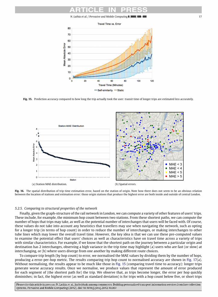
Fig. 15. Prediction accuracy compared to how long the trip actually took the user: transit time of longer trips are estimated less accurately.

(a) Station MAE distribution. (b) Spatial errors.

Fig. 16. The spatial distribution of trip time estimation error, based on the station of origin. Note how there does not seem to be an obvious relationbetween the location of stations and estimation error: those origin stations that produce the highest error are both inside and outside of central London.

5.2.5. Comparing to structural properties of the networkFinally, given the graph-structure of the rail network in London, we can compute a variety of other features of users’ trips.

These include, for example, the minimum hop count between two stations. From these shortest paths, we can compute thenumber of hops that trips may take, as well as the potential number of interchanges that users will be faced with. Of course,these values do not take into account any heuristics that travellers may use when navigating the network, such as optingfor a longer trip (in terms of hop count) in order to reduce the number of interchanges, or making interchanges to othertube lines which may lower the overall travel time. However, the key idea is that we can use these pre-computed valuesto examine the potential effect that users’ choices as well as characteristics have on travel time across a variety of tripswith similar characteristics. For example, if we know that the shortest path on the journey between a particular origin anddestination has 2 interchanges, observing a high variance in the trip time may highlight (a) users who are fast (or slow) atinterchanging, or (b) where users diverge from one another by making different route choices.

To compare trip length (by hop count) to error, we normalised the MAE values by dividing them by the number of hops,producing a error-per-hop metric. The results comparing trip hop count to normalised accuracy are shown in Fig. 17(a).Without normalising, the results appear to be much like those in Fig. 15 (comparing travel time to accuracy): longer tripsgenerate worse accuracy results. Once we normalise, we produce values that represent the amount of error producedfor each segment of (the shortest path for) the trip. We observe that, as trips become longer, the error per hop quicklydiminishes; in fact, the highest error (as well as standard deviation) is for trips with a hop count below five, or short trips


(a) Trips’ hop count. (b) Number of transfers.

Fig. 17. Comparing the prediction error to computed characteristics of trips: (a) the trip’s shortest path hop count and (b) the number of line changesrequired by the shortest path.

where (as we hypothesised) individual differences may become more prominent. The relationship between interchangesand forecasting error, instead, is found in Fig. 17(b). Indeed, we find that as the number of interchanges on the shortest pathfor the trip increases, so does the mean error for those trips. Reverting from static predictions, which assumes that all usertransfers will take a constant amount of time, to the fare-data substantially reduces the error in trip time prediction.

5.2.6. Error analysis conclusionsThe sections above explored the different forces that may be at play when making predictions about travellers’ journey

times using static link-traversal times and Oyster card data. A notable limitation of the analysis above is that each group(e.g., trips taken in a certain time bin, trips with a certain length, etc.) contains a varying number of trips, thus limiting ourability to directly compare groups to each other. However, we found that accuracy varies along a number of dimensions:

• By user group: Those users who only travel duringweek ends (and thus have, per user, much less data associated to them)are more difficult to predict. In fact, the most accurate predictor for this subset of travellers was the one that leveragestrips taken during the same time of the day.

• Total travel time: The accuracy of our techniques was inversely proportional to the length of the actual trip. As above,this may be due to the fact that we have much less data for long trips (since the majority of trips taken in the system areshort, and the global average trip time is below 30 min).

• Structural properties of the trip: We found that accuracy waned as the number of interchanges on the shortest pathbetween an origin and destination increased. Furthermore, shorter trips (in terms of shortest path hop count) produceda higher variance per hop; both point to scenarios that are more difficult to predict when user differences may play abigger role in determining travel time.

We also uncovered two dimensions that were not affected by personalised trip estimates. Both are properties of trips thatinherently do not take into account individual differences; we found that accuracy did not seem to change with:

• Time of day: When binned into time segments, the personalised approaches produced consistent results throughout theday for both weekdays and weekends. The static data, on the other hand, shows a small loss in mean accuracy duringpeak-hours of the week days.

• Spatial layout:While the distribution of error across origin stations is not uniform (reflecting also the fact that the numberof trips originating from each station is not the same), there was no apparent pattern between where the station is andhow much error is associated with it.

In conclusion, we find that fare collection data is an immediately available, accurate source for travel time predictions thatimplicitly captures a variety of behaviours expressed by the city’s residents. In the following sections, we place this empiricalanalysis into the context of broader personalisation and smart cities research; we then close by discussing future lines ofresearch and the applicability of using fare collection data for a variety of other (including non-transport related) systems.

6. Related work

The work that relates to our task above – designing personalised information services for urban public transport systems– spans multiple fields. In this section, we present an overview of work that seeks to build personalised services, leveragemobility data from smart cities, and improve transport information systems.


6.1. Personalisation

Personalisation has been a key component of web-based systems; the most prominent example is its use forrecommendation in e-commerce [5]. Such systems often rely on collaborative filtering algorithms, which can operate bothon data from how users rate content (e.g., on a 1–5 Likert scale) as well as on implicit behavioural data [15]. These systemsautomatically compute personalised rankings of e-commerce items based on the predicted interest a user will have for eachone of them. A noteworthy point of these methods is that they use measured similarities across items (in our case: betweentwo different trips), in order to formulate predictions. Our methods, instead, focus on inter-user similarity within a singletrip. In fact, preliminary analysis of the data shows that relative transit speed is not consistent: just because a user travelsquickly between an origin and destination, does not mean that s/he will continue to be faster than others on a different trip.

The lack of personalisation in transport information systems has been noted in the past [4]. At the same time, thenotion of augmenting the performance of personalised systems by including a variety of contextual features is startingto be explored [6]. Beyond the work above, there seems to be a great opportunity for the overlap between the two; recentexamples include incorporating preferences into route planning [16] as well as using mobility data to recommend money-saving public transport fares [17].

One of the key aspects of successful recommender systems is that they tailor information in a transparent way; usersshould be able to infer why they are being recommended what they receive. Our trip estimation proposals above comewiththe same benefit: they not only allow for more accurate predictions, but also reasons why those predictions may be correct.For example, the self-similarity model justifies any prediction it makes based on the average time that it previously tookthe same user. These points can be used to directly enhance the experience that travellers have with personalised routeplanning systems. Such transparency can also be used to inform travellers about how their data is being used, to cater forthose who may be wary or have privacy concerns.

6.2. Smart cities and urban informatics

Broadly speaking, understanding the mobility patterns of large groups of humans has been a focal point of scientificresearch; researchers have investigated this theme using mobile phones [18] as well as the exchange of bank notes [19];the AFC dataset we use here may very well contribute these insights as well. Within urban contexts, there is a growingbody of research centred around the emerging field of urban informatics or ‘‘smart cities’’ [20], which is the study of humanbehaviours and urban infrastructures made possible by the increasingly digitised and networked city. Such research oftenincorporates advances in data mining, signal processing, sensing, and databases to process, analyse, and store massivequantities of data about human behaviour and urban infrastructure performance.

The bulk of research in this domain emanates from using embedded or mobile sensors in order to sense how peopleinteract, navigate in and use urban spaces. For example, [21] used bluetooth and specialised mobile phone software totrack human-to-human interactions. Further examples includemeasuring the spatio-temporal signature that emerges fromBarcelona’s shared bicycle scheme’s stations [3]; visualising the flow of pedestrians, public transit, and vehicular trafficusing mobile communication patterns [22,23]; characterising land usage from mobile phones [24], and using GPS-sensorsembedded in taxis for urban planning [2]. Kostakos et al. [25] and Sadabadi et al. [26] rely on distributed Bluetooth receiversto track and predict travel speeds based on the Bluetooth MAC identifiers of passing devices; [27] use GPS for transport andtraffic/congestion monitoring. Outside of the transport domain, [28] have used AFC data in order to evaluate models thatwould allow mobile phone users to share digital media while they may be riding the same train.

One of the drawbacks of raw sensor readings is that they lack qualitative descriptions of peoples’ behaviours (e.g., reasonsfor behaving as they are, contextual features of their actions); this certainly applies to our data as well—we do not knowwhy people are travelling orwhat individual traits theymay have that affects their journey time. Researchers have thus beenturning to social media data to fill this void: recent examples include measuring community well-being from tweets [29],using explicit ‘‘check-ins’’ to understand the relation between urban space and social events [30], and trackingwhere peopletake photos in urban environments to gain an insight into tourist dynamics [1].

Most of the cited work, however, continues to focus on aggregate analysis—which, as we have demonstrated above, willinvariably not include the individual differences between the people who, together, form the aggregate. In doing so, theyaremore useful for addressing topics related to urban design and planning, rather than attempting to uncover opportunitiesfor personalised information services.

6.3. Transport information systems

There is a broad literature on predicting temporal features in the context of transport systems, ranging from bicyclestations’ capacity [3] to car trip duration [31]. A simple yet important point differentiates ourwork frommany in this domain:current solutions either do not have access to per-user data or explicitly focus on the aggregate usage.We take a personalisedperspective instead: wemine public transport usage data to uncover individual characteristics of travel behaviour, and thenleverage it to build user-tailored travel time estimates.

Our data prevents us from building trajectory or sub-route-based models (e.g., [14] or [11]) since the actual route that auser undertakes between any origin and destination is unknown to us; in many cases, there are a wide variety of candidate


routes. Implementing heuristics to derive route choices (for example, minimising the number of interchanges orminimisingthe hop-count on the tube graph) does not resolve caseswhere two routes seemequal on the applied heuristic (e.g., they bothhave one interchange) or when the heuristic derives results where travel time may increase (e.g., in cases where changingline would have reduced travel time). Indeed, [32] found that many users choose a longer and slower route through theunderground system, having been influenced by the schematic design of the tube map; similar effects were also found inother public transport systems. Knowledge of the routes takenby travellerswould certainly aid in the discovery of variability.An important area of future work will be to incorporate additional contextual information such as the London undergroundnetwork topology, train scheduling information, and service disruption history in order to further bound our estimates andassist in identifying anomalies.

In the context of transport systems, AFCdatasets have been studied extensively as ameans to assessing service quality anddemand. Previouswork includes using Oyster data for origin-destinationmatrix estimation and journey time reliability [13],and transit demand modeling [33]. For example, [34] uses another TfL dataset to estimate an origin-destination traveltime matrix, and shows how this can be used to aid the service planning process. Similarly, [35], focusing on the LondonOverground subsystem, develops a set of service reliability metrics, and [13] uses an AFC dataset from the city of Seoul,South Korea, to reveal transfer and travel time patterns, also as an aid to service planning. The pervading theme of theseresearch efforts is to demonstrate the advantages AFC data analysis offers over traditional survey methods. What is lackingfrom these studies, however, is detailed analysis of individual traveller patterns.

Recently, a number of mobile applications have emerged that support urban residents using public transport. Theseinclude Tiramisu [36] and OneBusAway [37]. Each application differs in how it collects information for the travellers; infact, Tiramisu relies mostly on crowd-sourced contributions from bus-riding participants. The addition of further data, suchas AFC data, can only extend the range of potential applications that can be built, and amplify the potential influence ofpersonalisation of these services on travellers’ decisions. Data such as travellers’ actual GPS locations, measured by theirmobile phones, social connections, leveraged from available online social networks, areas of interest, stored in the databasesof location-based services, as well as preferences elicited via in-situ, automatic surveys are just a sample of the myriadavailable data sources that can contribute to building better ATIS services. The availability of such datawould allow travellersto, for example, coordinate their travels with their friends and be notified about disruptions that will affect their journeysto events they intend to attend [7].

7. Conclusion

Transport operators collect large quantities of coarse-grainedmobility data from their AFC systems. In this work, we haveinvestigated how these data can be used to augment the quality of traveller information systems, with a particular focuson travel time estimates. We have showed how individual travel habits, when uncovered, differ from aggregate commutingpatterns, and have identified a number of features (contextual, familiarity, self-similarity) that improve the accuracy of traveltime estimates based on fare collection data. Our work above has centred on trip time prediction; however, the potentialuse of AFC data for building personalised information services extends well beyond this particular use case. In this section,we enumerate a number of other applications, related to both the transport domain and broader urban scenarios.

7.1. Future transport information systems

There are a number of studies that AFC data may be used for to further improve travel time estimates. First, our work hascentred on uncovering individual differences, and thus we limited the scope of the forecasting techniques to explainablesample (e.g., user, context) means of the data. A clear direction of future work is to investigate the wide range of statisticalmachine learning techniques that may have more accurate estimating capabilities. The data may also be re-examined, toinclude facets such as: blending it with the network structure (e.g., quantifying the number of route choices between anorigin and destination), examining cross-user similarity in order to predict ‘‘cold-start’’ trips (i.e., trips that a user has nevertaken in the past), as well investigating inter-trip similarity in order to, for example, estimate a trip from A to C based ontrip segments (A, B), (B, C). A common source of estimated trip times is the TfL Journey Planner, which combines scheduledin-vehicle travel times with estimated interchange walking times, as well as real time service information such as delaysand line closures. A definitive assessment of the predictivemodels we proposed could be gained by comparing the results tothe estimates provided by TfL. Unfortunately, this was not possible for the study above as no historical data from the JourneyPlanner was available, not least from the period covered by the dataset.

While we have used the Oyster data as a means of measuring the time it takes travellers to move between an origin anddestination, the entry/exit data could equally be treated as a unary ‘‘vote’’ of interest for that particular location. Combinedwith spatial information about the layout of the system, such a view of the data could be used to easily and quickly identifywhich subset of travellers will be affected by particular service disruptions [8]. This aspect of travel information becomesparticularly critical as the scale of the transport system increases: recall that the TfL public transport infrastructure is a vast,multi-modal network of underground trains (11 interconnected lines with 270 stations), overground trains (5 lines with 78stations) and buses (8000 buses serving 19,000 stops) as well as trams, river services, and other specialised services. Thisimplies that, for any particular disruption or service update, a varying subset of the travellers using the systemwill find that


being informed about the event is relevant to their mobility. Furthermore, disruptions are not necessarily geographicallyisolated events; they range in scale (e.g., at a particular platform, station, on an entire line), and will have unforeseenconsequences as travellers route around them. We believe that AFC data can be used to examine, at a large-scale, not onlywho should be informed about disruptions, but how masses of travellers react to varying disruptions.

Similarly, the timeliness of notifications could be improved by leveraging AFC data. Currently, TfL provides travel alerts3;travellers who are interested in notifications relating to particular stations and routes must manually input the origin anddestination stations as well as the time and frequency of travel (e.g., travel from Archway to Goodge St. at 8:00 AM).Automated emails (and, in the event of major disruptions, text messages) are sent to travellers around the travel timesthat they specified. By not being linked to AFC data, these alerts are invariably not adapted to the current location or travelhabits of the user, and may thus be less relevant than a real-time, AFC-linked, location-based service could be. This problemis further highlighted by the fact that travellers’ perceptions of their needs and habits often does not match their actualusage of the public transport system [38].

An alternative direction for future research is to investigate the clustering potential in the data—from both the user andspatial perspective. Being able to pre-process the AFC data by grouping similar users would lower the dimensionality ofthe data and allow for accurate predictions to be served to travellers using highly scalable approaches. Spatial clustering,instead, could be used to uncover how the transport network operates from a system-perspective, based on its usage; similarapproaches have already been used to identify how the city self-organises into a polycentric, hierarchical structure basedon mobility patterns [39].

7.2. AFC data: beyond information systems

In closing, we posit that the potential for AFC data may very well extend beyond transport information systems. Forexample, the rise of location-based social networks like Foursquare allow for detailed analyses of the structure and usageof the city [30]. Oyster data is, essentially, a less granular form of such data: it gives information about the whereabouts ofindividuals at coarse locations over different periods of time. To that end, this data could be used to both plan and measurethe efficacy of outdoor and within-station advertising [40]; provide social and location based recommendations; and linktravellers to local offers (e.g., offered by GroupOn). In fact, the repository of data held by the transport authority extendswell beyond the data that we analyse here: they further hold data related to customers’ fare spending habits [17] as well asfine-grained details about the type of card that the traveller is using (which holds a sizeable amount of demographic data onit; e.g., child, adult, pensioner): a vast array of opportunities to build, understand,measure, and engagewith urban residents,via this data, exists and is waiting to be harvested.

Acknowledgment

The research leading to these results has received funding from the European Community’s Seventh FrameworkProgramme (FP7-SST-2008-RTD-1) under Grant Agreement n. 234239.

References

[1] F. Girardin, F. Calabrese, F.D. Fiore, C. Ratti, J. Blat, Digital footprint in: uncovering tourists with user-generated content, IEEE Pervasive Computing 7(2008).

[2] Y. Zheng, Y. Liu, J. Yuan, X. Xie, Urban computing with taxicabs, in: ACM Ubicomp, September 2011.[3] J. Froehlich, J. Neumann, N. Oliver, Sensing and predicting the pulse of the city through shared bicycling, in: 21st International Joint Conference on

Artificial Intelligence, Pasadena, California, 2009.[4] N. Wilson, The role of information technology in improving transit systems, in: Transportation@MIT Seminar, Boston, USA, 2009.[5] G. Linden, B. Smith, J. York, Amazon.com recommendations: item-to-item collaborative filtering, IEE Internet Computing 7 (2003) 76–80.[6] G. Adomavicius, A. Tuzhilin, Context-aware recommender systems, in: Proceedings of the 2008 ACM Conference on Recommender Systems RecSys

08 16, 335, 2008.[7] D. Quercia, N. Lathia, F. Calabrese, G.D. Lorenzo, J. Crowcroft, Recommending social events from mobile phone location data, in: IEEE International

Conference on Data Mining, December 2010.[8] N. Lathia, J. Froehlich, L. Capra, Mining public transport usage for personalised intelligent transport systems, Data Mining, in: IEEE International

Conference on, pp. 887–892, 2010.[9] L.S. Weinstein, Introduction to transport for London, in: Online Presentation, London, UK, February 2008.

[10] L.S. Weinstein, TfL’s contactless ticketing: Oyster and beyond, in: Transport for London, London, UK, September 2009.[11] J. Froehlich, J. Krumm, Route prediction from trip observations, in: Intelligent Vehicle Initiative, SAE World Congress, Detroit, Michigan, 2008.[12] W.H.E. Day, H. Edelsbrunner, Efficient algorithms for agglomerative hierarchical clustering methods, Journal of Classification 1 (1984) 7–24.

10.1007/BF01890115.[13] W. Jang, Travel time and transfer analysis using transit smart card data, Journal of the Transportation Research Board (3859) (2010).[14] H.V. Lint, Empirical evaluation of new robust travel time estimation algorithms, in: 89th Annual Transport Research Board, January 2010.[15] Y. Hu, Y. Koren, C. Volinsky, Collaborative filtering for implicit feedback datasets, in: IEEE ICDM, 2008.[16] J. Letchner, J. Krumm, Trip router with individualized preferences: incorporating personalization into route planning, in: 18th Conference on

Innovative Applications of Artificial Intelligence, Boston, Massachusetts, 2006.

3 see: http://alerts.tfl.gov.uk/.

http://alerts.tfl.gov.uk/


[17] N. Lathia, L. Capra, Mining mobility data to minimise travellers’ spending on public transport, in: ACM Conference on Knowledge Discovery and DataMining, San Diego, California, USA, August 2011.

[18] M. Gonzalez, C. Hidalgo, A.-L. Barabasi, Understanding individual human mobility patterns, Nature 453 (7196) (2008) 779–782.[19] D. Brockman, L. Hufnagel, T. Geisel, The scaling laws of human travel, Nature 439 (2006) 462–465.[20] M. Foth (Ed.) Handbook of Research on Urban Informatics: The Practice and Promise of the Real-Time City, 2009.[21] N. Eagle, S. Pentland, Reality mining: sensing complex social systems, Pers Ubiquitous Computing 10 (2006) 255–268.[22] F. Calabrese, C. Ratti, Real time rome, Networks and Communications Studies 20 (2006) 247–258.[23] C. Ratti, R.M. Pulselli, S.Williams, D. Frenchman,Mobile landscapes: using location data from cell phones for urban analysis, Environment and Planning

B: Planning and Design 33 (5) (2006) 727–748.[24] V. Soto, E. Frias-Martinez, Robust land use characterization of urban landscapes using cell phone data, in: Workshop on Pervasive and Urban

Applications, San Francisco, USA, 2011.[25] V. Kostakos, T. Kindberg, et al., Instrumenting the city: developing methods for observing and understanding the digital cityscape, in: Proceedings of

the 8th International Conference on Ubiquitous Computing, Springer, 2006.[26] K. Sadabadi, M. Hamedia, A. Haghani, Evaluating moving average techniques in short-term travel time prediction using an AVI data set, in:

Transportation Research Board 89th Annual Meeting, Washington DC, USA, January 2010.[27] B. Storey, R. Holtom, The use of historic GPS data in transport and traffic monitoring, TEC, 2006.[28] L. McNamara, C. Mascolo, L. Capra, Media sharing based on colocation prediction in urban transport, in: ACM International Conference on Mobile

Computing and Networking, MobiCom, San Francisco, USA, pp. 58–69, September 2008.[29] D. Quercia, J. Ellis, L. Capra, J. Crowcroft, Tracking ‘‘gross community happiness’’ from tweets, in: ACMComputer Supported CooperativeWork, Seattle,

Washington, February 2012.[30] A. Bawa-Cavia, Sensing the urban: using location-based social network data in urban analysis, in: Workshop on Pervasive and Urban Applications,

San Francisco, USA, 2011.[31] S. Handley, P. Langley, F. Rauscher, Learning to predict the duration of an automobile trip, in: 4th International Conference on Knowledge Discovery

and Data Mining, New York, 1998.[32] Z. Guo, Mind the map! The impact of transit maps on path choice in public transit, Transportation Research Part A: Policy and Practice 45 (7) (2011)

625–639.[33] K. Chu, R. Chapleau, Enriching archived smart card transaction data for transit demandmodeling, Journal of the Transportation Research Board (2063)

(2008).[34] F. Gordillo, The value of automated fare collection data for transit planning: an example of rail transit od matrix estimation, Master’s Thesis, MIT,

Department of Civil and Environmental Engineering, September 2006.[35] J. Chan, Rail transit OD matrix estimation and journey time reliability metrics using automated fare data, Master’s Thesis, MIT, Department of Civil

and Environmental Engineering, June 2007.[36] J. Zimmerman, A. Tomasic, C. Garrod, D. Yoo, C. Hiruncharoenvate, R. Aziz, N.R. Thiruvengadam, Y. Huang, A. Steinfeld, Field trial of Tiramisu: crowd-

sourcing bus arrival times to spur co-design, May 2011.[37] B. Ferris, K. Watkins, A. Borning, OneBusAway: results from providing real-time arrival information for public transit, in: Proceedings of CHI, Atlanta,

GA, April 2010.[38] N. Lathia, L. Capra, How smart is your smartcard? measuring travel behaviours, perceptions, and incentives, in: Proceedings of ACM International

Conference on Ubiquitous Computing, Beijing, China, September 2011.[39] C. Roth, S. Kang, M. Batty, M. Barthelemy, Structure of urban movements: polycentric activity and entangled hierarchical flows, PLoS ONE 6 (2010).[40] D. Quercia, G.D. Lorenzo, F. Calabrese, C. Ratti, Mobile phones and outdoor advertising: measurable advertising, IEEE Pervasive Computing Magazine

10 (2011) 28–36.

individuals among commuters: building personalised...

Documents