independent science & partnership council
TRANSCRIPT

C O N S U L T AT I V E G R O U P O N I N T E R N AT I O N A L A G R I C U L T U R A L R E S E A R C H
Recent Advances in Impact Analysis Methods for
Ex-post Impact Assessments of Agricultural Technology:
Options for the CGIAR
April 2011
INDEPENDENT SCIENCE &PARTNERSHIP COUNCIL


Recent Advances in Impact Analysis Methods for Ex-post
Impact Assessments of Agricultural Technology: Options for the CGIAR
Alain de Janvry, Andrew Dustan, and Elisabeth Sadoulet
University of California at Berkeley
April 2011
Consultative Group on International Agricultural ResearchINDEPENDENT SCIENCE AND PARTNERSHIP COUNCIL

The CGIAR Independent Science and Partnership Council encourages fair use of this material provided proper citation is made.
de Janvry, A., Dunstan, A., and Sadoulet, E. 2011. Recent Advances in Impact Analysis Methods for Ex-post Impact Assessments of Agricultural Technology: Options for the CGIAR. Report prepared for the workshop: Increasing the rigor of ex-post impact assessment of agricultural research: A discussion on estimating treatment effects, organized by the CGIAR Standing Panel on Impact Assessment (SPIA), 2 October, 2010, Berkeley, California, USA. Independent Science and Partnership Council Secretariat: Rome, Italy.

Recent Advances in Impact Analysis Methods for Ex-post Impact Assessments of Agricultural Technology — iii
Contents
Acronyms and abbreviations iv
Acknowledgements v
Foreword vi
Summary xi
1. Introduction 1
2. Impact analysis: objectives and challenges 3 2.1 Agricultural technologies under consideration 3 2.2 Short-term microeconomic versus long-term and aggregate effects 5 2.3 Impacts to be considered 6
3. Microeconomic impact analysis 8 3.1 Conceptual framework for adoption 8 3.2 Estimating the effect of adoption for adopters 9 3.3 Selection and the counterfactual 9 3.4 Understanding spillovers from adoption 10 3.5 Dynamics of adoption 11
4. Current approaches to microeconomic impact analysis: summary and critiques 13 4.1 Qualitative methods 13 4.2 Research station and on-farm trials 13 4.3 Selection on observables designs 15 4.4 Difference-in-differences methods 17 4.5 Addressing spillovers from adoption 18
5. Suggested approaches and improvements 20 5.1 General recommendations 20 5.2 Approaches to avoid 20 5.3 Specific suggestions 23
6. Examples of approaches to evaluation 28 6.1 Genetically improved farmed tilapia 28 6.2 Treatment for internal parasites in goats 28 6.3 Drought-tolerant maize varieties 29
7. Long-term and aggregate effects 32 7.1 The challenge of estimating long-term and aggregate effects 32 7.2 Estimating the effects of technological change with long panel data 32 7.3 Extrapolating micro results with partial equilibrium simulation models 33 7.4 Poverty simulation 34 7.5 Computing aggregate impacts with general equilibrium simulation models 34
Endnotes 36
References 37

iv — Recent Advances in Impact Analysis Methods for Ex-post Impact Assessments of Agricultural Technology
Acronyms and abbreviations
ACIAR Australian Centre for International Agricultural ResearchATE average treatment effect ATT average treatment effect on the treatedCES constant elasticity of substitutionCET constant elasticity of transformationCGE computable general equilibriumCGIAR Consultative Group on International Agricultural ResearchDD difference-in-differences (or double difference)DTMA drought tolerant maize for AfricaGIFT genetically improved farmed tilapiaHYV high-yielding varietyi.i.d. independent and identically distributedIFPRI International Food Policy Research InstituteILRI International Livestock Research InstituteITT intention to treatIV instrumental variableLATE local average treatment effectNGO non-governmental organizationOLS ordinary least squaresPSM propensity score matchingQPM quality protein maizeRCTs randomized controlled trialsSPIA Standing Panel on Impact AssessmentSAM social-accounting matrix
Acknowledgements
We thank Mark Rosenzweig and SPIA members for their comments.

Recent Advances in Impact Analysis Methods for Ex-post Impact Assessments of Agricultural Technology — v
Foreword
Technological change in agriculture has the potential to affect poor people positively and negatively, via different causal pathways. These include direct impacts on the incomes of poor farming households and indirect impacts via changes in food prices, labor market effects, and economic growth. How these various pathways play out in terms of their differential effects across diverse groups of households under different technology–environment combi-nations is a complex phenomenon, and one that is poorly documented empirically. For-tunately, a number of recent advances in micro- and macro-level empirical impact assessment can shed some light on the issue. These innovations include significant growth in the use of experimental and non-experimental statistical methods in devel-opment economics, advances in the amount and the quality of household data, new spatial maps of poverty at sub-national levels, and a range of applications of general equilibrium models.
The Consultative Group on International Agricultural Research’s (CGIAR’s) Standing Panel on Impact Assessment (SPIA) aims to capitalize on newly available data and methods and thereby to conduct rigorous assessment on the ways in which techno-logical change in agriculture can affect the various indicators of well being, which include poverty, hunger, and food security. As a first step in this exercise, SPIA commis-sioned Alain de Janvry, Andrew Dustan and Elisabeth Sadoulet at the University of California, Berkeley to: (i) review and provide a critical evaluation of previous empirical ex-post impact assessments within the CGIAR; and (ii) suggest options that could be used by the CGIAR in ex-post identification of the poverty impacts of technological change and the pathways involved in these impacts. In particular, the authors were asked to examine the poten-tial for: (i) micro-level studies using house-hold data (including experimental and non-experimental designs); and (ii) simula-tions in general equilibrium models. This report argues for enhancing rigor in these assessments by making greater use of
recent research designs and analytical tools.
As the authors explain, one of the short-comings of the commonly used approach in assessing economic impact is the assump-tion that the extent of adoption and the existence and size of the treatment effect from adoption can be estimated separately.The authors rightly argue that treatment effect is endogenous to adoption, due to both intervention placement and self-selec-tion. The use of randomized controlled trials (RCTs) eliminates selection bias between treatment and control groups through random assignment. Thus, RCTs are being used increasingly in development programs for their strong counterfactual treatment and high internal validity. The authors provide a compelling analysis of the case for relying less on traditional esti-mates of treatment effects (expert opinions and agronomic experiments) and even some newer methods (e.g., propensity score matching) for assessing the impact of CGIAR research, and for relying more on research designs such as RCTs. While RCTs appeal to many academics in development economics and to some donors, they are controversial and criticized by many in the evaluation field. Some concerns relate to cost: RCTs are expensive to implement, although the cost of getting the wrong answer using other methods is high. Other concerns relate to ethics: purposively denying access to control groups can be ethically problematic in some circumstanc-es. While these concerns may be legitimate and should be taken seriously, there still remains – in SPIA’s view – considerable scope for strengthening the internal validity (and thereby credibility) of estimat-ing the average treatment effect of a tech-nology by using experimental methods as a component of impact assessment.
From SPIA’s perspective, the potential value of relying on RCTs for conducting ex-post impact assessments lies in generating more rigorous estimates of the treatment effects on incomes, poverty, and nutrition from adoption of a given technology in a given

vi — Recent Advances in Impact Analysis Methods for Ex-post Impact Assessments of Agricultural Technology
location (where the testing occurs), includ-ing local spillovers to non-adopters. Whether the estimated treatment effect will be useful ultimately for documenting large-scale impacts from CGIAR research (SPIA’s primary interest), as opposed to es-tablishing efficacy in a limited environment, depends on the validity of assumptions related to the ease of scaling up, the type of intervention considered (simple vs. complex), the number of years required to determine the extent of impacts across both adopters and non-adopters, and the representativeness of the selected environ-ment in which the RCTs are conducted (relative to ultimate adoption domain). In this respect, the experimental approach may have more relevance for evaluation in the early adoption stage for pilot testing the economic and social impacts of a new technology on a relatively smaller and well defined scale, than for large-scale ex-post impact assessment.
One major challenge in being able to utilize estimates of poverty-related outcomes effec-tively from a specific innovation via the RCT approach is selecting beforehand a CGIAR research-derived technology that is ultimate-ly going to be ‘successful’, i.e., adopted on a sufficiently large scale to justify the CGIAR investment. Given the cost of impact evalua-tion, it is important to minimize the prob-ability of investing in impact evaluations of technologies that may ultimately fail to diffuse widely. Unlike other development interventions (e.g., food-for-work programs), where the decision to scale up is made by the public sector, technology adoption is a private decision and there is no sure way to determine which technologies will justify the relatively large investment in a rigorous impact evaluation. Ultimately, only a few technologies among the vast number being tested by CGIAR Centers reach a large scale. Applying RCT approaches to all or most CGIAR products would become burdensome and introduce a very costly and inefficient impact evaluation process. Careful consider-ation will therefore need to be given to de-veloping criteria for selecting the technolo-gies that are likely to be scaled up successfully and that could be evaluated rig-orously.
Another concern in impact assessment relates to the ability to detect statistically
significant differences in poverty-related outcome measures, or even incomes, when specific agricultural technologies generate only small increments in yield or profits. This occurs when the benefit is specific to seasonal conditions, when the share of specific crop technologies to total agricul-tural income is relatively small, and when the adoption rate across villages (the unit of randomization) is relatively low. The authors are fully aware of these challenges and recognize the need to adjust sample sizes accordingly, although in some cases this will have costly resource implications.
The authors are candid about their focus on impacts that affect producers directly in the short to medium term and within the context of partial equilibrium effects, which may be appropriate in those cases when adoption does not significantly affect prices. But some of the most successful CGIAR technologies may have significant effects on prices; in which case the lion’s share of the long-term benefit will be captured by consumers. Ideally, we are looking for a model that estimates year-by-year producer and consumer gains as well as losses, including both direct and indirect effects, as adoption rolls out. While the report recognizes that there is a flow of impacts resulting from technology introduc-tion, the major discussion focuses on esti-mating a snapshot of this flow, focusing mainly on early adopters and those who may be affected through spillover effects.
While it may be tempting to abandon previous methods for estimating treatment effects – for reasons justly criticized in this report – RCTs and other more rigorous methods will be unable to fill the gap im-mediately, for they have their own limita-tions. Finally, adoption level is often the most critical thing to get right, if accurate aggregate impacts are the goal of the eval-uation. During the past decade, the CGIAR has neglected the process of routinely esti-mating large-scale adoption and this is now constraining our ability to estimate ex-post impacts of agricultural research.
Notwithstanding these concerns and limita-tions, SPIA believes the strongest and most compelling argument for exploring the use of RCTs is their ability to estimate economic and social impacts together in the domain

Recent Advances in Impact Analysis Methods for Ex-post Impact Assessments of Agricultural Technology — vii
represented by the experiments, thereby enhancing credibility in the impact assess-ments conducted by the CGIAR. Stronger internal validity may also serve as a good basis for estimating wider impacts at a later stage, when the technology has diffused to larger areas, thereby enhancing external validity. Clearly there is still much to learn about the value and role of RCTs in differ-ent types of impact assessments and contexts.
The SPIA team takes this opportunity to commend the authors for completing a
thorough and insightful analysis of the issues, and we eagerly anticipate further interactions with them on exploring ways of enhancing the rigor of ex-post impact assessment.
Derek Byerlee
Chair, Standing Panel on Impact Assess-ment, CGIAR
April 2011

viii — Recent Advances in Impact Analysis Methods for Ex-post Impact Assessments of Agricultural Technology
Summary
This paper analyzes the challenges faced by the Consultative Group on International Agricultural Research (CGIAR) in evaluating the impact of agricultural technologies and suggests avenues for improving the meth-odology used in impact analyses. The focus is on technologies such as crop varieties, whose adoption is described easily as a binary choice rather than best practice or policy.
The dynamic nature of technology adoption and diffusion defines two sharply contrasting types of analyses: (i) the ‘micro-economic’ analyses that attempt to measure the impact of adoption on indi-vidual adopters in a context of limited dif-fusion, where there are considerable numbers of non-adopters and general equi-librium effects have not taken place; and (ii) measurements of the aggregate impact of a continuously evolving line of variety improvements. The paper focuses mainly on issues and methods appropriate to the mi-croeconomic impact analyses, an area in which there have been numerous recent methodological developments that are not used widely or appropriately in the practice of impact assessment of agricultural tech-nology adoption. A short section, however, recaps current practices in aggregate and long-term impacts.
The key quantity that impact evaluation studies attempt to estimate is the average effect of adoption on outcomes for those who have adopted, known as the average treatment effect on the treated (ATT). Because of the selection effect (the presence of systematic differences between comparison groups in ways that affect both treatment status and the outcomes from treatment), the main challenge is to estab-lish the proper counterfactual group against which to compare adopters. This paper argues that research stations and on-farm trials are not appropriate, because they are unlikely to reflect the conditions faced by actual adopters, or their behavior in terms of the choice of complementary inputs, for instance. The authors also question the validity of selection on observ-
able designs (regression methods or pro-pensity score matching, PSM) that attempt to control for selection bias using data col-lected as part of a survey. This is because adopters and non-adopters certainly differ in both their observable and their non-ob-servable characteristics (such as entrepre-neurship or ingenuity), and it is these key characteristics that determine whether or not they adopt the new technology and which outcomes are of interest. While ‘dif-ference-in-differences’ (DD) methods are an improvement on single difference methods, they are based on the non-trivial assump-tion that outcomes should be evolving simi-larly for those who choose to adopt and those who do not.
An additional and closely related issue is that of spillovers from adoption, which affect both adopters and non-adopters. Spillovers complicate the search for coun-terfactuals, since true counterfactuals should not be affected by adopters. However, spillovers (positive or negative) also need to be accounted for in assessing the impacts of adoption. It is also important to understand that the ATT varies over time. This is because adopters change their usage of the new technology as they use it and learn more about it, and the set of adopters of a new technology almost cer-tainly changes with time.
The broad suggestion made here is that, whenever possible, microeconomic impact analysis should have explicit research designs that allow the effect of the new technology to be estimated without relying exclusively on the observable characteristics of the potential adopters. While random-ization offers a solution to the selection problem, the design needs to be such that the treated producers would be adopters in a non-experimental set-up, and that there is no constraint on their behavior. Hence randomization of technology over plots within a farm is not suitable. Neither are encouragement designs that induce a random sample of those who would normally be non-adopters to adopt; this would estimate a local average treatment

Recent Advances in Impact Analysis Methods for Ex-post Impact Assessments of Agricultural Technology — ix
effect (on those induced to adopt) rather than the desired ATT. With spillovers, even a scheme of randomization over house-holds within a village will leave many unre-solved problems.
To overcome these problems, this paper makes the following suggestions:1. Researchers should use either natural or
randomized experiments in which the village or the community is the unit of randomization. This will ensure the issue of spillovers is neither ignored nor discounted, and will acknowledge them as potentially important results of adoption that are incorporated into the measured effect of the new technology.
2. When using randomization, researchers should pursue supply-side interventions in which the new technology is introduced to entire villages. These villages should not have been exposed to the technology before, and the technology should be sold at its market price, not subsidized. Adopters can then be defined as the set of farmers who choose to adopt when the technology is available for purchase under ‘real world’ economic conditions.
3. Research designs should not be limited to randomized controlled trials (RCTs). Natural experiments can yield reliable estimates of impact even in the absence of controlled, explicit randomization. Rollouts of a technology that were arguably random, even if they were not explicitly randomized, can be analyzed in a similar way to that of RCTs. Since the assumption of randomness in the rollout cannot be fully tested, knowledge of the institutional context of the rollout and verification of some statistical properties will be required. Rollouts allow for the analysis of technologies that have already been diffused and often allow use of very large administrative databases. This is a distinct advantage over RCTs, which can only be used for new technologies.
Other kinds of natural experiments (e.g., geographic discontinuity) may also be usable.
4. There may be opportunities to use public–private–civil society partnerships (e.g., agro-dealers) to perform supply-side interventions.
5. Researchers should plan the evaluation before, and conduct it during, diffusion of a new technology. The fact that impact analysis is referred to as ex-post should not suggest that the evaluation should be planned and performed after the fact.
The paper provides illustrations of these principles in three sketches showing plau-sible impact analysis designs for genetically improved farm tilapia, treatment for internal parasites in goats, and drought- tolerant crop varieties.
The final section addresses the analysis of long-term and aggregate effects, with the objective of measuring ex-post the aggre-gate benefit of a technology that has diffused over a large area. The challenge is, of course, that there is no observable counterfactual situation. In such a case, researchers have resorted to several differ-ent types of analyses. One is to focus on smaller units of observation (such as villages) on the presumption that markets are not well integrated and therefore each unit represents a small ‘economy’. In this case, econometric analyses of observations over time are presumed to identify the causal effect of an uneven development of technological change. The second type of analysis uses simulation models to extrapo-late impacts measured at the micro-level (most often increases in yields) to the level of aggregate effects. This includes the economic surplus method and the comput-able general equilibrium (CGE) simulation models. While these are useful simulations, they are not impact estimations. This paper emphasizes the need for the CGIAR to focus on generating rigorous impact estimates.


Recent Advances in Impact Analysis Methods for Ex-post Impact Assessments of Agricultural Technology — 1
1. Introduction
This paper analyzes the challenge faced by the Consultative Group on International Agricultural Research (CGIAR) in evaluating the impacts of agricultural technologies and suggests avenues for improving the methodology used in impact analysis. It complements other initiatives, particularly the Standing Panel on Impact Assessment’s (SPIA’s) recent review of the topic (Walker et al., 2008) and further work by Maredia (2009). This paper addresses issues similar to those covered in the above papers, albeit with a different perspective and dif-fering conclusions, while also reviewing recent impact analyses performed by CGIAR research centers and proposing some ways to proceed with future research. As with the aforementioned papers, the focus is on the effect of specific technologies on outcomes such as con-sumption, income, and poverty. This con-trasts with another kind of impact analysis, which focuses on the effect of the CGIAR’s research expenditures on similar outcomes.1 Furthermore, the paper does not discuss the related but different question, which is the analysis of the extent or the determinants of adoption.
In order to place this paper amongst the vast literature available on the impact of technology adoption, it is necessary to consider the dynamic nature of technology adoption and diffusion, because it defines some sharply contrasting types of analyses. When new technologies are made avail-able, some individuals choose to adopt them and expectedly benefit from the adoption. As time passes, these individual adoptions result in diffusion of the technol-ogy and its benefits across the population and, importantly, the nature of the impacts changes fundamentally. Broadly speaking, the benefits of a technology tend to diffuse within the economy to consumers and workers, remaining only partially with pro-ducers. The share of benefits accruing to each set of actors in the economy varies as markets adjust to the effects of the new technology on outputs and demand for production inputs. The extent to which pro-ducers retain the benefits from adoption,
and how these benefits vary with time, depends on the specific technology and the good being considered, and includes the rules of price formation on the correspond-ing markets. This creates a sharp contrast between two types of questions and impact analyses.
1. Relatively early adoptersThis sort of analysis is performed typically in a context in which adoption can be de-scribed as a binary decision and where large numbers of non-adopters remain. The chal-lenge is to find a good counterfactual among the non-adopters that will provide a valid comparison with the adopters. Much progress has taken place over the last 10 years in this type of impact analysis, with the development of methods based exten-sively on strategies for constructing a com-parative sample of non-adopters. Applica-tions are well developed in the fields of education and health, from which there is much to learn, but less so in the field of technology. For lack of a better term, this type of analysis will be referred to as ‘microeconomic’.
2. Longer-term impactsMeasuring the longer-term impact (say, 20 years) of improvement and diffusion of a particular line of technology development presents a substantially different problem. Firstly, there is continuous evolution of the technology over the years; secondly, there is unlikely to be a suitable counterfactual (still using the technology from 20 years ago) available for comparison with the current adopters; and thirdly, many benefits of the technology will have diffused to consumers and workers through changes in prices and general equilibrium effects. Rigorous esti-mation of impact in this context relies on standard econometric techniques that can exploit the progressive and heterogeneous diffusion of the technology over time and space, provided one can identify sufficient units that can be treated independently. The particular challenges with this method are to address the endogeneity of the diffu-sion process and the existence of compa-rable information over time and space on

2 — Recent Advances in Impact Analysis Methods for Ex-post Impact Assessments of Agricultural Technology
the outcomes of interest, which include profit, income, poverty, etc. A very different hybrid approach to this question combines some estimation of microeconomic impact (as defined above) with observed patterns of diffusion and a model for changes in prices and general equilibrium effects, and produces simulated aggregate and long-term effects. Because of the extreme diffi-culty of carrying out a rigorous and credible estimation of long-term aggregate effects of a stream of technological change, this hybrid approach is the most commonly used in impact assessments of technology under-taken by the CGIAR.
This paper focuses almost entirely on the microeconomic methods of impact analysis for two reasons. Firstly, this is an area that has witnessed numerous recent method-ological developments that are still not widely or appropriately used in the practice of impact assessment of agricultural tech-nology change. Secondly, even if one is in-terested mostly in the long-term macroeco-nomic impact of technology change, these microeconomic estimates serve as an impor-
tant element of the hybrid approach men-tioned above, so it is worthwhile to estimate them correctly. For the sake of completeness, the paper presents a short section addressing aggregate and long-term approaches, although the authors are not aware of significant recent advances in this type of analysis nor do we make sug-gestions that justify more extensive treat-ment of these methods.
Section 2 presents some preliminary reflec-tions on the objectives of and challenges to impact analysis. Section 3 sets out a simple analytical framework for analyzing adoption and its effects at the microeco-nomic level. Section 4 reviews impact analysis methods used in recent studies and offers critiques of those methods. Section 5 offers suggestions for improving impact studies, while section 6 gives examples of the applications of these suggestions. Section 7 departs from the focus on micro-economic analysis used in most of this paper and discusses methods for addressing the long-term and aggregate effects of a technology.

Recent Advances in Impact Analysis Methods for Ex-post Impact Assessments of Agricultural Technology — 3
2.1 Agricultural technologies under consideration
Before defining impact analysis and discuss-ing its implementation, it is worthwhile to consider the different kinds of agricultural technologies that are likely to be evaluated. Each type of technology has unique limita-tions that must be kept in mind when setting expectations about what we can learn from impact analysis and the chal-lenges that will arise when implementing evaluations.
1. Yield-increasing and cost-saving technologiesExamples of yield-increasing technologies include new seed varieties (main advantage is in output per hectare), fertilizers, and certain new cultivation practices. Cost- saving technologies may also include new seed varieties that require fewer comple-mentary inputs, as well as cultivation prac-tices that produce equal results with less effort. Both yield-increasing and cost-saving technologies reduce the cost per unit of output, with the possible difference that yield-increasing technologies actually allow for higher gross output if some inputs (es-pecially land) are limited. These technolo-gies are often presented or recommended to producers as packages, including a seed variety and the associated best manage-ment practice. This paper focuses on the ‘seed’ component of the technology for two reasons. Firstly, much CGIAR-funded research consists of the development of new varieties.2 Secondly, the choice of com-plementary inputs is itself an endogenous response to the adoption of the new variety, and hence it is an integral part of determining the impact of adopting a new variety.
In microeconomic impact analysis, we compare adopters with counterfactual non-adopters, thereby measuring the marginal effects of the adoption of a new variety over the variety still in use by the non-adopters. This suggests that the method is best used for relatively large technological jumps that are likely to have a large impact.
In the case that the technology being evalu-ated may have only incremental increases in yield or decreases in production cost when compared to the prevailing variety, estimat-ing the (potentially small) marginal impact of the new technology probably requires large sample sizes, or else lacks the power to precisely estimate the effect. This is an important practical consideration.
Measuring the effect of the new variety over the unimproved (i.e., not the next-best) one if there is no counterfactual group using the unimproved seed requires being able to find the counterfactual in the past and controlling for everything else that may have happened over time. This is discussed in section 7, which presents methods for retrospective estimation of the aggregate impact of a lengthy research program that has released many successive outputs, such as those discussed in Byerlee and Traxler (1995) and Morris (2002).
2. Risk-mitigating technologies These technologies might not raise yields in times where conditions are favorable, but they reduce the risk of very bad outcomes when negative shocks occur. Drought- and pest-resistant seed varieties and livestock vaccines are good examples of risk- mitigating technologies.
Evaluating risk-mitigating technologies is difficult. While adoption may impact expected outcomes, these effects may not always be observed. For example, consider a drought-resistant variety that minimizes yield losses in years of low rainfall but is otherwise the same as other varieties. Adoption increases expected yield, but if the farm survey takes place in a year with good rains, no benefit is observed. If the survey takes place during a drought year, the yield gain is observed, and the research-er might mistakenly generalize this as a benefit that is realized annually. A similar problem applies to livestock vaccines, where inoculation could insure against dev-astating herd losses due to contagious diseases (see e.g., Catley et al., 2009). But if the risk of disease outbreak in the region is
2. Impact analysis: objectives and challenges

4 — Recent Advances in Impact Analysis Methods for Ex-post Impact Assessments of Agricultural Technology
relatively low, then even an evaluation of outcomes over a number of years would find no benefit. Little can be done about this problem; if shocks are required for the benefit of the technology to manifest itself, and the shocks do not occur, then there is no way to estimate impact (in the absence of a well-understood insurance market that prices production risk).
3. Quality-improving technologiesThese technologies result in outputs that are of higher quality in some respect, even if yield does not improve. Perhaps the best example of such a technology is quality protein maize (QPM). Improved sweet potatoes (see Low et al., 2007) provide another illustration. This class of technolo-gies differs from the previous two in that the main benefits accrue to consumers.
The impact of quality-improving innova-tions is difficult to evaluate, in part because the channel of transmission from the avail-ability of the new variety to the manifesta-tion of benefits involves several actors. ‘Adoption’ by consumers requires that pro-ducers have already adopted and produced the variety so that it is available to consum-ers, and that consumers have chosen to consume it.
Two polar cases are presented here: the first is when the commodity can be identified clearly and there is an effective demand for what is now a differentiated product. With market forces at work, the commodity will command a higher price than the unim-proved variety. An obvious way to estimate the economic valuation of quality gains in a commodity is to see how the price of the improved variety compares to that of the traditional one. With knowledge of supply and demand curves, one can calculate welfare gains from its introduction.
The second case is where market failures may prevent the internalization of quality differences into prices, either because the product is not discernible visually from the unimproved varieties and there is no labeling system to differentiate it on local markets, or because the potential beneficia-ries do not command an effective demand. The challenge then is to put into place a supply chain and induce consumer demand, before thinking of a strategy to evaluate
the impact of the development of the new variety. (For example, the variety needs to offer the producer benefits over the tradi-tional one, and consumers have to be aware of and willing to consume the com-modity.) In the meantime, however, one can focus on one link of this chain of causality and measure the impact of the ‘availability of the new variety’ to the consumers. This requires a research approach that focuses on these consumers rather than the produc-ers as the unit of interest, and the outcome of interest will be measures of nutrition or health, for example, rather than monetary values. (Note that not all consumers stand to benefit from the enhanced variety; for example, only the under-nourished popula-tion will benefit from a nutritionally enhanced variety, so it is necessary to define the proper target population.)
As an example of a quality-improving tech-nology, QPM has been shown to have nutri-tional benefits (Gunaratna et al., 2010). Current impact analyses have randomized the supply of QPM to consumers, initially providing food to the children directly (which makes it more of a biological experi-ment), but now more often supplying the household with grains, therefore avoiding the issue of uptake at the household level, but maintaining the behavioral compo-nents in the use of these grains that affect the impact. A further step would be to offer labeled QPM for purchase by house-holds at various prices, in order to estimate the impact when consumers face an adoption decision. Much of the discussion in this paper can be applied to such an exercise by considering consumers instead of producers as the unit of analysis.
4. Technologies that alter environmental externalities New cultivation and livestock management techniques may fall into this category, as may fertilizers. These are differentiated from technologies that improve or maintain plot-level soil quality in that they prevent negative externalities on neighboring property or public resources, for example through groundwater contamination.
Potential roadblocks to successful impact analysis for these technologies are fairly obvious. Very little of the effect of the tech-nology can be observed at the level of the

Recent Advances in Impact Analysis Methods for Ex-post Impact Assessments of Agricultural Technology — 5
adopter. The impacts on public resources can be hard to measure, and such impacts could take a long time to manifest. Yet, without taking into account these external effects, the social value of the technology can be vastly under-estimated. Indeed, CGIAR returns from investing in technolo-gies that alter environmental externalities have frequently been found to be low.
2.2 Short-term microeconomic versus long-term and aggregate effectsThe goal in performing an impact analysis for a technological innovation or interven-tion is to estimate the total effect of the new technology on a set of outcome vari-ables, after some amount of diffusion has taken place (Maredia, 2009). Maredia lays out the steps pursued by existing impact evaluations to estimate this total effect. Here we summarize her exposition and maintain her notation. In Maredia’s frame-work, two key quantities must be estimated in order to arrive at the total impact of a new technology: the extent of adoption (Ec) and the average effect that adoption has on outcomes for those who have adopted (Es). For example, Es may be the average increase in annual profits per hectare for a farmer adopting a new variety of maize and Ec may be the total number of hectares planted with the new variety. Or, Es may be the change in poverty head-count for a village that received a techno-logical intervention and Ec the number of villages that received the intervention.
There is an intimate relationship between the process of diffusion and the appropri-ate average effect that needs to be estimat-ed. Due to this dynamic process, Es cannot be measured separately from the time and location of the adoption, and most probably not after diffusion has taken place. Thus, current approaches for estimat-ing Es and Ec may be appropriate in some cases but not in others, for a variety of reasons.
The principal reason that Es is not static is that general equilibrium effects relating to diffusion of a technology change its impact over time. This can be extremely important for an impact analysis and the interpreta-tion of its results. Cochrane (1979) points
out that when a new agricultural technol-ogy increases output, aggregate supply of the commodity increases and prices (of a good with imperfect tradability) must fall for markets to clear. As their yields increase, early adopters may experience large positive impacts from the technology on outcomes such as income and profit, but as there are few adopters, overall prices fall only a little. This is essentially a short-term effect of the new technology, because low levels of adoption mean that market prices have yet to be affected.
As more farmers adopt, the increased output may drive down economy-wide output prices to the extent that adoption fails to raise farmers’ profits (this is known as ‘Cochrane’s Technological Treadmill’). Input prices may also change as the new technology results in different demands for factors of production. The decline in profit-ability does not indicate that farmers are irrational: no (small-scale) farmer accounts for his own adoption’s impact on prices, as they simply maximize profits while taking prices as given. In the end, the majority of the benefits accruing from the technology may go to consumers, who benefit from lower commodity prices. Thus the long-term/post-diffusion general equilibrium effect in which output and input prices adjust at the macro level can be quite dif-ferent from the short-term partial equilib-rium effect. In addition, once diffusion has taken place, even in the absence of general equilibrium effects, it remains difficult to find valid counterfactual non-adopters, since those that remain non-adopters are likely to be very different from the adopters in meaningful ways.
Keeping in mind the dynamic nature of adoption and the potential for important long-term general equilibrium effects, how should the researcher proceed in estimating the total effect of a new technology?
1. The short-term impact measure is itself interesting. It may prove a useful tool for informing researchers of the value of the technology to at least the first wave of adopters. The average effect of adoption for adopters (Es) is probably the most interesting. But even the extent (or lack of extent) of adoption (Ec) is informative. As we will argue,

6 — Recent Advances in Impact Analysis Methods for Ex-post Impact Assessments of Agricultural Technology
however, these results may not be extrapolated to infer total impact when adoption expands.
2. There are also cases where one can expect general equilibrium effects to be small. A seed variety that addresses a particular type of disease affecting only a certain region may be extremely important for that region without necessarily affecting the aggregate supply of the commodity in ways that generate changes in prices. Similarly, one may think of a variety that caters to one type of producer (a variety that performs well with limited input use, but would be suboptimal for farmers who have resources to use inputs). Even an important technological change that increases the domestic production of a crop may not induce price changes if the country is open to imports and exports. In these cases, the aggregate effect of the technology may be measured by the simple product Es × Ec
provided that the estimated effect size Es corresponds to the estimated area of adoption Ec. It is still the case that finding counterfactual non-adopters is a major challenge under these circumstances.
3. On the other hand, once the diffusion process is well advanced and prices have adjusted, it is not clear that a currently measured Es has relevance for inferring the impact that may have occurred in the past. Nor is it clear how one would be able to observe any non-adopters that would form a valid counterfactual for measuring an impact, however large it remains. We therefore address this type of analysis separately in section 7.
Estimates of the extent of adoption (Ec) can be obtained from an adoption survey that samples the population under consider-ation. The principal data necessary for esti-mating Ec include indicators to identify whether the household has adopted (if the adoption decision is binary) or measures of the extent of adoption (if a household’s adoption may be incomplete). Measuring the extent of adoption itself may present challenges, especially if it is the case (as in the use of a specific variety) that varieties are crossed, that their names vary over geo-graphical areas, and/or that farmers may not even know the exact varieties they are
growing.3 This is however a fundamental observational problem, not an estimation or measurement problem, and hence it will be ignored here as it does not pertain to the questions raised in this paper. Adoption studies abound and generally go far beyond simply estimating Ec; they also attempt to study the determinants of adoption. This undertaking is complex and presents its own set of challenges (see, e.g., the Agricultural Technology Adoption Ini-tiative, 2010). While in the end, studies of the determinants of adoption may use econometric methods that are similar to those reviewed here, the issues raised are not the same as those we will raise in mea-suring the impact of adoption. Hence neither criticism of commonly used methods or suggestions made for designing randomized controlled trials (RCTs) made in this paper should be applied directly to the estimation of technology adoption.
Estimating the average impact on adopters from adoption (Es) is generally difficult and requires careful attention. Thus the remain-der of this paper focuses almost entirely on this task and its complications. The key chal-lenges to be addressed are:1. Estimating effects for the correct
population: obtaining the effect of the technology for farmers that actually adopt.
2. Establishing causality: isolating differences in observed outcomes that are due to adoption.
3. Accounting for spillovers: including the spillovers from adoption in estimates of a technology’s impact.
2.3 Impacts to be considered
Farm-level restricted profits are the natural place to start when looking for the immedi-ate impacts of a new technology.4 These represent the expected profitability that drives farmers to adopt a new production technology and provides the channel through which adoption increases producer welfare. Yield is another, apparently simpler, measure of impact for agricultural technologies. While this may be an interest-ing impact to measure, it does not in itself reveal the extent of the producer’s welfare affected by the technology. As Foster and Rosenzweig (2010) state, adoption can be accompanied by input adjustment by

Recent Advances in Impact Analysis Methods for Ex-post Impact Assessments of Agricultural Technology — 7
farmers, so that the positive impact of yield increases on profits could be mitigated to some extent by increased expenditures on inputs. On the other hand, a labor-saving innovation might not change yield per hectare but instead give the same amount of output with less work, whether supplied by the farmer or by hired labor. Profits account for both changes in revenues from increased output and changes in expenses from input adjustment, and in so doing they give us a measure of the first-order mi-croeconomic impact of the new technology.
It is also important to estimate impacts on household income, expenditure, and poverty because this gives a measure of the extent to which the technology actually
affects household welfare. Compared to farm profits, however, these impacts may be mitigated substantially. For example, while a new technology may have a large propor-tional impact on profitability, farm income from the crop in question may form a only a small portion of total household income and therefore have only a marginal overall effect with little chance of pulling families out of poverty. (Furthermore, exit from poverty may take place through a slow ac-cumulation of assets due to increased profits, which would take a long time to manifest and become observable to the re-searcher.) Thus these measures add substan-tial information to estimates of profitability and may paint a different picture of the im-portance of a new technology.

8 — Recent Advances in Impact Analysis Methods for Ex-post Impact Assessments of Agricultural Technology
3.1 Conceptual framework for adoption
Coherent impact analysis should place technology adoption within a conceptual framework that treats potential adopters as agents who make decisions in their own best interest. Foster and Rosenzweig (2010) point out that “adoption and input use are the outcomes of optimizing by het-erogeneous agents”. This optimization takes place in the presence of constraints on the budget, information, credit access, and the availability of both the technology and other inputs. Viewing adoption through the lens of constrained optimiza-tion by rational agents implies that house-holds should adopt a technology only if: (i) adoption is actually a choice that can be taken (i.e., the technology is available and affordable); and (ii) adoption is expected to be profitable or otherwise advanta-geous.
A simple model of adoption and its result-ing effect on outcomes can illustrate this idea more precisely. What follows is a variant of the well-known Heckman (1979) selection model, in which selection into ‘treatment’ (adoption) is made by farmers on the basis of expected profitability. For now, it is assumed that farmers have access to the technology. There are two sets of variables that determine the expected prof-itability of adoption for farmer i at time t: one that is observable by the researcher (Zit) and one that is not (Uit). Rule (1) below characterizes the adoption decision; where T is a binary indicator of adoption, Eπ* is the maximized value of a restricted general expected profit function, and εit is an inde-pendent and identically distributed (i.i.d.) error term. The adoption decision is modeled as binary here for simplicity, as
well as to make it comparable with the familiar Heckman selection model and easily applicable to the propensity score matching methods that have become so popular in impact analysis in recent years. The analysis can be extended to continuous adoption choices while retaining its key results. Adoption of a specific technology, such as a seed variety, can often be thought of as binary, even if the farmer does not fully adopt the technology ‘package’ by making self-selected adjustments to inputs and farm management practices. Manage-ment and input use are endogenously adjusted by the farmer in response to seed variety adoption, which is dichotomous unless the new variety is used alongside an old variety on the same plot. The profit function is restricted because fixed factors such as land are not taken into account.
When εit is zero, adoption takes place only if maximized expected profits with the new technology exceed maximized expected profits from non-adoption. Larger variance in ε will cause more farmers to mistakenly adopt or not adopt in spite of expected profitability. (Here we are setting aside the issue of risk and any other factors that make profit maximization inadequate for characterizing the adoption decision, but they can be conceptualized by replacing the profit function with a utility function.) Unless εit is large, the farmers observed to be adopting are in large part those who expected the technology to be profitable.
The outcome variable (e.g., household con-sumption, poverty status, or profits) Yit is a function of observed variables Xit, unob-served variables Vit, adoption status Tit, and an i.i.d. error term ηit (see Rule 2 at the top of the next page); where X and Z can share elements and U and V can share elements.
3. Microeconomic impact analysis
(1) 1 if Eπ* (Zit, Uit; Tit = 1) – Eπ* (Zit, Uit; Tit = 0) + εit > 0
Tit (Zit, Uit, εit) =
0 otherwise

Recent Advances in Impact Analysis Methods for Ex-post Impact Assessments of Agricultural Technology — 9
3.2 Estimating the effect of adoption for adoptersThe selection model in (1) and (2) shows why it is important for impact analyses to focus on estimating the effect of adoption for those who actually adopt, rather than for the entire population of potential adopters. Using the terminology of treat-ment effects, our interest is in the average treatment effect on the treated (ATT) rather than the average treatment effect (ATE: the average effect from adoption for the entire population under consideration, whether or not adoption takes place and the effect is actually realized).
Looking at (1), we see that adopters and non-adopters are fundamentally different in the benefits they would experience from using the technology. Adopters have char-acteristics, both observed and unobserved, that make adoption profitable in expecta-tion. On the other hand, non-adopters refrain from using the technology because they expect to lose money by doing so. In this simple model, then, the ATT for profits is positive because it includes only adopters, while the ATE could be positive, negative, or zero because it also includes non- adopters. The outcome of interest is not always profit, but since profits are positively correlated with such measures as consump-tion and poverty, this relationship between the ATT and ATE can be expected to hold for these outcomes.
Extending this simple model, though, one can find situations in which the ATE does not necessarily give a lower bound for the (absolute value of the) ATT. When some non-adopters would have higher gains from the technology than the adopters, the ATE can exceed the ATT. Sunding and Zil-berman (2001) review the literature on risky technologies and present a model in which technologies may not be adopted fully even when they raise expected profits. For example, in developing countries, richer farmers may be already using an intermedi-ate technology that is superior to that avail-able to the poor, and that helps a new tech-
nology to increase expected profits to a greater extent for them than it would for the poor. However, it may also increase risk. Since the poor are usually unable to insure against risk through insurance or credit markets, the rich could be more likely to adopt despite their lower gains from adoption, so that the ATE on expected profit may exceed the ATT (see Agricultural Technology Adoption Initiative, 2010 for more examples of constraints on adoption). The ATE could also exceed the ATT if those with the highest returns cannot adopt due to credit or other supply constraints.
Thus, while the ATE of a technology is inter-esting in its own right, it is not useful in the context of an impact analysis where selec-tion into adoption may be important. The ATT – the effect of adoption for adopters – is the quantity that should be estimated.
3.3 Selection and the counterfactual
In addition to the potential returns to adoption, adopters usually differ from non-adopters in the variables that determine the outcomes of interest. The obvious problem is selection bias: if the unobserv-able variables in U (which determine adoption) and V (which determine outcome) are correlated, then estimating (1) and (2) will give a biased estimate of the effect of adoption on the outcome. The extent of this bias depends on the impor-tance of the unobservable variables in their respective equations, as well as the strength of the correlation between the unobserv-ables determining adoption and those de-termining outcomes.
There are many plausible reasons why U and V should be correlated, relating to farmer and plot characteristics and also to temporal shocks. One example is farmer ability, which cannot be accounted for entirely by observable characteristics such as age and education. When all else is equal, the more effective farmers probably have higher profits (so ability is in V), while they are also likely to have higher returns to the technology because they are more ‘savvy’ in their implementation (so ability is in U). In the case of fertilizer adoption, Foster and Rosenzweig (2010) use the example that good soil quality (often unob-served) increases yields regardless of fertil-
(2)
Yit = Yit [Xit, Vit, Tit (Zit, Uit, εit ), ηit ]
10 — Recent Advances in Impact Analysis Methods for Ex-post Impact Assessments of Agricultural Technology
izer use as well as increasing the return to fertilizer use. Thus, soil quality is in U since it affects returns and therefore influences the decision to adopt, and it is also in V since it affects the outcome (yield, income, profit) directly. Even plot-level rainfall shocks can enter both U and V if the tech-nology is adopted after some of the season’s rainfall takes place; for example with some types of fertilizers or cultivation techniques. None of these examples are trivial; in fact, one or more are likely to apply to most agricultural technologies.
Discussion of the selection problem leads into that of a major challenge in impact analysis: how to establish a proper counter-factual group against which to compare adopters. To estimate the effect of a tech-nology, it is necessary to know the outcome for the adopting farmers if they had not adopted. The fact that adoption is the result of optimization creates a potentially serious problem with selection into treatment on the basis of unobservable characteristics, as explained above. Thus two farmers who are observationally equivalent in every way except for adoption (and outcomes) are probably not equivalent on unobservables. Because of this, it is inadequate to use the observationally identical non-adopter as the ‘without’ comparison for the adopter. The inadequacy of ‘selection on observables’ ap-proaches (those in which equivalence on ob-servable characteristics is assumed to imply equal probability of adoption) will be dis-cussed further in section 4.3 in the review of recent impact analyses.
To arrive at a reasonable counterfactual group of non-adopters, it is necessary to take into account the possibility of very sig-nificant selection on unobservables arising from farmers’ profit maximization problems. This asks the researcher to move beyond se-lection on observables and towards research designs that establish an explicit and plau-sible counterfactual group for comparison with the adopters. Careful research designs are almost certainly more difficult to plan and implement than the ubiquitous selec-tion on observables evaluations. They usually require advanced planning before diffusion of the technology, and the implementation or identification of a mechanism that influ-ences adoption independent of unobserv-able characteristics. Suggestions for such
designs (in section 5), as well as examples of projects in which they could be implement-ed (in section 6), are provided later in this paper.
3.4 Understanding spillovers from adoption
Thus far, it has been assumed that when a farmer adopts a new technology, only his own outcomes are affected. In reality, adoption can have local impacts on the outcomes of other adopters and non-adopters, even in the absence of economy-wide general equilibrium effects.5 House-holds interact in local factor and commodity markets in which prices and quantities can change as a result of adoption by some of the participants. Ad-ditional output due to adoption can, firstly, increase the demand for labor in the local market, potentially raising wages (if there is no excess labor supply) but almost cer-tainly increasing the level of employment and income for laborers. Secondly, it can increase or decrease the demand for other scarce inputs, changing prices locally and thus altering the parameters of farmers’ profit maximization problems. Thirdly, if the local market is not well integrated with outside markets, increased local output can lead to lowering prices for all buyers and sellers. When a farmer adopts, this may have spillovers for other adopters, such as providing the opportunity to learn from his experience (e.g., Conley and Udry, 2010), thereby increasing the realized return to adoption. There may also be effects for non-adopters beyond changing local prices and wages if they are affected directly by the existence of the technology. For example, a technology with negative envi-ronmental externalities could affect nearby households and farms.
The existence of spillovers may be an im-portant consequence of the diffusion of a technology, so spillovers need to be included when estimating impacts. At first it might appear preferable to estimate the ATT separately from the spillovers; after all, the stated goal of impact evaluation so far has been to find the effect of adoption for adopters. In the presence of spillovers, however, it is necessary to qualify this state-ment. The quantity we need to evaluate for Es is (ATT + average spillover), because this

Recent Advances in Impact Analysis Methods for Ex-post Impact Assessments of Agricultural Technology — 11
gives the average effect of the technology when taken up by actual adopters.
Spillovers from adoption complicate the necessary task of identifying the non- adoption counterfactual. Even if the coun-terfactual group is defined perfectly in the absence of spillovers, introducing spillovers between the adopters and counterfactual farmers will invalidate the comparison between them. This is the well-known problem of control group contamination. The control group is supposed to represent the outcome in the absence of the technol-ogy, but if adoption indirectly changes outcomes for the control farmers, then their outcomes no longer reflect the coun-terfactual. This can lead to either over- or under-estimation of the technology’s impact. If spillovers between adopters and the counterfactual non-adopters are positive, then the technology will appear less effective because the control group will be better off than it would have been in the absence of adoption. If the spillovers are negative, then the technology will appear more effective. Failing to account for spillovers will result in an estimate that does not bound the true effect. Thus it is necessary to account explicitly for spillovers in the research design. In some cases this may lead to changing the unit of observa-tion from, for example, individual produc-ers to villages.
3.5 Dynamics of adoption
When estimating the average impact of a technology on adopters (Es), it is important to understand that Es varies over time, even when long-term general equilibrium effects are disregarded. Because of this, the timing of the evaluation has an effect on the esti-mated impact of the technology and needs to be considered carefully. The extent to which the dynamics of adoption matters depends upon the characteristics of the tech-nology, particularly its pattern of diffusion and the importance of learning in utilizing the technology effectively. The dynamics of adoption is important even in the short-term when economy-wide prices are unchanged by adoption, as discussed above.
One reason that Es varies over time is that adopters change their usage of the new technology as they use and learn about it.
When adopters learn to use a technology more effectively, its impact on outcomes such as yield should increase. Conley and Udry (2010) provide an example in the context of pineapple farmers in Ghana, where farmers change their usage of fertil-izer based on the results of previous efforts (both their own and those of others). The effect of the introduction of pineapple farming on profits and consumption in a farmer’s first year would be expected to be different from that in his second or tenth year, as he calibrates the fertilizer usage to his own plot. Thus, even when the set of adopters stays constant across years, Es should evolve over time.
The set of adopters of a new technology almost certainly changes with time. Sunding and Zilberman (2001) make this point clearly in their review of agricultural technology adoption. One reason for the change in adopters is that while some farmers may choose not to adopt initially, when they observe other farmers using the technology, they learn about it (how to im-plement it and the expect profits) and adopt later on. Farmers with large land-holdings might adopt first because they can experiment with and learn about it on a portion of their land and expand its use later, while smallholders tend to adopt later after learning from the larger-scale farmers. Another explanation is that high interest rates can make adoption prohibitively ex-pensive. This could be particularly impor-tant in developing countries where, if all else is equal, wealthy farmers have resourc-es to self-finance adoption or can access credit at lower rates, and will adopt first. Poorer farmers may adopt later, as they learn by observing adopters that the tech-nology is sufficiently profitable to justify borrowing, if the price of the technology falls, or when lenders become more willing to finance the technology cheaply after seeing that it is profitable.
The evolving set of adopters is important because, even if farmer-specific effects of adoption never change, these effects differ by farmer. Large landholders and entrepre-neurial farmers, often the first to adopt, could have the highest returns from adoption. Hence the average impact of the technology in the first year (when it is used by only the most effective farmers who are

12 — Recent Advances in Impact Analysis Methods for Ex-post Impact Assessments of Agricultural Technology
often less constrained in their ability to utilize complementary inputs) could be higher than in subsequent years when less-efficient and more-constrained farmers have adopted.
It is clear that the effect of a technology on adopters evolves over time, both because of within-individual changes in returns and the continuous adoption by new adopters with heterogeneous returns from the new technology. Impact analyses using identical methodologies, but taking place at differ-ent intervals after introduction, will arrive at different estimates of the technology’s average impact, even in the absence of general equilibrium effects. This is because the impact of a technology is not a static measure. Rather, it is a flow of impacts that
changes continuously. The total realized impact is the integral of this flow, from the time of the technology introduction until the present. Estimating a snapshot of the flow using an impact evaluation may provide an adequate approximation of the technology’s effects, but it is necessary to consider the dynamics of adoption and how this affects the usefulness of such estimates (see section 7 for further discussion). The snapshot may not provide a good estimate of such measures as farm profit if farmers take a loss in the first years of adoption while they adjust their farm management techniques and capital stock to optimize use of the new technology, and when negative returns from adoption in one year may be outweighed by subsequent positive returns.

Recent Advances in Impact Analysis Methods for Ex-post Impact Assessments of Agricultural Technology — 13
Much of the recent microeconomic impact analysis literature, both within the CGIAR and elsewhere, draws on a common set of tools to estimate the effect of technological innovations. In addition to qualitative methods (addressed here briefly), the most prevalent methods used are research station or on-farm trials, selection on ob-servables such as propensity score matching (PSM) and regression adjustment, and dif-ference-in-differences or double difference (DD) analysis (sometimes combined with PSM). Because these methods are ubiqui-tous, it is worth looking more closely at each of them for the specific objective of measuring the impact of technological change and considering their strengths and weaknesses.
4.1 Qualitative methods
Qualitative methods of technology impact evaluation use such tools as interviews and focus groups rather than quantitative data to arrive at their conclusions.6 Qualitative studies are useful because they typically elicit information on the impacts of a new technology directly from the people affected. This gives researchers an idea of which impacts to look for in a quantitative analysis. For example, interviews might suggest that people who adopted also hired many more laborers for the harvest, leading researchers to collect detailed em-ployment data among both agricultural and non-agricultural households. Once a causal effect has been established quantita-tively at the level of reduced form equa-tions, qualitative methods can be useful to suggest the mechanisms at play, which may not be revealed in the quantitative analysis.
Such methods, however, are insufficient to rigorously characterize the impact of a technology. It goes without saying that in-terview responses do not always match with the story told by the data. Also, while qualitative results might suggest that some impact is present, they cannot describe the scale of the impact. When the goal is to quantify impacts with any level of accuracy, qualitative methods must play a secondary
role to that of careful quantitative analysis, informing researchers about the data they should collect and the likely impacts on which to focus as they perform statistical analyses.
4.2 Research station and on-farm trials
An approach used widely in ex-ante impact assessment of new agricultural technolo-gies, but also in ex-post estimations, is that of piloting the technology on test plots. Typically, the new technology is employed alongside the traditional technology, either in a research station or on farms in areas where the technology is being or will be used.7 The average difference in yields between plots using the different technolo-gies is taken to be the effect of adoption on yield. This estimate can be used to make inferences about changes in farm-level profitability due to adoption as well as aggregate changes in output and surplus after diffusion has taken place.
A number of recent impact analysis studies use the results from trials to estimate the effects of a wide range of technologies. For example, Alene et al. (2009) used on-farm trial data from various sources to estimate yield gains from improved varieties of maize in West and Central African coun-tries, then projected these gains into the adopted area to arrive at total yield growth attributable to improved varieties. Laxmi et al. (2007) used both on-station and on-farm trials to evaluate the impact of zero tillage on rice and wheat yields in India, as well as on water use and other outcomes. An analysis by the Asian Development Bank (Operations Evaluation Department, 2005) on a project involving the WorldFish Center, estimated the impact of genetically improved farmed tilapia on yields with both types of trials. SPIA’s recent publica-tion: Strategic Guidance for Ex-post Impact Assessment of Agricultural Research (Walker et al., 2008), considers the use of experimental plots for ex-post impact analysis to be a “good practice” in many cases.
4. Current approaches to microeconomic impact analysis: summary and critiques

14 — Recent Advances in Impact Analysis Methods for Ex-post Impact Assessments of Agricultural Technology
On-station trials have an obvious limitation in the set of effects that can be estimated, primarily that of the change in yields that are due to the new technology. Impacts on even relatively simple measures such as income and profitability cannot be obtained without making a number of assumptions. Firstly, assumptions about input and output prices must be made; secondly – and perhaps more importantly – the experimenter must decide how to alter the other inputs (e.g., fertilizer and labor) in conjunction with using the new technology, which may not resemble farmers’ solutions to the profit maximization problem. Foster and Rosenz-weig (2010) point out that accounting for even small changes in the use of inputs can drastically change the estimated effect of a new technology on profits.
Furthermore, research stations may not reflect the actual conditions faced by po-tential adopters. Plot characteristics, such as soil quality and access to irrigation, may differ substantially between the station and the farm. If the advantage provided by the new technology varies with such character-istics, then the estimated impact may be overstated or understated in comparison with farmers’ own experiences. Real-world farms may also be managed differently from on-station plots in terms of farming techniques, input provision, and skillful im-plementation of the technology. Each of these factors is likely to affect the returns to the technology.8
While on-farm trials may ameliorate some of these problems to some degree, a serious drawback remains: there is typically no reason to be certain that the farmers and farms participating in a trial are representa-tive of those who actually adopt the tech-nology. To illustrate this issue, consider the ‘ideal’ case of an RCT in which a set of households is chosen randomly to adopt a new high-yielding variety (HYV) of seed and another set is chosen randomly to act as a control, continuing to use the tradi-tional seed variety. Suppose the objective is simply to measure the change in yield due to the HYV, and further suppose that there are two types of farms in each group, those whose soil is well suited to HYV seeds and those whose soil is not (i.e., with no gains from HYV use). At harvest, the measured change in average yield from HYV seeds
can be expressed as ΔῩ = ῩT – ῩC, where ῩT is the average yield on those farms receiv-ing the HYV seed ‘treatment’ and ῩC is the average yield on the control farms. This ex-pression can be decomposed into the change due to HYV seed on farms with suitable (S) and unsuitable (U) soil for HYV: ΔῩ = ῩT – ῩC = pS ( ῩST – ῩSC ) + (1 – pS) (ῩUT – ῩUC),where pS is the proportion of households with suitable soil.
Once the technology is actually released, it is unlikely that type-U farmers will adopt the HYV seeds because they offer no advan-tage over traditional seed. If type-S farmers do adopt (we assume it is profitable to do so), then the change in yield for adopters is ΔῩS = ( ῩST – ῩSC ) ≠ ΔῩ. Note that this is the quantity in which we are interested (Es) because it corresponds to the average gain realized due to actual adoption rather than the predicted gain for a random, possibly non-adopting, household. In the terminol-ogy of treatment effects, the on-farm trial gives the ATE while the quantity of interest is the ATT.
In the given example, an on-farm trial would understate the yield gains accruing from adoption because it includes house-holds who would not gain from the new technology and thus not adopt. However, the bias need not be downward. If, for example, the households with the highest gains from adoption were also the most credit-constrained and consequently unable to adopt, then the RCT could overstate the real-world ATT. Because the direction of the bias from an on-farm trial (whether ran-domized or not) is ambiguous, such an exercise is unable to give a firm lower or upper bound on the effects of the new technology under real-world conditions.
Both types of trials are unable to account for the potentially important role of spill-overs arising from the introduction of a new technology. This issue is addressed further below.
Hence, while on-station and on-farm trials may be useful in some capacity, especially for ex-ante analysis, they do not offer a reliable estimate of the effects of a technol-ogy on such simple measures as yields, and especially not for such complicated outcomes as profits.

Recent Advances in Impact Analysis Methods for Ex-post Impact Assessments of Agricultural Technology — 15
4.3 Selection on observables designs
In contrast with research station and on-farm trials, selection on observables ap-proaches attempt to recover Es by observ-ing outcomes after households have already chosen whether or not to adopt the new technology. The main problem faced by such methods is finding an appropriate group of non-adopters with whom to compare the adopters (see section 3.3). Se-lection on observables designs, whether using regression adjustment or PSM, attempts to solve this problem by assuming that adoption is ‘as good as random’ after conditioning on some set of observable household, plot, and/or community charac-teristics. Returning to equations (1) and (2), this implies that after controlling for Zit, Uit (the set of unobserved determinants of adoption) is uncorrelated with Vit (the un-observed determinants of the outcome variable).
A regression adjustment model (linear re-gression that controls for observables af-fecting selection) assumes that a linear combination of the observables is sufficient to control for all factors simultaneously af-fecting both the adoption decision and the outcome variable (this assumption is relaxed when using difference-in-differences, as ex-plained below). There is often some confu-sion about how much PSM relaxes this as-sumption. By matching adopters and non-adopters on the basis of the propensity score generated by a first-stage logit or probit model, PSM basically allows for a somewhat arbitrary non-linear combination of the observables to control for factors af-fecting both adoption and outcomes (Rosenbaum and Rubin, 1984). It does not alter the basic assumption that the observ-able explanatory variables are sufficient to characterize all determinants of adoption that also affect the outcome variable.
A plethora of recent impact analysis papers are willing to make this assumption in a wide range of evaluations. Kumar and Quisumbing (2010) use PSM to study the effect of adopting new fishpond manage-ment technologies and vegetable varieties on household-level economic and nutrition-al outcomes in Bangladesh. Dillon (2008) uses PSM to try to control for endogenous
placement of groundwater wells for agri-cultural irrigation in Northern Mali. Dey et al. (2010) apply PSM to investigate the economic impacts of adopting integrated agriculture-aquaculture systems in Southern Malawi. Kassie et al. (2010) compare adopters and non-adopters of improved groundnut varieties in Uganda in terms of crop income.9
If the assumption of selection on observ-ables holds (and the logit or probit func-tional form approximates the true selection equation adequately) then PSM gives the ATT (Es), as desired. For this to be true, it must also be the case that there are no spillover effects between the adopters and non-adopters (discussed below). Selection on observables is clearly a strong assump-tion in the context of technology adoption and, of course, is fundamentally untestable. Returning to Foster and Rosenzweig’s (2010) assertion that adoption (or non-adoption) is a choice that results from opti-mization, we can reconsider the adoption and outcome equations in the context of PSM to show how PSM can fail to establish a viable comparison group of non-adopters against which to measure changes in outcomes.
To simplify the illustration, we will suppose that there is only one observable factor, x, and one unobservable factor, u, and that these factors affect both the profitability of adoption and the outcome variable. We can also rewrite the change in profitability due to adoption as B (xi, ui) so that adoption occurs only if B (xit, uit) + εi > 0 (suppressing the time subscript). Finally, we assume without loss of generality that δB > 0 and δY > 0, δu δuwhere Y is the outcome under consider-ation, such as yield or profit.
Suppose that there are two farmers with equal values of x, but that farmer A adopts and farmer N chooses not to adopt. Then PSM will use farmer N as the counterfactual for A since their observables are the same. But because A adopted while N did not, B (xA, uA) + εA > 0 > B (xN, uN) + εN. Then it must be true that uA > uN and/or εA > εN. In the former case, the assumption that δY > 0 δu implies that if neither farmer had

16 — Recent Advances in Impact Analysis Methods for Ex-post Impact Assessments of Agricultural Technology
adopted, farmer A would have a higher expected outcome than farmer N. That is, EYA (x, uA, TA = 0) > EYN (x, uN, TN = 0). Hence the non-adopter was not a valid counter-factual for the adopter because they would have had different expected outcomes in the absence of treatment.
Minimal assumptions about the relationship between unobservable attributes, adoption, and outcomes were necessary to arrive at this breakdown in PSM. It was sufficient for δB and δY δu δu to be nonzero (i.e. the unobservable factor affects both the profitability of adoption and the outcome variable itself), which is not only plausible but also probable in most cases of technology adoption. Intuitively, the problem is that PSM assumes that observa-tionally similar farmers are on average the same, even when one of them has chosen rationally to adopt and the other has not. It is highly unlikely that this is the case, pre-cisely because farmers are choosing to maximize profit or otherwise optimize some outcome. By employing PSM, we virtually guarantee that there will be an imbalance of unobservables after balancing on observ-ables between adopters and non-adopters. This is the standard selection bias problem and is discussed often in the context of linear regression models. If linear regression models do not solve the selection bias problem, then PSM does not either. The ad-vantage offered by PSM is that it models se-lection on observables more flexibly; but like linear regression, it does not address se-lection on unobservables.
Existing impact analyses rarely consider the adoption process carefully when applying PSM and fail to ask seriously whether the available observational data are sufficient to characterize the adoption decision as a rational business choice in the face of con-straints. Ravallion (2005) notes, in the context of antipoverty programs, that the performance of PSM relies heavily on the adequacy of the data collected in character-izing adoption. In this case, where the rollout of an antipoverty program is still highly incomplete, selection is made from among households that were not offered the option to participate in the program, hence the selection bias does not occur. In the case of technology adoption, it is diffi-
cult or even impossible to collect sufficient data to predict adoption reasonably. For example, Kumar and Quisumbing (2010) predict adoption of new fishpond manage-ment technologies and vegetable varieties using farm size, household composition and education level, and whether various shocks were experienced during the study period. It is unlikely that these factors exhaust the true determinants of adoption (keeping in mind the decision as one of profit or utility maximization), such as land quality, farm characteristics, available assets and credit access at baseline, and farmer skill. Indeed, it is unlikely that many of the important de-terminants of adoption could be collected or quantified even if significant monetary resources were available to the researcher.
It is difficult to imagine that farmers decide whether or not to adopt technologies in a way that is largely random in relation to farm- or household-level outcomes. Yet unless the adoption equation is strongly predictive of the adoption decision, we are left to believe just that. For this reason it is important to know the strength of the adoption equation, for example its pseudo-R2, in order to know whether the observ-able variables predict adoption adequately. Many impact analysis studies do not report this statistic, while those that do (e.g., Kassie et al., 2010) tend to indicate that the adoption equation is quite weak, leaving much of the decision attributable to unob-served factors.
A final technical note on PSM is in order. Many studies rightfully ‘trim’ the adopting and non-adopting observations to ensure overlap of the propensity score between the two groups. Ravallion (2005) makes an important point on this subject: if trimming the dataset results in the dropping of some adopters (i.e., those with the highest prob-ability of adoption), then the resulting estimate of the impact of adoption is not the true ATT. Adopters with the highest propensity score may be those with the highest gains from adoption, in which case trimming them from the sample means that the benefit of adoption for adopters (the ATT) is understated. Of course this does not suggest that researchers employing PSM should not trim their dataset; the problem is that those with exceptionally high pro-pensity scores simply do not have a valid

Recent Advances in Impact Analysis Methods for Ex-post Impact Assessments of Agricultural Technology — 17
counterfactual counterpart, even on the basis of observables.
4.4 Difference-in-differences methods
There is a growing and welcome trend in impact analysis in the application of DD methods using panel data. DD has the ad-vantage of allowing the researcher to control for the time-invariant characteristics of individuals or households when compar-ing adopters and non-adopters of a tech-nology. This weakens the key assumption required for the validity of comparisons between adopters and non-adopters: sin-gle-difference (cross-sectional) approaches require that, after controlling for observ-able characteristics, the two groups would have the same expected outcomes in the absence of adoption. Instead, DD methods require that, after controlling for observ-ables, the change in expected outcomes between the pre- and post-adoption surveys would be the same in the absence of adoption.
Due to the increased data requirements of DD, few technology adoption analyses have used it. An early example of using longitu-dinal data in impact analysis for agricultural technologies is found in Walker and Kshirsagar (1985), which uses two waves of surveys to study the effects of adopting machine threshing technology in India. Dillon (2008), mentioned above, uses DD along with PSM to investigate the impact of irrigation from wells on agricultural pro-duction, household consumption, and nutri-tion in Northern Mali. Also mentioned above, Kumar and Quisumbing (2010) apply DD with PSM to study the consequences of adopting new fishpond management tech-nologies and vegetable varieties in Bangla-desh. Rusike et al. (2010) also use PSM alongside DD in investigating adoption rates (not the impact) of new varieties of cassava in Malawi. Finally, Omilola (2009) attempts to apply DD to a dataset in which only one wave of data was collected, with the ‘baseline’ data in fact constructed by asking farmers retrospective survey ques-tions. The goal of that paper is to see if tube well adoption in Nigeria decreased poverty. DD methods are applied more widely in program evaluation contexts, where evaluation is more likely to be
planned in advance and where the inter-vention may be better defined than with the introduction of a new technology.
While expanded use of DD in impact analysis would be a positive development and certainly no worse than single- difference methods in controlling for selec-tion bias in adoption, DD methods do not eliminate the need to think carefully about the adoption decision and ways in which adopters may differ from non-adopters. It is not a priori obvious that outcomes should be evolving similarly for those who choose to adopt and those who do not, even after considering observable characteristics.
For example, consider that the more inno-vative and entrepreneurial farmers may be those who adopt a new technology. Such characteristics will not be recorded on a survey and are not necessarily correlated highly with observable characteristics. If these farmers are generally the most suc-cessful in their village, we might expect them to be increasing their yields and profits at a faster rate than non-adopters even in the absence of the new technology, as they continually improve their farming practices and possibly adopt other technol-ogies. Thus DD estimates would falsely at-tribute these increases to adoption, when in reality they are due to the fact that the yields and profits of the more able farmers follow a different trajectory than that of the less able.
As another example illustrating where DD could fail, suppose that adopters of a new technology have plots that are more sensi-tive to rainfall shocks than those of non-adopters. If, during the follow-up survey, drought has affected the entire sample of farmers, then adopters will have lower yields due to their greater responsiveness to the rainfall shock, but this effect cannot be disentangled from the effect of adopting the new technology.
With these illustrations in mind, it is clear that DD does not solve the potentially serious issues of selection bias involved in technology adoption and that adopters and non-adopters need not follow parallel trends in outcomes in the absence of adoption. One way to test for the validity of the parallel trends assumption is to use

18 — Recent Advances in Impact Analysis Methods for Ex-post Impact Assessments of Agricultural Technology
multiple years of pre-adoption panel data to see whether the two groups are follow-ing similar trends prior to adoption. While finding parallel trends does not guarantee that trends would be the same during the post-adoption period, it does provide a compelling piece of evidence that this may be the case. Of course a long panel dataset requires significantly more data collection than a simple DD approach, and may be dif-ficult to implement in many cases.
One lesson from the existing impact analysis studies using DD is that, for such a study to be convincing, it needs to be planned in advance of the introduction of the new technology so that proper baseline data can be collected. Using retrospective data from questions asked during the post-diffusion survey instead (as in Omilola, 2009) is likely to result in substantial mea-surement error among both dependent and explanatory variables. Measurement error in explanatory variables is a particularly serious problem in analyses using longitudi-nal data (such as DD) and can result in esti-mates that are greatly biased towards zero. Likewise, collecting baseline data after the technology has already been adopted fails to capture the full effect of adoption. This occurs in Kumar and Quisumbing (2010) because the baseline surveys occur up to several years after adoption, and the paper discusses this problem in detail. Many of the adopters in the sample had probably already experienced some of the adoption gains by the time the baseline data were collected, so the difference between baseline and follow-up survey outcomes probably understated the effects of adoption.
Designing the impact evaluation prior to rolling out a new technology can prevent these problems by planning baseline survey collection ahead of time, as is done current-ly with program evaluations. Of course, if it is possible to plan a technology rollout and its evaluation, there are probably better evaluation methods available than DD. These will be discussed in section 5.
4.5 Addressing spillovers from adoption
The previous discussion focuses primarily on the limitations of popular econometric
methods in establishing the proper counter-factual group against which to compare adopters. The issue of spillovers from adoption – on both other adopters and non-adopters – presents an additional and closely related subject that is faced by most impact analyses. Section 3.4 addresses the issue of spillovers in detail. This section discusses how the existence of spillovers affects current impact analyses and the ways in which they may affect the conclusions of such work. Spillovers are not simply econometric issues that must be ad-dressed with improved methods, but rather fundamental consequences of technology adoption that must be considered carefully.
Most impact analyses (including nearly all those mentioned in this section) compare adopters with non-adopters within the same village or set of villages. Even suppos-ing that the researcher successfully creates a valid counterfactual group for the adopters among the non-adopters (i.e., the two groups would have the same outcomes in single-difference models or the same change in outcomes in DD models), the ex-istence of spillovers can result in incorrect estimates of the impact of adoption. Miguel and Kremer (2004) make this point clearly in the context of de-worming drugs. While the drugs in fact had large impacts on rates of illness and other outcomes, failing to account for the fact that treated students ceased infecting untreated students would cause one to conclude erro-neously that the drugs had no effect at all on the non-adopters.
A similar issue is likely to afflict existing impact analyses of agricultural technolo-gies. To illustrate with a recent evaluation, consider Omilola (2009). Suppose for sim-plicity that within a village, people randomly choose whether or not to adopt a new tube well or pump technology, so that we can ignore selection bias in adoption. If use of these technologies for irrigation yields a larger harvest for adopters, then there are a number of ways in which this increase could affect non-adopters. Firstly, the larger harvest may increase demand for labor, driving up wages. This would increase income for non-adopters over and above the case in which nobody adopted. Secondly, if the market for agricultural products is restricted to a small geographi-cal area, the increased output will drive

Recent Advances in Impact Analysis Methods for Ex-post Impact Assessments of Agricultural Technology — 19
down prices and thus lower farm income for all producers. Thirdly, if there is some form of mutual insurance in the village, income gains accruing to adopters may be shared with non-adopters. Fourthly, non-adopters may have an opportunity to make use of the adopters’ wells or pumps for their own farms, even though they have not adopted the technology themselves. This could raise output and income for non-adopters. Certainly there could be other channels through which non-adopters are affected by others’ adoption as well.
Many of the spillover channels could lead to the author’s conclusion that the effects of adopting such irrigation technologies are small, even when the effects are, in fact, large. When adoption by some also benefits the non-adopters, the gains from the new technology are understated because it appears that the adopters would have been quite well off even without the new tech-nology. On the other hand, if non-adopters suffer due to adoption by others, as in the case of prices being driven down, the new technology may appear more beneficial than it really is. Indeed, spillovers invalidate the use of the non-adopters as the counter-factual for adopters because they no longer represent the true experiences of adopters in the absence of the technology.
The problems posed by spillovers are miti-gated if adoption takes place at the village level, for example as in the village-level irrigation programs studied by Dillon (2008). In this case there is probably little
spillover from adopters to non-adopters unless there is substantial inter-village in-teraction, which the author states is not a concern. If we ignore the selection bias issue, then a comparison of adopters with non-adopters is valid. However, there is another problem. Random shocks, particu-larly rainfall, are often clustered at the village level. It is necessary to account for this intra-village correlation in statistical comparisons between adopters and non-adopters. Doing so can raise the standard errors of estimates substantially, especially if the number of clusters (villages) is small. In the case of Dillon’s irrigation study (which does not appear to account for clus-tering in its computation of standard errors), there are only ten villages, a suffi-ciently low number to suggest that precise comparisons that also account for spillovers are unlikely.
Laboratory and on-farm trials might seem to offer an advantage by strictly controlling the behavior of the control group to prevent spillovers from adopters. But, aside from the problems with these trials ex-plained above, it is worth noting that we do not want to eliminate spillover effects when studying the effects of a new tech-nology. Spillovers, on both adopters and non-adopters, are a consequence of adoption in the real world and thus it is im-portant to incorporate them in calculations of the technology’s impact. By ignoring spillovers, by design, laboratory and on-farm trials fail to reflect the true impacts of adoption.

20 — Recent Advances in Impact Analysis Methods for Ex-post Impact Assessments of Agricultural Technology
5.1 General recommendations
Current approaches to microeconomic impact analysis suffer from two main weak-nesses: problematic formation of the coun-terfactual non-adopting group, and failure to account for spillovers between adopters and non-adopters. Addressing these key shortcomings is a formidable challenge that cannot be overcome in the space of one paper. However, the recommendations below provide a step towards this goal.
It is evident from the above discussion that current approaches rely almost exclusively on some form of selection on observables and that such a strategy will rarely lead to convincing results. The broad suggestion made here is that, whenever possible, impact analysis should be based upon micro-studies with explicit research designs that estimate the effect of the new techno-logy without relying exclusively on the ob-servable characteristics of potential adopters. Optimally, such research programs should be planned in advance of the technology’s introduction and diffusion. While such programs can be difficult and expensive to implement, they allow for the application of econometric techniques for which the underlying assumptions are clear and relatively mild. Thus the results stemming from their implementation will be more credible and more likely to with-stand scrutiny than those from ex-post eval-uations relying on strong and usually un-reasonable assumptions.
5.2 Approaches to avoid
Recent papers, both academic and policy-oriented, have focused on the potential ap-plication of RCTs in impact analysis of agri-cultural technologies. While the use of RCTs has significant potential to add rigor to future analyses, and indeed much of the rest of this section discusses this possibility, it is important to point out that certain ap-plications of RCTs would not be fruitful, either because they fail to overcome the problems with current methods, or because they introduce new issues that undermine
their usefulness. Three RCT design issues are described below.
1. Plot-level randomization There has been much interest in the work of Duflo et al. (2008) in conducting on-farm trials in which participating farms had one small plot allocated randomly to no fertil-izer and two plots allocated to using pre-determined amounts of fertilizer. The paper has appeal in part because it uses a simple method of randomization (at the plot level) to estimate the gains from the new tech-nology, removing the possibility of bias from farmers selecting certain types of land into adoption.
The objective of the study was to demon-strate the value of using an appropriate amount of fertilizer, and this method is per-fectly appropriate for that purpose. However, the method would not be suitable for ex-post impact analysis of agricultural technologies. The fundamental problem with applying this approach to ex-post analysis is that it does not estimate the effect of the technology for actual adopters (ATT), but rather the average effect (ATE) over an arbitrary set of farmers and pieces of land. As a result, there is little or no im-provement over the on-farm trials discussed earlier. Restricting the sample of farmers to those who would normally adopt is not possible unless adoption is determined totally by observable characteristics, in which case an RCT would not be necessary because adopters and non-adopters could simply be compared after diffusion by using PSM. Fur-thermore, even if the set of adopters were known, the plots of land they would choose for adoption might differ from those selected for planting in the RCT.
If it were certain that real-world adoption would take place only among those farmers in the sample with the highest returns to the technology, then the RCT might give a lower bound on the ATT because it includes farmers with low enough returns to deter adoption. But non-adoption could take place for a number of reasons (see Agricul-tural Technology Adoption Initiative, 2010),
5. Suggested approaches and improvements

Recent Advances in Impact Analysis Methods for Ex-post Impact Assessments of Agricultural Technology — 21
such that the estimated effect of the tech-nology is not a lower bound. For example, if the farmers with the highest returns from adoption are also the most credit- constrained, then the ATE may underesti-mate the true ATT. Thus the result of a within-farm randomized design fails to bound the effect of the new technology.
An RCT in which technology is randomized within a farm may fail to induce farmers to act as they would if they had optimally chosen to adopt the technology. Farmers who have a small test plot assigned to a new technology may have little incentive to take the time to implement the technology carefully. Non-governmental organization (NGO) staff or extension agents who advise the farmers will not solve the problem, as they may induce different behavior from that exhibited by actual adopters. Inputs, both variable and fixed, may not be adjusted optimally on the treated plot. (Foster and Rosenzweig, 2010, note too that changes in inputs allocated specifically to the test plot might be difficult to measure.) Thus even the ATE may be esti-mated incorrectly. Hence this approach has potential issues with both internal and external validity that make it an untenable option for impact evaluation.
2. Demand-side interventionsOffering a demand-side intervention that induces some farmers to adopt an available technology, for example an encouragement design that pushes a randomly selected set of farmers to adopt, is a strategy mention-ed for moving away from on-farm trials to a design that allows farmers to select into adoption. The basic idea behind encourage-ment designs is to use the encouragement as an instrumental variable for adoption, then to use two-stage least squares to obtain the effect of adoption on the outcome of interest.10 Other examples of demand-side instruments include random extension of credit to some farmers or ran-domized price subsidies through coupon distribution.
Demand-side interventions will not recover the ATT of a new technology. Regressions using an instrumental variable obtain the local average treatment effect (LATE) of adoption, which is the average effect of adoption only for those induced to adopt
because they received the treatment (Imbens and Angrist, 1994). A necessary condition for the LATE to be valid is that treatment must have no effect on the control group. This would be invalid in a demand-side intervention if, for example, the increased demand for a technology in-creased its price and caused some farmers in the control group not to adopt.
Demand-side instruments are therefore un-desirable for two reasons. Firstly, they do not estimate the impact of the technology for farmers who would have adopted even without the intervention. These infra- marginal adopters probably differ substan-tially from those who adopt only when they receive the treatment; they may have higher returns to the technology and thus rationally adopt without the treatment, or they may have lower returns but be less constrained in some way that allows them to adopt without having received the treat-ment. Secondly, the estimated effect is, by construction, only for farmers who would not adopt in the real world sans interven-tion. We know this because the LATE measures the difference in outcomes between marginal adopters due to treat-ment and farmers in the control group who are like them in every way except treat-ment status but who choose not to adopt. Hence, a demand-side instrument does not estimate the effect of adoption for any real-world adopters but does estimate the returns for some real-world non-adopters. This is a problem if we believe that technol-ogy adoption is the result of optimization by farmers with respect to the expected gains from adoption.
To illustrate this point further, we present a graphical representation of a simple en-couragement design in a village where the technology has just been introduced and is available to all farmers, and where all farmers underestimate the benefits of adoption. Half the farmers receive exten-sion services explaining the technology’s benefits. It is assumed that farmers are risk-neutral and expected profit maximizers, adopting only if the technology will increase their expected profits. It is also assumed that adoption is a binary decision (yes or no). Figure 1 plots supply and demand for the technology. For simplicity, supply of the technology (S) is assumed to
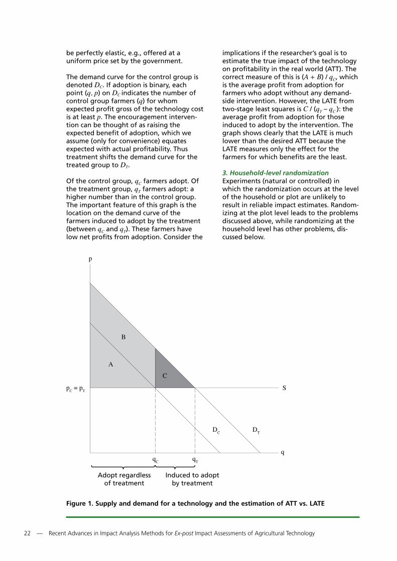
22 — Recent Advances in Impact Analysis Methods for Ex-post Impact Assessments of Agricultural Technology
be perfectly elastic, e.g., offered at a uniform price set by the government.
The demand curve for the control group is denoted DC. If adoption is binary, each point (q, p) on DC indicates the number of control group farmers (q) for whom expected profit gross of the technology cost is at least p. The encouragement interven-tion can be thought of as raising the expected benefit of adoption, which we assume (only for convenience) equates expected with actual profitability. Thus treatment shifts the demand curve for the treated group to DT.
Of the control group, qC farmers adopt. Of the treatment group, qT farmers adopt: a higher number than in the control group. The important feature of this graph is the location on the demand curve of the farmers induced to adopt by the treatment (between qC and qT). These farmers have low net profits from adoption. Consider the
implications if the researcher’s goal is to estimate the true impact of the technology on profitability in the real world (ATT). The correct measure of this is (A + B) / qC, which is the average profit from adoption for farmers who adopt without any demand-side intervention. However, the LATE from two-stage least squares is C / (qT – qC ): the average profit from adoption for those induced to adopt by the intervention. The graph shows clearly that the LATE is much lower than the desired ATT because the LATE measures only the effect for the farmers for which benefits are the least.
3. Household-level randomizationExperiments (natural or controlled) in which the randomization occurs at the level of the household or plot are unlikely to result in reliable impact estimates. Random-izing at the plot level leads to the problems discussed above, while randomizing at the household level has other problems, dis-cussed below.
Figure 1. Supply and demand for a technology and the estimation of ATT vs. LATE
p
pC = pT
qC
A
B
C
S
DTDC
qT
q
Adopt regardless of treatment
Induced to adopt by treatment

Recent Advances in Impact Analysis Methods for Ex-post Impact Assessments of Agricultural Technology — 23
The most serious issue with randomizing over households (instead of over villages, for example) is that adoption by some in the treated group will probably affect the outcomes of the control group. Such spill-overs invalidate comparisons between treated and control groups as a basis for es-timating the effect of a new technology. Sections 3.4 and 4.5 explain the problem of spillovers and how they affect current selec-tion on observables approaches. The problems described in the latter section carry over even to otherwise well-planned RCTs where randomization of technology over households is explicit.
To illustrate, we return to the example of tube wells in section 4.4. Suppose that instead of comparing adopters and non-adopters on observables, an RCT took place at the time the technology was introduced. A group of farmers was selected for treat-ment in which they were visited by exten-sion agents, told about the new technol-ogy, and offered the necessary materials for sale. The control group was not visited. Baseline data were taken before any adoption and then a follow-up took place two years later to see how farm profitabil-ity and household consumption had changed.
Randomization does not solve any of the spillover problems discussed in the selection on observables case: wage effects, local price effects, mutual insurance effects, and usage of the wells by non-adopters. Any of these could be serious enough to limit the validity of the experiment. Spillovers within the village are a consequence of adoption itself, not the research design being used. They will exist regardless of the researcher’s approach.
A further issue with randomization at the household level is that, in many cases, farmers in the control group may gain access to the new technology and choose to adopt it even when it is not offered to them, a problem often referred to as con-tamination of the control group. This is par-ticularly likely if the new technology is a farming technique rather than a physical input that is purchased. Adoption by control farmers is a problem because the estimated LATE no longer gives the effect for those who were induced to adopt by
the offer of the technology compared with those who would have adopted if given the treatment. Instead it measures the effect for those induced to adopt compared with a mixture of adopting and non-adopting households. Dropping the adopting house-holds in the control group from the sample prior to analysis does not fix the problem, because these may have indeed been the farmers that correspond to the adopters in the treated group. In this case, the treated adopters would be compared with control farmers who would never adopt, and this is the wrong counterfactual group for esti-mating the LATE.
5.3 Specific suggestions
Having cautioned against several potential new approaches for impact analysis, this section presents suggestions for future work. The main purpose of these sugges-tions is to help in clearly identifying a coun-terfactual group against which to compare adopters, accounting for inevitable spill-overs from adoption, and limiting contami-nation of the control group.
1. Use natural or randomized experiments where the village, community, or other appropriate social grouping is the unit of randomizationBy ‘natural’ experiment we mean a situa-tion in which assignment of the treatment is as good as random, possibly conditional on some observable variables, but that no specific attempt was made to randomize the treatment as in an RCT. The rollout of a technology over time and space might con-stitute a natural experiment in some cases. Using natural or randomized experiments in which the village, community, or other appropriate social grouping is the unit of randomization addresses the issue of spill-overs, not by ignoring them or trying to create an environment in which they do not exist, but rather by acknowledging that they are potentially important results of adoption and incorporating them into the measured effect of the new technol-ogy. Randomizing at a level higher than that of the household in the presence of spillovers has recently become standard practice among development economists. In the field of health, for example, Miguel and Kremer (2004) randomize drug treat-ment at the school level and Cohen and

24 — Recent Advances in Impact Analysis Methods for Ex-post Impact Assessments of Agricultural Technology
Dupas (2010) randomize mosquito net prices at the clinic level. In education, Muralidharan and Sundararaman (2009) and Kremer et al. (2009) randomize teacher and student incentives (respectively) at the school level.
When randomization takes place at the village level (as an example used for conve-nience, since this discussion applies also to other levels of randomization) in an RCT, two-stage least squares can be performed using households as the unit of analysis, provided that the standard errors are clus-tered at the village level.11 Clustering typi-cally causes standard errors to be much greater and requires many villages to be included in the experiment, which increases the cost and scale of the project. While this is an unfortunate consequence, the alterna-tive of household-level randomization gives a (potentially seriously) biased estimate of the effect of the new technology.
When randomization takes place at the village level and individuals are used as the unit of observation, regressing the outcome of interest on treatment status gives the average effect of the treatment being offered, regardless of whether the treat-ment induces adoption. This is known as the intention to treat effect (ITT). The ITT is a useful quantity because it gives the average impact of the treatment per house-hold regardless of adoption status, which can be used as a measure of the effective-ness of the treatment. The ITT accounts for all effects of the technology, both directly through adoption and through spillover effects on adopters and non-adopters.
The LATE scales the ITT by the fraction of adopters, so it measures the effect of adoption per adopter. Because the LATE is just the scaled ITT, it still includes the effect of spillovers. Provided that the treatment induces adoption for all farmers who would adopt under real-world conditions, while not inducing adoption for real-world non-adopters, the LATE gives the desired quantity for impact analysis of a technol-ogy: the ATT plus the average spillover effect per adopter.
In the case of an RCT, clustered randomiza-tion also ameliorates, to some extent, the ethical dilemma presented by Maredia
(2009), in which some farmers are offered a technology while it is withheld from others in the same village. Withholding treatment from some villages is a less artificial act than withholding it from households, as the number of treated villages is likely to be determined by budget constraints and treating any of the control villages is unfea-sible. Of course, data collection must still take place in the control villages, and if the marginal cost of distributing the technol-ogy during surveying is low, then the artifi-cial withholding of treatment will present an issue.
A further benefit from including many villages in an evaluation is that the effect of the technology is estimated using several geographically distinct locales. This adds a degree of external validity to the results, since the estimates will be based on the results of adoption across locations with po-tentially heterogeneous effects from adoption. For example, if the new technol-ogy is useful only when rainfall is scarce (such as a drought-resistant seed variety), then measuring the effects of adoption only in a village that experiences plentiful rain will not reveal the true returns of adoption. A study covering many villages, however, could observe a range of rainfall levels and obtain an estimated effect closer to the true quantity.
2. Use supply-side interventions where the new technology is introduced to entire villagesVillage-level clustering is not sufficient to recover the desired (ATT + average spill-over) estimate because it does not ensure that adoption due to the treatment corre-sponds to those who would take up the technology under true market conditions. For this reason, the treatment should simulate the introduction of the new tech-nology on the market as closely as possible. The simplest example of this in the setting of an RCT is to choose a set of villages that do not have the technology and to randomly choose a subset of villages in which to sell the technology at the ‘market price’. Adopters will then be the entire set of farmers who find it optimal to adopt when the technology is available for purchase, i.e., those who would purchase under real-world conditions. The LATE is as desired: the effect of the technology, (ATT +

Recent Advances in Impact Analysis Methods for Ex-post Impact Assessments of Agricultural Technology — 25
average spillover), when the technology is made available for sale.
It is important to note that not all supply-side interventions yield the correct LATE. If the product is already available in villages and the intervention is a subsidy to sellers that shifts supply of the technology outward, then the analysis suffers from problems similar to those discussed for de-mand-side treatments. Only the effect on marginal adopters is estimated. Thus it is important for the supply-side intervention to be a relaxation of a supply constraint so that villages with no access to the technol-ogy are given access at market prices.
3. Do not limit research designs to RCTs. Natural experiments can yield reliable estimates of impact even in the absence of controlled, explicit randomizationThere are situations in which an RCT is a plausible option that should be pursued. If a new technology must be rolled out over time due to supply constraints, randomizing the villages receiving the technology at each phase of the rollout may be a simple and feasible task that provides precisely the supply-side RCT necessary for estimating impact. This can be done by matching pairs of villages based on observables, then randomly drawing treatment within each pair. Care must be taken not to ‘sabotage’ the technology by introducing it to areas in which it is unlikely to be taken up, since such a strategy could damage the reputa-tion of the technology and inhibit its suc-cessful expansion.
In other cases, it is not possible to plan and carry out an RCT. While there may be op-portunities for good impact analysis, some creativity is required. Rollouts of a technol-ogy that were arguably random, even when they were not explicitly randomized, can be analyzed in a similar way to those of RCTs. The assumption of randomness in the rollout cannot be fully tested, so it is impor-tant that researchers with institutional knowledge of the technology and its rollout process provide guidance on how the rollout occurred. In other cases, the rollout follows explicit rules based on ob-servables that can be used to instrument treatment. Provided that the necessary data are available, treating the rollout process as a natural experiment allows for the analysis
of technologies that have already been diffused. It often allows for use of very large administrative databases. This is a distinct advantage over RCTs, which are only possible for new technologies.
Other kinds of natural experiments may be usable as well. A geographic discontinuity approach may be possible when a specific area is chosen for diffusion of the technol-ogy. Provided that the boundary defining which farmers receive the technology is not physically or politically important (such that villages on either side of the boundary are very different from each other), the two groups of villages can be compared, with the status of being on the ‘diffusion side’ of the boundary used as the indicator of treat-ment. The natural experiment is that, since the boundary is assumed to be arbitrary, the side on which the villages lie is essen-tially random. Regression discontinuity methods might be applied in order to account for differences between the two sides of the boundary due to continuous changes in village characteristics over space.12 However, here again, we measure only local treatment effects in the proximity of the discontinuity rule.
An example in which a boundary disconti-nuity design might be successful is the in-troduction of technologies that control Striga hermonthica, a parasitic weed that has spread widely throughout Africa, sup-pressing yields of maize and other grains in affected areas (Berner et al., 1994). Striga is spread by wind, livestock droppings, and sale of contaminated seed at markets. There may be a geographical frontier between areas that are infested and those that have yet to be affected, with the frontier advancing from year to year. Suppose that researchers map the infesta-tion frontier and collect baseline data on crop yields (and other outcomes), prior to the introduction of a new striga control technology (whether chemical or biological) for sale to farmers.
Figure 2 gives a stylized illustration of the geographic discontinuity design that could be used in this context. The ‘T’ villages are those affected by striga where the new technology is offered for sale. The ‘U’ villages are unaffected because the infesta-tion has yet to reach them. The boxed ‘U’

26 — Recent Advances in Impact Analysis Methods for Ex-post Impact Assessments of Agricultural Technology
and ‘T’ villages form the treatment and control groups under consideration, because they are sufficiently close to the boundary to make them comparable along all dimensions except for their exposure to striga.
The effect of the technology can be esti-mated by a DD method that uses introduc-tion of the technology as an instrument for adoption, then compares the change in yield for the baseline-infested (treated) areas to the baseline-uninfested areas (control). The intuition is that in the absence of infestation, changes in yield over time between the treatment and control villages would be similar. Then the DD estimator recovers the average change in yield due to adoption, because the unin-fested area is an appropriate counterfac-tual. Note that while no randomization of treatment is necessary for this evaluation, it is necessary to have baseline data for both treatment and control areas, as well as follow-up data after adoption has occurred.
Needless to say, the list of possible research designs is longer than: i) RCTs; ii) arguably / ‘as-good-as’ random rollouts; and iii) geo-graphic discontinuities. The key is to be creative when defining sources of random variation in supply of the new technology.
Such unique research designs will be case-specific and will require intimate knowl-edge of the technology’s introduction and subsequent diffusion. Brainstorming involv-ing economists as well as staff involved in the technology’s development and release will help identify suitable options.
Whether use of PSM survives as a viable strategy depends on the details of the tech-nology diffusion process. The only situation in which PSM is obviously suitable is when availability of the technology in villages is as good as random after conditioning on observable characteristics of the village. This does not seem likely, but if the re-searcher can justify such an assumption, PSM could be a useful approach.
4. Leverage public–private–civil society partnerships to perform supply-side interventionsThe most likely best case for RCT is the random introduction of a new technology into villages. A potentially attractive means for doing this is to pursue partnerships between the originator of the technology and organizations that are already on the ground distributing the technology, whether they are private dealers or NGOs. In the case of seeds, partnerships with local agro-dealers could provide a fruitful col-
Figure 2. Stylized illustration of a geographic discontinuity design
U
T
UU
UU
U U
U
U
U
U
TT
T
T
T
TT
T
T
T
T
T: treatedU: untreated
in sample
boundary of infestation

Recent Advances in Impact Analysis Methods for Ex-post Impact Assessments of Agricultural Technology — 27
laboration for introducing new varieties to selected areas. Local agro-dealers already provide agricultural inputs to villages and so provide a natural channel for distribut-ing new varieties.
An RCT including agro-dealers in the supply chain would need to do two things with respect to distribution of the new seed variety. Firstly, it would have to make the new variety available to a random subset of dealers. Secondly, it would have to provide adequate incentives for dealers to actually buy the seeds and offer them for sale to farmers in their territories. The former should be simple in most cases, since agro-dealers already form part of the supply chain. The latter might be accomplished by subsidizing the wholesale price of seeds to dealers.
An advantage of releasing the new technol-ogy through agro-dealers is that farmers are already used to buying from them and will have some confidence that supply will remain available in the future (as opposed to obviously randomized interventions where it is unclear whether the new tech-nology will continue to be offered for sale in the future). In addition, prices are set ac-cording to market forces because the dealer has a profit motive. This makes observed adoption more reliable than interventions that push new technologies by methods outside of the traditional supply chain. After all, once the rollout is complete, regardless of the method, it is likely that dealers will be
the only sustainable suppliers. Incorporating them into the process at the evaluation phase is a natural way to accurately estimate the effects of the new technology.
5. Plan the evaluation before and conduct it during diffusion of a new technologyThe fact that impact analyses are referred to as ex-post does not suggest that they should be planned and performed after the fact, a point made clearly in Maredia (2009). Baseline surveys that reflect pre-adoption outcomes accurately must be un-dertaken prior to diffusion, and these may take some time to carry out. It goes without saying that an RCT requires advanced planning prior to rollout of the technology, but even if the rollout is not explicitly ran-domized, any follow-up surveys taking place during the rollout must be ready for administration.
Failing to plan the evaluation ahead of time has multiple negative consequences. The first is that it may result in a lack of appro-priate baseline data on the pre-adoption characteristics of farmers and villages. The second is that the researcher may miss a chance to implement a clear research design. The last is more subtle and relates to the temptation to evaluate the technologies that are perceived to have been already suc-cessful. By planning and executing impact analyses for all projects, even those that are not perceived to be successes, it is possible to obtain a better picture of the returns to the entire portfolio of projects.

28 — Recent Advances in Impact Analysis Methods for Ex-post Impact Assessments of Agricultural Technology
The goal of this section is to give concrete examples of impact analyses that could be un-dertaken using the methods discussed. Each example is based on a new technology devel-oped in collaboration with a CGIAR research center and each proposes a way to evaluate impact as the technology is rolled out. It should be noted that these proposals are for new technologies that have yet to be completely diffused. This is not a coincidence: the best ap-plications are those for which evaluations take place as the technology is rolling out.
6.1 Genetically improved farmed tilapia
The Worldfish Center, along with other or-ganizations, has spent decades developing genetically improved farmed tilapia (GIFT) through selective breeding programs. The fish ‘seed’ is distributed through public–private partnerships in many countries, mostly in Southeast Asia. Adoption has been most successful in the Philippines and Thailand. Distribution in Bangladesh has been logistically difficult, resulting in very little adoption. Adoption in Vietnam has had some success, but there appears to be room for more growth.
Previous impact evaluation, summarized in an Asian Development Bank report (Opera-tions Evaluation Department, 2005), has relied mostly on research station and on-farm evaluations of differences in yield (weight at harvest) and surveys of fish farmers for information on profitability. The report states that the yield numbers are controversial, highly debated, and not care-fully peer-reviewed.
Because the ADB report mentions explicitly that there have been supply-side con-straints in Bangladesh, an RCT may be ap-propriate for assessing the impact of GIFT on such outcomes as yield, income, farm profits, and poverty. While the estimated impacts would be specific to Bangladesh, the results may be applicable to some extent to countries where diffusion has already been successful. The first step of the evaluation would be to identify a random
subset of villages or communities that are engaged in tilapia farming and randomize them into treatment and control groups. Then a baseline survey of household and farm characteristics would be conducted.
If public–private partnerships are viable in Bangladesh, aquaculture suppliers and dealers in or near villages selected for treat-ment would be offered the GIFT seed and monetary incentives to sell the new variety. This would both make supply available to dealers and ensure that they actually offer the GIFT for sale so that farmers have a chance to adopt it. If private partnerships are not feasible but NGO or governmental in-volvement is strong, these groups could offer extension services that sell GIFT in the treated villages. Control villages would experience no changes. After a period of time long enough for farmers to purchase, use, and realize the benefits and costs of the new variety, a fol-low-up survey would be conducted.
For the empirical analysis, the dependent variable would be the change in outcome (yield, income, profit, consumption, etc.) between baseline and follow-up surveys. The variable of interest – adoption of the GIFT variety – would be instrumented by a variable equal to 1 if the village was offered GIFT seed and 0 if the village was a control. The estimated coefficient on adoption would then give the effect of adoption on adopters (ATT), plus any spill-overs induced by adoption.
It is not clear (to the authors) how much learning-by-doing there is in tilapia farming or how fast adoption would take place. If these are thought to be important factors, then follow-up surveys could take place over successive years to estimate the path of adoption and outcomes over time, but only if the control group did not obtain the GIFT technology in the meantime.
6.2 Treatment for internal parasites in goats
During the past decade, the Australian Centre for International Agricultural
6. Examples of approaches to evaluation

Recent Advances in Impact Analysis Methods for Ex-post Impact Assessments of Agricultural Technology — 29
Research (ACIAR) and the International Livestock Research Institute (ILRI), among others, have conducted a program to educate Filipino farmers about the serious problem of parasites in goats, and to help them introduce strategies for preventing mortality from parasites. The work is docu-mented in a report by ACIAR (Montes et al., 2008). After researching optimal procedures and technologies for preventing and com-bating parasites, they performed outreach activities in the form of intensive farmer livestock schools funded by national and local governments. Farmers invested their time and effort in class learning as well as investing in de-worming drugs and making on-farm improvements. The focus was on non-chemical means of control, partly because drug-resistant worms are becoming a serious problem.
Previous impact analysis has attempted to estimate the ATT through a case study with very few animals. This ATT does not neces-sarily reflect the impact of the methods because it is not clear that it represents the outcomes under actual ranching behavior. These benefits were then projected onto the population by using the estimated adoption rate in the regions included in the program.
The technology being evaluated is a package of livestock management tech-niques taught by the schools. A simple impact evaluation of this technology would select a group of villages or communities where goats are raised, then randomly offer field school classes to a subset of them. This should be done only in parts of the country that have not yet been exposed to the schools, since the program took place initially in two regions but would be suitable for other areas of the country as well. After the classes conclude and suffi-cient time has passed for farmers to fully implement their new techniques, follow-up data could be collected on farm-level outcomes.
An analysis that randomly offers classes in new regions would have two effects of interest. First is the reduced form effective-ness of the schools themselves in changing outcomes. This can be obtained by regress-ing outcomes of interest (profitability, herd mortality, etc.) on the presence of a field
school. The second effect of interest is from an instrumental variable (IV) regression using the school’s presence as an instru-ment for farmers’ adoption of the new techniques.
An obvious concern with this approach is the potential for spillover of knowledge between communities where the schools are offered and those where they are not. The seriousness of this problem depends on the geographical distance between the communities and the degree of interaction between them. It does not seem that the spread of parasites between farmers’ herds is an important issue. Even in the presence of spillovers of this sort, an RCT would still be useful. If there is no spillover, then the IV regression yields the pure ATT of the new techniques, while if there are spill-overs, the IV regression gives the ATT plus the impact of the spillovers from adoption.
6.3 Drought-tolerant maize varieties
The Drought Tolerant Maize for Africa (DTMA) Project13 is a major ongoing effort conducted by the International Maize and Wheat Improvement Center (CIMMYT) and the International Institute for Tropical Agri-culture (IITA). The project claims that the gains from introduction of drought-toler-ant varieties will lead to yield advantages of up to 34% over improved but non-drought-tolerant varieties (La Rovere et al., 2010), with up to 50% advantage during drought seasons. This is an ex-ante estimate from field trials, so it is important to evaluate such claims under real-world adoption as the program progresses and diffusion takes place.
A straightforward RCT supplying new seed varieties to a random subset of agro-dealers could be used for such an evaluation. Indeed, given that the project is still at a relatively early stage and supply is still severely constrained, this could prove to be an excellent candidate for an RCT evalua-tion. An additional approach may also be useful, and this is illustrated here as an example of using a natural experiment for the evaluation of technologies.
Drought tolerance is a risk-reducing tech-nology designed to limit yield losses in times of drought rather than increase yields
30 — Recent Advances in Impact Analysis Methods for Ex-post Impact Assessments of Agricultural Technology
in times of adequate rainfall. As discussed in section 2.1, evaluating this technology requires that drought actually occurs for some of the farmers involved in the evalua-tion. Our suggested approach is to compare adopters in areas with equal levels of drought risk, but where some experienced drought and others did not. A DD estimator that controls for ex-ante drought risk can be used to obtain estimates of the yield effects (and other outcomes) for actual adopters. In this case, the randomization required for identification in a natural ex-periment comes from rainfall shocks.
The first step of this evaluation would be to perform a baseline survey on areas where adoption of drought-tolerant varieties is likely to be high when they become avail-able on the market. A follow-up survey would then be conducted on the same farmers once sufficient time has passed for substantial adoption to occur. Researchers would then identify the subsample of farmers who had adopted the new drought-tolerant varieties made available by DTMA. The sample should include farmers within a similar agro-ecological zone (although the evaluation could include comparisons within several zones), but who are spread far enough apart to provide variation in realized rainfall and drought. The sample would then be further limited to adopting farmers who experi-enced drought at baseline. This is an impor-tant requirement for identifying the effect of the drought-tolerant varieties.
The next step would be to compile fine-grained historical rainfall data for the areas in the sample. This data would be used to estimate the drought risk for each farmer in the dataset.
The econometric strategy is to compare adopters with similar levels of drought risk but who had different realized drought outcomes. This can be done either with ordinary least squares (OLS) regression or with PSM. Indeed, this is a good example of the proper use of PSM, since matching between farmers that were affected by drought and those that were not would take place on the estimated probability of drought. The key assumption to make this analysis valid is that risk of drought is random after conditioning on our con-
structed measure of predicted drought. After matching farmers on the basis of drought risk, the DD estimator can be used to see how the change in yield over baseline differed by drought status. The average of this difference is the yield ad-vantage of the technology under drought conditions.
This estimate can then be multiplied by the average probability of drought to obtain the expected annual yield gain from adoption for adopters. A similar method could then be used to estimate impacts for profits, income, and poverty status, provided that sufficient data were collect-ed. Adoption effects could then be disag-gregated on the basis of drought risk. The effect for farmers at relatively low drought risk might be compared with those at high risk to see if the realized gains during drought seasons are the same. Stratifying the matching on such other household characteristics as gender of household head or education level could give effects for dif-ferent subpopulations, providing a richer view of the distribution of the technology’s impacts.
There are important caveats to this research approach. Adopting the technology and lowering drought vulnerability for maize may lead farmers to re-optimize their pro-duction plan and farm activities, which could include the planting of more risky crops since their maize production risk has fallen. Since adopting farmers experiencing drought and those not experiencing drought will have engaged equally in this re-optimization, such an effect would not be identified by looking at differences between the two groups of adopters. Simi-larly, if the drought-tolerant variety has an improved yield even in times of good rainfall, this change cannot be identified separately from the time trend in yields for adopters. The estimated adoption effect here would indicate only by how much the adoption of drought-tolerant varieties alters the drought to no drought spread in outcomes. Changes in production behaviors and good-weather yield could be examined casually by comparing changes in crop com-position and labor supply for adopters with those of non-adopters using DD, but the validity of this analysis would depend on the assumption that in the absence of

Recent Advances in Impact Analysis Methods for Ex-post Impact Assessments of Agricultural Technology — 31
drought-tolerant adoption, the adopters and non-adopters would have changed these choice variables in the same way and that yield trends for the non-drought-toler-ant variety were similar between adopters and non-adopters.
The key aspect of this example, and what makes a natural experiment feasible, is that
rainfall and drought are basically random after conditioning on the past history of rainfall. The fact that the technology’s benefits are activated randomly allows adopters to be compared with other adopters. The key here is that we are not matching on the basis of a choice variable, but rather on an arguably exogenous variable in the form of drought risk.

32 — Recent Advances in Impact Analysis Methods for Ex-post Impact Assessments of Agricultural Technology
7.1 The challenge of estimating long-term and aggregate effects
The econometric methods discussed so far can be used to establish the impact of tech-nology adoption on outcomes at the producer level. These outcomes can be of dif-ferent types (yield on the plot, production on the farm, welfare of the household, or labor demand), but in all cases impact is being measured on the units of observation used in the statistical analysis (similar methods can be used to measure impact at the consumer level, on health for example). The units could be villages, but will never be much bigger since statistical analysis requires a very large number of observations. In addition, such impact can be measured only when technol-ogy diffusion is incomplete and it is possible to find counterfactuals that are unaffected by the technology. Therefore, impact analyses can be conducted only before sector-wide or economy-wide effects have taken place, if the implementation or even the data collection requires some design.
On the other hand, we are often interested in measuring ex-post the aggregate benefit of a technology that has diffused over large areas. In this case, the overall impact of the technology should capture the changes that occurred in aggregate supply, demand, and price in the sector. If the sector is large enough, with spillovers into input markets, employment, and income effects, the impact analysis should also include general equilib-rium effects. There is, of course, no counter-factual situation that can be observed, and hence researchers will resort to different types of analyses. One is to focus on smaller units of observation (such as villages) on the presumption that markets are not well inte-grated, so each unit represents a small ‘economy’; and to rely on econometric analysis of the observations over time to identify the causal effect of uneven develop-ment of technological change on these units. The second type of analysis is to resort to simulation models to extrapolate impacts measured at the micro level (most often in-creases in yields) to the level of aggregate effects.
7.2 Estimating the effects of technological change with long panel data
This is best illustrated by Foster and Rosenz-weig’s body of work on the effects of the Green Revolution in India (Foster and Rosenzweig, 1996; 2003; and 2004). Starting in the mid-1960s with the introduction of new hybrid seed varieties, the Green Revo-lution led to significant improvements in crop yields over a long period of time. An important aspect of the Green Revolution experience is that it progressed at a differ-ent speed in different parts of the country, creating the opportunity to analyze its effects in a panel setup. A simplified model that captures the essence of the methodol-ogy for measuring the impact of yield im-provement on household or village level outcomes is written as:
Yivt = βyieldvt + Xivtγ + μi + vt + εivt
Yvt = βyieldvt + Xvtγ + μv + vt + εvt
where Yivt (Yvt) are outcomes of interest at the household (village) level, yield is an index of yield at the village level, X are control variables, μi (μv) are fixed household (village) effects, vt fixed time effects, and ε error terms. The yield index is a Laspeyres index of village level yield on irrigated HYV crops. Foster and Rosenzweig use a panel of about 4,000 households from 250 villages with three rounds of observations (in 1971, 1982, and 1999).
With spatial and temporal fixed effects, identification of the impacts of an increase in yield comes from the differential change in yields across villages. In some specifications, the time-fixed effect is State-specific, focusing the identification on the differential pace of yield improvements across villages within a State. Outcomes of interest are, for example, agricultural income, non-farm income, or total income at the household level; and rural wage, non-farm employ-ment, total income, or poverty at the village level.
7. Long-term and aggregate effects

Recent Advances in Impact Analysis Methods for Ex-post Impact Assessments of Agricultural Technology — 33
A couple of issues are worth noting:1. The yield index used in the equation is
affected by more than just technological change. This is because it results not only from technological change but also from changes in productive inputs such as fertilizer, labor, or education, all possibly influenced by technological change, but also by other factors. So there may be some concern that changes in the yield index at the village level capture the other factors that are correlated but not due to technology change. To circumvent this problem, Foster and Rosenzweig (1996 and 2003) recover a district-year specific technology factor from estimation of a farm-level profit function, and then instrument yield with this technology factor and some village characteristics.
2. The estimation measures the effects of relative changes in yields across villages, but not the nationwide or State-level aggregate effects of technology change. For example, the extent to which the Green Revolution brought about a large decline in prices over the whole of India, thereby reducing poverty, is captured by the time-fixed effects and not attributed to the changes in yield.
Still, this approach goes a long way towards understanding the aggregate and long-term impacts of a large technological change such as that embedded in the Green Revolution. Note, however, that the analysis is very demanding in terms of data, as it requires a sufficiently large sample of ob-servations to be representative of the ag-gregate area of concern, over a long period of time that covers the technology diffusion period, and detailed farm data that allow for extracting the role of technological change from observed yields.
7.3 Extrapolating micro results with partial equilibrium simulation models A second type of analysis uses simulation models. These translate or extrapolate the (estimated/measured) microeconomic effects into some aggregate number, based on assumptions about the sector or the
economy at large. They rely on functional form assumptions, assumptions on supply and demand elasticities, and strong as-sumptions on the functioning of the markets. Hence, in no way can these models be considered to estimate an aggregate impact in the same sense as econometric methods. On the other hand, they are a powerful way of translating micro-level es-timations into plausible orders of magni-tude of macro effects, if done with care and with sufficient sensitivity analysis.
The most common of these simulation models is the economic surplus approach, based on a partial equilibrium model of the sector in which the technological change has occurred. The idea is that technological change induces a shift in the supply curve, which in turn induces a decline in price and a new equilibrium on the market. The economic surplus is calculated as:
ES = pqk ( 1 + )
where p and q are the initial price and quantity of the commodity of interest, k is the proportional shift in the supply curve induced by technology change, and εs and εd are the supply and demand elasticities.
The key input to this simulation is of course the k factor, i.e., the direct effect of techno-logical change on the supply curve. The factors that allow the extrapolation from k to the value of the economic surplus are the observed total output and price, and the assumed elasticities (usually drawn from some other studies).
The k factor is determined by the combina-tion of changes in yield and costs. Pictured on a supply curve, changes in yield are hori-zontal shifts, while cost reductions are vertical shifts, which can be made equiva-lent to proportional yield changes with the supply elasticity. Most studies focus on in-creases in yields. Changes in yields them-selves are drawn from either field trials or observational differences in yields between crop varieties. Neither is very satisfactory. What is needed is an estimated supply shift or yield increase that can be causally attrib-uted to technological change. Hence the challenge is as described in section 7.2 on estimating the impact of technology on yield.
1 k2 εs + εd

34 — Recent Advances in Impact Analysis Methods for Ex-post Impact Assessments of Agricultural Technology
This method has been used extensively in ex-post studies, computing time series of economic surplus based on observed output and prices, and assumed elasticities, and then aggregating the results over years to compute the aggregate effect. In many of these studies, the principal effort has been to measure the area (and output) affected by the specific technological change of interest, notably the development of certain varieties by the CGIAR (Byerlee and Traxler, 1995). Some studies run sensitivity analyses to the assumed elasticities. The method is also used in ex-ante studies, based on field trials for specific varieties (see Falck-Zepeda et al., 2007).
7.4 Poverty simulation
A further step in applying a ‘poverty elastic-ity’ to the calculated aggregate production increase or welfare effect to obtain an impact on poverty has been taken (Fan et al., 2005; Alene et al., 2009). The key question of course is how the poverty elas-ticity has been estimated and whether or not it applies to this specific context. Obvi-ously, the poverty effects of an increase in aggregate welfare depend on who benefit-ed from the increase in economic surplus among large producers, small producers, urban consumers, etc., and what their initial poverty levels were. So it seems a bit of a stretch to conduct a simulation exercise by applying a poverty elasticity estimated in a different context to an aggregate increase in production. Poverty impact should be ad-dressed with rigorous econometric analyses like those discussed in section 7.2.
In conclusion, the validity and usefulness of these simulations is nothing less than the validity of the elements that enter into the simulations. It is therefore critically impor-tant that the k factor is estimated rigorous-ly, that sensitivity analyses are made on the elasticities in the economic surplus simula-tions, and that it is clear that these are useful simulations as opposed to impact estimations.
7.5 Computing aggregate impacts with general equilibrium simulation models Going beyond the sector model discussed in the previous section, researchers have used
general equilibrium models for cases where the change in technology is sufficiently large to induce effects on trade and on output and input markets that, in turn, may induce spillover effects on other sectors (Arndt et al., 1999; Dorosh and Thurlow, 2009; Diao et al., 2010). The most commonly used type is the computable general equilibrium (CGE), a model in which supply and demand in all markets is balanced with endogenous prices, although a few studies use the social-accounting matrix (SAM) multiplier approach, a Keynesian demand-driven general equilib-rium model with excess supply in all markets.
CGEs essentially represent a system of markets that reach equilibrium through prices. Very broadly speaking, they consist of: (i) supply functions for each sector of the economy, derived from production models that are usually some combination of a constant elasticity of substitution (CES) ag-gregate in primary factors of production and Leontief technology for intermediate inputs; (ii) demand functions emanating from households (using some standard demand system); and (iii) markets that balance either with flexible prices or with quantity adjust-ments according to tradability.
CGEs were developed initially for the modeling of trade and they remain stron-gest in this area. Foreign goods and domestic goods are imperfect substitutes (using CES and constant elasticity of trans-formation or CET functions), which also lead to specific demands for imports and supplies of exports in response to the relative prices of foreign and domestic goods. The rest of the model includes gov-ernment and institutions that tax or transfer, mostly with fixed shares (e.g., the return to labor or to capital in each sector is allocated in fixed proportions across house-holds, etc.). Sectors thus compete through their interactions in the input and factor markets. The data needed for such models essentially provide a static picture of all the flows in one particular year (the SAM derived from national income accounts and an input–output matrix) from which all shares are derived and which have four sets of elasticities: (i) elasticity of substitution between factors in the production function; (ii) demand elasticities (or more specifically

Recent Advances in Impact Analysis Methods for Ex-post Impact Assessments of Agricultural Technology — 35
the parameters of a consistent demand system) for households; (iii) elasticity of sub-stitution between imported and domestic goods; and (iv) elasticity of transformation between commodities for the domestic markets and exports for each sector.
CGEs can have different levels of disaggre-gation (e.g., number of sectors, number of household types) and, because elasticities are rarely estimated and most often ‘guessed’, there is a difficult tradeoff between gaining details in shares and having to rely on an increasing number of assumed elasticities. Most CGEs are static models, although some have introduced the updating of capital stocks, labor supply, and possibly technological factors that make them sequentially dynamic. However, an additional set of assumptions is needed for these ‘updatings’. Some models attempt to capture the particularity of self-con-sumption (Arndt et al., 1999), or link micro-simulations applying the results obtained in CGEs to individual households and, by this, to obtain a better measure for poverty effects (Diao et al., 2010).
CGEs have the advantages of a consistency framework that forces markets and budgets to balance, and an anchoring of all simulat-ed effects on the observed initial relative sizes of sectors and commodities. However,
the extent of these models’ assumptions (in terms of market functions, representation of agents that make choices, existence of trans-actions costs and constraints, heterogeneity across producers, etc.) makes them more suitable for discussion of alternative broad policy choices than for actual predictions of the effect of such specific shocks as techno-logical change. The paper by de Janvry and Sadoulet (2002) uses archetype CGEs to illus-trate the different channels through which an agricultural technological change can affect the rest of the economy. Although widely cited, this paper only intends to illus-trate the different channels incorporated in a CGE, and to show how their relative im-portance varies with the relative structural features of economies, the degree of openness of the economy, the substitutabil-ity between foreign and domestic goods, and the functioning of markets. Stark con-trasts can then be shown to exist in the impacts of the same technological change across archetypes that represent a South Asian or a sub-Saharan economy. Sensitivity analysis shows qualitative results to be robust, but quantitative results cannot be taken too seriously. In the application of focus of this paper – measuring the impact of a technological change – CGE simulations can basically help track, under a set of strong assumptions, the economy-wide effects of that particular change.

36 — Recent Advances in Impact Analysis Methods for Ex-post Impact Assessments of Agricultural Technology
Endnotes
1 Examples of this type of analysis include Fan et al. (2000), Evenson and Gollin (2003), Raitzer and Kelley (2008), Maredia and Raitzer (2010), and Alston et al. (2000).
2 This paper does not specifically address issues concerning CGIAR research on best practice or policy.
3 As Gollin (2010) says, “the current generation of improved varieties is not so easily identified. Nowadays, we are often trying to distinguish between one generation of improved varieties and a previous generation. Are farmers growing the ‘old’ hybrid maize, or a ‘new’ hybrid maize? … It is not clear that farmers themselves can accurately tell you what varieties they are growing. Even where they purchase seed, the nature of seed systems in Africa is such that they may not know with any accuracy what variety they are growing”.
4 In the case where farmers engage in substantial subsistence consumption, implied profits can still be measured by treating own-consumption as a sale at local market prices, because this approximates the opportunity cost of own-consumption.
5 While there are such other interesting spillovers as economy-wide price effects and the effects of adoption by one farmer on the adoption decision-making of other farmers, this paper focuses only on spillovers that affect such microeconomic outcomes as income and profits.
6 Good examples of this work can be found in Adato and Meinzen-Dick (2007). We should point out that by ‘qualitative analysis’ we mean methods that are not data-driven in reaching their conclusions. There is some confusion on this point because in a quantitative analysis, binary variables (like poverty status) are often called ‘qualitative’ data. Using binary variables in a quantitative framework does not imply that the analysis is qualitative.
7 Bellon and Reeves (2002) collect a number of recent papers elaborating on on-farm trial methods and their comparison with research station trials.
8 Note the contrast between the objectives and methods of the agricultural scientist and the economist. The scientist wants to hold all factors constant between treatment and control plots, including all complementary inputs. The economist, on the other hand, most certainly does not want to hold all else constant, as the endogenous adjustments of inputs and management practices due to adoption are potentially important determinants of differences in outcomes between adopting and non-adopting farmers. Failing to adjust inputs and management practices to the new technology corresponds to measuring a sub-optimal use of the new technology from the farmer’s vantage point.
9 PSM methods are also common in studies that go beyond analysis of agricultural technologies, for example evaluations by the International Food Policy Research Institute (IFPRI) on community development projects (Nkonya et al., 2008) and farmer field schools (Davis et al., 2010).
10 Encouragement designs are common in medical research, e.g., Hirano et al. (2000). Bradlow (1998) gives a clear explanation of encouragement designs along with an application to marketing.
11 See Cameron and Trivedi (2005) for a technical but approachable review of clustered standard errors, which is beyond the scope of this paper.
12 Imbens and Lemieux (2008) provide a useful guide to regression discontinuity designs. An important caveat of all discontinuity designs is that they estimate the LATE for those close to the boundary, which might not be applicable far from the boundary.
13 For more information about DTMA, see http://dtma.cimmyt.org.

Recent Advances in Impact Analysis Methods for Ex-post Impact Assessments of Agricultural Technology — 37
References
Adato, M. and Meinzen-Dick, R. 2007. Agricultural Research, Livelihoods, and Poverty: Studies of Economic and Social Impacts in Six Countries. Johns Hopkins University Press: Baltimore, MD, USA.
Agricultural Technology Adoption Initiative. 2010. Barriers to the Adoption of Agricultural Technologies in Developing Countries. Draft white paper. http://atai.podconsulting.net/sites/default/files/documents/ATAI%20white%20paper%20062610.pdf. Version 2, June 2010.
Alene, A.D., Menkir, A., Ajala, S.O., Badu-Apraku, B., Olanrewaju, A.S., Manyong, V.M., and Ndiaye, A. 2009. The economic and poverty impacts of maize research in West and Central Africa. Agricultural Economics, 40(5): 535–550.
Alston, J.M., Chan-Kang, C., Marra, M.C., Pardey, P.G., and Wyatt, T.J. 2000. A Meta-Analysis of Rates of Return to Agricultural R&D. IFPRI Research Report no. 113. International Food Policy Research Institute: Washington, DC, USA.
Arndt, C., Jensen, H., Robinson, S., and Tarp, F. 1999. Marketing Margins and Agricultural Technology in Mozambique. IFPRI TMD Discussion Paper no. 43. International Food Policy Research Institute: Washington, DC, USA.
Bellon, M.R. and Reeves, J. (eds). 2002. Quantitative Analysis of Data from Participatory Methods in Plant Breeding. International Maize and Wheat Improvement Center: Mexico DF, Mexico.
Berner, D.K., Cardwell, K.F., Faturoti, B.O., Ikie, F.O., and Williams, O.A. 1994. Relative roles of wind, crop seeds, and cattle in dis-persal of Striga spp. Plant Disease, 78(4): 402–406.
Bradlow, E.T. 1998. Encouragement Designs: An approach to self-selected samples in an experimental design. Marketing Letters, 9(4): 383–391.
Byerlee, D. and Traxler, G. 1995. National and international wheat improvement research in the post-Green Revolution period: Evolution of impacts. American Journal of Agricultural Economics, 77: 268–278.
Cameron, A.C. and Trivedi P.K. 2005. Microeconometrics: Methods and Applications. Cambridge University Press: New York, NY, USA.
Catley, A., Abebe, D., Admassu, B., Bekele, G., Abera, B., Eshete, G., Rufael, T., and Haile, T. 2009. Impact of drought-related vaccination on livestock mortality in pasto-ralist areas of Ethiopia. Disasters, 33: 665–685.
Cochrane, W.W. 1979. The Development of American Agriculture: A Historical Analysis. University of Minnesota Press: Minneapolis, MN, USA.
Cohen, J. and Dupas, P. 2010. Free distribu-tion or cost-sharing? Evidence from a ran-domized malaria prevention experiment. Quarterly Journal of Economics, 75(1): 1–45.
Conley, T.G. and Udry, C.R. 2010. Learning about a new technology: Pineapple in Ghana. American Economic Review, 100(1): 35–69.
Davis, K., Nkonya, E., Kato, E., Mekonnen, D.A., Odendo, M., Miiro, R., and Nkuba, J. 2010. Impact of Farmer Field Schools on Agricultural Productivity and Poverty in East Africa. IFPRI Discussion Paper no. 00992, International Food Policy Research Institute: Washington, DC, USA.
de Janvry, A., and Sadoulet, E. 2002. World poverty and the role of agricultural tech-nology: Direct and indirect effects. Journal of Development Studies, 38(4): 1–26.
Dey, M.M., Paraguas, F.J., Kambewa, P., and Pemsl, D.E. 2010. The impact of integrated aquaculture-agriculture on small-scale farms in southern Malawi. Agricultural Economics, 41: 67–79.

38 — Recent Advances in Impact Analysis Methods for Ex-post Impact Assessments of Agricultural Technology
Diao, X., Nwafor, M., Alpuerto, V., Akramov, K., and Salau, S. 2010. Agricultural Growth and Investment Options for Poverty Reduction in Nigeria. IFPRI Discussion Paper no. 00954, International Food Policy Research Institute: Washington, DC, USA.
Dillon, A. (2008). Access to Irrigation and the Escape from Poverty: Evidence from Northern Mali. IFPRI Discussion Paper no. 00782. International Food Policy Research Institute: Washington, DC, USA.
Duflo, E., Kremer, M., and Robinson, J. 2008. How high are rates of return to fertil-izer? American Economic Review, 98(2): 482–88.
Dorosh, P. and Thurlow, J. 2009. Implications of Accelerated Agricultural Growth on Household Incomes and Poverty in Ethiopia: A General Equilibrium Analysis. IFPRI Discussion Paper No. ESSP2 002. International Food Policy Research Institute: Washington, DC, USA.
Evenson, R.E. and Gollin, D. (eds.) 2003. Crop Variety Improvement and Its Effect on Productivity: The Impact of International Research. CAB International: Wallingford, UK.
Falck-Zepeda, J., Horna, D., and Smale, M. 2007. The Economic Impact and the Distribution of Benefits and Risk from the Adoption of Insect Resistant (Bt) Cotton in West Africa. IFPRI Discussion Paper no. 00718. International Food Policy Research Institute: Washington, DC, USA.
Fan, S., Hazell, P., and Thorat, S. 2000. Government spending, growth and poverty in rural India. American Journal of Agricultural Economics, 82(4): 1038–1051.
Fan, S., Chan-Kang, C., Qian, K., and Krishnaiah, K. 2005. National and interna-tional agricultural research and rural poverty: the case of rice research in India and China. Agricultural Economics, 33(3): 369–379.
Foster, A.D. and Rosenzweig, M.R. 1996. Technical change and human-capital returns and investments: Evidence from the Green Revolution. American Economic Review, 86(4): 931–953.
Foster, A.D. and Rosenzweig, M.R. 2003. Agricultural productivity growth, rural economic diversity, and economic reforms: India, 1970–2000. Paper prepared for D. Gale Johnson Memorial Conference, October 25, 2003. http://adfdell.pstc.brown.edu/papers/johnson.pdf
Foster, A.D., and Rosenzweig, M.R. 2004. Agricultural productivity growth, rural economic diversity, and economic reforms: India, 1970–2000. Economic Development and Cultural Change, 52(3): 509–42.
Foster, A.D. and Rosenzweig, M.R. 2010. Microeconomics of Technology Adoption. Economic Growth Center Discussion Paper no. 984. Yale University: New Haven, USA.
Gollin, D. 2010. Agricultural Productivity, Economic Growth, and Food Security. University of California, Berkeley Conference on Agriculture for Development Revisited. 1–2 October 2010, Berkeley, California, USA.
Gunaratna, N.S., Groote, H.D., Nestel, P., Pixley, K.V., and McCabe, G.P. 2010. A meta-analysis of community-based studies on Quality Protein Maize. Food Policy, 35(3): 202–210.
Heckman, J.J. 1979. Sample bias as a specifi-cation error. Econometrica, 47(1): 153–161.
Hirano, K. and Imbens, G.W. 2000. Assessing the effect of an influenza vaccine in an en-couragement design. Biostatistics, 1(1): 69–88.
Imbens, G.W. and Angrist, J.D. 1994. Identification and estimation of local average treatment effects. Econometrica, 62(2): 467–475.
Imbens, G.W. and Lemieux, T. 2008. Regression Discontinuity Designs: A guide to practice. Journal of Econometrics, 142: 615–635.
Kassie, M., Shiferaw, B., and Muricho, G. 2010. Adoption and Impact of Improved Groundnut Varieties on Rural Poverty: Evidence from Rural Uganda. Environment for Development Discussion Paper no. 10–11. Environment for Development: Washington, DC, USA.

Recent Advances in Impact Analysis Methods for Ex-post Impact Assessments of Agricultural Technology — 39
Kremer, M., Miguel, E., and Thornton, R. 2009. Incentives to Learn. Review of Economics and Statistics, 91(3): 437–456.
Kumar, N. and Quisumbing, A.R. 2010. Access, Adoption, and Diffusion: Understanding the Long-term Impacts of Improved Vegetable and Fish Technologies in Bangladesh. IFPRI Discussion Paper no. 00995. International Food Policy Research Institute: Washington, DC, USA.
La Rovere, R., Kostandini, G., Abdoulaye, T., Dixon, J., Mwangi, W., Guo, Z., and Bänziger, M. 2010. Potential Impact of Investments in Drought Tolerant Maize in Africa. CIMMYT, Addis Ababa, Ethiopia.
Laxmi, V., Erenstein, O., and Gupta, R.K. 2007. CIMMYT. Assessing the Impact of Natural Resource Management Research: the Case of Zero Tillage in India’s Rice–Wheat Systems. In: Waibel, H. and Zilberman, D. (eds) International Research on Natural Resource Management: Advances in Impact Assessment (pp. 68–90). CAB International: Oxford, UK.
Low, J.W., Arimond, M., Osman, N., Cunguara, B., Zano, F., and Tschirley, D. 2007. A food-based approach introducing orange-fleshed sweet potatoes increased Vitamin A intake and serum retinol concentrations in young children in rural Mozambique. Journal of Nutrition. 137: 1320-1327.
Maredia, M.K. 2009. Improving the Proof: Evolution of and Emerging Trends in Impact Assessment Methods and Approaches in Agricultural Development. IFPRI Discussion Paper no. 00929. International Food Policy Research Institute: Washington, DC, USA.
Maredia, M.K. and Raitzer, D.A. 2010. Estimating overall returns to international agricultural research in Africa through bene-fit-cost analysis: a ‘best-evidence’ approach. Agricultural Economics, 41(1): 81–100.
Miguel, E. and Kremer, M. 2004. Worms: Identifying the impacts on education and health in the presence of treatment exter-nalities. Econometrica, 72(1): 159–217.
Montes, N., Zapata Jr., N., Alo, A., and Mullen, J. 2008. Management of Internal Parasites in Goats in the Philippines. ACIAR
Impact Assessment Series Report no. 57. Australian Centre for International Agricultural Research: Canberra, Australia.
Morris, M.L., 2002. Impacts of International Maize Breeding Research in Developing Countries, 1966–98. CIMMYT Report. International Maize and Wheat Improvement Center: Mexico DF, Mexico.
Muralidharan, K. and Sundararaman, V. 2009. Teacher Performance Pay: Experimental Evidence from India. Working Paper no. 15323. National Bureau of Economic Research: Cambridge, MA, USA.
Nkonya, E., Phillip, D., Mogues, T., Pender, J., Yahaya, M.K., Adebowale, G., and Arokoyo, T. 2008. From the Ground Up: Impacts of a Pro-Poor Community-Driven Development Project in Nigeria. IFPRI Discussion Paper no. 00756. International Food Policy Research Institute: Washington, DC, USA.
Omilola, B. 2009. Estimating the Impact of Agricultural Technology on Poverty Reduction in Rural Nigeria. IFPRI Discussion Paper no. 00901. International Food Policy Research Institute: Washington, DC, USA.
Operations Evaluation Department, Asian Development Bank. 2005. An Impact Evaluation of the Development of Genetically Improved Farmed Tilapia and their Dissemination in Selected Countries. Impact Evaluation Series (IES: REG 2004 – 20). Asian Development Bank: Manila, Philippines.
Raitzer, D.A. and Kelley, T.G. 2008. Benefit–cost meta-analysis of investment in the in-ternational agricultural research centers of the CGIAR. Agricultural Systems, 96: 108–123.
Ravallion, M. 2005. Evaluating anti-poverty programs. In: Strauss, J. and Schultz, T.P. (eds) Handbook of Development Economics (Vol. 4, pp. 1–90). North-Holland: Amsterdam, The Netherlands.
Rosenbaum, P.R., and Rubin, D.B. 1984. Reducing bias in observational studies using subclassification on the Propensity Score. Journal of the American Statistical Association, 79(387): 516–524.

40 — Recent Advances in Impact Analysis Methods for Ex-post Impact Assessments of Agricultural Technology
Rusike, J., Mahungu, N.M., Jumbo, S., Sandifolo, V.S., and Malindi, G. 2010. Estimating impact of cassava research for development approach on productivity, uptake and food security in Malawi. Food Policy, 35(2): 98–111.
Sunding, D. and Zilberman, D. 2001. The Agricultural Innovation Process: Research and technology adoption in a changing ag-ricultural sector. In: Gardner, B. and Rausser, G. Handbook of Agricultural Economics (Vol. 1, pp. 207–261). North-Holland: Amsterdam, The Netherlands.
Walker, T.S. and Ksirsagar, K.G. 1985. The village impact of machine threshing and implications for technology development in the semi-arid tropics of Peninsular India. Journal of Development Studies, 21(2): 215–231.
Walker, T., Maredia, M., Kelley, T., La Rovere, R., Templeton, D., Thiele, G., and Douthwaite, B. 2008. Strategic Guidance for Ex Post Impact Assessment of Agricultural Research. Report prepared for the Standing Panel on Impact Assessment, CGIAR Science Council. Science Council Secretariat: Rome, Italy.

Editing, layout and proofreading: Green Ink Ltd, UK (www.greenink.co.uk)

INDEPENDENT SCIENCE &PARTNERSHIP COUNCIL
Science Council SecretariatA Unit of the CGIAR System Officec/o FAOViale delle Terme di Caracalla, 00153 Rome, Italy
www.sciencecouncil.cgiar.orgt 39 06 57056696f 39 06 57053298e [email protected]
Independent Science and Partnership Council Secretariatc/o FAOViale delle Terme di Caracalla snc,
00153 Rome, Italy
www.sciencecouncil.cgiar.orgt 39 06 57056782f 39 06 [email protected]
INDEPENDENT SCIENCE &PARTNERSHIP COUNCIL