1

7.1 Indefinite Integrals Calculus

Learning Objectives

A student will be able to:

Find antiderivatives of functions.

Represent antiderivatives.

Interpret the constant of integration graphically.

Solve differential equations.

Use basic antidifferentiation techniques.

Use basic integration rules.

Introduction

In this lesson we will introduce the idea of the antiderivative of a function and formalize as indefinite integrals. We

will derive a set of rules that will aid our computations as we solve problems.

Antiderivatives

Definition

A function is called an antiderivative of a function if for all in the domain of

Example 1:

Consider the function Can you think of a function such that ? (Answer:

many other examples.)

Since we differentiate to get we see that will work for any constant Graphically, we can

think the set of all antiderivatives as vertical transformations of the graph of The figure shows two such

transformations.

With our definition and initial example, we now look to formalize the definition and develop some useful rules for computational purposes, and begin to see some applications.

Notation and Introduction to Indefinite Integrals

The process of finding antiderivatives is called antidifferentiation, more commonly referred to as integration. We

have a particular sign and set of symbols we use to indicate integration:

2

We refer to the left side of the equation as “the indefinite integral of with respect to " The function is called

the integrand and the constant is called the constant of integration. Finally the symbol indicates that we are to integrate with respect to

Using this notation, we would summarize the last example as follows:

Using Derivatives to Derive Basic Rules of Integration

As with differentiation, there are several useful rules that we can derive to aid our computations as we solve problems.

The first of these is a rule for integrating power functions, and is stated as follows:

We can easily prove this rule. Let . We differentiate with respect to and we have:

The rule holds for What happens in the case where we have a power function to integrate with

say . We can see that the rule does not work since it would result in division by . However,

if we pose the problem as finding such that , we recall that the derivative of logarithm functions had this

form. In particular, . Hence

In addition to logarithm functions, we recall that the basic exponentional function, was special in that its

derivative was equal to itself. Hence we have

Again we could easily prove this result by differentiating the right side of the equation above. The actual proof is left as an exercise to the student.

As with differentiation, we can develop several rules for dealing with a finite number of integrable functions. They are stated as follows:

3

If and are integrable functions, and is a constant, then

Example 2:

Compute the following indefinite integral.

Solution:

Using our rules we have

Sometimes our rules need to be modified slightly due to operations with constants as is the case in the following

example.

Example 3:

Compute the following indefinite integral:

Solution:

We first note that our rule for integrating exponential functions does not work here since However, if we remember to divide the original function by the constant then we get the correct antiderivative and have

We can now re-state the rule in a more general form as

4

Differential Equations

We conclude this lesson with some observations about integration of functions. First, recall that the integration process

allows us to start with function from which we find another function such that This latter equation

is called a differential equation. This characterization of the basic situation for which integration applies gives rise to a set of equations that will be the focus of the Lesson on The Initial Value Problem.

Example 4:

Solve the general differential equation

Solution:

We solve the equation by integrating the right side of the equation and have

We can integrate both terms using the power rule, first noting that and have

Lesson Summary

1. We learned to find antiderivatives of functions.

2. We learned to represent antiderivatives. 3. We interpreted constant of integration graphically.

4. We solved general differential equations.

5. We used basic antidifferentiation techniques to find integration rules. 6. We used basic integration rules to solve problems.

Multimedia Link

The following applet shows a graph, and its derivative, . This is similar to other applets we've explored with a

function and its derivative graphed side-by-side, but this time is on the right, and is on the left. If you edit the

definition of , you will see the graph of change as well. The parameter adds a constant to . Notice that

you can change the value of without affecting . Why is this? Antiderivative Applet.

5

Review Questions

In problems #1–3, find an antiderivative of the function

1.

2.

3.

In #4–7, find the indefinite integral

4.

5.

6.

7. 4

1x dx

x x

8. Solve the differential equation .

9. Find the antiderivative of the function that satisfies

10. Evaluate the indefinite integral x dx . (Hint: Examine the graph of ( )f x x .)

Review Answers

1.

2.

3.

4.

5.

6.

7.

2

4 4

1 4

2

xx dx C

x x x

8.

9.

10.

6

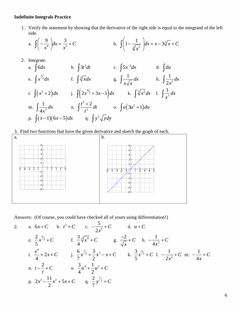
Indefinite Integrals Practice

1. Verify the statement by showing that the derivative of the right side is equal to the integrand of the left

side.

a. 4 3

9 3dx C

x x

b. 3

23

11 3dx x x C

x

2. Integrate.

a. 6dx b. 23t dt c.

35x dx

d. du

e. 3

2x dx f. 3 xdx g. 1

dxx x h.

3

1

2dx

x

i. 3 2x dx j. 4

32 3 1x x dx k. 23 x dx l.

3

1dx

x

m. 2

1

4dx

x n.

2

2

2tdt

t

o. 23 1u u du

p. 1 6 5x x dx q. 2y ydy

3. Find two functions that have the given derivative and sketch the graph of each.

a.

b.

Answers: (Of course, you could have checked all of yours using differentiation!)

2. a. 6x C b. 3t C c.

2

5

2C

x d. u C

e. 5

22

5x C f.

433

4x C g.

2C

x

h.

2

1

4C

x

i.

4

24

xx C j.

723

6 3

7 2x x x C k.

53

3

5x C l.

2

1

2C

x m.

1

4C

x

n. 2

t Ct

o. 4 23 1

4 2u u C

p. 3 211

2 52

x x x C q. 7

22

7y C

7

7.2 The Initial Value Problem

Learning Objectives

Find general solutions of differential equations

Use initial conditions to find particular solutions of differential equations

Introduction

In the Lesson on Indefinite Integrals Calculus we discussed how finding antiderivatives can be thought of as finding

solutions to differential equations: We now look to extend this discussion by looking at how we can

designate and find particular solutions to differential equations.

Let’s recall that a general differential equation will have an infinite number of solutions. We will look at one such equation

and see how we can impose conditions that will specify exactly one particular solution.

Example 1:

Suppose we wish to solve the following equation:

Solution:

We can solve the equation by integration and we have

We note that there are an infinite number of solutions. In some applications, we would like to designate exactly one

solution. In order to do so, we need to impose a condition on the function We can do this by specifying the value of

for a particular value of In this problem, suppose that add the condition that This will specify exactly one

value of and thus one particular solution of the original equation:

Substituting into our general solution gives or

Hence the solution is the particular solution of the original equation

satisfying the initial condition

We now can think of other problems that can be stated as differential equations with initial conditions. Consider the following example.

Example 2:

Suppose the graph of includes the point and that the slope of the tangent line to at any point is given by the

expression Find

Solution:

We can re-state the problem in terms of a differential equation that satisfies an initial condition.

8

with .

By integrating the right side of the differential equation we have

Hence is the particular solution of the original equation satisfying the initial

condition

Finally, since we are interested in the value , we put into our expression for and obtain:

Lesson Summary

1. We found general solutions of differential equations.

2. We used initial conditions to find particular solutions of differential equations.

Multimedia Link

The following applet allows you to set the initial equation for and then the slope field for that equation is displayed.

In magenta you'll see one possible solution for . If you move the magenta point to the initial value, then you will see

the graph of the solution to the initial value problem. Follow the directions on the page with the applet to explore this idea, and then try redoing the examples from this section on the applet. Slope Fields Applet.

Review Questions

In problems #1–3, solve the differential equation for

1.

2.

3.

In problems #4–7, solve the differential equation for given the initial condition.

4. and .

5. and

6. and

7. and 13 2

( ) 3f

8. Suppose the graph of f includes the point (-2, 4) and that the slope of the tangent line to f at x is -2x+4. Find

f(5).

9

In problems #9–10, find the function that satisfies the given conditions.

9. with and

10. with (4) 7f and (4) 25f

Review Answers

1.

2.

3.

4.

5.

6.

7.

8. ;

9.

10.

10

Initial Condition & Integration of Trig Functions Practice

1. Find the particular solution ( )y f x that satisfies the differential equation and initial condition.

a. '( ) 3 3, (1) 4f x x f b. '( ) 6 ( 1), (10) 10f x x x f

c. 3

2 3'( ) , 0, (2)

4

xf x x f

x

d.

2'( ) sec , 2 33

f x x f

2. Find the equation of the function f whose graph passes through the point.

'( ) 6 10, 4,2f x x

3. Find the function f that satisfies the given conditions.

a. "( ) 2, '(2) 5, (2) 10f x f f b. 2 3"( ) , '(8) 6, (0) 0f x x f f

4. Integrate.

a. (2sin 3cos )x x dx b. 1 csc cott t dt

c. 2csc cos d d. 2 sint t dt

Answers:

1. a. 3

2( ) 2 3 1f x x x b. 3 2( ) 2 3 1710f x x x

c. 2

1 1 1( )

2f x

x x

d. ( ) tan 3f x x

2. 3

2( ) 4 10 10f x x x

3. a. 2( ) 4f x x x b.

43

9( )

4f x x

4. a. 2cos 3sinx x C b. csct t C

c. cot sin C d.

3

cos3

tt C

11

7.3 The Area Problem

Learning Objectives

Use sigma notation to evaluate sums of rectangular areas

Find limits of upper and lower sums

Use the limit definition of area to solve problems

Introduction

In The Lesson The Calculus we introduced the area problem that we consider in integral calculus. The basic problem was this:

Suppose we are interested in finding the area between the axis and the curve of from

to

We approximated the area by constructing four rectangles, with the height of each rectangle equal to the maximum value of the function in the sub-interval.

We then summed the areas of the rectangles as follows:

and

We call this the upper sum since it is based on taking the maximum value of the function within each sub-interval. We noted that as we used more rectangles, our area approximation became more accurate.

We would like to formalize this approach for both upper and lower sums. First we note that the lower sums of the area

of the rectangles results in Our intuition tells us that the true area lies

12

somewhere between these two sums, or and that we will get closer to it by using more and more

rectangles in our approximation scheme.

In order to formalize the use of sums to compute areas, we will need some additional notation and terminology.

Sigma Notation

In The Lesson The Calculus we used a notation to indicate the upper sum when we increased our rectangles to

and found that our approximation . The notation we used to enabled us to indicate the sum

without the need to write out all of the individual terms. We will make use of this notation as we develop more formal definitions of the area under the curve.

Let’s be more precise with the notation. For example, the quantity was found by summing the areas of rectangles. We want to indicate this process, and we can do so by providing indices to the symbols used as

follows:

The sigma symbol with these indices tells us how the rectangles are labeled and how many terms are in the sum.

Useful Summation Formulas

We can use the notation to indicate useful formulas that we will have occasion to use. For example, you may recall that

the sum of the first integers is We can indicate this formula using sigma notation. The formula is given

here along with two other formulas that will become useful to us.

We can show from associative, commutative, and distributive laws for real numbers that

and

Example 1:

Compute the following quantity using the summation formulas:

Solution:

13

Another Look at Upper and Lower Sums

We are now ready to formalize our initial ideas about upper and lower sums.

Let be a bounded function in a closed interval and the partition of into subintervals.

We can then define the lower and upper sums, respectively, over partition , by

where is the minimum value of in the interval of length and is the maximum value of in the interval

of length

The following example shows how we can use these to find the area.

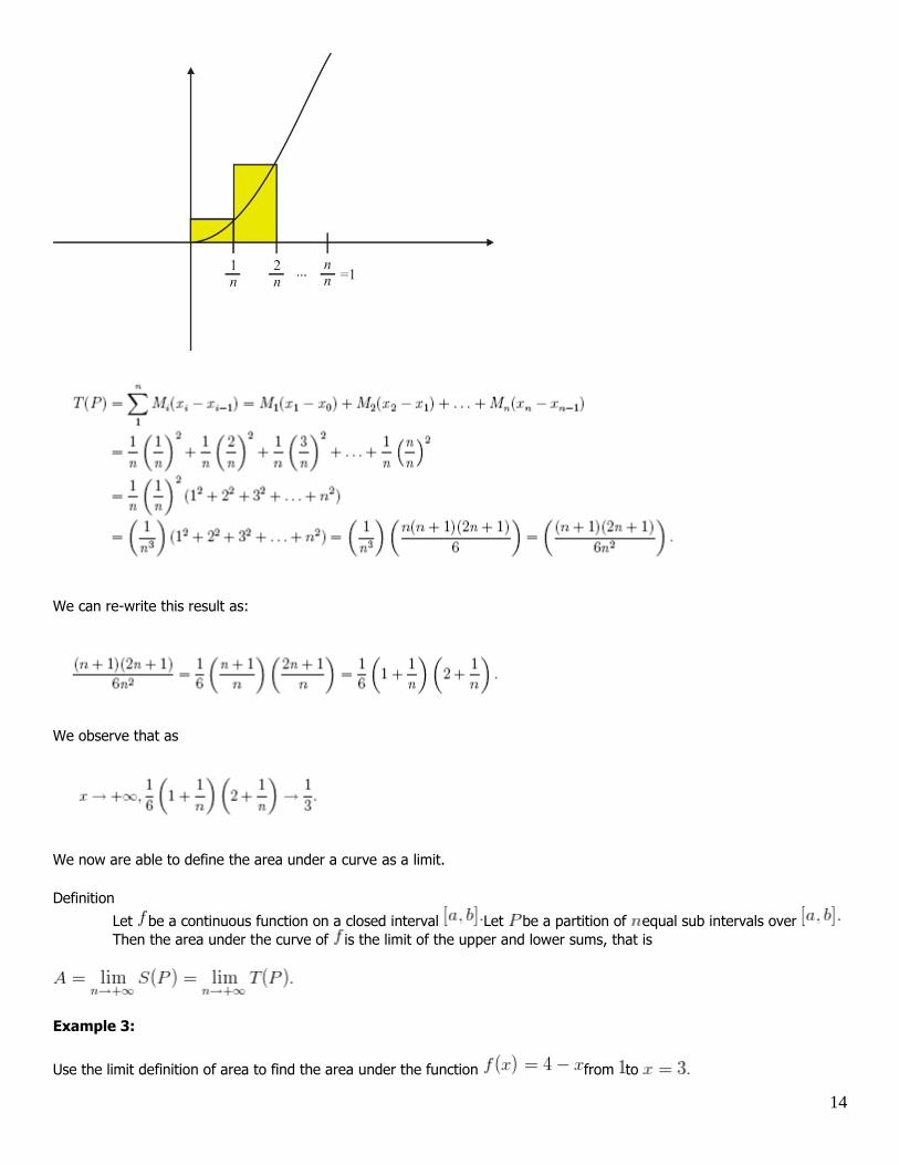
Example 2:

Show that the upper and lower sums for the function from to approach the value

Solution:

Let be a partition of equal sub intervals over We will show the result for the upper sums. By our definition we

have

We note that each rectangle will have width indicated:

14

We can re-write this result as:

We observe that as

We now are able to define the area under a curve as a limit.

Definition

Let be a continuous function on a closed interval Let be a partition of equal sub intervals over

Then the area under the curve of is the limit of the upper and lower sums, that is

Example 3:

Use the limit definition of area to find the area under the function from to

15

Solution:

If we partition the interval into equal sub-intervals, then each sub-interval will have length and height

as varies from to So we have and

Since , we then have by substitution

as . Hence the area is

This example may also be solved with simple geometry. It is left to the reader to confirm that the two methods yield the same area.

Lesson Summary

1. We used sigma notation to evaluate sums of rectangular areas.

2. We found limits of upper and lower sums. 3. We used the limit definition of area to solve problems.

Review Questions

In problems #1–2 , find the summations.

1.

2.

In problems #3–5, find and under the partition P.

3.

4.

5.

In problems #6–8, find the area under the curve using the limit definition of area.

16

6. from to

7. from to

8. from to

In problems #9–10, state whether the function is integrable in the given interval. Give a reason for your answer.

9. on the interval

10. on the interval

Review Answers

1.

2.

3. ;

(note that we have included areas under the x-axis as negative values.)

4. ;

5. ;

6.

7.

8.

9. Yes, since is continuous on

10. No, since ;

7.4 Definite Integrals

Learning Objectives

Use Riemann Sums to approximate areas under curves

Evaluate definite integrals as limits of Riemann Sums

Introduction

In the Lesson The Area Problem we defined the area under a curve in terms of a limit of sums.

where

17

and were examples of Riemann Sums. In general, Riemann Sums are of form where each

is the value we use to find the length of the rectangle in the sub-interval. For example, we used the maximum function value in each sub-interval to find the upper sums and the minimum function in each sub-interval to find the

lower sums. But since the function is continuous, we could have used any points within the sub-intervals to find the limit.

Hence we can define the most general situation as follows:

Definition

If is continuous on we divide the interval into sub-intervals of equal width with . We

let be the endpoints of these sub-intervals and let be any sample

points in these sub-intervals. Then the definite integral of from to is

Example 1:

Evaluate the Riemann Sum for from to using sub-intervals and taking the sample points to

be the midpoints of the sub-intervals.

Solution:

If we partition the interval into equal sub-intervals, then each sub-interval will have length So we

have and

18

Now let’s compute the definite integral using our definition and also some of our summation formulas.

Example 2:

Use the definition of the definite integral to evaluate

Solution:

Applying our definition, we need to find

We will use right endpoints to compute the integral. We first need to divide into sub-intervals of length

Since we are using right endpoints,

So

Recall that By substitution, we have

Hence

Before we look to try some problems, let’s make a couple of observations. First, we will soon not need to rely on the

summation formula and Riemann Sums for actual computation of definite integrals. We will develop several computational strategies in order to solve a variety of problems that come up. Second, the idea of definite integrals as approximating

the area under a curve can be a bit confusing since we may sometimes get results that do not make sense when

interpreted as areas. For example, if we were to compute the definite integral then due to the symmetry of

about the origin, we would find that This is because for every sample point we also have

is also a sample point with Hence, it is more accurate to say that gives us the net area between and If we wanted the total area bounded by the graph and the axis, then we would

compute .

19

Lesson Summary

1. We used Riemann Sums to approximate areas under curves.

2. We evaluated definite integrals as limits of Riemann Sums.

Multimedia Link

For video presentations on calculating definite integrals using Riemann Sums (13.0), see Riemann Sums, Part 1

(6:15) and Riemann Sums, Part 2 (8:32) .

The following applet lets you explore Riemann Sums of any function. You can change the bounds and the number of

partitions. Follow the examples given on the page, and then use the applet to explore on your own. Riemann Sums

Applet. Note: On this page the author uses Left- and Right- hand sums. These are similar to the sums and

that you have learned, particularly in the case of an increasing (or decreasing) function. Left-hand and Right-hand sums are frequently used in calculations of numerical integrals because it is easy to find the left and right endpoints of each

interval, and much more difficult to find the max/min of the function on each interval. The difference is not always

important from a numerical approximation standpoint; as you increase the number of partitions, you should see the Left-hand and Right-hand sums converging to the same value. Try this in the applet to see for yourself.

Review Questions

In problems #1–7 , use Riemann Sums to approximate the areas under the curves.

1. Consider from to Use Riemann Sums with four subintervals of equal lengths.

Choose the midpoints of each subinterval as the sample points.

2. Repeat problem #1 using geometry to calculate the exact area of the region under the graph of

from to (Hint: Sketch a graph of the region and see if you can compute its area using area

measurement formulas from geometry.) 3. Repeat problem #1 using the definition of the definite integral to calculate the exact area of the region under the

graph of from to

4. from to Use Riemann Sums with five subintervals of equal lengths. Choose the left endpoint of each subinterval as the sample points, or use trapezoids.

5. Repeat problem #4 using the definition of the definite integral to calculate the exact area of the region under the

graph of from to

6. Consider Compute the Riemann Sum of f on [0, 1] under each of the following situations. In each

case, use the right endpoint as the sample points, or use trapezoids. a. Two sub-intervals of equal length.

b. Five sub-intervals of equal length.

c. Ten sub-intervals of equal length. d. Based on your answers above, try to guess the exact area under the graph of f on [0, 1].

7. Consider . Compute the Riemann Sum of f on [0, 1] under each of the following situations. In each case, use the right endpoint as the sample points.

a. Two sub-intervals of equal length.

b. Five sub-intervals of equal length.

20

c. Ten sub-intervals of equal length.

d. Based on your answers above, try to guess the exact area under the graph of f on [0, 1].

8. Find the net area under the graph of ; to (Hint: Sketch the graph and check

for symmetry.)

9. Find the total area bounded by the graph of and the x-axis, from to

10. Use your knowledge of geometry to evaluate the following definite integral: (Hint: set

29y x and square both sides to see if you can recognize the region from geometry.)

Review Answers

1. 2. 3. 4. using the Left sum, Area = 13.68 using the Trapezoid Sum

5. 6.

a. using the Right sum, Area = 1.125 using the Trapezoid Sum

b. using the Right sum, Area = 1.02 using the Trapezoid Sum

c. using the Right sum, Area = 1.005 using the Trapezoid Sum

d. is a good guess

7. a. b. c. d.

8. The graph is symmetric about the origin; hence net Area = 0

9. Area = 1/2

10. The graph is that of a quarter circle of radius 3; hence Area = 9

4

7.5 Evaluating Definite Integrals

Learning Objectives

Use antiderivatives to evaluate definite integrals

Use the Mean Value Theorem for integrals to solve problems

Use general rules of integrals to solve problems

Introduction

In the Lesson on Definite Integrals, we evaluated definite integrals using the limit definition. This process was long and

tedious. In this lesson we will learn some practical ways to evaluate definite integrals. We begin with a theorem that provides an easier method for evaluating definite integrals. Newton discovered this method that uses antiderivatives to

calculate definite integrals.

Theorem:

If is continuous on the closed interval then

where is any antiderivative of

21

We sometimes use the following shorthand notation to indicate

The proof of this theorem is included at the end of this lesson. Theorem 4.1 is usually stated as a part of the Fundamental Theorem of Calculus, a theorem that we will present in the Lesson on the Fundamental Theorem of

Calculus. For now, the result provides a useful and efficient way to compute definite integrals. We need only find an antiderivative of the given function in order to compute its integral over the closed interval. It also gives us a result with

which we can now state and prove a version of the Mean Value Theorem for integrals. But first let’s look at a couple of examples.

Example 1:

Compute the following definite integral:

Solution:

Using the limit definition we found that We now can verify this using the theorem as follows:

We first note that is an antiderivative of Hence we have

We conclude the lesson by stating the rules for definite integrals, most of which parallel the rules we stated for the general indefinite integrals.

Given these rules together with Theorem 4.1, we will be able to solve a great variety of definite integrals.

Example 2:

Compute

22

Solution:

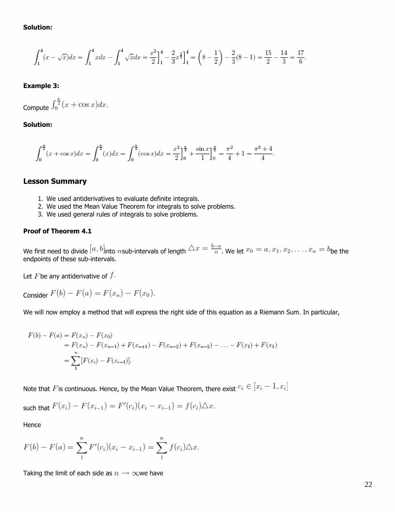
Example 3:

Compute

Solution:

Lesson Summary

1. We used antiderivatives to evaluate definite integrals. 2. We used the Mean Value Theorem for integrals to solve problems.

3. We used general rules of integrals to solve problems.

Proof of Theorem 4.1

We first need to divide into sub-intervals of length . We let be the endpoints of these sub-intervals.

Let be any antiderivative of

Consider

We will now employ a method that will express the right side of this equation as a Riemann Sum. In particular,

Note that is continuous. Hence, by the Mean Value Theorem, there exist

such that

Hence

Taking the limit of each side as we have

23

We note that the left side is a constant and the right side is our definition for .

Hence

Proof of Theorem 4.2

Let

By the Mean Value Theorem for derivatives, there exists such that

From Theorem 4.1 we have that is an antiderivative of Hence, and in particular,

Hence, by substitution we have

Note that Hence we have

and by our definition of we have

This theorem allows us to find for positive functions a rectangle that has base and height such that the area of

the rectangle is the same as the area given by In other words, is the average function value over

Review Questions

In problems #1–8, use antiderivatives to compute the definite integral.

1.

2.

3.

4.

5.

6.

7.

8. Find the average value of over [1, 9].

9. If f is continuous and show that f takes on the value 3 at least once on the interval [1, 4].

24

10. Your friend states that there is no area under the curve of on since he computed

Is he correct? Explain your answer.

Review Answers

1.

2. 1

6

3. = 2

2 52

4.

5.

6.

7.

8. 9. Apply the Mean Value Theorem for integrals.

10. He is partially correct. The definite integral computes the net area under the curve. However, the

area between the curve and the x-axis is given by: 0

0

2 sin 2 cos 4A xdx x

25

Practice with the Mean Value Theorem, Average Value & Properties of Integrals

Find the average value of the function over the interval. Then find all x-values in the interval for which the

function is equal to its average value.

1. 2( ) 6 , 2,2f x x 2. 2( ) 4 , 0,2f x x x

3. A deposit of $2250 is made in a savings account with an annual interest rate of 12%, compounded

continuously. Find the average balance in the account during the first 5 years.

4. In the United States, the annual death rate R (in deaths per 1000 people x years old) can be modeled by 2.036 2.8 58.14, 40 60R x x x . Find the average death rate for people between a) 40 and 50 years of

age, and b) 50 and 60 years of age.

5. Use the value 2

2

0

8

3x dx to evaluate the definite integral.

a. 0

2

2x dx

b. 2

2

2x dx

c. 2

2

0x dx

6. Use the value 2

3

04x dx to evaluate the definite integral.

a. 0

3

2x dx

b. 2

3

2x dx

c. 2

3

03x dx

7. Use the values 5

0( ) 8f x dx and

5

0( ) 3g x dx to evaluate the definite integral.

a. 5

0( ) ( )f x g x dx b.

5

0( ) ( )f x g x dx c.

5

0( ) ( )f x f x dx

d. 5

04 ( )f x dx e.

5

0( ) 3 ( )f x g x dx f.

5

5( )f x dx g.

0

5( )f x dx

Answers:

1. average value = 14

3 2. average value =

4

3

2 31.155

3x

2 52 1.868

3

2 52 .714

3

x

x

3. $3082.95

4. a) 5.34 deaths per 1000 people b) 13.34 deaths per 1000 people

5. a. 8

3 b.

16

3 c.

8

3

6. a. 4 b. 0 c. 12

7. a. 11 b. 5 c. 0

d. -32 e. -1 f. 0 g. -8

26

Integral Properties & Average Value HW

Use the given info and the properties of integrals to evaluate the requested definite integrals.

1.) Given:

2

0

8( )

3f x dx , and ( )f x is an even function

a.)

0

2

( )f x dx

b.)

2

2

( )f x dx

c.)

2

0

5 ( )f x dx

2.) Given:

2

0

( ) 4g x dx , and ( )f x is an odd function

a.)

0

2

( )g x dx

b.)

2

2

( )g x dx

c.)

2

0

5 ( )g x dx

3.) Given:

5

0

( ) 8f x dx and

5

0

( ) 3g x dx

a.) 5

0( ) ( )f x g x dx b.)

5

0( ) ( )f x g x dx c.)

5

0( ) ( )f x f x dx

d.) 5

0( ) 3 ( )f x g x dx e.)

5

5( )f x dx f.)

0

5( )f x dx

g.) 5

0( ) ( )f x g x dx h.)

5

0

( )

( )

f xdx

g x

Find the average value of the function over the given interval, and find the x-value in the interval where the

function takes on the average value.

4.) 2( ) 6 , [ 2, 2]f x x

5.) 2( ) 4 , [0, 2]f x x x

Answers:

1.) 8/3, 16/3, 40/3

2.) –4, 0, 20

3.) 11, 5, 0, –1, 0, –8, g & h cannot be done with the

given info – multiplying / dividing areas does not yield

areas!

4.) AV = 14/3, 1.155 [ 2,2]x

5.) AV = 4/3, .714,1.868 [0,2]x

27

7.6 The Fundamental Theorem of Calculus

Learning Objectives

Use the Fundamental Theorem of Calculus to evaluate definite integrals

Introduction

In the Lesson on Evaluating Definite Integrals, we evaluated definite integrals using antiderivatives. This process was much more efficient than using the limit definition. In this lesson we will state the Fundamental Theorem of Calculus and

continue to work on methods for computing definite integrals.

Fundamental Theorem of Calculus:

Let be continuous on the closed interval

1. If function is defined by on , then on

2. If is any antiderivative of on then

We first note that we have already proven part 2 as Theorem 4.1. The proof of part 1 appears at the end of this lesson.

Think about this Theorem. Two of the major unsolved problems in science and mathematics turned out to be solved by calculus which was invented in the seventeenth century. These are the ancient problems:

1. Find the areas defined by curves, such as circles or parabolas. 2. Determine an instantaneous rate of change or the slope of a curve at a point.

With the discovery of calculus, science and mathematics took huge leaps, and we can trace the advances of the space

age directly to this Theorem.

Let’s continue to develop our strategies for computing definite integrals. We will illustrate how to solve the problem of

finding the area bounded by two or more curves.

Example 1:

Find the area between the curves of and

Solution:

We first observe that there are no limits of integration explicitly stated here. Hence we need to find the limits by analyzing

the graph of the functions.

28

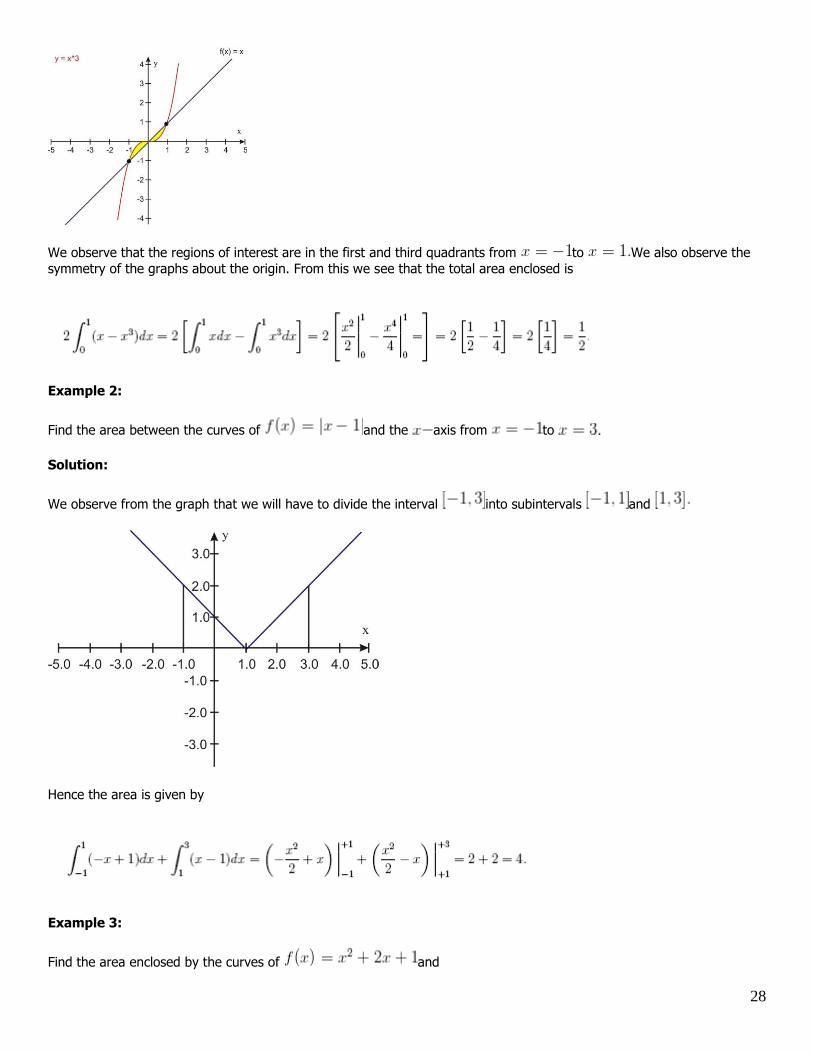
We observe that the regions of interest are in the first and third quadrants from to We also observe the

symmetry of the graphs about the origin. From this we see that the total area enclosed is

Example 2:

Find the area between the curves of and the axis from to

Solution:

We observe from the graph that we will have to divide the interval into subintervals and

Hence the area is given by

Example 3:

Find the area enclosed by the curves of and

29

Solution:

The graph indicates the area we need to focus on.

Before providing another example, let’s look back at the first part of the Fundamental Theorem. If function is defined

by on then on Observe that if we differentiate the integral with respect to we have

This fact enables us to compute derivatives of integrals as in the following example.

Example 4:

Use the Fundamental Theorem to find the derivative of the following function:

Solution:

While we could easily integrate the right side and then differentiate, the Fundamental Theorem enables us to find the

answer very routinely.

30

This application of the Fundamental Theorem becomes more important as we encounter functions that may be more

difficult to integrate such as the following example.

Example 5:

Use the Fundamental Theorem to find the derivative of the following function:

Solution:

In this example, the integral is more difficult to evaluate. The Fundamental Theorem enables us to find the answer routinely.

Lesson Summary

1. We used the Fundamental Theorem of Calculus to evaluate definite integrals.

Fundamental Theorem of Calculus

Let be continuous on the closed interval

1. If function is defined by , on then on

2. If is any antiderivative of on then

We first note that we have already proven part 2 as Theorem 4.1.

Proof of Part 1.

1. Consider on

2.

Then by our rules for definite integrals.

3. Then . Hence

4. Since is continuous on and then we can select such that is the minimum

value of and is the maximum value of in Then we can consider as a lower sum and

as an upper sum of from to Hence

5.

31

6. By substitution, we have:

7. By division, we have

8. When is close to then both and are close to by the continuity of

9. Hence Similarly, if then Hence,

10. By the definition of the derivative, we have that

for every Thus, is an antiderivative of on

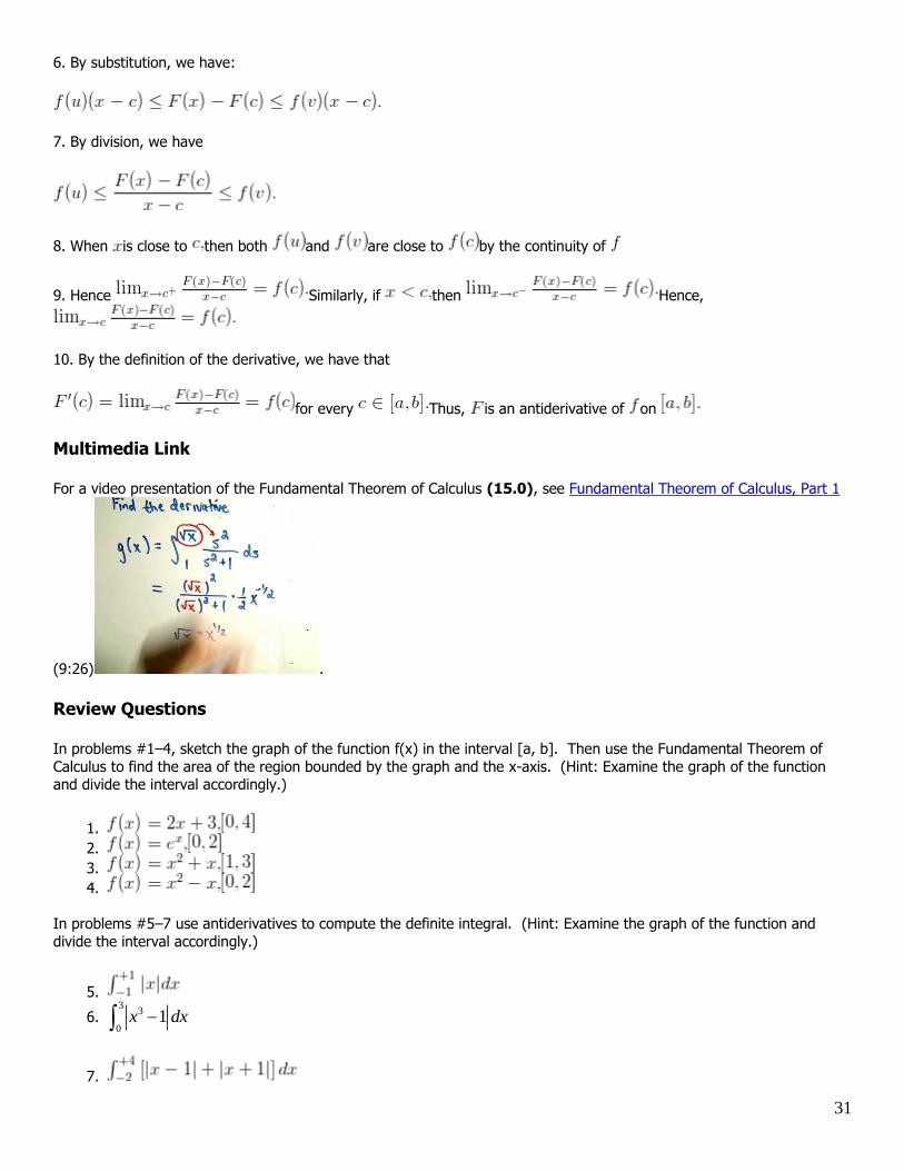
Multimedia Link

For a video presentation of the Fundamental Theorem of Calculus (15.0), see Fundamental Theorem of Calculus, Part 1

(9:26) .

Review Questions

In problems #1–4, sketch the graph of the function f(x) in the interval [a, b]. Then use the Fundamental Theorem of

Calculus to find the area of the region bounded by the graph and the x-axis. (Hint: Examine the graph of the function and divide the interval accordingly.)

1.

2.

3.

4.

In problems #5–7 use antiderivatives to compute the definite integral. (Hint: Examine the graph of the function and

divide the interval accordingly.)

5.

6. 3

3

01x dx

7.

32

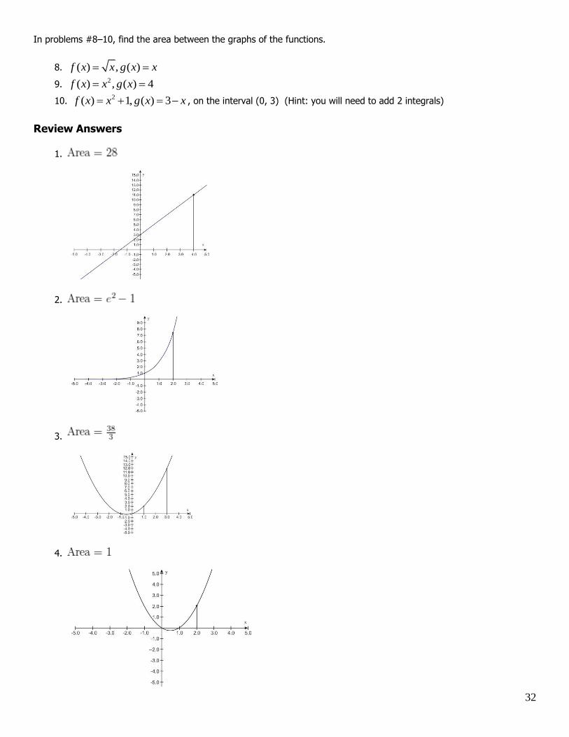
In problems #8–10, find the area between the graphs of the functions.

8. ( ) , ( )f x x g x x

9. 2( ) , ( ) 4f x x g x

10. 2( ) 1, ( ) 3f x x g x x , on the interval (0, 3) (Hint: you will need to add 2 integrals)

Review Answers

1.

2.

3.

4.

33

5. 6. 18.75

7. 8. Area = 1/6

9. Area = 32/3

10. Area = 59

6

7.7 Integration by Substitution

Learning Objectives

Integrate composite functions

Use change of variables to evaluate definite integrals

Use substitution to compute definite integrals

Introduction

34

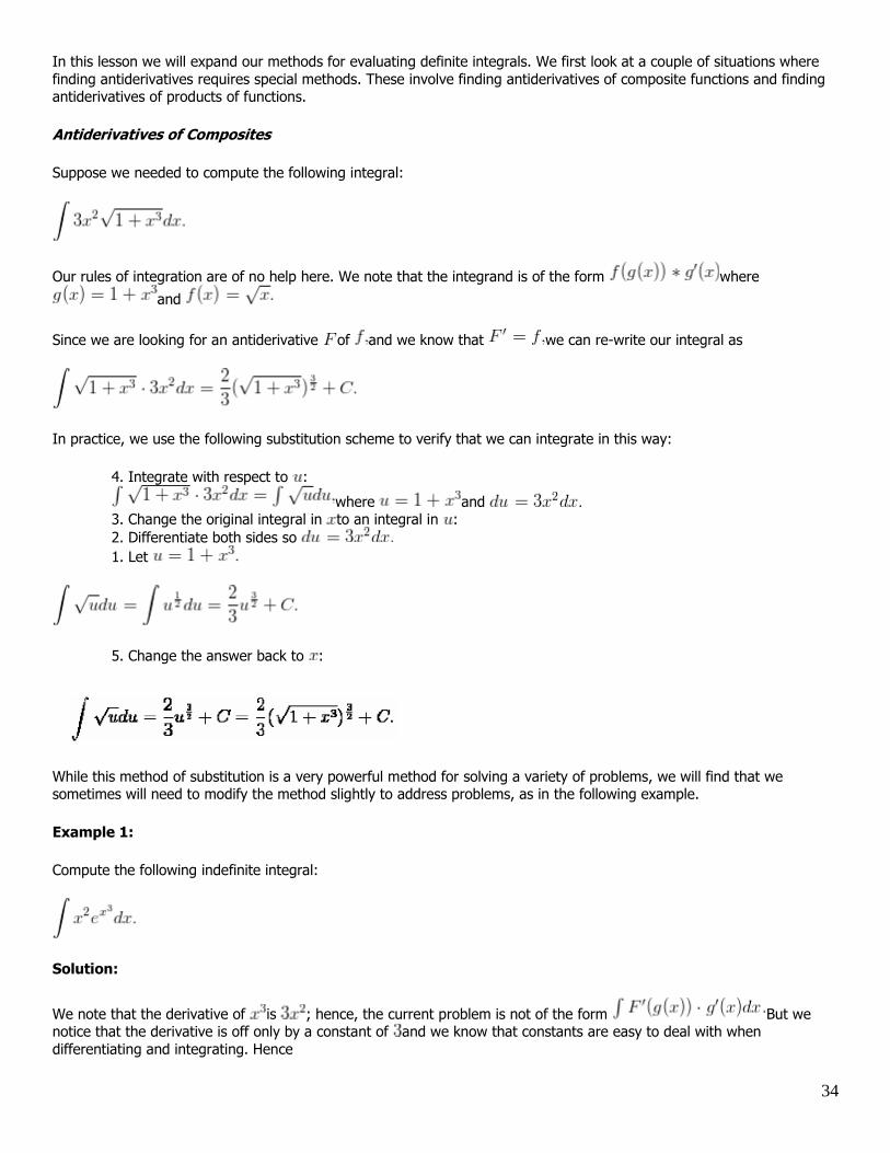
In this lesson we will expand our methods for evaluating definite integrals. We first look at a couple of situations where

finding antiderivatives requires special methods. These involve finding antiderivatives of composite functions and finding antiderivatives of products of functions.

Antiderivatives of Composites

Suppose we needed to compute the following integral:

Our rules of integration are of no help here. We note that the integrand is of the form where

and

Since we are looking for an antiderivative of and we know that we can re-write our integral as

In practice, we use the following substitution scheme to verify that we can integrate in this way:

4. Integrate with respect to :

where and 3. Change the original integral in to an integral in :

2. Differentiate both sides so

1. Let

5. Change the answer back to :

While this method of substitution is a very powerful method for solving a variety of problems, we will find that we sometimes will need to modify the method slightly to address problems, as in the following example.

Example 1:

Compute the following indefinite integral:

Solution:

We note that the derivative of is ; hence, the current problem is not of the form But we notice that the derivative is off only by a constant of and we know that constants are easy to deal with when

differentiating and integrating. Hence

35

Let

Then

Then and we are ready to change the original integral from to an integral in and integrate:

Changing back to , we have

We can also use this substitution method to evaluate definite integrals. If we attach limits of integration to our first example, we could have a problem such as

The method still works. However, we have a choice to make once we are ready to use the Fundamental Theorem to

evaluate the integral.

Recall that we found that for the indefinite integral. At this point, we could evaluate the integral by changing the answer back to or we could evaluate the integral in But we need to be careful. Since the

original limits of integration were in , we need to change the limits of integration for the equivalent integral in Hence,

where

Integrating Products of Functions

We are not able to state a rule for integrating products of functions, but we can get a relationship that is almost as effective. Recall how we differentiated a product of functions:

So by integrating both sides we get

or

In order to remember the formula, we usually write it as

36

We refer to this method as integration by parts. The following example illustrates its use.

Example 2:

Use integration by parts method to compute

Solution:

We note that our other substitution method is not applicable here. But our integration by parts method will enable us to reduce the integral down to one that we can easily evaluate.

Let and then and

By substitution, we have

We can easily evaluate the integral and have

And should we wish to evaluate definite integrals, we need only to apply the Fundamental Theorem to the antiderivative.

Lesson Summary

1. We integrated composite functions. 2. We used change of variables to evaluate definite integrals.

3. We used substitution to compute definite integrals.

Review Questions

Compute the integrals in problems #1–8.

1.

2.

3.

4.

5.

6.

7.

8.

37

Review Answers

1.

2.

3.

4.

5.

6.

7.

8.

38

Integration by Substitution Practice

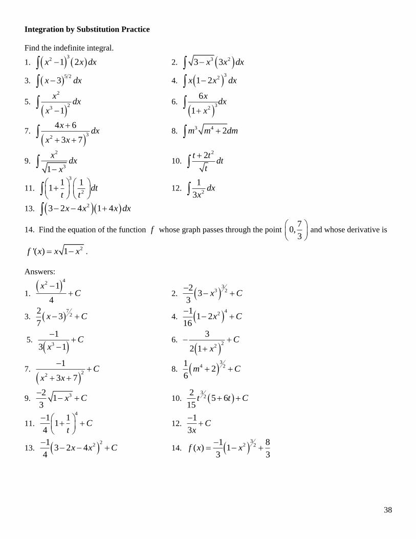
Find the indefinite integral.

1. 3

2 1 2x x dx 2. 3 23 3x x dx

3. 5 2

3x dx 4. 3

21 2x x dx

5.

2

23 1

xdx

x 6.

3

2

6

1

xdx

x

7.

3

2

4 6

3 7

xdx

x x

8.

3 4 2m m dm

9.

2

31

xdx

x 10.

22t tdt

t

11.

3

2

1 11 dt

t t

12.

2

1

3dx

x

13. 23 2 4 1 4x x x dx

14. Find the equation of the function f whose graph passes through the point 7

0,3

and whose derivative is

2'( ) 1f x x x .

Answers:

1.

42 1

4

xC

2.

33 22

33

x C

3. 7

22

37

x C 4. 4

211 2

16x C

5. 3

1

3 1C

x

6.

2

2

3

2 1C

x

7.

2

2

1

3 7C

x x

8.

34 21

26

m C

9. 32

13

x C

10. 3

22

5 615

t t C

11.

41 1

14

Ct

12.

1

3C

x

13. 2

213 2 4

4x x C

14.

32 21 8

( ) 13 3

f x x

39

General Power Rule HW 1

Integrate!

1.) 3

22 1x x dx

2.) 2 33 3x x dx

3.) 523x dx

4.) 3

21 2x x dx

5.)

2

23 1

xdx

x

6.)

3

2

4 6

3 7

xdx

x x

7.) Find the equation of the function ( )f x whose graph passes through the point 7

0,3

and whose derivative is

2( ) 1f x x x .

Answers:

1.)

42 1

4

xC

2.) 3232

33

x C

3.) 72

23

7x C

4.) 4

211 2

16x C

5.) 3

1

3 1C

x

6.)

2

2

1

3 7C

x x

7.) 3221 8

( ) 13 3

f x x

40

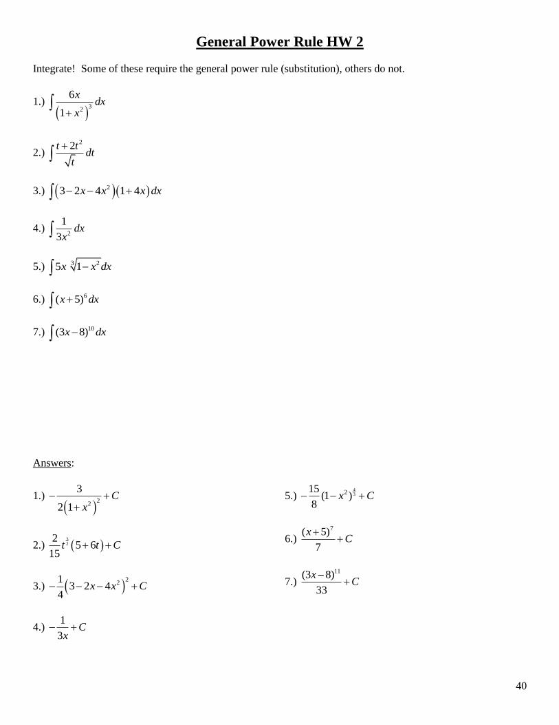
General Power Rule HW 2

Integrate! Some of these require the general power rule (substitution), others do not.

1.)

3

2

6

1

xdx

x

2.) 22t t

dtt

3.) 23 2 4 1 4x x x dx

4.) 2

1

3dx

x

5.) 3 25 1x x dx

6.) 6( 5)x dx

7.) 10(3 8)x dx

Answers:

1.)

2

2

3

2 1C

x

2.) 32

25 6

15t t C

3.) 2

213 2 4

4x x C

4.) 1

3C

x

5.) 43215

(1 )8

x C

6.) 7( 5)

7

xC

7.) 11(3 8)

33

xC

41

Practice with Integration by Substitution Involving Trig

Evaluate the integral.

1. cos6xdx 2. 2sinx x dx

3. 2csc

2

xdx 4. csc2 cot 2x xdx

5. 2cot cscx xdx 6.

2

sin

cos

xdx

x

7. sin x

dxx

Answers:

1. 1

sin 66

x C 2. 21

cos2

x C

3. 2cot2

xC 4.

1csc2

2x C

5. 3

22

cot3

x C

6. sec x C

7. 2cos x C

42

Trig Integrals HW

Integrate!

1.) cos6xdx

2.) 2sin( )x x dx

3.) 2csc2

xdx

4.) csc2 cot 2x xdx

5.) 2tan secx xdx

6.) 2

sin

cos

xdx

x

7.) sin x

dxx

Answers:

1.) sin 6

6

xC

2.) 2cos( )

2

xC

3.) 2cot2

xC

4.) csc2

2

xC

5.) 32

2tan

3x C

6.) sec x C

7.) 2cos x C

43

7.8 Numerical Integration

Learning Objectives

Use the Trapezoidal Rule to solve problems

Estimate errors for the Trapezoidal Rule

Use Simpson’s Rule to solve problems

Estimate Errors for Simpson’s Rule

Introduction

Recall that we used different ways to approximate the value of integrals. These included Riemann Sums using left and right endpoints, as well as midpoints for finding the length of each rectangular tile. In this lesson we will learn two other

methods for approximating integrals. The first of these, the Trapezoidal Rule, uses areas of trapezoidal tiles to

approximate the integral. The second method, Simpson’s Rule, uses parabolas to make the approximation.

Trapezoidal Rule

Let’s recall how we would use the midpoint rule with rectangles to approximate the area under the graph of

from to

If instead of using the midpoint value within each sub-interval to find the length of the corresponding rectangle, we could have instead formed trapezoids by joining the maximum and minimum values of the function within each sub-interval:

The area of a trapezoid is , where and are the lengths of the parallel sides and is the height. In our

trapezoids the height is and and are the values of the function. Therefore in finding the areas of the trapezoids

we actually average the left and right endpoints of each sub-interval. Therefore a typical trapezoid would have the area

44

To approximate with of these trapezoids, we have

Example 1:

Use the Trapezoidal Rule to approximate with .

Solution:

We find

Of course, this estimate is not nearly as accurate as we would like. For functions such as we can easily find

an antiderivative with which we can apply the Fundamental Theorem that But it is not always

easy to find an antiderivative. Indeed, for many integrals it is impossible to find an antiderivative. Another issue concerns the questions about the accuracy of the approximation. In particular, how large should we take n so that the Trapezoidal

Estimate for is accurate to within a given value, say ? As with our Linear Approximations in the Lesson on

Approximation Errors, we can state a method that ensures our approximation to be within a specified value.

Error Estimates for Simpson's Rule

We would like to have confidence in the approximations we make. Hence we can choose to ensure that the errors are within acceptable boundaries. The following method illustrates how we can choose a sufficiently large

Suppose for Then the error estimate is given by

Example 2:

Find so that the Trapezoidal Estimate for is accurate to

Solution:

45

We need to find such that We start by noting that for Hence we

can take to find our error bound.

We need to solve the following inequality for :

Hence we must take to achieve the desired accuracy.

From the last example, we see one of the weaknesses of the Trapezoidal Rule—it is not very accurate for functions where

straight line segments (and trapezoid tiles) do not lead to a good estimate of area. It is reasonable to think that other methods of approximating curves might be more applicable for some functions. Simpson’s Rule is a method that uses

parabolas to approximate the curve.

Simpson’s Rule:

As was true with the Trapezoidal Rule, we divide the interval into sub-intervals of length We then construct parabolas through each group of three consecutive points on the graph. The graph below shows this process for the first three such parabolas for the case of sub-intervals. You can see that every interval except the first and

last contains two estimates, one too high and one too low, so the resulting estimate will be more accurate.

Using parabolas in this way produces the following estimate of the area from Simpson’s Rule:

We note that it has a similar appearance to the Trapezoidal Rule. However, there is one distinction we need to note. The

process of using three consecutive to approximate parabolas will require that we assume that must always be an even number.

Error Estimates for the Trapezoidal Rule

As with the Trapezoidal Rule, we have a formula that suggests how we can choose to ensure that the errors are within acceptable boundaries. The following method illustrates how we can choose a sufficiently large

46

Suppose for Then the error estimate is given by

Example 3:

a. Use Simpson’s Rule to approximate with .

Solution:

We find

This turns out to be a pretty good estimate, since we know that

Therefore the error is less than .

b. Find so that the Simpson Rule Estimate for is accurate to

Solution:

We need to find such that We start by noting that for Hence we

can take to find our error bound:

Hence we need to solve the following inequality for :

We find that

47

Hence we must take to achieve the desired accuracy.

Technology Note: Estimating a Definite Integral with a TI-83/84 Calculator

We will estimate the value of .

1. Graph the function with the [WINDOW] setting shown below.

2. The graph is shown in the second screen. 3. Press 2nd [CALC] and choose option 7 (see menu below)

4. When the fourth screen appears, press [1] [ENTER] then [4] [ENTER] to enter the lower and upper limits. 5. The final screen gives the estimate, which is accurate to 7 decimal places.

Lesson Summary

1. We used the Trapezoidal Rule to solve problems. 2. We estimated errors for the Trapezoidal Rule.

3. We used Simpson’s Rule to solve problems.

4. We estimated Errors for Simpson’s Rule.

Multimedia Links

For video presentations of Simpson's Rule (21.0), see Simpson's Rule, Approximate Integration

(7:21)

48

and Math Video Tutorials by James Sousa, Simpson's Rule of Numerical Integration (8:48) .

For a video presentation of Newton's Method (21.0), see Newton's Method (7:29) .

Review Question

1. Use the Trapezoidal Rule to approximate with

2. Use the Trapezoidal Rule to approximate with

3. Use the Trapezoidal Rule to approximate with

4. Use the Trapezoidal Rule to approximate with

5. How large should you take n so that the Trapezoidal Estimate for is accurate to within .001?

6. Use Simpson’s Rule to approximate with

7. Use Simpson’s Rule to approximate with

8. Use Simpson’s Rule to approximate with

9. Use Simpson’s Rule to approximate with

10. How large should you take n so that the Simpson Estimate for is accurate to within .00001?

Review Answers

1.

2.

3.

4. 5. Take

6.

7.

8.

9. 10. Take

49

7.9 Area Between Two Curves

Learning Objectives

A student will be able to:

Compute the area between two curves with respect to the and axes.

In the last chapter, we introduced the definite integral to find the area between a curve and the axis over an interval

In this lesson, we will show how to calculate the area between two curves.

Consider the region bounded by the graphs and between and as shown in the figures below. If the two graphs lie above the axis, we can interpret the area that is sandwiched between them as the area under the graph of

subtracted from the area under the graph

Therefore, as the graphs show, it makes sense to say that

50

[Area under (Fig. 1a)] [Area under (Fig. 1b)] [Area between and (Fig. 1c)],

This relation is valid as long as the two functions are continuous and the upper function on the interval

The Area Between Two Curves (With respect to the axis)

If and are two continuous functions on the interval and for all values of in the interval, then the

area of the region that is bounded by the two functions is given by

Example 1:

Find the area of the region enclosed between and

Solution:

We first make a sketch of the region (Figure 2) and find the end points of the region. To do so, we simply equate the two

functions,

and then solve for

from which we get and

So the upper and lower boundaries intersect at points and

As you can see from the graph, and hence and in the interval Applying the area formula,

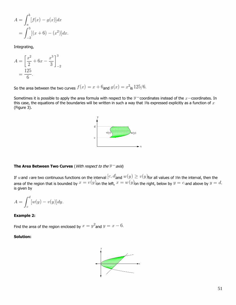
51

Integrating,

So the area between the two curves and is

Sometimes it is possible to apply the area formula with respect to the coordinates instead of the coordinates. In

this case, the equations of the boundaries will be written in such a way that is expressed explicitly as a function of (Figure 3).

The Area Between Two Curves (With respect to the axis)

If and are two continuous functions on the interval and for all values of in the interval, then the

area of the region that is bounded by on the left, on the right, below by and above by

is given by

Example 2:

Find the area of the region enclosed by and

Solution:

52

As you can see from Figure 4, the left boundary is and the right boundary is The region extends over

the interval However, we must express the equations in terms of We rewrite

Thus

Multimedia Links

For a video presentation of the area between two graphs (14.0)(16.0), see Math Video Tutorials by James Sousa, Area

Between Two Graphs (6:12) .

For an additional video presentation of the area between two curves (14.0)(16.0), see Just Math Tutoring, Finding

Areas Between Curves (9:50) .

53

Review Questions

In problems #1 - 7, sketch the region enclosed by the curves and find the area.

1. on the interval

2. on the interval

3. 4. [0, 2]

5. integrate with respect to y

6.

7.

8. Find the area enclosed by and

9. If the area enclosed by the two functions and is 2, what is the value of k?

10. Find the horizontal line y = k that divides the region between and into two equal areas.

Review Answers

1. 2. 3.

4.

5.

6.

7.

8. 9.

10. 3

9

4y

54

Area Between Two Curves Practice

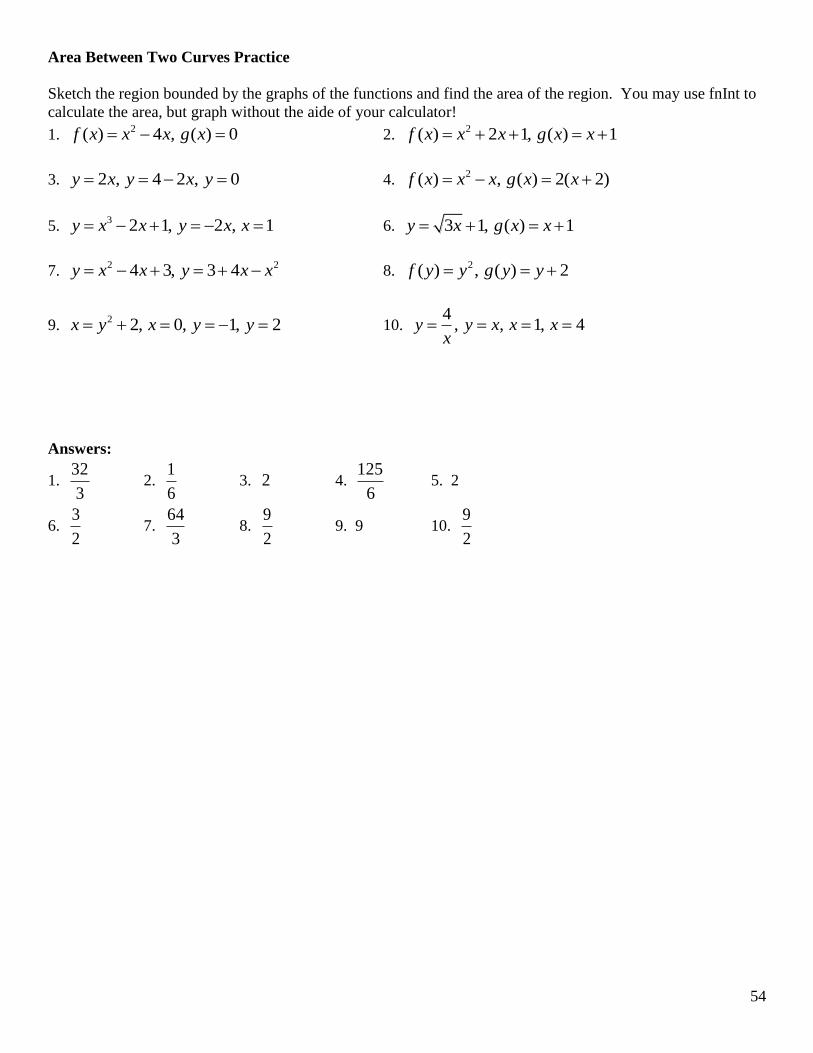
Sketch the region bounded by the graphs of the functions and find the area of the region. You may use fnInt to

calculate the area, but graph without the aide of your calculator!

1. 2( ) 4 , ( ) 0f x x x g x 2.

2( ) 2 1, ( ) 1f x x x g x x

3. 2 , 4 2 , 0y x y x y 4. 2( ) , ( ) 2( 2)f x x x g x x

5. 3 2 1, 2 , 1y x x y x x 6. 3 1, ( ) 1y x g x x

7. 2 24 3, 3 4y x x y x x 8.

2( ) , ( ) 2f y y g y y

9. 2 2, 0, 1, 2x y x y y 10.

4, , 1, 4y y x x x

x

Answers:

1. 32

3 2.

1

6 3. 2 4.

125

6 5. 2

6. 3

2 7.

64

3 8.

9

2 9. 9 10.

9

2

55

Area Between 2 Curves HW

Find the area between the curves.

1.) 2; 2x y x y

2.) 2 4 4;4 16y x x y

3.) 3;x y x y

4.) 2 ; 2 4y x x y x

5.) 3 2 1; 2 ; 1y x x y x x

Answers:

1.) 2

2

1

92

2y y dy

2.)

5 2

4

16 4 243

4 4 8

y ydy

3.)

0 1

3 3

1 0

1

2y y dy y y dy

4.) 4

2

1

1252 4

6x x x dx

5.) 1

3

1

2 1 2 2x x x dx