ORNL/TM-2012/176

INDDGO:Integrated Network Decomposition& Dynamic programming forGraph Optimization

October 2012Chris Groer1

Blair D. Sullivan1

Dinesh Weerapurage1

1This work was supported by the Department of Energy Office of Science, Office ofAdvanced Scientific Computing Research

DOCUMENT AVAILABILITY

Reports produced after January 1, 1996, are generally available free via theU.S. Department of Energy (DOE) Information Bridge:

Web Site: http://www.osti.gov/bridge

Reports produced before January 1, 1996, may be purchased by mem-bers of the public from the following source:

National Technical Information Service5285 Port Royal RoadSpringfield, VA 22161Telephone: 703-605-6000 (1-800-553-6847)TDD: 703-487-4639Fax: 703-605-6900E-mail: info@ntis.fedworld.govWeb site: http://www.ntis.gov/support/ordernowabout.htm

Reports are available to DOE employees, DOE contractors, EnergyTechnology Data Exchange (ETDE), and International Nuclear InformationSystem (INIS) representatives from the following sources:

Office of Scientific and Technical InformationP.O. Box 62Oak Ridge, TN 37831Telephone: 865-576-8401Fax: 865-576-5728E-mail: reports@adonis.osti.govWeb site: http://www.osti.gov/contact.html

This report was prepared as an account of work spon-sored by an agency of the United States Government.Neither the United States nor any agency thereof, norany of their employees, makes any warranty, express orimplied, or assumes any legal liability or responsibil-ity for the accuracy, completeness, or usefulness of anyinformation, apparatus, product, or process disclosed,or represents that its use would not infringe privatelyowned rights. Reference herein to any specific com-mercial product, process, or service by trade name,trademark, manufacturer, or otherwise, does not nec-essarily constitute or imply its endorsement, recom-mendation, or favoring by the United States Govern-ment or any agency thereof. The views and opinionsof authors expressed herein do not necessarily state orreflect those of the United States Government or anyagency thereof.

ORNL-2012/176

INDDGO: Integrated Network Decomposition & Dynamicprogramming for Graph Optimization

Chris GroerBlair D. Sullivan

Dinesh Weerapurage

Date Published: October 2012

Prepared byOAK RIDGE NATIONAL LABORATORY

P. O. Box 2008Oak Ridge, Tennessee 37831-6285

managed byUT-Battelle, LLC

for theU. S. DEPARTMENT OF ENERGYunder contract DE-AC05-00OR22725

Contents

List of Figures v

Abstract vii

1 Introduction 1

2 Constructing Tree Decompositions 12.1 Elimination Ordering Heuristics . . . . . . . . . . . . . . . . . 4

3 Solving Maximum Weighted Independent Set 63.1 Implementation Details . . . . . . . . . . . . . . . . . . . . . 7

3.1.1 Set operations . . . . . . . . . . . . . . . . . . . . . . 73.1.2 Finding all independent sets . . . . . . . . . . . . . . . 83.1.3 Memory-efficient storage . . . . . . . . . . . . . . . . . 83.1.4 Dynamic programming implementation . . . . . . . . 10

3.2 Memory Usage . . . . . . . . . . . . . . . . . . . . . . . . . . 103.2.1 Refining the tree decomposition . . . . . . . . . . . . . 113.2.2 Memory usage estimation . . . . . . . . . . . . . . . . 13

4 Computational Results 144.1 Partial k-trees . . . . . . . . . . . . . . . . . . . . . . . . . . . 144.2 Comparison with other algorithms . . . . . . . . . . . . . . . 154.3 Results on large width graphs . . . . . . . . . . . . . . . . . . 174.4 Estimating the Memory Usage . . . . . . . . . . . . . . . . . 19

5 Obtaining and Running the Code 195.1 Algorithm options . . . . . . . . . . . . . . . . . . . . . . . . 205.2 Example Usage . . . . . . . . . . . . . . . . . . . . . . . . . . 20

6 Conclusion 20

7 Acknowledgments 22

iii

List of Figures

1 A comparison of the average width and average running timeof various heuristics on a large set of benchmark problems . . 6

2 The maximum independent set in the graph is {A,D,F,H},and A is the only vertex in this set also in the root node.Therefore, B and C can be removed from the tree decompo-sition in the refinement procedure. . . . . . . . . . . . . . . . 13

3 The running time and memory usage of the other methodsremain roughly constant as the width varies while n and mremain constant. The tree decomposition based approach re-quires more memory as the width increases. . . . . . . . . . . 15

4 The memory usage and running time of our dynamic pro-gramming algorithm on large-width graphs. . . . . . . . . . . 18

5 The figure on the left shows a diagram of a width 35 decom-position where tree nodes are red if their bag has 36 vertices,blue if 35 vertices, and gradations of purple for smaller bagsizes. The diagram on the right shows the same decompo-sition after it is transformed into a nice decomposition withthe make nice option. . . . . . . . . . . . . . . . . . . . . . . 22

v

Abstract

It is well-known that dynamic programming algorithms can utilize tree de-compositions to provide a way to solve some NP -hard graph optimizationproblems where the complexity is polynomial in the number of nodes andedges in the graph, but exponential in the width of the underlying tree de-composition. However, there has been relatively little computational workdone to determine the practical utility of such dynamic programming al-gorithms. We have developed software to construct tree decompositionsusing various heuristics and have created a fast, memory-efficient dynamicprogramming implementation for solving maximum weighted independentset. We describe our software and the algorithms we have implemented,focusing on memory saving techniques for the dynamic programming. Wecompare the running time and memory usage of our implementation withother techniques for solving maximum weighted independent set, includinga commercial integer programming solver and a semi-definite programmingsolver. Our results indicate that it is possible to solve some instances wherethe underlying decomposition has width much larger than suggested by theliterature. For certain types of problems, our dynamic programming coderuns several times faster than these other methods.

vii

1. Introduction

Tree decompositions were introduced by Robertson and Seymour in 1984 inone of their papers on structural graph theory [22]. These decompositionsprovide a combinatorial metric for the “distance” from a graph to a tree,known as the width of a decomposition. The minimal achievable width fora graph is its treewidth, and can be thought of as a measure of how “tree-like” a graph is. Although tree decompositions were introduced as toolsfor proving the Graph Minors Theorem [21], these mappings have gainedimportance in computational graph theory, as they allow numerous NP -hardgraph problems to be solved in polynomial time for graphs with boundedtreewidth [11]. We begin by giving some necessary definitions, then proceedto describe how to compute and use these decompositions in algorithms.

Formally, a tree decomposition of a graph G = (V,E) is a pair (X,T ),where X = {X1, . . . , Xn} is a collection of subsets of V , and T = (I, F ) is atree with I = {1, . . . , n}, satisfying three conditions:

1. the union of the subsets Xi is equal to the vertex set V (1 ≤ i ≤ n),

2. for every edge uv in G, {u, v} ⊆ Xi for some i ∈ {1, 2, . . . , n}, and

3. for every v ∈ V , if Xi and Xj contain v for some i, j ∈ {1, 2, . . . , n},then Xk also contains v for all k on the (unique) path in T connectingi and j. In other words, the set of nodes whose subsets contain v forma connected sub-tree of T .

The subsets Xi are often referred to as bags of vertices. The width of atree decomposition ({X1, . . . , Xn}, T ) is the maximum over i ∈ {1, 2, . . . , n}of |Xi| − 1, and the treewidth of a graph G, denoted τ(G), is the minimumwidth over all tree decompositions of G. The negative one in the defini-tion is purely cosmetic, and was chosen so that trees (and more generally,forests) have treewidth one. An optimal tree decomposition for a graph G isa decomposition (X,T ) with width τ(G).

2. Constructing Tree Decompositions

Our primary interest in tree decompositions is to determine their practicalutility for solving discrete optimization problems via dynamic programming.Dynamic programming recursions that exploit tree decompositions often re-quire some kind of exhaustive search at each tree node, and this search istypically exponential in the size of the bags. Thus, it is very important for us

1

to be able to generate decompositions with as small a width as possible. Re-sults of Seymour and Thomas [25] show that finding optimal decompositionsis NP -hard, so we resort to heuristic methods for generating decompositionsof “low” width.

Here we give a very brief overview of existing algorithms - a more com-prehensive survey can be found in [16]. The algorithms for finding low-widthtree decompositions are generally divided into two classes - “theoretical” and“computational.” The former category includes, for example, the linear al-gorithm of Bodlaender [8] which checks if a tree decomposition of width atmost k exists (for a fixed constant k), and the approximation algorithms ofAmir [3]. These are generally considered computationally intractible due tovery large hidden constants and complexity of implementation - e.g. Bod-laender’s algorithm was shown by Rohrig [23] to have too high a computa-tional cost even when k = 4. The approximation algorithms of Amir havebeen tested on graphs with up to 570 nodes, but require several hours ofrunning time.

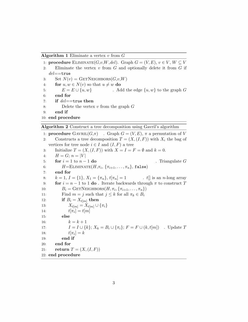
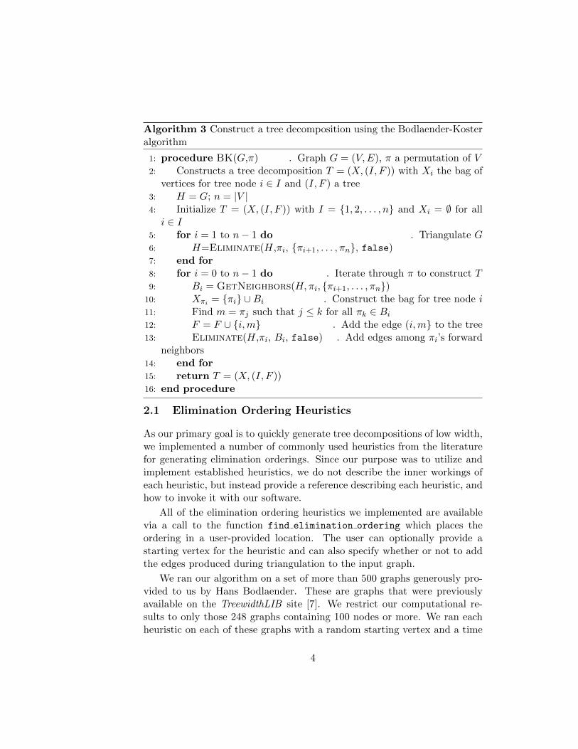
Most computational work has been done utilizing heuristics which offerno guarantee on their maximum deviation from optimality. One of the mostcommon methods for constructing tree decompositions is based on known al-gorithms for decomposing chordal graphs, which are characterized by havingno induced cycles of length greater than three. An elimination ordering is apermutation of the vertex set of a graph, commonly used to guide the addi-tion of edges to make the graph chordal, a process known as triangulation.A valid tree decomposition for the triangulated graph can be formed withbags consisting of the sets of higher numbered neighbors for each vertex inthe elimination ordering. Since a tree decomposition for a graph is valid forall subgraphs on the same vertex set, this simultaneously yields a decompo-sition for the original graph. The specifics of these kinds of procedures arewell-known in the literature and we provide pseudocode of our implemen-tations of two algorithms that create tree decompositions for a graph givenan ordering of its vertices. We require a function GetNeighbors(G, v,W )that returns the neighbors of vertex v in the graph that are also contained inthe set of vertices W . Algorithm 1 describes the elimination of a vertex froma graph, and Algorithm 2 describes the details of our implementation of thetree decomposition construction algorithm outlined in [12]. We describe ourimplementation of the procedure given in [9] in Algorithm 3.

2

Algorithm 1 Eliminate a vertex v from G

1: procedure Eliminate(G,v,W ,del). Graph G = (V,E), v ∈ V , W ⊆ V2: Eliminate the vertex v from G and optionally delete it from G if

del==true

3: Set N(v) = GetNeighbors(G,v,W )4: for u,w ∈ N(v) so that u 6= w do5: E = E ∪ {u,w} . Add the edge {u,w} to the graph G6: end for7: if del==true then8: Delete the vertex v from the graph G9: end if

10: end procedure

Algorithm 2 Construct a tree decomposition using Gavril’s algorithm

1: procedure Gavril(G,π) . Graph G = (V,E), π a permutation of V2: Constructs a tree decomposition T = (X, (I, F )) with Xi the bag of

vertices for tree node i ∈ I and (I, F ) a tree3: Initialize T = (X, (I, F )) with X = I = F = ∅ and k = 0.4: H = G; n = |V |5: for i = 1 to n− 1 do . Triangulate G6: H=Eliminate(H,πi, {πi+1, . . . , πn}, false)7: end for8: k = 1, I = {1}, X1 = {πn}, t[πn] = 1 . t[] is an n-long array9: for i = n− 1 to 1 do . Iterate backwards through π to construct T

10: Bi = GetNeighbors(H,πi, {πi+1, . . . , πn})11: Find m = j such that j ≤ k for all πk ∈ Bi12: if Bi = Xt[m] then13: Xt[m] = Xt[m] ∪ {πi}14: t[πi] = t[m]15: else16: k = k + 117: I = I ∪ {k}; Xk = Bi ∪ {πi}; F = F ∪ (k, t[m]) . Update T18: t[πi] = k19: end if20: end for21: return T = (X, (I, F ))22: end procedure

3

Algorithm 3 Construct a tree decomposition using the Bodlaender-Kosteralgorithm

1: procedure BK(G,π) . Graph G = (V,E), π a permutation of V2: Constructs a tree decomposition T = (X, (I, F )) with Xi the bag of

vertices for tree node i ∈ I and (I, F ) a tree3: H = G; n = |V |4: Initialize T = (X, (I, F )) with I = {1, 2, . . . , n} and Xi = ∅ for alli ∈ I

5: for i = 1 to n− 1 do . Triangulate G6: H=Eliminate(H,πi, {πi+1, . . . , πn}, false)7: end for8: for i = 0 to n− 1 do . Iterate through π to construct T9: Bi = GetNeighbors(H,πi, {πi+1, . . . , πn})

10: Xπi = {πi} ∪Bi . Construct the bag for tree node i11: Find m = πj such that j ≤ k for all πk ∈ Bi12: F = F ∪ {i,m} . Add the edge (i,m} to the tree13: Eliminate(H,πi, Bi, false) . Add edges among πi’s forward

neighbors14: end for15: return T = (X, (I, F ))16: end procedure

2.1 Elimination Ordering Heuristics

As our primary goal is to quickly generate tree decompositions of low width,we implemented a number of commonly used heuristics from the literaturefor generating elimination orderings. Since our purpose was to utilize andimplement established heuristics, we do not describe the inner workings ofeach heuristic, but instead provide a reference describing each heuristic, andhow to invoke it with our software.

All of the elimination ordering heuristics we implemented are availablevia a call to the function find elimination ordering which places theordering in a user-provided location. The user can optionally provide astarting vertex for the heuristic and can also specify whether or not to addthe edges produced during triangulation to the input graph.

We ran our algorithm on a set of more than 500 graphs generously pro-vided to us by Hans Bodlaender. These are graphs that were previouslyavailable on the TreewidthLIB site [7]. We restrict our computational re-sults to only those 248 graphs containing 100 nodes or more. We ran eachheuristic on each of these graphs with a random starting vertex and a time

4

Best Worst Avg. Best WorstHeuristic Avg. Width Width Width Time Time Time Avg.

[Reference] Width Rank Rank Rank Rank Rank Rank TimeMinDegree [13] 72.3 1 9 3.94 1 6 3.42 0.17

MCS [5] 78.95 1 10 7.38 4 10 6.81 205.1MCS-M [5] 105.11 1 10 8.41 1 10 8.35 186.70LEX-M [24] 99.4 1 10 8.37 1 7 9.52 232.8MinFill [14] 66.7 1 7 1.53 4 10 7.83 21.4

MetisMMD [18, 20] 69.75 1 9 3.04 1 8 2.23 0.04MetisNodeND [18] 71.91 1 10 5.12 1 8 2.56 0.05

AMD [2] 72.1 1 10 3.9 1 7 1.85 0.03MMD [20] 72 1 10 4.07 1 6 3.93 0.18

MinMaxDegree 72 1 10 6.83 3 10 6.84 28.6

Table 1: A comparison of the performance of elimination ordering heuristicson a set of test graphs

limit of 7200 seconds. For each run, we recorded the running time (in sec-onds) and the width of the resulting tree decomposition. Table 1 presents theresults of these computational experiments. For each heuristic, we provide areference from the literature and its performance in terms of both width andrunning time. The average width and running times are computed across all248 decompositions. For the width and running time rankings, we providethe best, worst, and average ranking of each heuristic in terms of both widthand running time where a ranking of one indicates the heuristic is the topperformer and a rank of ten means it is the worst. As an example of howto interpret the results, in terms of width, the MinDegree heuristic was thetop-ranked heuristic on at least one problem, it was ranked as low as ninthon one instance, and its average width ranking was 3.94.

We can view the relative performance of each heuristic on this set ofbenchmark graphs by plotting the average width and running time rankingsin the width-time plane. In Figure 1, we see that Greedy Minimum Fill,Metis MMD, and Approximate Minimum Degree (AMD) are not dominatedby any other heuristic in either dimension. If one requires a decompositionwith as small a width as possible, then Greedy Minimum Fill is a goodchoice. For larger graphs where running time becomes an issue, then thebest choices are probably Metis MMD or Approximate Minimum Degree.While the slower, more complex heuristics such as LEXM performed poorlyon many of the problems, we have seen cases where they dramatically out-performs all the other heuristics. For example, on the problem 1dc.256from the DIMACS Independent Set Challenge [26], the LEXM heuristicproduces a decomposition with width 78. However, Greedy Minimum Fill,Metis MMD, and Approximate Minimum Degree produce widths of 119, 132,and 128, respectively. Thus, while Greedy Minimum Fill, Metis MMD, andApproximate Minimum Degree are superior on most instances, exceptionsexist where the other heuristics produce decompositions with much lower

5

MINDMINDMMDMMD

MINFMINF

METMMDMETMMDMETNNDMETNND

AMDAMD

MMAXMMAX

MCSMMCSM

MCSMCS

LEXMLEXM

0 2 4 6 8 10

Mean Width

Rank0

2

4

6

8

10

Mean

Running Time

Rank

Figure 1: A comparison of the average width and average running time ofvarious heuristics on a large set of benchmark problems

widths.

3. Solving Maximum Weighted Independent Set

Having described how to construct tree decompositions, we now describehow we use these decompositions as part of a dynamic programming algo-rithm to solve maximum weighted independent set (MWIS). The dynamicprogramming recursion for using tree decompositions to solve MWIS is well-known [6, 9]. The general idea is to root the tree decomposition and workupwards from the leaves, maintaining a dynamic programming table at eachnode in the tree. Given a tree node j, we denote its bag of vertices asXj and let Gj denote the subgraph induced by all the vertices containedin bags at or beneath tree node j in the rooted tree decomposition. Foreach independent set U ⊆ Xj , there is a table entry with value fj(U) equalto the weight of the maximum weight independent set S ⊆ Gj such thatS ∩Xj = U . Since Gr = G, the largest value in the table for the root noder gives the weight of the maximum weight independent set in G. We nowbriefly describe the computation of fr(U) via dynamic programming.

For a leaf node l in the tree and an independent set U ⊆ Xl, the value offl(U) is just the actual weight w(U) of U since there are no vertices outsideof Xl ⊆ Gl to consider. For a non-leaf node j with d child nodes c1, c2, . . . , cdand some independent set U ⊆ Xj , fj(U) can be calculated in terms of the

6

values stored at the child nodes via the dynamic programming equation

fj(U) = w(U) +d∑i=1

max{fci(V )− w(V ∩ U) : V ∩Xj = U ∩Xci}. (1)

In other words, for every independent set U ⊆ Xj , we must look at thetable for each child tree node ci to find all independent sets V ⊆ Xci thatcontain the same vertices as U from Xci∩Xj . To compute the value of fj(U)we need to find the set V that has the largest value when one excludes theirintersection.

There are two fundamental operations required in this dynamic pro-gramming recursion. First, we must have a fast method for finding all theindependent sets in a bag of vertices. Second, for every independent set Uthat we find in a child node ci, we must store it in such a way that thelookups required to compute equation (1) at the parent can be done veryquickly. We describe the implementation of these operations in the nextsection.

3.1 Implementation Details

3.1.1 Set operations

The most important low-level operations in the dynamic programming al-gorithm are set operations: finding the intersection or union of two setsand checking if a particular vertex is in a set. For performance to be com-petitive with other methods on large problems, these operations must beperformed quickly and in a memory-efficient manner. Since we are al-ways dealing with subsets of a known set (typically a bag of vertices inthe tree decomposition), we are able to represent subsets of vertices as bitvectors and perform the intersection, union, and containment operationsvia bitwise AND (∧) and OR (∨) operations. As an example, supposewe have some bag of vertices B = {2, 4, 6, 8, 10, 11, 12, 15} and two subsetsS, T ⊂ B with S = {2, 8, 10, 15} and T = {4, 6, 10, 11, 15}. The set S isrepresented as 10011001 and T as 01101101. To check if the i-th vertex ofB is in S, we check to see if S ∧ (2i) is non-zero. To calculate the unionS∪T = {2, 4, 6, 8, 10, 11, 15}, we compute 10011001∨01101101 = 11111101.

When a tree decomposition has width less than the processor’s word size(typically 32- or 64-bits), each of these bitwise operations can be done usinga single CPU instruction. For larger width decompositions, we developed abigint t type to represent the required larger bitmasks as an array of 32-

7

or 64-bit words. The code for the bigint t type is included in our softwaredistribution and allows us to handle decompositions with arbitrarily largewidths, as long as memory is available.

3.1.2 Finding all independent sets

A fundamental kernel in the dynamic programming algorithm for MWIS isfinding all the independent sets in a graph. In particular, for each bag ofvertices Xj in the tree decomposition, we must find all the independent setsin the subgraph induced by Xj . As there are 2|Xj | sets to consider, it isclear that this search must be done efficiently, especially for larger widths.Algorithm 4 provides pseudocode for our implementation of this procedure,which takes advantage of the bitwise representation of subsets.

In Algorithm 4, we create a list S of all the independent sets containedin a graph G = (V,E) with n vertices. The sets are represented by thebitmasks s that range from 0 (representing the empty set) up to 2n − 1(representing all of V ). In line 9 we check to see if there is some edge inthe current set s that prevents it from being independent. When we finda non-independent set s′, then in line 18 we are often able to advance thecurrent value of s by a large amount. For example, if we know that thebitmask 1100100 does not represent an independent set, then any mask ofthe form 11001·· cannot represent an independent set. This allows us toadvance to the bitmask 1101000 in the loop by adding 100 to 1100100.

3.1.3 Memory-efficient storage

We now describe our storage methods that allow for efficient lookups whenperforming the dynamic programming recursion. Since we root the tree priorto beginning the dynamic programming, the parent-child relationship of allnodes in the tree is completely known when we search for independent setsand update the tables. As all of the operations required by the dynamicprogramming equation (1) involve the intersection of an independent setwith its parent tree node’s bag, we do not need an entry in the table of treenode i for every independent set U ⊆ Xi. In particular, if j is the parentof tree node i, then we have an entry in i’s table only for the independentsets in Xi ∩ Xj , reducing the amount of storage required by the dynamicprogramming tables.

Nevertheless, when processing a tree node j that has child node ci, forevery independent set U ⊆ Xj , we must still quickly find the entry for U∩Xci

in the table for tree node ci. Since all sets are represented as bitmasks, the

8

Algorithm 4 Find all the weighted independent sets in a graph G = (V,E)

1: procedure FindAllWIS(G)2: Let A be the adjacency matrix of G so that that the row A[i] is

a bitmask representing i’s neighbors and let W [i] denote the weight ofvertex i

3: S = {(∅, 0)}; n = |V |; s = 1 . Store the empty set with weight 04: while s < 2n − 1 do . Loop over all non-empty subsets5: is independent=true; i = w = 06: while i < n and is independent do7: if bit i is set in s then . Vertex i is in the current set s8: w = w +W [i] . Update the weight w of the current set s9: if s ∧A[i] then . s contains some edge (i, ·)

10: is independent=false

11: end if12: end if13: i = i+ 1 . Consider the next vertex in V14: end while15: if is independent then16: S = S ∪ (s, w); s = s+ 1 . Add the set and consider next

bitmask17: else . Jump over 2b non-independent sets18: s = s+ 2b (b the least significant bit of s)19: end if20: end while21: return S22: end procedure

natural solution to this problem is to utilize hash tables. As the width of ourdecompositions grow, the dynamic programming tables can occupy a greatdeal of memory, and so it is essential for the hash table implementation tobe fast and lightweight. Rather than attempt to write our own hash, weexperimented with several well-known existing implementations, includingthe Standard Template Library (STL) map and unordered map as well asthe Boost hashtable. However, in our experience all of these consumed fartoo much memory to handle larger width graphs, and we settled upon afast, open source, macro-based implementation called uthash[15]. This hasproved to be much faster and very robust, allowing us to handle decomposi-tions with much larger widths than alternative hash table implementations.

9

3.1.4 Dynamic programming implementation

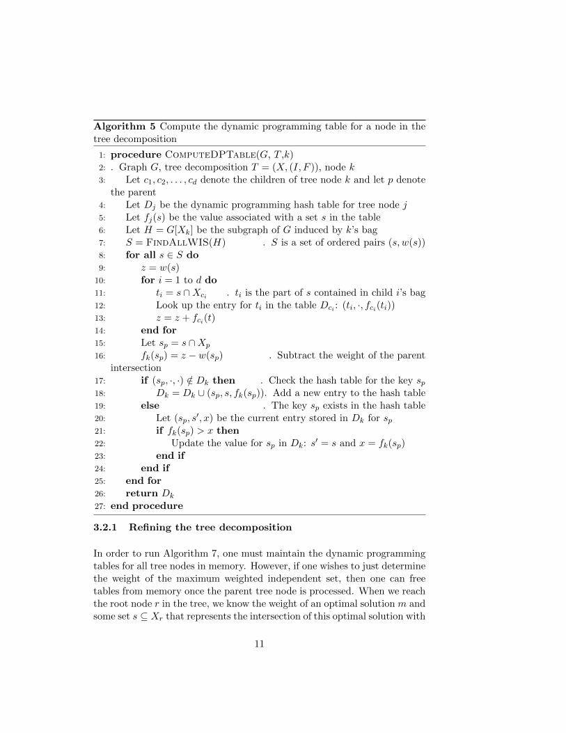
We now provide the details of our dynamic programming implementationfor solving MWIS. Algorithm 5 describes how we compute the dynamicprogramming tables at each node in the tree. In line 7, we generate a listof all the independent sets contained in the subgraph induced by Xk, thebag associated with tree node k. In practice, we do not actually store thislist but instead process each set as it is encountered for a slight savings inmemory. For each independent set s discovered, we compute its value inthe dynamic programming table in line 16 and then incorporate s into thetable Dk in lines 17-24. Note that for each independent set, we store thetriple (sp, s, fk(sp)) where sp is the intersection of s with the parent bag,and fk(sp) is the value associated with this set in the dynamic programmingtable. The bitmask for s is stored as it enables the reconstruction of thefull solution. However, this storage is not necessary if one wishes to simplydetermine the optimal weight.

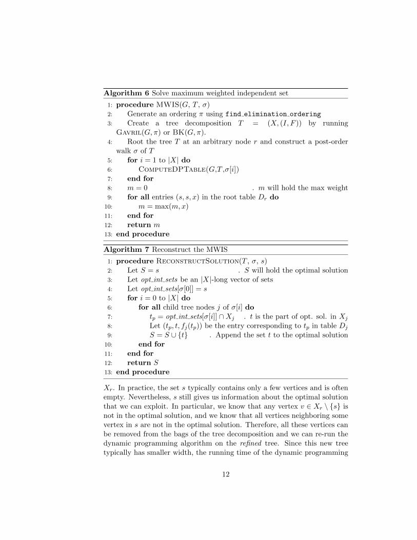
Having described how we compute the dynamic programming table foreach tree node j, it is now straightforward to solve MWIS for an input graph.Algorithm 6 returns the weight m of the maximum weighted independent setinG. However, it typically only gives us limited information about the actualoptimal solution discovered since the entry (s, s,m) in the tableDr only givesus the vertices in this solution that are contained in the bag Xr. The actualsolution itself can be reconstructed very quickly by descending back downthe tree starting at the root node. Given a pre-order walk σ of the rootedtree decomposition, and the set s that represents this solution’s intersectionwith the root node’s bag, Algorithm 7 describes how to reconstruct thecorresponding actual optimal solution that has weight m.

3.2 Memory Usage

The obvious bottleneck for the dynamic programming algorithm is the stor-age of the hash tables Dk at each tree node k. As mentioned previously,one way we reduce the memory requirements is by storing a single entry(sp, s, fk(sp)) for each independent set sp in the intersection of a tree node’sbag with its parent’s. Nevertheless, the memory usage for our algorithmcan still be extremely large. Below we describe another optimization thatproved to be quite beneficial in practice.

10

Algorithm 5 Compute the dynamic programming table for a node in thetree decomposition

1: procedure ComputeDPTable(G, T ,k)2: . Graph G, tree decomposition T = (X, (I, F )), node k3: Let c1, c2, . . . , cd denote the children of tree node k and let p denote

the parent4: Let Dj be the dynamic programming hash table for tree node j5: Let fj(s) be the value associated with a set s in the table6: Let H = G[Xk] be the subgraph of G induced by k’s bag7: S = FindAllWIS(H) . S is a set of ordered pairs (s, w(s))8: for all s ∈ S do9: z = w(s)

10: for i = 1 to d do11: ti = s ∩Xci . ti is the part of s contained in child i’s bag12: Look up the entry for ti in the table Dci : (ti, ·, fci(ti))13: z = z + fci(t)14: end for15: Let sp = s ∩Xp

16: fk(sp) = z − w(sp) . Subtract the weight of the parentintersection

17: if (sp, ·, ·) /∈ Dk then . Check the hash table for the key sp18: Dk = Dk ∪ (sp, s, fk(sp)). Add a new entry to the hash table19: else . The key sp exists in the hash table20: Let (sp, s

′, x) be the current entry stored in Dk for sp21: if fk(sp) > x then22: Update the value for sp in Dk: s

′ = s and x = fk(sp)23: end if24: end if25: end for26: return Dk

27: end procedure

3.2.1 Refining the tree decomposition

In order to run Algorithm 7, one must maintain the dynamic programmingtables for all tree nodes in memory. However, if one wishes to just determinethe weight of the maximum weighted independent set, then one can freetables from memory once the parent tree node is processed. When we reachthe root node r in the tree, we know the weight of an optimal solution m andsome set s ⊆ Xr that represents the intersection of this optimal solution with

11

Algorithm 6 Solve maximum weighted independent set

1: procedure MWIS(G, T , σ)2: Generate an ordering π using find elimination ordering

3: Create a tree decomposition T = (X, (I, F )) by runningGavril(G, π) or BK(G, π).

4: Root the tree T at an arbitrary node r and construct a post-orderwalk σ of T

5: for i = 1 to |X| do6: ComputeDPTable(G,T ,σ[i])7: end for8: m = 0 . m will hold the max weight9: for all entries (s, s, x) in the root table Dr do

10: m = max(m,x)11: end for12: return m13: end procedure

Algorithm 7 Reconstruct the MWIS

1: procedure ReconstructSolution(T , σ, s)2: Let S = s . S will hold the optimal solution3: Let opt int sets be an |X|-long vector of sets4: Let opt int sets[σ[0]] = s5: for i = 0 to |X| do6: for all child tree nodes j of σ[i] do7: tp = opt int sets[σ[i]] ∩Xj . t is the part of opt. sol. in Xj

8: Let (tp, t, fj(tp)) be the entry corresponding to tp in table Dj

9: S = S ∪ {t} . Append the set t to the optimal solution10: end for11: end for12: return S13: end procedure

Xr. In practice, the set s typically contains only a few vertices and is oftenempty. Nevertheless, s still gives us information about the optimal solutionthat we can exploit. In particular, we know that any vertex v ∈ Xr \ {s} isnot in the optimal solution, and we know that all vertices neighboring somevertex in s are not in the optimal solution. Therefore, all these vertices canbe removed from the bags of the tree decomposition and we can re-run thedynamic programming algorithm on the refined tree. Since this new treetypically has smaller width, the running time of the dynamic programming

12

Figure 2: The maximum independent set in the graph is {A,D,F,H}, andA is the only vertex in this set also in the root node. Therefore, B and Ccan be removed from the tree decomposition in the refinement procedure.

algorithm on the new tree is exponentially smaller, and the tables requiremuch less space, allowing us to store them in memory in order to reconstructthe solution.

3.2.2 Memory usage estimation

Even with the refined tree, the memory required to process a single treenode can still be too large, so we analyzed the memory consumption inmore detail. Given a tree node i and its parent p, we have a single entry foreach independent set contained in the intersection of Y = Xi ∩Xp. Whenthe relevant subgraph induced by Y is very sparse, there can be O(2|Y |)independent sets to store, and so the memory consumption can truly beexponential in the size of Y . However, the density of the subgraph plays acritical role in the actual expected number of independent sets contained insuch a subgraph.

Under a few basic assumptions, we can estimate the expected total num-ber of independent sets contained in a subgraph and use this to determineif a tree decomposition-based approach is tractable. Given some set Y asabove, let H be the subgraph induced by Y . Denote the number of verticesin H as w and the number of edges as s and assume that the probabilityof any two vertices in H being joined by an edge is the same for all pairsof vertices. Then the probability of any two vertices u, v in H not beingjoined by an edge is ρ = 1− s/

(w2

), and so the probability that some set of q

vertices from Y represents an independent set is ρ(q2). The expected numberof independent sets in H is then

E[|FindAllWIS(H)|] = 1 +w∑k=1

(w

k

)ρ(k2). (2)

13

We were unable to determine an asymptotic formula for equation (2), butwe can compute the sum directly. Our software is able to compute thisvalue exactly using multiple precision arithmetic, and in the next section wedemonstrate that it is typically a very good estimate of the number of inde-pendent sets found and stored over the course of the dynamic programmingalgorithm implementation.

4. Computational Results

Our goals are to compare the overall performance of our dynamic program-ming algorithm with other well-established methods, to explore how ouralgorithm’s performance scales as we alter various properties of the graphs,and to examine the traditional wisdom regarding the maximum width graphsthat can be handled via tree decomposition-based dynamic programming.All of the experiments in this section were conducted using a standard Linuxcompute node equipped with 16GB of RAM and two quad-core AMD pro-cessors.

4.1 Partial k-trees

One of the challenges in analyzing the performance of our algorithms wasfinding a suitable set of graphs with a wide variety of sizes and densities withknown upper bounds on the treewidth. Fortunately, it is straightforward togenerate such graphs, using the definition of partial k-trees. The class of k-trees is defined recursively. In the smallest case, a clique on k+1 vertices is ak-tree. Otherwise, for n > k, a k-tree G on n+1 vertices can be constructedfrom a k-tree H on n vertices by adding a new vertex v adjacent to someset of k vertices which form a clique in H. A k-tree has treewidth exactly k(the bags of the optimal tree decomposition are the cliques of size k + 1).The set of all subgraphs of k-trees is known as the partial k-trees. It easyto see that any partial k-tree has treewidth at most k (one can derive avalid tree decomposition of width k from that of the k-tree which containsit). Furthermore, any graph with treewidth at most k is the subgraph ofsome k-tree [19]. Thus the set of all graphs with treewidth at most k canbe generated by finding all k-trees and their subgraphs, leading us to aneasy randomized generator for graphs of bounded treewidth. The INDDGOsoftware distribution includes an executable, gen pkt, to produce randomlygenerated partial k-trees.

14

æ æ æ æ æ æ æ æ æ æ æ æ æ æ æ æ æ æ æ æ æ æ æ æ æ æ æ æ æ æ æ æ æ æ æ æ æ æ æ æ æ

à à à à à à à à à à à à àà à à à à

à à à à à à à à à à à à à à à à à à àà à à àì

ì

ì ì ì ì

ì

ì ì ì ì ìì ì ì ì ì ì ì ì ì ì ì ì ì ì ì ì ì ì ì ì ì ì ì ì ì

ì ì ì ì

ò ò ò ò ò ò ò ò ò ò ò ò ò ò ò ò ò ò ò ò ò ò ò ò ò ò ò ò ò ò ò

òò ò

ò

ò

ò ò

ò

ò

ò

20 30 40 50Width

100

200

300

400

Running Time

ò INDDGO

ì BPM

à IPM

æ Gurobi

ææ æ æ

ææ

æ

ææ æ æ æ

ææ

ææ æ æ æ æ æ æ æ æ æ

ææ æ æ æ æ æ æ æ æ æ æ æ æ æ æ

à à à à à à à à à à à à àà à à à à

à à à à à à à à à à à à à à à à à à à à à à à

ì

ì

ì ì ì ì

ì

ì ì ì ì ì ì ì ì ì ì ì ì ì ì ì ì ì ì ì ì ì ì ì ì ì ì ì ì ì ì ì ì ì ì

ò ò ò ò ò ò ò ò òò ò

òò

ò ò ò ò

ò

ò ò

ò

ò

ò

ò ò

òò

ò

ò òò

ò ò ò

ò

ò

òò

ò ò

ò

20 30 40 50Width

8

10

12

14

16LogHmemoryL

ò INDDGO

ì BPM

à IPM

æ Gurobi

Figure 3: The running time and memory usage of the other methods re-main roughly constant as the width varies while n and m remain constant.The tree decomposition based approach requires more memory as the widthincreases.

4.2 Comparison with other algorithms

We compared the runtime and memory usage of our algorithm against otherwell-known implementations: the commercial mixed integer programmingsolver, Gurobi, and two freely available branch and bound algorithms forMWIS based on the semi-definite programming (SDP) relaxation [10]. Oneof the SDP-based codes uses an interior point method (IPM ) to solve theSDP, and the other uses a boundary point method (BPM ).

For experiments with Gurobi, we formulate the MWIS instance as apure 0/1 integer programming (IP) problem and then produce an input filethat is read directly by Gurobi. The two implementations based on theSDP relaxation are able to read problem instances directly from so-calledDIMACS files [26] so that no translation is necessary. Before presenting theresults, we note that it is not our intention to claim superiority of any oneimplementation over another. Instead, we are primarily interested in thescaling behavior of each implementation in terms of the size of the instance,measured in terms of the number of nodes, number of edges, or width of agiven tree decomposition.

In our first computational experiment, we generated a set of 40 partialk-trees. Each of these graphs has 256 nodes and approximately 2056 edges,with k running from 11 to 50 and p (the probability of keeping an edge inthe k-tree) varying from 0.17 to 0.81. We created tree decompositions us-ing the Greedy Minimum Fill heuristic and Gavril’s algorithm, and ran ourdynamic programming algorithm along with the SDP codes and Gurobi. InFigure 3, we see that the running time and memory usage of our dynamicprogramming are in line with the other methods until we reach the graphs

15

Number Avg. Max Avg. MaxImplementation Completed Time Time Mem (GB) Mem(GB)

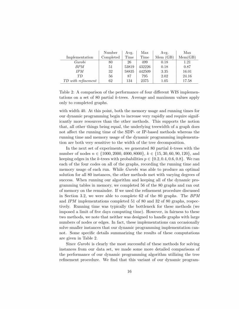
Gurobi 80 26 499 0.18 1.21BPM 51 53819 432226 0.18 0.87IPM 32 58835 442509 3.35 16.01TD 56 87 795 2.02 24.16

TD with refinement 62 134 2375 1.05 17.58

Table 2: A comparison of the performance of four different WIS implemen-tations on a set of 80 partial k-trees. Average and maximum values applyonly to completed graphs.

with width 40. At this point, both the memory usage and running times forour dynamic programming begin to increase very rapidly and require signif-icantly more resources than the other methods. This supports the notionthat, all other things being equal, the underlying treewidth of a graph doesnot affect the running time of the SDP- or IP-based methods whereas therunning time and memory usage of the dynamic programming implementa-tion are both very sensitive to the width of the tree decomposition.

In the next set of experiments, we generated 80 partial k-trees with thenumber of nodes n ∈ {1000, 2000, 4000, 8000}, k ∈ {15, 30, 60, 90, 120}, andkeeping edges in the k-trees with probabilities p ∈ {0.2, 0.4, 0.6, 0.8}. We raneach of the four codes on all of the graphs, recording the running time andmemory usage of each run. While Gurobi was able to produce an optimalsolution for all 80 instances, the other methods met with varying degrees ofsuccess. When running our algorithm and keeping all of the dynamic pro-gramming tables in memory, we completed 56 of the 80 graphs and ran outof memory on the remainder. If we used the refinement procedure discussedin Section 3.2, we were able to complete 62 of the 80 graphs. The BPMand IPM implementations completed 51 of 80 and 32 of 80 graphs, respec-tively. Running time was typically the bottleneck for these methods (weimposed a limit of five days computing time). However, in fairness to thesetwo methods, we note that neither was designed to handle graphs with largenumbers of nodes or edges. In fact, these implementations can occasionallysolve smaller instances that our dynamic programming implementation can-not. Some specific details summarizing the results of these computationsare given in Table 2.

Since Gurobi is clearly the most successful of these methods for solvinginstances from our data set, we made some more detailed comparisons ofthe performance of our dynamic programming algorithm utilizing the treerefinement procedure. We find that this variant of our dynamic program-

16

Gurobi Refined TDn m time memory time memory

1000 17721 0.543 29008 0.54 175282000 35721 1.684 52516 0.99 261044000 71721 4.423 98700 2.76 530408000 143721 19.618 194284 8.72 1012361000 23628 0.764 38348 0.36 94162000 47628 2.35 70140 0.75 170964000 95628 10.424 133872 2.85 306648000 191628 44.986 254920 8.6 56176

Table 3: A comparison of the dynamic programming algorithm versusGurobi on a particular family of partial k-trees with k = 30 and p = .8.

ming implementation can be up to 5 times faster than Gurobi on certaingraphs. A more detailed inspection of the results shows that our implemen-tation is faster on all partial k-trees in our test set with k = 15 or 30 andp = 0.6 or p = 0.8. These are lower width instances that share the majorityof edges with the original k-tree. Since each bag in the tree decompositionof these graphs is somewhat dense, equation (2) implies that the dynamicprogramming tables remain small, leading to lower memory usage and fasterrunning times. Table 3 contains some more detailed information regardingthe instances with k = 30 and p = 0.8. It is worth noting that on all ofthese instances where our running time is lower, our memory usage is alsosubstantially less than Gurobi ’s.

4.3 Results on large width graphs

Due to the theoretical exponential growth in running time and memoryusage, the traditional thinking has been that graphs with larger widthscannot be handled by dynamic programming based on tree decompositions.For example, Huffner, et al, [17] state that “As a rule of thumb, the typicalborder of practical feasibility lies somewhere below a treewidth of 20 for theunderlying graph.” In this section, we run our algorithm on a particular classof partial k-trees where we increase the parameter k as much as possible.This allows us to find the optimal solution to weighted independent setinstances on graphs with 10,000 nodes where the width of the underlyingdecomposition is as large as 708.

For this experiment, we generated partial k-trees with 10,000 nodes,p = 0.9 and k ∈ {100, 200, . . . , 700}. The resulting seven graphs have up to

17

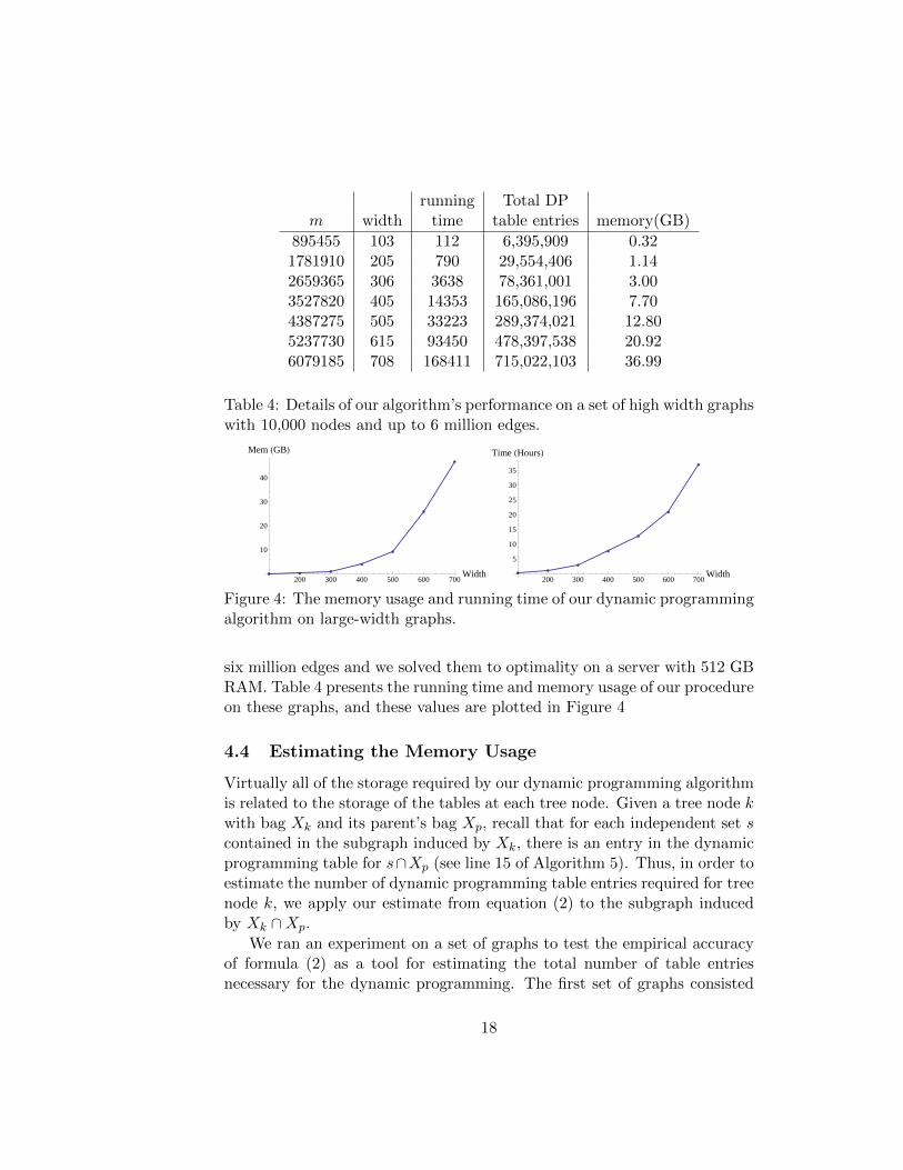
running Total DPm width time table entries memory(GB)

895455 103 112 6,395,909 0.321781910 205 790 29,554,406 1.142659365 306 3638 78,361,001 3.003527820 405 14353 165,086,196 7.704387275 505 33223 289,374,021 12.805237730 615 93450 478,397,538 20.926079185 708 168411 715,022,103 36.99

Table 4: Details of our algorithm’s performance on a set of high width graphswith 10,000 nodes and up to 6 million edges.

æ ææ

æ

æ

æ

æ

200 300 400 500 600 700Width

10

20

30

40

Mem HGBL

ææ

æ

æ

æ

æ

æ

200 300 400 500 600 700Width

5

10

15

20

25

30

35

Time HHoursL

Figure 4: The memory usage and running time of our dynamic programmingalgorithm on large-width graphs.

six million edges and we solved them to optimality on a server with 512 GBRAM. Table 4 presents the running time and memory usage of our procedureon these graphs, and these values are plotted in Figure 4

4.4 Estimating the Memory Usage

Virtually all of the storage required by our dynamic programming algorithmis related to the storage of the tables at each tree node. Given a tree node kwith bag Xk and its parent’s bag Xp, recall that for each independent set scontained in the subgraph induced by Xk, there is an entry in the dynamicprogramming table for s∩Xp (see line 15 of Algorithm 5). Thus, in order toestimate the number of dynamic programming table entries required for treenode k, we apply our estimate from equation (2) to the subgraph inducedby Xk ∩Xp.

We ran an experiment on a set of graphs to test the empirical accuracyof formula (2) as a tool for estimating the total number of table entriesnecessary for the dynamic programming. The first set of graphs consisted

18

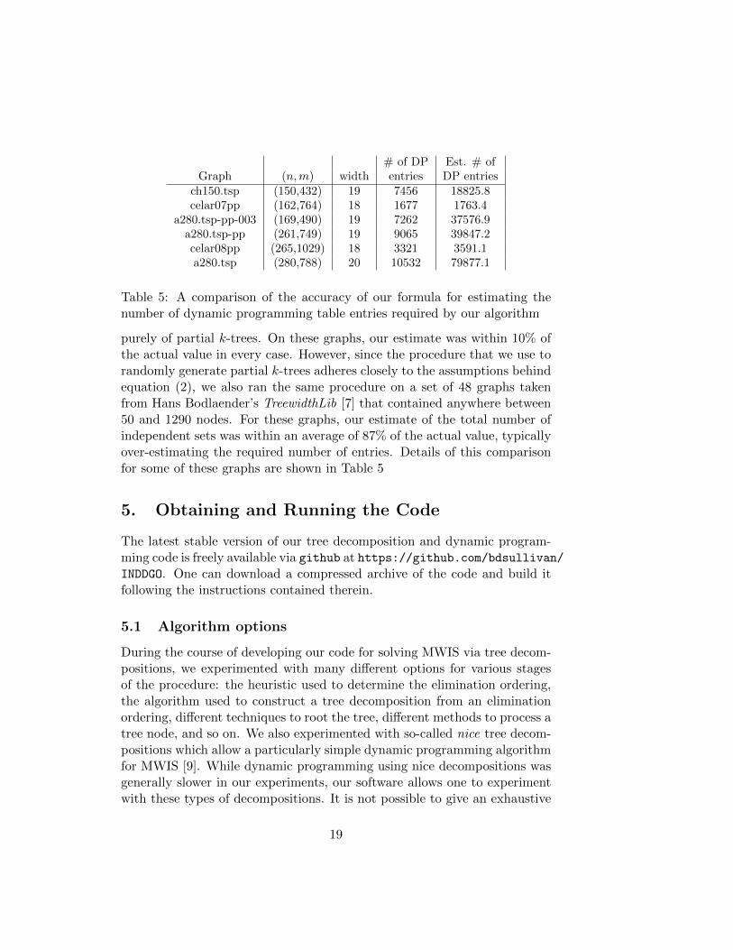
# of DP Est. # ofGraph (n,m) width entries DP entries

ch150.tsp (150,432) 19 7456 18825.8celar07pp (162,764) 18 1677 1763.4

a280.tsp-pp-003 (169,490) 19 7262 37576.9a280.tsp-pp (261,749) 19 9065 39847.2celar08pp (265,1029) 18 3321 3591.1a280.tsp (280,788) 20 10532 79877.1

Table 5: A comparison of the accuracy of our formula for estimating thenumber of dynamic programming table entries required by our algorithm

purely of partial k-trees. On these graphs, our estimate was within 10% ofthe actual value in every case. However, since the procedure that we use torandomly generate partial k-trees adheres closely to the assumptions behindequation (2), we also ran the same procedure on a set of 48 graphs takenfrom Hans Bodlaender’s TreewidthLib [7] that contained anywhere between50 and 1290 nodes. For these graphs, our estimate of the total number ofindependent sets was within an average of 87% of the actual value, typicallyover-estimating the required number of entries. Details of this comparisonfor some of these graphs are shown in Table 5

5. Obtaining and Running the Code

The latest stable version of our tree decomposition and dynamic program-ming code is freely available via github at https://github.com/bdsullivan/INDDGO. One can download a compressed archive of the code and build itfollowing the instructions contained therein.

5.1 Algorithm options

During the course of developing our code for solving MWIS via tree decom-positions, we experimented with many different options for various stagesof the procedure: the heuristic used to determine the elimination ordering,the algorithm used to construct a tree decomposition from an eliminationordering, different techniques to root the tree, different methods to process atree node, and so on. We also experimented with so-called nice tree decom-positions which allow a particularly simple dynamic programming algorithmfor MWIS [9]. While dynamic programming using nice decompositions wasgenerally slower in our experiments, our software allows one to experimentwith these types of decompositions. It is not possible to give an exhaustive

19

1

2

3

6

4

125

7

8

9

10

11

13

20

14

21

19

15

16

17

18

22

23

24

25

1

6566

2

71

72

94

3

75

76

102

4127

162

5

151

171

6117

7161

8

163

173

9172

177

1079

80

176

11

83

84

180

12

141

164

13

184

207

14197

209

15

208

211

16

210 214

17

213

217

18

216

221

19

170

20

193

21

206

22220

225

23

224

230

24

229

25

234

67

68

69

70

87

95

103

73

74

118

128

77

78

142

152

81

82

181

185

85

86194

198

8889

90

91

92

93

96

97

98

99

100

101

104

105106

107

108

109

110

111112 113

114

115 116

119120121

122123

124

125

126

129

130

131

132

133

134

135

136

137

138

139

140

143

144

145

146

147

148

149

150

153154

155

156157

158

159

160

165

166

167

168

169

174175

178

179

182 183

186

187

188

189

190

191

192

195196

199

200

201

202

203

204

205

212

215

218219

222

223

226227

228

231

232233

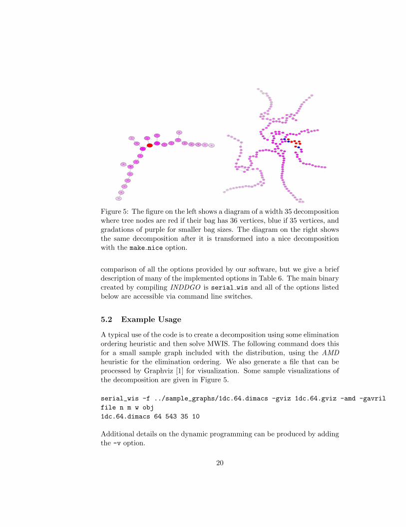
Figure 5: The figure on the left shows a diagram of a width 35 decompositionwhere tree nodes are red if their bag has 36 vertices, blue if 35 vertices, andgradations of purple for smaller bag sizes. The diagram on the right showsthe same decomposition after it is transformed into a nice decompositionwith the make nice option.

comparison of all the options provided by our software, but we give a briefdescription of many of the implemented options in Table 6. The main binarycreated by compiling INDDGO is serial wis and all of the options listedbelow are accessible via command line switches.

5.2 Example Usage

A typical use of the code is to create a decomposition using some eliminationordering heuristic and then solve MWIS. The following command does thisfor a small sample graph included with the distribution, using the AMDheuristic for the elimination ordering. We also generate a file that can beprocessed by Graphviz [1] for visualization. Some sample visualizations ofthe decomposition are given in Figure 5.

serial_wis -f ../sample_graphs/1dc.64.dimacs -gviz 1dc.64.gviz -amd -gavril

file n m w obj

1dc.64.dimacs 64 543 35 10

Additional details on the dynamic programming can be produced by addingthe -v option.

20

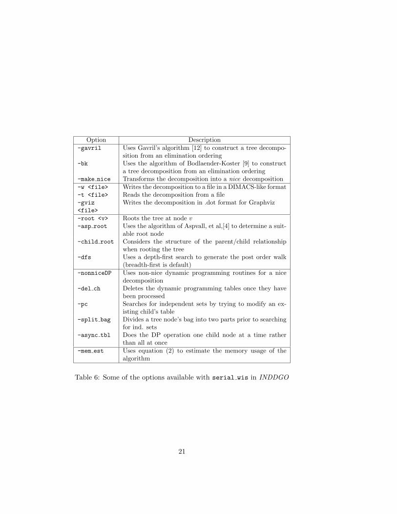
Option Description-gavril Uses Gavril’s algorithm [12] to construct a tree decompo-

sition from an elimination ordering-bk Uses the algorithm of Bodlaender-Koster [9] to construct

a tree decomposition from an elimination ordering-make nice Transforms the decomposition into a nice decomposition-w <file> Writes the decomposition to a file in a DIMACS-like format-t <file> Reads the decomposition from a file-gviz

<file>

Writes the decomposition in .dot format for Graphviz

-root <v> Roots the tree at node v-asp root Uses the algorithm of Aspvall, et al,[4] to determine a suit-

able root node-child root Considers the structure of the parent/child relationship

when rooting the tree-dfs Uses a depth-first search to generate the post order walk

(breadth-first is default)-nonniceDP Uses non-nice dynamic programming routines for a nice

decomposition-del ch Deletes the dynamic programming tables once they have

been processed-pc Searches for independent sets by trying to modify an ex-

isting child’s table-split bag Divides a tree node’s bag into two parts prior to searching

for ind. sets-async tbl Does the DP operation one child node at a time rather

than all at once-mem est Uses equation (2) to estimate the memory usage of the

algorithm

Table 6: Some of the options available with serial wis in INDDGO

21

6. Conclusion

In this paper, we have described an efficient and freely available software li-brary for generating tree decompositions and running dynamic programmingto solve weighted independent set instances. Our software offers easy-to-useimplementations of many well-known heuristics for producing eliminationorderings that lead to low-width tree decompositions. Our dynamic pro-gramming code is particularly memory efficient and computational experi-ments indicate that our implementation is competitive and even superior tostate of the art methods for certain types of MWIS instances. While sparsegraphs with large widths present memory consumption difficulties that ourcode is currently unable to handle, we have nevertheless demonstrated thatdynamic programming on decompositions with very large widths can be fea-sible in some cases, casting doubt on the conventional wisdom. While ourcode currently is able to solve only weighted independent set, our softwareframework is designed so that other dynamic programming algorithms canbe incorporated in a modular fashion. Finally, we mention that we havecreated a parallel version of our software that is able to generate tree de-compositions and solve weighted independent set instances using distributedmemory architectures [27].

7. Acknowledgments

The authors thank the support of the Department of Energy Applied Mathe-matics Program for supporting this work. Additionally, we thank Hans Bod-laender for sending us a large set of test graphs, Arie Koster for sending ushis source code for elimination orderings, Brian Borchers for assistance withbuilding and running the IPM and BMP codes, interns Gloria D’Azevedoand Zhibin Huang for early participation in the project, and Josh Lothianfor helping to organize the code and build procedures.

References

[1] Graphviz, graph visualization software.

[2] P. Amestoy, T. Davis, and I. Duff. ”an approximate minimum degree orderingalgorithm”. ”SIAM J. Matrix Analysis and Applications”, 17:886–905, 1996.

[3] Eyal Amir. Approximation algorithms for treewidth. Algorithmica, page inpress, 2008.

22

[4] Bengt Aspvall, Andrzej Proskurowski, and Jan Arne Telle. Memory require-ments for table computations in partial k-tree algorithms. In Algorithm Theory- SWAT’98, pages 222–233. Springer-Verlag, 1998.

[5] Anne Berry, Jean Blair, Pinar Heggernes, and Barry Peyton. Maximum car-dinality search for computing minimum triangulations of graphs. In ALGO-RITHMICA, pages 1–12. Springer-Verlag, 2002.

[6] A. Bockmayr and K. Reinert. Discrete math for bioinformatics, 2010.

[7] H. Bodlaender. uthash, a benchmark for algorithms for treewidth and relatedgraph problems, 2011.

[8] H. L. Bodlaender. A linear time algorithm for finding tree-decompositions ofsmall treewidth. SIAM Journal of Computing, 25:1305–1317, 1996.

[9] H. L. Bodlaender and A. M. C. A. Koster. Combinatorial optimization ongraphs of bounded treewidth. The Computer Journal, 51(3):245–269, 2008.

[10] B. Borchers and A. Wilson. Branch and bound code for maximum independentset. http://euler.nmt.edu/~brian/mis_bpm/, 2009.

[11] Bruno Courcelle. Graph rewriting: An algebraic and logic approach. In Hand-book of Theoretical Computer Science, Volume B: Formal Models and Seman-tics (B), pages 193–242. 1990.

[12] Fanica Gavril. The intersection graphs of subtrees in trees are exactly thechordal graphs. Journal of Combinatorial Theory, Series B, 16:47–56, 1974.

[13] A. George and J. Liu. The evolution of the minimum degree ordering algorithm.SIAM Review, 31:1–19, 1989.

[14] Vibhav Gogate and Rina Dechter. A complete anytime algorithm for treewidth.In Proceedings of the 20th conference on Uncertainty in artificial intelligence,UAI ’04, pages 201–208, Arlington, Virginia, United States, 2004. AUAI Press.

[15] T. Hanson. uthash, a hash table for c structures,http://uthash.sourceforge.net/, 2011.

[16] I. V. Hicks, A. M. C. A. Koster, and E. Kolotoglu. Branch and tree decompo-sition techniques for discrete optimization. Tutorials in Operations Research,INFORMS–New Orleans, 2005.

[17] Falk Huffner, Rolf Niedermeier, and Sebastian Wernicke. Developing fixed-parameter algorithms to solve combinatorially explosive biological problems.453, May 2008.

[18] G. Karypis. METIS - serial graph partitioning and fill-reducing matrix order-ing, 2011.

[19] T. Kloks. Treewidth: Computations and Approximations. Lecture Notes inComputer Science. Springer, 1994.

23

[20] Joseph Liu. Modification of the minimum-degree algorithm by multiple elimi-nation. ACM Trans. Math. Software, 11:141–153, 1985.

[21] N. Robertson and P. D. Seymour. Graph minors XX: Wagner’s conjecture.Journal of Combinatorial Theory, Series B, 92:325–357, 2004.

[22] Neil Robertson and Paul D. Seymour. Graph minors III: Planar tree-width.Journal of Combinatorial Theory, Ser. B, 36(1):49–64, 1984.

[23] H. Rohrig. Tree decomposition: A feasibility study. Master’s thesis, Max-Planck-Institut fuur Informatik, Saarbruucken, Germany, 1998.

[24] D. Rose, R. Tarjan, and G. Lueker. Algorithmic aspects of vertex eliminationon graphs. SIAM J. Comput., 5:266–283, 1976.

[25] P. D. Seymour and R. Thomas. Call routing and the ratcatcher. Combinator-ica, 14(2):217–241, 1994.

[26] N. Sloane. Challenge problems: Independent sets in graphs, 2011.

[27] Blair D. Sullivan, Dinesh Weerapurage, and Chris Groer. Parallel algorithmsfor graph optimization using tree decompositions. ORNL/TM-2012/194, 2012.

24