Increasing Inventories:

The Role of Sourcing Inputs from China

Maria Jose Carreras Valle∗

August 9, 2021

Abstract

Technological progress and falling trade barriers have allowed firms to create global

value chains. This process allows access to low cost suppliers in other countries, but

leaves firms more exposed to the risks of long delivery times and delivery delays for

their inputs. To insure against these risks, firms can hold costly inventories. This paper

documents the rise in U.S. manufacturing inventories after 2005, and the substitution

of U.S. domestic inputs for inputs from China, which face delivery risk. I build a model

of firms’ decisions to source domestic or foreign inputs and to hold inventories, which

takes into account the relative price of the inputs and the delivery time risk that only

foreign inputs face. I find that 47% of the increase in U.S. manufacturing inventories

is due to an insurance motive for risky input deliveries from China. Additionally,

the paper highlights the importance of delivery time risk in firms’ decisions to create

integrated supply chains. The cost of insurance, measured as the cost of the increase

in inventory stock, is 1.6% of gross output for the period.

Fields: International Economics (primary), Macroeconomics

JEL Classification: F62, F10, F13, F15, D57, D81, L60

∗Ph.D. student at University of Minnesota; email: carre114@umn.edu

1

1 Introduction

Technological progress and falling trade barriers have allowed firms to create global value

chains, fragmenting the production process and locating it across different countries. This

process allows firms to exploit comparative advantage and enables access to low cost suppliers

in other countries. On the other hand, trade is costly and risky. Traded goods have trans-

portation costs, import tariffs, administrative and legal barriers, among other. Firms that

engage in trade face additional risks, such as trade policy uncertainty, political uncertainty,

and the focus of this paper, delivery time risk.

I define delivery time risk as (i) the interaction between long delivery times for the inputs

used in production and any other type of uncertainty the firm is facing, such as demand

changes of productivity shocks, and (ii) delivery delays for their inputs. Delivery time risk

is especially costly in the presence of global supply chains (Hummels and Schaur (2013)).

Even when delivery times can be planned by firms and orders can be placed in advance,

when a firm faces per period demand shocks, long delivery times diminish firm’s ability to

meet their demand every period. Additionally, delivery delays of inputs can stop the entire

production process in the supply chain.

One tool firms have to insure against delivery time risk is to stock up on inventory. This

paper studies the role of inventories as insurance for delivery time risk when firms decide to

source inputs from abroad. I highlight the importance of including delivery time risk when

analyzing the benefits of integrating supply chains, by measuring the cost of insurance using

the change in inventory stock as sourcing decisions change.

This paper makes three main contributions. First, I document the rise in U.S. manufacturing

inventories that started in 2005. Inventories over sales grew 19% from 2005 to 2018. The

increase is observed across manufacturing sectors and types of inventories. Second, I build

a general equilibrium model to study firm’s decision to source domestic and foreign inputs,

2

and their corresponding inventories decisions, where I include delivery time risk only foreign

inputs face. I introduce a new way to model delivery times, which can be adjusted to any

length of time1, which allows to measure how marginal changes of delivery times affect firms

sourcing and inventory decisions.

Third, I use the model to study the rise in U.S. manufacturing inventories over sales through

the increase in U.S. imported inputs from China. Most imports with China arrive via ocean

transportation, which face long delivery times and delays. I find that 47% of the increase in

inventories from 2005 to 2018 is explained by the insurance needs of the added delivery time

risk of sourcing inputs form China. The cost of insurance, measure as the cost of the increase

in inventory stock is 1.6% of gross output in that period, which is significant compared to

the 1.3% increase of gross output.

This paper relies on four main facts. First, it builds on the fact that inventories increase

with imported input intensity (Alessandria et al. (2010a), Vieira Nadais (2017), and Khan

and Khederlarian (2020a)). I show that for aggregate U.S. manufacturing industries, there

is a positive, strong relationship between industries with a high imported input share and

their level of inventories. Second, the total share of imported inputs increased from 13.3%

in 1997 to 16.5% in 2018. The increase shows a substitution of domestic inputs to foreign

inputs, which is driven by the rise in imported inputs from China, which grew from 1.1% in

1997 to 4.1% in 2018.

Third, U.S. trade with China faces high delivery time risk, specially when compared to other

main U.S. trade partners, Mexico and Canada, which are geographically closer. On average,

81% of imports from China are transported via ocean vessel, which take between 25−35 days

to arrive2, and delays are most common for ocean transportation. Last, U.S. manufacturing

inventories represent 13% of gross output3, and have been increasing since 2005 as shown in

1In the literature is more common to find a fixed one period lag for the delivery of inputs.2Data on delivery times from China to U.S. from Freightos website3Mean for 1992-2018.

3

figure 2. The increase is observed across manufacturing industries and types of inventories.

The sharpest rise is observed in intermediate input inventories (defined as work in process

by the U.S. Census Bureau), and are the main focus of this paper.

Figure 1: Increase in U.S. Manufacturing Inventories

11.

21.

41.

61.

8In

vent

ory

over

mon

thly

sal

es

1990m1 2000m1 2010m1 2020m1Monthly data

Figure 2: Monthly manufacturing inventories

Motivated by these facts, I build a general equilibrium model centered in firm’s decision to

demand domestic and foreign inputs to produce, and their corresponding inventory decisions.

Firms take into account the relative price of both inputs and the delivery time risk that only

foreign inputs face. For example, if the price of the foreign input falls, there is a substitution

of domestic to foreign goods, increasing the reliance on foreign inputs and inventories increase

as insurance against the additional risk firms are facing.

The paper proceeds as follows. Section 2 includes the descriptive evidence on U.S. manufac-

turing inventories. Documents the increase in U.S. manufacturing inventories, the increase

in imported inputs from China, and the long delivery times that trade with China faces.

Additionally, it includes the details on data sources used throughout the analysis. Section

3 described the model used to study the response of inventories to integration China to the

supply chain of U.S. manufacturing firms. Section 4 estimates the model for the U.S., and

introduces a measure to quantify the uncertainty associated to the creation of global supply

chains. Section 5 contains the results from the model, and section 6 has robustness checks

4

for the main parameters of the model. Finally, section 7 concludes.

Literature review.

This paper is most closely related to the growing literature on the importance of inventories

in trade. Alessandria et al. (2010a), Alessandria et al. (2010b), and Alessandria et al. (2010c),

explore the relationship between inventories and imports of foreign inputs. Vieira Nadais

(2017) documents the fact that inventories increase with firm’s import intensity using firm-

level data from India, Chile, and Colombia. Khan and Khederlarian (2020a) document the

response of inventories to India’s trade liberalization. This paper analyzes the relationship

between inventories and imported inputs for the U.S. under a model with delivery times,

demand uncertainty, and inventories.

The particular channel to study the relationship between inventories and imports in this

paper is delivery times. The importance of delivery times in trade has been well established

by Hummels (2007) and Hummels and Schaur (2013). They document the delivery lag

between order and delivery of the goods in trade, and estimate the added frictions they

impose to trade4. This paper contributes to this literature by documenting the delivery

times of ocean vessel travel between the U.S. and China and studying the impact it has on

U.S. firms inventories.

The relationship between inventories and trade is highlighted in papers that study trade

policy cases. Heise et al. (2019) documents that the entrance of China to the WTO coincides

with Japanese procurement system of inventories, where there is a long term relationship

between sellers and buyers. Similarly, trade flows in cases of trade liberalization have been

studied under the lens of inventory management, where Alessandria et al. (2020) studies

trade flows associated to China’s entrance to WTO, and explain the observed trade flows

associated to China’s entrance to WTO using the change in inventories, and Khan and

Khederlarian (2020b) study the creation of NAFTA.

4The estimate that each day in transit is equivalent to a tariff of 0.6% to 2.1%

5

The paper proceeds as follows. Section 2 includes the descriptive evidence on U.S. manufac-

turing inventories. Documents the increase in U.S. manufacturing inventories, the increase

in imported inputs from China, and the long delivery times that trade with China faces.

Additionally, it includes the details on data sources used throughout the analysis. Section

3 described the model used to study the response of inventories to integration China to the

supply chain of U.S. manufacturing firms. Section 4 estimates the model for the U.S., and

introduces a measure to quantify the uncertainty associated to the creation of global supply

chains. Section 5 contains the results from the model, and section 6 concludes.

2 Descriptive Evidence

This section uses data from diverse sources to document several facts regarding inventories,

delivery times, and imported inputs for the U.S. manufacturing sector in the period period

1992-2018.

Inventory and sales monthly data for the period 1992-2020 comes from the Manufactur-

ers’ Shipments, Inventories, and Orders survey from the U.S. Census Bureau. They report

data for different types of inventories, and data is available according to the 3 digit North

American Industry Classification System (NAICS) classification system. Additional historic

manufacturing inventory data is available in the NBER CES Manufacturing database for

the period 1958-2011. Regarding import data, I use Schott (2008) database (purchased from

the U.S. Census Bureau), which has U.S. import data by country of origin for the period

1989-2018, for 6 digit NAICS classification system. Additionally, I am use the Input-Output

tables form the Bureau of Economic Analysis (BEA) for data on imported intermediate

inputs, total intermediate inputs used in production and total industry output for each in-

dustry. BEA data is available for the period 1997-2018, for almost 3 digit NAICS. See the

data appendix for further detail on the data used in the paper.

6

2.1 Inventories increase with imported input intensity

This section provides evidence that inventories increase with imported input intensity. This

fact has been established by the literature in Alessandria et al. (2010a), Vieira Nadais (2017)

and Khan and Khederlarian (2020b) using firm level data for Chilean and Indian firms, but

I show it is also present in U.S. manufacturing aggregate data. Figure 3 shows the positive

relationship between the average level of inventories over gross output and the share of

imported inputs for 1997-2018 for each NAICS 3 digit manufacturing sector. The analysis

in this paper excludes sector 324, Petroleum and Coal Products Manufacturing due to its

volatile nature. Correlation between total inventories and imported inputs equals 0.59, and

the relationship is strengthened with work in process inventories, which are the inventories

of intermediate inputs used in production.

Results using the time series for the aggregated NAICS 3 data from the U.S. Census Bureau

for the period 1997-2018 are shown in table 1. An increase of 10% in imported inputs is

associated with an increase in total inventories of 5.9% and of intermediate input inventories

of 7.3%, including time and industry fixed effects. The relationship is still present when I

control with value added, where inventories increase 3.4%, and intermediate input inventories

4.2%.

Figure 3: Inventories increase with imported input intensity

Food_Bev

TextileApparel

Wood

Paper

Printing

ChemicalPlasticsMinerals

Primary_MetalFab_Metal

Machinery

ComputerElectrical

TransportationFurniture

Miscell.

.05

.1.1

5.2

.25

Inve

ntor

ies

/ GO

.05 .1 .15 .2 .25Share of imported inputs

(a) Total inventory, ρ = 0.59

Food_Bev

TextileApparel

Wood

Paper

Printing

ChemicalPlasticsMinerals

Primary_MetalFab_Metal

Machinery

ComputerElectrical

TransportationFurniture

Miscell.

.05

.1.1

5.2

.25

Inve

ntor

ies

/ GO

.05 .1 .15 .2 .25Share of imported inputs

(b) Intermediate input inventory, ρ = 0.68

7

Table 1: Strong correlation between imported inputs and inventories

log(inventory) log(work-in-process)

log(imported inputs) 0.59 0.34 0.73 0.42(0.02) (0.02) (0.03) (0.02)

log(value added) 0.75 0.92(0.03) (0.04)

year, industry FE X X X X

Data using NAICS 3 digit sectors, from 1997-2018, 396 observations

2.2 Increase in imported inputs from China

This section details the rise in the share of imported inputs over total inputs used in pro-

duction and the simultaneous rise in the imports coming from China. The share of imported

inputs is shown in figure 4a, and has increased from 13.3% in 1997 to 16.5% in 2018, ac-

cording to data from the Input-Output tables from the BEA5. This shows there has been a

substitution of domestic inputs to foreign inputs used in production by U.S. manufacturing

firms.

Figure 4b shows the share of imported inputs for U.S. main trade partners, Mexico, Canada

and China6. The imported inputs coming from Mexico and Canada has remained relatively

stable throughout the period of 1997-2018, whereas the imported inputs from China observe

an increase from 1.1% in 1997 to 4.1% in 2018. Additionally, the rise in total imported

inputs and in inputs from China is observed across manufacturing sectors7. The total share of

imported inputs is driven by the share in imported inputs from China, meaning that the U.S.

manufacturing firms have been substituting domestic inputs for inputs from China.

To obtain the share of imported inputs by a specific country, I follow a similar methodology

5For the measure of total intermediate inputs used in production by industry I am using the Use Tablesbefore redefinitions with producers prices, and for the data on imported intermediate inputs I use theImport Matrix before redefinitions issued by the BEA for the period 1997-2019. The data uses NAICS 3digit classification system, and additionally combines some industries.

6Data for imports by source of origin comes from Schott (2008) database, which is available for NAICS6 digit.

7With exemption of some industries that do not really import goods from China, such as Transportationand Primary Metals. See appendix for data across sectors)

8

Figure 4: Substitution of domestic inputs from inputs from China.1

3.1

4.1

5.1

6.1

7.1

8Sh

are

of im

porte

d in

puts

1995 2000 2005 2010 2015 2020

(a) Share of imported inputs

.01

.02

.03

.04

.05

Shar

e of

impo

rted

inpu

ts

1995 2000 2005 2010 2015 2020

China Mex&Canada

(b) Share of imported inputs from China, Mexico,and Canada

used by the BEA to develop the Import Matrix. BEA assumes that imports are used in the

same proportion across all industries and final uses. Thus, to obtain the share of imported

inputs by a given country, I assume that the share of imported inputs that comes from a

given country is proportional to the share of imports from that country8.

2.3 Trade with China faces long delivery times

This section describes the delivery times goods face when transported from China to U.S. On

average for the period 1989-2018, 80% of U.S. imports form China arrive via ocean vessel,

higher than the average of all U.S. imports of 49%. The high share of ocean transportation

for imports from China is observed across manufacturing sectors9. Figure 5b shows that the

trend throughout the period 1989-2018 is favoring air trade, although ocean transportation

represents more than 60% in 2018.

Trade with China faces long delivery times and delays. Long delivery times prevent supply

chains from reacting timely to other sources of uncertainty, such as demand or productivity.

8To obtain the share of imported inputs from a country: country i imported inputs in industry jtotal inputs used in industry j =

Imports from country i in industry jTotal imports of industry j

Imported inputs from industry jtotal inputs used in industry j

9Using NAICS 3 digit classification, see more data in the appendix.

9

Figure 5: High share of imports from China via ocean vessel.2

.3.4

.5.6

Impo

rts

1990 2000 2010 2020Year

Vessel Air Land

(a) Transport method for US imports

0.2

.4.6

.81

Impo

rts fr

om C

hina

1990 2000 2010 2020Year

Vessel Air

(b) Transport method for imports from China

An ocean vessel from China to the U.S. West Coast takes an average of 25 days, and to the

East Coast an average of 35 days according to data from the logistics company Freightos. De-

livery delays can occur due to port congestions, customs delays, and weather conditions and

are more prevalent in ocean transportation, compared to air and land transportation.

According to the “Global Liner Performance” 2018 report from Sea Intelligence, on average

only 70% of all shipments from China to U.S. are on time10. And 10% of all arrivals were more

than 3 days delayed, according to the “Schedule Reliability” 2020 report from eeSea11.

2.4 Increasing U.S. manufacturing inventories

This section describes the trend of U.S. manufacturing inventories, and documents the in-

crease observed since 2005 across manufacturing industries and types of inventories. Invento-

ries observed a sharp decline that started around the 1980’s, which has been widely studied

by the literature, among Dalton (2013) and Heise et al. (2019). It has been attributed o the

adoption of just-in-time inventory management practices, and Japanese-style procurement

10On time is defined as +/- 24 hours of delivery day, according to Sea Intelligence.11Work in process: More detailed data on delivery times from ocean transportation from China to the

U.S. will be available form a new dataset that tracks GPS location of shipments. The dataset belongs toThomas Holmes.

10

systems. These inventory management systems consist on inputs being ordered and deliv-

ered just before they are needed in the production process, which result in a reduction of

the inventory held on-site.

This paper focuses on studying and documenting the rise in the U.S. manufacturing share

of inventories over sales that started in 2005, as shown in figure 6a. Total inventories over

monthly sales increased 19% from 2005 to 2018, went from 1.22 to 1.45. Figure 6b shows

the rise is observed across types of inventories, as defined by the U.S. Census Bureau; work-

in-process, material and supplies, and finished goods. Work-in-process inventory represents

commodities undergoing fabrication within plants, which throughout the paper will be con-

sidered as intermediate inputs, materials and supplies inventory is composed by all unpro-

cessed, raw, and semi-fabricated commodities and supplies, and finished goods inventory

is the value of all completed products ready for shipment. Intermediate input inventories

observe the sharpest rise, and represent around 30% of total inventory (average 1992-2018),

and are the main focus of this paper.

Figure 6: Increase in U.S. Manufacturing Inventories

11.

21.

41.

61.

8In

vent

ory

over

mon

thly

sal

es

1990m1 2000m1 2010m1 2020m1Monthly data

(a) Monthly manufacturing inventories

.3.4

.5.6

Inve

ntor

y ov

er m

onth

ly s

ales

1990m1 2000m1 2010m1 2020m1Monthly data

Work in Process Materials and Supplies Finished Goods

(b) Types of inventories

Additionally, the increase in the inventory over sales ratio is observed across manufacturing

sectors. Figure 7 shows the rise in inventory over sales ratio for the four largest manufacturing

11

industries12, which represent 48% of gross output, and 49% of total inventory (average 1992-

2018).

Figure 7: Inventories increase across manufacturing sectors

.7.7

5.8

.85

.9In

vent

ory

over

Sal

es

1990m1 2000m1 2010m1 2020m1Month

(a) Food and Beverage

11.

52

2.5

Inve

ntor

y ov

er S

ales

1990m1 2000m1 2010m1 2020m1Month

(b) Transportation

1.1

1.2

1.3

1.4

1.5

Inve

ntor

y ov

er S

ales

1990m1 2000m1 2010m1 2020m1Month

(c) Chemicals

1.6

1.8

22.

22.

42.

6In

vent

ory

over

Sal

es

1990m1 2000m1 2010m1 2020m1Month

(d) Machinery

3 Model

Motivated by the descriptive evidence, this section details a model to study the relationship

between imported input and inventories, highlighting the cost of delivery times.

Mechanism. The model creates three different incentives for firms to hold foreign input

inventories. First incentive comes form the interaction between a positive delivery time and

uncertain demand. Since firms have to wait for their foreign inputs to arrive and demand

12Using the 3 digit NAICS, for a total of 17 manufacturing sectors.

12

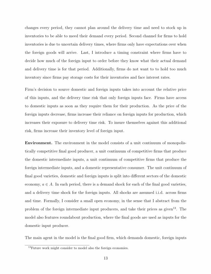
changes every period, they cannot plan around the delivery time and need to stock up in

inventories to be able to meed their demand every period. Second channel for firms to hold

inventories is due to uncertain delivery times, where firms only have expectations over when

the foreign goods will arrive. Last, I introduce a timing constraint where firms have to

decide how much of the foreign input to order before they know what their actual demand

and delivery time is for that period. Additionally, firms do not want to to hold too much

inventory since firms pay storage costs for their inventories and face interest rates.

Firm’s decision to source domestic and foreign inputs takes into account the relative price

of this inputs, and the delivery time risk that only foreign inputs face. Firms have access

to domestic inputs as soon as they require them for their production. As the price of the

foreign inputs decrease, firms increase their reliance on foreign inputs for production, which

increases their exposure to delivery time risk. To insure themselves against this additional

risk, firms increase their inventory level of foreign input.

Environment. The environment in the model consists of a unit continuum of monopolis-

tically competitive final good producer, a unit continuum of competitive firms that produce

the domestic intermediate inputs, a unit continuum of competitive firms that produce the

foreign intermediate inputs, and a domestic representative consumer. The unit continuum of

final good varieties, domestic and foreign inputs is split into different sectors of the domestic

economy, a ∈ A. In each period, there is a demand shock for each of the final good varieties,

and a delivery time shock for the foreign inputs. All shocks are assumed i.i.d. across firms

and time. Formally, I consider a small open economy, in the sense that I abstract from the

problem of the foreign intermediate input producers, and take their prices as given13. The

model also features roundabout production, where the final goods are used as inputs for the

domestic input producer.

The main agent in the model is the final good firm, which demands domestic, foreign inputs

13Future work might consider to model also the foreign economies.

13

and labor to produce a final good variety, and stores inventories of the final good firm.

Timing. One of the incentives for final good firms to hold inventories is given by the timing

constraint that is detailed below.

1. At the beginning of the period, the final good firms, j ∈ [0, 1], observe their level of

inventories, sj, and decide on the amount of the new order for foreign input, nj.

2. The final good firm specific demand and delivery time shock are realized, ηj = (νj, λj)

and a fraction λj of the new order of foreign input arrives and can be used for production

of this period.

3. Production and consumption take place.

4. At the end of the period the remaining fraction of the order, 1− λj, arrives.

Since final good firms need to put in the order of foreign inputs before the demand and

delivery time shocks are realized, they will place the order according to the expected value

of the shocks. On one hand, if firms have a realized low demand shocks and/or access to

a high portion of their new order, firms will need to store some of the foreign input as

inventory for the next period. Otherwise, if the realized demand shock is high, and/or firms

have access to a low proportion of their new order, then firms might be constrained in their

use of foreign inputs if they don’t have enough inventories in stock.

Final good producers. There is a unit continuum of domestic monopolistically competitive

final good producers, each producing a different variety j, of the final good, yj, which is

consumed by the domestic consumer. Each final good producer belongs to a specific sector

of the economy (within the unit continuum) j ∈ Ia.

The new order of foreign inputs, nj, face uncertain delivery times of arrival, where only a λj

fraction of the order is be available for consumption that period, and the remaining fraction,

1− λj, can be used for production until next period. Every period, the delivery time shock,

λj is drawn iid from a distribution G(λ). The amount of foreign inputs used in production,

14

xfj , is constrained by the level of inventories the firms has that period, sj, and the fraction

of the order the firms has access to that period, λjnj.

xfj ≤ sj + λj nj (1)

Final good firms take into account the demand of the domestic consumer for the final good,

and thus set prices. There is a per period, variety specific demand shock νj, which is

distributed log normal, with zero mean and variance σνa which varies across sectors, a. The

demand is given by the demand shock νj, the price of the final good, pj, set by the final

good firms, and the expenditure set for each variety of the final good.

yj(pj) = νj p−εj γa p

ε−1a P (C + N) (2)

νj ∼iid LogN( 0, σνa) (3)

The final good yj, j ∈ Ia is produced using domestic inputs, xdj , foreign inputs, xfj , and labor

lj. The production technology is Cobb-Douglas between the composite intermediate input

and labor; and a Constant Elasticity of Substitution (CES) aggregate with weights, θa, over

domestic and foreign inputs with elasticity of substitution σ. CES weights θa are sector

specific to reconcile the composition of foreign vs domestic use of inputs across different

manufacturing sectors in the economy. Additionally, I incorporate CES in the production

technology so the model is able to feature substitution of inputs used in production.

yj =(θ

1σ

a xd σ−1

σj + (1− θa)

1σ x

f σ−1σ

j

) σσ−1

α

` 1−αj (4)

Stock of inventories of foreign inputs, sj, face a storage cost δ. The law of motion for

inventories is given by the reminder of the inventories today that were not used to produce,

discounted at rate δ, and the (1−λj) fraction of the new order of foreign inputs nj that will

15

be available tomorrow.

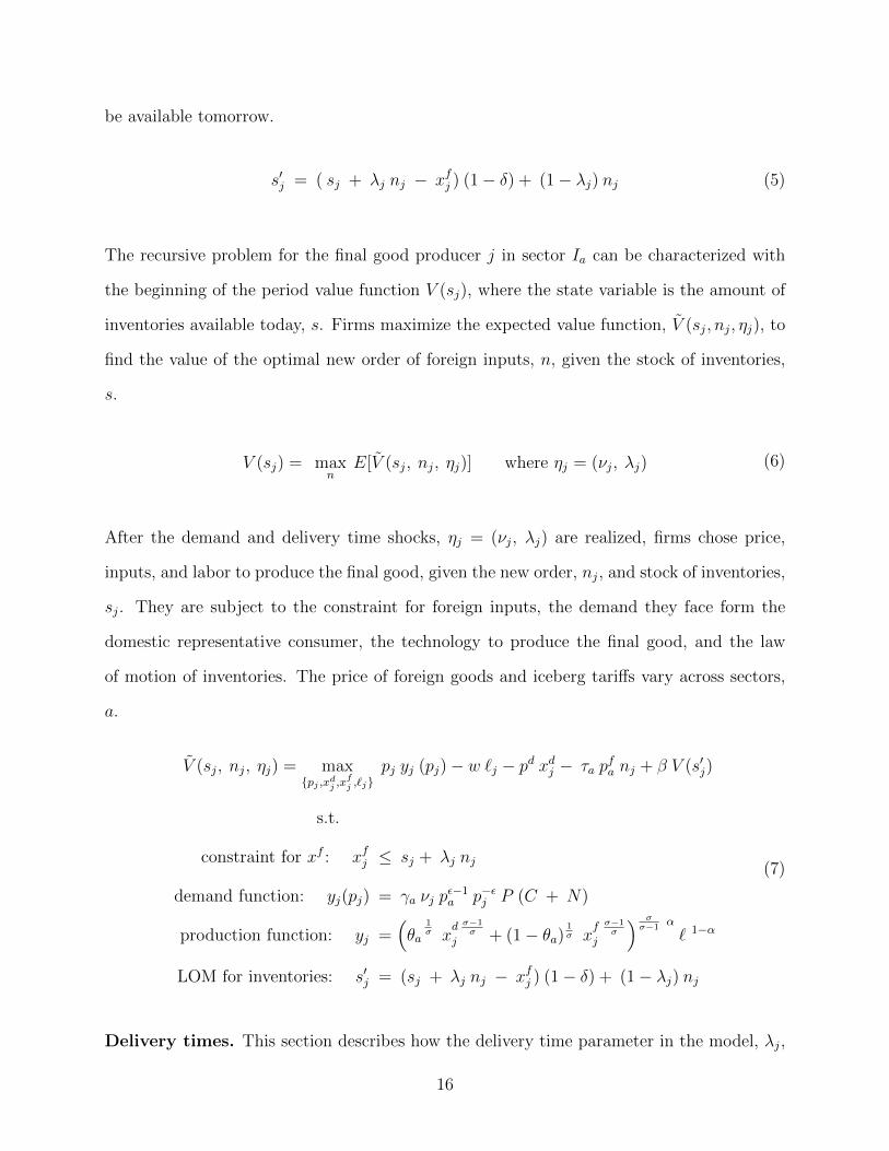
s′j = ( sj + λj nj − xfj ) (1− δ) + (1− λj) nj (5)

The recursive problem for the final good producer j in sector Ia can be characterized with

the beginning of the period value function V (sj), where the state variable is the amount of

inventories available today, s. Firms maximize the expected value function, V (sj, nj, ηj), to

find the value of the optimal new order of foreign inputs, n, given the stock of inventories,

s.

V (sj) = maxn

E[V (sj, nj, ηj)] where ηj = (νj, λj) (6)

After the demand and delivery time shocks, ηj = (νj, λj) are realized, firms chose price,

inputs, and labor to produce the final good, given the new order, nj, and stock of inventories,

sj. They are subject to the constraint for foreign inputs, the demand they face form the

domestic representative consumer, the technology to produce the final good, and the law

of motion of inventories. The price of foreign goods and iceberg tariffs vary across sectors,

a.

V (sj, nj, ηj) = max{pj ,xdj ,x

fj ,`j}

pj yj (pj)− w `j − pd xdj − τa pfa nj + β V (s′j)

s.t.

constraint for xf : xfj ≤ sj + λj nj

demand function: yj(pj) = γa νj pε−1a p−εj P (C + N)

production function: yj =(θ

1σ

a xd σ−1

σj + (1− θa)

1σ x

f σ−1σ

j

) σσ−1

α

` 1−α

LOM for inventories: s′j = (sj + λj nj − xfj ) (1− δ) + (1− λj) nj

(7)

Delivery times. This section describes how the delivery time parameter in the model, λj,

16

relates to the data. Assume each period represents a month, even though the specific value

of λj can be tailored to any period of time. In this case, λj represents the proportion of days

of the month (T = 30 days) the firm is able to use the order of foreign inputs to produce.

For example, assume a delivery time of 26 days, d = 26 days. The firms is able to use the

order for 4 (4 = 30 − 26) days of the month on average to produce. Then λj is related to

the delivery time days using:

λj = max( 0, 1− dj/T ) (8)

In this case λj = 4/30, which is the proportion of days a month the firms has the order

in the warehouse and is able to use it for production. Referring back to the law of motion

for inventories, equation 5, the storage costs are only paid for the proportion of the days

the goods were in the warehouse, λj. The goods in transit, (1 − λ)n, do not pay storage

costs.

Representative Consumer. The domestic representative consumer has preferences over

the final consumption good, C, and additionally sells the composite good N to domestic

intermediate inputs. They demand the unit continuum of final good varieties, yj. The unit

continuum is divided in different sectors, a = [1, ..., A] each with mass γa.

Each sectoral production, ya, is a CES aggregate with elasticity of substitution ε over the

final good varieties in sector a, yj, j ∈ Ia, where each final good variety is subject to a

demand shock, νj ∼iid LogN(0, σνa).

ya =

[∫j∈a

ν1εj y

ε−1ε

j dj

] εε−1

(9)

Then the sectoral production, is aggregated using a Cobb-Douglas function with weights γa

to obtain the final consumption good, C, and composite good, N . Roundabout production

is featured through the composite good, N , which aggregates the final good varieties and is

17

demanded by the domestic input producer to obtain intermediate inputs.

C + N =A∏a=1

yγaa whereA∑a=1

γa = 1 (10)

Domestic input producers. The unit continuum of competitive domestic intermediate

input producers, denoted by j ∈ [0, 1], use the composite good Ndj and labor ldj to produce

the input xdj using Cobb-Douglas technology.

xdj = N d αj ` d 1−αj (11)

Foreign input producers. There is a unit continuum j ∈ [0, 1] of competitive producers

of the foreign intermediate input, xfj . These goods face uncertain delivery times, λj and are

stored as inventories by the final good firms. I am abstracting from modeling this firms, but

rather taking as given the prices, pfa, and tariffs, τa, which vary across sectors.

Equilibrium. The general equilibrium steady state of this model is given by state contingent

policy functions for the final good firm, {nt(s), s′t(s), xdt (s, η), xft (s, η), `t(s, η)}∞t=0, for the

domestic input firms {Ndt , `

dt }∞t=0, and for the domestic consumer {yt, yat, Nt, Ct}∞t=0 and

prices {wt, pt, Pt, pat, pdt }∞t=0 such that the following conditions hold:

1. Policy functions solve the final good firm problem;

2. Policy functions solve the domestic input firm problem;

3. Policy functions solve the representative domestic consumer;

4. Price index for sectoral production prices, pa, and final consumption good and com-

posite good price, P , given by: pa =(∫

1

0νj p

1−εj

) 11−ε

and P = 1 /(∏

a(γa/pa)γa)

4. Final good market clears, where the demand by domestic consumer is equal to the

supply by the final good firm for each of the varieties, j ∈ [0, 1];

18

5. Domestic input market clears, where the demand by the final good firms is equal to

the supply by the domestic input firm for each of the varieties, j ∈ [0, 1];

6. Composite good market clears, where the supply given by the domestic consumer is

equal to the total demand by domestic input firms: N =∫

1

0Ndj dj

7. Labor market clears, where the fixed supply is equal to the labor demand by domestic

input firms and domestic final good firms: L =∫

1

0`dj dj +

∫1

0`j dj.

3.1 Policy Functions

This section describes the mechanism of the model through the main policy functions of

the final good firm. The graph 8a plots the policy function for the new orders of foreign

input, which depends on the level of inventories the firm begins the period with. New orders

decrease in the level of inventories, and remain at zero when inventories are high enough such

that they can cover the expected demand. The two vertical lines define where the stationary

distribution lies. Graph 8b plots the demand for foreign inputs for production for different

combination of shocks for demand and delivery time, for each value of inventories. Since the

orders are placed before shocks are known and inventories are costly, when firms have high

demand shocks and low access to a low proportion of the order (solid blue line), firms will be

constrained in the amount of foreign inputs they need to meet their unconstrained production

in the stationary distribution. On the other hand, when firms have a low demand shock and

access to a high proportion of the order (dashed red line), then the amount available of the

foreign good will be enough for them to meet their unconstrained production.

Graph 8d show how prices adjust upwards when firms are constrained (solid blue line). As

inventories increase, and firms are less constrained in the amount of foreign inputs they can

use in production, prices decrease until they reach their unconstrained optimal. The level of

inventories tomorrow is shown in graph 8c, given the specific shocks and level of inventories

19

the firm starts the period with. In the stationary distribution, when firms are constrained,

they use all the stock of inventories they have access to that period to produce, and the

inventories tomorrow will consist of the (1 − λ) fraction of the order that arrives until the

end of the period. If unconstrained (red dashed line), inventories tomorrow will consist of

whatever is left over from production today, and the (1−λ) fraction of the order that arrives

until the end of the period.

Figure 8: Policy functions of key variables

(a) New order of foreign input, n (b) Foreign inputs used in production, xf

(c) Inventory at the end of the period (d) Price of final goods

20

4 Calibration

To answer the questions of the paper, this section describes the initial calibration of the

model. I assume the domestic economy is the U.S. manufacturing industry and the foreign

input firms are settled in China. I calibrate the parameters of the model to match key

moments of the 2005 U.S. manufacturing economy. The summary of the values of the

parameters is reported in table 2.

I interpret the length of the period as one month, which is consistent with the delivery times

between the route from China to U.S. I begin by ranking the 17 NAICS 3-digit manufacturing

sectors according to their share of total imported inputs, and aggregate them into three

sectors, such that each represents one third of total gross output. In the model, the unit

continuum of final good varieties is split in the three sectors, each with equal mass. Sectoral

shares given by γa are equal to one third for all sectors.

The input share in the technology production functions for the domestic input and final

good firms, α, is obtained using data from the Input-Output tables from the BEA. The

input share is given by the value of intermediate inputs over total industry output, which

for the year 2005 equals 0.6314.

I set the discount factor, β, to 0.961/12 which corresponds to a 4% annual interest rate. To

obtain the value for the storage cost, δ, I refer to the inventory carrying cost literature and

set it to δ = 0.025, which implies a 30% annual storage cost15. The elasticity of substitution

between foreign and domestic inputs used in the production of the final good, σ, and the

elasticity over the final good varieties, ε, are set to 1.5. This value is the mean in the literature

for the manufacturing sector in the U.S. according to Bajzik et al. (2019). I modify this values

and detail the changes in the sensitivity section.

14The value of intermediate inputs over total gross output remains relatively constant across time andsectors. I fix α constant across manufacturing sectors and set it to the year 2005

15Carrying costs include storage costs, handling, administrative work, taxes, spoilage, etc. This annualinventory costs range from 19% to 43% according to Alessandria et al. (2010a)

21

The weights for the domestic inputs in the technology function for final good firms, are

calibrated inside the model to match the share of imported inputs observed in the data

across manufacturing sectors. To match the input inventory (work in process inventory)

over sales observed in the data across manufacturing sectors I calibrate the variance of

the demand shocks inside the model. Given the strategy used to create the sectors in the

model and the positive relationship between imported inputs and inventory level, the input

inventory over sales increases across sectors. The values for this parameters are shown in

table 2. The calibration of the delivery times is detailed in the subsection below.

4.1 Delivery times

To calibrate the delivery times of the model for U.S.-China trade I use data for the mean of

delivery days and the average length of delays. On average, 80% of the goods coming from

China are transported via ocean, and the remaining 20% arrive via air. Rough estimates of

delivery times are obtained from Freightos, an online freight shipping marketplace platform

thats specializes in the U.S.-China route.

Ocean transportation from China takes around 25 days to arrive to the West Coast, and

35 days to the East Coast. The variance associated to ocean vessel in this route is around

+/- 10 days16. For air transportation, the mean of delivery times is around 10 days, with a

possible early or late arrival of 3 days.

To obtain the distribution of delivery days from China, d ∼ g(µd, σd) I assume a bimodal

distribution of two lognormal probability distributions, where the mixing parameter equals

to 0.8 for the ocean distribution, and 0.2 for the air distribution.

g(d) = 0.8 gocean(d) + 0.2 gair(d) (12)

16A new dataset property of Tom Holmes will allow me to obtain more details on the delivery times anddelays to inform the parameters of the model.

22

To obtain the mean and standard deviation of the lognormal distributions for air and ocean

transportation, I assume the geometric mean of the distribution, µd, is equal to mean of

delivery time, and I compute the standard deviation such that around 95% of the distribution

lies within the observed variance in the data. Using this methodology, for China’s ocean and

air transportation, docean ∼ LogN(30, 1.7), and dair ∼ LogN(10, 0.5).

Finally, to obtain the distribution for λ I use equation 8, λ = max( 0, 1 − d/30), which

assumes that a period of time is a month, and apply a linear transformation to the bimodal

distribution of delivery days, g(d).

Table 2: Benchmark Calibration

Outside the modelParameter Value Comment

Number of sectors 3 Rank the share of imported inputs, and combinethe 17 NAICS-3 to 3 sectors

Sector share γa 1/3 Gross output share of each sector in 2005Input share α 0.63 I-O tables: α2005 = intermediate input/outputDelivery times λ g(d) = 0.8goc + 0.2gair

docean ∼ LogN(30, 1.7)dair ∼ LogN(10, 0.5)

PredeterminedParameter Value Comment

Elasticity of sub. xf , xd σ 1.5 Bajzik, Kavranek, Irsova and Schwarz 2019Elasticity of sub. yj ε 1.5 Bajzik, Kavranek, Irsova and Schwarz 2019Monthly interest rate β 0.961/12 4% annual interest rateMonthly storage rate δ 0.025 30% annual rate

Inside the modelParameter Value Moment Model Data (2005)

Weight dom. inputs 1 θ1 89.7% share imported inputs 1 10.2% 10.3%Weight dom. inputs 2 θ2 85.1% share imported inputs 2 14.7% 14.9%Weight dom. inputs 3 θ3 78.8% share imported inputs 3 21.0% 21.2%Variance of demand 1 σν1 0.619 input inventory/GO 1 21.3% 21.5%Variance of demand 2 σν2 0.570 input inventory/GO 2 27.3% 26.9%Variance of demand 3 σν3 0.708 input inventory/GO 3 53.8% 53.7%

23

5 Quantitative Results

This section describes the methodology and results for the research questions of the pa-

per.

5.1 Inventories as insurance of delivery time risk

When firms decide to incorporate foreign intermediate inputs to their production process,

they have to take into account the delivery time risk associated to these cheaper inputs. To

measure the delivery time risk these inputs face, I compare two general equilibrium steady

states with different shares of imported inputs. I start with the calibrated initial steady state

and compare it to a steady state where I match the observed share of imported inputs from

2018. For the 2018 steady state I use the initial value of the parameters (calibrated to U.S.

2005 manufacturing ) and calibrate the price of the foreign inputs to match the 2018 share

of imported inputs across sectors. The results are summarized in 3 and 4.

To understand how much added delivery time risk is associated to the increase in the share

of imported inputs from China, I look at the change in inventories as a share of gross output,

(st+1− st)/yt. I observe that for sector two, an increase in 1.9 percentage points in the share

of imported inputs is related to an inventories increase of 5.4% of gross output. The cost

of the inventory increase, defined as δ(st+1 − st)/yt, is of 1.6%. The cost of insurance is

significant when compared to the 1.3% increase in gross output for sector two, and the 1.1%

increase in total consumption. Similar results are obtain for the three manufacturing sectors

in table 4. This results highlight the importance of taking into account the cost of delivery

time risk when studying global supply chains and the benefits from trade. Additionally it

provides a measure of the magnitude of delivery time risk that firms are willing to insure

away via inventories.

The price of foreign inputs of sector two decreases 10.5% to match the 1.9 percentage point

24

increase in imported input in the data. The foreign price decrease results in an increase

in consumption, and gross output across sectors. The decrease in domestic prices is less

than the change in foreign input price due to the general equilibrium effects, where there is

a demand increase for the domestic inputs. The roundabout production enables a channel

for the decrease in the price of the foreign goods to be fed back into the domestic input

producers, where the demand for composite input increases 0.6%.

Table 3: Import share for 2018

Price foreign input Change Moment Model Data 2018 Data 2005

sector 1: pf1 −1.4% share imported inputs 1 10.6% 10.7% 10.3%

sector 2: pf2 −10.5% share imported inputs 2 16.8% 16.8% 14.9%

sector 3: pf3 −6.8% share imported inputs 3 22.6% 22.6% 21.2%

Table 4: Steady state model results: comparison

Variable Initial 2005 Final 2018

Consumption C 1.1% increaseComposite good N 0.6% increaseGross output (avg) y1 0.5% increase

y2 1.5% increasey3 1.3% increase

Final price index P 1.1% decreaseSectoral output price p1 0.5% decrease

p2 1.5% decreasep3 1.3% decrease

Domestic input price pd 0.7% decreaseInput inventory over gross output (avg) s1/y1 21.5% 22.3%

s2/y2 26.9% 31.9%s3/y3 53.7% 58.3%

Input inventory change (avg) (∆s1)/y1 0.9% increase(∆s2)/y2 5.4% increase(∆s3)/y3 5.4% increase

Cost of insurance δ(∆s1)/y1 0.3%δ(∆s2)/y2 1.6%δ(∆s3)/y3 1.6%

25

5.2 Rise in inventories and insurance needs from inputs from

China

U.S. manufacturing inventories have been increasing since 2005, and there are many reasons

why inventories would have increased in this period. This paper focuses on the channel of

delivery time risk of inputs, and in this section I use the model to estimate how much of

the increase in inventories can be explained by insurance needs from sourcing inputs from

China.

To do so, I compute partial equilibrium transition paths for the period 2006 to 2018. The

initial calibration of 2005 U.S. manufacturing industry matches the total share of imported

inputs across sectors, and in this section I match the increase of imported inputs that is

coming from China for the period 2006 to 2018. I begin by computing the final steady state

using the parameters from the initial calibration to 2005 U.S. manufacturing industry, and

match the share of the increase in imported inputs from China in 2018 using the price of

foreign inputs17. Then using backward induction, I obtain the stationary distributions of

every period where I match the import share from China with the price of foreign input for

each sector.

Figure 9 shows the import share across sectors for the model and data, where they match

perfectly to obtain the implied foreign price index for each sector. Then using the foreign

input prices I obtain the average inventory over gross output in each period for each sector,

shown in figure 10. For some sectors and periods more than others, but the model is able

to replicate some of the increase in input inventories in the data for the period of 2006 to

2018. The increase in inventories is coming from the increase in reliance on foreign inputs

and due to the insurance needs against the additional delivery time risk.

On average, 47% of the increase in U.S. manufacturing inventories for 2006 - 2018 can be

17I start with the total share of imported inputs in 2005 and then feed the increase in imported inputsthat is coming from China.

26

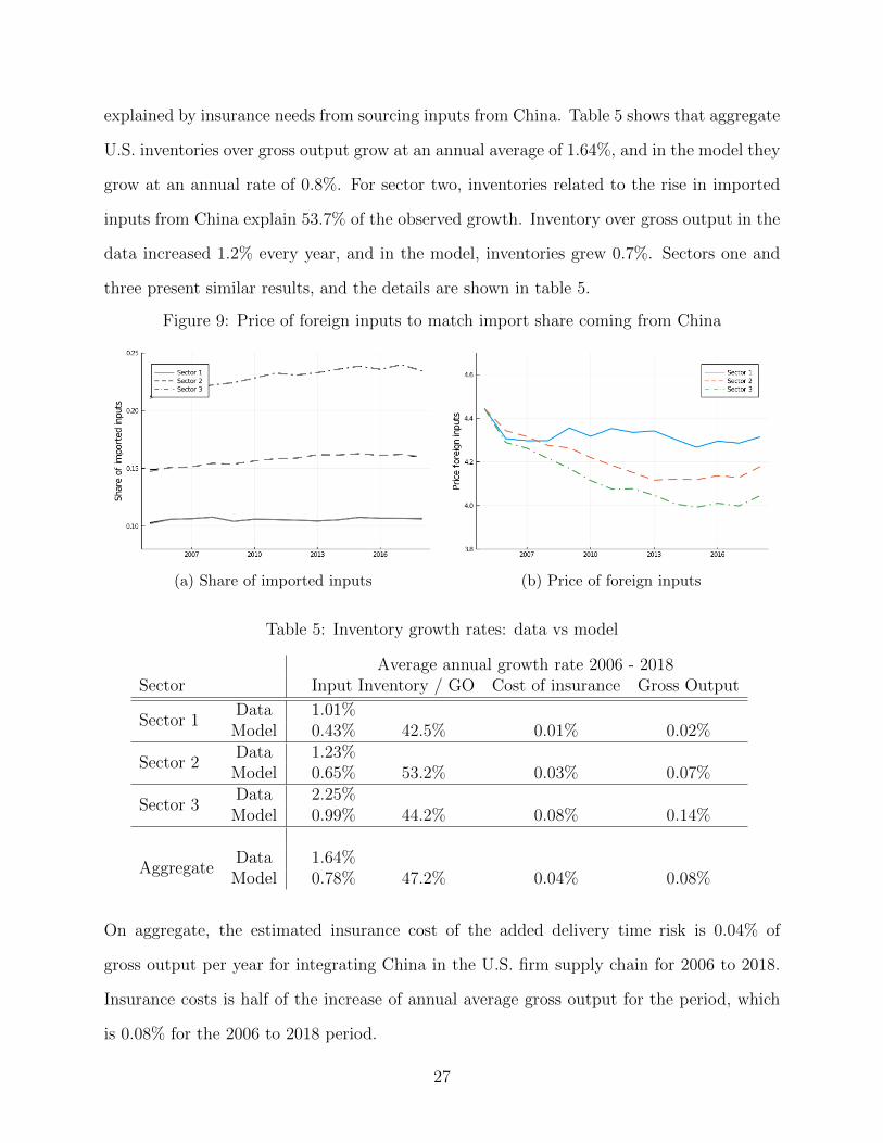
explained by insurance needs from sourcing inputs from China. Table 5 shows that aggregate

U.S. inventories over gross output grow at an annual average of 1.64%, and in the model they

grow at an annual rate of 0.8%. For sector two, inventories related to the rise in imported

inputs from China explain 53.7% of the observed growth. Inventory over gross output in the

data increased 1.2% every year, and in the model, inventories grew 0.7%. Sectors one and

three present similar results, and the details are shown in table 5.

Figure 9: Price of foreign inputs to match import share coming from China

(a) Share of imported inputs (b) Price of foreign inputs

Table 5: Inventory growth rates: data vs model

Average annual growth rate 2006 - 2018Sector Input Inventory / GO Cost of insurance Gross Output

Sector 1Data 1.01%

Model 0.43% 42.5% 0.01% 0.02%

Sector 2Data 1.23%

Model 0.65% 53.2% 0.03% 0.07%

Sector 3Data 2.25%

Model 0.99% 44.2% 0.08% 0.14%

AggregateData 1.64%

Model 0.78% 47.2% 0.04% 0.08%

On aggregate, the estimated insurance cost of the added delivery time risk is 0.04% of

gross output per year for integrating China in the U.S. firm supply chain for 2006 to 2018.

Insurance costs is half of the increase of annual average gross output for the period, which

is 0.08% for the 2006 to 2018 period.

27

Figure 10: Inventory over gross output

(a) Sector 1 (b) Sector 2

(c) Sector 3

6 Sensitivity (to do)

1. Different values of σ, ε, β, δ

• Include data analysis of elasticity of substitution

2. Robustness check for mean and variance of delivery times, λ

3. Calibrate quarterly model

4. Decomposition of different incentives for inventories:

(a) Eliminate timing constraint

(b) No delays: σλ = 0

28

(c) No mean of delivery times (but keep delays): µλ = 0 and σλ > 0

(d) Only timing constraint - no delivery time risk: µλ = 0 and σλ = 0

7 Conclusion

References

David Hummels and Georg Schaur. Time as a trade barrier. American Economic Review,

2013.

George Alessandria, Joseph P. Kaboski, and Virgiliu Midrigan. Inventories, lumpy trade,

and large devaluations. American Economic Review, 2010a.

Ana Filipa Vieira Nadais. Essays on international trade and international macroeconomics.

Thesis, 2017.

Shafaat Y. Khan and Armen Khederlarian. Inventories, input costs and productivity gains

from trade liberalizations. Working Paper, 2020a.

George Alessandria, Joseph P. Kaboski, and Virgiliu Midrigan. Trade wedges, inventories,

and international business cycles. Working Paper, 2010b.

George Alessandria, Joseph P. Kaboski, and Virgiliu Midrigan. The great trade collapse of

2008-09: An inventory adjustment? IMF Economic Review, 2010c.

David Hummels. Transportation costs and international trade in the second era of global-

ization. Journal of Economic Perspectives, 2007.

Sebastian Heise, Justin Pierce, Georg Schaur, and Peter Schott. Trade policy uncertainty

and the structure of supply chains. Working Paper, 2019.

29

George Alessandria, Shafaat Y. Khan, and Armen Khederrlarian. Taking sock of trade policy

uncertainty: Evidence from china’s pre-wto accession. Work in Process, 2020.

Shafaat Y. Khan and Armen Khederlarian. How does trade respond to anticipated tariff

changes? evidence from nafta. Working Paper, 2020b.

Peter K. Schott. The relative sophisitication of chinese exports. Economic Policy, 2008.

Jhon T. Dalton. A theory of just-in-time and the growth in manufacturing trade. Work in

Process, 2013.

Josef Bajzik, Tomas Havranek, Zuzana Irsova, and Jiri Sxhwarz. The elasticity of substitu-

tion between domestic and foreign goods: A quantitative survey. ECONSTOR, 2019.

A Solving the Model

I assume I know the model parameters {β, ε, α, σ, δ, L, (γa, θa, σνa , τa, µλa , σλa)∀a, }. Then I

follow the structure detailed below.

1. I start with an initial guess for the composite good and sectoral output prices, (N, (pa)∀a),

and I normalize the wage to one, w = 1.

2. Given the values for (N, (pa)∀a, w = 1), I find the aggregate variables, (C, (ya)∀a) and

prices (P, pd) according to the equations below.

1

P=∏a

(γapa

)γa

C =w L

P

ya =γa P (C +N)

pa

pd =P α w 1−α

α α (1− α) 1−α

30

3. Given the aggregate variables, (C,N, (ya)∀a), and prices (P, pd, w, (pa)∀a), I solve for

the problem of the final good firms. I obtain the policy function for the new orders

and value function, (n(s), V (s) for a given inventory level, s. Additionally I solve for

the policy functions for (n, s′, xf , xd, `, p) for a given inventory level, s, and specific

combination of demand and delivery time shock, η = (ν, λ).

V (s) = maxn

E[V (n)(s, η)] where η = (ν, λ)

V (n)(s, η) = max{p,xd,xf ,`}

p y (p)− w `− pd xd − τa pfa n+ β V (s′)

(a) First step is to obtain the policy functions of (s′, xf , xd, `, p) for values of (s, n, η).

I create a grid for the state variables (s, η). The policy function (p, xd, xf , x, `, s′)

will be a function of n and defined for each (s, η)

i. Solve for the unconstrained equilibrium, using the first order conditions of

the final good firm problem:

1

pj=

ε− 1

ε

αα (1− α)1−α

w1−α

(θa

pd σ−1+ (1− θa)

(1− δλj1− δ

1

τa pfa

)σ−1) ασ−1

yj = pεa p−εj ya νj

xj =ε− 1

εα pj yj

(θa

pd σ−1+ (1− θa)

(1− δλj1− δ

1

τa pfa

)σ−1) 1σ−1

xfj =(ε− 1

εα pj yj

)σ (1− δλj1− δ

)σ 1− θaxσ−1j (τa p

fa)σ

xdj =(ε− 1

εα pj yj

)σ θa

xσ−1j pd σ

` =ε− 1

ε(1− α)

pj yjw

s′j = (sj + λjnj − xfj ) (1− δ) + (1− λj) nj

ii. Solve for the constrained equilibrium, using the first order conditions of the

31

final good firm problem:

xfj = sj + λj nj

yj = xαj `1−αj

pj = pa

(yaνj yj

) 1ε

xj =

(θ

1θaa x

d σ−1σ

j + (1− θa)1θa x

f σ−1σ

j

) σσ−1

xdj =(ε− 1

εα pj yj

)σ θa

xσ−1j pd σ

`j =ε− 1

ε(1− α)

pj yjw

s′j = (sj + λjnj − xfj ) (1− δ) + (1− λj) nj

iii. If the unconstrained demand of foreign input satisfies xfunc < s+λn, then the

value in the policy function is the unconstrained values , and otherwise I use

the constrained values to solve for the policy function.

(b) I start with a guess for the value function V (s′), and use the policy function to

calculate the value function V (n)(s, η) (function of n, for each value of (s, η)).

V (n)(s, η) = max{p,xd,xf ,`}

p y (p)− w `− pd xd − τa pfa n+ β V (s′)

(c) Given the value function V (n)(s, η), I obtain the expected value assuming iid

distribution for η, Eη[V (n)(s, η)], and optimize to obtain the policy function of

n for each value of s in the grid.

(d) With the values of the policy function for each value of inventories s, I use value

32

function iteration to obtain the value function V (s) of the final good firm.

V (s) = Eη

[p∗ y (p∗)− w `∗ − pd xd∗ − τa p

f∗a n∗ + β V (s

′∗)]

4. Using the policy functions of (pj, xdj ), I obtain the demand functions of the domestic

input firm for the composite good, Ndj , and labor demand `dj .

`dj =(1− α) pj x

dj

w

Ndj =

(α) pj xdj

P

5. I solve for the stationary distribution by fixing the exogenous random process of η,

and then use Monte Carlo where I solve for 100, 000 firms for 200 periods (making sure

distributions converge).

6. Finally I update the composite aggregate, N , and the sectoral prices, (pa)∀a. Note the

wage is normalized so I drop the labor market clearing equation, according to Walras

Law. I run a loop to find the fixed point of this variables.

pa =

(∫Ia

νj p1−εj dj

) 11−ε

∀a

N =

∫ 1

0

Ndj dj

33