A

tppfaaudrt©

K

1

tce

w

r

0

Available online at www.sciencedirect.com

ScienceDirect

Computer Speech and Language 28 (2014) 709–726

Incorporating local information of the acoustic environments toMAP-based feature compensation and acoustic model

adaptation�,��

Yu Tsao a,∗, Xugang Lu b, Paul Dixon b, Ting-yao Hu a, Shigeki Matsuda b, Chiori Hori b

a Research Center for Information Technology Innovation, Academia Sinica, No. 128, Academia Road, Section 2, Nankang, Taipei 11529, Taiwanb National Institute of Information and Communications Technology, (NICT), 3-5 Hikaridai, Keihanna Science City 6190289, Japan

Received 27 May 2013; received in revised form 20 November 2013; accepted 21 November 2013Available online 4 December 2013

bstract

The maximum a posteriori (MAP) criterion is popularly used for feature compensation (FC) and acoustic model adaptation (MA)o reduce the mismatch between training and testing data sets. MAP-based FC and MA require prior densities of mapping functionarameters, and designing suitable prior densities plays an important role in obtaining satisfactory performance. In this paper, weropose to use an environment structuring framework to provide suitable prior densities for facilitating MAP-based FC and MAor robust speech recognition. The framework is constructed in a two-stage hierarchical tree structure using environment clusteringnd partitioning processes. The constructed framework is highly capable of characterizing local information about complex speakernd speaking acoustic conditions. The local information is utilized to specify hyper-parameters in prior densities, which are thensed in MAP-based FC and MA to handle the mismatch issue. We evaluated the proposed framework on Aurora-2, a connectedigit recognition task, and Aurora-4, a large vocabulary continuous speech recognition (LVCSR) task. On both tasks, experimentalesults showed that with the prepared environment structuring framework, we could obtain suitable prior densities for enhancinghe performance of MAP-based FC and MA.

2013 The Authors. Published by Elsevier Ltd. All rights reserved.

eywords: MAP; Feature compensation; Acoustic model adaptation; Local information; Hyper-parameter specification; Noise robustness

. Introduction

Applications of automatic speech recognition (ASR) have received considerable attention in recent years. However,

he applicability of ASR is seriously limited by the fact that its performance can deteriorate when training and testingonditions do not match (Acero, 1990; Gong, 1995; Junqua et al., 1996; Huo and Lee, 2000; Huang et al., 2001; Molaut al., 2003; Deng and Huang, 2004). Maintaining satisfactorily robust performance under mismatched conditions is

� This is an open-access article distributed under the terms of the Creative Commons Attribution-NonCommercial-No Derivative Works License,hich permits non-commercial use, distribution, and reproduction in any medium, provided the original author and source are credited.

�� This paper has been recommended for acceptance by Prof. K. Shinoda.∗ Corresponding author. Tel.: +886 2 2787 2300/2390; fax: +886 2 2787 2315.

E-mail addresses: yu.tsao@citi.sinica.edu.tw (Y. Tsao), xugang.lu@nict.go.jp (X. Lu), paul.dixon@nict.go.jp (P. Dixon),99942144@ntu.edu.tw (T.-y. Hu), shigeki.matsuda@nict.go.jp (S. Matsuda), chiori.hori@nict.go.jp (C. Hori).

885-2308/$ – see front matter © 2013 The Authors. Published by Elsevier Ltd. All rights reserved.http://dx.doi.org/10.1016/j.csl.2013.11.005

710 Y. Tsao et al. / Computer Speech and Language 28 (2014) 709–726

an essential task for ASR applications. Handling the mismatch is difficult, because it generally comes from multiplesources, including inter- and intra-speaker effects, additive noise, convolutive transmission, and channel distortions.The overall effect of these distortions can be complex and hard to characterize. Many robustness approaches have beenproposed to handle the mismatch issue. These approaches can be categorized into three groups, signal-space, feature-space, and model-space approaches (Sankar and Lee, 1996; Lee, 1998), based on the space in which the mismatchissue is handled.

The signal-space approach (also known as speech enhancement methods) aims to reduce noise components fromnoisy speech signals while avoiding large speech distortions. Classical algorithms include spectral subtraction (SS)(Boll, 1979), Wiener filtering techniques (Scalart and Filho, 1996; Hansler and Schmidt, 2006; Chen et al., 2007),minimum mean square error spectral estimator (MMSE) (Ephraim and Malah, 1984; Martin, 2005; Hansen et al., 2006),minimum mean-square error log-spectral amplitude estimator (LSA) (Ephraim and Malah, 1985), maximum a posteriorispectral amplitude estimator (MAPA) (Lotter and Vary, 2005), and maximum likelihood spectral amplitude estimator(MLSA) (Kjems and Jensen, 2012). In the meanwhile, some models that characterize human speech production systemswere often incorporated for speech enhancement, such as harmonic model (Quatieri and McAulay, 1992), the linearprediction (LP) model (Makhoul, 1976), and the hidden Markov model (HMM) (Ephraim, 1992).

The feature-space approach tries to generate feature vectors that are robust to environment mismatches. Theseapproaches can be divided into two categories, feature processing (FP) and feature compensation (FC). FP methodsprocess both training and testing data sets to remove mismatches on features. Temporal filtering and feature normaliza-tion methods are two effective classes of FP approaches. Representative temporal filtering algorithms include relativespectral (RASTA) (Hermansky and Morgan, 1994), moving average and auto-regression moving average (Chen et al.,2002a, 2002b), which try to smooth acoustic features to suppress noise interferences. Feature normalization methodsaim to reduce the mismatch by mapping training and testing acoustic features to make them close to each other in thefirst or higher order statistical measures. Successful algorithms include cepstral mean subtraction (CMS) (Viikki andLaurila, 1998; Kim and Rose, 2003), cepstral mean and variance normalization (CMVN) (Tibrewala and Hermansky,1997), and histogram equalization (HEQ) (Ibm et al., 2000). On the other hand, FC methods compute a mapping func-tion to characterize the environmental mismatch. The acoustic features are then transformed by the mapping functionto match the acoustic model. A variety of mapping functions has been applied in previous studies, among which affinetransform and compensation bias are two popular choices. Notable examples include maximum likelihood (ML) andmaximum a posteriori (MAP) based stochastic feature matching (SFM) (Lee, 1998; Jiang et al., 2001), feature spacemaximum likelihood linear regression (feature space MLLR (Gales, 1997)) and maximum a posteriori linear regression(feature space MAPLR (Li et al., 2002)).

The goal of the model-space approach is to estimate an acoustic model that is more robust to environmental changesor matches the testing condition better. Two classes of model-space approaches, discriminative training (DT) andmodel adaptation (MA), have been confirmed to be effective and are widely used. Generally, DT approaches usean objective function that measures the separation between parameters in a set of acoustic models. The objectivefunction is optimized based on training data to increase the separation between model parameters. Well-known DTapproaches include minimum classification error (MCE) (Juang et al., 1997), maximum mutual information estimation(MMIE) (Valtchev et al., 1997), minimum phone error (MPE) (Povey and Woodland, 2002), large margin estimation(LME) (Jiang et al., 2006), and soft margin estimation (SME) (Li et al., 2007) methods. On the other hand, MAapproaches estimate a mapping function to adjust parameters in the original acoustic model to match the testingcondition. Successful examples include stochastic matching algorithm (Sankar and Lee, 1996; Lee, 1998), maximuma posteriori (MAP) (Gauvain and Lee, 1994; Huo et al., 1995), MLLR (Leggetter and Woodland, 1995; Gales, 1997),and MAPLR (Chesta et al., 1999; Siohan et al., 2001).

In the reviewed approaches above, MAP-based FC and MA estimate mapping functions based on the MAP criterionto compensate for acoustic mismatches. Owing to their efficiency and flexibility, they have received extensive attentionin recent years (Gauvain and Lee, 1994; Chesta et al., 1999; Siohan et al., 2001; Jiang et al., 2001; Li et al., 2002).These approaches require prior densities of the mapping function parameters, and determining suitable densities is animportant task in obtaining satisfactory performance. Traditionally, prior densities were designed without considering

the underlying environment structures, so the prior density could not characterize the local statistical structure of theacoustic environments. In this paper, we propose an environment structuring framework for exploring local informationof the ensemble speaker and speaking environment conditions. Based on local information, we derive suitable priordensities for MAP-based FC and MA. We conducted experiments using two standardized speech databases, Aurora-2

Y. Tsao et al. / Computer Speech and Language 28 (2014) 709–726 711

(2M

edr

2

e

2

F

wc

wfM

a

we

Fig. 1. FC and MA processes in ASR.

Pearce and Hirsch, 2000; Macho et al., 2002) and Aurora-4 (Hirsch, 2001; Parihar and Picone, 2002; Parihar et al.,004). Experimental results confirmed the effectiveness of our proposed idea for enhancing the MAP-based FC andA capability to handle the mismatch issue.The reminder of this paper is organized as follows. Section 2 reviews MAP-based FC and MA and introduces the

nvironment structuring framework. Section 3 describes four algorithms for specifying hyper-parameters of the priorensities based on the environment structuring framework. Section 4 shows our experimental setup and evaluationesults. Section 5 concludes the study by summarizing our findings.

. Feature compensation and model adaptation with an environment structuring framework

This section first reviews the fundamental theories of MAP-based FC and MA. Then we introduce the proposednvironment structuring framework used for prior density specification.

.1. MAP-based FC and MA

Fig. 1 illustrates FC and MA in a speech recognition system. FC transforms the original testing speech features,Y, to new speech features, FX, that match the acoustic model for the training condition by

FX = Γυ(FY) (1)

here Γ υ(.) is an FC mapping function, and υ denotes the parameters in the FC mapping function. We use the MAPriterion to calculate υ in Γ υ(.) by

υ̂ = argmaxυP(FY|υ, ΛX)[(p(υ)]�, (2)

here � is a forgetting factor, p(υ) is the prior density for FC (Jiang et al., 2001), and ΛX denotes the acoustic modelor the training condition. When setting � = 0 in Eq. (2), the estimation of υ̂ is exactly the same as that based on the

L criterion (Lee, 1998).In MA, a mapping function, Γ θ(.), is used to adjust parameters of the acoustic model for the training condition, ΛX,

nd generate a new acoustic model, ΛY, for the testing condition according to

ΛY = Γθ(ΛX), (3)

here Γ θ(.) characterizes the mismatch between the training and testing conditions. Similar to MAP-based FC, thestimation of the parameters, θ, in Γ θ(.), is formulated as

θ̂ = argmaxθ P(FY|θ, ΛX)[p(θ)]τ, (4)

712 Y. Tsao et al. / Computer Speech and Language 28 (2014) 709–726

Root

Layer lEC

Layer LEC

c-th EP Tre e

1-st EP Tre e

EC Tre e C-th EP Tre e

Fig. 2. Environment clustering and partitioning framework.

where τ is a forgetting factor, and p(θ) is the prior density for MA. We can also obtain the ML-based solution of θ̂ bysetting τ = 0 in Eq. (4).

In Eqs. (2) and (4), the hyper-parameters for the prior densities must be properly specified to characterize thestatistics of the underlying acoustic environments. In what follows, we introduce the proposed environment structuringframework for doing this.

2.2. Environment structuring framework

Two steps are involved in constructing the environment structuring framework, environment clustering (EC) andenvironment partitioning (EP) (Tsao and Lee, 2009). After these two steps, the environment structuring framework isstructured as a two-stage hierarchical tree, as shown in Fig. 2. The algorithms involved in these two steps are brieflyintroduced in the following discussion.

2.2.1. Environment clustering (EC)The goal of EC is to cluster the entire set of training data into several subsets. Each subset includes speech data

representing similar acoustic characteristics. As shown in Fig. 2, a hierarchical tree structure is adopted to perform EC.Assuming that the tree built using EC (named EC tree hereafter) has C nodes, including the root node, intermediatenodes, and leaf nodes, we accordingly cluster the entire set of training data into C subsets {Q1, Q2, . . ., QC}, whereeach subset contains local information about the entire set of training data. Next, we use the data in each subset toestimate an acoustic model and obtain C sets of acoustic models, {Λ1, Λ2, . . ., ΛC}. We use these C sets of acousticmodels to characterize local information about the entire acoustic space.

Some previous studies also proposed to structure the training data to facilitate the model adaptation process. In Zhanget al. (2003), training data is divided into several noisy clusters, which are used to prepare multiple HMM sets. Then anoisy cluster that best matches the testing utterance is located, and its corresponding HMM set is used for recognition.Additionally, an MLLR transformation is applied to further adapt the Gaussian mean parameters. In Padmanabhanet al. (1998), speaker clustering is first performed, and model adaptation is conducted based on linear transforamtionscaclulated by the cluster of speakers that is acoustically close to the testing speaker. The EC algorithm shares the similarconcept of the above appraoches, while we investigate to apply the constructed EC tree to not only model adapationbut also feature compensation. Furthermore, since the EC tree can characterize local informtion of the entire trainingacoustic space, we propose to utilize the local infromation to specify suitable prior densities for MAP-based FC andMA mapping fucntion estaimtions. These two parts will be dicsussed in more details in the following discussion.

2.2.2. Environment partitioning (EP)In Gales (1996), an acoustic space clustering and selection algorithm based on a regression tree was proposed. The

regression tree can be constructed based on the phonetic knowledge or in a data driven manner and was adopted to

Y. Tsao et al. / Computer Speech and Language 28 (2014) 709–726 713

1

2 3 4

EP Tree

Roo t

Layer lEP

Layer LEP

n-2n-1 n

r

{ Z1 ; 1 }

{ Z4 ; 4 }

{ Zr ; r }

{ Zn ; n }

fbacFdaaCi(tmZo

lmFcasa

2

p

wdaa

Fig. 3. Environment partitioning (EP) tree.

acilitate MLLR acoustic model adaptation. In Shinoda and Lee (2001), a hierarchical tree structure was used for MAPased model adaptation. Both approaches used the tree-structured clustering and selection methods for acoustic modeldaptation (Gales, 1996; Shinoda and Lee, 2001). The EP algorithm adopts the same idea to partition the Gaussianomponents in an acoustic model into several groups. Based on the EP algorithm, we build an EP tree, as shown inig. 3, which is used for both FC and MA. Moreover, based on the EP tree structure, we further design four priorensities to be used for MAP-based FC and MA (refer Section 3). In this study, we propose a two-stage tree structure,s shown in Fig. 2. For each of the C sets of acoustic models, {Λ1, Λ2, . . ., ΛC}, we estimate a tree using the EPlgorithm (named EP tree hereafter). Accordingly, we prepare C EP trees, {Ω1, Ω2, . . ., ΩC}, corresponding to the

acoustic models. The EP tree presented in Fig. 3 corresponds to one EP tree in Fig. 2. Assume that this EP treencludes N nodes, the entire set of Gaussian components in an acoustic model is accordingly partitioned into N groupsZ1, Z2, . . ., Zn, . . ., ZN), where Zn denotes the nth group of Gaussian components in the EP tree. Because each node inhe EP tree is obtained from separating the Gaussian components from its parent node, the Gaussian components are

utually exclusive in the nodes of the same layer and represent different acoustic properties. For the EP tree in Fig. 3,1 denotes the entire set of mean parameters, Φ1 represents the hyper-parameter set for Z1, Zn denotes the nth subsetf the entire set of mean vectors, and Φn represents the hyper-parameter set for Zn.

In the constructed environment structuring framework in Fig. 2, we have multiple acoustic models for characterizingocal acoustic conditions. These multiple acoustic models are used online to perform cluster selection (CS) for deter-

ining one acoustic condition that best matches the testing condition. The selected acoustic model is used to performC or/and MA, and the compensated features or/and adapted acoustic models are then used to test recognition. In theompensation or/and adaptation stage, the EP tree structure in Figs. 2 and 3 are used to specify prior densities, whichre used in MAP-based FC and MA. In our study, MAP-based stochastic feature matching (SFM) using a compen-ation bias is adopted for FC, and linear regression (LR) is chosen for MA. In the following, we introduce these twopproaches under the proposed environment structuring framework.

.3. MAP-based SFM

In Eq. (1), by setting FX = [f X1 f X

2 , . . ., f XT ] and FY = [f Y

1 f Y2 , . . ., f Y

T ], we perform a frame-wise feature com-ensation by

f Xt = Γυ(f Y

t ), t = 1, 2, . . ., T, (5)

here f Yt and f X

t are noisy and compensated features at the tth time index, respectively. To perform Eq. (5), we first

efine the form of the FC mapping function, Γ υ(.). Generally, when sufficient samples from the testing condition arevailable, a complex parametric function of Γ υ(.) can be used to compensate noise components accurately. When only

small number of samples is available, a simple form of Γ υ(.) should be used to avoid over-fitting. In this study, we

714 Y. Tsao et al. / Computer Speech and Language 28 (2014) 709–726

focus on the condition that only few data samples are available to estimate the compensation function. Therefore, weuse a simple compensation bias for Γ υ(.). Thus, Eq. (5) becomes

f Xt = f Y

t − δn, t = 1, 2, . . ., T, (6)

where δn is a compensation bias belonging to the nth node in the EP tree. To perform Eq. (6), we first decode FY

to generate a transcription reference. Then based on the transcription reference, we can obtain the node sequencecorresponding to FY = [f Y

1 f Y2 , . . ., f Y

T ] to perform SFM. Please note that the N biases, δn (n = 1, . . ., N), are sharedand used to compensate all of the testing feature vectors. Namely, the compensation is performed in a frame-wisemanner. Each particular feature vector, f Y

t , selects a particular bias δn to perform SFM, and the selection of n out ofN nodes is done by a searching process through the EP tree.

When applying MAP-based SFM to calculate δn, we first specify a prior density:

p(δn) ∝D∏

i=1

exp

[− 1

2Vn(ii)(δn(i) − ηn(i))

2]

, (7)

where δn(i), ηn(i), and Vn(ii) are the ith components of δn, ηn, and iith diagonal component of Vn, respectively, ηn andVn are the hyper-parameters, Vn is a diagonal matrix, and D is the feature vector dimension. From Eqs. (6) and (7), theMAP estimation of δn can be computed as:

δn(i) = kn(i)

Gn(i), (8)

with

Gn(i) = ε

Vn(ii)+

T∑t=1

∑s ∈ Zn

rs(t)

[1

Σs(ii)

], (9)

kn(i) = ε

Vn(ii)ηn(i) +

T∑t=1

∑s ∈ Zn

rs(t)

[f Y

t(i) − μs(i)

Σs(ii)

], (10)

where f Yt(i) is the ith component of the tth testing feature vector, rs(t) is the posterior probability at the tth observation,

Zn represents the Gaussian components in the nth EP node, and μs(i) and Σs(ii) are the ith component of the mean,μs, and iith diagonal component of variance, Σs, of the sth Gaussian component that belongs to the nth EP node,respectively.

The overall implementation steps of MAP-based SFM online can be divided into four steps:Step 1: With FY, perform the CS process to locate one EC node (e.g., the CSth node) that best matches the testing

condition by

ΛCS = arg maxΛc

P(FY|Λc), ∀c = 1, . . ., C, (11)

thereby locating the acoustic model, ΛCS, and the EP tree, ΩCS, for that CSth node.Step 2: Based on FY, ΛCS, and ΩCS, find the alignment information and calculate the FC mapping functions,

Γν = {g1ν, g2

ν, . . ., gNν }, where the located EP tree (ΩCS) is assumed to have N nodes.

Step 3: Finally, obtain the compensated feature, FX = [f X1 , f X

2 , . . ., f XT ] by compensating FY using

f Xt = gn

ν (f Yt ) = f Y

t − δn, t = 1, 2, . . ., T, (12)

where f Xt is the compensated speech feature, gn

ν (.) is the mapping function, and δn is the compensation bias for thenth node in the EP tree. To determine the node index for the tth feature, f X

t , we first determine a Gaussian mixturecomponent, s̃, by s̃ = argmaxsrs(t), s ∈ S′, where S′ denotes the group of Gaussian components that belongs to thestate corresponding to f X

t in the decoded transcription reference. With the determined s̃, we search through the EPX

tree to determine the optimal node for ft . The search process is conducted in a bottom-up manner, which is different

from the top-down scheme that is used in (Gales, 1996). Before the search process, we first calculate the accumulatedstatistics for every node in the EP tree, Υq = ∑T

t=1∑

s ∈ Zqrs(t), q = 1, 2, . . ., N. If the accumulated statistics for thenth EP node, Υ n, is larger than a predefined threshold, we use the compensation bias of the nth node, δn, to perform

Mn

2

(

wc

w

t

wHW

w

c

Γ

w

tfhiEapu

Y. Tsao et al. / Computer Speech and Language 28 (2014) 709–726 715

AP-based SFM. If Υ n is smaller than a pre-defined threshold, we examine the accumulated statistics at the parentode of the nth node. This process repeats until an EP node with sufficient statistics is located.

Step 4: Decode FX by ΛCS to obtain the final recognition result.

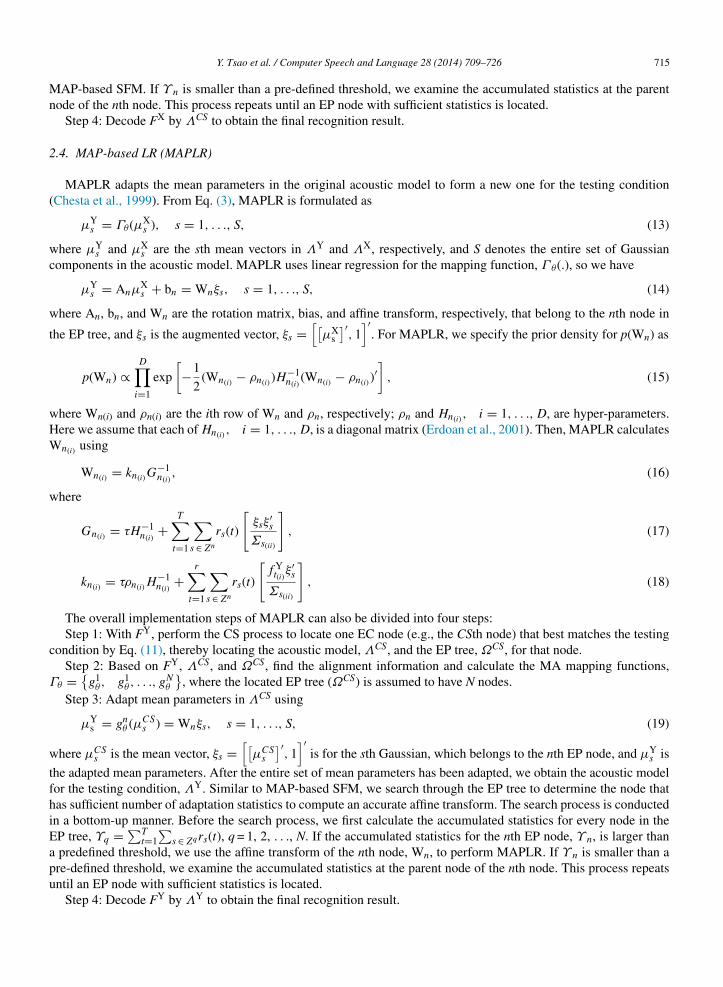
.4. MAP-based LR (MAPLR)

MAPLR adapts the mean parameters in the original acoustic model to form a new one for the testing conditionChesta et al., 1999). From Eq. (3), MAPLR is formulated as

μYs = Γθ(μX

s ), s = 1, . . ., S, (13)

here μYs and μX

s are the sth mean vectors in ΛY and ΛX, respectively, and S denotes the entire set of Gaussianomponents in the acoustic model. MAPLR uses linear regression for the mapping function, Γ θ(.), so we have

μYs = Anμ

Xs + bn = Wnξs, s = 1, . . ., S, (14)

here An, bn, and Wn are the rotation matrix, bias, and affine transform, respectively, that belong to the nth node in

he EP tree, and ξs is the augmented vector, ξs =[[

μXs

]′, 1

]′. For MAPLR, we specify the prior density for p(Wn) as

p(Wn) ∝D∏

i=1

exp

[−1

2(Wn(i) − ρn(i) )H

−1n(i)

(Wn(i) − ρn(i) )′]

, (15)

here Wn(i) and ρn(i) are the ith row of Wn and ρn, respectively; ρn and Hn(i) , i = 1, . . ., D, are hyper-parameters.ere we assume that each of Hn(i) , i = 1, . . ., D, is a diagonal matrix (Erdoan et al., 2001). Then, MAPLR calculatesn(i) using

Wn(i) = kn(i)G−1n(i)

, (16)

here

Gn(i) = τH−1n(i)

+T∑

t=1

∑s ∈ Zn

rs(t)

[ξsξ

′s

Σs(ii)

], (17)

kn(i) = τρn(i)H−1n(i)

+r∑

t=1

∑s ∈ Zn

rs(t)

[f Y

t(i)ξ′s

Σs(ii)

], (18)

The overall implementation steps of MAPLR can also be divided into four steps:Step 1: With FY, perform the CS process to locate one EC node (e.g., the CSth node) that best matches the testing

ondition by Eq. (11), thereby locating the acoustic model, ΛCS, and the EP tree, ΩCS, for that node.Step 2: Based on FY, ΛCS, and ΩCS, find the alignment information and calculate the MA mapping functions,

θ = {g1

θ, g1θ, . . ., gN

θ

}, where the located EP tree (ΩCS) is assumed to have N nodes.

Step 3: Adapt mean parameters in ΛCS using

μYs = gn

θ (μCSs ) = Wnξs, s = 1, . . ., S, (19)

here μCSs is the mean vector, ξs =

[[μCS

s

]′, 1

]′is for the sth Gaussian, which belongs to the nth EP node, and μY

s is

he adapted mean parameters. After the entire set of mean parameters has been adapted, we obtain the acoustic modelor the testing condition, ΛY. Similar to MAP-based SFM, we search through the EP tree to determine the node thatas sufficient number of adaptation statistics to compute an accurate affine transform. The search process is conductedn a bottom-up manner. Before the search process, we first calculate the accumulated statistics for every node in theP tree, Υq = ∑T

t=1∑

s ∈ Zqrs(t), q = 1, 2, . . ., N. If the accumulated statistics for the nth EP node, Υ n, is larger than

predefined threshold, we use the affine transform of the nth node, Wn, to perform MAPLR. If Υ n is smaller than are-defined threshold, we examine the accumulated statistics at the parent node of the nth node. This process repeatsntil an EP node with sufficient statistics is located.

Step 4: Decode FY by ΛY to obtain the final recognition result.

716 Y. Tsao et al. / Computer Speech and Language 28 (2014) 709–726

Although FC and MA can be used to compensate the same mismatch factors (or sources), they may be complementaryto each other, since they deal with the mismatch problem using different strategies. Therefore, the two approaches canbe integrated in an iterative manner to achieve further improvements. More details about the integration of FC and MAwill be presented in Section 4.

3. Prior density specification based on the environment structuring framework

As introduced in Sections 2.3 and 2.4, both MAP-based SFM and MAPLR take account of the hierarchical treestructure to well fit the testing acoustic environments. In this section, we present to use the tree structure to specifysuitable hyper-parameters of the prior densities for MAP-based SFM and MAPLR. Four types of prior densities aredeveloped and introduced in the following discussion.

3.1. Four types of prior densities

With the environment structuring framework, we can prepare clustered prior (CP), sequential prior (SP), hierarchicalprior (HP), and integrated prior (IP) densities for MAP-based SFM and MAPLR.

3.1.1. Clustered prior (CP)The hyper-parameters of the clustered prior (CP) density are estimated directly from the clustered data in each EP

node of the hierarchical tree. In the following, we assume that the cth EC node is selected, and the correspondingtraining data for this node is Qc. Next, we further assume that the cth EC node includes training data from K differentspeaker and speaking environments. Accordingly, we can divide Qc into K subsets of training data {Qc,1, Qc,2, . . .,Qc,K}. With these K subsets of training data, the CP densities of the MAP-based SFM and MAPLR in the cth EC nodeare computed as follows.

3.1.1.1. For MAP-based SFM. Step 1: Apply ML-based SFM to calculate K sets of compensation biases{δ1

n, δ2n, . . ., δK

n }, using the data from K different environments, namely {Qc,1, Qc,2, . . ., Qc,K}.Step 2: Estimate the hyper-parameters of the CP density (mean and covariance), {ηCP

n , VCPn } using

ηCPn(i)

= 1

K

K∑k=1

δkn(i)

, (20)

VCPn(ii)

= 1

K

K∑k=1

(δkn(i)

− ηCPn(i)

)2. (21)

3.1.1.2. For MAPLR. Step 1: Apply MLLR to calculate K sets of transformations, {W1n, W2

n, . . ., WKn }, using the data

from K different environments, namely {Qc,1, Qc,2, . . ., Qc,K}.Step-2: Obtain the hyper-parameters in the CP density {ρCP

n , HCPn } using

ρCPn(i)

= 1

K

K∑k=1

Wkn(i)

, (22)

(HCPn(i)

)jj

= 1

K

K∑k=1

(Wkn(ij)

− ρCPn(ij)

)2, (23)

where Wkn(ij)

and ρCPn(ij)

are the (ij)th elements of Wkn and ρCP

n , respectively, and (HCPn(i)

)jj

is the jjth diagonal element in

HCPn(i)

.

With the same procedure, we can estimate the CP density for every node in all of the C EP trees. Because each CP

density corresponds to a specific group of mean parameters for a particular cluster of environments, it provides localinformation of the ensemble environments. With the online CS process, we can directly locate the CP densities thatbest match the testing condition for MAP-based SFM and MAPLR.

3

(fhupm

3ec

c

p

3nb

c

h

r

wtpcSSa

3

me

3idl

Mn

3nu

Y. Tsao et al. / Computer Speech and Language 28 (2014) 709–726 717

.1.2. Sequential prior (SP)The hyper-parameters of the sequential prior (SP) density are estimated based on sequential Bayesian learning

Hamilton, 1991). The SP densities enable MAP-based SFM and MAPLR to incorporate information seen previouslyor compensating the current testing utterances and for adapting the current acoustic model. The use of the SP densityas been confirmed effective for MAP-based SFM (Jiang et al., 2001; Tsao et al., 2011); here we refine it further bysing the local information provided by the environment structuring framework. In our system, the CS procedure iserformed first to locate the acoustic model and EP tree that best match the testing utterance. With the located acousticodel and EP tree, the SP densities for MAP-based SFM and MAPLR are estimated through the following steps.

.1.2.1. For MAP-based SFM. Step 1: At the beginning stage, initialize the hyper-parameters in the SP densities forvery EP node. The hyper-parameter for the nth EP node is initialized as {ηSP(0)

n = 0}. For the first utterance, δ(1)n is

omputed based on the ML criterion using Eqs. (8)–(10) while setting � = 0 in Eqs. (9) and (10).Step 2: For the uth utterance, use the SP density with ηSP(u−1)

n , estimated from the previous (u − 1) utterances, toalculate δ(u)

n using Eqs. (8)–(10).Step 3: Use the calculated δ(u)

n to update the hyper-parameters for the following utterances. Accordingly, the hyper-arameter for the nth EP node becomes {ηSP(u)

n = δ(u)n }.

.1.2.2. For MAPLR. Step 1: At the beginning stage, initialize the hyper-parameters in the SP densities for every EPode. The hyper-parameter for the nth EP node is initialized as {ρSP(0)

n = 0}. For the first utterance, W(1)n is computed

ased on the ML criterion using Eqs. (16)–(18) while setting τ = 0 in Eqs. (17) and (18).Step 2: For the uth utterance, use the SP density with ρSP(u−1)

n , estimated from the previous (u − 1) utterances, toalculate W(u)

n using Eqs. (16)–(18).Step-3: Use the calculated W(u)

n to update the hyper-parameters for the following utterances. Accordingly, theyper-parameter for the nth EP node becomes {ρSP(u)

n = W(u)n }.

To simplify the online computation, we only sequentially update ηSP(u)n and ρSP(u)

n for MAP-based SFM and MAPLR,espectively, and use fixed VSP

n and HSPn in the online process. Here, we set VSP

n = VCPn and HSP

n = HCPn .

Although the SP density can effectively utilize the information from previous testing data to perform FC and MA,hen the environment condition changes abruptly (for example, from high SNR to low SNR conditions), the use of

he SP density may lead to poor FC and MA mapping function estimations. Therefore in our study, the CS process iserformed before using the SP density to prevent the performance degradations caused by sudden acoustic conditionhanges. By performing the CS process, only the most suitable EP tree is selected for each testing utterance, and theP density of that EP tree is used for the MAP-based estimations. After decoding on that utterance, we only update theP density of that selected EP tree for the following utterances. In this sense, only the suitable SP densities are usednd updated for each particular test utterance.

.1.3. Hierarchical prior (HP)As in the case of the SP densities, we perform the CS process to locate the acoustic model and EP tree that best

atch the testing condition to calculate the HP densities. The HP densities for MAP-based SFM and MAPLR arestimated as follows.

.1.3.1. For MAP-based SFM. Step 1: For the root node of the EP tree, we calculate δ1 using the entire set of meansn the root node based on the ML criterion using Eqs. (8)–(10) while setting � = 0 in Eqs. (9) and (10), where no HPensity is used in the calculation. The estimated δ1 is used to prepare the prior densities for the child nodes in the nextayer.

Step 2: For the nth node with its parent node r (as shown in Fig. 3), we have the hyper-parameter ηSPn = δr, and

AP-based SFM calculates δn using Eqs. (8)–(10). The calculated δn is used to prepare the prior densities for the childodes of the nth node.

Step 3: Repeat Step 2 until reaching the leaf nodes of the EP tree.

.1.3.2. For MAPLR. Step 1: For the root node of the EP tree, we calculate W1 using the entire set of means in the rootode based on the ML criterion using Eqs. (16)–(18) while setting τ = 0 in Eqs. (17) and (18), where no HP density issed in the calculation. The calculated W1 is used as the prior densities for the child nodes in the next layer.

718 Y. Tsao et al. / Computer Speech and Language 28 (2014) 709–726

Step 2: For the nth node with its parent node r (as shown in Fig. 3), we have the hyper-parameter ρHPn = Wr, and

MAPLR calculates Wn using Eqs. (16)–(18). The calculated Wn is used to prepare the prior densities for the childnodes of the nth node.

Step 3: Repeat Step 2 until reaching the leaf nodes of the EP tree.As in the case of the SP densities, we only online estimate mean hyper-parameters, ηHP

n and ρHPn for MAP-based

SFM and MAPLR, respectively, and use fixed VHPn (= VCP

n ) and HHPn (= HCP

n ). The main advantage of the HP densitiesis that the information of the current testing utterance can be used efficiently with the EP tree structure.

3.1.4. Integrated prior (IP)The hyper-parameters in the IP densities combine those in the three prior densities presented above. We simply use

a linear combination in this study. Therefore, for MAP-based SFM, we obtain the hyper-parameter, ηIPn , using:

ηIPn = wCPηCP

n + wSPηSPn + wHPηHP

n , (24)

where WCP, WSP, and WHP are weighting coefficients.Similarly for MAPLR, we obtain the hyper-parameter, ρIP

n , using:

ρIPn = εCPρCP

n + εSPρSPn + εHPρHP

n , (25)

where εCP, εSP, and εHP are weighting coefficients. In this study, we only update ηIPn and ρIP

n , respectively, for MAP-based SFM and MAPLR online, and use fixed VIP

n (= VCPn ) and HIP

n (= HCPn ). As in the case of the HP densities,

we first locate one EP tree, and then iteratively estimate and propagate the IP densities. Finally, the estimation andpropagation stop at the leaf nodes of the EP tree. Notably, the CP, SP, and HP densities are estimated using theinformation from the training data, statistics seen from the previous utterances, and the current testing data with theEP tree, respectively. Therefore, the IP densities incorporate multiple prior information sources.

4. Experiments

In this section, we present the speech databases, experimental setup, and results of MAP-based FC and MA withthe environment structuring framework.

4.1. Speech databases

We conducted experiments on two sets of speech tasks, Aurora-2 (Pearce and Hirsch, 2000; Macho et al., 2002) andAurora-4 (Hirsch, 2001; Parihar and Picone, 2002; Parihar et al., 2004). Aurora-2 is a connected digit recognition taskincluding two training sets, multi-condition and clean condition. The multi-condition training set was used to buildacoustic models and to construct the environment structuring framework. There are 70 different testing conditions (tennoise types at seven SNR levels) in Aurora-2. These 70 testing conditions were divided into set A, set B, and set C.Speech signals in test sets A and B were distorted by additive noises (in set A, the noise types were subway, babble, car,and exhibition; in set B, the noise types were restaurant, street, airport, and train station). Speech signals in set C weredistorted by additive noise and channel effects (subway and street noises together with an MIRS channel mismatch).

Speech data in the Aurora-4 task were obtained from the Wall Street Journal (WSJ0) database (Paul and Baker,1992) and artificially contaminated with different types of noise at SNR levels ranging from 5 to 15 dB. Two samplingrates, 8 kHz and 16 kHz, were available for both training and testing. In this study, the 8 kHz sampling rate conditionwas used. The multi-condition training set was selected to build acoustic models and to construct the environmentstructuring framework. This training set included 7138 utterances. Fourteen test sets were provided for evaluatingperformances, and 166 utterances for each test set were used as suggested in (Parihar and Picone, 2002). The 14 testsets were classified into four groups: set A (clean data with matched channel condition to the training data; test set 1),

set B (noisy data with matched channel condition to the training data; test sets 2–7), set C (clean data with mismatchedchannel condition to the training data; test set 8), and set D (noisy data with mismatched channel condition to thetraining data; test sets 9–14). In the following, we will present performances of these four sets along with an averageresult, Avg (test sets 1–14).

Y. Tsao et al. / Computer Speech and Language 28 (2014) 709–726 719

Train

UBM

MAP

Adapt .

VQTrai ning

SpeechGMM

UBM

1-st

GMM

2-nd

GMM

K-1

GMM

(1)

(2)

(4)

Uth

GMM

(3)

1st 2nd Uth

4

EdAs(o

ddattbbmpdt

iuIsntAldodtoS

ut

U

Fig. 4. Environment clustering procedure.

.2. Experimental setup

For both Aurora-2 and Aurora-4, we used the ETSI advanced front-end (AFE) for feature extraction (ETSI, 2007).ach feature vector comprised 39 dimensions including 13 static features along with their first- and second-orderynamic features. To perform speech recognition, the HVite function in HTK toolkit (Young et al., 2005) was used forurora-2. On the other hand, for Aurora-4, we used a weighted finite state transducer (WFST) (Mohri et al., 2008) based

peech recognizer that was developed at National Institute of Information and Communications Technology (NICT)Dixon et al., 2012). Here, we intentionally used two types of decoders to confirm the compatibility of MAP-based FCr/and MA with the environment structuring framework and different ASR systems.

For Aurora-2, we followed the complex backend HMM topology suggested by (Macho et al., 2002) to prepare 11igit models (zero, one, two, three, four, five, six, seven, eight, nine, and oh) with silence and short pause models. Eachigit model contained 16 states and 20 Gaussian mixtures per state. Silence and short pause models included threend one states, respectively, and 36 mixtures per state. For Aurora-4, we adopted a triphone-based HMM topologyo train acoustic models. For this topology, we used 2137 shared states in total. Each triphone was characterized byhree active states, and each state was modeled by eight Gaussians. Silence and short pause were also characterizedy three active states, where each state was characterized by 16 Gaussians. In the original Aurora-4 baseline system, aigram language model was used to test recognition (Parihar et al., 2004). In more recent studies, a trigram languageodel has also been used to provide more powerful language modeling capability and thus achieve better recognition

erformance (Hilger and Ney, 2006; Tüske et al., 2011). When using a trigram language model, it becomes moreifficult to further improve the recognition performance than using a bigram language model. In this study, we used arigram back-off language model that was prepared by the reference transcription of the training utterances.

For each of the Aurora-2 and Aurora-4 tasks, we constructed an environment structuring framework (in Fig. 2),ncluding one two-layer EC and one two-layer EP tree. The root node of the EC tree contained the entire set of trainingtterances. In the first layer, the EC tree included two nodes, dividing the entire set of training data into two clusters.n the second layer, each node in the first layer was further divided into two nodes, with each node containing aubset of training data from its parent node. Finally, an EC tree with seven nodes (one root node, two intermediateodes, and four leaf nodes) was constructed. In the proposed framework, data clustering units can be any particularypes, which correspond to underlying distortion factors that cause mismatches of training and testing conditions. Forurora-2 and Aurora-4, speaker variability, noise types, and SNR conditions are obvious distortion factors. When the

abels corresponding to these distortions are available, data clustering can be performed accordingly. In the Aurora-2atabase, the training set included 17 different speaking environments that were originated form the same four typesf noise as in test set A, at four SNR levels: 5 dB, 10 dB, 15 dB, and 20 dB, along with clean condition. We furtherivided the training set into two gender-specific subsets to form 34 speaker and speaking environments. In this study,he two-layer EC tree used in Aurora-2 was constructed by: the first layer classified the 34 environments into two groupsf two genders, and the second layer separated the 17 environments into two groups roughly according to high/lowNR levels (Tsao et al., 2011).

On the other hand, the training data in Aurora-4 did not provide explicit SNR labels, and thus we adopted antterance level clustering process to build the EC tree. The following four steps were performed to construct the EC

ree (as presented in Fig. 4):

Step 1: Use the entire training set to estimate a Gaussian mixture model-based universal background model (GMM-BM).

720 Y. Tsao et al. / Computer Speech and Language 28 (2014) 709–726

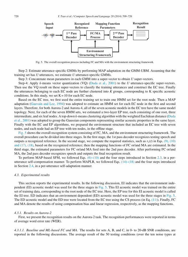
Fig. 5. The overall recognition process including FC and MA with the environment structuring framework.

Step 2: Estimate utterance-specific GMMs by performing MAP adaptation on the GMM-UBM. Assuming that thetraining set has U utterances, we estimate U utterance-specific GMMs.

Step 3: Concatenate mean parameters in each GMM into a super-vector to obtain U super-vectors.Step-4: Apply k-means vector quantization (VQ) (Duda et al., 2001) to the U utterance-specific super-vectors.

Then use the VQ result on these super-vectors to classify the training utterances and construct the EC tree. Finallythe utterances belonging to each EC node are further clustered into K groups, corresponding to K specific acousticconditions. In this study, we set K = 10 for each EC node.

Based on the EC tree, we first used the entire training set to train one HMM set for the root node. Then a MAPadaptation (Gauvain and Lee, 1994) was adopted to estimate an HMM set for each EC node in the first and secondlayers. Therefore, for both Aurora-2 and Aurora-4, all of the seven acoustic models in the EC tree have the same modeltopology. Next, for each of the seven HMM sets, we estimated a two-layer EP tree, each consisting of one root, threeintermediate, and six leaf nodes. A top-down k-means clustering algorithm with the weighted Euclidean distance (Dudaet al., 2001) was adopted to group the Gaussian components representing similar acoustic properties in the same layer.Finally with the EC and EP algorithms, we prepared the environment structure that included an EC tree with sevennodes, and each node had an EP tree with ten nodes, in the offline stage.

Fig. 5 shows the overall recognition system consisting of FC, MA, and the environment structuring framework. Theoverall procedure can be divided into three stages. In the first stage, the 1st pass decoder recognizes testing speech andoutputs a recognized reference. In the second stage, we compute the required statistics, such as rs(t) in Eqs. (9), (10)and (17), (18), based on the recognized reference; then the mapping functions of FC or/and MA are estimated. In thethird stage, the estimated parameters for FC or/and MA feed into the 2nd pass decoder. After performing FC or/andMA, the 2nd pass decoder recognizes speech and outputs the final recognition result.

To perform MAP-based SFM, we followed Eqs. (6)–(10) and the four steps introduced in Section 2.3, in a per-utterance self-compensation manner. To perform MAPLR, we followed Eqs. (14)–(18) and the four steps introducedin Section 2.4, in a per-utterance self-adaptation manner.

4.3. Experimental results

This section reports the experimental results. In the following discussion, EI indicates that the environment inde-pendent (EI) acoustic model was used for the three stages in Fig. 5. This EI acoustic model was trained on the entireset of training data, corresponding to the root node of the EC tree. Here, the EP tree for this EI acoustic model is calledthe EI tree. ED indicates that an environment dependent (ED) acoustic model was used for the three stages in Fig. 5.The ED acoustic model and the ED tree were located from the EC tree using the CS process (in Eq. (11)). Finally, FCand MA denote the results of using compensation bias and linear regression, respectively, as the mapping functions.

4.3.1. Results on Aurora-2First, we present the recognition results on the Aurora-2 task. The recognition performances were reported in terms

of average word error rate (WER).

4.3.1.1. Baseline and ML-based FC and MA. The results for sets A, B, and C, in 0- to 20-dB SNR conditions, arereported in the following discussions. The average result of the 50 testing conditions (over the ten noise types at

Y. Tsao et al. / Computer Speech and Language 28 (2014) 709–726 721

Table 1WER (%) of baseline (EI) and ML-based FC (EI) and MA (EI) on Aurora-2.

Test condition Set A Set B Set C Avg

Baseline (EI) 5.92 6.69 7.11 6.46ML-FC (EI) 5.88 6.57 6.97 6.37ML-MA (EI) 5.65 6.20 6.33 6.01

Table 2WER (%) of baseline (ED) and ML-based FC (ED) and MA (ED) on Aurora-2.

Test condition Set A Set B Set C Avg

Baseline (ED) 5.11 5.51 6.42 5.53ML-FC (ED) 5.10 5.48 6.40 5.51M

0aaw(b

MpMtio

4iAfε

L-MA (ED) 5.03 5.40 5.79 5.33

- to 20-dB SNR levels) is also provided as Avg. We list the EI experimental results of the Baseline, ML-based FC,nd ML-based MA, respectively, as Baseline (EI), ML-FC (EI), and ML-MA (EI) in Table 1. Notably, ML-based FCnd MA, respectively, use � = 0 in Eqs. (9) and (10) and τ = 0 in Eqs. (17) and (18). For Baseline (EI) in Table 1,e directly use the EI acoustic model to test recognition. The same baseline results can be found in previous studies

Wu and Huo, 2006; Tsao and Lee, 2009). The results in Table 1 verified that both ML-FC and ML-MA improved theaseline performance consistently over sets A, B, C, and Avg.

Next, we list the ED results of the Baseline, ML-based FC, and ML-based MA, respectively, as Baseline (ED),L-FC (ED), and ML-MA (ED) in Table 2. For this set of results, we used the ED acoustic model and ED tree to

erform ML-FC, ML-MA, and test recognition. From Table 2, we observe clear improvements of ML-FC (ED) andL-MA (ED) over Baseline (ED). Comparing Tables 1 and 2, we notice that we can obtain better performance for

he baseline, FC, and MA using the ED acoustic model and ED tree than using the EI acoustic model and EI tree. Themprovements confirm the benefits of using the ED acoustic model and ED tree that incorporate the local informationf the environment space.

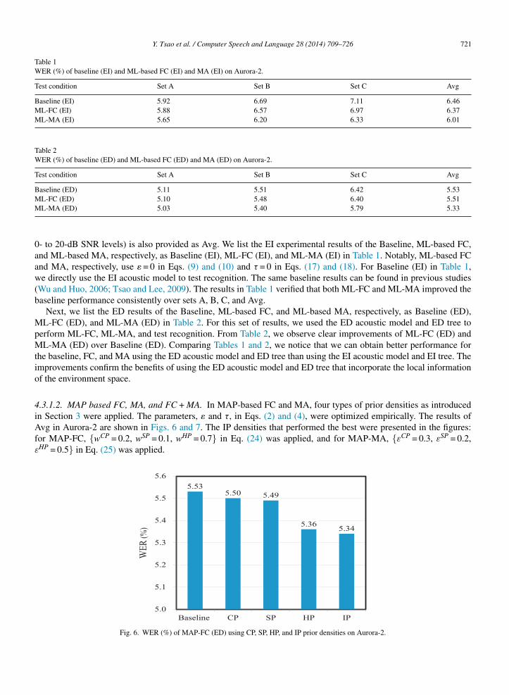
.3.1.2. MAP based FC, MA, and FC + MA. In MAP-based FC and MA, four types of prior densities as introducedn Section 3 were applied. The parameters, � and τ, in Eqs. (2) and (4), were optimized empirically. The results ofvg in Aurora-2 are shown in Figs. 6 and 7. The IP densities that performed the best were presented in the figures:

or MAP-FC, {wCP = 0.2, wSP = 0.1, wHP = 0.7} in Eq. (24) was applied, and for MAP-MA, {εCP = 0.3, εSP = 0.2,HP = 0.5} in Eq. (25) was applied.

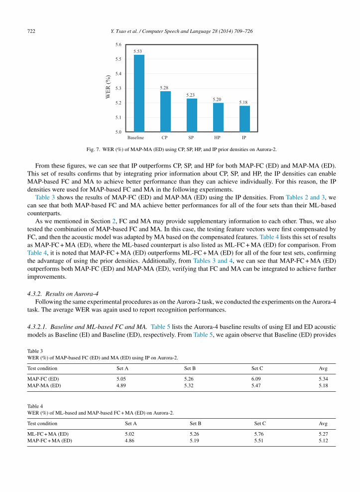
Fig. 6. WER (%) of MAP-FC (ED) using CP, SP, HP, and IP prior densities on Aurora-2.

722 Y. Tsao et al. / Computer Speech and Language 28 (2014) 709–726

5.53

5.28

5.235.20

5.18

5.0

5.1

5.2

5.3

5.4

5.5

5.6

WE

R (

%)

Baseline CP SP HP IP

Fig. 7. WER (%) of MAP-MA (ED) using CP, SP, HP, and IP prior densities on Aurora-2.

From these figures, we can see that IP outperforms CP, SP, and HP for both MAP-FC (ED) and MAP-MA (ED).This set of results confirms that by integrating prior information about CP, SP, and HP, the IP densities can enableMAP-based FC and MA to achieve better performance than they can achieve individually. For this reason, the IPdensities were used for MAP-based FC and MA in the following experiments.

Table 3 shows the results of MAP-FC (ED) and MAP-MA (ED) using the IP densities. From Tables 2 and 3, wecan see that both MAP-based FC and MA achieve better performances for all of the four sets than their ML-basedcounterparts.

As we mentioned in Section 2, FC and MA may provide supplementary information to each other. Thus, we alsotested the combination of MAP-based FC and MA. In this case, the testing feature vectors were first compensated byFC, and then the acoustic model was adapted by MA based on the compensated features. Table 4 lists this set of resultsas MAP-FC + MA (ED), where the ML-based counterpart is also listed as ML-FC + MA (ED) for comparison. FromTable 4, it is noted that MAP-FC + MA (ED) outperforms ML-FC + MA (ED) for all of the four test sets, confirmingthe advantage of using the prior densities. Additionally, from Tables 3 and 4, we can see that MAP-FC + MA (ED)outperforms both MAP-FC (ED) and MAP-MA (ED), verifying that FC and MA can be integrated to achieve furtherimprovements.

4.3.2. Results on Aurora-4Following the same experimental procedures as on the Aurora-2 task, we conducted the experiments on the Aurora-4

task. The average WER was again used to report recognition performances.

4.3.2.1. Baseline and ML-based FC and MA. Table 5 lists the Aurora-4 baseline results of using EI and ED acousticmodels as Baseline (EI) and Baseline (ED), respectively. From Table 5, we again observe that Baseline (ED) provides

Table 3WER (%) of MAP-based FC (ED) and MA (ED) using IP on Aurora-2.

Test condition Set A Set B Set C Avg

MAP-FC (ED) 5.05 5.26 6.09 5.34MAP-MA (ED) 4.89 5.32 5.47 5.18

Table 4WER (%) of ML-based and MAP-based FC + MA (ED) on Aurora-2.

Test condition Set A Set B Set C Avg

ML-FC + MA (ED) 5.02 5.26 5.76 5.27MAP-FC + MA (ED) 4.86 5.19 5.51 5.12

Y. Tsao et al. / Computer Speech and Language 28 (2014) 709–726 723

Table 5WER (%) of baseline (EI) and baseline (ED) on Aurora-4.

Test set Set A Set B Set C Set D Avg

Baseline (EI) 9.94 17.24 13.33 22.89 18.86Baseline (ED) 9.10 15.80 11.93 22.32 17.84

Table 6WER (%) of ML-based FC (ED), MA (ED), and FC + MA (ED) on Aurora-4.

Test set Set A Set B Set C Set D Avg

ML-FC (ED) 9.36 15.52 11.09 21.68 17.41ML-MA (ED) 9.13 16.16 11.53 21.73 17.71ML-FC + MA (ED) 9.02 15.90 11.38 21.86 17.64

Table 7WER (%) of MAP-based FC (ED), MA (ED), and FC + MA (ED) on Aurora-4.

Test set Set A Set B Set C Set D Avg

MAP-FC (ED) 9.21 15.43 11.03 21.25 17.16MM

cd

aMMo

4beu

oeF(Fpa

4mEuoi

F

AP-MA (ED) 8.84 15.61 11.53 21.12 17.20AP-FC + MA (ED) 8.91 15.39 11.34 21.05 17.06

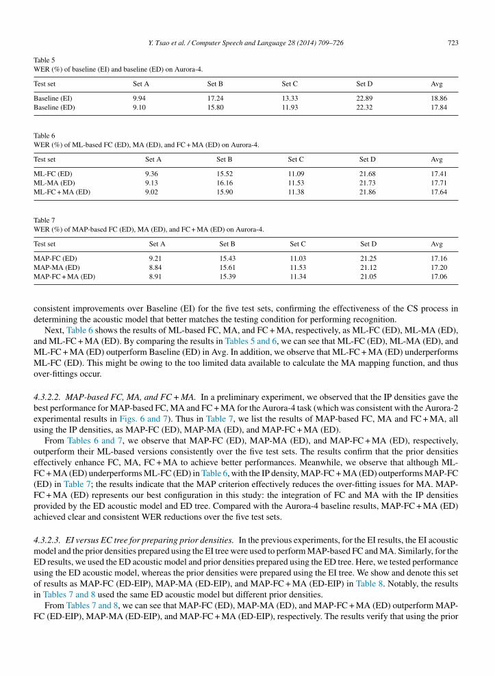
onsistent improvements over Baseline (EI) for the five test sets, confirming the effectiveness of the CS process inetermining the acoustic model that better matches the testing condition for performing recognition.

Next, Table 6 shows the results of ML-based FC, MA, and FC + MA, respectively, as ML-FC (ED), ML-MA (ED),nd ML-FC + MA (ED). By comparing the results in Tables 5 and 6, we can see that ML-FC (ED), ML-MA (ED), andL-FC + MA (ED) outperform Baseline (ED) in Avg. In addition, we observe that ML-FC + MA (ED) underperformsL-FC (ED). This might be owing to the too limited data available to calculate the MA mapping function, and thus

ver-fittings occur.

.3.2.2. MAP-based FC, MA, and FC + MA. In a preliminary experiment, we observed that the IP densities gave theest performance for MAP-based FC, MA and FC + MA for the Aurora-4 task (which was consistent with the Aurora-2xperimental results in Figs. 6 and 7). Thus in Table 7, we list the results of MAP-based FC, MA and FC + MA, allsing the IP densities, as MAP-FC (ED), MAP-MA (ED), and MAP-FC + MA (ED).

From Tables 6 and 7, we observe that MAP-FC (ED), MAP-MA (ED), and MAP-FC + MA (ED), respectively,utperform their ML-based versions consistently over the five test sets. The results confirm that the prior densitiesffectively enhance FC, MA, FC + MA to achieve better performances. Meanwhile, we observe that although ML-C + MA (ED) underperforms ML-FC (ED) in Table 6, with the IP density, MAP-FC + MA (ED) outperforms MAP-FCED) in Table 7; the results indicate that the MAP criterion effectively reduces the over-fitting issues for MA. MAP-C + MA (ED) represents our best configuration in this study: the integration of FC and MA with the IP densitiesrovided by the ED acoustic model and ED tree. Compared with the Aurora-4 baseline results, MAP-FC + MA (ED)chieved clear and consistent WER reductions over the five test sets.

.3.2.3. EI versus EC tree for preparing prior densities. In the previous experiments, for the EI results, the EI acousticodel and the prior densities prepared using the EI tree were used to perform MAP-based FC and MA. Similarly, for theD results, we used the ED acoustic model and prior densities prepared using the ED tree. Here, we tested performancesing the ED acoustic model, whereas the prior densities were prepared using the EI tree. We show and denote this setf results as MAP-FC (ED-EIP), MAP-MA (ED-EIP), and MAP-FC + MA (ED-EIP) in Table 8. Notably, the results

n Tables 7 and 8 used the same ED acoustic model but different prior densities.

From Tables 7 and 8, we can see that MAP-FC (ED), MAP-MA (ED), and MAP-FC + MA (ED) outperform MAP-C (ED-EIP), MAP-MA (ED-EIP), and MAP-FC + MA (ED-EIP), respectively. The results verify that using the prior

724 Y. Tsao et al. / Computer Speech and Language 28 (2014) 709–726

Table 8WER (%) of MAP-FC (ED-EIP), MAP-MA (ED-EIP), and MAP-FC+MA (ED-EIP) on Aurora-4.

Test set Set A Set B Set C Set D Avg

MAP-FC (ED-EIP) 9.17 15.46 10.98 21.40 17.24MAP-MA (ED-EIP) 9.06 15.97 11.42 21.34 17.45MAP-FC + MA (ED-EIP) 8.91 15.62 11.34 21.18 17.22

Table 9P-values of MAP-FC (ED), MAP-MA (ED), and MAP-FC + MA (ED) versus MAP-FC (ED-EIP), MAP-MA (ED-EIP), and MAP-FC + MA(ED-EIP) on Aurora-4.

MAP-FC (ED) MAP-MA (ED) MAP-FC + MA (ED)

MAP-FC (ED-EIP) 0.014 – –MAP-MA (ED-EIP) – 0.023 –

MAP-FC + MA (ED-EIP) – – 0.021

densities prepared by the ED tree, MAP-based FC, MA, and FC + MA can yield better performance than that usingprior densities prepared using the EI tree.

We intend to further verify the significance of improvements (WER reductions) of MAP-FC (ED), MAP-MA (ED),and MAP-FC + MA (ED) over MAP-FC (ED-EIP), MAP-MA (ED-EIP), and MAP-FC + MA (ED-EIP), using a t-testanalysis (Hayter, 2006). Because the entire Aurora-4 test set has 14 different sets, we conducted the t-test on 14pair-wise results. Table 9 lists the t-test results of MAP-based FC, MA, and FC + MA using prior densities preparedusing the EI tree versus that prepared using the ED tree. From Table 9, we observe small p-values for the t-testresults, suggesting that MAP-FC (ED), MAP-MA (ED), and MAP-FC + MA (ED), respectively, outperform MAP-FC(ED-EIP), MAP-MA (ED-EIP), and MAP-FC + MA (ED-EIP), over the 14 test sets consistently. Since the ED treeprovides local information, the results confirm that more suitable prior densities can be designed by incorporating localinformation to enable MAP-based algorithms to achieve better performance.

5. Conclusion

In this paper, we proposed a two-stage environment structuring framework to facilitate suitable prior density spec-ification for MAP-based FC and MA for robust speech recognition. Based on the EC and EP processes, a hierarchicaltree structure was created to describe the acoustic environments. Based on the hierarchical tree structure, we candetermine a local acoustic space to fit the testing condition. In addition, based on the hierarchical tree structure, weproposed three types of prior density estimation algorithms as well as their combination to facilitate the MAP-basedFC and MA. On the Aurora-2 and Aurora-4 tasks, our evaluation showed that by using the environment structuringframework to determine the best acoustic model for recognition, we can already improve the baseline recognitionresults. Moreover, the performance can be enhanced by adopting ML-based FC and MA. A further improvement wasachieved by using MAP-based FC and MA. In addition, from the results of utilizing the prior density estimation forMAP-based FC and MA, we confirmed that the IP densities gave the best performance, because they integrated theknowledge of prior information sources from the CP, HP, and SP densities. Finally, considering the contributions of theED and EI trees for robust recognition, we observed that using the prior densities prepared by the ED tree outperformedthat prepared by the EI tree. All of these results confirmed the advantage of incorporating local information into priordensity preparation.

In this study, we focused our attention on using the environment structuring framework to prepare suitable priordensities for MAP-based FC and MA. Only MAP-based SFM and MAPLR were presented as two application examples.It is clear that other MAP-based approaches can also utilize the prior densities prepared by the environment structuring

framework. Additionally, the proposed framework can be applied to other tasks, such as environment or event modelingand de-noising for audio event recognition tasks, and speaker modeling for speaker recognition tasks. We will explorefurther in these directions in the future.

A

M

R

AB

C

C

C

C

DDDEE

E

EE

GGG

GH

H

H

HHH

H

H

H

H

I

J

JJ

J

Y. Tsao et al. / Computer Speech and Language 28 (2014) 709–726 725

cknowledgement

This work was supported by the National Science Council of Taiwan under contracts NSC101-2221-E-001-020-Y3.

eferences

cero, A., 1990. Acoustical and Environmental Robustness in Automatic Speech Recognition. Carnegie Mellon University (Ph.D. Thesis).oll, S.F., 1979. Suppression of acoustic noise in speech using spectral subtraction. IEEE Transactions on Acoustics Speech and Signal Processing

27 (2), 113–120.hen, C.-P., Bilmes, J.A., Kirchhoff, K., 2002a. Lowresource noise-robust feature post-processing on aurora 2.0. In: Proc. ICSLP’02,

pp. 2445–2448.hen, C.-P., Filali, K., Bilmes, J.A., 2002b. Frontend post-processing and backend model enhancement on the aurora 2.0/3.0 databases. In: Proc.

ICSLP’02, pp. 241–244.hen, J., Benesty, J., Huang, Y., Diethorn, E., 2007. Fundamentals of Noise Reduction in Spring Handbook of Speech Processing. Springer-Verlag,

Berlin.hesta, C., Siohan, O., Lee, C.-H., 1999. Maximum a posteriori linear regression for hidden Markov model adaptation. In: Proc. Eurospeech’99,

pp. 211–214.eng, L., Huang, X., 2004. Challenges in adopting speech recognition. Communications of the ACM 47 (1), 69–75.ixon, P.R., Hori, C., Kashioka, H., 2012. A comparison of dynamic WFST decoding approaches. In: Proc. ICASSP’12, pp. 4209–4212.uda, R.O., Hart, P.E., Stork, D.G., 2001. Pattern Classification. Wiley, New York.phraim, Y., 1992. Statistical-model-based speech enhancement systems. Proceedings of IEEE 80 (10), 1526–1555.phraim, Y., Malah, D., 1984. Speech enhancement using a minimum mean-square error short-time spectral amplitude estimator. IEEE Transactions

on Acoustics Speech and Signal Processing 32 (6), 1109–1121.phraim, Y., Malah, D., 1985. Speech enhancement using a minimum mean-square error log-spectral amplitude estimator. IEEE Transactions on

Acoustics, Speech and Signal Processing 33 (2), 443–445.rdoan, H., Gao, Y., Picheny, M., 2001. Rapid adaptation using penalized-likelihood methods. In: Proc. ICASSP’01, pp. 333–336.TSI ES 202 050 V1.1.5, 2007. Speech processing, transmission and quality-aspects (STQ); distributed speech recognition; advanced frontend

feature extraction algorithms. In: ETSI Standard.ales, M.J.F., 1997. Maximum likelihood linear transformations for HMM-based speech recognition. In: Technical Report. Cambridge University.ales, M.J.F., 1996. The generation and use of regression class trees for MLLR adaptation. In: Technical Report. Cambridge University.auvain, J.-L., Lee, C.-H., 1994. Maximum a posteriori estimation for multivariate Gaussian mixture observations of Markov chains. IEEE

Transactions on Speech and Audio Processing 2 (2), 291–298.ong, Y., 1995. Speech recognition in noisy environments: a survey. Speech Communication 16 (3), 261–291.amilton, J.D., 1991. A quasi-Bayesian approach to estimating parameters for mixtures of normal distributions. Journal of Business & Economic

Statistics 9 (1), 27–39.ansen, J.H.L., Radhakrishnan, V., Arehart, K.H., 2006. Speech enhancement based on generalized minimum mean square error estimators and

masking properties of the auditory system. IEEE Transactions on Audio, Speech, and Language Processing 14 (6), 2049–2063.ansler, E., Schmidt, G., 2006. Topic in Acoustic Echo and Noise Control: Selected Methods for the Cancellation of Acoustical Echoes, the

Reduction of Background Noise, and Speech Processing (Signals and Communication Technology). Springer-Verlag, New York.ayter, A.J., 2006. Probability and Density for Engineers and Scientists. Duxbury Press, Belmont.ermansky, H., Morgan, N., 1994. RASTA processing of speech. IEEE Transactions on Speech and Audio Processing 2 (4), 578–589.ilger, F., Ney, H., 2006. Quantile based histogram equalization for noise robust large vocabulary speech recognition. IEEE Transactions on Audio,

Speech, and Language Processing 14 (3), 845–854.irsch, G., 2001. Experimental framework for the performance evaluation of speech recognition front-ends on a large vocabulary task. In: ETSI

STQ Aurora DSR Working Group.uang, X., Acero, A., Hon, H.-W., 2001. Spoken language processing: a guide to theory. In: Algorithm and System Development. Prentice Hall

PTR, New Jersy.uo, Q., Chan, C., Lee, C.-H., 1995. Bayesian adaptive learning of the parameters of hidden Markov model for speech recognition. IEEE Transactions

on Speech and Audio Processing 3 (5), 334–345.uo, Q., Lee, C.-H., 2000. A Bayesian predictive classification approach to robust speech recognition. IEEE Transactions on Speech and Audio

Processing 8 (2), 200–204.bm, D.P., Dharanipragada, S., Padmanabhan, M., 2000. A nonlinear unsupervised adaptation technique for speech recognition. In: Proc. ICSLP’00,

pp. 556–559.iang, H., Li, X., Liu, C., 2006. Large margin hidden Markov models for speech recognition. IEEE Transactions on Audio, Speech, and Language

Processing 14 (5), 1584–1595.iang, H., Soong, F., Lee, F., Lee, C.-H., 2001. Hierarchical stochastic matching for robust speech recognition. In: Proc. ICASSP’01, pp. 217–220.

uang, B.-H., Chou, W., Lee, C.-H., 1997. Minimum classification error rate methods for speech recognition. IEEE Transactions on Speech Audio

Processing 5 (3), 257–265.unqua, J.C., Haton, J.P., Wakita, H., 1996. Robustness in Automatic Speech Recognition: Fundamentals and applications. Kluwer Academic

Publishers, Boston.

726 Y. Tsao et al. / Computer Speech and Language 28 (2014) 709–726

Kim, H., Rose, R.C., 2003. Cepstrum-domain acoustic feature compensation based on decomposition of speech and noise for ASR in noisyenvironments. IEEE Transactions on Speech and Audio Processing 11 (5), 435–446.

Kjems, U., Jensen, J., 2012. Maximum likelihood based noise covariance matrix estimation for multi-microphone speech enhancement. In: Proc.EUSIPCO, pp. 295–299.

Lee, C.-H., 1998. On stochastic feature and model compensation approaches to robust speech recognition. Speech Communication 25 (1–3), 29–47.Leggetter, C., Woodland, P., 1995. Maximum likelihood linear regression for speaker adaptation of continuous density hidden Markov models.

Computer Speech and Language 9 (2), 171–185.Li, J., Yuan, M., Lee, C.-H., 2007. Approximate test risk bound minimization through soft margin estimation. IEEE Transactions on Audio, Speech,

and Language Processing 15 (8), 2393–2404.Li, Y., Erdogan, H., Gao, Y., Marcheret, E., 2002. Incremental online feature space mllr adaptation for telephony speech recognition. In: Proc.

ICSLP’02, pp. 1417–1420.Lotter, T., Vary, P., 2005. Speech enhancement by MAP spectral amplitude estimation using a super-Gaussian speech model. EURASIP Journal on

Applied Signal Processing 7, 1110–1126.Macho, D., Mauuary, L., Noe, B., Cheng, Y.M., Ealey, D., Jouver, D., Kelleher, H., Pearce, D., Saadoun, F., 2002. Evaluation of a noise-robust DSR

front-end on Aurora databases. In: Proc. ICSLP’02, pp. 17–20.Makhoul, J., 1976. Linear prediction: a tutorial review. Proceedings of IEEE 63 (2), 561–580.Martin, R., 2005. Speech enhancement based on minimum mean-square error estimation and supergaussian priors. IEEE Transactions on Speech

and Audio Processing 13 (5), 845–856.Mohri, M., Pereira, F., Riley, M., 2008. Speech recognition with weighted finite-state transducers. In: Springer Handbook of Speech Processing.

Springer, Berlin.Molau, S., Keysers, D., Ney, H., 2003. Matching training and test data distributions for robust speech recognition. Speech Communication 41 (4),

579–601.Padmanabhan, M., Bahl, L.R., Nahamoo, D., Picheny, M.A., 1998. Speaker clustering and transformation for speaker adaptation in speech recognition

systems. IEEE Transactions on Speech and Audio Processing 6 (1), 71–77.Parihar, N., Picone, J., 2002. Aurora working group: DSR front end LVCSR evaluation au/384/02. In: Institute for Signal and Information Processing

Report.Parihar, N., Picone, J., Pearce, D., Hirsch, H.G., 2004. Performance analysis of the Aurora large vocabulary baseline system. In: Proc. EUSIPCO’04,

pp. 553–556.Paul, D.B., Baker, J.M., 1992. The design for the wall street journal-based CSR corpus. In: Proc. ICSLP’92, pp. 357–362.Pearce, D., Hirsch, H.-G., 2000. The aurora experimental framework for the performance evaluation of speech recognition systems under noisy

conditions. In: Proc. ICSLP’00, pp. 29–32.Povey, D., Woodland, P.C., 2002. Minimum phone error and i-smoothing for improved discriminative training. In: Proc. ICASSP’02, pp. 105–108.Quatieri, T.F., McAulay, R.J., 1992. Shape-invariant time-scale and pitch modifications of speech. IEEE Transactions on Signal Processing 40 (3),

497–510.Sankar, A., Lee, C.-H., 1996. A maximum-likelihood approach to stochastic matching for robust speech recognition. IEEE Transactions on Speech

and Audio Processing 4 (3), 190–202.Scalart, P., Filho, J.V., 1996. Speech enhancement based on a priori signal to noise estimation. In: Proc. ICASSP’96, pp. 629–632.Shinoda, K., Lee, C., 2001. A structural Bayes approach to speaker adaptation. IEEE Transactions on Speech and Audio Processing 9 (3), 276–287.Siohan, O., Chesta, C., Lee, C.-H., 2001. Joint maximum a posteriori adaptation of transformation and HMM parameters. IEEE Transactions on

Speech Audio Processing 9 (4), 417–428.Tibrewala, S., Hermansky, H., 1997. Multiband and adaptation approaches to robust speech recognition. In: Proc. Eurospeech’97, pp. 2619–2622.Tsao, Y., Lee, C.-H., 2009. An ensemble speaker and speaking environment modeling approach to robust speech recognition. IEEE Transactions

on Audio, Speech, and Language Processing 17 (5), 1025–1037.Tsao, Y., Dixon, P., Hori, C., Kawai, H., 2011. Incorporating regional information to enhance MAP-based stochastic feature compensation for robust

speech recognition. In: Proc. Interspeech’11, pp. 2585–2588.Tüske, Z., Golik, P., Schlüter, R., Drepper, F.R., 2011. Non-stationary feature extraction for automatic speech recognition. In: Proc. ICASSP’11,

pp. 5204–5207.Valtchev, V., Odell, J., Woodland, P.C., Young, S., 1997. MMIE training of large vocabulary recognition systems. Speech Communication 22 (4),

303–314.Viikki, O., Laurila, K., 1998. A recursive feature vector normalization approach for robust speech recognition in noise. In: Proc. ICASSP’98, pp.

733–736.Wu, J., Huo, Q., 2006. An environment-compensated minimum classification error training approach based on stochastic vector mapping. IEEE

Transactions on Audio, Speech, and Language Processing 14 (6), 2147–2155.

Young, S., Evermann, G., Gales, M., Hain, T., Kershaw, D., Moore, G., Odell, J., Ollason, D., Povey, D., Valtchev, V., Woodland, P., 2005. The HTK

Book (for HTK Version 3.3). Cambridge University Engineering Department.Zhang, Z., Otsuji, K., Furui, S., 2003. Tree-structured noise-adapted HMM modeling for piecewise linear-transformation-based adaptation. In: Proc.

Interspeech’03, pp. 669–672.