ORIGINAL ARTICLE

Incorporating a machine learning technique to improveopen-channel flow computations

Hamed Farhadi1 • Abdolreza Zahiri2 • M. Reza Hashemi3 • Kazem Esmaili1

Received: 25 May 2016 / Accepted: 17 June 2017

� The Natural Computing Applications Forum 2017

Abstract The objective of this study is to employ support

vector machine as a machine learning technique to improve

flow discharge predictions in compound open channels.

Accurate estimation of channel conveyance is a major step

in prediction of the flow discharge in open-channel flow

computations (e.g., river flood simulations, design of

canals, and water surface profile computation). Common

methods to estimate the conveyance are highly simplified

and are a main source of uncertainty in compound chan-

nels, since popular river/canal models still incorporate 1-D

hydrodynamic formulations. Further, the reliability of

using a specific method (e.g., vertical divided channel

method, the coherence method) over other methods for

different applications involving various geometric and

hydraulic conditions is questionable. Using available

experimental and field data, a novel method was devel-

oped, based on SVM, to compute channel conveyance. The

data included 394 flow rating curves from 30 different

laboratory and natural compound channel sections which

were used for the training, and verification of the SVM

method. The data were limited to straight compound

channels. The performance of SVM was compared with

those from other commonly used methods, such as the

vertical divided channel method, the coherence method and

the Shiono and Knight model. Additionally, SVM estima-

tions were compared with available data for River Main

and River Severn, UK. Results indicated that SVM out-

performs traditional methods for both laboratory and field

data. It is concluded that the proposed SVM approach

could be applied as a reliable technique for the prediction

of flow discharge in straight compound channels. The

proposed SVM can be potentially incorporated into 1-D

river hydrodynamic models in future studies.

Keywords Compound channels � Support vector machine �Stage–discharge relationship � Machine learning

List of symbols

A Cross-sectional area

b Bias term

C Penalty parameter

COH Coherence parameter

D(a) Dual function

Dr Relative depth (ratio of floodplain depth to

main channel depth)

DISADF Discharge adjustment factor

DISDEF Discharge deficit

f SVM function

h Bank-full depth

H Flow depth

K Conveyance parameter

K(xi, xj) Kernel function

L Lagrange function

Le Loss function

MAPE Mean absolute percentage error

n Manning coefficient

P Wetted perimeter

Qb Bank-full discharge

Qm Measured flow discharge

& M. Reza Hashemi

reza_hashemi@uri.edu

1 Department of Water Science and Engineering, Ferdowsi

University of Mashhad, Mashhad, Iran

2 Department of Water Engineering, Gorgan University of

Agricultural Sciences and Natural Resources, Gorgan, Iran

3 Department of Ocean Engineering; Graduate School of

Oceanography, University of Rhode Island, Narragansett, RI,

USA

123

Neural Comput & Applic

DOI 10.1007/s00521-017-3120-7

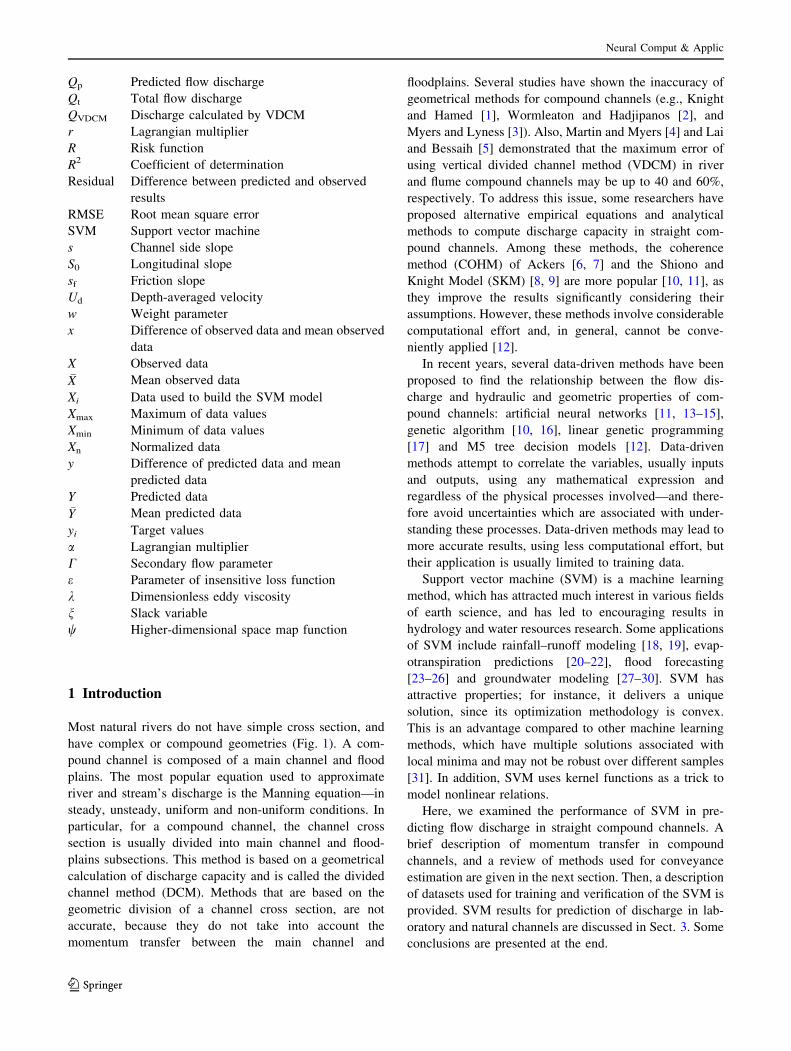
Qp Predicted flow discharge

Qt Total flow discharge

QVDCM Discharge calculated by VDCM

r Lagrangian multiplier

R Risk function

R2 Coefficient of determination

Residual Difference between predicted and observed

results

RMSE Root mean square error

SVM Support vector machine

s Channel side slope

S0 Longitudinal slope

sf Friction slope

Ud Depth-averaged velocity

w Weight parameter

x Difference of observed data and mean observed

data

X Observed data�X Mean observed data

Xi Data used to build the SVM model

Xmax Maximum of data values

Xmin Minimum of data values

Xn Normalized data

y Difference of predicted data and mean

predicted data

Y Predicted data�Y Mean predicted data

yi Target values

a Lagrangian multiplier

C Secondary flow parameter

e Parameter of insensitive loss function

k Dimensionless eddy viscosity

n Slack variable

w Higher-dimensional space map function

1 Introduction

Most natural rivers do not have simple cross section, and

have complex or compound geometries (Fig. 1). A com-

pound channel is composed of a main channel and flood

plains. The most popular equation used to approximate

river and stream’s discharge is the Manning equation—in

steady, unsteady, uniform and non-uniform conditions. In

particular, for a compound channel, the channel cross

section is usually divided into main channel and flood-

plains subsections. This method is based on a geometrical

calculation of discharge capacity and is called the divided

channel method (DCM). Methods that are based on the

geometric division of a channel cross section, are not

accurate, because they do not take into account the

momentum transfer between the main channel and

floodplains. Several studies have shown the inaccuracy of

geometrical methods for compound channels (e.g., Knight

and Hamed [1], Wormleaton and Hadjipanos [2], and

Myers and Lyness [3]). Also, Martin and Myers [4] and Lai

and Bessaih [5] demonstrated that the maximum error of

using vertical divided channel method (VDCM) in river

and flume compound channels may be up to 40 and 60%,

respectively. To address this issue, some researchers have

proposed alternative empirical equations and analytical

methods to compute discharge capacity in straight com-

pound channels. Among these methods, the coherence

method (COHM) of Ackers [6, 7] and the Shiono and

Knight Model (SKM) [8, 9] are more popular [10, 11], as

they improve the results significantly considering their

assumptions. However, these methods involve considerable

computational effort and, in general, cannot be conve-

niently applied [12].

In recent years, several data-driven methods have been

proposed to find the relationship between the flow dis-

charge and hydraulic and geometric properties of com-

pound channels: artificial neural networks [11, 13–15],

genetic algorithm [10, 16], linear genetic programming

[17] and M5 tree decision models [12]. Data-driven

methods attempt to correlate the variables, usually inputs

and outputs, using any mathematical expression and

regardless of the physical processes involved—and there-

fore avoid uncertainties which are associated with under-

standing these processes. Data-driven methods may lead to

more accurate results, using less computational effort, but

their application is usually limited to training data.

Support vector machine (SVM) is a machine learning

method, which has attracted much interest in various fields

of earth science, and has led to encouraging results in

hydrology and water resources research. Some applications

of SVM include rainfall–runoff modeling [18, 19], evap-

otranspiration predictions [20–22], flood forecasting

[23–26] and groundwater modeling [27–30]. SVM has

attractive properties; for instance, it delivers a unique

solution, since its optimization methodology is convex.

This is an advantage compared to other machine learning

methods, which have multiple solutions associated with

local minima and may not be robust over different samples

[31]. In addition, SVM uses kernel functions as a trick to

model nonlinear relations.

Here, we examined the performance of SVM in pre-

dicting flow discharge in straight compound channels. A

brief description of momentum transfer in compound

channels, and a review of methods used for conveyance

estimation are given in the next section. Then, a description

of datasets used for training and verification of the SVM is

provided. SVM results for prediction of discharge in lab-

oratory and natural channels are discussed in Sect. 3. Some

conclusions are presented at the end.

Neural Comput & Applic

123

2 Methods

2.1 Momentum transfer in compound channels

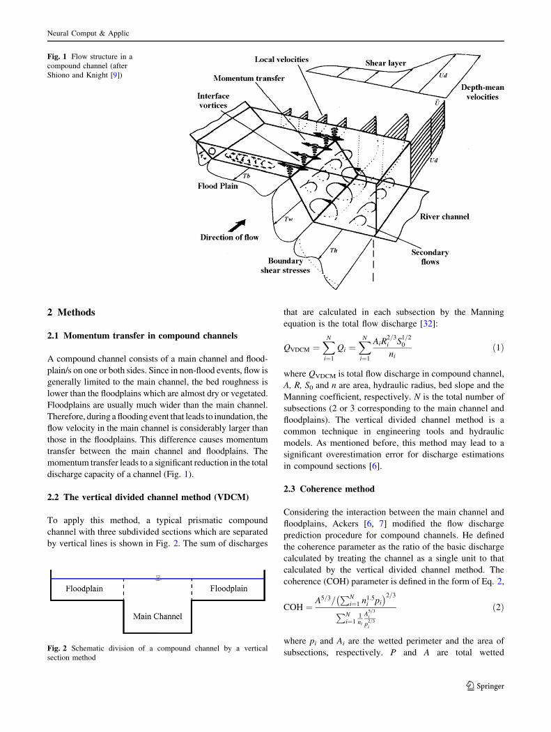
A compound channel consists of a main channel and flood-

plain/s on one or both sides. Since in non-flood events, flow is

generally limited to the main channel, the bed roughness is

lower than the floodplains which are almost dry or vegetated.

Floodplains are usually much wider than the main channel.

Therefore, during a flooding event that leads to inundation, the

flow velocity in the main channel is considerably larger than

those in the floodplains. This difference causes momentum

transfer between the main channel and floodplains. The

momentum transfer leads to a significant reduction in the total

discharge capacity of a channel (Fig. 1).

2.2 The vertical divided channel method (VDCM)

To apply this method, a typical prismatic compound

channel with three subdivided sections which are separated

by vertical lines is shown in Fig. 2. The sum of discharges

that are calculated in each subsection by the Manning

equation is the total flow discharge [32]:

QVDCM ¼XN

i¼1

Qi ¼XN

i¼1

AiR2=3i S

1=20

nið1Þ

where QVDCM is total flow discharge in compound channel,

A, R, S0 and n are area, hydraulic radius, bed slope and the

Manning coefficient, respectively. N is the total number of

subsections (2 or 3 corresponding to the main channel and

floodplains). The vertical divided channel method is a

common technique in engineering tools and hydraulic

models. As mentioned before, this method may lead to a

significant overestimation error for discharge estimations

in compound sections [6].

2.3 Coherence method

Considering the interaction between the main channel and

floodplains, Ackers [6, 7] modified the flow discharge

prediction procedure for compound channels. He defined

the coherence parameter as the ratio of the basic discharge

calculated by treating the channel as a single unit to that

calculated by the vertical divided channel method. The

coherence (COH) parameter is defined in the form of Eq. 2,

COH ¼A5=3=

PNi¼1 n

1:5i pi

� �2=3

PNi¼1

1ni

A5=3i

p2=3i

ð2Þ

where pi and Ai are the wetted perimeter and the area of

subsections, respectively. P and A are total wetted

Fig. 1 Flow structure in a

compound channel (after

Shiono and Knight [9])

Fig. 2 Schematic division of a compound channel by a vertical

section method

Neural Comput & Applic

123

perimeter and area of the channel. Alternatively, Eq. (3)

can be used more conveniently to compute COH,

COH ¼1þ A�ð Þ3=2=

ffiffiffiffiffiffiffiffiffiffiffiffiffiffiffiffiffiffiffiffiffiffiffi1þ P

�43n�2

A�13

� �r

1þ A�5=3=n�P�2=3 ð3Þ

The star (*) symbol represents the ratio of a parameter

value in the floodplain to that in the main channel. A COH

close to 1 indicated that a compound channel can be accu-

rately treated as a simple channel. As COH deviated from 1,

this approximation leads to errors. By analyzing the smooth

compound channel data of flood channel facility (FCF),

Ackers [6, 7] suggested different degrees of interference

between the main channel and floodplain flow according to

the relative depth (ratio of water depth in floodplain to that in

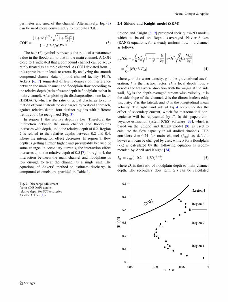
main channel). After plotting the discharge adjustment factor

(DISDAF), which is the ratio of actual discharge to sum-

mation of zonal calculated discharges by vertical approach,

against relative depth, four distinct regions with different

trends could be recognized (Fig. 3).

In region 1, the relative depth is low. Therefore, the

interaction between the main channel and floodplains

increases with depth, up to the relative depth of 0.2. Region

2 is related to the relative depths between 0.2 and 0.4,

where the interaction effect decreases. In region 3, flow

depth is getting further higher and presumably because of

some changes in secondary currents, the interaction effect

increases up to the relative depth of 0.5 [7]. In region 4, the

interaction between the main channel and floodplains is

low enough to treat the channel as a single unit. The

equations of Ackers’ method to estimate discharge in

compound channels are provided in Table 1.

2.4 Shiono and Knight model (SKM)

Shiono and Knight [8, 9] presented their quasi-2D model,

which is based on Reynolds-averaged Navier–Stokes

(RANS) equations, for a steady uniform flow in a channel

as follows,

qgHS0 � qf

8U2

d

ffiffiffiffiffiffiffiffiffiffiffiffi1þ 1

s2

rþ o

oyqkH2

ffiffiffif

8

rUd

oUd

oy

" #

¼ o

oyH qUVð Þd� �

ð4Þ

where q is the water density, g is the gravitational accel-

eration, f is the friction factor, H is local depth flow, y

denotes the transverse direction with the origin at the side

wall, Ud is the depth-averaged stream-wise velocity, s is

the side slope of the channel, k is the dimensionless eddy

viscosity, V is the lateral, and U is the longitudinal mean

velocity. The right hand side of Eq. 4 accommodates the

effect of secondary current, which for mathematical con-

venience will be represented by C. In this paper, con-

veyance estimation system (CES) software [33], which is

based on the Shiono and Knight model [9], is used to

calculate the flow capacity in all studied channels. CES

considers k = 0.24 for main channel (kmc) as default;

however, it can be changed by user, while k for a floodplain(kfp) is calculated by the following equation as recom-

mended by Abril and Knight [34]:

kfp ¼ kmc �0:2þ 1:2D�1:44r

� �ð5Þ

where Dr is the ratio of floodplain depth to main channel

depth. The secondary flow term (C) can be calculated

Fig. 3 Discharge adjustment

factor (DISDAF) against

relative depth for FCF test series

2 (after Ackers [7])

Neural Comput & Applic

123

depending on the water level in the channel (inbank,

overbank, flood plain scenarios) which is recommended by

Abril and Knight [34] as follows:

Cmci ¼ 0:05HqgS0 ð6ÞCmco ¼ 0:15HqgS0 ð7ÞCfp ¼ �0:25HqgS0 ð8Þ

where Cmci, Cmco and Cfp are secondary current parameters

for main channel inbank, overbank and floodplain scenar-

ios, respectively.

2.5 Support vector machines

Support vector machine (SVM) is a learning machine

method developed by Vapnik and his colleagues [35, 36].

Initial applications of support vector machine included

classification and pattern recognition [37]. Excellent per-

formance of SVM was reported in regression and time-

series analysis applications [38]. The basic idea of SVM is

to map the training data from the input space to a higher-

dimensional feature space via a kernel function u and then

to construct a hyperplane with maximum margin in the

feature space. Therefore, SVM uses linear functions in a

higher-dimensional space to classify linearly, for classifi-

cation purposes and interpolate a set of training data lin-

early, for regression purposes. In this study, the e-SVMmethod [39] was used to construct an input–output model.

Considering a set of training data as

x1; y1ð Þ; x2; y2ð Þ; . . . xl; ylð Þf g � v� R, where v denotes the

space of input patterns. The linear function in space of x

could be described as follows,

f xð Þ ¼ w � xþ b ð9Þ

where w is the weight and b is the bias term, which are

estimated by minimizing the following risk function,

R ¼ C1

l

XN

i¼1

Le yi; fið Þ þ 1

2wk k2 ð10Þ

where C is constant called penalty and Le is loss function

described in Eq. (11), yi and fi are actual target values and

estimated target values by Eq. (9), respectively.

Le yi; fið Þ ¼ 0 if yi � fij j � eyi � fij j � e otherwise

ð11Þ

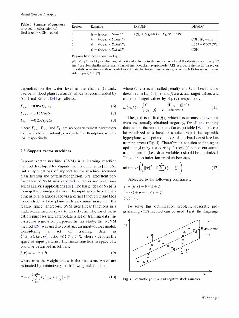
The goal is to find f(x) which has at most e deviation

from the actually obtained targets yi for all the training

data, and at the same time as flat as possible [39]. This can

be visualized as a band or a tube around the separable

hyperplane with points outside of the band considered as

training errors (Fig. 4). Therefore, in addition to finding an

optimum f(x) by considering flatness (function curvature)

training errors (i.e., slack variables) should be minimized.

Thus, the optimization problem becomes,

minimize1

2wk k2þC

Xn

i¼1

ni þ n�i� �

!ð12Þ

Subjected to the following constraints,

yi � w:xð Þ � b� eþ niw � xð Þ þ b� yi � eþ n�ini; n

�i � 0

To solve this optimization problem, quadratic pro-

gramming (QP) method can be used. First, the Lagrange

Fig. 4 Schematic positive and negative slack variables

Table 1 Summary of equations

involved in calculation of

discharge by COH method

Region Equation DISDEF DISADF

1 Q ¼ QVDCM � DISDEF ðQ�2c þ NfQ

�2fÞ Vc � Vfð ÞHh� ARF

2 Q ¼ QVDCM � DISADF2 COH Dr þ shift½ ð Þ3 Q ¼ QVDCM � DISADF3 1:567� 0:667COH

4 Q ¼ QVDCM � DISADF4 COH

Regions have been shown in Fig. 3

Q�2c, Vc, Q

�2f and Vf are discharge deficit and velocity in the main channel and floodplain, respectively. H

and h are flow depths in the main channel and floodplain, respectively. ARF is aspect ratio factor. In region

2, a shift in relative depth is needed to estimate discharge more accurate, which is 0.15 for main channel

side slope sc � 1 [7]

Neural Comput & Applic

123

function, which contains target function with its subjects, is

formed.

L ¼ 1

2wk k2þC

Xn

i¼1

ni þ n�i� �

�Xn

i¼1

ai wi � xþ bð Þ � yi þ eþ nið Þ½

�Xn

i¼1

a�i yi � wi � xþ bð Þ þ eþ n�i� �� �

�Xn

i¼1

rini þ r�i n�i

� �

ð13Þ

where ai, a�i , ri and r�i are Lagrange multipliers and for

any data they are nonnegative. Equation (13) is mini-

mized with respect to variables w, b, n and n* and is

maximized with respect to Lagrange multipliers a, a*, rand r*. After differentiating with respect to these param-

eters and setting the derivatives to zero, Eqs. (14)–(17)

are obtained.

oL

ow¼ 0 ! w ¼

XN

i¼1

ai � a�i� �

xi ð14Þ

oL

ob¼ 0 !

XN

i¼1

ai � a�i� �

¼ 0 ð15Þ

oL

oni¼ 0 ! C ¼ ai þ ri ð16Þ

oL

on�i¼ 0 ! C ¼ a�i þ r�i ð17Þ

By substituting these equations into Eq. (13), a dual

Lagrangian function dependent only on a is obtained,

which requires to be maximized.

max D að Þð Þ ¼ maxX

ai � a�i� �

yi � eX

ai � a�i� ��

� 1

2

XN

i¼1

XN

j¼1

ai � a�i� �

aj � a�j

� �Kðxi; xjÞ

!

ð18Þ

subjected to the following constraints,

Xai � a�i� �

¼ 0 0� ai �C 0� a�i �C

where K(xi, xj) is the kernel function.

Kernel function is a method to handle input spaces,

which are not linear in the space of x, but can linearly be

regressed in a higher-dimensional space of w(x). Therefore,the kernel function job is to map x to w(x). In order to use

the kernel method, in previous equations, w(x) substitutesfor x. The kernel function is,

K xi; xj� �

¼ wðxiÞ � w xj� �

ð19Þ

The SVM regression function modeling the data after

modifying Eq. (9) by considering Eqs. (18) and (19) can be

written as follows,

f ¼XN

i¼1

ai � a�i� �

K xi; xj� �

þ b ð20Þ

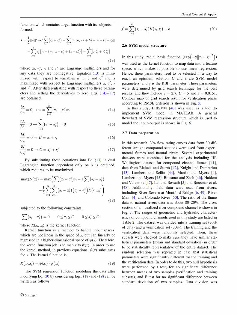
2.6 SVM model structure

In this study, radial basis function (exp �c xi � xj 2

� �)

was used as the kernel function to map data into a feature

space, which makes it possible to use linear regression.

Hence, three parameters need to be selected in a way to

reach an optimum solution. C and e are SVM model

parameters, and c is the RBF parameter. These parameters

were determined by grid search technique for the best

results, and they include c = 2.7, C = 5 and e = 0.0151.

Contour map of grid search result for verification phase

according to RMSE criterion is shown in Fig. 5.

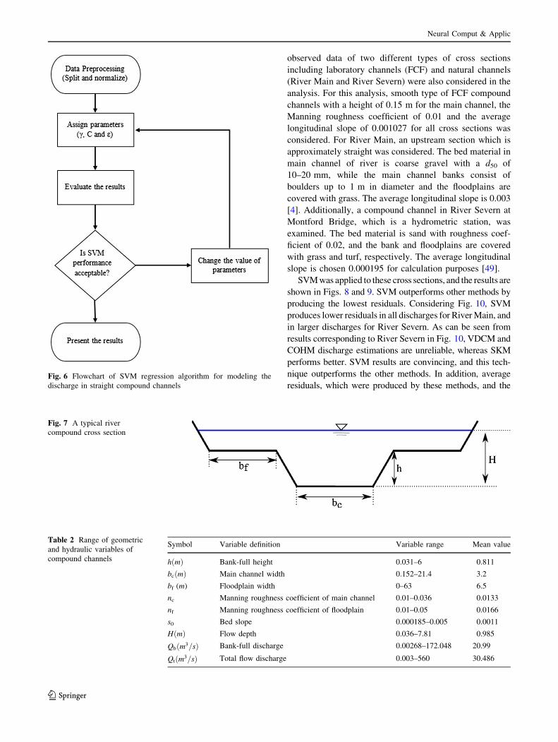
In this study, LIBSVM [40] was used as a tool to

implement SVM model in MATLAB. A general

flowchart of SVM regression structure which is used to

model the input–output is shown in Fig. 6.

2.7 Data preparation

In this research, 394 flow rating curves data from 30 dif-

ferent straight compound sections were used from experi-

mental flumes and natural rivers. Several experimental

datasets were combined for the analysis including HR

Wallingford dataset for compound channel flumes [41],

data from Blalock and Sturm [42], Knight and Demetriou

[43], Lambert and Sellin [44], Martin and Myers [4],

Lambert and Myers [45], Bousmar and Zech [46], Haidera

and Valentine [47], Lai and Bessaih [5] and Bousmar et al.

[48]. Additionally, field data were used from rivers,

including River Severn at Montford Bridge [6, 49], River

Main [4] and Colorado River [50]. The ratio of the flume

data to natural rivers data was about 80–20%. The cross

section of an idealized river compound channel is shown in

Fig. 7. The ranges of geometric and hydraulic character-

istics of compound channels used in this study are listed in

Table 2. The dataset was divided into a training set (70%

of data) and a verification set (30%). The training and the

verification data were randomly selected. Then, these

subsets were checked to make sure they have similar sta-

tistical parameters (mean and standard deviation) in order

to be statistically representative of the entire dataset. The

random selection was repeated in case that statistical

parameters were significantly different for the training and

the verification data. In order to do this, two null hypothesis

were performed by t test, for no significant difference

between means of two samples (verification and training

subsets), and F test for no significant difference between

standard deviation of two samples. Data division was

Neural Comput & Applic

123

performed in a way that these hypotheses would be

accepted in a significance level of 0.05.

Since a wide range of data with different scales were

used, with the application of Eq. (21), input data are first

normalized to a range between 0 and 1. The normalization

helps to speed up the model convergence. The data are

normalized using the folllowing equation,

Xn ¼Xi � Xmin

Xmax � Xmin

ð21Þ

where Xn is the normalized data, Xi is the raw data, and

Xmin and Xmax are the minimum and maximum of data.

In this paper, it is assumed (similar to Ackers [6, 7]

approach) that discharge ratio in compound open channels

is dependent on three input dimensionless parameters,

including relative depth, Dr, coherence parameter, COH,

and calculated discharge ratio (QVDCM

Qb).

Qt

Qb

¼ f Dr;COH;QVDCM

Qb

� �ð22Þ

where Qt and Qb are total and bank-full flow discharges,

respectively.

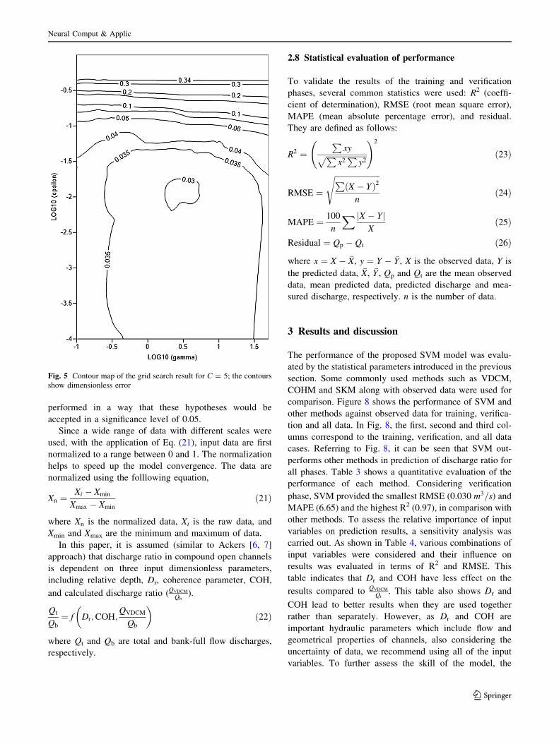
2.8 Statistical evaluation of performance

To validate the results of the training and verification

phases, several common statistics were used: R2 (coeffi-

cient of determination), RMSE (root mean square error),

MAPE (mean absolute percentage error), and residual.

They are defined as follows:

R2 ¼P

xyffiffiffiffiffiffiffiffiffiffiffiffiffiffiffiffiffiffiffiffiffiPx2P

y2p

!2

ð23Þ

RMSE ¼

ffiffiffiffiffiffiffiffiffiffiffiffiffiffiffiffiffiffiffiffiffiffiffiPX � Yð Þ2

n

s

ð24Þ

MAPE ¼ 100

n

X X � Yj jX

ð25Þ

Residual ¼ Qp � Qt ð26Þ

where x ¼ X � �X, y ¼ Y � �Y , X is the observed data, Y is

the predicted data, �X, �Y , Qp and Qt are the mean observed

data, mean predicted data, predicted discharge and mea-

sured discharge, respectively. n is the number of data.

3 Results and discussion

The performance of the proposed SVM model was evalu-

ated by the statistical parameters introduced in the previous

section. Some commonly used methods such as VDCM,

COHM and SKM along with observed data were used for

comparison. Figure 8 shows the performance of SVM and

other methods against observed data for training, verifica-

tion and all data. In Fig. 8, the first, second and third col-

umns correspond to the training, verification, and all data

cases. Referring to Fig. 8, it can be seen that SVM out-

performs other methods in prediction of discharge ratio for

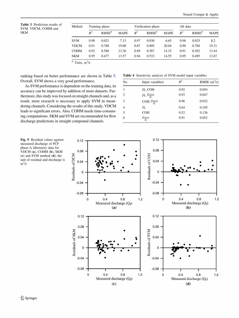
all phases. Table 3 shows a quantitative evaluation of the

performance of each method. Considering verification

phase, SVM provided the smallest RMSE (0.030 m3=s) and

MAPE (6.65) and the highest R2 (0.97), in comparison with

other methods. To assess the relative importance of input

variables on prediction results, a sensitivity analysis was

carried out. As shown in Table 4, various combinations of

input variables were considered and their influence on

results was evaluated in terms of R2 and RMSE. This

table indicates that Dr and COH have less effect on the

results compared to QVDCM

Qt. This table also shows Dr and

COH lead to better results when they are used together

rather than separately. However, as Dr and COH are

important hydraulic parameters which include flow and

geometrical properties of channels, also considering the

uncertainty of data, we recommend using all of the input

variables. To further assess the skill of the model, the

Fig. 5 Contour map of the grid search result for C = 5; the contours

show dimensionless error

Neural Comput & Applic

123

observed data of two different types of cross sections

including laboratory channels (FCF) and natural channels

(River Main and River Severn) were also considered in the

analysis. For this analysis, smooth type of FCF compound

channels with a height of 0.15 m for the main channel, the

Manning roughness coefficient of 0.01 and the average

longitudinal slope of 0.001027 for all cross sections was

considered. For River Main, an upstream section which is

approximately straight was considered. The bed material in

main channel of river is coarse gravel with a d50 of

10–20 mm, while the main channel banks consist of

boulders up to 1 m in diameter and the floodplains are

covered with grass. The average longitudinal slope is 0.003

[4]. Additionally, a compound channel in River Severn at

Montford Bridge, which is a hydrometric station, was

examined. The bed material is sand with roughness coef-

ficient of 0.02, and the bank and floodplains are covered

with grass and turf, respectively. The average longitudinal

slope is chosen 0.000195 for calculation purposes [49].

SVMwas applied to these cross sections, and the results are

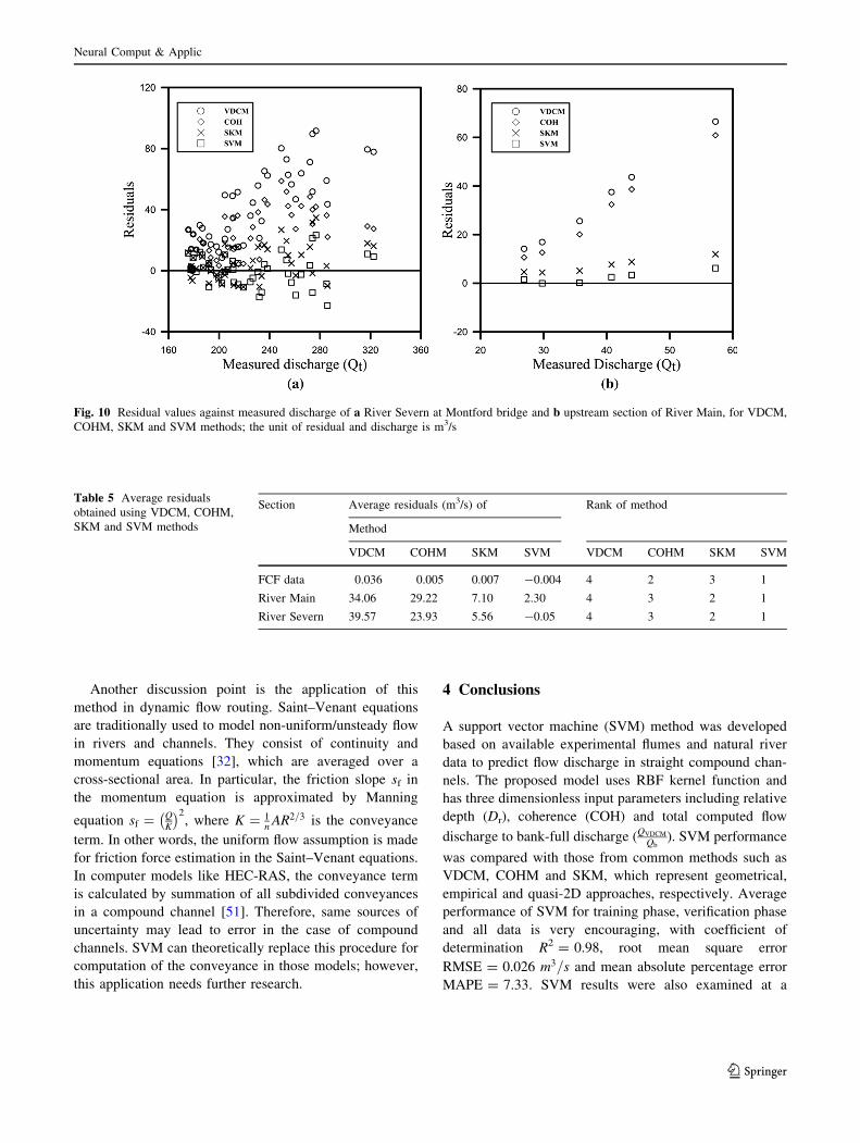
shown in Figs. 8 and 9. SVM outperforms other methods by

producing the lowest residuals. Considering Fig. 10, SVM

produces lower residuals in all discharges for RiverMain, and

in larger discharges for River Severn. As can be seen from

results corresponding to River Severn in Fig. 10, VDCM and

COHM discharge estimations are unreliable, whereas SKM

performs better. SVM results are convincing, and this tech-

nique outperforms the other methods. In addition, average

residuals, which were produced by these methods, and the

Fig. 7 A typical river

compound cross section

Table 2 Range of geometric

and hydraulic variables of

compound channels

Symbol Variable definition Variable range Mean value

h mð Þ Bank-full height 0.031–6 0.811

bc mð Þ Main channel width 0.152–21.4 3.2

bf (m) Floodplain width 0–63 6.5

nc Manning roughness coefficient of main channel 0.01–0.036 0.0133

nf Manning roughness coefficient of floodplain 0.01–0.05 0.0166

s0 Bed slope 0.000185–0.005 0.0011

H mð Þ Flow depth 0.036–7.81 0.985

Qb m3=sð Þ Bank-full discharge 0.00268–172.048 20.99

Qt m3=sð Þ Total flow discharge 0.003–560 30.486

Fig. 6 Flowchart of SVM regression algorithm for modeling the

discharge in straight compound channels

Neural Comput & Applic

123

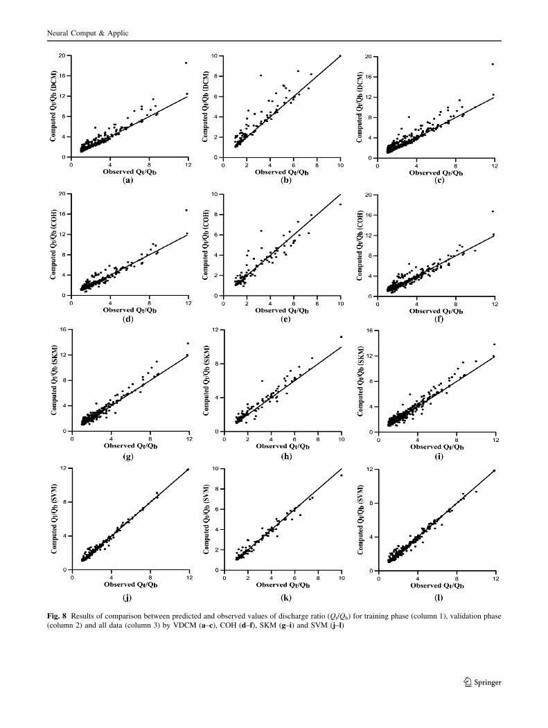
Fig. 8 Results of comparison between predicted and observed values of discharge ratio (Qt/Qb) for training phase (column 1), validation phase

(column 2) and all data (column 3) by VDCM (a–c), COH (d–f), SKM (g–i) and SVM (j–l)

Neural Comput & Applic

123

ranking based on better performance are shown in Table 5.

Overall, SVM shows a very good performance.

As SVM performance is dependent on the training data, its

accuracy can be improved by addition of more datasets. Fur-

thermore, this studywas focused on straight channels and, as a

result, more research is necessary to apply SVM in mean-

dering channels. Considering the results of this study, VDCM

leads to significant errors. Also, COHM needs time-consum-

ing computations. SKM and SVM are recommended for flow

discharge predictions in straight compound channels.

Table 3 Prediction results of

SVM, VDCM, COHM and

SKM

Method Training phase Verification phase All data

R2 RMSE# MAPE R2 RMSE# MAPE R2 RMSE# MAPE

SVM 0.98 0.023 7.13 0.97 0.030 6.65 0.98 0.025 8.2

VDCM 0.91 0.780 19.00 0.87 0.805 20.04 0.90 0.788 19.31

COHM 0.92 0.580 13.30 0.89 0.587 14.15 0.91 0.582 13.44

SKM 0.95 0.477 13.57 0.94 0.533 14.55 0.95 0.495 13.87

# Units, m3/s

Table 4 Sensitivity analysis of SVM model input variables

No Input variable/s R2 RMSE (m3/s)

1 Dr;COH 0.92 0.054

2 Dr;QVDCM

Qt

0.93 0.047

3 COH; QVDCM

Qt

0.96 0.032

4 Dr 0.64 0.105

5 COH 0.52 0.126

6 QVDCM

Qt

0.91 0.052

Fig. 9 Residual values against

measured discharge of FCF

phase-A laboratory data for

VDCM (a), COHM (b), SKM(c) and SVM method (d); theunit of residual and discharge is

m3/s

Neural Comput & Applic

123

Another discussion point is the application of this

method in dynamic flow routing. Saint–Venant equations

are traditionally used to model non-uniform/unsteady flow

in rivers and channels. They consist of continuity and

momentum equations [32], which are averaged over a

cross-sectional area. In particular, the friction slope sf in

the momentum equation is approximated by Manning

equation sf ¼ QK

� �2, where K ¼ 1

nAR2=3 is the conveyance

term. In other words, the uniform flow assumption is made

for friction force estimation in the Saint–Venant equations.

In computer models like HEC-RAS, the conveyance term

is calculated by summation of all subdivided conveyances

in a compound channel [51]. Therefore, same sources of

uncertainty may lead to error in the case of compound

channels. SVM can theoretically replace this procedure for

computation of the conveyance in those models; however,

this application needs further research.

4 Conclusions

A support vector machine (SVM) method was developed

based on available experimental flumes and natural river

data to predict flow discharge in straight compound chan-

nels. The proposed model uses RBF kernel function and

has three dimensionless input parameters including relative

depth (Dr), coherence (COH) and total computed flow

discharge to bank-full discharge (QVDCM

Qb). SVM performance

was compared with those from common methods such as

VDCM, COHM and SKM, which represent geometrical,

empirical and quasi-2D approaches, respectively. Average

performance of SVM for training phase, verification phase

and all data is very encouraging, with coefficient of

determination R2 = 0.98, root mean square error

RMSE = 0.026 m3=s and mean absolute percentage error

MAPE = 7.33. SVM results were also examined at a

Fig. 10 Residual values against measured discharge of a River Severn at Montford bridge and b upstream section of River Main, for VDCM,

COHM, SKM and SVM methods; the unit of residual and discharge is m3/s

Table 5 Average residuals

obtained using VDCM, COHM,

SKM and SVM methods

Section Average residuals (m3/s) of Rank of method

Method

VDCM COHM SKM SVM VDCM COHM SKM SVM

FCF data 0.036 0.005 0.007 -0.004 4 2 3 1

River Main 34.06 29.22 7.10 2.30 4 3 2 1

River Severn 39.57 23.93 5.56 -0.05 4 3 2 1

Neural Comput & Applic

123

number of cross sections in River Main and River Severn.

SVM outperforms other methods in predicting flow dis-

charge with average residual of -0.004, 2.30 and -0.05

for FCF flumes, River Main and River Severn, respec-

tively. SVM’s satisfactory results indicated that it can be

applied as a reliable technique for the prediction of flow

discharge in straight compound channels. The method can

be incorporated into numerical river models with further

research.

Compliance with ethical standards

Conflict of interest The authors declare that they have no conflict of

interest.

References

1. Knight DW, Hamed ME (1984) Boundary shear in symmetrical

compound channels. J Hydraul Eng 110(10):1412–1430

2. Wormleaton PR, Hadjipanos P (1985) Flow distribution in

compound channels. J Hydraul Eng 111(2):357–361

3. Myers R, Lyness J (1997) Discharge ratios in smooth and rough

compound channels. J Hydraul Eng 123(3):182–188

4. Martin L, Myers W (1991) Measurement of overbank flow in a

compound river channel. ICE Proc 91(4):645–657

5. Lai S, Bessaih N (2004) Flow in compound channels. In: 1st

International conference on managing rivers in the 21st century,

Malaysia, pp 275–280

6. Ackers P (1992) Hydraulic design of two-stage channels. Proc

ICE-Water Marit Energy 96(4):247–257

7. Ackers P (1993) Flow formulae for straight two-stage channels.

J Hydraul Res 31(4):509–531

8. Shiono K, Knight D (1988) Two-dimensional analytical solution

for a compound channel. In: Proceedings of 3rd international

symposium on refined flow modelling and turbulence measure-

ments, pp 503–510

9. Shiono K, Knight DW (1991) Turbulent open-channel flows with

variable depth across the channel. J Fluid Mech 222:617–646

10. Sharifi S, Sterling M, Knight DW (2009) A novel application of a

multi-objective evolutionary algorithm in open channel flow

modelling. J Hydroinform 11(1):31. doi:10.2166/hydro.2009.033

11. Unal B, Mamak M, Seckin G, Cobaner M (2010) Comparison of

an ANN approach with 1-D and 2-D methods for estimating

discharge capacity of straight compound channels. Adv Eng

Softw 41(2):120–129. doi:10.1016/j.advengsoft.2009.10.002

12. Zahiri A, Azamathulla HM (2012) Comparison between linear

genetic programming and M5 tree models to predict flow dis-

charge in compound channels. Neural Comput Appl

24(2):413–420. doi:10.1007/s00521-012-1247-0

13. MacLeod AB (1997) Development of methods to predict the

discharge capacity in model and prototype meandering compound

channels. University of Glasgow

14. Liu W, James C (2000) Estimation of discharge capacity in

meandering compound channels using artificial neural networks.

Can J Civ Eng 27(2):297–308

15. Zahiri A, Dehghani A (2009) Flow discharge determination in

straight compound channels using ANN. World Acad Sci Eng

Technol 58:1–8

16. Sharifi S (2009) Application of evolutionary computation to open

channel flow modelling. University of Birmingham, Birmingham,

UK

17. Azamathulla HM, Zahiri A (2012) Flow discharge prediction in

compound channels using linear genetic programming. J Hydrol

454–455:203–207

18. Dibike YB, Velickov S, Solomatine D, Abbott MB (2001) Model

induction with support vector machines: introduction and appli-

cations. J Comput Civ Eng

19. Bray M, Han D (2004) Identification of support vector machines

for runoff modelling. J Hydroinform 6:265–280

20. Eslamian S, Gohari S, Biabanaki M, Malekian R (2008) Esti-

mation of monthly pan evaporation using artificial neural net-

works and support vector machines. J Appl Sci 8(19):3497–3502

21. Samui P (2011) Application of least square support vector

machine (LSSVM) for determination of evaporation losses in

reservoirs. Engineering 3(04):431

22. Tabari H, Kisi O, Ezani A, Talaee PH (2012) SVM, ANFIS,

regression and climate based models for reference evapotran-

spiration modeling using limited climatic data in a semi-arid

highland environment. J Hydrol 444:78–89

23. Han D, Chan L, Zhu N (2007) Flood forecasting using support

vector machines. J Hydroinform 9(4):267–276

24. Chen S-T, Yu P-S (2007) Pruning of support vector networks on

flood forecasting. J Hydrol 347(1):67–78

25. Yu P-S, Chen S-T, Chang I-F (2006) Support vector regression

for real-time flood stage forecasting. J Hydrol 328(3):704–716

26. Hashemi MR, Spaulding ML, Shaw A, Farhadi H, Lewis M

(2016) An efficient artificial intelligence model for prediction of

tropical storm surge. Nat Hazards 82(1):471–491

27. Behzad M, Asghari K, Coppola EA Jr (2009) Comparative study

of SVMs and ANNs in aquifer water level prediction. J Comput

Civ Eng 24(5):408–413

28. Yoon H, Jun S-C, Hyun Y, Bae G-O, Lee K-K (2011) A com-

parative study of artificial neural networks and support vector

machines for predicting groundwater levels in a coastal aquifer.

J Hydrol 396(1):128–138

29. Liu J, Chang J-X, Zhang W-G (2009) Groundwater level dynamic

prediction based on chaos optimization and support vector

machine. In: Genetic and evolutionary computing, 2009.

WGEC’09. 3rd International Conference on. IEEE, pp 39–43

30. Liu J, Chang M, Ma X (2009) Groundwater quality assessment

based on support vector machine. In: HAIHE river basin research

and planning approach-proceedings of 2009 international sym-

posium of HAIHE basin integrated water and environment

management, pp 173–178

31. Auria L, Moro RA (2008) Support vector machines (SVM) as a

technique for solvency analysis. German Institute for Economic

Research, Berlin, Germany

32. Chow VT (1959) Open-channel hydraulic. McGraw-Hill, New

York

33. McGahey C, Samuels P (2003) Methodology for conveyance

estimation in two-stage straight, skewed and meandering chan-

nels. In: Proceedings of the XXX congress of the international

association for hydraulic research, pp 33–40

34. Abril J, Knight D (2004) Stage-discharge prediction for rivers in

flood applying a depth-averaged model. J Hydraul Res

42(6):616–629

35. Vapnik V (1995) The nature of statistical learning theory.

Springer, Berlin

36. Cortes C, Vapnik V (1995) Support-vector networks. Mach Learn

20(3):273–297

37. Scholkopf B, Burges C, Vapnik V (1995) Extracting support data

for a given task. In: KDD

38. Mattera D, Haykin S (1999) Support vector machines for

dynamic reconstruction of a chaotic system. In: Advances in

kernel methods. MIT Press, Cambridge, pp 211–241

39. Smola AJ, Scholkopf B (2004) A tutorial on support vector

regression. Stat Comput 14(3):199–222

Neural Comput & Applic

123

40. Chang C-C, Lin C-J (2011) LIBSVM: a library for support vector

machines. ACM Trans Intell Syst Technol 2(3):27

41. Knight D, Sellin R (1987) The SERC flood channel facility.

Water Environ J 1(2):198–204

42. Blalock ME, Sturm TW (1981) Minimum specific energy in

compound open channel. J Hydraul Div 107(6):699–717

43. Knight DW, Demetriou JD (1983) Flood plain and main channel

flow interaction. J Hydraul Eng 109(8):1073–1092

44. Lambert M, Sellin R (1996) Discharge prediction in straight

compound channels using the mixing length concept. J Hydraul

Res 34(3):381–394

45. Lambert MF, Myers W (1998) Estimating the discharge capacity

in straight compound channels. Proc ICE-Water Marit Energy

130(2):84–94

46. Bousmar D, Zech Y (1999) Momentum transfer for practical flow

computation in compound channels. J Hydraul Eng

125(7):696–706

47. Haidera M, Valentine E (2002) A practical method for predicting

the total discharge in mobile and rigid boundary compound

channels. In: International conference on fluvial hydraulics,

Belgium. pp 153–160

48. Bousmar D, Wilkin N, Jacquemart J-H, Zech Y (2004) Overbank

flow in symmetrically narrowing floodplains. J Hydraul Eng

130(4):305–312

49. Knight D, Shiono K, Pirt J (1989) Prediction of depth mean

velocity and discharge in natural rivers with overbank flow. In:

Proceedings of the international conference on hydraulic and

environmental modelling of Coastal, Estuarine and River Waters,

pp 419–428

50. Tarrab L, Weber J (2004) Prediccion del coeficiente de mezcla

transversal en cauces aturales. Mecanica Computacional, XXIII,

Asociacion Argentina de Mecanica Computacional, San Carlos

de Bariloche, pp 1343–1355

51. Brunner GW CEIWR-HEC (2010) HEC-RAS river analysis

system user’s manual version 4.1. In: Tech. Rep., US Army Corps

of Engineers Institute for Water Resources Hydrologic Engi-

neering Center (HEC), CA, USA

Neural Comput & Applic

123