Income Guarantees and Borrowing in

Risky Environments. Evidence from

India’s Rural Employment Guarantee

Scheme ∗

Clive Bell a, b and Abhiroop Mukhopadhyay c

a University of Heidelberg, INF 330, D-69120 Heidelberg, Germany

b Chr. Michelsen Institute, P.O. Box 6033, N-5892 Bergen, Norway

c Indian Statistical Institute, Delhi, 110016, India

clive.bell@urz.uni-heidelberg.de abhiroop@isid.ac.in

First version: 27.06.2013. This version: 14.09.2015

∗Earlier versions of this paper were presented at CMI and the Delhi School of Economics. We are

particularly indebted to Magnus Hatlebakk for numerous and valuable discussions. All responsibility

for any remaining errors of formulation and analysis is ours alone.

1

Abstract

This paper investigates the effects of an income guarantee on borrowing to

smooth consumption and finance cultivation in a risky setting with marked

seasonality. A three-season, infinite-horizon theoretical model is developed

and analyzed, and certain of its results are tested empirically on a sample of

households in a semi-arid region of Odisha state, with reference to India’s

National Rural Employment Guarantee Scheme (NREGS). The potential

endogeneity of borrowing and NREGS earnings is instrumented using the

female reservation for local elections. An additional day of work at the

regulated wage reduces the estimated amount borrowed for consumption

by about half the wage. For the financing of working capital, it increases

such borrowing by an estimated amount that is almost twice as large as

the wage. NREGS is therefore effectively a substitute for borrowing if a

household does not cultivate, but a complement if it does so.

Keywords: Income guarantee, borrowing, NREGS, India

JEL Classification: J3, Q12, Q38

2

1 Introduction

Providing what is called social protection when private action has failed is widely

accepted to be an important function of government. An essential element of any

such general scheme is ensuring that households do not suffer acute want when current

income is low, whether the cause be seasonal, the weather, illness or death in the family.

In principle, there are ways to deal with these hazards without public intervention.

Households could set aside precautionary savings, or rely on the family network, or

take a loan – if credit is available. In vast tracts of the semi-arid tropics, however,

most of the population is poor and lives from hand to mouth; natural shocks are

strong and spatially strongly correlated; and, unsurprisingly, credit markets do not

function particularly well.

This vulnerability motivates proposals to provide publicly guaranteed incomes. The

private response that concerns us in this paper is households’ borrowing behaviour in

risky settings, where we distinguish between the desire for a smooth path of consump-

tion and, for cultivating households, the need to finance working capital. Treating an

income guarantee as an increase in the certain component of income, we analyse its

effects on borrowing at various points over the course of a full period as the associated

random component of income is realised.

The structure developed for this purpose comprises three seasons in each period.

Households may borrow in seasons 1 and 2. Cultivation takes place in season 2. Those

households that cultivate choose how much working capital to employ, a decision that

is combined with how much to borrow in that season. All outstanding debt is due

for repayment in season 3, when the harvest is brought in. Those that meet their

obligations remain in good standing and may borrow in the next period. Those that

choose to default are shut out of the credit market for good thereafter, a penalty that

all rationally anticipate and so imposes a measure of discipline on their choices of how

much to borrow in earlier seasons. Income is stochastic, each season having its own

3

particular distribution function.

This structure extends the well-known ‘lean season-peak season’ model (see Bardhan

(1983) for an early application to labour-tying), which is too inflexible for our purposes.

The introduction of a third season accommodates the prevailing seasonal pattern of

activities, morbidity and transactions more sensitively than the two-season model,

which operates in the present context rather like a procrustean bed. In monsoonal

agriculture, households have to cope with two kinds of shocks, namely, those that

affect its members’ health and those that affect their employment and output, each

of which has a definite seasonal pattern. Morbidity starts to rise in April, reaches

its peak in the monsoonal months, and retreats again in October. The main harvest

season is from December to the end of January. April and May, however, belong to the

lean season for work, whereas land preparation and sowing are normally under way in

earnest by the end of June – if the rains come on time. Consumption-smoothing and the

financing of working capital over this entire cycle of activities and natural shocks are

treated within a unified framework. In such an environment, the possibility of default

arises if the household has borrowed. In what follows, it is an action rationally chosen

by borrowers in the circumstances in which they find themselves when the decision

must be made.

The combination of these features marks out the structure from other contributions

in which seasonality plays a central role. Bell et al. (1997) analyse the financing of

cultivation when there is no consumption in the first season and rational default is

an option in the second. Basu (2013) concentrates on agricultural labourers, who are

assumed to have some probability of securing consumption in both seasons by tying

themselves to an employer for the whole year, with working on a public project in the

first season and casual work at a stochastic wage at harvest time as the alternative.

Borrowing is ruled out. The same restriction applies in Raghunathan and Fields (2014),

who analyse competitive wage-determination in a setting without risk. Gehrke (2014)

is concerned only with cultivating households : consumption can be spread over both

4

seasons, but default is (implicitly) ruled out.

The chief results are as follows. The size of a consumption loan in either season is

decreasing in the size of the contemporaneous payment, but payments in other seasons

have mixed effects. Borrowing in season 1 is increasing in payments in season 2, which

are assumed to be known with certainty. Borrowing levels in these two seasons move

together, however, so that an increase in payments in the first can outweigh the effect

of an increase in those in the second, causing the level of borrowing in season 2 to fall.

If the household cultivates, borrowing in season 2 is connected with financing both

consumption and working capital. Under certain plausible restrictions on preferences

and the agricultural technology, both borrowing and outlays on working capital in

season 2 are increasing in payments received in both seasons 1 and 2.

With these results in mind, we employ two variants of the model to analyse the

effects of India’s National Rural Employment Guarantee Scheme (hereinafter NREGS)

on households’ borrowing behaviour. Under this scheme, all rural households have the

right to obtain up to 100 days a year of employment on public projects at a fairly

generous regulated wage. It therefore provides those that have, at any time, at least

one able-bodied adult member the option of earning a guaranteed amount of income.

Since these payments also affect households’ demand for credit, whether the cause be

an adverse shock or the need to finance inputs, their volume is not, in general, a valid

(money-metric) measure of NREGS’s effects on welfare

We use the insights from the theoretical model and conduct an empirical analysis

using cross-sectional data from 279 households drawn from 30 villages in a semi-arid

and backward part of Odisha, an eastern state of India. We evaluate the impact of both

participation, and the total number of days worked, in NREGS on borrowing for the

following purposes: purchasing food, meeting the costs of illness and death, and funding

working capital for cultivation. We classify the first and second as consumption loans

and the latter as production loans. The empirical challenge is to account for unobserved

5

cross-sectional differences among households that may covary with borrowing as well

as NREGS participation, thus confounding the analysis. To deal with this problem,

we exploit a legal restriction on elections to the Gram Panchayat, the lowest level of

government in India’s federal system and the one responsible for administering NREGS.

The head of this body is called the Sarpanch. In some villages, the position is reserved

for women, and this reservation is applied randomly across villages. We therefore

instrument a household’s participation in NREGS by an indicator variable for whether

there was a gender reservation in its village. This idea is motivated by the finding that,

in the neighbouring state of Andhra Pradesh, the implementation of NREGS worsened

in the first two years of newly elected female Sarpanches’ tenure (Afridi et al., 2014).

This finding is confirmed by our empirical analysis. We find that the probability of

a household doing NREGS work is lower if the village’s Sarpanch is female. According

to our instrumental variables (IV) estimates, working in NREGS decreases the size of

consumption loans and increases that of production loans. For those who borrow, one

more day of NREGS work lowers the former by almost half of the daily earnings from

NREGS and raises the latter by a little more than twice those earnings. These results

are in line with the model’s results. Not all of the model’s predictions for each season

can be tested using our data, but two of them are borne out: the impact of NREGS

on borrowing in season 1 is negative, in season 2 it is positive.

The validity of our findings would be undermined by a failure of the exclusion restric-

tion. If Sarpanches also affect outcomes though their administration of other policies,

our results would be confounded. We conduct sensitivity analyses to assuage fears

on this count. Our results are robust to the inclusion of the total expenditure on

other schemes that the Sarpanch administers. The same holds for the other big policy

intervention in this part of India, namely, the provision of all-weather roads.

This paper contributes to a growing literature on the impact of NREGS on outcomes

at the household level. The most cited papers have largely focussed on labour market

6

outcomes and households’ per capita consumption expenditure (Azam, 2014; Imbert

and Papp, 2015; Klonner and Oldiges, 2014; Zimmerman, 2014). These papers use

various National Sample Survey data sets. The results seem to depend on the exact

identification method used. The impact of NREGS on credit has also been explored

using smaller village samples. Dey and Imai (2014) and Saraswat (2011) contend that

NREGS participation improves households’ creditworthiness, so that borrowing rises.

Their arguments depend on an implicit model in which borrowing is constrained by col-

lateral and there are no production loans. Collateral plays no role in our model, but an

increase in borrowing can stem from the desire to smooth consumption, depending on

the timing of NREGS payments. Raghunathan and Hari (2014) argue that additional

income from NREGS provides insurance in high-risk environments and relaxes credit

constraints, so promoting farmers’ adoption of riskier but higher productivity crops.

None of these papers attempts to investigate the relationship between borrowing and

the seasonal pattern of shocks, cultivation activities and NREGS payments over the

year.

The paper is structured as follows. The variant of the model in which households do

not cultivate, and so borrow only to smooth consumption, is developed and analysed in

Section 2. Section 3 extends the model to cultivating households. Section 4 describes

the data set. Section 5 lays out the empirical model and describes our identification

strategy (see Section 5.1). We report and discuss our main results in Section 6, followed

by an analysis of seasonality and robustness checks. The chief conclusions are drawn

together in Section 7.

2 The Basic Model: Consumption-smoothing

Each full period τ comprises three seasons, denoted by t (= 1, 2, 3). Let income in

season t of period τ comprise a fixed component ηt(τ) and a random component denoted

by the stationary variate Ξt(τ), with CDF Ft(ξt(τ)), whose support is [ ξ1t , ξ2t ] in all

7

periods. Income cannot be saved for use in subsequent seasons, but it can be augmented

with loans in seasons 1 and 2.1 A loan taken in season 1 may be effectively rolled over,

wholly or in part, by borrowing again in season 2. The whole outstanding amount at

the end of season 3 must, however, be repaid out of current income, or the borrower

will be in default.2 A borrower in good standing at the start of period τ will therefore

have the following levels of consumption in each of the three seasons, respectively:

c1(τ) = ξ1(τ) + η1(τ) +K1(τ), (1)

c2(τ) = ξ2(τ) + η2(τ) +K2(τ)− R(τ)K1(τ), (2)

and

c3(τ) = ξ3(τ) + η3(τ)− R(τ)K2(τ) if he repays, c3(τ) = ξ3(τ) + η3(τ) otherwise, (3)

where r(τ) is the rate of interest in period τ , R(τ) ≡ 1 + r(τ) and Kt(τ) ≥ 0 is the

amount borrowed in season t of period τ . All loans have a maturity of exactly one

season.

An agent3 who does not borrow in period τ , whether by choice or because he had

defaulted in some earlier period, will obtain the (random) consumption vector

ca(τ) ≡ (ξ1(τ) + η1(τ), ξ2(τ) + η2(τ), ξ3(τ) + η3(τ)),

where ξt(τ) is a realised value of Ξt(τ). Let an agent in default at the start of period

τ place the value V a(τ) on the stochastic stream (ca(τ), ca(τ + 1), ca(τ + 2), . . .).

An agent in good standing at the start of period τ will choose an ex ante optimal

borrowing plan in that period, taking into account a crucial decision to be made at

the close of season 3, when any outstanding obligations in the current period fall due,

1If a household receives a modest windfall, it may well be pestered by relatives who hear about it;

and even if it can fend them off, it will hardly have the knowledge and resources to enter the credit

market as a lender.2For simplicity, renegotiation is ruled out.3Fewer than one household in 20 of the sample has a female head.

8

namely, whether to meet them. If he defaults, he will obtain the continuation value

V a(τ + 1). Let the value of the optimal plan, as viewed ex ante at the very start of

period τ , when none of (ξ1(τ), ξ2(τ), ξ3(τ)) is known, with possible revisions to the plan

contingent on them, be denoted by V 0(τ).

In order that the setting be a stationary one, we make the following assumptions.

Assumption 1. Let ηt(τ + k) = ηt(τ) and R(τ + k) = R(τ) ∀k ≥ 1, and let the variates

Ξt(τ), t = 1, 2, 3 be stationary and serially independent within and across periods.

In virtue of Assumption 1, V 0(τ) and V a(τ) are independent of τ , and it suffices to

consider the decisions of an agent in good standing at the start of period 0. In this

stationary setting, the period variable τ may be dropped without ambiguity in what

follows. The argument proceeds by backwards induction.

2.1 Season 3

At the close of season 3, the realisation ξ3 is known and the amount due is RK2.

The only decision is whether to repay and so remain in good standing, or to default

and so obtain the future income stream that yields V a. Let the agent’s preferences

over lotteries in each season be representable by the increasing, strictly concave, twice-

differentiable function u(ct). Denote by ξd3 that value of ξt such that the agent is

indifferent between repaying and defaulting. Then, recalling (3), ξd3 satisfies the condi-

tion

u(ξd3 + η3 − RK2) + δV 0 = u(ξd3 + η3) + δV a, (4)

where δ is the inter-period discount factor. It is seen from the assumptions on u(·)

that ξd3 is unique. We may therefore write ξd3 = ξd3(η3, K2, δ(V 0 − V a)), where the

term δ(V 0 − V a) measures the penalty attached to a default. Whatever be his ex ante

intentions, the agent knows that it is condition (4) that will govern his actions when

the time comes.

We turn to comparative statics. We begin by assuming that any changes in the risk-

9

free components of income, (η1, η2, η3), are strictly temporary. That is to say, they occur

only in the period in question, and the status quo ante holds in all subsequent periods,

so that V 0 and V a do not change. The case where the changes are permanent are

treated in the Appendix. Although V 0 and V a now vary, the results are qualitatively

the same.

Inspection of (4) reveals that if ξd3 > ξ13 , then the default value ξd3 and η3 move in

opposite directions, with ∂ξd3/∂η3 = −1. Also,

∂ξd3/∂K2 =Ru′(ξd3 + η3 − RK2)

u′(ξd3 + η3 − RK2)− u′(ξd3 + η3)> 1.

At this stage, an increase in the fixed component η3 induces a lower probability of

default, whereas a larger repayment obligation, which could have arisen earlier in the

certain anticipation of a larger η3, increases that probability.

2.2 Season 2

At the start of season 2, K1 is known from the previous season. It is assumed that

the decision about K2 can be deferred until the realisation ξ2 has been revealed. At

this point, therefore, c2 is certain and only ξ3 is unknown. Let the agent’s preferences

over c2 and the consumption lottery in period 3, with its possible continuations, be

represented by

V2(ξ2) = u(c2) + β

⎡

⎢⎣

ξd3∫

ξ13

u(ξ3 + η3) dF3 +

ξ23∫

ξd3

u(ξ3 + η3 − RK2) dF3

⎤

⎥⎦

+ βδ · [pV 0 − (1− p)V a], (5)

where β is the inter-seasonal discount factor and p = 1−F3(ξd3) is the probability that

the outstanding loan will be repaid. It should be noted that if ξd3 < ξ13 , the probability

of default will be zero, the first integral in brackets will vanish, the lower limit of

integration in the second term will be ξ12 , and the term involving V a will also vanish.

10

The agent’s decision problem at this stage is to choose K2 so as to maximise V2

subject to (2) and (4). In view of the latter condition, which expresses the optimality

of ξd3 given K2, the f.o.c. reduces to

u′(ξ2 + η2 +K2 − RK1)− βR

ξ23∫

ξd3

u′(ξ3 + η3 − RK2) dF3 ≤ 0, K2 ≥ 0, (6)

which implicitly defines the optimum as a function of the quantities ξ2, η2, η3 and K1:

namely, K02 = K0

2 (ξ2, η2, η3, K1), given the fixed penalty term δ(V 0 − V a).

Assuming an interior solution w.r.t. K2, and that ξd3 > ξ13 , total differentiation of (6)

and some rearrangement yield the following results:

∂K02

∂η2=

∂K02

∂ξ2= − u′′

2

∂2V2/∂K22

< 0, (7)

∂K02

∂η3=

βR

(ξ23∫

ξd3

u′′(ξ3 + η3 − RK2)dF3 − u′(ξ3 + η3 − RK2)F ′3(ξ

d3) · (∂ξd3/∂η3)

)

R · ∂2V2/∂K22

,

(8)

and∂K0

2

∂K1=

Ru′′2

∂2V2/∂K22

> 0, (9)

where

∂2V2

∂K22

= u′′2+βR2

⎛

⎜⎝

ξ23∫

ξd3

u′′(ξ3 + η3 − RK2) dF3 + u′(ξd3 + η3 −RK2)F′(ξd3) · (∂ξd3/∂K2)

⎞

⎟⎠ < 0

(10)

at the optimum. The sign of ∂K02/∂η3 is ambiguous; for the two terms in the numerator

have opposite signs. It is seen that if both the probability of default and the corre-

sponding density at ξd3 , i.e. F′3(ξ

d3), are sufficiently small, then the corresponding effect

of a change in η3 on the probability of default will not outweigh the strict concavity of

u; so that the pure consumption-smoothing effect will dominate and K02 will indeed be

increasing in η3.

11

In order to grasp the intuition for these results, it is helpful to begin by considering

the special case wherein default does not occur, so that the only effect at work arises

from the desire to smooth consumption over the whole of the current period. The sec-

ond term in parentheses on the r.h.s. of (10) vanishes and the lower limit of integration

in the first is ξ13 . A small increase in income at the time of decision in period 2 will

induce the agent to borrow less, and so increase the excess of the certain component

of income over loan repayments, and hence the level of consumption for any given

realisation ξ3 in period 3. Likewise, an increase in the certain component of income

in period 3 will induce him to borrow a bit more, but less than the said increase, in

period 2, so as to enjoy that much more consumption immediately in period 2. An

increase in the amount borrowed in period 1 will put an extra burden on the certain

component of income in period 2, and so induce an increase in borrowing, but by less

than R times that amount in period 2, so as to increase the net certain component of

consumption in period 2, while not displacing the whole of the burden of adjustment

onto consumption in period 3 (compare (9) and (10)).

As noted above, if the possibility of default is actually in play, an increase in η3 will,

cet. par., reduce ξd3 by the same amount, and hence also the probability of default.

Since u is strictly concave, the resulting increase in c3 for any given ξ3 will induce the

agent to exploit this particular margin by increasing K2; but in so doing, the increase

in η3 will also extend the lower end of the range of values of ξ3 in which repayments

are made. It is in this range that the austerity entailed by repayment pinches hardest,

and any relief through η3 will therefore make borrowing in season 2 somewhat less

attractive. Yet this particular effect is dominated at the point of decision in season 2

where changes in η2, ξ2 and RK1 are concerned, because u′′2 comes into the reckoning,

both directly and through ∂2V2/∂K22 , which is negative at the optimum. For such

changes, the desire to smooth consumption will win out.

12

2.3 Season 1

At the very beginning of the whole sequence at the start of season 1, it is likewise

assumed that the decision concerning K1 can be deferred until ξ1 has been revealed.

Both ξ2 and ξ3 are, of course, still unknown at this stage. Analogously to V2, we have

V1(ξ1) = u(ξ1 + η1 +K1) + β

ξ22∫

ξ12

V2(ξ2) dF2 ≡ u1 + βEξ2[V2(ξ2)]. (11)

The agent’s corresponding decision problem is to choose K1 so as to maximise V1

anticipating the optimal choice of K2 in period 2 once ξ2 has been realised and noting

condition (4). Recalling (6), which characterises the optimal choice of K2 for each and

every realisation of ξ2, the f.o.c. reduces to

u′(ξ1 + η1 +K1)− βR ·ξ22∫

ξ12

u′(ξ2 + η2 +K02 − RK1) dF2 ≤ 0, K1 ≥ 0. (12)

Differentiating totally and using (7) – (9), we obtain

∂K01

∂η1=

∂K01

∂ξ1= − u′′

1

u′′1 + βRE[u′′

2 · (R− ∂K02/∂K1)]

< 0, (13)

∂K01

∂η2=

βRE[u′′2(1 + ∂K0

2/∂η2)]

u′′1 + βRE[u′′

2 · (R− ∂K02/∂K1)]

> 0, (14)

∂K01

∂η3=

βRE[u′′2 · ∂K0

2/∂η3]

u′′1 + βRE[u′′

2 · (R − ∂K02/∂K1)]

, (15)

where

∂2V1/∂K22 = u′′

2 + βR · E[u′′2 · (R− ∂K0

2/∂K1)] < 0

at the optimum. The same reasoning holds here as in that relating to the decision in

period 2. Increases in the fixed component of income in seasons 1 and 2 are transferred,

in part, to augment the fixed components of income, and hence consumption, in the

other two periods. Such an increase in season 3 will do likewise if the probability of

default and its derivative are sufficiently small.

To close, it should be remarked that if, at the optimum, the agent does not borrow

in a particular season, then an increase in ηt will confirm him in that decision if the

13

associated derivative of K0t is negative; but if it is positive, he will switch to borrowing

in that season if the said increase is sufficiently large.

3 The Extended Model: Production

A key assumption of the basic model is that the processes that generate income, as

represented by ηt and Ft(ξt), are wholly independent of the level of borrowing. This

rules out, strictly speaking, borrowing for productive purposes, such as cultivation, or

keeping livestock, or medical treatment to restore good health and the ability to work.

If a household does pursue such productive activities and borrows to finance them,

the model must be extended to accordingly. As noted in the Introduction, the great

majority of the households in the sample were so engaged, and a fair number of them

also participated in NREGS.

Cultivation begins in season 2 and the crop is harvested in season 3. Let the total

outlay on inputs that the household must buy in – certified seeds, fertilisers, pesticides,

diesel and tractor services – be denoted by x. This outlay must be made at the very

start of season 2. Eq.(2) now reads

c2(τ) = ξ2(τ) + η2(τ) +K2(τ)− x(τ)− R(τ)K1(τ). (16)

The level of x(τ) will affect the distribution of the variate Ξ3(τ). Let G3(ξ3, x) denote

the distribution function induced by the outlay x.

Assumption 2. G3(ξ3, x) first-order stochastically dominates G3(ξ3, x′) iff x > x′.4 Let

G3 be twice continuously differentiable in both arguments.

Remark. ξ3 is the resulting gross income: Assumption 2 does not necessarily imply

that G3(ξ3 − x, x) first-order stochastically dominates G3(ξ3 − x′, x′).

If no outlays on such inputs are made, it is assumed that production with ‘traditional’

4The common assumption involves the allocation of land between a risk-free crop and a risky one

that has a higher expected yield. See, e.g., Gerhke (2014) and Raghunathan and Hari (2014).

14

techniques of cultivation is possible with the household’s own endowments. This is

precisely the setting of Section 2 once more, so that G3(ξ3, 0) = F3(ξ3). For a household

that does not borrow for production, whether by choice or because it has been shut

out of the credit market, F3(ξ3) represents its reservation (outside) option.

3.1 Season 3

The argument in Section 2.1 also holds here, K2 having been chosen in season 2.

3.2 Season 2

There are now two decision variables, K2 and x. Rewrite (5) as

V2(ξ2) = u(c2) + β

⎡

⎢⎣

ξd3∫

ξ13(x)

u(ξ3 + η3)∂G3

∂ξ3dξ3 +

ξ23(x)∫

ξd3

u(ξ3 + η3 −RK2)∂G3

∂ξ3dξ3

⎤

⎥⎦

+ βδ · [pV 0 − (1− p)V a]. (17)

The f.o.c. w.r.t. K2 is analogous to (6):

u′(c2)− βR

ξ23∫

ξd3

u′(ξ3 + η3 −RK2)∂G3

∂ξ3dξ3 ≤ 0, K2 ≥ 0. (18)

That w.r.t. x involves an induced change in G3:

− u′(c2) + β

⎡

⎢⎣

ξd3∫

ξ13(x)

u(ξ3 + η3)∂2G3

∂x∂ξ3dξ3 +

ξ23(x)∫

ξd3

u(ξ3 + η3 −RK2)∂G3

∂ξ3dξ3

⎤

⎥⎦

+ β ·[u(ξ23(x) + η3 − RK2)

∂G3(ξ23(x), x)

∂ξ3

∂ξ23(x)

∂x− u(ξ13(x) + η3)

∂G3(ξ13(x), x)

∂ξ3

∂ξ13(x)

∂x

]

≤ 0, x ≥ 0. (19)

Differentiating both f.o.c. totally holding η3 constant yields, assuming a full interior

optimum,

u′′(c2)(dη2 −RdK1) +

(∂2V 0

2

∂K22

dK2 +∂2V 0

2

∂x∂K2dx

)= 0 (20)

15

and

−u′′(c2)(dη2 −RdK1) +

(∂2V 0

2

∂K2∂xdK2 +

∂2V 02

∂x2dx

)= 0. (21)

Hence, (∂2V 0

2

∂K22

+∂2V 0

2

∂K2∂x

)dK2 = −

(∂2V 0

2

∂x2+

∂2V 02

∂x∂K2

)dx, (22)

where cross-derivatives are equal.

At the optimum, ∂2V 02 /∂K

22 < 0 and ∂2V 0

2 /∂x2 < 0. By inspection, K2 and x will

move in opposite directions if the cross-derivatives are also negative or, if positive, the

own second derivatives are sufficiently close in size. In order to determine whether

K2 and x will ever move in the same direction, it is therefore necessary to determine

whether the cross-derivatives are positive.

We obtain, from (17),

∂2V 02

∂K2∂x= −u′′(c2) (23)

− βR

⎛

⎜⎝

ξ23(x)∫

ξd3

u′(ξ3 + η3 −RK2)∂2G3

∂x∂ξ3dξ3 + u′(ξ23(x) + η3 − RK2)

∂G3(ξ23(x), x)

∂ξ3

∂ξ23(x)

∂x

⎞

⎟⎠ .

Now ∂G3(ξ3, x)/∂ξ3 is the density function of ξ3 for any given x. In virtue of Assump-

tion 2, an increase in x will shift this function to the right in such a way that the

probability that ξ3 exceeds any given value will rise. Equivalently, higher values of ξ3

will be realised with higher probability. Since u is strictly concave, the value of the

integral in (18) is therefore decreasing in x. That is to say, the integral in the parenthe-

ses on the RHS of (23) is negative. The second term in parentheses is positive, unless

the density of ξ3 at the upper end of the support of G3 is zero. Even if the said density

is positive, u′ takes its minimum value on the support at ξ23(x), and the associated

derivative ∂ξ23(x)/∂x will be small if the investment technology is sufficiently strongly

concave. It follows at once that ∂G3(ξ23(x), x)/∂ξ3 = 0 is a strongly sufficient condition

for ∂2V 02 /∂K2∂x > 0.

Since the Hessian matrix is negative semi-definite at the optimum, it is now seen

16

from (22) that K02 and x0 will move in the same direction if the own second derivatives

differ sufficiently in size, and that this difference is decreasing in the size of the cross-

derivatives.

To complete the comparative statics analysis, it will be convenient to denote the

second derivatives of V2 w.r.t. the arguments K2 and x by αij (i, j = 1, 2), respectively.

From (20) and (22), we obtain

u′′(c2) · (dη2 − RdK1) +(−α11α22 + α2

12) dx

α11 + α12= 0.

Hence,

∂x

∂η2= − 1

R· ∂x

∂K1=

(α11 + α12) u′′(c2)

α11α22 − α212

>< 0 according as α11 + α12

<> 0 (24)

and

∂K2

∂η2= − 1

R· ∂x

∂K1=

−(α22 + α12) u′′(c2)

α11α22 − α212

>< 0 according as α22 + α12

>< 0. (25)

In particular, K02 and x0 are both increasing (decreasing) in η2 (K1) if, and only if,

α11 + α12 < 0 and α22 + α12 > 0.

Taking these twin conditions in turn, the former requires that u be strongly concave

in the neighbourhood of the optimum so as to outweigh the cross effect of any induced

change in the marginal pay-off of x, that is to say, that there be a locally strong

taste for a smooth path of consumption (equivalently, strong risk aversion). The latter

condition requires, in contrast, that the rate at which the density function shifts in

response to x not fall so rapidly as to outweigh the cross effect of any induced change

in the marginal pay-off of K2, that is to say, that the investment technology be not

too strongly concave. These conditions accord with intuition. For if a bit more debt

is taken on in season 2 in the presence of a strong preference for a smooth path of

consumption, then there must be the prospect of very favourable marginal returns on

x in season 3 when the debt falls due.

It is quite possible that one of the said conditions is violated, in which event, x and

17

K2 may both contract in response to an increase in η2, or move in opposite directions,

in accordance with the possible patterns of inequalities in (24) and (25).

3.3 Season 1

The argument proceeds as in Section 2.1, whereby the optimality of both K2 and x is

used in deriving the f.o.c., whose form (12) remains unaltered. Differentiating totally

and rearranging terms, we obtain, for an interior solution,

u′′(c1) · dη1 + u′′(c1) + βR ·E[u′′(c2) · ((R− ∂K02/∂K1) + (1− ∂x0/∂K1))] · dK1 = 0,

or

dK01

dη1=

−u′′(c1)

u′′(c1) + βR · E[u′′(c2) · ((R− ∂K02/∂K1) + (1− ∂x0/∂K1))]

< 0, (26)

since the denominator must be negative at the optimum. Although the production

decision in the following season is fully taken into account, only the motive to smooth

consumption is directly at work.

Yet any changes in K01 induced by changes in η1 have consequences for decisions in

season 2 that require some comment. Recalling (24) and (25), it is seen that an increase

in η1 will, by reducing K01 , increase both K0

2 and x0 when these move together and

are decreasing in K1, as just discussed at the close of Section 3.2. Under the requisite

conditions in question, bigger transfers received in season 1 will promote both greater

borrowing and investment in working capital in season 2, even though income itself

cannot, by assumption, be transferred directly across seasons. Increases in η1 and η2

then pull in the same direction where decisions in season 2 are concerned.

3.4 The model’s implications for empirical analysis

The model laid out above gives rise to a large number of potentially testable hypotheses.

Our aim is to test some of them in the particular context of NREGS. Since this is an

18

important policy intervention in the setting of a large developing country, its impact

on borrowing is an important question in itself. Hence, we begin by laying out what

the model would imply if one were interested in the impact of NREGS on households’

annual borrowing. The programme’s effect on this aggregate is important. Yet many

of the standard large data sets for developing countries (for example, those of India’s

National Sample Survey) collect data on total current indebtedness, not borrowings in

some reference period. Hence, it not possible to use such data to test what interests

us here. When information is collected on borrowing, the typical reference period is

the last 365 days, but with almost no indication of the season in which it occurred.

Similarly, information on transfers is also simply annual in nature. We formulate the

hypotheses which would be relevant for applications using such data.

With an eye on the structure of the model’s two variants, and anticipating the

empirical analysis in the sections that follow, we classify loans to finance food and con-

sequences of illnesses and deaths as consumption loans and those to finance cultivation

as production loans. For households that do not cultivate, Kt can be interpreted as a

consumption loan taken in season t. Such a household’s annual borrowings are simply

K ≡ K1 + K2. How NREGS transfers would affect K, according to the results in

Section 2, depends not only on their size in aggregate, but also on their seasonal distri-

bution (η1, η2, η3). While Kt is decreasing in the size of the contemporaneous transfer

ηt, transfers in other seasons have mixed effects. K1 is increasing in η2. Observe that η1

has no direct effect on K2; but since K2 moves in the same direction as K1 (recall (9)),

a hefty increase in η1 can, by reducing K1, outweigh the effect of a modest increase

in η2 on K2 and so cause it to fall. The effect of an increase in η3 on K1 and K2,

respectively, is ambiguous. The relation between annual borrowing for consumption

and annual transfers received is therefore ambiguous: the timing of needs and transfers

matters.

The effect of transfers on production loans is subject, in principle, to similar ambi-

guity, with the additional complication that borrowing in season 2 is connected with

19

financing both consumption and working capital. In the discussion following eqs.(25)

and (26), however, it is argued that, under certain plausible restrictions on preferences

and the agricultural technology, both borrowing and outlays on working capital in sea-

son 2 are increasing in η1 and η2. If, as in the region studied, there is effectively one

cultivation season, the timing of loans for production is correspondingly fixed, and the

distinction between seasonal and annual borrowing for that purpose is not vital.

A salient feature of our data is that they contain some important details on the

timing of borrowings and transfers. While the exact month of NGREGS payments to

individual households is not known, a monthly plot of NREGS payments for the village

as a whole for the years 2012 and 2013 gives us a good idea of when NREGS payments

are made: largely in season 1, followed at some distance by season 3. Hence, we shall

test some of the models’ implications concerning the seasonal pattern of borrowing.

As noted above, K1 is decreasing in η1, while transfers later in the year can raise K1.

As for cultivating households, the fact that transfers in season 1 are overwhelmingly

larger than those in season 2 implies thatK2 may well be increasing in annual transfers,

despite the ambiguity surrounding the effects of changes in η3.

4 Data and Summary Statistics

This study is based on information collected from 279 households spread over 30 villages

in Odisha, an eastern state of India, for the calendar year 2013. Six villages were

drawn from each of five administrative blocks: Titlagarh, Saintala, Muribahal and

Bongomunda in Bolangir district, and Kesinga in Kalahandi district. The households

stem from an original sample of 240 households first surveyed in 2001-02.5 This remote

rural area is particularly fitted for our study, since it is poor and notoriously prone to

5The current survey is part of a larger project that has collected longitudinal data on the said 240

households and some of their subsequent splits. See van Dillen (2008) for an account of the survey’s

design and original purpose, as well as a description of the region.

20

drought. This is a region where a policy like NREGS should have some bite. Indeed,

both districts were chosen for roll-out in the first phase in 2006.6

The survey instrument recorded, among other things, information on households’

demographic and wealth characteristics, employment activities, loans taken and mor-

bidity shocks over the year.7 Data were sought separately for the period January to

June (the Rabi season) and July to December (the Kharif season). Respondents were

asked to indicate the purpose of loans and the month when they were taken. This is

especially useful for the empirical analysis of the models laid out in Sections 2 and 3.

Data on village characteristics were also collected, together with a survey of the Gram

Panchayat (a collection of villages forming the lowest level of public administration).

In particular, details were obtained concerning the Sarpanch (headman), who is elected

democratically and is responsible, together with the local beauracracy, for the working

of public schemes in villages that come under his or her jurisdiction.8 The summary

statistics are set out in Table 1.

About one half of the sample households borrowed in 2013. Forty-three percent did

so to defray expenditures on medical treatment, to purchase agricultural inputs, to

finance current consumption, and to pay for funeral expenses.9 Figure 1 shows the

monthly timing of loans destined for various purposes, as reported by the households.

While credit can be fungible, a look at the figure on the timing of various kinds of loans

reveals that some loans are clearly taken for a particular need at a certain time of the

6NREGS was rolled out in three phases, in the first, to the most backward districts of India

(Zimmerman, 2012).7The survey was conducted in two waves. Data were collected in October and November, 2013.

The surveyors returned in February in 2014 to get information for the months in 2013 that followed

their first visit and to resolve any questions that had arisen in the first stage of cleaning the data.8Wherever possible, the survey collected administrative records.9We maintain the spirit of the model, wherein consumption loans are taken as a response to shocks.

Since loans to purchase assets, build houses, and celebrate weddings and festivals are more planned,

we exclude them from our definitions of consumption and production loans. If they are included, 50.2

percent of sampled households took loans in 2013.

21

year. For example, while health loans are taken largely in the months from May to

November, loans for agricultural inputs are taken primarily in the months of June and

July, as the monsoon sets in. Thus, in the spirit of the model, we define the categories

consumption loans and production loans. Consumption loans are loans taken to defray

expenditures on medical treatment, food and funerals. Production loans are taken

to buy agricultural inputs. To be consistent with the model, we analyse only these

categories of loans taken from March 2013 to the end of that calendar year; and we

refer to a household as having taken a loan only if the loan in question falls into one

of these two categories.

Twenty-seven percent of all households took consumption loans, 22 percent produc-

tion loans, and about one in eight of all these combined took both types. The total

borrowings for these two purposes accounted for around 80% of the total amount bor-

rowed for all purposes. The average sizes of consumption and production loans were

Rs. 8240 and Rs.13, 221, respectively.10

The sources of credit are diverse, formal and informal alike. The village-level survey

yields information not only on the different types of lenders, but also on whether they

lend for certain purposes and whether borrowers can – or must – provide collateral.

Moneylenders figure as the leading source of consumption credit (focus groups in 27

villages listed them as the most common source). There are, however, two second-

rank types, namely, banks for households with some collateral and self-help groups

(SHGs) for those with none. The sources of production loans are somewhat different.

Respondent groups in 17 villages claimed that cooperative societies constitute the most

important source for households with some collateral, followed by banks. For those with

no collateral, moneylenders were ranked first in 27 villages, followed by SHGs. The

responses in the household survey tell a similar story, with moneylenders accounting

10In PPP, these correspond to 458 and 735 US$, respectively. The average annual household con-

sumption expenditure for southern Odisha in 2012 was 2352 US$ (for a household size of 4). Authors’

calculation from the NSS 68th Round, 2011-12.

22

for 50.1 percent of consumption loans. Loans from banks and SHGs each constitute

6 percent, and friends and relatives for the rest. As for production loans, 48 percent

came from banks and coops and 43 percent from moneylenders.

A preliminary analysis of the impact of participating in NREGS on households’ bor-

rowings, based on the summary statistics, yields findings consistent with the model.

In season 1, when there are only consumption loans, NREGS income should reduce

consumption credit; but in season 2, borrowing for both consumption and production

should increase. Hence, the overall impact of NREGS income on total consumption

loans and total borrowing (taken over seasons 1 and 2) depends on the relative mag-

nitude of the two effects, and the model predicts an ambiguous outcome. In fact, the

proportion of households that took loans and the average amount of credit taken do

not vary, statistically, with participation in NREGS, nor does the share of households

with consumption loans; but the amount of credit taken for consumption needs does so

(see Table 2). Households that participated in NREGS borrowed Rs. 1738 less for con-

sumption purposes than those that did not, a difference that is statistically significant

at the 5 percent level. While borrowing for production is unaffected by participation in

NREGS, statistically speaking, the point estimates of the share of households with pro-

duction loans and the average size of production loan are both higher for participating

households.

Such bivariate analyses suffer from problems of confoundedness. Although all house-

holds have a right to work 100 days under NREGS, it is very likely that there is

self-selection into the scheme. As Table 2 shows, households that participated are sta-

tistically different from those that did not. The former are less likely to be tribal; they

have more household members, a larger proportion of adult males and younger mem-

bers on average; and they are also more likely to possess BPL or AAY cards.11 Given

11The state government uses the classification poor and very poor households. The latter can buy

grains at a highly subsidized rate from the public distribution system (PDS) under the Antyodyaya

Anna Yojana (for which they are given AAY cards). The former can also buy grains from the PDS; the

23

these systematic differences in characteristics, it is important to conduct a multivariate

regression analysis.

5 The Empirical Model

To test the hypotheses suggested by the theoretical model, it is necessary, first, to

control for observable differences between households that participate in NREGS and

those that do not, and second, to address the fact that households need to work on

NREGS projects in order to get an income transfer. While the model is silent about the

choice of labour supply to NREGS, the empirical analysis must deal with the potential

endogeneity of the participation decision. For it is clear that a household’s unobserved

characteristics can affect both its borrowing behavior and participation in NREGS.

To begin with, we model the probability of taking a loan. Let the discrete variable

Ljivb ∈ 0, 1 take the value 1 if a loan of type j is taken by household i living in village

v belonging to block b, and 0 otherwise. Here, j ∈ (A,C, P ), where A stands for a

loan of either kind (recall that the analysis is restricted to consumption and production

loans), C denotes a consumption loan and P a production loan. Whether a household

takes a loan of a particular type may depend on its characteristics, the vector of which

is denoted by Hivb.

The main characteristic we are interested in is the discrete (participation) variable

NREGSivb ∈ 0, 1. However, other characteristics – social, economic and demo-

graphic – may also affect both Ljivb and NREGSivb. The social groups known as

Scheduled Castes (SC), Scheduled Tribes (ST ) and Other Backward Castes (OBC)

comprise virtually the whole of the sample and are also legal categories. With the first

as reference group, we include (ST ) and (OBC) as dummy variables. We also include

the amount of land owned and a dummy variable for whether the household has a

rate is slightly higher, though well below the market price. These households are given BPL (Below

Poverty Line) cards.

24

BPL/AAY card as indicators of its economic well-being.12 We capture demographic

differences by taking into account the household’s size, the proportion of its members

who are male and above 15 years in age, its members’ mean age and the years of

education of its most educated member.13

The chief shocks that assail these households are bouts of acute illness among its

members (van Dillen, 2008), and the survey yields a measure of them, namely, the

total number, as reported by respondents. Deaths, whatever the cause and whatever

the extent of treatment, were also recorded. Since we are concerned with shocks,

we exclude all episodes of morbidity due to chronic diseases like epilepsy, paralysis

and pregnancy/child birth (which is often reported as a medical condition). Given

this exclusion, most of the episodes were due to malaria, viral fever and diarrhoea.

Together, these ailments account for 68 percent of the 153 episodes reported in the

rabi season and 62 percent of the 342 episodes in the kharif season.14 Households are

surely aware that morbidity is higher in the monsoon months, though falling ill is not

certain. Indeed, 18 percent of the households suffered not a single episode of morbidity.

Nor does this happy outcome necessarily reflect the household’s economic status: 67

percent of those that suffered no episodes were BPL households.15 To account for the

need to meet funeral expenses, we include a dummy variable which indicates whether

the household has experienced a death of a member.

12We could have added asset quartiles based on a principal component analysis of the ownership of

consumer durables and livestock. However, loans were taken during this period to buy these assets.

Hence, including of asset quartiles would be invalid – though our results are robust to their inclusion.13About 95 percent of households are male-headed. It is not clear whether the reported household

head indeed makes the relevant decisions, since respondents often report the oldest member to be

the household head. Given our relatively small sample size, we omit this variable to come up with a

parsimonious specification. The results are, however, robust to its inclusion.14The other ailments include unknown fevers, coughs and colds, jaundice, typhoid, eye allergies and

skin allergies.15We do not use the total number of days of morbidity, since that may be affected by borrowing to

finance treatment. The results still go through if a discrete 0, 1 variable is used instead of the count

variable.

25

We control for local village effects by including a variety of village characteristics,

denoted by the vector Xvb. The total area of the village, the proportion of village

land irrigated and the total number of households registered for NREGS are taken

from http://nrega.nic.in/netnrega/home.aspx. (We do not include population, as the

correlation between the number of households so registered and the village population

is 0.6.) Quartiles representing a village’s level of development are based on quartiles

of the first factor from a principal component analysis of the distance to amenities.16

Finally, there are the distances to administrative centres, namely, district headquarters,

block headquarters and the panchayat office.

The theoretical model is largely silent on the structure of competition among lenders.

The borrower is assumed to be able to choose the size of the loan at a given rate of

interest, whereby the latter may vary across seasons, households and lenders. The

penalty function – though not the size of the penalty – is common to all. The cost of

funds is, therefore, free to vary in various dimensions. Where formal credit is concerned,

we represent these considerations by the distance from the centre of the village to

the nearest commercial bank and cooperative society, respectively. The existence or

otherwise of a village SHG is denoted by a dummy variable. As for local informal

lenders’ market power, we employ a measure of concentration in landownership as a

proxy (Hatlebakk, 2009): Mvb takes the value 0 if the number of households owning

more than 5 acres is zero or greater than three, and 1 otherwise. The vector of variables

representing the supply-side structure is denoted by Svb.

The inclusion of village-level variables can, in principle, be avoided by the inclusion

of village fixed effects. With a sample of 30 villages, however, this will lead to an

efficiency problem, for the sample comprises only 279 observations. Hence, we estimate

16Bus station, chemist, train station, primary health centre, bank, cooperative society, public hos-

pital, primary school, secondary school, high school, local vegetable market, cattle market, police

station, and telephone booth.

26

the following linear probability model (LPM) with block fixed effects (αb):17

Ljivb = αb + θ ·NREGSivb + β ·Hivb + δ ·Xvb + ρ · Svb + εivb . (27)

We cluster standard errors at the village level and report Huber-White robust stan-

dard errors. The parameter of interest is θ.

To exploit the results in Sections 2 and 3 more fully, we also estimate a specification

in which the regressand is Kjivb, the amount of credit taken. Since more than half the

sample did not take credit, a tobit model is employed.

Our empirical models control for systematic observable differences between house-

holds. However, we are still beset by the problem that participating in NREGS and

borrowing are decisions influenced by the same unobservables. Hence, the OLS esti-

mates are inconsistent. We therefore turn to identification.

5.1 Identification

We approach the problem of endogeneity using a 2 SLS estimator, instrumenting par-

ticipation in NREGS by a dummy variable that indicates if the position of sarpanch

for the household’s village is under female reservation. The argument in favour of this

choice runs as follows.

In 1993, an amendment to the constitution of India required states of India to devolve

more power over expenditures to local village councils (Gram Panchayats, henceforth

GPs) and to reserve one-third of all positions of chief (Sarpanch/Pradhan) to women.

In all subsequent elections, GPs have been randomly selected for reservation, provided

they were not reserved in the previous election. Many studies of the impact of female

sarpanches have exploited this randomization. Chattopadhyay and Duflo (2004) show

that the reservation in West Bengal and Rajasthan improved the provision of education

(fewer informal schools), drinking water facilities and sanitation. The effect on irriga-

17A probit model yields similar results.

27

tion and metalled roads was ambiguous. In contrast, Rajaraman and Gupta (2012)

use data from four states of India to establish that once the incidence of water-borne

diseases like cholera and diarrhoea are controlled for, the reservation had no differen-

tial impact on expenditures on water and sanitation. As for the personal attributes

of the female sarpanches, Ban and Rao (2008), in their study of four South Indian

states, find that they are significantly less educated, less knowledgeable, less politically

experienced and younger than unreserved presidents. However, they conclude that

the female sarpanches, as actors, were not ‘mere tokens’. Bardhan et al. (2010) find

that female reservations in West Bengal are associated with a significant worsening of

within-village targeting measures to aid socio-economically disadvantaged households,

and no improvement on any other targeting dimension.

Of direct relevance to our study is Afridi et al.’s (2014) investigation of the impact of

female reservation on the functioning of NREGS in the state of Andhra Pradesh. They

find larger program inefficiencies and leakages in reserved GPs, and posit that political

and administrative inexperience make such councils more vulnerable to bureaucratic

capture. In particular, labor- and materials-related misappropriations are likely to be

higher in such GPs, but especially so in the early years of tenure. Wage payments,

too, are more delayed in the initial years. BPL households have a lower probability of

getting NREGS work.18

GP elections were held in February 2012, so that female sarpaches were relatively

inexperienced during the rabi season of 2013, when the bulk of NREGS work was carried

out. For female reservation status to be a credible instrument, two conditions need to

be satisfied. First, it should be correlated with the endogenous variable NREGSivb.

Second, it should meet the exclusion criterion, that is, it must not affect credit through

any other omitted channel. While conclusive evidence on the first condition will be

provided when we discuss the first stage of the IV results in Section 6, we provide some

18It should be added that, after gaining experience, female sarpanches did no worse than their male

counterparts, at least where NREGS is concerned.

28

suggestive, but not conclusive, evidence at the village level that the reservation may

be bad for NREGS outcomes.

Tables A.1 and A.2 report the results of regressing two measures of NREGS-outcomes

on the female reservation and some other salient village covariates. The measures are

the total number of households in the village that received NREGS work in 2013 and

the associated total number of persons-days of NREGS work carried out. In column

(1) of each panel, the only regressor is the female reservation, which was in force in

nine of the 30 villages. Since the outcomes may vary with the demand for NREGS

work, we then add three additional variables. First, there is the number of households

in the village registered for such work. (The registration of households started in 2006,

with very little annual variation after 2010.) Second, there is the village’s development

index. Here, we use only the value of the first factor to keep the number of variables to

a minimum. Third, there is the district-level rainfall shock, measured as the deviation

from the long-run average, as reported in the Indian Meteorological Database. It is

seen from both columns 2 that after controlling for demand factors, the impact of

female reservation is negative and significant.

Two other kinds of political reservations are also randomly assigned, one for each

of the disadvantaged groups scheduled castes and scheduled tribes. All three reserva-

tions can apply at the same time: a GP can be reserved for a female scheduled caste

candidate. This could confound some of the effect of female reservation. Column (3)

therefore reports the results when a dummy variable for each caste group is included,

and that for female reservation is omitted. All the variables are included in column (4).

The adverse impact of female reservation remains; but the coefficients of the dummy

variables for caste reservation status are small in absolute magnitude, their signs are

not robust and none is significant. Henceforth, we ignore them.

Our results on the correlation between NREGS outcomes at the village level and fe-

male reservation status suggest that this partial correlation is more precisely estimated

29

when we control for village characteristics. This raises the question of whether such

characteristics vary with female reservation status. While randomization of the latter

ensures that the selection of females to the position of sarpanch is not driven by village

characteristics, it is possible that in a small sample such as ours, the reservation status

is correlated with the covariates. The summary statistics are set out in Table A3.

Taking household characteristics (except borrowing and NREGS participation) first,

only the proportion of male adults and the education variable are significantly different,

with households in non-reserved villages having, on average, higher values. However,

this correlation could be driven by differences in village-level prosperity. To check for

this, we regress female reservation on the list of household covariates as well as the

village-level covariates discussed above. Once we condition for the latter, all household

variables are insignificant, with the exception of household size, which is significant

at the 10 percent level and has a negative sign. A joint F -test of all the household

covariates yields a value of 0.77 (p = 0.65). Thus, in terms of household characteristics,

the sample is fairly well balanced.

The story is different when we come to the characteristics of the villages in which

the sample households resided. The proportion of households living in villages that fall

into the two lower quartiles of the development index was higher, on average, when

those villages were also under the reservation. Less exactly expressed, villages under

the reservation are poorer, which is consistent with a higher average number of regis-

tered households. These villages are also more remote: on average, their households

are almost 15 km. farther away from district headquarters, 1.5 km. from block head-

quarters, 0.7 km. from panchayat headquarters, almost 1 km. from banks and 1.6 km.

from cooperative societies. They face less competitive informal credit markets, but

they are more likely to have SHGs. Their villages are also larger in area. It is therefore

important to include these village-level covariates as independent variables.

There is evidence that the sarpanch’s education level often correlates well with public

30

expenditure on, and targeting of, BPL (Besley et al., 2012; McManus, 2014). Female

sarpanches typically are poorly educated, and in the survey villages, those in female-

reserved positions have, on average, almost 5 fewer years of education than their coun-

terparts in unreserved ones. This drawback may have a direct impact on the working of

the public distribution system and hence the need for credit to buy food. By including

the sarpanch’s education as a control, what we pick up as the impact of female reser-

vation on NREGS implementation is the incumbents’ relative inexperience in the early

stages of their tenure, when having to deal with the administration of a complicated

scheme like NREGS, with its heavy reporting requirements. Managing certain other

forms of expenditures is less taxing, a point to which we return in Section 6.2.

6 Main Results

It will be useful to begin by recalling certain results from Sections 2 and 3. When the

motive to borrow is purely to smooth consumption, an increase in the certain compo-

nent of income in season 1 will induce less borrowing in that season. When production

also enters the picture, such an increase will induce both more borrowing and more

investment in working capital in season 2 if the taste for a smooth path of consump-

tion is fairly strong and the productive technology is not too strongly concave. Indeed,

most NREGS payments are received in season 1 and the lion’s share of borrowing for

production occurs at the close of season 1 and the start of season 2 (Figures 1 and 2).

The fact that only 12 percent of households that borrowed did so for both purposes is

happily in keeping with the separate regressions that follow.

As noted above, OLS estimates are inconsistent, but they serve as a benchmark.

Columns (1)-(3) of Table 3 report the results for LA, LC and LP , respectively. The

coefficient of a household’s NREGS participation, the regressor of chief interest, is

negative and insignificant in all three. That of the years of education of the household’s

most educated member, which is usually quite strongly correlated with income, is also

31

negative, and significant at the 10 percent level in LA and LC . Sickness and death

in the family have positive coefficients. Those for LA and LC are significant at the 5

percent level or better; in LP , only that of morbidity is significant, and then at the 10

percent level. Otherwise, only quartile 2 of the village development index and distance

to the block HQ in LC are significant at conventional levels. Their coefficients are

positive and negative, respectively.

We turn to the IV estimation procedure, beginning with the first stage. The coeffi-

cient of the dummy variable representing the female reservation is always negative and

significant at the 1 percent level. Households living in these villages are 39 percentage

points less likely to participate in NREGS. The Kleibergen-Paap Wald rk F-statistic

is 14.65, which lies above the 15 percent critical value for the Stock-Yogo weak iden-

tification test.19 Hence, our instrument is not weak. The other results (available on

request) indicate that NREGS participation is increasing in the proportion of males in

the household and the registered number of NREGS households in the village. House-

holds in villages farther away from the district and panchayat HQ are also more likely

to participate in NREGS.20

With these strong first-stage results in hand, we move to the second stage. Partici-

pation in NREGS has effects on LC and LP in accordance with the theoretical model’s

predictions (see columns 5 and 6). The probability of taking a consumption loan falls

by 0.25, that of taking a production loan increases by 0.6, and both estimates are

significant at the 10 percent level. If both kinds of loans are pooled (column 4), the

coefficient is positive, but very imprecisely estimated, which is consistent the resulting

19The Kleibegen-Paap Wald statistic and not the Craig-Donald statistic is the relevant test statistic

for a model with robust and clustered standard errors.20The village development indices are themselves insignificant. It may be argued that inclusion

of many potentially correlated variables is the cause. We decided to include them nevertheless, as

exclusion of subsets of these variables reduces the Kleibergen-Paap F statistic, sometimes by 50

percent, rendering the instrument weaker. However, as long as we include village-level controls, our

main results remain unchanged.

32

ambiguity in the model’s prediction.

The impact of other covariates is largely in line with the OLS estimates, but the IV

ones are generally more precise. The presence of an SHG in the village raises the prob-

ability of taking a consumption loan by 12 percentage points, and households whose

members are older on average are less likely to do so. An increase in the number of

registered households in a village reduces the probability that any particular household

borrows for production. It is difficult to interpret the impact of village-level variables

in reduced-form regressions. The Sarpanch’s education and the village’s remoteness

correlate with its level of development, which may affect both demand and supply.

The reduced-form coefficients measure the net impact.

With the theoretical results still in view, we now analyse the impact of NREGS

on borrowing at the intensive margin, that is, on the amount of borrowed. Since the

majority of households do not borrow for either purpose, we employ a tobit model

with instrumentation. It is desirable in such models to use a continuous endogenous

regressor, so we substitute the total number of days worked under NREGS for the

participation variable. At the first stage, as in the LPM, the female reservation status

is negative and highly significant (see Table 4). At the second stage, we examine only

consumption and production loans separately, since pooling them is unlikely to yield

any clear insights. One more day of NREGS work reduces the amount of a consumption

loan, allowing for censoring at zero, by Rs. 72 (the slope coefficient is −Rs. 273).

Given that the NREGS daily wage in 2013 was Rs. 147, this estimate is very plausible,

especially if one takes into account the anecdotal evidence that households often need

to pay a bribe to get NREGS work (Afridi et al., 2014). The corresponding marginal

effect of one more day of NREGS work on the amount of a production loan is Rs. 277.

This is qualitatively consistent with the theoretical prediction, and it indicates that

NREGS payments induce cultivating households to take riskier positions.21

21Raghunathan and Fields (2015) employ a different model to show that households are more likely

to borrow for riskier projects when they work on NREGS.

33

6.1 Seasonal Analysis

In order to impose greater consistency with the model’s time-structure, we define all

observed borrowing in season 1 to be for consumption. Borrowing in season 2 comprises

consumption loans taken in the months of July through October and all production

loans.22 Since we have data for only the calendar year 2013, the data for season 3 are

incomplete, and hence we ignore that season. While it is possible to assign borrowing

to seasons, it is not possible to do so with NREGS work. Respondents usually recall

imperfectly exactly when the household’s members worked. What matters for the

model, moreover, is not when they worked, but when they got paid. It is possible,

however, to figure out when households are more likely to get paid by looking at the

official records of the monthly distribution of total NREGS payments in the village,

which are depicted for 2012 and 2013 in Figure 2. Payments are rather concentrated

early in the year and then in the months of May and June. This pattern is consistent

with the need for work in the lean season. Hence most of the payments for NREGS

are made in season 1.

According to the LPM estimates (see Table 5), participating households are 19 per-

centage points less likely to borrow in season 1, and 61 percentage points more likely

to borrow in season 2, though the latter estimate is not precise (p = 0.15). The tobit

model yields an estimated marginal effect, allowing for censoring, of one more day of

NREGS work in season 1 of −Rs. 373. This rather startlingly high effect is driven by

two outliers. If they are omitted, the estimated marginal effect is −130, still somewhat

higher than that in Table 4.23 The corresponding marginal impact on total borrowing

in season 2 is 138, which is significant at the 10 percent level and accords with the

model’s qualitative prediction.

22These are largely taken in the months of June and July, and so straddle seasons 1 and 2.23An analysis of loan types A, C and P does not show outliers when we aggregate over the three

seasons. Hence, we use the full sample in the main section above. Those results are qualitatively

robust to dropping the two observations.

34

6.2 Robustness

Other covariates may confound our analysis, but may themselves be endogenous. The

aim here is to check whether the impact of NREGS participation is robust to their

inclusion. We use the LPM for this purpose; similar results are obtained using the tobit

model. We compare the coefficient of NREGS participation in the baseline regression

(columns 1 and 5 of Table 6) with its value in the alternative specifications listed below

(columns 1-4 and 6-8). A glance at the first row of Table 6 reveals that both the point

estimates and the associated standard errors scarcely vary.

Risk-bearing: outstanding debt

Decisions to borrow depend critically on agents’ risk aversion. While we do not have

such a measure for our households, we posit that previous loan behaviour may be a

proxy for the willingness to bear risk. Hence, we control for the value of principal and

accumulated interest outstanding at end of February 2013.

Other public policies

The sample villages belong to the so-called KBK area of Odisha, whose poverty

has long since made it the object of the government’s attention. It is unlikely that

any special measures will have a significant effect on our results; but there may be

village-level differences in the outcomes of these interventions that correlate with female

reservation status. Hence, we control for certain policy outcomes.

There is evidence that the provision of all-weather rural roads under PMGSY lowers

morbidity (Bell and Van Dillen, 2015). We have already controlled for the number of

episodes of morbidity suffered by households. In addition, we control for the distance

from the village to the all-weather road network.

A more general measure is the total expenditure on all other schemes during the

financial year 2013-2014. The main sources are Finance Commission funds (both the

13th Finance Commission and Odisha’s state finance commission) and Gram Panchayat

35

funds. Also included are expenditures incurred under the Harishchandra scheme, which

gives loans for funerals, the Indira Awas Yojana, which provides loans for building a

house, the Kendu-leaf scheme and various pension and support schemes for the old,

widows and disabled. The introduction of neither PMGSY nor the general level of

public expenditures produces a significant change in the coefficient of interest.24

7 Conclusion

How to smooth consumption is a problem that confronts all households living in

risky environments. Credit markets typically function poorly in these settings, which

prompts public intervention. An income guarantee is a natural candidate. India’s

National Rural Employment Guarantee Scheme is, in spirit, such a guarantee. For

households may supply labor to work on public projects that run during the lean sea-

son, when there is otherwise little work to be done and many households would willingly

take up additional employment, even at low wages, if offers were forthcoming.

In this paper, we have analysed the impact of income guarantees on borrowing by

households. To do so, we develop a three-season theoretical model and test some

of its results empirically using a sample of 279 households in a semi-arid region of

Odisha. Two central theoretical results are confirmed. First, working in NREGS

lowers borrowing for consumption: an additional day of work at the regulated wage

reduces the estimated amount borrowed for that purpose by about half the wage. If

the work is done in the lean season, the estimated effect on such borrowing in that

season is stronger still: it is roughly one-to-one. Second, working in NREGS after the

lean season increases borrowing for production purposes. An additional day of work

increases such borrowing by an estimated amount that is almost twice as large.

The model and the empirical results obtained inform the general debate on the

24We do not test the impact of drinking water and sanitation, as we already control for morbidity.

Besides, 93 percent of the hamlets surveyed have at least a public tubewell.

36

impact of providing income guarantees in risky environments in two ways. First, as-

certaining the impact of income guarantees needs a nuanced treatment of borrowing.

Large cross-section surveys typically carry out a debt assessment with a reference pe-

riod of a year. Our analysis, however, reveals that an income guarantee scheme like

NREGS can cause household debt to rise or fall, depending on the purpose and season,

with an unclear net outcome in aggregate.

Second, where welfare analysis is concerned, an income guarantee scheme substitutes

for borrowing to smooth consumption if the household does not cultivate. Even though

the terms of credit may be onerous, the money-metric improvement in welfare from

participating in the scheme will be less than the associated net income transfer if the

household does borrow. The opposite holds if the household cultivates and partici-

pation leads to heavier borrowing to finance working capital. For the guarantee then

induces the household to take up a riskier position, with a higher expected value of the

resulting net pay-off. The scheme is then effectively a complement to borrowing.

8 Appendix

If borrowers regard the policy represented by an increase in (η1, η2, η3) as permanent,

then the resulting changes in the penalty incurred by defaulting, V 0 − V a, must be

established before proceeding to the remaining steps in the comparative statics analysis.

By definition, V a is independent of ξd3 , since the associated decision simply does

not arise. If K2 > 0, ξd3 becomes relevant; but K2 is chosen optimally as part of the

process that yields V 0, so that ∂K02/∂ξ

d3 = 0 also. Hence, the question to be answered

is whether V 0 − V a is increasing or decreasing in η3 without reference to K2.

It is clear that both values are increasing in η3; for consumption in season 3 will

be greater in all states of nature for all (K1, K2, ξd3), including the no-borrowing case

37

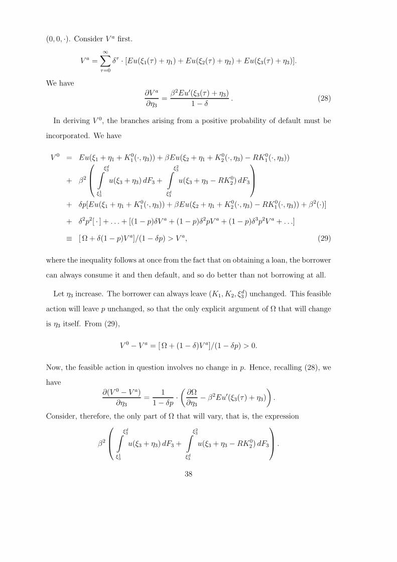
(0, 0, ·). Consider V a first.

V a =∞∑

τ=0

δτ · [Eu(ξ1(τ) + η1) + Eu(ξ2(τ) + η2) + Eu(ξ3(τ) + η3)].

We have∂V a

∂η3=

β2Eu′(ξ3(τ) + η3)

1− δ. (28)

In deriving V 0, the branches arising from a positive probability of default must be

incorporated. We have

V 0 = Eu(ξ1 + η1 +K01(·, η3)) + βEu(ξ2 + η1 +K0

2 (·, η3)−RK01 (·, η3))

+ β2

⎛

⎜⎝

ξd3∫

ξ13

u(ξ3 + η3) dF3 +

ξ23∫

ξd3

u(ξ3 + η3 − RK02) dF3

⎞

⎟⎠

+ δp[Eu(ξ1 + η1 +K01(·, η3)) + βEu(ξ2 + η1 +K0

2 (·, η3)−RK01 (·, η3)) + β2(·)]

+ δ2p2[ · ] + . . .+ [(1− p)δV a + (1− p)δ2pV a + (1− p)δ3p2V a + . . .]

≡ [Ω+ δ(1− p)V a]/(1− δp) > V a, (29)

where the inequality follows at once from the fact that on obtaining a loan, the borrower

can always consume it and then default, and so do better than not borrowing at all.

Let η3 increase. The borrower can always leave (K1, K2, ξd3) unchanged. This feasible

action will leave p unchanged, so that the only explicit argument of Ω that will change

is η3 itself. From (29),

V 0 − V a = [Ω+ (1− δ)V a]/(1− δp) > 0.

Now, the feasible action in question involves no change in p. Hence, recalling (28), we

have∂(V 0 − V a)

∂η3=

1

1− δp·(∂Ω

∂η3− β2Eu′(ξ3(τ) + η3)

).

Consider, therefore, the only part of Ω that will vary, that is, the expression

β2

⎛

⎜⎝

ξd3∫

ξ13

u(ξ3 + η3) dF3 +

ξ23∫

ξd3

u(ξ3 + η3 − RK02) dF3

⎞

⎟⎠ .

38

Since, by hypothesis, K1 and K2 are left unchanged, we have

∂Ω

∂η3= β2

⎛

⎜⎝

ξd3∫

ξ13

u′(ξ3 + η3) dF3 +

ξ23∫

ξd3

u′(ξ3 + η3 − RK02) dF3

⎞

⎟⎠ > β2Eu′(ξ3 + η3)

whenever K2 > 0 in virtue of the strict concavity of u. It follows at once that V 0 − V a

is increasing in η3.

To complete this preliminary step, observe that total differentiation of (4) yields

∂ξd3/∂K2 = −Ru′(ξd3 + η3 − RK2) + δ · ∂(V 0 − V a)/∂η3u′(ξd3 + η3 − RK2)− u′(ξd3 + η3)

,

whose sign is the same as the expression in Section 2.1 when the changes in (η1, η2, η3)

are confined to the current period. It is then straightforward to show that all of the

comparative static results in Section 2 also hold in the setting in which the changes in

(η1, η2, η3) are permanent.

39

References

[1] Afridi, F., Iversen V., and Sharan M. R. (2013), ‘Women political leaders, corrup-

tion and learning: Evidence from a large public program in India’, IZA Discussion

Paper 7212 and International Growth Centre (IGC) Working Paper.

[2] Azam, M. (2012), ‘The Impact of Indian job guarantee scheme on labor market

outcomes: Evidence from a natural experiment’, IZA Discussion Paper 6548.

[3] Bardhan, P. (1983), ‘Labor-tying in a poor agrarian economy: A theoretical and

empirical analysis’, The Quarterly Journal of Economics, 98(3): 501-514.

[4] Bardhan, P., Mookherjee, D., and Torrado M. P. (2010), ‘Impact of political reser-

vations in West Bengal local governments on anti-poverty targeting’, Journal of

Globalization and Development, 1(1): 1-36.

[5] Ban, R., and Rao V. (2008), ‘Tokenism or agency? The impact of women’s reser-

vations on panchayats in south India’, Economic Development and Cultural Change,

56: 501-530.

[6] Basu, A.K. (2013), ‘Impact of rural employment guarantee schemes on seasonal

labor markets: Optimum compensation and workers’ welfare’, Journal of Economic

Inequality, 11(1): 1-34.

[7] Bell, C., Srinivasan, T.N., and Udry, C. (1997), ‘Rationing, spillover, and interlink-

ing in credit markets: The case of rural Punjab’, Oxford Economic Papers, 49(4):

557-585.

[8] Besley, T., Montalvo J. G., and Reynal-Querol M. (2011), ‘Do Educated Leaders

Matter?’, The Economic Journal, 121(554): 205-227.

[9] Chattopadhyay, R., and Duflo E. (2004), ’Women as policy makers: Evidence from

a randomized policy experiment in India’, Econometrica, 72(5): 1409-43.

40

[10] Dey, S., and Imai K. (2014), ‘Workfare as collateral: The case of National Rural

Employment Guarantee Scheme (NREGS) of India’, Economic Discussion Paper No.

1412, Economics Department, University of Manchester.

[11] Gehrke, E. (2014), ‘An employment guarantee at risk insurance? Assessing the

effects of the NREGS on agricultural production decisions’, BGPE Discussion Paper,

No. 152.

[12] Hatlebakk, M. (2009), ‘Capacity-constrained collusive price discrimination in the

informal rural credit markets of Nepal’, Review of Development Economics, 13(1):

70-86.

[13] Imbert, C., and Papp J. (2015), Labor market effects of social programs: Evi-

dence from India’s employment guarantee’, American Economic Journal: Applied

Economics, 7(2): 233-63.

[14] Klonner, S., and Oldiges C. (2014), ‘Safety net for India’s poor or waste of public

funds? Poverty and welfare in the wake of the world’s largest job guarantee program’,

AWI Discussion Paper Series No. 564, University of Heidelberg.

[15] McManus, J. (2014), ‘Educational Qualifications of Village Leaders in North India:

Implications for Public Service Delivery, mimeo, Harvard University.

[16] Raghunathan, N., and Fields, G. (2014), ‘For better or for worse? The effects of an

employment guarantee in a seasonal agricultural market’, mimeo, Cornell University.

[17] Raghunathan K., and Hari S. (2014), ‘Providing more than just employment?

Evidence from the NREGA in India’, mimeo, Cornell University.

[18] Rajaraman I., and Gupta, M. (2012), ‘Public expenditure choices and gender

quotas’, Indian Growth and Development Review, 5(2): 108-130.

[19] Saraswat, D. (2011), ‘Effect of employment guarantee on access to credit: Evidence

from rural India’, MPRA Paper No. 34671.

41

[20] van Dillen, S. (2008), ‘Income and its variability in a drought-prone region: Sea-

sonality, location and household characteristics’, European Journal of Development

Research, 20(4): 579-596.

[21] Zimmermann, L. (2014), ‘Why guarantee employment? Evidence from a large

Indian public-works program’, mimeo, University of Georgia.

42

!!!!!

!!!!!

0!5!10!15!20!25!30!35!

March! April! May! June! July! Aug! Sept! Oct! Nov! Dec!

Num

ber'of'Loans'

Months'

Figure'1:'Monthwise'Total'Number'of'Loans'Taken'

Agricultural!Inputs! Consumption! Funeral! Medical!Expenditures! Other!Purposes!

0!

0.05!

0.1!

0.15!

0.2!

0.25!

Jan! Feb! Mar! April! May! June! July! Aug! Sept! Oct! Nov! Dec!Proportion'of'Yearly'Paym

ent'

Figure'2:'Monthly'Distribution'of'NREGS'Payments'

2012! 2013!

Table 1: Summary StatisticsVariable Obs Mean Std. Dev.

Household has taken loan: yes=1, 0 otherwise 279 .43 .5Total amount of loan (Rs.) 279 5105.81 9598.95Household has taken a consumption loan: yes=1, 0 otherwise 279 .27 .44Total amount of consumption loan (Rs.) 279 2215.05 5989.68Household has taken a production loan: yes=1, 0 otherwise 279 .22 .41Total amount of production loan (Rs.) 279 2890.76 7494.14Household has participated in NREGS: yes=1, 0 otherwise 279 .29 .45Number of days the household has worked on NREGS in the year 279 14.29 32.85Household belongs to General or Scheduled Caste 279 .37 .48Household belongs to Scheduled Tribe 279 .19 .39Household belongs to Other Backward Castes 279 .44 .5Land owned (in acres) 279 1.99 2.13Household has a Below Poverty Line Card 279 .7 .46Household size 279 4.97 2.01Proportion of adults (20+) who are male 279 .3 .17Average age of household members 279 31.67 12.33Years of education for the most educated person in the household 279 5.88 4.03Total number of episodes of morbidity in the household (Jan-Dec) 279 2.22 1.94Total number of deaths in the household (Jan-Dec) 279 .03 .16Total number of households registered for NREGS work 279 137.52 87.18Village development Index Quartile: 4 (most developed) 279 .26 .44Village development Index Quartile: 3 279 .25 .44Village development Index Quartile: 2 279 .26 .44Village development Index Quartile: 1 (least developed) 279 .23 .42Total village area (acres) 279 291 144.5Proportion of village land irrigated 279 .04 .06Distance to district centre (kms.) 279 71.87 28Distance to block centre (kms.) 279 14.37 7.24Distance to panchayat o¢ce (kms.) 279 3.81 1.91Distance to closest bank (kms.) 279 9.3 3.87Distance to closest cooperative society (kms.) 279 5.15 2.96Village has a self help group, yes=1, 0 otherwise 279 .78 .41Credit Market Competition: competitive=1, 0 otherwise 279 .82 .38Education of the sarpanch (yrs) 279 9.41 3.31Sarpanch seat is reserved for a woman 279 .29 .45

Table

2:Sum

mary

StatisticsbyNREGSparticipation

Variable

NREGS(A)

NonNREGS(B)

Twosided

tTest

Mean

Std.Dev.

Mean

Std.Dev.

A−B

Household

hastaken

loan:yes=

1,0otherw

ise.44

.5.42

.49.025

Total

amount

ofloan

(Rs.)

44357461

538010351

−945

Household

hastaken

aconsum

ptionloan:

yes=1,0otherw

ise.23

.43.28

.45−.05

Total

amount

ofconsum

ptionloan

(Rs.)

9812366

27206890

-1738∗∗

Household

hastaken

aproduction

loan:yes=

1,0otherw

ise.26

.44.2

.4.06

Total

amount

ofproduction

loan(Rs.)

34537261

26617593

792Household

hasparticipated

inNREGS:yes=

1,0otherw

ise1

00

0.

Numberofdays

thehousehold

hasworked

onNREGSinthe

year49.23

44.810

049.23

∗∗∗

Household

belongs

toGeneral

orScheduled

Caste

.3.46

.4.49

−.10

∗

Household

belongs

toScheduled

Tribe

.09.28

.23.42

−.14

∗∗∗

Household

belongs

toOther

Backw

ardCastes

.62.49

.37.48

.25∗∗∗

Land

owned

(inacres)

2.12

2.141.93

2.13.19

Household

hasaBelow

Poverty

Line

Card

.78.42

.67.47

.11∗

Household

size5.32

2.264.83

1.89.49

∗

Proportion

ofadults

(20+)whoare

male

.33.18

.29.17

.04∗

Average

ageofhousehold

members

29.77

10.2132.44

13.04−2.68

∗

Years

ofeducation

forthe

most

educatedperson

inthe

household6.33

3.665.69

4.17.64

Total

numberofepisodes

ofmorbidity

inthe

household(Jan-D

ec)2.41

22.14

1.92.27

Total

numberofdeaths

inthe

household(Jan-D

ec).01

.11.03

.17−.02

Total

numberofhouseholds

registeredfor

NREGSwork

12480

14390

−19∗

Village

development

IndexQuartile:

4(most

developed)

.21.41

.28.45

−.07

Village

development

IndexQuartile:

3.23

.43.26

.44−.03

Village

development

IndexQuartile:

2.35

.48.22

.42.12

∗∗

Village

development

IndexQuartile:

1(least

developed)

.21.41

.24.43

−.03

Total

villagearea

(inacres)

28410.41

30615.65

−22

Proportion

ofvillage

landirrigated

.05.06

.04.06

0.01Distance

todistrict

centre(km

s.)69.35

28.7572.91

27.7−3.56

Distance

toblock

centre(km

s.)16

8.0213.71

6.82.29

∗∗

Distance

topanchayat

o¢ce(km

s.)4.09

1.943.69

1.89.39

Distance

toclosest

bank(km

s.)8.78

3.069.52

4.14−.74

Distance

toclosest

cooperative

society(km

s.)5.35

3.035.08

2.93.27

Village

hasaself

helpgroup,

yes=1,0otherw

ise.88

.33.74

.44.13

∗∗

Credit

Market

Competition:

competitive=

1,0otherw

ise.78

.42.84

.37.06

Education

ofthe

sarpanch(yrs)

9.26

2.779.47

3.51−.21

Sarpanchseat

isreserved

forawoman

.2.4

.32.47

−.12

∗∗

Number

ofObservations

81198

Note:

Thedi§erences

maynot

match

duetorounding

o§.*:10%,**:

5%***:

1%

Table 3: Probability of BorrowingOLS Instrumental Variable

(1) (2) (3) (4) (5) (6)VARIABLES LA LC LP LA LC LP

Household has participated in NREGS: yes=1, 0 otherwise -0.03 -0.04 -0.02 0.18 -0.25* 0.60*(0.08) (0.07) (0.07) (0.31) (0.14) (0.32)

Household belongs to Scheduled Tribe -0.01 0.02 -0.02 0.01 -0.00 0.05(0.09) (0.09) (0.07) (0.09) (0.08) (0.09)

Household belongs to Other Backward Castes -0.02 -0.09 0.05 -0.04 -0.07 -0.02(0.08) (0.06) (0.08) (0.08) (0.07) (0.08)

Proportion of adults (20+) who are male -0.02 -0.03 -0.00 -0.08 0.04 -0.20(0.20) (0.18) (0.15) (0.21) (0.17) (0.21)

Land owned (in acres) 0.00 -0.01 0.01 0.01 -0.01 0.03(0.02) (0.01) (0.02) (0.02) (0.01) (0.02)

Household has a Below Poverty Line Card -0.01 -0.06 0.03 -0.02 -0.04 -0.02(0.07) (0.07) (0.06) (0.07) (0.07) (0.07)

Household size 0.02 0.00 0.02 0.02 0.01 0.00(0.01) (0.01) (0.01) (0.02) (0.01) (0.01)

Average age of household members -0.00 -0.00 -0.00 -0.00 -0.00* -0.00(0.00) (0.00) (0.00) (0.00) (0.00) (0.00)

Years of education for the most educated person in the household -0.01* -0.01* -0.01 -0.01** -0.01* -0.01(0.01) (0.01) (0.01) (0.01) (0.01) (0.01)

Total number of episodes of morbidity in the household (Jan-Dec) 0.05*** 0.05*** 0.03* 0.05*** 0.05*** 0.02(0.02) (0.01) (0.01) (0.02) (0.01) (0.02)

Total number of deaths in the household (Jan-Dec) 0.44*** 0.48** 0.17 0.47*** 0.45** 0.27(0.15) (0.21) (0.16) (0.16) (0.19) (0.19)

Total number of households registered for NREGS work -0.00 0.00 -0.00** -0.00 0.00 -0.00***(0.00) (0.00) (0.00) (0.00) (0.00) (0.00)

Village development Index Quartile: 4 (most developed) 0.09 0.07 -0.10 0.03 0.13 -0.26(0.28) (0.15) (0.25) (0.24) (0.18) (0.21)

Village development Index Quartile: 3 0.07 0.02 0.05 0.02 0.06 -0.08(0.18) (0.10) (0.19) (0.18) (0.11) (0.20)

Village development Index Quartile: 2 0.21 0.20** 0.10 0.15 0.25*** -0.05(0.14) (0.07) (0.14) (0.17) (0.08) (0.17)

Total village area (2013) -0.18 -0.21 -0.16 -0.18 -0.15 -0.30(0.35) (0.21) (0.31) (0.35) (0.21) (0.48)

Proportion of village land irrigated -0.75 -0.68 -0.35 -0.70 -0.63 -0.45(0.86) (0.49) (0.90) (0.76) (0.54) (0.89)

Education of the sarpanch (yrs) -0.00 0.01 -0.01 -0.00 0.01 -0.02*(0.02) (0.01) (0.01) (0.02) (0.01) (0.01)

Distance to district centre (kms.) 0.00 0.00 0.00 -0.00 0.00 -0.01(0.00) (0.00) (0.00) (0.00) (0.00) (0.00)

Distance to panchayat o¢ce (kms.) 0.02 0.02 -0.02 0.01 0.03* -0.04(0.03) (0.01) (0.02) (0.03) (0.01) (0.03)

Distance to block centre (kms.) -0.01 -0.01* -0.00 -0.01 -0.01** 0.00(0.01) (0.00) (0.01) (0.01) (0.00) (0.01)

Distance to closest bank (kms.) -0.00 0.00 -0.01 -0.00 0.00 -0.00(0.01) (0.01) (0.01) (0.01) (0.01) (0.01)

Distance to closest cooperative society (kms.) 0.02 0.00 0.01 0.01 0.01 0.00(0.02) (0.01) (0.02) (0.02) (0.01) (0.02)

Village has a self help group, yes=1, 0 otherwise 0.05 0.06 0.05 0.01 0.12** -0.10(0.08) (0.06) (0.07) (0.12) (0.05) (0.12)

Credit Market Competition: competitive=1, 0 otherwise -0.05 -0.05 -0.01 -0.02 -0.09 0.09(0.13) (0.09) (0.13) (0.14) (0.07) (0.16)

Constant 0.20 0.25 0.28 0.56 -0.12 1.37(0.95) (0.58) (0.85) (0.93) (0.68) (0.91)

Block Fixed E§ects YES YES YES YES YES YES

Observations 279 279 279 279 279 279R-squared 0.174 0.168 0.180

First Stage: Sarpanch seat is reserved for a woman -.39∗∗∗

F stat 14.65∗∗∗

Kleibergen-Paap rk Wald F statistic 14.65 (15% Value: 8.96)Robust standard errors in parentheses; *** p<0.01, ** p<0.05, * p<0.1

Table 4: Amount Borrowed (Rs.)IV Tobit

(1) (2)VARIABLE KC KP

Number of days the household has worked on NREGS in the year -273* 963**(141.6) (387.06)

All other Covariates YES YES

Number of observations 279 279Number of censored observations 204 218

Wald Test of Exogeneity 2.57 5.99**

First StageSarpanch seat is reserved for a woman -23.6***

Marginal E§ect conditional on Kj > 0 -73* 277**Robust clustered standard errors in parentheses *** p<0.01, ** p<0.05, * p<0.1

Table 5: Seasonal E§ectsIV -LPM IV Tobit(1) (2) (3) (4)

VARIABLE L KL1 L2 K1 K2

Household has participated in NREGS: yes=1, 0 otherwise -.19** .61(.08) (.42)

Number of days the household has worked on NREGS in the year -1421** 442.2*(574) (250)

All other Covariates# YES YES YES YES

Number of observations 279 279 279 279Number of censored observations 253 184

Marginal E§ect conditional on Ki > 0 -373** 138*#In columns (1) and (3) that correspond to season 1, we use the total number of sickness episodes

in the rabi season to measure morbidity. Robust clustered standard errors in parentheses *** p<0.01, ** p<0.05, * p<0.1

Table 6: Robustness(1) (2) (3) (4) (5) (6) (7) (8)

LC LP

VARIABLES

Household has participated in NREGS: yes=1, 0 otherwise -0.25* -0.26** -0.26* -0.26*** 0.61* 0.61* 0.69* 0.66**(0.14) (0.12) (0.15) (0.08) (0.34) (0.34) (0.36) (0.28)

Baseline YES YESOutstanding Loan YES YESDistance to nearest All Weather Road YES YESExpenditure on Other Schemes YES YES

Number of observations 279 279 279 251 279 279 279 251Robust clustered standard errors in parentheses *** p<0.01, ** p<0.05, * p<0.1

TableA.1:

Village

Level

NREGS(2013)

(1)(2)

(3)(4)

VARIABLES

#ofNREGSHH.s

#ofNREGSHH.s

#ofNREGSHH.s

#ofNREGSHH.s

Sarpanchseat

isreserved

forawoman

-32.746-49.165**

-51.166**(20.607)

(19.129)(21.339)

Sarpanchseat

isreserved

foraScheduled

Caste

-15.489-17.643

(25.716)(23.513)

Sarpanchseat

isreserved

foraScheduled

Tribe

-20.925-0.496

(24.015)(23.538)

Village

Developm

entIndex

-5.443-3.052

-5.072(4.584)

(5.286)(4.903)

Total

numberofhouseholds

registeredfor

NREGSwork

0.308***0.226*

0.311***(0.102)

(0.112)(0.108)

Rainfall

Deviation

(2013)from

longrun

average0.598

0.5280.452

(0.790)(0.917)

(0.838)Constant

56.190***29.295

32.48630.771

(11.287)(20.806)

(25.431)(23.247)

Observations

3030

3030

R-squared

0.0830.347

0.2040.363

Standarderrors

inparentheses

***p<0.01,

**p<0.05,

*p<0.1

TableA.2:V

illageLevel

NREGS(2013)

(1)(2)

(3)(4)

VARIABLES

#ofNREGSPersondays

#ofNREGSPersondays

#ofNREGSPersondays

#ofNREGSPersondays

Sarpanchseat

isreserved

forawoman

-985.540-1,532.623*

-1,843.814*(877.503)

(866.192)(963.940)

Sarpanchseat

isreserved

foraScheduled

Caste

-58.641-136.264

(1,118.619)(1,062.148)

Sarpanchseat

isreserved

foraScheduled

Tribe

84.604820.787

(1,044.647)(1,063.286)

Village

Developm

entIndex

-332.353-296.617

-369.403(207.551)

(229.943)(221.469)

Total

numberofhouseholds

registeredfor

NREGSwork

10.090**7.951

10.994**(4.625)

(4.860)(4.878)

Rainfall

Deviation

(2013)from

longrun

average-6.732

-9.445-12.181

(35.752)(39.891)

(37.876)Constant

2,314.429***996.583

773.578711.788

(480.628)(942.107)

(1,106.262)(1,050.145)

Observations

3030

3030

R-squared

0.0430.229

0.1330.252

Standarderrors

inparentheses

***p<0.01,

**p<0.05,

*p<0.1

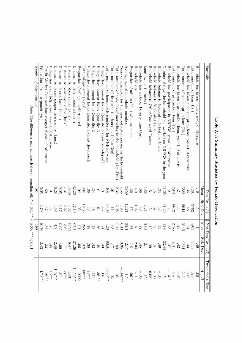
TableA.3:

Summary

Statistics

byFemale

Reservation

Variable

FemRes.

(A)

NotFem

Res.

(B)

Twosided

tTest

Mean

Std.Dev.

Mean

Std.Dev.

A−B

Household

hastaken

loan:yes=

1,0otherw

ise.49

.5.4

.49.09

Total

amount

ofloan

(Rs.)

55909792

49119538

678Household

hastaken

aconsum

ptionloan:

yes=1,0otherw

ise.35

.48.24

.43.11

∗

Total

amount

ofconsum

ptionloan

(Rs.)

23885044

21466341

242Household

hastaken

aproduction

loan:yes=

1,0otherw

ise.2

.4.23

.42−.03

Total

amount

ofproduction

loan(Rs.)

32038612

27657015

437Household

hasparticipated

inNREGS:yes=

1,0otherw

ise.2

.4.33

.47−.13

∗∗

Numberofdays

thehousehold

hasworked

onNREGSinthe

year11.05

31.2915.6

33.44−4.54

Household

belongs

toGeneral

orScheduled

Caste

.34.48

.39.49

−.05

Household

belongs

toScheduled

Tribe

.16.37

.2.4

−.03

Household

belongs

toOther

Backw

ardCastes

.5.5

.42.49

0.08Land

owned

(inacres)

1.88

2.212.03

2.1−.15

Household

hasaBelow

Poverty

Line

Card

.66.48

.72.45

−.06

Household

size4.9

1.975

2.04−.1

Proportion

ofadults

(20+)whoare

male

.26.15

.31.18

−.06

∗∗

Average

ageofhousehold

members

30.59

12.7132.1

12.17−1.5

Years

ofeducation

forthe

most

educatedperson

inthe

household4.55

3.966.41

3.95−1.86

∗∗∗

Total

numberofepisodes

ofmorbidity

inthe

household(Jan-D

ec)2.34

2.082.17

1.89.16

Total

numberofdeaths

inthe

household(Jan-D

ec).01

.11.03

.17−.02

Total

numberofhouseholds

registeredfor

NREGSwork

16696.09

12680.81

39.86

∗∗∗

Village

development

IndexQuartile:

4(most

developed)

.3.46

.24.43

.06Village

development

IndexQuartile:

30

0.36

.48−.36

∗∗∗

Village

development

IndexQuartile:

2.34

.48.23

.42.11

∗

Village

development

IndexQuartile:

1(least

developed)

.36.48

.18.38

.19∗∗∗

Total

villagearea

(acres)348

12.66268

10.8

80∗∗∗

Proportion

ofvillage

landirrigated

.04.05

.04.06

−.0002

Distance

todistrict

centre(km

s.)82.26

27.1967.7

27.2914.56

∗∗∗

Distance

toblock

centre(km

s.)15.46

8.8213.93

6.471.53

Distance

topanchayat

o¢ce(km

s.)4.31

2.273.6

1.7.71

∗∗∗

Distance

toclosest

bank(km

s.)9.95

3.179.05

4.09.9∗

Distance

toclosest

cooperative

society(km

s.)6.28

3.684.7

2.481.57

∗∗∗

Village

hasaself

helpgroup,

yes=1,0otherw

ise.9

.3.73

.44.16

∗∗∗

Credit

Market

Competition:

competitive=

1,0otherw

ise.69

.47.87

.33−.19

∗∗∗

Education

ofthe

sarpanch(yrs)

6.05

2.7910.76

2.43−4.71

∗∗∗

Number

ofObservations

80199

Note:

Thedi§erences

maynot

match

duetorounding

o§.∗<0.1,

∗∗<0.05,

∗∗∗<0.01