Incarceration of African American Men and

the Impacts on Women and Children

Job Market Paper

Latest draft available online at http://stanford.edu/~sitian/sitianJMP_paper

Sitian Liu∗

Stanford University

December 11, 2018

Abstract

Since the early 1970s, the United States has experienced a dramatic surge in impris-onment, especially among African American men. This paper investigates the causaleffects of black male incarceration on black women’s marriage and labor market out-comes, as well as its effects on black children’s family structure, long-run educationaloutcomes, and income. To establish causality, I exploit plausibly exogenous changesin sentencing policies across states and over years, and construct a simulated instru-mental variable for the incarceration rate, using offender-level data on the universe ofprisoners admitted to and released from prisons between 1986 and 2009. The instru-ment characterizes how sentencing policies affect incarceration at both the extensivemargin (i.e., whether to incarcerate an arrestee) and the intensive margin (i.e., howlong to imprison an inmate). First, I find that high incarceration rates of black mennegatively affect black women’s marriage outcomes, although they increase the likeli-hood of employment for those with higher education levels. Second, higher black maleincarceration rates hurt black children by increasing the likelihood of out-of-wedlockbirth and living in a mother-only family, and decreasing the likelihood of having somecollege education in the long run. Moreover, for individuals who lived in areas withharsher sentencing policies during childhood, the black-white income gap is wider formen conditional on parental income. Third, black men at either the extensive or inten-sive margin of incarceration have different impacts on women and children. The resultssuggest the consequences of the tough-on-crime policies for inequality and racial gaps,which could be taken into account when reforming sentencing policies.

∗Department of Economics. 579 Serra Mall, Stanford, CA 94305. Email: sitian@stanford.edu. I amgrateful to my advisors, Caroline M. Hoxby, Rebecca Diamond, Petra Persson, and Luigi Pistaferri, fortheir guidance and support. I also thank Jaime Arellano-Bover, Yiwei Chen, John Donohue, Mark Duggan,Eleonora Freddi, Shota Ichihashi, David Alan Sklansky, Isaac Sorkin, Yichen Su, and participants at theStanford Labor Seminar, Applied Lunch, Labor and Public Workshop, and San Fransisco State UniversityEconomics Seminar. I acknowledge financial support from the John M. Olin Program in Law and EconomicsResearch Fellowship and the B.F. Haley and E.S. Shaw Fellowship for Economics.

1 Introduction

Over the past four decades, the United States has witnessed dramatic growth in incarceration,

with a 1.1 million increase in the number of adults in state or federal prisons between 1974

and 2001, up from 216,000; the phenomenon is broadly described as “mass incarceration”

(Bonczar, 2003). The African American population, and in particular African American

men, has been disproportionately affected by mass incarceration: 11% of black men between

20 and 39 years old were in state or federal prisons and local jails, compared with 1.7% of

white men, 1% of black women, and 0.2% of white women in that age group as of 2001.1

This paper investigates the causal effects of the incarceration of African American men

on women’s marriage and labor market outcomes, as well as children’s family structure, long-

run educational outcomes, and income. I construct a simulated instrumental variable (IV)

for the incarceration rate of black men, which exploits variation in sentencing policies across

states and over years. Using household data on women and children between 1986 and 2009,

linked with the incarceration rate of black men by year and metropolitan statistical area

(MSA), I find that higher incarceration rates of black men negatively affect black women’s

marriage outcomes, although they increase the probability of employment for relatively more

educated black women. They also have negative consequences for children’s family struc-

ture and long-run educational outcomes. Moreover, for individuals who lived in areas with

harsher sentencing policies during childhood, the black-white income gap is wider for men

conditional on parental income. Lastly, black men at either the extensive or intensive margin

of incarceration have different impacts on women’s and children’s outcomes.

A challenge in estimating the causal impact of incarceration is the potential endogeneity

problem: Increases in the incarceration rate can be correlated with unobservable changes

in social norms, economic factors, local conditions, or individual characteristics that may

affect women’s and children’s economic outcomes independently. To overcome endogeneity,

I exploit plausibly exogenous changes in state and federal sentencing policies and build a

1Estimation is based on the number of inmates in state or federal prisons and local jails by gender, race,Hispanic origin, and age on June 30, 2001, from Prison and Jail Inmates at Midyear 2001 from the Bureau ofJustice Statistics (Beck et al., 2002), and the July 1 resident population, by gender, race, Hispanic origin, andage, from Bridged-Race Population Estimates on the CDC Wonder website (https://wonder.cdc.gov/bridged-race-population.html).

1

simulated IV for the incarceration rate. The IV characterizes how sentencing policies affect

incarceration at both the extensive margin (i.e., whether to incarcerate an arrestee) and

the intensive margin (i.e., how long to imprison an inmate). The IV strategy essentially

uses a difference-in-differences (DD) strategy to estimate the impact of sentencing policy

changes. To illustrate how the simulated IV works, consider different sentences for theft

due to different sentencing policies across states and over years. Suppose Person A stole a

$400 pair of basketball shoes in Georgia and Person B stole similar items in Florida, but

they are otherwise identical. Person A would be charged with a misdemeanor and punished

with a fine. However, Person B would be charged with a felony and might have to serve

time in prison. Moreover, Florida implemented truth in sentencing in 1995, which requires

that all offenders serve a substantial portion of the sentence before being eligible for release.

Therefore, Person B might have to serve longer time in prison if he was sentenced after 1995.

With the simulated IV, I estimate causal effects of “missing” black men at the margins

of incarceration, where the punitiveness of sentencing policies influences whether they would

be incarcerated conditional on arrest, and for how long. Moreover, men with some form

of contact with the criminal justice system and those with longer duration of incarceration

could have different impacts on women and children (e.g., Andersen, 2016; Massoglia et al.,

2011; Pager, 2003). By constructing simulated IVs that exploit changes in sentencing policies

at different margins separately, I disentangle the impacts of (1) “missing” black men at the

extensive margin of incarceration (i.e., men who serve short terms of imprisonment and

would not have been incarcerated at all under less harsh sentencing laws), and (2) “missing”

black men at the intensive margin of incarceration (i.e., men who serve longer terms of

imprisonment and would have been released more quickly under less harsh sentencing laws).

To construct the simulated IV, I employ offender-level data on the universe of prisoners

who were admitted to or released from state or federal prisons between 1983 and 2009 from

the National Corrections Reporting Program (NCRP) and arrest data from the Uniform

Crime Reporting (UCR) Program. The data allow me to estimate the variables used to

construct the IV: (1) probability of incarceration conditional on arrest and (2) average time

served in prison by year of prison admission, state or MSA where sentence was imposed,

offense, race, and gender. Furthermore, I estimate the incarceration rate of adult black men

2

by year and MSA of sentence using data from the NCRP and U.S. Census Population Data.

To examine how black male incarceration affects black women and children, I merge the in-

carceration rates with individual-level information on marriage, employment, education, and

family structure by year and MSA between 1986 and 2009. It is noteworthy that the incar-

ceration rate is only one measure of the percentage of individuals who are “disabled” in the

marriage market due to harsh sentencing policies. Nevertheless, the results also reflect the

impacts of other outcomes associated with incarceration that are driven by harsh sentenc-

ing policies, such as probation, parole, or previous incarceration. In particular, incarceration

leaves in its wake a large population of former prisoners residing among the noninstitutional-

ized population who face health problems, difficulty finding employment, and social stigma.

They are “disabled” by incarceration, becoming less viable as potential marriage partners in

life.

My results suggest that the surging incarceration rates of black men negatively affect

black women’s marriage outcomes. For example, I find that a 1 pp increase in the black

male incarceration rate lowers the likelihood of marriage by 3 pp and lowers the likelihood

of “marrying up” by 2 pp for black women between the ages of 18 and 34.2 Also, more

educated black women are more likely to be employed in the face of higher black male incar-

ceration rates. Moreover, my results indicate that mass black male incarceration could hurt

children by negatively affecting family structure and their long-run educational outcomes.

For example, I find that for black children, a 1 pp increase in the incarceration rate of black

men increases the likelihood of being born out of wedlock and living in a mother-only family

by 4.3 pp and 3.5 pp, respectively; in the long run, it lowers the likelihood of obtaining at

least some college education by 3.8 pp. Finally, my results suggest that harsh sentencing

policies could partially explain the large intergenerational gap in income between black and

white men. I find that a 1 standard deviation (SD) increase in the punitiveness of sentencing

policies in areas where individuals lived during childhood increases the gap in income ranks

between black and white men by 0.7 percentile conditional on parental income. It is notewor-

thy that the two-stage least square (2SLS) results are considerably larger in magnitude than

2In this paper, the incarceration rate of black men is defined as the fraction of black men between theages of 20 and 54 who are in prison. “Marrying up” is defined as having a husband whose years of educationare at least equal to the woman’s.

3

the ordinary least squares (OLS) results. This could result from omitted variable bias and

attenuation bias due to measurement error. Another reason could be heterogenous treat-

ment effects. In particular, I find that compliers—marginal prisoners whose imprisonment is

influenced by sentencing policy changes—are more marriageable, and therefore could have

larger impacts on women’s and children’s outcomes.

My results also suggest that black men at different margins of incarceration have different

impacts on women and children. I find that a 1 pp increase in the incarceration rate of black

men at the extensive margin lowers the likelihood of marriage by 4 pp for black women

with some college education, and the impact is small and statistically insignificant for less

educated black women; a 1 pp increase in the incarceration rate of black men at the intensive

margin lowers the likelihood of marriage by 4 pp for black women with no college education,

and the impact is small and statistically insignificant for more educated black women. It

is reasonable that the extensive (intensive) margin incarceration of black men has a starker

effect on the marriage of relatively more (less) educated women. This is because black men at

the extensive margin of incarceration are likely to serve relatively short terms of imprisonment

and would not have been incarcerated at all under less harsh sentencing policies. They are

more likely to have committed less serious crimes, and therefore more likely to be considered

potential marriage partners by more educated black women, and vice versa.3 While both

cases have substantial effects on children, the impact of black men at the intensive margin of

incarceration is notably large: A 1 pp increase in the intensive margin incarceration rate of

black men increases the likelihood of out-of-wedlock birth and living in a mother-only family

before the age of 15 by 7.3 pp and 6.9 pp, respectively. The results suggest that a father’s

longer separation from his family could be especially harmful for children.

In order to interpret the results in a more economically grounded way, I develop a simple

intertemporal model. In it, women make consumption and marriage decisions given their

marriage market conditions, which differ by the male incarceration rate. When making

marriage decisions, a woman faces the trade-off between financial support from the husband

3Black men at the intensive margin of incarceration are likely to serve longer terms of imprisonment andwould have been released more quickly under less harsh sentencing policies. They are more likely to havecommitted more serious crimes, and therefore more likely to be considered potential marriage partners byrelatively less educated black women.

4

and the potential risk that her husband could be incarcerated in the future. Simulation of

the model shows that higher male incarceration rates lower the percentage of women who

marry, and women with higher asset levels are the first to opt out of marriage.

The paper’s contributions are threefold. The first contribution is identification. I exploit

plausibly exogenous changes in sentencing policies across states and over years, and encap-

sulate policy changes efficiently in powerful instruments. Employing the simulated IV not

only increases the power of the first stage by employing a continuous measure of the effects

of complicated sentencing policies, but also improves its clarity by specifying how sentencing

policies fit into the prison population based on a simulation model of the prison population.

The second contribution is measuring the incarceration rate at the MSA level. Public-use

data usually provide incarceration rates at the national or state level, so papers that study

the impact of incarceration mostly conduct analysis at the state level. However, there is

in fact substantial variation in incarceration rates within states. Moreover, MSAs are more

suitable as geographic units for the analysis of marriage and labor markets.4

A concern about using changes in sentencing policies to identify causal impacts of incar-

ceration is the existence of potential confounding factors that may be related to both the

outcome and the sentencing policies, such as crime rates or racial composition. Nevertheless,

I find substantial variation in incarceration rates across MSAs within states, which suggests

that state-level policy changes are not likely to be driven by some common shock faced by

all MSAs.5 More specifically, I do not find a statistically significant correlation between the

simulated IV and the crime rate or the percentage of the black population. Moreover, with

the MSA-level measurement, I am able to construct instruments using leave-one-out means,

which could eliminate the impact of idiosyncratic shocks.6

Finally, my third contribution is that I investigate the long-run impacts of black male

incarceration on children and the impact of sentencing policies on intergenerational gaps in

income. Moreover, by constructing simulated IVs that characterize how sentencing policy

changes affect incarceration at different margins, I am able to estimate different impacts of

4MSAs are regions with a relatively high population density and close economic ties throughout the area.In particular, I combine non-metropolitan areas within each state as a unique MSA of the state.

5I discuss the concern and corresponding robustness checks in Section 5.4 and Section 6.8 in more detail.6Specifically, I construct the simulated IV for MSA m in state s using the sentencing outcomes of offenders

sentenced from state s, leaving out those sentenced from MSA m.

5

“missing” black men at different margins of incarceration.

My results have implications for sentencing policies and other correctional programs. Al-

though many studies have evaluated direct expenditures on corrections and the consequences

of incarceration for former inmates, the broader consequences of incarceration for black fam-

ilies could also have welfare implications. First, my results suggest negative impacts of black

male incarceration on black children’s living circumstances and long-run outcomes and black

women’s marriage outcomes. In particular, lower marriage rates of black women could lower

both their and their children’s welfare because of lower household income. Second, impacts

of black men at the extensive margin of incarceration suggest that there could be indirect

benefits of alternative sentencing to incarceration. Third, my results indicate that black men

at the intensive margin of incarceration have larger effects on less educated black women and

children, which could possibly exacerbate inequality. My results also indicate that the puni-

tiveness of sentencing policies could partially explain the black-white intergenerational gaps

in income. Therefore, the potential consequences of the tough-on-crime policies on inequality

and racial gaps could be taken into account for sentencing policy-making.

The rest of the paper is organized as follows. Section 2 provides a literature review

and Section 3 describes the data and measurement. Section 4 provides some background

information on sentencing policy changes. The empirical strategy is outlined in Section 5

and results presented in Section 6. Section 7 elucidates a theoretical framework to help

interpret the results, and Section 8 concludes.

2 Literature Review

This paper is related to three strands of literature. The first is the literature on sex ratios and

marriage markets.7 The seminal work of Becker (1973, 1974) suggests that a reduction in the

number of men should shift gains from marriage away from women toward men. Following

this, some studies use cross-sectional variation in sex ratios to estimate the relationship

between the sex ratio and the marriage market or female labor supply (Chiappori et al.,

7For a more detailed review of literature on sex ratios and marriage markets, see Abramitzky, Delavande,and Vasconcelos (2011).

6

2002; Cox, 1940; Easterlin, 1961; Guttentag and Secord, 1983). A big challenge in these

studies is that it is hard to find exogenous variation in sex ratios, and therefore there can

be reverse causality. Abramitzky, Delavande, and Vasconcelos (2011) overcome the problem

by exploiting exogenous geographic variation in sex ratios due to war mortality.8 Angrist

(2002) and Lafortune (2013) exploit differences in changes in sex ratios across ethnic groups

over time due to massive immigration. I complement this literature by exploiting exogenous

changes in sentencing policies that contribute to the growth of the prison population. Since

imprisonment is prevalent among the African American population and there is a large

gender gap in incarceration, mass incarceration shrinks the pool of marriageable black men

by removing them from marriage markets to prisons, and reducing their “marriageability”

with criminal records and high risks of incarceration.

This paper is also related to the literature on the impacts of incarceration. A large body

of literature focuses on the direct impact of incarceration on criminal activity and the con-

sequences for former inmates, such as later criminal behaviors, human capital formation,

employment, wages, health, and family relationships (Aizer and Doyle Jr, 2015; Kuziemko

and Levitt, 2004; Levitt, 1996; Mueller-Smith, 2015; Western and Lopoo, 2004; Western and

McClanahan, 2000; Western, 2002; Wildeman and Muller, 2012).9 Nevertheless, collateral

impacts of aggregate male incarceration have been less studied. To the best of my knowledge,

Charles and Luoh (2010) and Mechoulan (2011) are the first to investigate the relationship

between male incarceration and female outcomes.10 These studies use variation in male incar-

ceration rates across states and over years, and attempt to address the potential endogeneity

problem by controlling for observable characteristics or state-specific time trends. The fixed

effect approach assumes that changes in incarceration rates are not correlated with changes

in unobservable confounds that may affect female outcomes within marriage markets (states)

over time.11 Therefore, their results may not represent a causal relationship because of un-

8Brainerd (2017) uses similar variation in the context of Russia.9Some studies also investigate the impact of incarceration on African American communities by exploiting

the geographic concentration of incarceration (Clear, 2008). Influential work by Johnson and Raphael (2009)studies the impact of male incarceration on AIDS infection.

10Caucutt et al. (2016) develop an equilibrium search model of marriage, divorce, and labor supply. Theyshow that differences in incarceration and employment between black and white men can explain part of theblack-white marriage gap.

11A more detailed review of these studies is presented in Appendix A1.

7

observable confounds, such as criminal or police behaviors. I propose a simulated IV that

exploits changes in sentencing policies to address the potential endogeneity of incarceration.

Moreover, I conduct analysis at the MSA level, which allows me to construct the IV using

leave-out-the-own-MSA method. This eliminates the impact of local idiosyncratic shocks,

such as changes in local criminal activity or local judge behaviors, and therefore addresses

the endogeneity issue associated with state-level studies, including Charles and Luoh (2010)

and Mechoulan (2011). Finally, I add to these studies by estimating long-run impacts on

children and intergenerational income gaps.

Lastly, this paper is related to the literature on how changes in sentencing policies affect

the prison population. One strand of the literature uses panel regressions to determine how

a particular sentencing policy change affects the prison population (Nicholson-Crotty, 2004;

Stemen et al., 2006; Stemen and Rengifo, 2011; Zhang et al., 2009). However, there is no

consensus among these studies. Another strand of the literature uses simulation models to

decompose different factors that contribute to the growth of the prison population (Blumstein

and Beck, 1999; Neal and Rick, 2016; Pfaff, 2011; Raphael and Stoll, 2013).12

The construction of the simulated IV is motivated by the simulation models presented

by Raphael and Stoll (2013) and Neal and Rick (2016), which aim to match the simulated

prison population to the real prison population. Instead, I extract exogenous components

of the simulation models that characterize the punitiveness of sentencing policies: tendency

to incarcerate arrestees and time served in prison. Then I use these exogenous components

to construct an IV based on a simulation model of the prison population. This strategy

is essentially a DD research design. However, it it difficult to implement a DD approach

directly to estimate the impact of sentencing policy changes, because many policies were

implemented simultaneously, different states had different requirements for similar laws, and

different states used different names for laws with similar effects. Mixed results among the

studies that identify the effect of each sentencing policy change also suggest that the effects

12Both Neal and Rick (2016) and Raphael and Stoll (2013) use data from the National Corrections Report-ing Program. Raphael and Stoll (2013) develop a steady-state model of the prison population, and Neal andRick (2016) further introduce distributions of time served given arrest. Raphael and Stoll (2013) concludethat an enhanced tendency to sentence convicted offenders to prison and longer sentences contributes tomore than 90% of the difference between the 1984 and 2004 steady-state prison population. Neal and Rick(2016) “document a broad shift toward more punitive treatment for offenders in every major crime category.”

8

of sentencing policy changes are complicated.

3 Data Description and Measurement

3.1 Arrest Data

The Federal Bureau of Investigation (FBI) has compiled the Uniform Crime Reporting Pro-

gram (UCR), which collects data on crimes and arrests through reporting by participating

law enforcement agencies, since 1930. I use yearly summary data that provide information

on the number of arrests by state, year, offense, gender, and age group, as well as the number

of arrests of adults by state, year, offense, and race.

3.2 Prisoner Data

I use data on prisoners from four sources. First, the National Prisoner Statistics Program

(NPS) provides an enumeration of inmates in state and federal prisons since 1926 by various

characteristics. In 1999, the database was expanded to include inmates held in local facilities.

In particular, I use data on jurisdiction population at year end by year, state, race, and gender

between 1983 and 2009.

The main data on prisoners are from the National Corrections Reporting Program (NCRP),

which has collected offender-level administrative data annually since 1983. It consists of data

for the universe of prisoners who were admitted to prison (Admissions Data) or released from

prison (Releases Data) from 1983 to 2009. In 2004, 22 states also began to collect data on

stocks of prisoners in custody at year end (Yearend Population Data). The NCRP data

provide demographic information, including date of birth, gender, race, Hispanic origin, and

education attainment. The data also provide sentencing information, including date of ad-

mission to prison, date of release from prison (in Releases Data only), conviction offense(s),

length of the longest sentence, location where sentence was served, state of custody, and

county (and MSA)13 where sentence was imposed. A more detailed description of the NCRP

data can be found in Appendix A2.1.

13The NCRP provides the county where sentence was imposed. I match counties to MSAs based on the2000 delineation of the Office of Management and Budget.

9

Third, the Survey of Inmates in State Correctional Facilities (SISCF) (1986, 1991, 1997,

and 2004) selects nationally representative samples of inmates in state prisons, and collects

detailed demographic characteristics of prison inmates. In particular, the SISCF data provide

marital status and employment status 1 month before arrest, in addition to the variables

provided in the NCRP. Unfortunately, the samples are not annual, and only provide the

census region (not state) where an inmate was interviewed.

Fourth, I use data from the American Community Survey (ACS) (2006-2009) for demo-

graphic characteristics of individuals in institutions to complement the SISCF data. Unfortu-

nately, the ACS data do not distinguish among different types of institutions. Nevertheless,

when the sample is restricted to young black men in institutions, their characteristics are

comparable to the characteristics of young black male inmates in the SISCF.14

Table 1 provides summary statistics for newly admitted black male prisoners from the

NCRP (Columns 1-2), black male inmates in state prisons from the SISCF (Columns 3-4),

black men in institutions from the ACS (Columns 5-6), and general black male population

from the household data described in the next subsection (Columns 7-8). Compared with

the general black male population, black male inmates are younger, more likely to be single,

and less likely to have higher levels of education. Interestingly, however, the employment

rates of black male inmates before arrest are comparable to that of the general population.

3.3 Household Data

For the dependent variables and individual characteristics of women and children, I use re-

peated cross-sectional data from the Current Population Survey Annual Social and Economic

Supplement (CPS-ASEC) 1986-2009, the American Community Survey (ACS) 2006-2009,

and the U.S. Census 5% samples for 1990 and 2000 from the Integrated Public Use Micro-

data Series (IPUMS). The data provide demographic information, such as age, gender, race,

14The ACS data do not distinguish among different types of institutions, including correctional institutions,mental institutions, and institutions for the elderly, handicapped, or poor. Charles and Luoh (2010) treatyoung men in the 1990 and 2000 censuses characterized as institutionalized as being incarcerated. Theyargue that young men are most likely to be in mental institutions if not incarcerated, but according to Grob(2000), the number of people in mental institutions has plummeted since the 20th century in the UnitedStates. Charles and Luoh (2010) also show that the patterns of incarceration based on the definitions theyuse are consistent with information on incarceration from the Bureau of Justice Statistics.

10

marital status, and family interrelationship, and socioeconomic information, such as edu-

cational attainment, employment status, and income. The geographic information includes

current state, MSA, and county of residence.15 The U.S. Census 5% samples and the ACS

data also provide state of birth.

3.4 Measurement

In this subsection, I describe how I measure the prison population and the incarceration

rate at the MSA level. Public-use data on prisoners provide the number of prisoners at the

national and state level in general.16 However, there is substantial variation in incarceration

rates across areas within states.17 Therefore, it is important to measure the incarceration

rate at the MSA level. And last, I discuss how the incarceration rate should be interpreted.

3.4.1 Prison Population at the MSA Level

The NCRP data did not provide information on stocks of prisoners in custody until 2004.

Therefore, I use the perpetual inventory method to estimate the year-end prison population

by year, MSA of sentence, race, and gender between 1983 and 2009. First, I use the NCRP

data on stocks of prisoners in custody between 2004 and 2009 to estimate the year-end prison

population between 2004 and 2009, by year, MSA of sentence, race, and gender. Second, I

use the NCRP data on admissions and releases between 1983 and 2009 to estimate yearly

changes in prison population—namely the number of admission minus the number of releases

within each year.18 Last, I back out the year-end prison population before 2004. Since only

15The CPS-ASEC provides information on MSA since 1962. The number of MSAs identified increasedover time, from 15 beginning in 1962 to over 200 beginning in 1986. Therefore, I focus on years between1986 and 2009. The CPS-ASEC provides information on county since 1996. I do not use CPS Basic Monthlydata because they started to provide information on MSA in 1994 and on county in 1995.

16The Vera Institute of Justice provides data on the total jail and prison population at the county level(link: https://www.vera.org/projects/incarceration-trends). The institute will publish data on the prisonand jail population count at the county level by race or by gender (but not by both race and gender).

17For instance, in California, 2000, while on average 9.4% of black men ages 20-54 were in prison, lessthan 2% of black men from the MSA of San Luis Obispo County were in prison, and more than 20% ofblack men from the MSA of Shasta County were in prison. For another instance, in Texas, 2000, theaverage incarceration rate was 9.2%. The minimum was less than 0.4% in the MSA of Webb county, andthe maximum was more than 16% in the MSA of Ector County and Midland County.

18I assume that prisoners will return to the MSA where they were sentenced after they are released. Theassumption is reasonable, because their social networks (including family and friends) are likely to remainwhere they used to live. Visher et al. (2008) show that most former prisoners search for a job through family

11

22 states provide data on year-end prison population, I can only estimate MSA-level prison

population for the 22 states. In Appendix A2.2, I discuss in detail the availability and

reliability of the NCRP data across states for the estimation and how I clean the data. In

Appendix A2.3, I show mathematically how I employ the perpetual inventory method to

estimate the prison population at the MSA level.

It is noteworthy that the geographic unit is the MSA where sentence was imposed. There

are three reasons why it is important to use the MSA where sentence was imposed, rather

than the location of custody. First, the MSA of sentence is most likely to be the place where

an offender committed a crime. It is also more likely to be the marriage market where the

person is “missing,” since offenders generally commit crimes near their residence.19 Second,

the number of prisoners held in prisons within a MSA can be different from the number

of prisoners who are sentenced from the MSA, and the latter is a better estimate of the

number of people missing from the marriage market of the MSA.20 Finally, using the MSA

of sentence, transfers of prisoners between different locations do not affect the estimation.21

After the estimation, I check whether the estimated MSA-level year-end prison population

is reliable in two ways. First, I compare the year-end MSA prison population 2004-2008

estimated directly from NCRP Yearend Population Data (Figure 1 x-axes) with the year-

end MSA prison population 2004-2008 backed out using the year-end prison population in

2009 and yearly changes between 2005 and 2009 (Figure 1 y-axes). This checks whether data

on stocks of prisoners in custody are consistent with data on admissions and releases in the

NCRP. Figure 1 shows that the two estimates are almost the same.

Second, I aggregate the estimated MSA prison population to the state level, and compare

or friends, and family or friends are also the most common source of income for formerly incarcerated peopletwo months after release.

19Ackerman and Rossmo (2015) show that the average residence-to-crime distance is 6.3 miles.20The location of custody can be different from where an offender was sentenced. If an offender is in a

federal prison, he can be held in another state rather than the state where he committed the crime. If anoffender is in a state prison, the prison assignment depends on many factors, such as offense, sentencinginformation, risk level, and capacity of institutions, so the location of custody can be far away from the placewhere the crime was committed. Even if the offender is in a state prison, he could still be in another statesince states can lease their prison space. For instance, during 1999, 1,468 prisoners sentenced in the Districtof Columbia were admitted to prisons in Virginia, representing 17% of the total number of prisoners underthe jurisdiction of the District of Columbia at the end of 1999.

21For instance, suppose a person was sentenced in MSA s, admitted to a prison in MSA a, and latertransferred to another prison in MSA b. The transfer does not affect the estimation, since the offender isonly considered to be a person missing from MSA s.

12

the state prison population estimated from the NCRP with the state prison population

reported from the NPS. These two data series should not match exactly.22 Nevertheless,

large deviations in the trend between estimates from two data sources can cause concern.

Figure 2 shows that for large states that have admission and release records going back to

the 1980s, NCRP estimates are mostly comparable with NPS estimates. I also calculate the

correlation of the two estimates for each state in my sample, and the average is 0.935.

3.4.2 Incarceration Rate

The incarceration rate of black men in year t and MSA m is23

Fraction of black men in prisonmt =

# of black men in prison in year t sentenced from MSA m

residential population of black men ages 20-54 in year t MSA m. (1)

The numerator is estimated as described in the previous subsection, and the denominator is

estimated using U.S. Census Intercensal County Population Data. I restrict the age range,

because more than 90% of black male inmates were between 20 and 54 years old.24 For

robustness checks, I also estimate the incarceration rate of single black men, because black

male inmates tend to be single, and single black men should be more related to the marriage

market. More details can be found in Appendix A3.1.

22The NCRP and the NPS differ in several respects. First, the NCRP data include prisoners sentenced tostate or federal prisons. The NPS data included prisoners in federal and state prisons before 1999, then wasexpanded to include inmates housed in local jails. Second, before 1999, the NPS separated race and Hispanicorigin. Since then, it combined race and Hispanic origin into a single item, including white (not of Hispanicorigin), black (not of Hispanic origin), Hispanic or Latino, and other race categories. To be consistent, Ionly consider races without distinguishing Hispanic origin.

23The incarceration rate is defined as the number of inmates held in the custody of state or federal prisonsor in local jails per 100,000 U.S. residents by the Bureau of Justice Statistics. In this paper, I use theincarceration rate of black men to represent the fraction of black men who are in prison, due to the highprevalence of imprisonment among black men and for easy interpretation of results.

24The estimate is based on the Prison and Jail Inmates at Midyear 2000-2009, which provides the numberof inmates in state or federal prisons and local jails by gender, race, and age group. For robustness checks,I also estimate the incarceration rate by replacing the denominator with the residential population of blackmen ages 20-39, since young black men are more likely to be incarcerated and related to the marriage market.On average, 70% of black male inmates in state or federal prisons and local jails were between 20 and 39years old, based on the same data.

13

3.4.3 Interpretation of the Incarceration Rate

The black male incarceration rate is used measure the share of black men who are not

“marriageable” in the marriage market, because of relatively better availability of data on

prisoners than other data on corrections. However, higher incarceration rates of black men

are associated with a variety of other forms of contact with the criminal justice system, such

as probation, jail, or parole, which might also affect black men’s marriageability in the mar-

riage market. Moreover, the majority of offenders do not serve very long sentences. Suppose

that every offender serves 1 year in prison. Then the incarceration rate only measures the

flow into prison, which also results in a large stock of former prisoners residing in the gen-

eral population who face health problems, difficulty finding employment, and social stigma.

Therefore, incarceration not only removes people from the marriage market for a typically

short period of time, but also potentially “disables” them by making them less viable as

potential marriage partners in life. As a result, when interpreting the incarceration rate, it

is important to consider all outcomes associated with incarceration.

For example, according to the Correctional Populations in the United States, in 1997,

around 6.6% of black men were in state or federal prison. In the meantime, around 2.7%

of black men were in jail, 10% on probation, and 3.2% on parole.25 Moreover, around 15%

of black men had ever served time in state or federal prison, but were no longer in prison

(Bonczar, 2003). In summary, in 1997, every 1% of black men who were in prison was

associated with more than approximately 3% of black men who were having some contact

with the criminal justice system, and more than approximately 2% of black men who had

ever served time in prison but were no longer in prison.

4 Background of Sentencing Policy Changes

The explosive growth of the U.S. prison population since the mid-1970s has been associated

with notable changes in sentencing regimes from the 1970s to the 1990s. This section pro-

vides a brief review of the changes in sentencing policies, how they differ across states, how

25The Correctional Populations in the United States, 1997, provides the number of adults on probation,in jail, in prison, or on parole by gender or race. Estimates are obtained using the numbers for black adultsadjusted by the share of men in each category, and divided by the population of black men ages 20-54.

14

they could contribute to the growth in incarceration, and how they are translated into the

simulated instrument. Table 2 compares the policy changes across states.

Determinate Sentencing Between the late 1970s and the 1990s, some states adopted

determinate sentencing by abolishing or curtailing the discretionary power of parole boards,

to ensure that time served by offenders would be determined by the length of the sentence.26

Determinate sentencing may have contributed to the growth of the prison population through

longer time served in prison, by eliminating the possibility that parole boards could adjust

prison populations through selective release (Raphael and Stoll, 2013).

Sentencing Guidelines In the 1970s, states started to adopt various forms of sentencing

guidelines for consideration in judicial sentencing decisions (Stemen et al., 2006). Among

states with sentencing guidelines, there is substantial variation. For instance, while in some

states guidelines are legally binding, in other states guidelines are voluntary.27 Sentencing

guidelines may have contributed to the growth of incarceration because they include many

mandatory minimum sentences, which curtail judges’ discretion to impose alternatives to

incarceration and can lead to longer sentences (Raphael and Stoll, 2013).28

Truth-in-sentencing Laws From 1984 through the late 1990s, many policy changes made

sentences more stringent (Tonry, 2013). Some states sought to ensure that offenders serve a

substantial portion of their sentences through truth-in-sentencing laws.29 The requirements

of the laws vary considerably across states, in terms of the type of offenders covered under

the laws and the proportion of sentences to be served.30 Such laws may have contributed to

the growth of incarceration through longer time served in prison (Ditton and Wilson, 1999).

26Throughout the early 1970s, indeterminate sentencing was implemented in all states in which paroleboards maintained their authority to release inmates at their discretion.

27For a detailed review of state sentencing guidelines, see Frase (2005).28For instance, after federal sentencing guidelines were implemented in 1987, the share of convicted federal

offenders to whom probation could be applied at the discretion of judges dropped from more than 60% toless than 15% (Champion, 2008).

29In 1994, the federal government established the Truth-in-Sentencing Incentive Grants Program, whichprovided grants for prison construction and expansion to states that adopted policies requiring some offendersto serve large portions of their sentences.

30For instance, although most truth-in-sentencing states require that some offenders serve 85% of theprison sentence, some states have a 50% requirement or a 100% requirement. In addition, while most statesapply the requirements to violent offenders or certain other offenders, some states apply the requirements toall sentenced offenders (Ditton and Wilson, 1999; Sabol et al., 2002).

15

Three-strikes Laws Since 1994, some states have adopted three-strikes laws, which im-

pose more severe mandatory sentences for repeat offenders. States vary in terms of the

number and type of convictions to trigger the laws and the sentences imposed under them

(Clark et al., 1997; Stemen et al., 2006).31 Such laws may have contributed to the growth of

incarceration through a higher tendency to incarcerate arrestees and longer sentences.

The War on Drugs The Anti-Drug Abuse Acts of 1986 and 1988 were major federal laws

that paid special attention to crack cocaine. For instance, a minimum sentence of 5 years

without parole was mandated for possession of 5 grams of crack cocaine, while the same

sentence was mandated for a possession of 500 grams of powder cocaine—the so-called 100:1

disparity. It has been argued that the crack cocaine provisions of the act targeted black drug

offenders (Alexander, 2012; Neal and Rick, 2016).

Summary Many sentencing policy changes have been enacted since the mid-1970s, with

large variation across states in terms of the policies implemented, timing of the policy

changes, and requirements of the policies. The variation in and complexity of these sen-

tencing policies provides supporting evidence of the exogeneity of the law changes to some

extent, but in the meantime makes it difficult to identify the effect of a particular law change.

Despite the complexity, the discussion in this section indicates that sentencing policy changes

are likely to have contributed to the growth of the prison population through a higher ten-

dency to incarcerate arrestees and longer time served in prison. The effects can differ across

states depending on both the types of sentencing policies implemented and the requirements

of the policies. Therefore, in order to exploit these complicated policy changes, I encapsulate

them in a simulated instrument that characterizes (1) how these sentencing policies affect

incarceration at the extensive margin, through the likelihood of prison admission conditional

on arrest, and (2) how they affect incarceration at the intensive margin, through the average

31For instance, in California, a “second striker”32 receives a sentence equal to twice the sentence for thesecond offense and a “third striker” receives an indeterminate sentence of 25 years to life. Pennsylvania’sthree-strikes law is triggered only when an offender of two prior felonies is convicted of one of eight specifiedoffenses, and the judge has the discretion to increase the sentence by up to 25 years (Raphael and Stoll,2013).

16

amount of time served in prison. The simulated instrument serves as a sufficient statistic

that embodies the effects of complicated sentencing policies.33

5 Empirical Strategy

In this section I describe the identification strategy. First, I set up the baseline specification

and discuss the endogeneity problem. Second, I use an analogy with the simulated IV

of taxation to provide some intuition of my simulated IV. Third, I formally construct the

simulated instrument. Fourth, I discuss the validity of the instrument and provide supporting

evidence. Lastly, I show how I estimate the variables used to construct the instrument.

5.1 Setup

For a black woman or child i living in MSA m in year t, I consider a model that relates the

woman’s outcome, such as an indicator of being married or employed, or the child’s outcome,

such as an indicator of being born out of wedlock or living in a mother-only family, yimt, to

the incarceration rate of black men, i.e., the fraction of black men missing from MSA m in

year t due to incarceration, IRmt:

yimt = β0 + β1IRmt +Ximtδ + γm + ξt + εimt, (2)

where Ximt is a vector of control variables, including age, age-squared, and years of education

for women, and age and gender dummy for children. γm denotes MSA fixed effects and ξt

denotes year fixed effects. εimt is the error term. β1 is the parameter of interest.34

33As examples, in Section 5.4, I study several states in which sentencing policy changes were enacted in arelatively discrete way. I show that the simulated instrument predicts the real prison population well, whichprovides evidence that the above two factors contributed to the growth of the prison population to a largeextent. Moreover, I show that, in these examples, the simulated instrument grows after some sentencingpolicy is implemented, which provides evidence that harsher sentencing policies contributed to the growthof the prison population through the above two channels.

34To interpret β1, it is helpful to consider the timing of marriage (and similarly of employment). This isbecause the current marital status of a woman depends on all her past decisions regarding whether to remainsingle, marry, or divorce. These decisions were made by weighing gains from and costs of marriage, whichcould differ across ages under the same marriage market condition (characterized by the male incarcerationrate). Therefore, given the male incarceration rate, the probability of being married for women is not uniformacross ages. For example, Aughinbaugh et al. (2013) show that for the African American respondents intheir study, at age 15, none have married. By age 25, 65% have never married. By age 35, 40% have never

17

I also consider the following model to estimate the long-term impact of black male incar-

ceration on children’s education:

yimt = β0 + β1IRchild

(i)m + γm + ξt + εimt, (3)

where yimt is an indicator that a young black adult i living in MSA m had at least 1 year

of college education in year t. IRchild

(i)m is the average incarceration rate of black men in MSA

m when individual i was in his or her early adolescence. γm denotes MSA fixed effects, and

ξt denotes year fixed effects. εimt is the error term. The model is estimated for young black

men and young black women separately.

The OLS estimates of β1 are likely to be biased because of omitted variables and mea-

surement error. To understand the potential sources of endogeneity, it is useful to think

about how the incarceration rate is determined. Specifically, at the extensive margin, the

probability of being in prison is influenced by the probability of being admitted to prison:

Pr(admission) = Pr(admission | arrest) · Pr(arrest).

At the intensive margin, the probability of being in prison is influenced by the amount of

time spent in prison:

time in prison = sentence length · proportion served.

In Section 4, I argue that many sentencing policy changes are likely to lead to higher proba-

bilities of prison admission conditional on arrest, longer sentences, and larger proportions of

sentences served. (Additional supporting evidence is presented in Section 5.4.) In contrast,

the arrest rate, Pr(arrest), is likely to be endogenous because it is likely to be influenced by

criminal and police behaviors.

There are potential omitted variables that could bias OLS estimates in both ways. One

example is the prevalence of illicit drugs. Suppose illicit drugs are more prevalent in one

married, and as they age by 10 years, the portion only declines by 7 percentage points. Although I focuson women of prime marriageable ages, increasing male incarceration rates should still play different rolesfor the marriage decisions of women of different ages. As a result, β1 should be understood as a weightedaverage impact of the black male incarceration rate on the likelihood of being married for women of differentmarriage ages who are on the margin of opting into or out of marriage.

18

area. Then black men in that area may be more likely to use illicit drugs.35 Therefore, they

are more likely to be arrested and imprisoned. In the meantime, black women in the area

may be less likely to be married because they do not want to marry men who are addicted

to drugs. Another example is police discrimination, which could lead to higher chances of

arrest and imprisonment for black men (Donohue III and Levitt, 2001). It may also affect

black women’s marriage decisions independently, because women may be unwilling to marry

men who face discrimination. Both examples may lead to upward bias (in magnitude) in

OLS estimates.

There are also examples of omitted variables that may bias OLS estimates in the other

direction. One example is economic profit from crime (Becker, 1968). Suppose the expected

benefit net of cost of committing some crime becomes higher. Then some rational marginal

offenders may be more likely to commit the crime, and therefore more likely to be arrested

and incarcerated. At the same time, the higher criminal earnings could also make them more

attractive in the marriage market and increase the likelihood of being married for women.

The omitted variable may lead to downward bias (in magnitude) in the OLS estimates.

Besides these examples, there could be other omitted variables. Moreover, measurement

error can also lead to OLS estimates biased toward zero. In particular, estimates of the

incarceration rate for MSAs with small black populations may have large measurement error

because a relatively small number of black offenders were sentenced from those areas.

The identification strategy is to construct a simulated IV for the incarceration rate (IR),

which embodies plausibly exogenous sentencing policy changes that made sentences more

stringent. This is essentially using a DD strategy to estimate black women and children’s

responses to a group of sentencing policy changes, which affect them through male incar-

ceration rates. The identifying assumption is that there were no other shocks that affected

women and children to the states that introduced the policies over the period of policy

changes. Nevertheless, it is not feasible to implement such a DD strategy directly because

sentencing policies are very complex, with very different requirements for similar laws across

states. Therefore, in order to exploit the impact of complicated sentencing policies on the

incarceration rate, I build a simulation model of the prison population and, based on the

35Men are more likely to use illicit drugs than women for all races (Abuse, 2014).

19

model, I construct a simulated IV using two sufficient statistics on sentencing outcomes to

measure the punitiveness of sentencing policies: (i) the probability of incarceration condi-

tional on arrest and (ii) the length of sentence served in prison, for each type of crime,

estimated using leave-one-out means.

5.2 Tax Analogy of the Simulated Instrumental Variable

To get an intuition of the simulated IV, it is helpful to compare with the classical simulated

IVs of taxation. Gruber and Saez (2002), for example, investigate the impact of changes in

the tax schedule on income. The threat to identification is potentially endogenous earning

behavior. To hold earning behavior constant, the authors use individuals’ before-law-change

earnings to compute the before-law-change and after-law-change marginal tax rate (MTR)

and average tax rate (ATR) for each individual, using the TAXSIM calculator. Then they

use these behavior-constant tax rates as simulated IVs for the real tax rates faced by each

individual.

The TAXSIM calculator includes numerous complicated federal and state tax laws. Nev-

ertheless, in order to obtain the simulated IVs, it is not necessary to understand the detailed

tax law changes. Instead, the simulated IVs serve as sufficient statistics. They embody com-

plicated tax law changes, by the construction of the TAXSIM, but not endogenous behavior,

by inputting before-law-change earnings into the TAXSIM.

In this paper, the purpose of constructing a simulated IV for the incarceration rate is to

obtain the behavior-constant incarceration rate that embodies changes in sentencing policies,

but not potentially endogenous behaviors. In the case of incarceration, endogenous behav-

iors are likely to be associated with prior-arrest behaviors, including (a) criminal behavior

and (b) police behavior, based the discussion of potential omitted variables in the previous

subsection. Given that these behaviors occur prior to arrest—Pr(arrest) = Pr(criminality)

· Pr(arrest | criminality)—the behavior-constant incarceration rate can be constructed by

examining variation in sentencing outcomes for a fixed population of arrestees. In an ideal

world, there exists an incarceration calculator, like the TAXSIM for tax, so that I can feed

the calculator a fixed population of arrests and the calculator gives me their sentencing

outcomes, in different states and years (i.e., under different sentencing laws).

20

However, such an incarceration calculator does not exist. Therefore, I exploit variation

in the incarceration rate conditional on arrest. This assumes that post-arrest events are not

affected by criminal and police behaviors. Based on a simulation model of the prison popula-

tion, I show that incarceration rate conditional on arrest can be estimated with two sufficient

statistics: (i) the probability of prison admission conditional on arrest and (ii) the length of

sentence that is served conditional on incarceration for each type of crime. Admittedly, these

variables could be affected by the sentencing harshness of local prosecutors and judges or

severity of the crime, in addition to sentencing laws. I use sentencing outcomes for each type

of crime that occurred in the state, outside of the own MSA, to construct the simulated IV.

This could address the concern about the endogeneity of the local population, but still reflect

the impact of state-level sentencing laws (Currie and Gruber, 1996).36 Finally, construction

of the behavior-constant incarceration rate is more complicated than construction of the

behavior-constant tax rates, in the sense that the incarceration rate involves the flow into

prison (admissions) and the flow out of prison (releases). This dynamic process is reflected

in the simulation model of the prison population.

Using the simulated IV has three main benefits. First, it increases the power of the first

stage by employing a continuous measure of the effect of a variety of complicated sentencing

policies. Since sentencing policies are very complicated, with substantial variation in their

requirements across states, using a dummy variable for having a specific sentencing policy

is not sufficient to capture the effects of the policies. Second, it improves the clarity by

specifying how sentencing policies fit into the prison population based on a simulation model

of the prison population. Since the incarceration rate is not only determined by the current

prison admission, but also affected by the accumulation of all past flows into and out of

prisons, sentencing policy changes in the past can have a relatively long-run impact before

the prison population reaches a new steady state. The simulated IV characterizes this

process. Third, comparing with the traditional DD strategy, the simulated IV restricts other

possibilities through which sentencing law changes could affect women’s outcomes. This

is because I construct the behavior-constant incarceration rate using sufficient statistics

based on a simulation model of the prison population, instead of using dummy variables

36I provide supporting evidence in Section 5.4 that this is not likely to be a major concern.

21

for law changes. Therefore, it is less likely that other contemporaneous shocks, rather than

sentencing law changes, affect the outcomes of interest.

5.3 Construction of the Simulated Instrumental Variable

In this subsection, I formally describe how I construct the simulated IV. Let Ccmt denote the

population of criminals for crime c (c = 1, ..., N) in MSA m and year t. Let αcmt be the

probability of arrest conditional on engagement in crime c, γcmt be the probability of prison

admission conditional on arrest for crime c, and Scmt be the average length of sentence (in

years) served in prison for offenders sentenced for crime c from MSA m in year t.

For simplicity, assume that the prison population was zero in year t = 0, so that there

will not be prisoners released from t = 0. Let Imt be the year-end prison population of year

t sentenced from MSA m and Icmt be that of crime c. Let Acmt be the number of newly

admitted prisoners.37 Then the prison population at year end 1 from MSA m is equal to the

number of newly admitted prisoners during the year:

Im1 =N∑c=1

Icm1 =N∑c=1

Acm1 =N∑c=1

Ccm1α

cm1γ

cm1.

The prison population at year end 2 from MSA m is:

Im2 =N∑c=1

Acm2 +N∑c=1

Acm11{Scm1 > 1}

=N∑c=1

Ccm2α

cm2γ

cm2 +

N∑c=1

Ccm1α

cm1γ

cm11{Scm1 > 1},

where 1{Scm1 > 1} is an indicator that the average time served in prison for prisoners of

crime m admitted to prison in year 1 is greater than 1 year. In other words, the number of

prisoners in custody at year end 2 consists of the number of newly admitted prisoners during

year 2 and those from year 1 who were not released during year 2. In general, the prison

37More precisely, Imt is the expected year-end prison population and Acmt is the expected number of newly

admitted prisoners. Since the purpose is to construct a simulated IV instead of accurately simulating thereal prison population, I don’t distinguish between the expected population and the real population.

22

population at year end t from MSA m is:

Imt =N∑c=1

Acmt +N∑c=1

t−1∑j=1

Acmj1{Scmj > t− j}

=N∑c=1

Ccmtα

cmtγ

cmt︸ ︷︷ ︸

(1)

+N∑c=1

t−1∑j=1

Ccmjα

cmjγ

cmj1{Scmj > t− j}︸ ︷︷ ︸(2)

. (4)

The equation reflects that the year-end prison population depends on (1) the number of newly

admitted prisoners during the current year and (2) the accumulation of past flows in and out

of prison. The number of current admissions can be influenced by the prevalence of crime

(Ccmt), police effectiveness (αcmt), or the punitiveness of sentencing decisions to incarcerate

(γcmt). The past flows of prisoners furthermore depend on the time served in prison (Scmt).

According to the discussion of potential omitted variables, criminal and police behaviors

are likely to be endogenous.38 Therefore, in order to construct a simulated IV that embodies

changes in sentencing policies, but not endogenous behaviors, I hold criminal and police

behaviors (i.e., Ccmt and αcmt) constant and only exploit variation in sentencing outcomes

conditional on arrest. Specifically, I let Ccmtα

cmt = Cα and obtain:

N∑c=1

Cαγcmt +N∑c=1

t−1∑j=1

Cαγcmj1{Scmj > t− j}.

It is noteworthy that letting Ccmtα

cmt = Cα is a specific normalization to ensure that variation

in the simulated prison population is not driven by potentially endogenous criminal and

police behaviors. The way of normalization (or the level of the simulated prison population)

is not important, because the purpose is to construct a simulated IV that is not affected by

endogenous behaviors, instead of accurately predicting the real prison population.

Moreover, let Sc−mt be the average length of sentence served for offenders of crime c

sentenced from the state that contains MSA m, leaving out MSA m itself, in the admission

38It is possible that harsher sentencing policies may have deterrence effects. At the extensive margin, itis possible that fewer people commit crimes due to harsher sentencing policies. The simulated IV does notcharacterize this variation, since it it hard to distinguish whether declining crime rates are due to deterrenceor other endogenous factors, such as economic returns to crime. At the intensive margin, it is possible thatpeople commit less serious crimes for a given type of offense due to harsher sentencing policies. This is notlikely to be a concern because if this were the case, the estimate of the first-stage regression would go in theother direction.

23

year t. I substitute Sc−mt for Scmt to construct the simulated IV, because leave-one-out means

can exclude the impact of idiosyncratic shocks, such as local criminal activity, behaviors of

local judges, and behaviors of individual prisoners. Because of the data limitations discussed

in Section 5.5, the likelihood of incarceration conditional on arrest will be estimated at the

state level, denoted by γcs(m)t. Therefore,

I∗mt =N∑c=1

Cαγcs(m)t +N∑c=1

t−1∑j=1

Cαγcs(m)j1{Sc−mj > t− j} (5)

is the simulated behavior-constant prison population (subject to a normalization). It embod-

ies changes in sentencing policies, and specifies how sentencing policies fit into the prison

population based on the simulation model. I refer to I∗mt as the simulated prison population

later for simplicity. Nevertheless, it is noteworthy that I∗mt does not necessarily match the

real prison population, because I∗mt holds endogenous behaviors constant (with a specific

normalization) and only reflects the contribution of harsher sentencing policies to the prison

population, whereas the real prison population is furthermore influenced by other factors,

including the prevalence of crime and police effectiveness.

Let Pmt be the residential population of MSA m and year t. The IV for the incarceration

rate of MSA m in year t is

SImt =I∗mtPmt

=

∑Nc=1Cαγ

cs(m)t +

∑Nc=1

∑t−1j=1Cαγ

cs(m)j1{Sc−mj > t− j}

Pmt. (6)

5.4 Instrument Validity

The exclusion restriction is that the likelihood of entering prison conditional on arrest (γcs(m)t)

and the average time served in prison (Sc−mt) for black male offenders reflect changes in sen-

tencing policies, which affect women and children’s outcomes only through the incarceration

rate. Although I cannot directly test the exclusion restriction, I can provide some supporting

evidence.

To begin, I show that changes in the simulated IV are likely to be driven by changes in sen-

tencing policies. Specifically, I take two states as examples—Arkansas and Colorado—where

sentencing policy changes were enacted in a relatively discrete way. Figure 3 shows simulated

24

prison population I∗mt (aggregated to the state level) in SD over time for these two states.39

The figure shows little evidence of pre-policy-change trends in the simulated prison popula-

tion. After policy changes are enacted in 1994 and 1995, the simulated prison population

responds and continues to increase for around 5 years, and becomes relatively stable after-

ward. In particular, the simulated prison population grows gradually for a few years instead

of jumping immediately after the policy changes. This is reasonable for two reasons. First,

after a sentencing policy change is enacted, the new law only applies to the relevant offenders

sentenced after some specific date. The stock of the prison population is built up gradually

as more and more prisoners sentenced under the new laws are admitted to prison. The prison

population becomes stable again when it reaches a new steady state. Second, it also takes

time for harsher sentences to be fully reflected in a larger prison population. For instance,

suppose that the average time served for some offense was 3 years before a law change and

increased to 5 years after a harsher sentencing policy was introduced. Then it would take 3

years for the relevant offenders who were just sentenced after the law change to contribute to

the growth of the prison population. Given these features, it is less likely that other shocks,

rather than the newly enacted sentencing policies, affected the sentencing outcomes and the

simulated prison population in exactly the same way during the post-policy-change years.

This provides evidence that the exclusion restriction is likely to be satisfied: The tendency

to incarcerate arrestees and the average time served are not correlated with other shocks

that may affect women’s and children’s outcomes.

In the rest of the subsection, I discuss potential threats to identification and provide

evidence to show that they are not major concerns. More robustness tests are conducted in

Section 6.8 to show that the results are not likely to be driven by confounding factors that

influence both sentencing policy changes and the outcomes of women and children.

Criminal Activity One concern regarding the simulated IV is that it can be driven by

changes in the severity of criminal activity. This is because harsher sentencing outcomes

can be driven by some unobserved upward trend in the severity of crime for each type of

39I aggregate the simulated prison population by MSA and year (I∗mt in equation (5)) to the state level,and standardize the aggregate simulated prison population by state and year, so that the mean is 0 and theSD is 1.

25

offense. I provide four pieces of evidence to show that this is not likely to be a major concern.

First, I use Sc−mt instead of Scmt when constructing the IV. On the one hand, Sc−mt eliminates

the impact of idiosyncratic shocks, such as changes in local crime composition, local judge

behaviors, or individual prisoner behaviors, which may affect women and children’s outcomes

independently. On the other hand, Sc−mt should still capture the effects of sentencing policy

changes, which were implemented at the state level.

Second, I show that arrest rates of all types of crimes for black adults declined in or before

the 1990s and have remained stable since the mid-2000s (Figure 6).40 This provides evidence

that the population has not become more criminally prone, which indirectly suggests that it

is not likely that people tend to commit more serious crimes over time, and therefore tend

to be given more stringent sentences.41

Third, I show that sentencing outcomes (i.e., Pr(prison admission | arrest) and average

length of sentence served) have increased for almost all types of offenses. This suggests that

it is more likely that sentencing policies have become more punitive toward almost all types

of offenses, rather than that people have committed more serious crimes for all the offenses.

Figure 4 presents the number of persons per 1,000 arrests who served t years in prison for

those who were arrested in 1988 (in dotted blue lines) and in 2000 (in solid red lines) for each

type of offense. t is divided into 6 groups shown on the x axis: 0-1 year, 1-2 years, 2-3 years,

3-4 years, 4-5 years, and 5 or more years. Solid red lines are higher for all types of offenses,

which implies that those who were arrested in 2000 were more likely to enter prison than

those who were arrested in 1988. This is partially driven by an extensive margin change,

by which arrestees in 2000 are more likely to be admitted to prison for a short sentence

40Crime rates have similar patterns as arrest rates for violent and property crimes, so changes in the arrestrates are not likely to be due to changes in police behaviors. However, crimes rates are not available for drugoffenses.

41Declining crime or arrest rates can be due to the crime-prevention effects of harsher sentencing policiesand incarceration itself, through deterrence or incapacitation (Levitt, 2004). Due to the deterrence impactof harsh sanctions, individuals who are at the margin of committing a crime may choose not to commit thecrime, and thus remain viable as marriage partners. In this sense, harsher sentencing policies may increasethe probability of being married for women compared to a hypothetical world without the deterrence impact.Nevertheless, this is not likely to be a threat to identification, because declining crime rates due to deterrenceare already reflected in lower incarceration rates, through Cc

mt in equation (4), compared to the hypotheticalworld without the deterrence impact of sentencing policies. The simulated IV does not characterize thisvariation because I cannot distinguish whether changes in Cc

mt are due to the crime-prevention effects ofharsher sentencing policies or other endogenous sources, such as economic returns to crime.

26

(reflected on the left-hand side of the solid solid lines), and partially driven by an intensive

margin change, by which prisoners admitted to prison in 2000 tend to spend more time in

prison (reflected on the right-hand slide of the solid solid lines). In short, Figure 4 suggests

that sentencing outcomes have become more punitive for offenders arrested in 2000 than

those arrested in 1988 for all types of offenses.42

Fourth, I explore the impact of the Anti-Drug Abuse Act in 1986 and 1988, which resulted

in more mandatory minimum sentences for drug possession.43 Figure 5 shows dramatic

increases in the likelihood of prison admission conditional on arrest for black offenders of

drug possession after the law changes.

Dominating MSAs Another threat to identification is the possibility that big MSAs

dominate their states’ policy-making. If so, state-level sentencing policies are likely to be

endogenous to the dominating MSAs. For example, the black population and crime in

Maryland have been concentrated in the Baltimore metropolitan area. Therefore, Maryland

may introduce more punitive sentencing policies on drug offenses if drug dealing becomes

more prevalent in Baltimore. Drug prevalence can be an omitted variable, since it can also

affect women’s marriage decisions directly. In this case, using leave-one-out means does not

address the endogeneity problem. As a robustness check, I calculate the average Herfindahl-

Hirschman index (HHI) for each state across years.44 The index reflects the relative black

population of MSAs within states: It is small if a state consists of many MSAs of relatively

equal sizes of black population, and reaches the maximum of 10,000 if a single MSA contains

all the black population of a state. In my sample, the index ranges from 1,595 in Florida

42Neal and Rick (2016) conduct a similar analysis for the distribution of sentence length per 1,000 arrests.They find similar results: The probability of admission given arrest rose between 1985 and 2000 withinevery crime category (Table 2 of Neal and Rick (2016)). In addition, estimating distributions requiresmore accurate data than constructing the IV. Also, in order to be comparable with Neal and Rick (2016),the distributions are estimated using data from eight states with high data quality: California, Colorado,Michigan, New Jersey, New York, South Carolina, Washington, and Wisconsin. Neal and Rick (2016) showthat the prison population patterns in these states are comparable to those of all states.

43The act became effective on October 27, 1986, which mandated a minimum sentence of 5 years withoutparole for possession of 5 grams of crack cocaine. The amended act became effective on November 18, 1988,which made crack cocaine the only drug with a mandatory minimum penalty for a first offense of simplepossession.

44In general, the HHI is a commonly accepted measure of market concentration. In this context, I use theindex to measure concentration of black population within states, calculated by squaring the black populationshare of each MSA in a state and then summing the resulting numbers.

27

to 9,034 in Maryland, with a mean of 4,000. Thus, I restrict the sample to states with

an average HHI smaller than 3,500, in which the exclusion restriction is more likely to be

satisfied, since it is less likely that dominating MSAs affect state-level policy changes.45

Results in Section 6.8 (Table A9) show that the impacts become larger with this restricted

sample, which indicates that the impacts obtained with the unrestricted sample are less

likely to be due to omitted variables.

Direct Impact of Policy Changes The third threat is that harsher sentencing policies

may directly affect black women negatively, instead of through the incarceration rate of black

men.46 I argue that this is unlikely to be a major concern for three reasons. First, sentencing

policies may not be salient to the general population. Instead, people are more likely to

believe that policies are harsher by witnessing more peers from their community incarcerated.

If so, this is a mechanism through which women are affected by mass incarceration. Second,

as robustness checks, I construct a simulated IV using drug offenses only, because many

drug offenses are governed by federal laws. And since the War on Drugs has affected the

black population disproportionately (Alexander, 2012), drug laws could be more salient to

the black community than other sentencing laws. Suppose women are directly influenced by

law changes; then women of different states should be affected similarly, because federal laws

apply to all states. Nevertheless, results in Section 6.8 (Table A7) show that estimates do

not change significantly with this IV, which suggests that the impacts on women should be

due to different incarceration rates instead the law change itself. Finally, results in Section

6.3 (Table 7) show that higher black male incarceration rates increase the likelihood of

employment for women. This is in contrast to the concern regarding instability caused by

harsher sentencing policies, which is more likely to lead to negative results.

Prison Overcrowding Sentencing outcomes can be affected by prison overcrowding. For

instance, judges may be reluctant to impose incarceration or long sentences if prisons in

the state are too crowded. I argue that this is not likely to be a major concern, because

45States with an average HHI smaller than 3,500 include Arkansas, California, Florida, Louisiana, NorthCarolina, Oklahoma, South Carolina, Tennessee, Texas, and Virginia.

46For instance, black women may believe that their communities are targeted by some harsh sentencingpolicies and feel unstable, which may directly lead to negative outcomes for black women.

28

judges’ discretion to impose alternatives to incarceration has been curtailed due to sentencing

guidelines. In addition, in robustness checks with the simulated IV constructed with drug

offenses only, prisoners sentenced in one state are likely to be sent to a federal prison, which

can be located in another state. Therefore, prison overcrowding in a state should not affect

the sentencing outcomes of offenders from that state.

5.5 Estimation of the Instrument

In this section, I show how I estimate the variables used to construct the simulated IV. In

particular, sentencing outcomes are estimated using data on black male offenders only, since

the endogenous variable is the inccarceration rate of black men. The denominator of the

simulated IV is estimated using the residential population of black men ages 20-54.

First, I estimate the probability of incarceration conditional on arrest (γcs(m)t) using the

number of black adults admitted to prison (from the NCRP) divided by the number of black

adults arrested (from the UCR) for each category of offense, state, and year.47 Because of

data limitations, the variable is estimated at the state level. Appendix A3.2 provides more

details on the estimation.

Second, I estimate the (leave-one-out) average number of years spent in prison (Sc−mt)

using Admissions and Releases Data from the NCRP, 1983-2009. Specifically, I match the

two datasets by year of prison admission, MSA of sentence, offense, race, and gender. For

the matched type of offenders, the average number of years in prison can be estimated with

the year of prison release (from Releases Data) subtracting the year of prison admission. For

the type of offenders appearing in the Admissions Data only, it is likely that they were still

in prison by 2009. Therefore, I approximate the average length of time in prison using the

average length of sentence.48

Third, I approximate Cα with the average number of arrests per MSA and type of offense,

using the UCR data.49 The purpose of estimating Cα is to interpret the first-stage results.

47This requires two assumptions: (1) the offense listed in the UCR data is the most serious charge againstthe arrestee at the time of arrest, since I use the offense of the longest sentence from the NCRP data; and(2) the year of prison admission is same as the year of arrest.

48For offenders with life sentences or sentences longer than 30 years, I apply an upper bound of 30 years.Using higher upper bounds, such as 60 years or 80 years, does not affect the results.

49I estimate Cα using agent-level data from the UCR. More details can be found in Appendix A3.2.

29

However, the estimation does not affect the second-stage results.

6 Results

6.1 First Stage

To consider the first-stage relationship, I estimate the following equation for a woman i living

in MSA m in year t:50

IRmt = α0 + α1SImt +Ximtπ + θt + µm + vimt, (7)

where IRmt is the incarceration rate of black men; SImt is the simulated IV (equation

(6)); Ximt is a vector of women’s characteristics, including age, age-squared, and years of

education; θt is year fixed effects; and µm is MSA fixed effects (Table 3 Columns 1-2). I

also consider alternative simulated IVs, including a simulated IV constructed with impacts

of sentencing polices at the extensive margin, using γcs(m)t and Sc−m0 (Column 3), and a

simulated IV constructed with impacts of sentencing polices at the intensive margin, using

γcs(m)0 and Sc−mt (Column 4).

Results in Table 3 show that the simulated IVs are highly predictive of the black male

incarceration rate. Including additional controls in Column 2 does not change the results.

In particular, the result in Column 2 indicates that a 1 SD increase in the simulated IV

increases the incarceration rate of black men by 0.9 pp.51

6.2 Marriage Market Outcomes

I estimate the impacts of the incarceration rate of black men (IR) on women’s marriage

market outcomes, including the probability of being married, being never married, being

divorced, having a non-black husband, and having a husband whose years of education are

50The sample is restricted to black women ages 18-34 without any college education. Restricting thesample of analysis in different ways based on the second stage does not affect the power of the first stage.

51The result in Column 2 means that a 1 pp increase in the simulated IV (behavior-constant incarcerationrate) is associated with a 0.03 pp increase in the real incarceration rate. It it noteworthy that the coefficientsin Table 3 are subject to normalization. However, different ways of normalizing do not affect the estimatesin the first stage in SD and the results in the second stage.

30

at least equal the wife’s, according to equation (2):

yimt = β0 + β1IRmt +Ximtδ + γm + ξt + εimt,

where yimt is an indicator for whether woman i in MSA m in year t was currently married,

divorced, and so on. I present both OLS regression results and 2SLS results, in which I

instrument for IRmt using SImt (equation (6)). I also present results both with and without

controls (Ximt), including age, age-squared, and years of education52. All results include

MSA and year fixed effects. The analysis focuses on black women between 18 and 34 years

old without or with some college education (but no 4-year college education). The sample

is restricted to MSAs with at least 1,000 black men and 1,000 black women ages 20-34.53

Standard errors are clustered at the level of MSA.54

Table 4 presents the estimates of the impact of black male incarceration on the likelihood

of marriage for black women with some college education but without a degree (Columns

1-3) and for black women without any college education (Columns 4-6). The 2SLS estimates

in Columns 3 and 6 suggest that a 1 pp increase in the black male incarceration rate de-

creases the probability of being currently married by 3 pp for black women with some college

education, and by 2.6 pp for black women without any college education.55

OLS vs. 2SLS Estimates It is noteworthy that the 2SLS estimates are considerably

larger in magnitude than the OLS estimates. One potential reason is that the IV identifies

the local average treatment effect for compliers. Compliers are marginal prisoners who are

incarcerated due to harsher sentencing policies. They could be more marriageable had they

not been incarcerated. In contrast, the always-takers are likely to have committed very

serious crimes and would be locked up for a long time no matter how harsh sentencing

policies were. Therefore, they are less likely to be considered potential marriage partners.

52Table A2 in the Appendix shows that the impact of black male incarceration on years of education forblack women (ages 18-34) is small and statistically insignificant.

53Restricting the sample in different ways does not affect the results significantly (Appendix A4.2 TableA14).

54Clustering standard errors at the state level slightly increases the standard errors in most specifications,but all estimates remain statistically significant (Appendix A4.2 Table A7 Panel A).

55The difference is not statistically significant.

31

Table 5 presents the mean characteristics for compliers and all black offenders.56 The

results suggest that compliers are younger and less likely to have committed violent crimes.

The compliers could be more marriageable than an average prisoner, because women may

not want to marry a man who committed violent offenses, even if he was not incarcerated.

In contrast, men who committed less serious crimes, such as driving under the influence

or gambling, could be relatively more marriageable. Moreover, the results suggest that

compliers are more likely to have committed drug offenses and more likely to have ever been

previously confined for a felony as a juvenile or adult. These results are reasonable, because

some policies are likely to have a large impact for black drug offenders (e.g., the Anti-Drug

Abuse Act) and some policies aim to punish repeat offenders with harsher sentences (e.g.,

the three-strikes laws).

Another reason for the difference between the OLS and 2SLS estimates can be omitted

variables. One example could be economic returns to crime. On the one hand, higher returns

to some criminal activity can lead to higher crime rates, and therefore higher incarceration

rates. On the other hand, the higher returns may also make some men involved in the related

criminal activity more attractive if they had not been incarcerated.57 This omitted variable

could lead to smaller OLS estimates in magnitude. In addition, measurement error could

also lead to the OLS estimates being biased toward zero, since I do not observe the actual

incarceration rate of a marriage market.

Magnitude It might be surprising to find that the 2SLS estimates are greater than 1 in

magnitude. However, the results are reasonable for several reasons. First, since most black

male inmates are young and single, a 1 pp increase in the incarceration rate of black men is

associated with a larger increase in the incarceration rate of single black men. Single black

men could also be more related to the marriage market. As a robustness check, I estimate

the impact of the incarceration rate of single black men, and indeed the estimates get closer

56For simplicity, I assume a binary instrument Zmt, where Zmt = 1 if the change in the simulated IV forMSA m and year t (relative to 1986) is greater than the median. Similarly, I assume a binary treatmentWmt, where Wmt = 1 if the change in the black male incarceration rate (relative to 1986) is greater thanthe median. Define Wmt(j) to be the potential outcome of Wmt given that Zmt = j, j ∈ {0, 1}. Therefore,compliers are prisoners who were sentenced in MSA m and year t, where Wmt(0) = 0 or Wmt(1) = 1.

57Clear (2008) shows that money earned by some family members contribute to the welfare of the families,and this is true even if some earnings are from criminal activity such as drug sales.

32

to 1 (Section 6.8, Table A8, Panel C).

Second, higher incarceration rates are associated with higher chances of having some

contact with the criminal justice system, including being on probation, in jail, or on parole.

Higher incarceration rates also result in a large proportion of people who have ever been

incarcerated, but are no longer in prison. Changes in all these outcomes are partially driven

by changes in sentencing policies. Moreover, all these outcomes could make black men less

viable as potential marriage partners (Section 3.4.3).

Potential Mechanisms The results suggest that black male incarceration has a similar

impact on the likelihood of marriage for more educated black women (Column 3) and for less

educated black women (Column 6). This result may seem surprising, since most black men

in prison are high school dropouts, who are more likely to be potential marriage partners

for less educated women. However, in addition to this direct impact, there are several

indirect mechanisms through which more educated women could be affected. First, black

men without any criminal record may gain higher bargaining power in the marriage market.

They are more likely to be well educated, and therefore could have a larger impact on more

educated black women. As evidence, I find that with higher black male incarceration rates,

more educated black men are less likely to be married, more likely to marry women with

higher levels of education then themselves, and more likely to marry across racial boundaries

(Section 6.7, Table A6, Panel B). Moreover, women may choose not to get married because

of bad marriage market conditions, and choose to work more to support themselves. This

is more likely to be the case for more educated black women, who have better outside

options. This hypothesis is consistent with the result in Section 6.3 that higher black male

incarceration rates increase the probability of employment for more educated black women.

Other Marriage Outcomes Table 6 presents the results of the impacts on other marriage

market outcomes for black women, including the likelihood of being never married, being

divorced, having a non-black husband, and having a husband whose years of education are

at least equal to the wife’s.58

58To save space, I only report 2SLS estimates with fixed effects and control variables. The 2SLS estimatesare larger in magnitude than the OLS estimates.

33

First, I find higher incarceration rates of black men increase the likelihood of being never

married, which suggests that the lower prevalence of marriage caused by higher incarceration

rates is mainly due to a higher percentage of women who were never married. Second, I do

not find a statistically significant impact on the likelihood of being divorced.59 Third, I do

not find an impact on the probability of having a non-black husband. Theoretically, black

women could be more likely to marry a non-black husband, since there are fewer marriageable

black men. However, in reality, black women have been much less likely than black men to

marry across racial boundaries.60 Finally, I find a negative impact on the likelihood of

marrying up, and the impact is larger for less educated black women than for more educated

black women. This is reasonable, because less educated black women could suffer more from

declining bargaining power in the marriage market than more educated black women.

6.3 Labor Market Outcomes

I estimate the impacts of black male incarceration on women’s labor market outcomes, in-

cluding the probability of employment and income. Table 7 presents the results of the impact

on the probability of being currently employed for black women with at least some college

education (Columns 1-3) and for black women without any college education (Columns 4-6).

The 2SLS estimates are larger in magnitude than the OLS estimates.61 The estimate in

Column 3 suggests that a 1 pp increase in the incarceration rate of black men increases the

59Restricting the sample to black women between 29 and 34 years old, I find that a 1 pp increase in theincarceration rate of black men increases the probability of being divorced by 2.63 pp, and the estimate is5% statistically significant. The higher probability of divorce could be due the imprisonment of husbands,although for more educated women, their husbands should face a relatively lower risk of incarceration.Another potential reason is that more educated husbands who do not have criminal record may gain higherbargaining power because of higher incarceration rates, which can increase the probability of marriagedissolution (Becker et al., 1977).

60For instance, for all blacks who were newlyweds in 2008, 22% of black men married someone of a differentrace, compared with 8.9% of black women, which makes black women the least likely to be interraciallymarried of all groups. Since 1980, the gender disparity of interracial marriage among blacks has grownprogressively larger (Passel et al., 2010). Anecdotal evidence also suggests that black women with highereducation levels are facing social pressure to sustain the race and build strong black families, and they areencouraged to “marry down before they marry out” (Banks, 2011).

61Economic returns to crime could still be a potential omitted variable. On the one hand, higher economicreturns to some criminal activity can lead to higher crime rates, and therefore higher incarceration rates.On the other hand, higher earnings from criminal activity can contribute to the welfare of the family, andtherefore women can be less likely to be employed. This would lead to biased OLS estimates (with smallermagnitude).

34

probability of being currently employed for black women with at least some college education

by 3 pp.62 One potential mechanism could be that more educated women choose to work

more to support themselves, as an outside option of being single in the face of bad mar-

riage market conditions. Another reason could be incarceration or criminal records of family

members, and therefore women may have to work more to support their family. As evidence,

I find that higher black male incarceration rates decrease the likelihood of employment for

black men without any college education (Section 6.7, Table A6, Panel A).

Table 8 presents the 2SLS estimates of the impact on black women’s income, including

their wage income (Columns 1-2) and the value of food stamps received (Columns 3-4).

Columns 1 and 3 include all income levels (including 0), and Columns 2 and 4 only include

positive income. Overall, I find a large positive impact on women’s wage income, but the

estimates are statistically insignificant. The estimate is largest for women with at least some

college education, including those with zero wage income (Panel A, Column 1), which could

be driven by the higher likelihood of employment among more educated black women. In

addition, I find that a 1 pp increase in the incarceration rate of black men increases the

value of food stamps received by women without any college education by $166 (Panel B,

Column 3). The result suggests that black women with lower levels of education could be

more likely to be hurt, which in turn requires higher government expenses for social welfare

programs. Therefore, both groups of women could have higher incomes in the face of higher

black male incarceration rates: More educated black women work more and earn more wage

income, and less educated black women get more social assistance. Nevertheless, the results

do not imply that black women become better off, since they could be more likely to have

lower household income.

6.4 Children’s Outcomes

I estimate the impacts of black male incarceration on black children’s short-run outcomes,

including the probability of being born out of wedlock and the probability of living in a

62The estimate for black women without any college education is small and statistically insignificant.

35

mother-only family, according to equation (2) in Section 5:

yimt = β0 + β1IRmt +Ximtδ + γm + ξt + εimt,

where yimt is a dummy for whether the mother of a newly born black infant i in MSA m

and year t was never married or a dummy for whether a black child i under 15 years old in

MSA m and year t lived in a mother-only family. Ximt is a vector including age and gender.

Other variables remain the same.

According to Table 9, a 1 pp increase in the incarceration rate of black men increases

the likelihood of living in a mother-only family by 3.5 pp, and increases the likelihood of

out-of-wedlock birth by 4.3 pp.63 The results could be driven directly by the imprisonment of

fathers. In addition, the scarcity of men in the marriage market could lead to less committed

relationships, which could also lead to negative impacts for children.64

I also estimate the long-run impact of the incarceration rate of black men that a young

black adult i faced in early adolescence, IRchild

(i)m , on the probability of having at least some

college education in early adulthood, according to equation (3):

yimt = β0 + β1IRchild

(i)m +Ximtδ + γm + ξt + εimt,

where yimt is an indicator for whether a young black adult i between 22 and 24 years old

in MSA m and year t had at least some college education. In particular, I do not observe

the MSA where a young black adult lived during childhood. Therefore, I assume that there

was no migration since early adolescence, and measure IRchild

(i)m with the average incarceration

rate of MSA m when individual i was between the ages of 10 and 12.65

63Table A3 in the Appendix shows that the impact of black male incarceration on the likelihood of havingat least one child for black women is small and statistically insignificant. Therefore, the impacts for childrenfound in this section are not likely to be driven by selection. For instance, more children are born, andtherefore the average outcome per child becomes worse.

64Anecdotal evidence suggests that many black men maintain long-standing non-monogamous relationships(Banks, 2011). Additionally, based on the National Health and Social Life Survey (Laumann et al., 1992),Banks (2011) shows that black men were substantially more likely to be in long-term concurrent relationshipsthan white men. In one African American Chicago neighborhood, almost two out of every five men hadsimultaneous relationships, and the relationships endured for 6 months or more (Banks, 2011). Thus, non-monogamous relationships could lead to a higher rate of out-of-wedlock births.

65Figure A1 in the Appendix presents estimates when IRchild

(i)m is measured by the incarceration rate of

MSA m when individual i was at different ages. The estimates are not statistically significant when IRchild

(i)m

is estimated before the age of 9 for both black men and black women, so they are not shown on the graphs.

36

In Table 10, Columns 1-3 show the estimates for black men and Columns 4-6 show the

estimates for black women. In Columns 4 and 6, I furthermore restrict the sample to those

whose current state of residence was the same as their state of birth, so that they were less

likely to have migrated.66 Nevertheless, this could also introduce selection bias. Results in

Columns 2 and 5 show that a 1 pp increase in the black male incarceration rate faced in early

adolescence decreases the likelihood of having at least some college education by 4.3 pp for

black boys and 3.2 pp for black girls in early adulthood. These findings are consistent with

that of Chetty and Hendren (2018): Neighborhoods matter more for boys than girls. As

to the potential mechanisms, the negative long-run impacts on black children’s educational

outcomes could be due to lower household income, because their mothers could be less likely

to be married and their fathers could be more likely to be incarcerated. The absence of

fathers may also negatively affect black boys due to lack of disciplinary infractions (Chetty

et al., 2018). Moreover, higher incarceration rates faced in childhood could also lead to higher

chances of juvenile incarceration, and in particular for boys. Aizer and Doyle Jr (2015) show

that juvenile incarceration leads to substantially lower high school completion rates.

6.5 Effects of Black Men at Different Margins of Incarceration

In this subsection, I examine the effects of “missing” black men at different margins of

incarceration. Specifically, a fraction of black men missing from a community because of

being locked up for a short period of time, and the same fraction of black men missing from

the community because of serving longer sentences in prison, can have different impacts on

women and children. Contact with the criminal justice system can foster stigmatization

and make potential employers reluctant to hire people with a criminal record (Pager, 2003).

Therefore, even short jail stays could render men less attractive in the marriage market

The estimates for black men are robust, although they are small and statistically insignificant when IRchild

(i)m

is estimated at the ages of 14 and 15. This could be due to the fact that education is a relatively long-rundecision, so the environment faced at the ages of 14 or 15 could have less impact on the outcome of collegeeducation. Nevertheless, the estimates for black women are relatively less robust. The estimates are close

to zero or positive when IRchild

(i)m is estimated at the ages of 13-15. To provide more evidence, studies showthat the transition to middle school is important for early adolescent development (e.g., Anderman andMidgley, 1997). Moreover, Balfanz et al. (2007) show that behaviors in sixth grade play an important rolein predicting high school dropout.

6679% of the young black adults lived in their state of birth.

37

and be devastating for families because of social stigma. Furthermore, separation from the

community or family due to long-term imprisonment could make men less likely to become

an intimate partner and lead to family instability, which can have damaging effects on

children as well. Massoglia et al. (2011) show that the duration of physical separation is

more likely to be the reason that leads to divorce instead of exposure to incarceration itself.

Andersen (2016) uses Danish data and shows that both duration and frequency of paternal

incarceration are correlated with children’s outcomes.

To explore heterogeneity in the effects of black men at different margins of incarceration,

I construct two simulated IVs: SIEX only exploits the impact of sentencing policies at the

extensive margin, and SIIN only exploits the impact of sentencing policies at the intensive

margin.67 With SIEX , I estimate the local average treatment effect of black men who serve

relatively short sentences and would not have been incarcerated at all under less punitive

sentencing policies. With SIIN , I estimate the local average treatment effect of black men

who serve relatively long sentences and would have been released more quickly from prison

under less punitive sentencing policies.

In Table 11, Panel A shows the estimates with the baseline IV for comparison,68 Panel B

shows the estimates with instrument SIEX , and Panel C shows the estimates with instrument

SIIN . The results suggest that black men at the extensive margin of incarceration have a

larger impact on the marriage of more educated black women (Panel B, Column 1) and that

black men at the intensive margin of incarceration have a larger impact on the marriage of

less educated black women (Panel C, Column 2). These findings are reasonable, because

black men at the extensive margin of incarceration are more likely to have committed less

serious crimes, and therefore more likely to be considered potential marriage partners by

more educated black women. In contrast, black men at the intensive margin of incarceration

are more likely to be considered potential marriage partners by less educated black women.

As to the impact on the likelihood of employment, black men at both margins of incar-

67SIEX is constructed using variation in the probability of incarceration given arrest for black men bystate, year, and offense (γcs(m)t), and the initial leave-one-out average time served in prison for black men

by MSA and offense (Sc−m0). SIIN is constructed using variation in the leave-one-out average time served

in prison for black men by MSA, year, and offense (Sc−mt), and the initial probability of incarceration given

arrest for black men by state and offense (γcs(m)0).68Estimates are from Table 4, Table 7, and Table 9.

38

ceration have a large effect for more educated women (Panels B and C, Column 3). For less

educated black women, black men at the extensive margin of incarceration have a sizable

impact (Panel B, Column 4).

Finally, although black men at both margins of incarceration have large effects on chil-

dren’s outcomes, the impact of black men at the intensive margin of incarceration is especially

large (Panels B and C, Columns 5 and 6). The results suggest that physical separation due

to long-term imprisonment could be particularly harmful for children.

6.6 Racial Disparities in Income

Chetty et al. (2018) document large intergenerational gaps in individual incomes between

black and white men, but there are no such gaps between black and white women.69 They also

find a substantial variation in black and white boys’ outcomes across commuting zones (CZs),

and that the presence of low income black fathers in the neighborhood is strongly associated

with black boys’ income ranks in adulthood, but not white boys’ or black girls’ income

ranks, conditional on parental income. The patterns of black-white intergenerational gaps

in income and the association between father presence and children’s outcomes documented

in Chetty et al. (2018) are in a highly race-by-gender specific manner, which is consistent

with the large gender and race disparities in incarceration.

In this section, I ask whether the punitiveness of sentencing policies contributes to the

black-white intergenerational gaps in income.70 I use statistics provided by Chetty et al.

(2018): the mean individual income rank in adulthood of children who grow up in CZ c with

parents at the 25th or 75th percentile of the national household income distribution by race

r ∈ {b, w} and sex s ∈ {m, f}, denoted by ycrs25 and ycrs75 . In particular, the data only vary

across CZs, not over time. To merge with their CZ-level data, I construct a measure of the

punitiveness of sentencing policies in CZ c during the period of time when children in their

sample grow up, denoted by I∗c , according to equation (5). The measure is standardized

so that the mean is 0 and the SD is 1 across CZs, with higher values representing harsher

69They find that differences in family characteristics and ability explain very little of the black-whiteincome gap conditional on parental income.

70A related paper by Derenoncourt (2018) studies the impact of the Great Migration on the racial gap inintergenerational mobility.

39

sentencing policies. More details on the measurement of ycrs25 , ycrs75 , and I∗c are presented in

Appendix A3.3.

Figure 7 characterizes the association between the punitiveness of sentencing policies and

children’s income rank across CZs. Panel A presents a binned scatter plot of black and white

boys’ mean income ranks in adulthood with parents at the 25th percentile of the household

income distribution, ycbm25 and ycwm25 , vs. the punitiveness of sentencing policies across CZs,

I∗c . I find a strong negative correlation between the punitiveness of sentencing policies where

children grow up and black boys’ incomes in adulthood. In contrast, I find no statistically

significant correlation for white boys. Similar differences are found in Panel B for black and

white boys with parents at the 75th percentile of the household income distribution.

Panels C and D compare mean income ranks of black boys and girls with parents at

the 25th or 75th percentile. Panel C shows that for black girls with parents at the 25th

percentile, the punitiveness of sentencing policies in areas where they lived during childhood

does not have an impact on their income ranks in adulthood. Panel D shows that for black

girls with parents at the 75th percentile, the punitiveness of sentencing policies is positively

correlated with their income in adulthood.71 However, it is noteworthy that this does not

imply that harsher sentencing policies are good for more educated black women, because

they are still likely to have lower household income because they are less likely to marry or

have a husband with higher income.

Regression results of the impact of harsher sentencing policies on the intergenerational

gaps in income between black and white men and between black men and women are reported

in Table 12. In Column 1 of the first panel, I regress ycwm25 − ycbm25 on I∗c , weighting by the

CZ population. I further control for the poverty rate in Column 2.72 The results suggest

that CZs with a 1 SD more punitive sentencing policies have a 0.6-percentile larger income

gap between white and black men. Moreover, the black-white income gap between areas

with the least punitive sentencing policies (1st percentile with I∗c = -1.72) and areas with

the most punitive sentencing policies (99th percentile with I∗c = 3.49) exceeds 3 percentiles.

71These results are consistent with the findings in Section 6.3: Higher incarceration rates of black menincrease the likelihood of employment and income for more educated black women, but not for less educatedblack women.

72Chetty et al. (2018) show that neighborhoods with lower poverty rates tend to have larger intergenera-tional gaps between blacks and whites.

40

Columns 3-4 of the first panel show similar impacts for black and white boys with parents

at the 75th percentile. The second panel of Table 12 shows the impact on the income gap

between black women and men. The results suggest that CZs with a 1 SD more punitive

sentencing policies have have a gap in mean income ranks between black women and men

that is 0.6-0.9 percentiles higher.

In summary, I find evidence that harsher sentencing policies faced in childhood have a

negative long-run impact on the income for black boys, but not for white boys or black girls.

Because of data limitations, I only use cross-sectional variation in the average harshness

of sentencing policies faced in childhood. This sacrifices substantial power, because there

are many sentencing policy changes over years. Nevertheless, the results suggest that even

the cross-sectional variation can still explain the intergenerational gaps in income between

black and white men to a large degree, with a difference of more than 3 percentiles between

areas with the least and most punitive sentencing policies. While I cannot be certain about

the underlying mechanisms of the finding, there are several possibilities. First, harsher

sentencing policies may increase the possibility of incarceration for black fathers, which may

lead to worse outcomes for black children, and in particular for boys. Notably, although the

estimates are conditional on parental income, they are not conditional on parental marital

status. Black boys are more likely to have grown up in mother-only families than white

boys, although their parent(s) have the same household income. Therefore, the results

suggest that family structures could play an important role through mechanisms other than

income. Second, harsher sentencing policies may also increase the possibility of juvenile

incarceration for black boys. Aizer and Doyle Jr (2015) show that juvenile incarceration

leads to substantially lower high school completion rates and higher adult incarceration

rates, which can be another reason for the worse outcomes of black boys in adulthood.

6.7 Heterogeneous Effects and Potential Mechanisms

To examine the potential mechanisms, I explore heterogeneity in the treatment effects across

observable characteristics of women and conduct additional analyses. Specifically, I estimate

the impacts of black male incarceration on (1) the likelihood of marriage and employment

for black women of different education levels and age groups (Table A4), (2) the likelihood of

41

employment for black women of different types of marital status and education levels (Table

A5),73 and (3) the marriage and labor market outcomes for black men of different education

levels (Table A6). More discussion is presented in Appendix A4.1.

I find large impacts of black male incarceration on (i) the likelihood of marriage for more

educated older black women, and (ii) on the likelihood of employment for more educated

younger black women and more educated never-married black women. The results suggest

that more educated black women may choose to delay marriage and to start working at

younger ages when facing worse marriage market conditions, as insurance against the po-

tential lack of promising marriage partners in the future. In addition, I find a large impact

on the employment of less educated married women whose husbands are present. This is

consistent with the hypothesis of declining bargaining power of women, and in particular

less educated women with few better outside options. Finally, I find large impacts on the

employment of married women whose husbands are absent. The results could be due to the

incarceration of husbands, which results in less financial support for black women.

For black men, I find that higher black male incarceration rates lower the likelihood of

being married and increase the likelihood of having a white wife for more educated black

men. The results are consistent with the theory of higher bargaining power of more educated

black men in the marriage market due to the scarcity of marriageable men. In addition, I find

that higher black male incarceration rates lower the likelihood of marriage and employment

for less educated black men. This could be due to the high prevalence of incarceration as a

consequence of high incarceration rates. This means that less educated black men are more

likely to be former inmates or face higher risks of incarceration at some point in their lives,

which make them less attractive as both potential marriage partners and employees.

6.8 Robustness Tests

I conduct six sets of robustness tests. More detailed discussion is presented in Appendix A4.2.

First, I construct an alternative simulated IV using drug offenses only, and conduct analysis

with standard errors clustered at the state level (Table A7). The purpose is to provide

73Dividing the sample based on women’s marital status may lead to biased estimates, since women’smarriage decisions are endogenous. Nevertheless, the results may shed light on potential mechanisms.

42

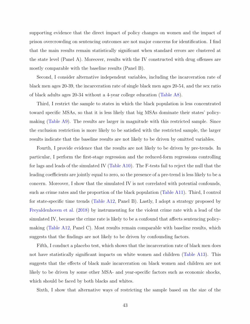
supporting evidence that the direct impact of policy changes on women and the impact of

prison overcrowding on sentencing outcomes are not major concerns for identification. I find

that the main results remain statistically significant when standard errors are clustered at

the state level (Panel A). Moreover, results with the IV constructed with drug offenses are

mostly comparable with the baseline results (Panel B).

Second, I consider alternative independent variables, including the incarceration rate of

black men ages 20-39, the incarceration rate of single black men ages 20-54, and the sex ratio

of black adults ages 20-34 without a 4-year college education (Table A8).

Third, I restrict the sample to states in which the black population is less concentrated

toward specific MSAs, so that it is less likely that big MSAs dominate their states’ policy-

making (Table A9). The results are larger in magnitude with this restricted sample. Since

the exclusion restriction is more likely to be satisfied with the restricted sample, the larger

results indicate that the baseline results are not likely to be driven by omitted variables.

Fourth, I provide evidence that the results are not likely to be driven by pre-trends. In

particular, I perform the first-stage regression and the reduced-form regressions controlling

for lags and leads of the simulated IV (Table A10). The F-tests fail to reject the null that the

leading coefficients are jointly equal to zero, so the presence of a pre-trend is less likely to be a

concern. Moreover, I show that the simulated IV is not correlated with potential confounds,

such as crime rates and the proportion of the black population (Table A11). Third, I control

for state-specific time trends (Table A12, Panel B). Lastly, I adopt a strategy proposed by

Freyaldenhoven et al. (2018) by instrumenting for the violent crime rate with a lead of the

simulated IV, because the crime rate is likely to be a confound that affects sentencing policy-

making (Table A12, Panel C). Most results remain comparable with baseline results, which

suggests that the findings are not likely to be driven by confounding factors.

Fifth, I conduct a placebo test, which shows that the incarceration rate of black men does

not have statistically significant impacts on white women and children (Table A13). This

suggests that the effects of black male incarceration on black women and children are not

likely to be driven by some other MSA- and year-specific factors such as economic shocks,

which should be faced by both blacks and whites.

Sixth, I show that alternative ways of restricting the sample based on the size of the

43

MSA black population do not affect the results (Table A14).

7 Theoretical Framework

In order to interpret the results in a more economically grounded manner, I develop a simple

three-period model in which women make consumption and marriage decisions given their

marriage market conditions, which differ by the male incarceration rate. A woman faces the

following trade-off: If she chooses not to marry now, she may not be able to meet a marriage

partner in the future; if she chooses to marry now, she can obtain financial support from

her husband now, but takes the risk that he could be incarcerated in the future, which is

harmful to the family. A detailed setup of the model is shown in Appendix A5.

Simulation of the model suggests that for a given set of beliefs about the likelihood of

meeting a partner, the likelihood of the potential spouse’s incarceration, and characteristics of

the spouse, higher incarceration rates lower the percentage of women who marry. Moreover,

women with higher asset levels (e.g., human capital) are the first to opt out of marriage.

Intuitively, when the incarceration rate is high enough, the expected cost of having a husband

incarcerated can be higher than the gain from marriage. This is more likely to be the case

for women with higher asset levels, who have higher values of being single. The simulation

evidence supports the empirical result that the incarceration of black men has a substantial

impact on more educated women.

Simulation also suggests that given an incarceration rate, the percentages of women who

choose to marry are different in different periods. This implies that women with the same

asset level can make different marriage decisions in different periods (e.g., age or life stage)

when facing the same marriage market conditions. This is because women face different

trade-offs in different periods, and therefore the likelihood of marriage should not be uniform

across ages. As a result, the empirical results should be interpreted as weighted average

effects for women of different ages.

44

8 Conclusion

This paper identifies the causal impacts of the incarceration rate of black men on black women

and children. I overcome the potential endogeneity of the incarceration rate by exploiting

plausibly exogenous changes in sentencing policies across states and over years. Specifically,

I construct a simulated IV that characterizes how sentencing policies affect incarceration

at the extensive margin, through the probability of incarceration conditional on arrest, and

at the intensive margin, through the average length of sentence served in prison. The IV

identifies the causal effects of “missing” black men at the margins of incarceration, where

the punitiveness of sentencing policies matters.

I find that rising incarceration rates of black men decrease the likelihood of marriage

for black women, and increase the likelihood of employment for those with relatively higher

education levels. For black children, rising incarceration rates of black men increase the

likelihood of being born out of wedlock and living in a mother-only family, and decrease

the likelihood of having some college education in the long run. Moreover, black boys who

grow up in areas with harsher sentencing policies tend to have lower income in adulthood

compared with white boys who grow up in the same area with similar parental income.

Finally, I find that black men at the extensive (intensive) margin of incarceration have a

larger impact on the marriage of more (less) educated women. For children, the impacts of

intensive-margin black male incarceration are especially large.

The results could be due to the declining availability of marriageable black men in the

marriage market. In particular, I find that black men without any college education are

less likely to be employed in areas with higher incarceration rates. In addition, higher

incarceration rates of black men may increase the bargaining power of black men without

criminal record. As evidence, I find that as the incarceration rate of black men increases,

black women are more likely to marry down and black men with some college education are

less likely to be married and more likely to have white wives. Finally, surging incarceration

rates of black men may also change women’s beliefs about marriage, and they may choose to

stay single if it is a better alternative to marriage. Consistently, I find that more educated

black women are less likely to be married and more likely to be employed.

45

The results have implications for sentencing policies and other correctional programs.

First, my results suggest negative impacts of black male incarceration on black women and

children. Thus, the collateral impacts of incarceration could be taken into consideration when

evaluating benefits and costs of sentencing policies. Second, my results indicate that black

men at the extensive margin of incarceration due to harsher sentencing policies have negative

impacts on black women and children. Therefore, alternative sentencing to incarceration for

those who commit less serious crimes or crimes that cause less harm to society could be more

welfare enhancing if the collateral impacts of incarceration are considered. For instance, New

York State has created a number of Alternative to Incarceration Programs to help some

offenders, particularly those with misdemeanors, without incarcerating them. Finally, my

results suggest that the negative collateral consequences of black male incarceration could fall

primarily on the poor and minorities, which could exacerbate inequality and racial gaps. For

example, a simple back-of-the-envelope calculation suggests that the average gap in income

rank between white and black men conditional on parental income could be reduced by 1

percentile, if they were exposed to the 1986 sentencing policies prior to age 23 (between

1986 and 2001). This potential consequence could also be considered when evaluating the

criminal justice system.

46

Figure 1: Estimated and Reported Prison Population(MSA Level, Black Male)

01

00

00

20

00

03

00

00

01

00

00

20

00

03

00

00

0 10000 20000 30000

0 10000 20000 30000 0 10000 20000 30000

2004 2005 2006

2007 2008

MSA prison population 45-degree line

Estim

ate

d M

SA

priso

n p

op

ula

tio

n o

f b

lack m

ale

s

Reported MSA prison population of black males

Graphs by year

Note: These figures check the consistency between NCRP Yearend Population Data and NCRP Admissionsand Releases Data. The x-axis shows the year-end prison population directly estimated from NCRP YearendPopulation Data. The y-axis shows the prison population backed out using the year-end prison populationin 2009 from Yearend Population Data, and the yearly changes in the prison population (i.e., the numberof admissions minus the number of releases within each year and MSA) from Admissions and Releases Databetween 2005 and 2009. Each point represents a MSA.

47

Figure 2: Prison Population from NCRP and NPS(State Level, Black Male)

02

04

06

00

20

40

60

02

04

06

0

1980 1990 2000 20101980 1990 2000 20101980 1990 2000 2010

California Michigan New Jersey

New York South Carolina Tennessee

Texas Virginia Wisconsin

Estimated from NCRP NPS

Priso

n p

op

ula

tio

n o

f b

lack m

ale

s (

tho

usa

nd

s)

Year

Graphs by state

Note: These figures checks the reliability of the MSA-level prison population estimated from the NCRP.The blue circles represent the state prison population obtained by aggregating the MSA prison populationestimated from the NCRP. The red x-markers represent the state prison population from the NPS. Thefigures show estimates for large states that have admission and release records going back to the 1980s. Theaverage correlation of the two estimates for all the states in my sample is 0.935.

48

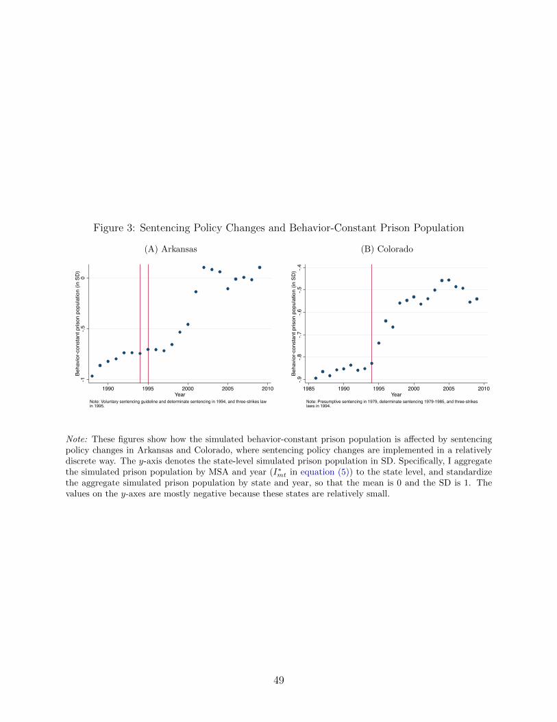
Figure 3: Sentencing Policy Changes and Behavior-Constant Prison Population

(A) Arkansas

-1-.

50

Be

ha

vio

r-co

nsta

nt p

riso

n p

op

ula

tio

n (

in S

D)

1990 1995 2000 2005 2010Year

Note: Voluntary sentencing guideline and determinate sentencing in 1994, and three-strikes lawin 1995.

(B) Colorado

-.9

-.8

-.7

-.6

-.5

-.4

Be

ha

vio

r-co

nsta

nt p

riso

n p

op

ula

tio

n (

in S

D)

1985 1990 1995 2000 2005 2010Year

Note: Presumptive sentencing in 1979, determinate sentencing 1979-1985, and three-strikeslaws in 1994.

Note: These figures show how the simulated behavior-constant prison population is affected by sentencingpolicy changes in Arkansas and Colorado, where sentencing policy changes are implemented in a relativelydiscrete way. The y-axis denotes the state-level simulated prison population in SD. Specifically, I aggregatethe simulated prison population by MSA and year (I∗mt in equation (5)) to the state level, and standardizethe aggregate simulated prison population by state and year, so that the mean is 0 and the SD is 1. Thevalues on the y-axes are mostly negative because these states are relatively small.

49

Figure 4: Number of Persons Serving Time in Prison Per 1,000 Arrests

(A) Violent Offenses

05

01

00

15

02

00

05

01

00

15

02

00

0-1 1-2 2-3 3-4 4-5 5+ 0-1 1-2 2-3 3-4 4-5 5+

Murder & Manslaughter Forcible Rape

Robbery Aggrevated Assult

Incarcerated in 1988 Incarcerated in 2000

Ad

mis

sio

ns p

er

1,0

00

Arr

ests

Years Served

Graphs by category of offenses

(B) Property Offenses

05

01

00

15

00

50

10

01

50

0-1 1-2 2-3 3-4 4-5 5+ 0-1 1-2 2-3 3-4 4-5 5+

Burglary Motor Vehicle Theft

Arson White Collar Crimes

Incarcerated in 1988 Incarcerated in 2000

Ad

mis

sio

ns p

er

1,0

00

Arr

ests

Years Served

Graphs by category of offenses

(C) Drug Offenses

05

01

00

15

0

0-1 1-2 2-3 3-4 4-5 5+ 0-1 1-2 2-3 3-4 4-5 5+

Drug Trafficking Drug Possession

Incarcerated in 1988 Incarcerated in 2000

Ad

mis

sio

ns p

er

1,0

00

Arr

ests

Years Served

Graphs by category of offenses

(D) Public Order Offenses

02

46

8

0-1 1-2 2-3 3-4 4-5 5+ 0-1 1-2 2-3 3-4 4-5 5+

Commercialized Vice Driving Under Influence

Incarcerated in 1988 Incarcerated in 2000

Ad

mis

sio

ns p

er

1,0

00

Arr

ests

Years Served

Graphs by category of offenses

Note: This figures show the number of persons per 1,000 arrests who served t years in prison for those whowere arrested in 1988 (in dotted blue lines) and in 2000 (in solid red lines) for each type of offense. t isdivided into 6 groups shown on the x-axis: 0-1 year, 1-2 years, 2-3 years, 3-4 years, 4-5 years, and 5 ormore years. The number of arrests is from the UCR. The number of admissions and the average time servedin prison are estimated from the NCRP. Estimation requires two assumptions: (1) the offense listed in theUCR data is the most serious charge against the arrestee at the time of arrest, since I use the offense of thelongest sentence from the NCRP data, and (2) the year of prison admission is same as the year of arrest. Tobe comparable with Neal and Rick (2016), the figures are obtained using admission and release records fromeight states with high data quality: California, Colorado, Michigan, New Jersey, New York, South Carolina,Washington, and Wisconsin. Neal and Rick (2016) show that the prison population patterns in these statesare comparable to those in all state.

50

Figure 5: Likelihood of Incarceration Per Arrestee(Black Adults, Drug Possession)

0.0

2.0

4.0

6.0

8.1

Lik

elih

oo

d o

f in

ca

rce

ratio

n p

er

arr

este

e

1980 1990 2000 2010Year

Note: Anti-Drug Abuse Act effective on Oct 27, 1986. Anti-Drug Abuse Amendments Act effectiveon Nov 18, 1988.

Note: This figure shows the likelihood of incarceration conditional on arrest for drug possession for blackadults. The number of arrests is from the UCR and the number of prison admissions is from the NCRP.

51

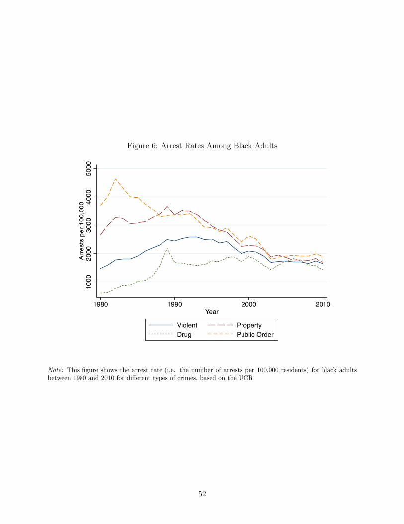
Figure 6: Arrest Rates Among Black Adults

10

00

20

00

30

00

40

00

50

00

Arr

ests

pe

r 1

00

,00

0

1980 1990 2000 2010Year

Violent Property

Drug Public Order

Note: This figure shows the arrest rate (i.e. the number of arrests per 100,000 residents) for black adultsbetween 1980 and 2010 for different types of crimes, based on the UCR.

52

Figure 7: Intergenerational Gaps in Individual Income Rankand Punitiveness of Sentencing Policies

(A) Black-White, Males, Parents at 25th Percentile

35

40

45

50

55

Me

an

ch

ild in

co

me

ra

nk (

pa

ren

ts 2

5th

)

−2 0 2 4Punitiveness of sentencing policies

White male, slope: −0.193 (0.137)

Black male, slope: −0.669 (0.127)

(B) Black-White, Males, Parents at 75th Percentile

50

55

60

65

70

Me

an

ch

ild in

co

me

ra

nk (

pa

ren

ts 7

5th

)−2 0 2 4

Punitiveness of sentencing policies

White male, slope: −0.049 (0.106)

Black male; Slope: −0.544 (0.162)

(C) Male-Female, Blacks, Parents at 25th Percentile

36

38

40

42

44

46

Me

an

ch

ild in

co

me

ra

nk (

pa

ren

ts 2

5th

)

−2 0 2 4Punitiveness of sentencing policies

Black male, slope: −0.669 (0.127)

Black female, slope: −0.076 (0.137)

(D) Male-Female, Blacks, Parents at 75th Percentile

48

50

52

54

56

58

Me

an

ch

ild in

co

me

ra

nk (

pa

ren

ts 7

5th

)

−2 0 2 4Punitiveness of sentencing policies

Black male, slope: −0.544 (0.162)

Black female, slope: 0.324 (0.164)

Note: These figures present binned scatter plots of the relationship between child individual income rankconditional on parents’ income and the punitiveness of sentencing policies across commuting zones wherechildren grow up. In each panel, the punitiveness of sentencing policies (I∗c ) is binned into 40 quantilesand plotted on the x-axis. The mean child individual income rank is plotted on the y-axis. I control forthe poverty rate in all panels. I estimate the fit lines on the binned points using OLS and report the slopecoefficients and standard errors (in parentheses).

53

Table 1: Summary Statistics for Black Men

Samples Prison Admission State Prisons Institutions Resident Pop.

Mean SD Mean SD Mean SD Mean SD(1) (2) (3) (4) (5) (6) (7) (8)

Share of ages 20-54 0.93 0.25 0.94 0.23 0.83 0.37 0.59 0.49

For black men ages 20-54Married NA NA 0.16 0.36 0.14 0.35 0.40 0.49Single NA NA 0.79 0.41 0.81 0.39 0.55 0.50Never married NA NA 0.67 0.47 0.71 0.46 0.45 0.50HS diploma 0.34 0.47 0.28 0.45 0.39 0.49 0.34 0.47Some college 0.07 0.25 0.11 0.31 0.15 0.36 0.28 0.45College degree 0.01 0.09 0.02 0.14 0.02 0.13 0.14 0.35Employed NA NA 0.67 0.47 NA NA 0.72 0.45Full-time employed NA NA 0.53 0.50 NA NA 0.61 0.49

Observations 2,460,870 20,524 37,650 1,070,933

Note: Estimates in Columns 1-2 are based on NCRP Admissions Data 1986-2009. Estimates inColumns 3-4 are based on the SISCF 1986, 1991, 1997, and 2004. Estimates in Columns 5-6 are basedon ACS 2006-2009 samples in institutions. Estimates in Columns 7-8 are based on the householddata 1986-2009. All estimates are for black men ages 20-54 (except for row 1 for all black maleadults). Variables HS diploma, Some college, and College degree are indicators for the highest levelof education.

54

Table 2: Sentencing Policy Changes

States Determinate Sentencing Guidelines Truth in Sentencingd Three-Strikes

Sentencinga Yearsb Voluntaryc Years Requirements Lawse

AlabamaAlaska 1980∗∗ 1980 No 100%Arizona 1994 1978∗∗∗ 1994 85%Arkansas∗ 1994∗∗ 1994 Yes 70% 1995California∗ 1976 1976∗∗∗ 1994 85% 1994Colorado∗ 1979-1985 1979∗∗∗ 75% 1994Connecticut 1981-1990 1994 50% 1994

1996 85%Delaware 1990 1987 Yes 1990 85%District of Col. 2000 85%Florida∗ 1983 1983 1983-1994 1995 85% 1995Geogia∗ 1995 85% 1995HawaiiIdaho 100%Illinois 1978 1995 85%Indiana 1977 1977∗∗∗ 50% 1994Iowa 1996 85%Kansas 1993 1993 No 1993 80% 1994

1995 85%Kentucky 1998 85%Louisiana∗ 1987 Yes 1997 85% 1994Maine 1976 1995 85%Maryland 1983 Yes 50% 1994Massachusetts 75%Michigan∗ 1984 1984-1999 1994 85%Minnesota∗ 1980 1980 No 1993 85%Mississippi 1995-2000 1995 85%Missouri∗ 1997 Yes 1994 85%Montana 25% 1995Nebraska 50%Nevada 100% 1995New Hampshire 1982 100%New Jersey∗ 1977∗∗∗ 1997 85% 1995New Mexico 1977 1977∗∗∗ 1994New York∗ 1995 85%North Carolina∗ 1981 1994 No 1994 85% 1994North Dakota 1995 85% 1995Ohio 1996 1996 No 1996 85%Oklahoma∗ 1998 85%Oregon∗ 1989 1989 No 1990 80%

55

1995 100%Pennsylvania∗ 1982 No 1911 85% 1995Rhode Island∗ 1981∗∗∗

South Carolina∗ 1996 1996South Dakota 85%Tennessee∗ 1989∗∗ 1989 No 1995 85% 1994Texas∗ 50%Utah 1979 Yes 1985 85% 1995Vermont 1995Virginia∗ 1995 1991 Yes 1995 85% 1994Washington∗ 1984 1984 No 1990 85% 1993West VirginiaWisconsin∗ 1999 1985-1995 Yes 1999 100% 1994Wyoming

Note: 22 states (∗) are in the sample of analysis because of data limitations of the NCRP. Details are discussedin Section 3 and Appendix A2.aYears of determinate sentencing are from Stemen et al. (2006). A range means that indeterminate sentencingreinstated later. Some states (∗∗) partially abolished parole release (Frase, 2005).bYears of sentencing guidelines are from Frase (2005). Some states (∗∗∗) adopted presumptive sentencing, asystem of single recommended terms or narrow sentence ranges (Stemen et al., 2006).cInformation on whether sentencing guidelines are voluntary is from Frase (2005) and Stemen et al. (2006). Arange means that guidelines were voluntary during the period.dYears of truth-in-sentencing laws and requirements are from Ditton and Wilson (1999) and Sabol et al. (2002).eYears of three-strikes laws are from Marvell and Moody (2001).

56

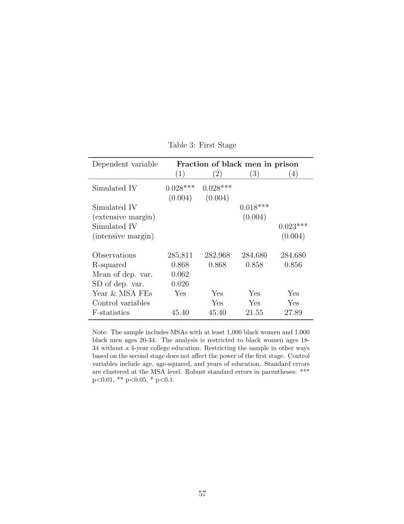
Table 3: First Stage

Dependent variable Fraction of black men in prison(1) (2) (3) (4)

Simulated IV 0.028*** 0.028***(0.004) (0.004)

Simulated IV 0.018***(extensive margin) (0.004)Simulated IV 0.023***(intensive margin) (0.004)

Observations 285,811 282,968 284,680 284,680R-squared 0.868 0.868 0.858 0.856Mean of dep. var. 0.062SD of dep. var. 0.026Year & MSA FEs Yes Yes Yes YesControl variables Yes Yes YesF-statistics 45.40 45.40 21.55 27.89

Note: The sample includes MSAs with at least 1,000 black women and 1,000black men ages 20-34. The analysis is restricted to black women ages 18-34 without a 4-year college education. Restricting the sample in other waysbased on the second stage does not affect the power of the first stage. Controlvariables include age, age-squared, and years of education. Standard errorsare clustered at the MSA level. Robust standard errors in parentheses: ***p<0.01, ** p<0.05, * p<0.1.

57

Table 4: Impact of Black Male Incarceration on the Likelihood ofBeing Married for Black Women

Dependent variable MarriedSamples Black women with some college Black women with no college

OLS 2SLS 2SLS OLS 2SLS 2SLS(1) (2) (3) (4) (5) (6)

Fraction of black -0.336 -3.192** -3.121** -0.272 -2.797** -2.640**men in prison (0.380) (1.518) (1.324) (0.352) (1.213) (1.156)

Observations 119,511 119,511 116,668 166,300 166,300 166,300R-squared 0.037 0.033 0.129 0.033 0.030 0.103Mean of dep. var. 0.238 0.193SD of dep. var. 0.426 0.395Year & MSA FEs Yes Yes Yes Yes Yes YesControl variables Yes Yes

Note: The sample includes MSAs with at least 1,000 black men and 1,000 black women ages 20-34. Columns 1-3 include black women ages 18-34 with some college education (without degrees) andColumns 4-6 include black women ages 18-34 without any college education. Control variables includeage, age-squared, and years of education. Standard errors are clustered at the MSA level. Robuststandard errors in parentheses: *** p<0.01, ** p<0.05, * p<0.1.

Table 5: Mean of Characteristics for Compliers and All Black Offenders

Compliers All Black Offenders

Age 27.73 32.38Violent offense 0.20 0.27Property offense 0.21 0.28Drug offense 0.43 0.36Public offense 0.16 0.08Prior felony 0.79 0.49

Note: The sample includes all black male offenders who wereadmitted to prison between 1986 and 2009, and whose MSAsof sentence include at least 1,000 black men and 1,000 blackwomen ages 20-34. For simplicity, I assume a binary instru-ment Zmt, where Zmt = 1 if the change in the simulated IVfor MSA m and year t (relative to 1986) is greater than themedian. Similarly, I assume a binary treatment Wmt, whereWmt = 1 if the change in the black male incarceration rate (rel-ative to 1986) is greater than the median. Define Wmt(j) to bethe potential outcome of Wmt given that Zmt = j, j ∈ {0, 1}.Therefore, compliers are prisoners who were sentenced in MSAm and year t, where Wmt(0) = 0 or Wmt(1) = 1.

58

Table 6: Impact of Black Male Incarceration on OtherMarriage Market Outcomes for Black Women

Dependent variables Never married Divorced Marry out Marry up2SLS 2SLS 2SLS 2SLS(1) (2) (3) (4)

Panel A: Impact for black women with some college

Fraction of black 2.332** 0.994 -0.489 -1.876*men in prison (0.981) (0.823) (0.470) (1.018)

Observations 116,668 116,668 116,668 116,668R-squared 0.234 0.083 0.030 0.074Mean of dep. var. 0.661 0.0984 0.0184 0.160SD of dep. var. 0.474 0.298 0.134 0.366

Panel B: Impact for black women with no college

Fraction of black 2.573** 0.274 0.114 -2.937***men in prison (1.196) (0.693) (0.254) (1.094)

Observations 166,300 166,300 166,300 166,300R-squared 0.190 0.073 0.017 0.080Mean of dep. var. 0.709 0.0918 0.0108 0.199SD of dep. var. 0.454 0.289 0.104 0.400

Year & MSA FEs Yes Yes Yes YesControl variables Yes Yes Yes Yes

Note: The sample includes MSAs with at least 1,000 black men and 1,000 black women ages20-34. The dependent variable is an indicator of being never married in Column 1, an indicatorof being divorced in Column 2, an indicator of having a non-black husband in Column 3, andan indicator of having a husband whose years of education are at least equal to the wife’s inColumn 4. Panel A includes black women ages 18-34 with some college education, and PanelB includes black women ages 18-34 without any college education. Control variables includeage, age-squared, and years of education. Standard errors are clustered at the MSA level.Robust standard errors in parentheses: *** p<0.01, ** p<0.05, * p<0.1.

59

Table 7: Impact of Black Male Incarceration on the Likelihood ofBeing Employed for Black Women

Dependent variable EmployedSamples Black women with college Black women with no college

OLS 2SLS 2SLS OLS 2SLS 2SLS(1) (2) (3) (4) (5) (6)

Fraction of black 0.404 2.883*** 2.989*** 0.487 0.748 0.821men in prison (0.424) (1.091) (1.100) (0.372) (1.394) (1.306)

Observations 138,354 138,354 135,715 116,146 116,146 116,146R-squared 0.020 0.017 0.042 0.035 0.035 0.067Mean of dep. var. 0.769 0.557SD of dep. var. 0.422 0.497Year & MSA FEs Yes Yes Yes Yes Yes YesControl variables Yes Yes

Note: The sample includes MSAs with at least 1,000 black men and 1,000 black women ages 20-34.Columns 1-3 include black women ages 22-34 with some college education or higher, and Columns4-6 include black women ages 22-34 without any college education. Control variables include age,age-squared, and years of education. Standard errors are clustered at the MSA level. Robuststandard errors in parentheses: *** p<0.01, ** p<0.05, * p<0.1.

60

Table 8: Impact of Black Male Incarceration on Black Women’s Income

Dependent variables Wage income Value of food stamps

Samples with zero without zero with zero without zero2SLS 2SLS 2SLS 2SLS(1) (2) (3) (4)

Panel A: Impact for black women with some college or higher

Fraction of black 63,985 33,966 3,001 6,413men in prison (42,589) (43,938) (2,402) (9,142)

Observations 135,715 117,429 39,533 6,726R-squared 0.198 0.246 0.066 0.112Mean of dep. var. 18600 21922 269 1957SD of dep. var. 15530 14540 840 1353

Panel B: Impact for black women with no college

Fraction of black 10,204 37,395 16,614** 15,271men in prison (27,759) (31,536) (7,247) (9,662)

Observations 116,146 78,206 31,285 12,804R-squared 0.083 0.102 0.074 0.077Mean of dep. var. 9257 13927 977.9 2554SD of dep. var. 10564 10142 1587 1597

Year & MSA FEs Yes Yes Yes YesControl variables Yes Yes Yes Yes

Note: The sample includes MSAs with at least 1,000 black men and 1,000 black womenages 20-34. The dependent variable is wage income with observations of 0 in Column1 and without observations of 0 in Column 2, and the value of food stamps receivedwith observations of 0 in Column 3 and without observations of 0 in Column 4. Top 1%observations of the dependent variables are winterized. Panel A includes black womenages 22-34 with some college education or higher and Panel B includes black womenages 22-34 with no college education. Control variables include age, age-squared, andyears of education. Standard errors are clustered at the MSA level. Robust standarderrors in parentheses: *** p<0.01, ** p<0.05, * p<0.1.

61

Table 9: Impact of Black Male Incarceration on Children’s Family Structure

Dependent variables Live with mother only Out-of-wedlock birth

OLS 2SLS 2SLS OLS 2SLS 2SLS(1) (2) (3) (4) (5) (6)

Fraction of black 0.427 3.535*** 3.533*** 0.834* 4.343*** 4.292***men in prison (0.403) (1.119) (1.119) (0.467) (1.487) (1.495)

Observations 661,425 661,425 661,425 120,778 120,778 120,778R-squared 0.020 0.017 0.018 0.038 0.034 0.035Mean of dep. var. 0.496 0.472SD of dep. var. 0.500 0.499Year & MSA FEs Yes Yes Yes Yes Yes YesControl variables Yes Yes

Note: In Columns 1-3, the depend variable is an indicator of living in a mother-only family; thesample includes MSAs with at least 2,000 black children age 0-14; the analysis is restricted toblack children ages 0-14. In Columns 4-6, the depend variable is an indicator that mother is nevermarried; the sample includes MSAs with at least 2,000 black children age 0-14; the analysis isrestricted to black infants. Control variables include age and gender. Standard errors are clusteredat the MSA level. Robust standard errors in parentheses: *** p<0.01, ** p<0.05, * p<0.1.

Table 10: Long-Run Impact of Black Male Incarceration onBlack Children’s Educational Outcome

Dependent variable Have at least one-year collegeSamples Black men 22-24 Black women 22-24

OLS 2SLS 2SLS OLS 2SLS 2SLS(1) (2) (3) (4) (5) (6)

Mean fraction of black men -1.123** -4.432** -3.897** -0.749 -3.216** -3.185**in prison in early adolescence (0.449) (2.221) (1.926) (0.531) (1.639) (1.522)

Observations 19,326 19,326 13,571 23,975 23,975 17,242R-squared 0.043 0.040 0.050 0.041 0.040 0.043Mean of dep. var. 0.434 0.434 0.394 0.524 0.524 0.495SD of dep. var. 0.496 0.496 0.489 0.499 0.499 0.500Year & MSA FEs Yes Yes Yes Yes Yes Yes

Note: Columns 1-3 include black men ages 22-24. Columns 4-6 include black women ages 22-24. Columns 3and 6 further restrict the sample to individuals whose state of birth is same as the current state of residence.Standard errors are clustered at the MSA level. Robust standard errors in parentheses: *** p<0.01, **p<0.05, * p<0.1.

62

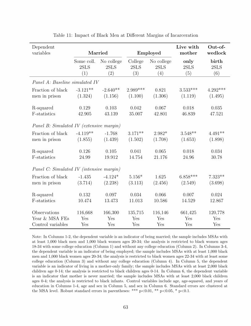
Table 11: Impact of Black Men at Different Margins of Incarceration

Dependent Live with Out-of-variables Married Employed mother wedlock

Some coll. No college College No college only birth2SLS 2SLS 2SLS 2SLS 2SLS 2SLS(1) (2) (3) (4) (5) (6)

Panel A: Baseline simulated IV

Fraction of black -3.121** -2.640** 2.989*** 0.821 3.533*** 4.292***men in prison (1.324) (1.156) (1.100) (1.306) (1.119) (1.495)

R-squared 0.129 0.103 0.042 0.067 0.018 0.035F-statistics 42.905 43.139 35.007 42.801 46.839 47.521

Panel B: Simulated IV (extensive margin)

Fraction of black -4.119** -1.768 3.171** 2.982* 3.548** 4.491**men in prison (1.855) (1.439) (1.502) (1.708) (1.653) (1.898)

R-squared 0.126 0.105 0.041 0.065 0.018 0.034F-statistics 24.99 19.912 14.754 21.176 24.96 30.78

Panel C: Simulated IV (intensive margin)

Fraction of black -1.435 -4.124* 5.156* 1.625 6.858*** 7.323**men in prison (3.714) (2.238) (3.113) (2.456) (2.549) (3.698)

R-squared 0.132 0.097 0.034 0.066 0.007 0.024F-statistics 10.474 13.473 11.013 10.586 14.529 12.867

Observations 116,668 166,300 135,715 116,146 661,425 120,778Year & MSA FEs Yes Yes Yes Yes Yes YesControl variables Yes Yes Yes Yes Yes Yes

Note: In Columns 1-2, the dependent variable is an indicator of being married; the sample includes MSAs withat least 1,000 black men and 1,000 black women ages 20-34; the analysis is restricted to black women ages18-34 with some college education (Column 1) and without any college education (Column 2). In Columns 3-4,the dependent variable is an indicator of being employed; the sample includes MSAs with at least 1,000 blackmen and 1,000 black women ages 20-34; the analysis is restricted to black women ages 22-34 with at least somecollege education (Column 3) and without any college education (Column 4). In Column 5, the dependentvariable is an indicator of living in a mother-only family; the sample includes MSAs with at least 2,000 blackchildren age 0-14; the analysis is restricted to black children ages 0-14. In Column 6, the dependent variableis an indicator that mother is never married; the sample includes MSAs with at least 2,000 black childrenages 0-4; the analysis is restricted to black infants. Control variables include age, age-squared, and years ofeducation in Columns 1-4, age and sex in Column 5, and sex in Column 6. Standard errors are clustered atthe MSA level. Robust standard errors in parentheses: *** p<0.01, ** p<0.05, * p<0.1.

63

Table 12: Impact of Punitiveness of Sentencing Policies onIntergenerational Income Gap

Dependent variable Difference between white andblack men’s income rank

Parents at 25th percentile Parents at 75th percentileOLS OLS OLS OLS(1) (2) (3) (4)

Punitiveness of 0.614*** 0.619*** 0.698*** 0.709***sentencing policies (0.140) (0.139) (0.166) (0.166)Poverty rate -12.06*** -9.016**

(3.379) (4.035)

Observations 517 517 517 517R-squared 0.035 0.058 0.033 0.042Mean of dep. var. 10.273 11.392SD of dep. var. 3.221 3.851

Dependent variable Difference between black womenand men’s income rank

Parents at 25th percentile Parents at 75th percentileOLS OLS OLS OLS(1) (2) (3) (4)

Punitiveness of 0.578*** 0.601*** 0.887*** 0.901***sentencing policies (0.146) (0.142) (0.213) (0.213)Poverty rate -19.046*** -11.303**

(3.442) (5.168)

Observations 506 506 506 506R-squared 0.03 0.086 0.033 0.042Mean of dep. var. 2.486 0.283SD of dep. var. 3.317 4.9

Note: The sample includes all CZs. Standard errors are clustered at the state level.Robust standard errors in parentheses: *** p<0.01, ** p<0.05, * p<0.1.

64

References

Abramitzky, Ran, Adeline Delavande, and Luis Vasconcelos (2011), “Marrying up: The role

of sex ratio in assortative matching.” American Economic Journal: Applied Economics,

3, 124–57.

Abuse, Substance (2014), “Mental Health Services Administration (SAMHSA)(2014) Results

from the 2013 national survey on drug use and health: Summary of national findings.”

Substance Abuse and Mental Health Services Administration, Rockville, MD.

Ackerman, Jeffrey M and D Kim Rossmo (2015), “How far to travel? A multilevel analysis

of the residence-to-crime distance.” Journal of Quantitative Criminology, 31, 237–262.

Aizer, Anna and Joseph J Doyle Jr (2015), “Juvenile incarceration, human capital, and future

crime: Evidence from randomly assigned judges.” The Quarterly Journal of Economics,

130, 759–803.

Alexander, Michelle (2012), The new Jim Crow: Mass incarceration in the age of colorblind-

ness. The New Press.

Anderman, Eric M and Carol Midgley (1997), “Changes in achievement goal orientations,

perceived academic competence, and grades across the transition to middle-level schools.”

Contemporary Educational Psychology, 22, 269–298.

Andersen, Lars H (2016), “How children’s educational outcomes and criminality vary by du-

ration and frequency of paternal incarceration.” The ANNALS of the American Academy

of Political and Social Science, 665, 149–170.

Angrist, Josh (2002), “How do sex ratios affect marriage and labor markets? Evidence from

America’s second generation.” The Quarterly Journal of Economics, 117, 997–1038.

Aughinbaugh, Alison, Omar Robles, and Hugette Sun (2013), “Marriage and divorce: Pat-

terns by gender, race, and educational attainment.” Monthly Lab. Rev., 136, 1.

65

Balfanz, Robert, Liza Herzog, and Douglas J Mac Iver (2007), “Preventing student disen-

gagement and keeping students on the graduation path in urban middle-grades schools:

Early identification and effective interventions.” Educational Psychologist, 42, 223–235.

Banks, Ralph Richard (2011), Is marriage for white people?: How the African American

marriage decline affects everyone. Penguin.

Beck, Allen J, Jennifer C Karberg, and Paige M Harrison (2002), “Prison and jail inmates

at midyear 2001.” Bureau of Justice Statistics Bulletin, 1.

Becker, Gary S (1968), “Crime and punishment: An economic approach.” In The economic

dimensions of crime, 13–68, Springer.

Becker, Gary S (1973), “A theory of marriage: Part I.” Journal of Political economy, 81,

813–846.

Becker, Gary S (1974), “A theory of marriage: Part II.” Journal of political Economy, 82,

S11–S26.

Becker, Gary S, Elisabeth M Landes, and Robert T Michael (1977), “An economic analysis

of marital instability.” Journal of political Economy, 85, 1141–1187.

Blumstein, Alfred and Allen J Beck (1999), “Population growth in US prisons, 1980-1996.”

Crime and justice, 26, 17–61.

Bonczar, Thomas P (2003), “Prevalence of imprisonment in the US population, 1974-2001.”

Brainerd, Elizabeth (2017), “The lasting effect of sex ratio imbalance on marriage and family:

Evidence from World War II in Russia.” Review of Economics and Statistics, 99, 229–242.

Caucutt, Elizabeth M, Nezih Guner, and Christopher Rauh (2016), “Is marriage for white

people? Incarceration and the racial marriage divide.”

Centers for Disease Control and Prevention (2018), “CDC Wonder: Bridged-race population

estimates 2001.” URL https://wonder.cdc.gov/bridged-race-population.html.

Champion, Dean J (2008), Sentencing: A Reference Handbook. Abc-clio.

66

Charles, Kerwin Kofi and Ming Ching Luoh (2010), “Male incarceration, the marriage mar-

ket, and female outcomes.” The Review of Economics and Statistics, 92, 614–627.

Chetty, Raj and Nathaniel Hendren (2018), “The impacts of neighborhoods on intergenera-

tional mobility I: Childhood exposure effects.” The Quarterly Journal of Economics, 133,

1107–1162.

Chetty, Raj, Nathaniel Hendren, Maggie R Jones, and Sonya R Porter (2018), “Race and

economic opportunity in the United States: An intergenerational perspective.” Technical

report, National Bureau of Economic Research.

Chiappori, Pierre-Andre, Bernard Fortin, and Guy Lacroix (2002), “Marriage market, di-

vorce legislation, and household labor supply.” Journal of political Economy, 110, 37–72.

Clark, John, James Austin, and D Alan Henry (1997), “Three Strikes and You’re Out”:

A Review of State Legislation. US Department of Justice, Office of Justice Programs,

National Institute of Justice.

Clear, Todd R (2008), “The effects of high imprisonment rates on communities.” Crime and

Justice, 37, 97–132.

Cox, Oliver C (1940), “Sex ratio and marital status among Negroes.” American sociological

review, 5, 937–947.

Currie, Janet and Jonathan Gruber (1996), “Health insurance eligibility, utilization of med-

ical care, and child health.” The Quarterly Journal of Economics, 111, 431–466.

Derenoncourt, Ellora (2018), “Can you move to opportunity? Evidence from the Great

Migration.”

Ditton, Paula M and Doris James Wilson (1999), Truth in sentencing in state prisons. US

Department of Justice, Office of Justice Programs, Bureau of Justice Statistics Washing-

ton, DC.

Donohue III, John J and Steven D Levitt (2001), “The impact of race on policing and

arrests.” The Journal of Law and Economics, 44, 367–394.

67

Easterlin, Richard A. (1961), “The American baby boom in historical perspective.”

The American Economic Review, 51, 869–911, URL http://www.jstor.org/stable/

1813841.

Flood, Sarah, Miriam King, Steven Ruggles, and J. Robert Warren (2017), “Integrated Pub-

lic Use Microdata Series, Current Population Survey: Version 5.0. [dataset].” Minneapolis:

University of Minnesota, URL https://doi.org/10.18128/D030.V5.0.

Frase, Richard S (2005), “State sentencing guidelines: Diversity, consensus, and unresolved

policy issues.” Colum. L. Rev., 105, 1190.

Freyaldenhoven, Simon, Christian Hansen, and Jesse M Shapiro (2018), “Pre-event trends in

the panel event-study design.” Technical report, National Bureau of Economic Research.

Grob, Gerald N (2000), “Mental health policy in 20th-century America.” AUTHOR Mander-

scheid, Ronald W., Ed.; Henderson, Marilyn J., Ed. TITLE Mental Health, United States,

2000. INSTITUTION Substance Abuse and Mental Health Services Administration, 18.

Gruber, Jon and Emmanuel Saez (2002), “The elasticity of taxable income: Evidence and

implications.” Journal of public Economics, 84, 1–32.

Guttentag, Marcia and Paul F Secord (1983), “Too many women? The sex ratio question.”

Johnson, Rucker C and Steven Raphael (2009), “The effects of male incarceration dynamics

on acquired immune deficiency syndrome infection rates among African American women

and men.” The Journal of Law and Economics, 52, 251–293.

Kalmijn, Matthijs (1998), “Intermarriage and homogamy: Causes, patterns, trends.” Annual

review of sociology, 24, 395–421.

Kuziemko, Ilyana and Steven D Levitt (2004), “An empirical analysis of imprisoning drug

offenders.” Journal of Public Economics, 88, 2043–2066.

Lafortune, Jeanne (2013), “Making yourself attractive: Pre-marital investments and the

returns to education in the marriage market.” American Economic Journal: Applied Eco-

nomics, 5, 151–78.

68

Laumann, Edward O., John H. Gagnon, Robert T. Michael, and Stuart Michaels (1992),

“National Health and Social Life Survey, 1992: [United States].” Ann Arbor, MI: Inter-

university Consortium for Political and Social Research [distributor], URL https://doi.

org/10.3886/ICPSR06647.v2.

Levitt, Steven D (1996), “The effect of prison population size on crime rates: Evidence from

prison overcrowding litigation.” The quarterly journal of economics, 111, 319–351.

Levitt, Steven D (2004), “Understanding why crime fell in the 1990s: Four factors that

explain the decline and six that do not.” Journal of Economic perspectives, 18, 163–190.

Marvell, Thomas B and Carlisle E Moody (2001), “The lethal effects of three-strikes laws.”

The Journal of Legal Studies, 30, 89–106.

Massoglia, Michael, Brianna Remster, and Ryan D King (2011), “Stigma or separation?

Understanding the incarceration-divorce relationship.” Social Forces, 90, 133–155.

Mechoulan, Stephane (2011), “The external effects of black male incarceration on black

females.” Journal of Labor Economics, 29, 1–35.

Mueller-Smith, Michael (2015), “The criminal and labor market impacts of incarceration.”

Unpublished Working Paper.

Neal, Derek and Armin Rick (2016), “The prison boom and sentencing policy.” The Journal

of Legal Studies, 45, 1–41.

Nicholson-Crotty, Sean (2004), “The impact of sentencing guidelines on state-level sanctions:

An analysis over time.” Crime & Delinquency, 50, 395–411.

Pager, Devah (2003), “The mark of a criminal record.” American journal of sociology, 108,

937–975.

Passel, Jeffrey S, Wendy Wang, and Paul Taylor (2010), “One-in-seven new US marriages is

interracial or interethnic.” Pew Social & Demographic Trends.

69

Pfaff, John F (2011), “The myths and realities of correctional severity: Evidence from the

national corrections reporting program on sentencing practices.” American Law and Eco-

nomics Review, 13, 491–531.

Raphael, Steven and Michael A Stoll (2013), Why are so many Americans in prison? Russell

Sage Foundation.

Rodrigue, Edward and Richard Reeves (2015), “Single black female BA seeks educated

husband: Race, assortative mating and inequality.” Brookings Institution, 8, 1–6.

Ruggles, Steven, Katie Genadek, Ronald Goeken, Josiah Grover, and Matthew Sobek (2017),

“Integrated Public Use Microdata Series: Version 7.0 [dataset].” Minneapolis: University

of Minnesota, URL https://doi.org/10.18128/D010.V7.0.

Sabol, William J et al. (2002), “The influences of truth-in-sentencing reforms on changes in

states’ sentencing practices and prison populations.”

Stemen, Don, Andres Rengifo, and James Wilson (2006), “Of fragmentation and ferment:

The impact of state sentencing policies on incarceration rates, 1975–2002.” Final Report

to the US Department of Justice by the Vera Institute of Justice, 1–217.

Stemen, Don and Andres F Rengifo (2011), “Policies and imprisonment: The impact of

structured sentencing and determinate sentencing on state incarceration rates, 1978–2004.”

Justice Quarterly, 28, 174–201.

Tonry, Michael (2013), “Sentencing in America, 1975–2025.” Crime and Justice, 42, 141–

198.

United States Department of Justice. Federal Bureau of Investigation (1983-2009), “Uni-

form crime reporting program data: Arrests by age, sex, and race, summarized yearly,

1983-2009.” Ann Arbor, MI: Inter-university Consortium for Political and Social Research

[distributor], URL https://doi.org/10.3886/ICPSR30762.v1.

United States Department of Justice. Office of Justice Programs. Bureau of Justice Statistics

(1983-2009), “National corrections reporting program, 1983-2009.” Ann Arbor, MI: Inter-

70

university Consortium for Political and Social Research [distributor], URL https://doi.

org/10.3886/ICPSR30799.v2.

United States Department of Justice. Office of Justice Programs. Bureau of Justice Statistics

(1993), “Survey of inmates of state correctional facilities, 1991: [united states].” Ann

Arbor, MI: Inter-university Consortium for Political and Social Research [distributor],

URL https://doi.org/10.3886/ICPSR06068.v1.

United States Department of Justice. Office of Justice Programs. Bureau of Justice Statistics

(2005), “Survey of inmates of state correctional facilities, 1986: [united states].” Ann

Arbor, MI: Inter-university Consortium for Political and Social Research [distributor],

URL https://doi.org/10.3886/ICPSR08711.v2.

United States Department of Justice. Office of Justice Programs. Bureau of Justice Statistics

(2013), “National prisoner statistics, 1978-2011.” Ann Arbor, MI: Inter-university Con-

sortium for Political and Social Research [distributor], URL https://doi.org/10.3886/

ICPSR34540.v1.

United States Department of Justice. Office of Justice Programs. Bureau of Justice Statis-

tics (2018), “Survey of inmates in state and federal correctional facilities, 2004.” Ann

Arbor, MI: Inter-university Consortium for Political and Social Research [distributor],

URL https://doi.org/10.3886/ICPSR04572.v3.

United States Department of Justice. Office of Justice Programs. Bureau of Justice Statistics,

and United States Department of Justice. Federal Bureau of Prisons (2006), “Survey of

inmates in state and federal correctional facilities, 1997.” Ann Arbor, MI: Inter-university

Consortium for Political and Social Research [distributor], URL https://doi.org/10.

3886/ICPSR02598.v1.

Van der Klaauw, Wilbert (1996), “Female labour supply and marital status decisions: A

life-cycle model.” The Review of Economic Studies, 63, 199–235.

Visher, Christy Ann, Sara Debus, and Jennifer Yahner (2008), Employment after prison:

71

A longitudinal study of releases in three states. Urban Institute, Justice Policy Center

Washington, DC.

Western, Bruce (2002), “The impact of incarceration on wage mobility and inequality.”

American sociological review, 526–546.

Western, Bruce and Leonard Lopoo (2004), “Incarceration, marriage, and family life.”

Princeton University, Department of Sociology (paper).

Western, Bruce and Sara McClanahan (2000), “Fathers behind bars: The impact of incar-

ceration on family formation.”

Wildeman, Christopher and Christopher Muller (2012), “Mass imprisonment and inequality

in health and family life.” Annual Review of Law and Social Science, 8, 11–30.

Zhang, Yan, Christopher D Maxwell, and Michael S Vaughn (2009), “The impact of state

sentencing policies on the US prison population.” Journal of Criminal Justice, 37, 190–

199.

72

Appendix

A1 Extended Literature Review

This paper is most related to Charles and Luoh (2010) and Mechoulan (2011), who estimate

the impact of male incarceration on female outcomes. Charles and Luoh (2010) study the

impact of male incarceration on women’s marriage and labor market outcomes, using de-

cennial census data from IPUMS from 1970 to 2000. The census data specify observations

in institution. The authors define a marriage market by the interaction of race, age group,

and state, and exploit variation in the incarceration rates across different marriage markets

using a fixed effect model. Their identification assumptions include that (1) marriages oc-

cur within the specific race, age, and regional cells, (2) variation in the incarceration rates

comes from shocks that are exogenous to women’s marriage and labor market outcomes,

and (3) marriage markets of the whites are viable control groups for marriage markets of

the blacks. Although variation in the incarceration rates is likely to come from sentencing

policy changes to a large extent, it can still be correlated with other unobserved changes in

confounds within each marriage market over time, which may affect women’s marriage and

labor supply decisions independently. In addition, marriage markets of the whites may not

be proper control groups for marriage markets of the blacks. Charles and Luoh (2010) also

instrument for changes in the incarceration rates between 2000 and 1980 using average drug

caseloads between 1990 and 2000, using a first difference approach (because of data limita-

tion on drug caseloads in early years). However, drug caseloads do not plausibly satisfy the

exclusion restriction. For instance, drug caseloads can be correlated with prevalence of illicit

drugs or police discrimination, which can affect women’s marriage decisions independently.

Furthermore, women may not want to marry a man who is addicted to drugs. Mechoulan

(2011) differs from Charles and Luoh (2010) by using prisoner statistics (1978-2003) from the

Bureau of Justice Statistics (BJS) and annual household data from the Current Population

Survey (CPS). In addition, the author controls for state-specific time trends. However, the

estimates may still not represent causal relationships because of omitted variables within

states and over years.

73

Results from these two studies are mixed. In general, my OLS estimates of the impact of

black male incarceration on women’s marriage and employment are comparable with those of

either Charles and Luoh (2010) or Mechoulan (2011), but the OLS estimates are substantially

smaller in magnitude than my 2SLS estimates. As to the impact on women’s marriage, the

OLS estimate with the fixed effect model of Charles and Luoh (2010) suggests that a 1 pp

increase in the male incarceration rate increases women’s likelihood of being never married by

1.1 pp (for women of all education levels). Their OLS estimate with the first difference model

is much smaller than the OLS estimate with the fixed effect model, and their 2SLS estimate

with the first difference model is similar to the OLS estimate with the fixed effect model.

Mechoulan (2011) does not find a statistically significant impact on women’s marriage. My

OLS results are similar to that of Charles and Luoh (2010): I find that a 1 pp increase

in the incarceration rate of black men increases the likelihood of being never married by

1.1 pp (0.45 pp) for black women at the state level (MSA level).74 Differences between my

state-level and MSA-level OLS estimates can be driven by measurement error. Nevertheless,

the OLS estimates are considerably smaller than my 2SLS estimates (Table 4 and Table 6).

In terms of the impact on women’s employment, Charles and Luoh (2010) find that a 1

pp increase in the male incarceration rate increases women’s likelihood of being employed by

0.6 pp with the fixed effect model, 0.4 pp with the first difference model, and 0.3 pp with the

first difference model and instrument. My OLS estimates at both the state and MSA level

show that a 1 pp increase in the incarceration rate of black men increases the likelihood of

being employed for black women by 0.4 pp. Again, the OLS estimates are much smaller than

my 2SLS estimates (Table 7). Mechoulan (2011) focuses on the impact on the likelihood

of being full-time employed for black women ages 20-22. He does not find a statistically

significant impact without state-specific time trend, and finds that a 1 pp increase in the

incarceration rate of black men increases the likelihood of being employed for black women

by 3.5 pp with state-specific time trend. Restricting my sample to black women ages 20-22,

I find an impact of 0.96 pp without controlling for state-specific time trend and an impact

of 1.54 pp with state-specific time trend. In general, my main results do not change with or

74I perform OLS regressions with state-level incarceration rates to compare with the literature. The resultsare not presented in the paper.

74

without including state-specific time trends (Table A12).

A2 National Corrections Reporting Program

A2.1 Data Description

The National Corrections Reporting Program (NCRP) data are restricted-access data from

the Bureau of Justice Statistics. They provide detailed information on persons admitted to

prison or released from prison from 1983 to 2009. Since 2004, some states also started to

provide information on inmates in custody at year end. These different types of records are

reported in different data files for each year, including the Admissions Data, the Releases

Data, and the Yearend Population Data.

The NCRP data include all the inmates who were sentenced to State or Federal prison.

Those who were sentenced to State prison but were serving time in local jails or other

facilities such as hospitals were also included in the sample. The data provide the state of

custody, the state of jurisdiction, and the county where a person was sentenced.

The NCRP data provide detailed individual demographic information in all the records,

including the date of birth, gender, race, Hispanic origin, and educational attainment. Since

my analysis mainly focuses on the incarceration of the black male, I need a clear definition of

race. The Uniform Crime Reports (UCR) arrest data report arrests by race (White, Black,

Indian, and Asian) and by Hispanic origin (Hispanic and non-Hispanic) separately, without

an interaction between race and Hispanic origin (such as non-Hispanic Black). Therefore,

to be consistent with the UCR, I consider black inmates to be those whose race is Black,

regardless of the Hispanic origin. It should be noted that before 1999, more than 60% of

prisoners with Hispanic origin reported their race as White and more than 36% had their

race missing. Since 1999, the NCRP introduced an additional race category, Other. Since

then, more than 56% of prisoners with Hispanic origin reported their race as Other, and

around 23% reported as White and another 20% had missing race information. Therefore,

to be consistent over time, I treat all the prisoners with Hispanic origin as White, unless

75

they explicitly reported their race75.

The NCRP data provide detailed categories for offenses. To estimate the probability of

being admitted to prison conditional on being arrested, I collapse the offenses into 20 broader

categories to be consistent with the UCR arrest data, including murder and manslaughter,

forcible rape, robbery, aggravated assault, other assaults, other sex offenses (not forcible or

prostitution), burglary, larceny theft, motor vehicle theft, arson, white collar crimes (includ-

ing forgery, fraud, embezzlement, stolen property possession), vandalism, weapon crimes,

commercialized vice (including prostitution and gambling), drug sale or manufacture, drug

possession, offenses against family and children, driving under the influence, liquor laws, and

drunkenness/ disorderly conduct/ vagrancy. However, I use much more detailed categories

of offenses when I estimate the average length of time served in prison so that it is more

likely to capture changes in punitiveness of sentencing policies instead of changes in severity

of crimes.

A2.2 Data Cleansing

To estimate the year-end prison population before 2004 at the level of metropolitan statistical

area (MSA), I have to obtain the year-end prison population in 2004 or afterward and yearly

admissions and releases at the MSA level. Table A1 shows states that have the NCRP

Yearend Population Data for at least one year between 2004 and 2009. The year-end prison

population before 2004 can be ONLY estimated for these states.

For each year and MSA where sentence was imposed, I calculate the number of offenders

admitted to prison and released from prison by race and gender. However, some states did

not report admissions or releases for some years. In addition, for each year of admission t, I

calculate the total number of prisoners released after t who were admitted to prison in year

t using the release records. In principle, the total number of prisoners released for a specific

year of admission should be no greater than the number of prisoners admitted in that year

calculated using the admission records. However, this is not the case for some states, in

particular in the early years. This is probably because the data quality is relatively lower in

the early years of the program and states are likely to have under-reporting of admissions

75This definition is consistent with Neal and Rick (2016).

76

and releases in the early years. The under-reporting of admissions from the early years,

however, can be reflected from the release records of later years. I follow the following

procedures to clean the records by imputing some missing records or records with evidence

of under-reporting.

1. Some states did not report regularly and some states reported unreasonably small

numbers of admissions and releases in the early years of the program. Therefore, I

delete the missing and unreliable records of the early years for each state. Table A1

column 3 shows the time periods during which the admission and release records were

regularly submitted for each state.

2. For some states, the admission and release records are missing for a few years. I imput

the missing records using records of the two closest years, assuming equal increments.

3. For some states and some year t, the total number of released prisoners who were

admitted to prisoner in year t is greater than the number of prisoners admitted to

prison in year t. This shows that the state is likely to have the issue of under-reporting

in year t. I calculate a rate of under-reporting for admissions based on the total

number of released prisoners who were admitted to prisoner in year t, which should be

a lower bound for the number of admissions in year t. Assuming that the rate of under-

reporting is the same for admissions and releases, I modify the number of prisoners

admitted to prison in year t and the number of prisoners released from prison in year

t based on the rate of under-reporting.

I calculate the year-end prison population before 2004 using the modified admission and

release records, as well as the reported year-end prison population in 2004 or afterward.

A2.3 Perpetual Inventory Method

I use the perpetual inventory method to estimate the number of prisoners by year, MSA,

race, and gender between 1986 and 2009. Let Irsmt be the number of persons incarcerated of

race r and sex s, sentenced from MSA m at year end t. Let Arsmt and Rrsmt be the number

of persons admitted to prison and released from prison, of race r and sex s, sentenced from

77

MSA m in year t, respectively. In particular, I assume that if a person was sentence in MSA

m, then he or she will return the MSA after being released. Arsmt and Rrsmt can be calculated

with the Admissions Data and the Releases Data from the NCRP. The change in the number

of persons incarcerated between year end t and year end t− 1 is

∆Irsmt = Arsmt −Rrsmt.

Therefore, I can retrieve the number of persons incarcerated at year end using the number

of persons in custody at year end 2004 or afterward, and yearly changes in the number of

persons incarcerated:

Irsm,2008 = Irsm,2009 −∆Irsm,2009

Irsm,2007 = Irsm,2008 −∆Irsm,2008

......

Irsm,1983 = Irsm,1984 −∆Irsm,1984,

where Irsmt, t ∈ {2004, ..., 2009} and ∆Irsmt, t ∈ {1983, ...., 2009} can be estimated from the

NCRP data directly.

Prison population is estimated using all observations of black male offenders greater or

equal to 18 years old from the NCRP. I do not furthermore restrict ages for estimation for

three reasons: (1) limiting ages may introduce more errors – missing or wrong reports for the

year of birth variable may lead to loss of observations or inaccurate estimation; (2) public-

data on prisoners don’t have information on the number of prisoners by year, state and age

group, so I can’t compare my estimates with reports from aggregated public-available data;

and (3) I rely on flows of prisoners to back out the year-end prison population, which makes

it hard to estimate the year-end population of a specific age group.

78

A3 More Details on Measurement

A3.1 Incarceration Rate of Single Black Men

The incarceration rate of single black men for each year t and MSA of sentence m is estimated

as follows:

Frac. of single black men in prison =# of single black men in prison

resident pop. of single black men ages 20-54. (8)

The numerator is estimated by multiplying the number of black men who are in prison in

year t sentenced from MSA m, and the share of black male inmates ages 20-54 who are

single (estimated from the SISCF and ACS). The SISCF (ACS) provides age, gender, race,

and marital status of individuals in state prisons (institutions), which allow me to estimate

the share of black men ages 20-54 in state prisons (institutions) who are single (i.e. never

married, divorced, or widowed). Unfortunately, the SISCF only provides the region (not

state) where an inmate was interviewed. Therefore, the single rate is estimated at the region

level from the SISCF and at the state level from the ACS.76 Moreover, I cannot estimate

the single rate for each year between 1986 and 2009, with data available for 1986, 1991,

1997, 2004, and 2006-2009 only. Therefore, I approximate the single rate in each year with

the number in the closest available year. The denominator is estimated by multiplying the

resident population of black men ages 20-54 and the share of black men ages 20-54 who are

single (estimated from the household data by year and state).77

A3.2 Probability of Incarceration Given Arrest

One key variable used to construct the simulated IV is the probability of incarceration given

arrest, γcs(m)t. I estimate γcs(m)t using the number of black adults admitted to prison (from the

NCRP) divided by the number of black adults arrested (from the UCR) for each category

of offense, state, and year. First, although the NCRP data provide detailed categories of

76Although the ACS provides the MSA of residence, the single rate is estimated at the state level usingthe ACS. This is because the MSA only reflects where state prisons are located, and does not reflect whereprisoners come from. Therefore, exploiting variation across MSAs is not informative.

77Although household data provide the MSA of residence, the single rate is estimated at the state level.This is because the sample size of black men ages 20-54 is very small in many MSAs, which leads to largemeasurement error.

79

offenses, the UCR arrest data only provide 43 categories of offenses. Therefore, I collapse

the offenses in each data source into 20 broader categories that can be matched with each

other. Since both datasets have reporting errors, employing broader categories can mitigate

the problem of measurement error in the matching process. In addition, although the UCR

data provide the county where a police agency locates, I estimate the variable γcs(m)t at the

state level instead of at the MSA level for two reasons. First, the UCR relies on the reports

of participating law enforcement agencies, so missing reports from some law enforcement

agencies can have a big impact on the number of arrests of a county or a MSA. Second,

the number of arrests at the MSA level is not an accurate measurement of the MSA’s crime

activities, since it is likely for offenders to commit crimes and get arrested at different places.

Finally, the UCR data do not provide the number of arrests by race and gender directly; they

only provide the number of arrests by race and by gender separately. Therefore, I use γcs(m)t

for black adults as an approximate of that for black male adults. Estimating the number of

arrested black men using the number of arrested black adults, adjusted by the share of male

arrests among the adult arrests of all races do not change the results.

A3.3 Variables for the Analysis in Section 6.6

Chetty et al. (2018) characterize the mean income ranks of children who grow up in CZ c

conditional on their parents’ ranks by regressing the children’s individual income ranks when

they are between the ages of 31 and 37 (yi,c) on their parents’ income ranks (yi,p):

yi,c = αcrs + βcrsyi,p + εi,

weighing by the number of years that child i is observed below age 23 in CZ c. Therefore,

the mean individual income rank of children of race r (r = b, w) sex s (s = m, f) who grow

up in CZ c with parents at the pth percentile of the national household income distribution

is given by

ycrsp = αcrs +p

100βcrs. (9)

They provide statistics on ycrs25 and ycrs75 on the Equality of Opportunity Project website.78

78Link: http://www.equality-of-opportunity.org/data/. Online Data Table 4 of Chetty et al. (2018).

80

To merge with ycrs25 and ycrs75 , I re-construct the measure of punitiveness of sentencing

policies at the CZ level (I∗ct) according to equation (5):

I∗ct =N∑

crime=1

γcrimes(c)t +N∑

crime=1

t−1∑j=1

γcs(c)j1{Scrime−cj > t− j}.79

Since Chetty et al. (2018) only provide ycrs25 and ycrs75 across CZs, not over time, I measure

the mean punitiveness of sentencing policies of each CZ where children in their sample grow

up with∑2001

t=1986 I∗ct, weighting by the CZ black population below age 25. Using the average

between 1986 and 2001 is because the sample of Chetty et al. (2018) consists of all children in

the 1978-83 birth cohorts, and ycrsp is constructed by assigning children to CZs in proportion

to years they spend below age 23 in each CZ. Since the NCRP data on admissions and

releases are either unavailable or unreliable before 1986, I start with the year of 1986 in the

construction. Moreover, using the average of I∗ct between 1986 and 2001 (when the 1978

cohort gets age 22) or the average of I∗ct between 1986 and 2005 (when the 1983 cohort gets

age 22) does not affect the results. The weight is the CZ black population below age 25 since

the Census U.S. Intercensal County Population Data only provide population by age group

of 5 years. At last, I standardize the measure so that the mean is zero and the standard

deviation is one across CZs (weighting by the CZ population), denoted by I∗c , with higher

values representing harsher sentencing policies.

A4 Additional Results

A4.1 Heterogeneous Effects and Potential Mechanisms

To examine the potential mechanisms behind my results, I explore heterogeneity in the

treatment effects across observable characteristics of women and conduct additional analyses.

First, I estimate differential effects of black male incarceration on black women of different

levels of education and age groups (Table A4). Panel A shows that the impact of black male

incarceration on the likelihood of marriage is larger for women of older cohorts among those

with some college education (Column 2), and larger for women of younger cohorts among

79I re-label m (MSA) with c (CZ), and c (crime) with crime to avoid ambiguity.

81

those without any college education (Column 3). Since generally college-educated people

are more likely to marry at older ages compared with their counterparts with fewer years

of education (Aughinbaugh et al., 2013), more educated black women are likely to make

marriage decisions at older ages, and therefore male incarceration could have a larger impact

for the older cohorts. Panel B shows that, among black women with at least some college

education, black male incarceration has a substantial impact on the likelihood of being

employed for the younger cohorts. Nevertheless, the impact for black women without any

college education is small and statistically insignificant. It is possible that more educated

black women would like to start working at younger ages when facing a worse marriage

market condition as an insurance of lack of promising marriage partners in the future or as

an outside option of staying single.

Second, I estimate differential effects of black male incarceration on the likelihood of

being employed for women of different types of marital status and education levels (Table

A5). It should be noted that the results could be biased since I divide the sample based on

marital status, which is endogenous. Nevertheless, the results may shed light on potential

mechanisms. Columns 1-2 show that, among black women who were never married, there

is a large effect of black male incarceration on the employment of more educated black

women. This is consistent with the hypothesis that single black women with relatively higher

education levels could be more likely to work when facing a worse marriage market condition

as an insurance of lack of marriage partners or as an outside option of staying single. Columns

3-4 show that, among black women who were currently married with husbands present, there

is a large effect of black male incarceration on their employment (although not statistically

significant), in particular for those without any college education. It is possible that less

educated married women are more likely to work because of declining bargaining power in

the household. Moreover, for less educated black women, their husbands are also more likely

to be former inmates than husbands of more educated black women. Therefore, they may

be more likely to work in order to support the family given that employers are reluctant to

hire people with a criminal record (Pager, 2003). Finally, Columns 5-6 show that, among

black women who were currently married with husbands absent, the impact of black male

incarceration is substantial on the employment for both more educated and less educated

82

black women. It is possible that absence of husbands, in particular for less educated black

women, is due to incarceration. And therefore, black women are more likely to work to

support themselves and the family.

Third, I estimate effects of black male incarceration on black men’s marriage and labor

market outcomes (Table A6). Panel A shows that, for black men with some college education,

higher black male incarceration rates lower their likelihood of being married (Column 1)

and increase their likelihood of having a white wife (Column 2). The results could be

partially due to higher bargaining power of men, in particular those with higher levels of

education, in the marriage market. They may be less willing to commit to marriage given the

prevalence of non-monogamous relationships in black communities (Banks, 2011). Marrying

white women could be another consequence of higher bargaining power based on the exchange

theory (Kalmijn, 1998). Nevertheless, there is no effect on their likelihood of being employed

(Column 3). Panel B shows that, for black men without any college education, higher

black male incarceration rates lower their likelihood of being married (Column 1) and being

employed (Column 3). Higher incarceration rates indicate higher prevalence of incarceration,

which means that black men with lower levels of education are more likely to be former

inmates or face higher risks of incarceration at some point of time in their life. This can

make them less attractive both as potential marriage partners and as potential employees.

These results suggest that higher employment rates and higher income from welfare

programs for black women could be due to imprisonment of boyfriends, husbands, or other

male family members, which results in less financial support to black women. Additionally,

the poor marriage market condition and the difficulty of employment faced by less educated

black men may also lead to changes in single black women’s marriage perspectives, and

therefore lower the likelihood of marriage and increase the likelihood of employment, in

particular for those with higher education levels and better outside options.

A4.2 Robustness Tests

I conduct six sets of robustness tests. First, I construct alternative simulated instruments

using drug offenses only, and conduct analysis with standard errors clustered at the state

level. Second, I consider alternative independent variables, including the incarceration rate

83

of black men ages 20-39, the incarceration rate of single black men ages 20-54, and the

sex ratio of black adults ages 20-34 without 4-year college education. Third, I restrict the

sample to states where black population are less concentrated toward specific MSAs. Fourth,

I provide evidence that the results are not likely to be driven by pre-trends. Fifth, I conduct

a placebo test of the impact of black male incarceration on white women and children. Sixth,

I consider alternative ways to restrict the sample based on the size of MSA black population.

In the first set of robustness checks, I address two concerns. First, harsher sentencing

policies could affect women directly. Second, the incarceration rates may affect sentencing

outcomes due to pressure of prison overcrowding. To investigate these possibilities, I con-

struct a simulated IV using drug offenses for two reasons. First, drug-related sentencing

policies can be more salient to the black communities than other sentencing laws, since the

War on Drugs has affected the black population disproportionately. Second, drug offenses

are more likely to be affected by federal laws. Suppose women are directly influenced by law

changes, then women of different areas should be affected similarly despite facing different

incarceration rates of black men, because federal laws apply to all the states. In addition,

offenders sentenced from state s under federal laws will be sent to federal prisons, which

are likely to locate in other states. Thus, sentencing outcomes of offenders sentenced from

state s should not be affected by the state’s own prison population. When constructing this

simulated IV, I include initial arrest levels of different types of drug offenses for each state

to exploit different impacts of federal laws across states due to different crime compositions.

For instance, the same drug law can lead to very different consequences in a state that

is dominated by drug trafficking compared with another state that is dominated by drug

possession

Table A7 shows the results with the baseline IV (Panel A) and the IV constructed with

drug offenses only (Panel B). As an additional robustness check, standard errors are clustered

at the state level because it is a more conservative way of estimating standard errors. In order

to exploit impacts of federal laws, it is also reasonable to assume correlation between MSAs

within each state. First, Panel A shows that standard errors do not change significantly when

clustered at the state level compared with those clustered at the MSA level (Table 11 Panel

A). Second, Panel B shows that the estimates of the impacts of black male incarceration on

84

women and children are comparable with the baseline results (Panel A). Using the simulated

IV constructed with drug offenses loses substantial power in the first stage, which may lead to

higher standard errors of the estimates in Panel B. In particular, the impact on the likelihood

of being married for women with some college (Panel B Column 1) becomes larger and the

impact for women without any college becomes smaller (Panel B Column 2). There is a large

impact on the likelihood of being employed for women of both groups of education (Panel B

Columns 3-4). These results can be driven by the fact that drug-related sentencing policy

changes are more likely to affect incarceration at the extensive margin (Figure 4 Panel C).

The results for women shown in Panel B are comparable with the impacts of black male

incarceration at the extensive margin (Table 11 Panel B), although the results for children

are relatively smaller.

As a second set of robustness checks, I consider alternative measures of the incarceration

rate (Table A8). In the baseline analysis, I use the incarceration rate of black men ages

20-54 because more than 90% of black male inmates in state or federal prisons and local

jails were between 20 and 54 years old.80 In Panel B, I use the incarceration rate of black

men ages 20-39, because young black men are more likely to be potential marriage partners

and on average 70% of black male inmates in state or federal prisons and local jails were

between 20 and 39 years old.81 In Panel C, I use the incarceration rate of single black men

between 20 and 54 years old, because single men are more related to the marriage market

and on average 80% of black male inmates are single.82 In Panel D, I use the sex ratio of

black adults ages 20-34 without 4-year college education (i.e. the number of black men ages

20-34 without 4-year college over the the number of black women of the same category).

Because of the big gender gap in incarceration, high incarceration rates of black men can

lead to unbalanced sex ratios, in particular among those who are relative younger and less

educated. The sex ratio can be a good measurement of the relative supply of spouses in the

marriage market.

Table A8 shows that results in Panels B and C are smaller in magnitude than baseline

80Prison and Jail Inmates at Midyear 2000-2009 provide the number of inmates in state or federal prisonsand local jails by gender, race, and age group at June 30 2000-2009.

81The incarceration rate of black men ages 20-34 is estimated by replacing the denominator of equation(1) with the resident population of black men ages 20-39.

82The incarceration rate of single black men is estimated with equation (8).

85

results in Panel A. This is because a 1 pp change in the fraction of black men (ages 20-54) in

prison is corresponding to a larger change in the fraction of black men (ages 20-39) in prison

or in the fraction of single black men (ages 20-54) in prison. To interpret the results of the

impact of the sex ratio, take the result in Panel D Column 2 for example: for every 100

black men and 100 black women without any college education, removing 10 men from the

marriage market to prison (because of harsher sentencing policies) will result in 10 women

unable to marry.

In the third robustness test, I explore the possibility that big MSAs may dominate their

states’ policy-making. In this case, state-level sentencing policies are likely to be endoge-

nous to the dominating MSAs, and using leave-one-out estimators to construct instruments

will not address the endogeneity problem. As a robustness check, I calculate the average

Herfindahl-Hirschman index (HHI) for each state across years. The HHI for each state and

year is calculated by squaring the black population share of each MSA in the state and

then summing the resulting numbers. The index reflects the relative black population of the

MSAs in a state: it is small if a state consists of many MSAs of relatively equal sizes of

black population and reaches the maximum of 10,000 if a single MSA contains all the black

population of a state. In my sample, the HHI ranges from 1595 in Florida to 9034 in Mary-

land, with the mean of 4000. I restrict the sample to states with an average HHI smaller

than 3500, including Arkansas, California, Florida, Louisiana, North Carolina, Oklahoman,

South Carolina, Tennessee, Texas, and Virginia. In these states, the exclusion restriction

is more likely to be satisfied since it is less likely that dominating MSAs affect state-level

policy changes.

Table A9 Panel B shows that the impacts of black male incarceration on both black

women and children become larger when restricting the sample to states where black pop-

ulation are less concentrated towards specific MSAs. Since in these states the exclusion

restriction of the IV strategy is more likely to be satisfied, larger impacts in the restricted

sample in Panel B suggest that the baseline results obtained with the unrestricted sample

in Panel A are less likely to be due to omitted variable bias.

As a fourth set of robustness tests, I check whether the results are likely to be driven

by unobserved confounds that may be related to both women and children’s outcomes and

86

sentencing policy changes. I particular, I conduct four sets of analysis. First, I perform the

first-stage regression and the reduced-form regressions, controlling for lags and leads of the

simulate IV:

IRmt = α +3∑

k=−3

λkSIm,t+k +Ximtπ + θt + µm + vimt, and

yimt = α +3∑

k=−3

λkSIm,t+k +Ximtπ + θt + µm + vimt,

where variables are defined in the same way as those in equation (7) and equation (2). If

changes in sentencing policies are affected by pre-trend, then changes in the current incar-

ceration rate or other outcomes of interest should be able to predict future policy changes.

Nevertheless, Table A10 shows that the F-tests fail to reject the null that the leading co-

efficients are jointly equal to zero (with p-values reported in the last row), so presence of

pre-trend is less likely to be a concern. The standard errors of the coefficients are large after

controlling for lags and leads of the instrument, which is likely to be driven by serial corre-

lation. Second, I regress some potential confounds that may be related to sentencing policy

changes, including the share of black population, the violent crime rate, and the property

crime rate, on the simulated IV. Table A11 shows that none of these variables has a statis-

tically significant correlation with the simulated IV. Third, I control for state-specific time

trends to capture trends in potential socioeconomic or political factors within states. Table

A12 Panel B shows that results do not change with state time trends. Fourth, I consider

an identification strategy proposed by Freyaldenhoven et al. (2018). Factors associated with

crimes are likely to be confounds that may be related to both women and children’s outcomes

and sentencing policy changes. Women may be less likely to marry if men are more likely

to be involved in some criminal activity. At the same time, states may be more likely to

introduce punitive sentencing policies if crime rates or public concerns about crimes reach

some level. According to the strategy proposed by Freyaldenhoven et al. (2018), I estimate

the following equation:

yimt = β0 + β1IRmt + β2Crimes(m)t +Ximtπ + θt + µm + vimt,

instrumenting for the incarceration rate of black men (IRmt) with the simulated IV (SImt)

87

and instrumenting for the state violent crime rate (Crimes(m)t) with a lead of the simulated

IV (SIm,t+3). Table A12 Panel C shows that most results do not change significantly, and the

result on the likelihood of marriage for black women without any college education (Column

2) and the result on the likelihood of employment for black women with at least some college

(Column 3) become larger. The results suggest that most findings are not likely to be driven

by confounding factors.

Fifth, I conduct a placebo test to check whether the black male incarceration rates affect

white women and children’s outcomes. Results in Table A13 show that the estimates either

have large standard errors or the opposite sign. This indicates that the effects of the black

male incarceration rates on black women and children are not likely to be driven by some

other MSA and year specific factors such as economic shocks, which should be faced by both

blacks and whites.

Sixth, I explore whether restricting the sample differently based on the size of MSA

black population affect the results. Figure A2 shows the distribution of black population

ages 20-34, with the top 10 percent trimmed (the 90th percentile population is 92802). The

size of the bin is 1,000. The distribution has a large mass within 2,000, followed by 2,000-

14,000. Therefore, in the baseline specification for the impact of black male incarceration on

black women, I restrict the sample to MSAs where the population of black men ages 20-34

is greater than 1,000 and the population of black women ages 20-34 is greater than 1,000

(Table A14 Panel A). I also show the results where the sample includes all MSAs (Table

A14 Panel B). Figure A3 shows the relationship between the incarceration rate of black men

and the size of black population (with the top 10 percent trimmed). Both the mean and

standard deviation are larger in MSAs with smaller black population. In particular, only

MSAs with relatively small black population have incarceration rates greater than 0.2. It is

possible that the measurement error is big for MSAs with small black population because

fewer people were admitted to prison. Therefore, I also show the results where the sample is

restricted to MSAs where the incarceration rate of black men is smaller than 0.2 (Table A14

Panel C). Results in Table A14 suggest that restricting the sample in different ways does

not have a big impact on the results.

88

A5 A Three-Period Model

In order to interpret the results in a more economically-grounded way, I develop a simple

three-period model. In the model, women make marriage and consumption decisions given

their marriage market conditions, which differ by the incarceration rate of men. In par-

ticular, the model focuses primarily on the decision process of women, with the trade-off

between the likelihood of meeting a potential marriage partner and the risk of incarceration

faced by a potential marriage partner. To avoid the complications associated with searching

and matching process in the marriage market and given the emphasis on female marriage

decisions, I do not model the choice of men and each (potential) husband is characterized by

his income (Van der Klaauw, 1996). As a result, the model does not capture the effects of the

male incarceration rate on the bargaining power and the share of marital surplus between

husbands and wives. To further simplify, I assume that all (potential) husbands have the

same income, so the model does not capture the feature of assortative mating in the marriage

market. Since marriage is less assortative among black couples than among white couples,

and black women with higher levels of education are more likely to “marry down” in terms

of education than white women (Rodrigue and Reeves, 2015), the assumption is reasonable

when considering black marriage.

The model has three periods, and in the model, women can meet potential marriage

partners only in period 1 and 2. At the start of period 1, a single woman meet a men with

probability 1− p1, where p1 is an increasing function of the current male incarceration rate

(δ1). If she meets a man, she chooses whether or not to marry. On the one hand, if she

chooses not to marry now, she faces the risk of not being able to meet a potential husband

in the next period. On the other hand, if she chooses to marry now, she can enjoy financial

support from the husband now, but takes the risk that her husband could be incarcerated

in the future and she would incur a big cost from social stigma or process of divorce (K).

Specifically, her expected probability of not meeting a potential husband in the next period

is p283, and her expected probability that her husband would be incarcerated before the start

83The expected probability of not meeting a marriage partner is not necessarily equal to the actual prob-ability of not meeting a husband. However, the expected utility from getting married or staying single andmarriage decisions only depend on the expectations instead of the actual probabilities. Therefore, I do notdistinguish notations of expected and actual probabilities: Both the expected and actual probabilities of not

89

of period 2 is q2, which is a function that increases with the current incarceration rate and

decreases with her (potential) husband’s income. For simplicity, I make two assumptions.

The first simplifying assumption is that the uncertainty of a (potential) husband’s income

only comes from incarceration: if a man is incarcerated or has a criminal record, he has zero

income; otherwise, he has income y. The second assumption is that there is no uncertainty

in the incarceration rate: δ1 = δ2 = δ3 = δ. In other words, women form beliefs about the

likelihood of meeting a man and the likelihood that a man will be incarcerated based on the

observed incarceration rate and do not predict changes of incarceration rates in the future.

At the start of period 2, if a woman is single, she can still meet a man with probability

1− p2. However, if she does not meet a man or chooses to remain single, she will not have a

chance to meet a man in the last period and has to stay single in period 3 as well. If a woman

married at the beginning of period 1 and her husband was not incarcerated afterward, or

decides to marry now at the beginning of period 2, she can enjoy financial support from

her husband now, but still expects that her husband can be incarcerated in the future with

probability q3. If a woman married at the beginning of period 1, but her husband was

incarcerated afterward, now she suffers from a cost K and can no longer enjoy her husband’s

financial from now on, given that it is hard for former inmates to get employed.

In period 3, women do not have chances to meet a marriage partner any more. Therefore,

single women stay single; married women with husbands incarcerated or ever incarcerated

suffer from a cost K and cannot enjoy financial support from husbands; married women with

husbands never incarcerated can enjoy financial support from their husbands.

A5.1 Preferences

Each woman derives utility from the current consumption c. Preferences are separable across

periods. The within-period utility takes the form

u(ct) = −e−ct ,

where t = 1, 2, 3.

meeting a marriage partner in period t are denoted by pt and both the expected and actual probabilitiesthat a man will be incarcerated during period t are denoted by qt, t = 1, 2, 3.

90

A5.2 Budget Constraints

The budget constraint for single women in period 1 and 2, and the budget constraint for

women whose husbands have been incarcerated in period 2 take the following form:

At+1

1 + r+ ct ≤ At,

and the budget constraint for married women whose husbands have never been incarcerated

in period 1 and 2 isAt+1

1 + r+ ct ≤ At + y,

where r is the market rate of return and y is husband’s income or a fixed part of husband’s

income that is transferred to wife. For simplicity, I assume that all husbands transfer a fixed

share of their income to their wives, without any bargaining process.

In period 3, the budget constraint for single women and married women whose husbands

were or have been incarcerated is

c3 ≤ A3,

and the budget constraint for married women whose husbands are present without any

criminal record is

c3 ≤ A3 + y.

A5.3 Problem of the Single

I start by characterizing the value of being single. Assume that the marriage decision is

made at the beginning of period 1 and 2. In this subsection, I describe the consumption

choice conditional on that an individual has made the marriage decision.

The state variable for single women is the level of asset At, and state variables for married

women are At and y, where y = y if husbands are not incarcerated and do not have criminal

records, and y = 0 otherwise. I assume that the incarceration rate (δ) and husband’s income

if not incarcerated (y) are constants. The choice variable is the consumption ct. Let V st (At)

be the discounted expected utility of single women at the beginning of period t. Define

V mt (At, y) analogously for married women.

91

In period 1, the value of being single is

V s1 (A1) = max

c1

{u(c1) + β

[(1− p2) max

(V m2 (A2, y), V s

2 (A2))

+ p2Vs2 (A2)

]}(10)

s.t.A2

1 + r+ c1 ≤ A1,

where p2 = f(δ) and f ′(δ) > 0. The value of being single in period 2 is

V s2 (A2) = max

c2

{u(c2) + βV s

3 (A2)}

(11)

s.t.A3

1 + r+ c2 ≤ A2,

because there is no chance to meet a potential marriage partner in period 3. In period 3,

the value of being single is

V s3 (A3) = max

c3

{u(c3)

}(12)

s.t. c3 ≤ A3.

A5.4 Problem of the Married

Now, I describe the consumption choice of a married women conditional on the decision to

marry at the start period 1 or period 2. Assume that the income transfer from husbands

to wives takes place immediately after the marriage decision. Suppose a woman decides

to marry at the start of period 1 and later her husband is incarcerated during the period,

she can still obtain income y at the beginning of period 1, but she cannot obtain y at the

beginning of period 2.

The value of being married in period 1 is

V m1 (A1, y) = max

c1

{u(c1) + β[(1− q2)V m

2 (A2, y) + q2Vm2 (A2, 0)]

}(13)

s.t.A2

1 + r+ c1 ≤ A1 + y,

where q2 = g(δ, y), ∂g(δ,y)∂δ

> 0, and ∂g(δ,y)∂y

< 0. In period 2, for women who married at the

beginning of period 1 and their husbands were not incarcerated afterward, and for single

women who meet a man at the beginning of period 2 and decide to marry, the value of being

92

married is

V m2 (A2, y) = max

c2

{u(c2) + β[(1− q3)V m

3 (A3, y) + q3Vm3 (A3, 0)]

}(14)

s.t.A3

1 + r+ c2 ≤ A2 + y,

where q3 = g(δ2, y). For women who married at the beginning of period 1, but their husbands

were incarcerated later, the value of being married in period 2 is

V m2 (A2, 0) = max

c2

{u(c2)−K + βV m

3 (A3, 0)}

(15)

s.t.A3

1 + r+ c2 ≤ A2,

where K is a fixed cost of having a husband (ever) incarcerated. Finally in period 3, for

women who married at the beginning of period 1 or 2, and their husbands were never

incarcerated, the value of being married is

V m3 (A3, y) = max

c3

{u(c3)

}(16)

s.t. c3 ≤ A3 + y.

For women whose husbands were ever incarcerated, the value of being married is

V m3 (A3, 0) = max

c3

{u(c3)−K

}(17)

s.t. c3 ≤ A3.

A5.5 Marriage Decisions

If a single woman meets a man at the beginning of period 1 or 2, her decision of whether or

not to marry is

Mt(At, y) = 1{V mt (At, y) > V s

t (At)}, t = 1, 2. (18)

A5.6 Simulation Results

I assume that the (expected) probability of not meeting a man pt and the (expected) prob-

ability that a potential husband will be incarcerated qt are increasing and linear functions

93

in the incarceration rate δ for a given level of men’s income y: pt = aδ and qt = bδ, for

t = 1, 2, 3, and some a, b ∈ (0, 1/δ].

Given a, b, y, and K, I consider how the incarceration rate δ affects the expected utility

of being single V s1 (A1) and the expected utility of being married V m

1 (A1, y) at the beginning

of period 1 for women of some asset level, and how the incarceration rate δ affects the faction

of women choosing to marry M1(A1, y) at the beginning of period 1. Intuitively, V s1 (A1) and

V m1 (A1, y) should be decreasing in δ, because higher incarceration rates lower the chances of

meeting a potential marriage partner for single women and increase the risk that husbands

will be incarcerated for married women. However, it is difficult to prove that∂V s

1 (A1)

∂δ≤ 0 and

∂Vm1 (A1,y)

∂δ≤ 0. The reason is that the incarceration rate of period 1 (δ1 = δ) affects V s

1 (A1) (or

V m1 (A1, y)) not only through p2 in equation (10) (or q2 in equation (13)), but also through the

values of period 2, because incarceration rates across periods are correlated (δ1 = δ2 = δ3 = δ

in this model). If I assume that incarceration rates are independent over time, so that δ1

affects V s1 (A1) (or V m

1 (A1, y)) only through p2 (or q2), then it is straightforward to prove

that∂V s

1 (A1)

∂δ≤ 0 and

∂Vm1 (A1,y)

∂δ< 0.

Proposition 1 Assume δ1, δ2, and δ3 are independent. Let p2 = f(δ1) and f ′(δ1) > 0.

Then∂V s

1 (A1)

∂δ1≤ 0.

Proof. Let A∗2 be the optimal value of A2 in equation (10). According to the Envelop

Theorem,∂V s

1 (A1)

∂δ1= βf ′(δ1) [V s

2 (A∗2)−max (V m2 (A∗2, y), V s

2 (A∗2))] .

If V s2 (A∗2) ≥ V m

2 (A∗2, y), then∂V s

1 (A1)

∂δ1= 0. If V s

2 (A∗2) < V m2 (A∗2, y), then

∂V s1 (A1)

∂δ1< 0. �

Proposition 2 Assume δ1, δ2, and δ3 are independent. Let q2 = g(δ1) and g′(δ1) > 0. Then

∂Vm1 (A1,y)

∂δ1< 0.

Proof. Let A∗2 be the optimal value of A2 in equation (13). According to the Envelop

Theorem,∂V m

1 (A1, y)

∂δ1= βg′(δ1) [V m

2 (A∗2, 0)− V m2 (A∗2, y)] .

94

For A2 = A∗2, let A(10)3 and c

(10)3 be the solution of equation (14), and A

(11)3 and c

(11)3 be the

solution of equation (15). Then

V m2 (A∗2, y)− V m

2 (A∗2, 0)

= u(c(10)2 ) + β

[(1− q3)V m

3 (A(10)3 , y) + q3V

m3 (A

(10)3 , 0)

]−[u(c

(11)2 )−K + βV m

3 (A(11)3 , 0)

]≥ u(c

(11)2 ) + β

[(1− q3)V m

3 (A(11)3 , y) + q3V

m3 (A

(11)3 , 0)

]−[u(c

(11)2 )−K + βV m

3 (A(11)3 , 0)

]= K + β(1− q3)[V m

3 (A(11)3 , y)− V m

3 (A(11)3 )]

= K + β(1− q3)[u(A(11)3 + y)− u(A

(11)3 ) +K] > 0.

The first inequality holds because A(11)3 and c

(11)3 are also feasible in the budget constraint of

equation (14). Therefore,∂Vm

1 (A1,y)

∂δ1< 0. �

Figure A4 shows the relationship between the expected utility of being married (single)

and the incarceration rate at the beginning of period 1 for a woman of low asset level (at

the 25th percentile of the asset distribution) and a woman of high asset level (at the 75th

percentile of the asset distribution) by simulating the model.84 Both the expected utility of

being married and the expected utility of being single at the beginning of period 1 decrease

in the incarceration rate. The expected utility of being married (single) is greater than

the expected utility of being single (married) when the incarceration rate is relatively low

(high).85 This is because when the incarceration rate is relatively low, a woman expects that

her husband is less likely to be incarcerated later at some point of time, and therefore the

financial support from a spouse overweighs the potential risk of having a spouse incarcerated.

Moreover, the threshold of the incarceration rate at which a woman is indifferent between

marrying and staying single is lower for women whose initial asset level is higher. This is

because for women with a higher level of asset, the gain from marriage, namely financial

support from a spouse, is less attractive compared with the potential loss from having a

husband incarcerated.

84Simulation parameters include β = 0.98, r = 0.03, A1 drawn from a grid of equal distance points in[0.01, 4], δ drawn from a grid of equal distance points in [0.01, 0.3], a = b = 1, y = 0.2, and K = 0.5.

85Two curves do not necessarily intersect for δ ∈ [0.01, 0.3]. Consider A1 at the 50th percentile of the assetdistribution. The expected utility of being married is alway greater than the expected utility of being singleif the cost of having a husband incarcerated is small enough (e.g. K < 0.15), or the income transfer fromhusbands to wives is large enough (e.g. y > 1). On the other hand, if K is very large or y is very small, theexpected utility of being single is always greater than the expected utility of being married.

95

Figure A5 shows the relationship between the fraction of single women of all asset levels

who choose to marry in different periods and the incarceration rate. When the incarcera-

tion rate is low enough, women of all asset levels choose to marry since the risk of having

potential husbands incarcerated is low, and the gain from marriage overweighs the risk. As

the incarceration rate increases, a higher fraction of women will choose to stay single. Ac-

cording to Figure A4, women with higher asset levels are the first to opt out of marriage. In

addition, fractions of single women who choose to marry at the beginning of period 1 and

period 2 are (weakly) different, which implies that single women with the same asset level

can make different marriage decisions under the same incarceration rate in different period.

This is because at the beginning of period 2, single women face less cost of having potential

husbands incarcerated. On the other hand, they also expect less chances (probability 0 in

the model) of meeting potential marriage partners in the future.

The simulation evidence provides a potential explanation to the empirical result that

higher incarceration rates decrease the marriage rate more for women with some college

education than for women without any college education. When the incarceration rate is

high enough, the risk and the associated cost of having a potential husband incarcerated can

be higher than the gain from marriage, and this is more likely to be the case for women with

higher levels of asset (e.g. human capital). In the model, this is because of the assumption

that all men have the same income. And in reality, highly educated black women are also

more likely to have husbands of lower education levels, compared with highly educated white

women. However, the model does not capture the impact of male incarceration through

changes in the bargaining power. In particular, the bargaining power of women with lower

asset levels may decline more with higher male incarceration rates, which may lead to even

lower gains from marriage for them. The simulation results also show that women in different

periods (or of different ages) can make different marriage decisions under the same asset level

and male incarceration rate. This is because tradeoffs that women face in different periods

are different. Therefore, the empirical result should be interpreted as a weighted average

effect on women of different ages.

96

Figure A1: Estimates of the Impact of the Black MaleIncarceration Rates Faced in Early Adolescence

(A) Young Black Men

-6-4

-20

2Im

pa

ct o

f in

ca

rce

ratio

n fa

ce

d in

ch

ildh

oo

d (

for

bo

ys)

9 10 11 12 13 14 15Age

(B) Young Black Women

-4-2

02

4Im

pa

ct o

f in

ca

rce

ratio

n fa

ce

d in

ch

ildh

oo

d (

for

girls

)

9 10 11 12 13 14 15Age

Note: The figures show the 2SLS estimates of β1 in equation (3), with IRchild(i)m measured by the black male

incarceration rate of MSA m when individual i was at different ages. Panel A shows estimates for youngblack men and Panel B shows estimates for young black women. Estimates with IRchild

(i)m measured before theage of 9 are statistically insignificant for both black men and women, so they are not shown in the graphs.

Figure A2: Distribution of MSA Black Population(Ages 20-34)

02

.0e

-05

4.0

e-0

56

.0e

-05

8.0

e-0

5D

en

sity

0 20000 60000 8000050th 75thMSA population of blacks ages 20-34

97

Figure A3: Black Male Incarceration Rates and MSA Black Population

0.1

.2.3

Fra

ctio

n o

f b

lack m

en

in

priso

n

20000 60000 8000050th 75thMSA population of blacks ages 20-34

98

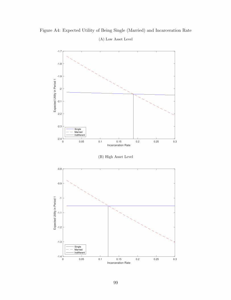
Figure A4: Expected Utility of Being Single (Married) and Incarceration Rate

(A) Low Asset Level

0 0.05 0.1 0.15 0.2 0.25 0.3

Incarceration Rate

-2.4

-2.3

-2.2

-2.1

-2

-1.9

-1.8

-1.7

Expecte

d U

tilit

y in P

eriod 1

Single

Married

Indifferent

(B) High Asset Level

0 0.05 0.1 0.15 0.2 0.25 0.3

Incarceration Rate

-1.4

-1.3

-1.2

-1.1

-1

-0.9

-0.8

Expecte

d U

tilit

y in P

eriod 1

Single

Married

Indifferent

99

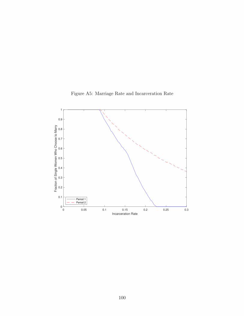
Figure A5: Marriage Rate and Incarceration Rate

0 0.05 0.1 0.15 0.2 0.25 0.3

Incarceration Rate

0

0.1

0.2

0.3

0.4

0.5

0.6

0.7

0.8

0.9

1

Fra

ction o

f S

ingle

Wom

en W

ho C

hoose to M

arr

y

Period 1

Period 2

100

Table A1: Availability of the NCRP Data

States Yearend Prison Population Admissions & Releases

Arkansas 2005-2009 1989-2009California 2004-2009 1983-2009Colorado 2009 1985-2009Florida 2004-2009 1995-2009Georgia∗ 2004-2009 1988-2009Louisiana 2004-2009 1992-2009Maryland∗∗ 2004-2009 1983-2009Michigan 2004-2006, 2008 1984-2009Minnesota 2004-2009 1998-2009Missouri 2004-2009 1998-2009New Jersey 2004-2005 1984-2009New York 2004-2009 1988-2009North Carolina 2004-2009 2004-2009Oklahoma 2004-2006, 2008 1986-2009Oregon 2004-2009 1984-2009Pennsylvania 2004-2009 1998-2009South Carolina 2004-2009 1987-2009Tennessee 2004-2009 1989-2009Texas 2004-2009 1985-2009Virginia 2009 1985-2009Washington 2004-2009 1985-2009Wisconsin 2004-2007 1983-2009

Note: The table only shows states that provide NCRP Yearend Prison PopulationData for at least one year. Column 2 shows the years during which Yearend PrisonPopulation Data were available. Column 2 shows the years during which Admis-sions and Releases Data were regularly submitted. (Records before 1986 were eithermissing or unreasonably small in most states. Records in some years in the middleof the time periods can be missing as well.)∗ Admissions and Releases Data for Georgia are not reliable because prison popula-tion backed out using the perpetual inventory method are mostly negative. There-fore, only data in 2004-2009 for Georgia will be included in the sample.∗∗ Maryland is excluded from the sample. According to the codebooks, the ana-lytical value of the data for Maryland is limited due to a continuing problem inmaintaining data entry accuracy.

101

Table A2: Impact of Black Male Incarceration on Black Women’s Education

Dependent variable Years of educationOLS 2SLS 2SLS(1) (2) (3)

Fraction of black -2.360* -5.788 -4.721men in prison (1.273) (5.544) (5.466)

Observations 327,456 327,456 327,456R-squared 0.036 0.036 0.082Mean of dep. var. 12.689SD of dep. var. 2.041Year & MSA FEs Yes Yes YesControl variables Yes

Note: The sample includes MSAs with at least 1,000 blackmen and 1,000 black women ages 20-34. The analysis isrestricted to black women ages 18-34. Control variablesinclude age and age-squared. Standard errors are clusteredat the MSA level. Robust standard errors in parentheses:*** p<0.01, ** p<0.05, * p<0.1.

Table A3: Impact of Black Male Incarceration on Black Women’s Fertility

Dependent variable Have a child or childrenSamples Black women with some college Black women with no college

OLS 2SLS 2SLS OLS 2SLS 2SLS(1) (2) (3) (4) (5) (6)

Fraction of black 0.714 0.612 0.815 0.372 0.790 1.320men in prison (0.532) (1.534) (1.198) (0.392) (1.112) (0.993)

Observations 119,511 119,511 116,668 166,300 166,300 166,300R-squared 0.031 0.031 0.260 0.026 0.026 0.212Mean of dep. var. 0.500 0.572SD of dep. var. 0.500 0.495Year & MSA FEs Yes Yes Yes Yes Yes YesControl variables Yes Yes

Note: The sample includes MSAs with at least 1,000 black men and 1,000 black women ages 20-34. Columns 1-3 include black women ages 18-34 with some college education (without degrees) andColumns 4-6 include black women ages 18-34 without any college education. Control variables includeage, age-squared, and years of education. Standard errors are clustered at the MSA level. Robuststandard errors in parentheses: *** p<0.01, ** p<0.05, * p<0.1.

102

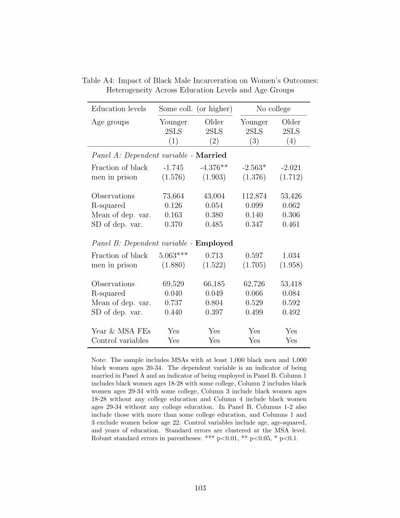
Table A4: Impact of Black Male Incarceration on Women’s Outcomes:Heterogeneity Across Education Levels and Age Groups

Education levels Some coll. (or higher) No college

Age groups Younger Older Younger Older2SLS 2SLS 2SLS 2SLS(1) (2) (3) (4)

Panel A: Dependent variable - Married

Fraction of black -1.745 -4.376** -2.563* -2.021men in prison (1.576) (1.903) (1.376) (1.712)

Observations 73,664 43,004 112,874 53,426R-squared 0.126 0.054 0.099 0.062Mean of dep. var. 0.163 0.380 0.140 0.306SD of dep. var. 0.370 0.485 0.347 0.461

Panel B: Dependent variable - Employed

Fraction of black 5.063*** 0.713 0.597 1.034men in prison (1.880) (1.522) (1.705) (1.958)

Observations 69,529 66,185 62,726 53,418R-squared 0.040 0.049 0.066 0.084Mean of dep. var. 0.737 0.804 0.529 0.592SD of dep. var. 0.440 0.397 0.499 0.492

Year & MSA FEs Yes Yes Yes YesControl variables Yes Yes Yes Yes

Note: The sample includes MSAs with at least 1,000 black men and 1,000black women ages 20-34. The dependent variable is an indicator of beingmarried in Panel A and an indicator of being employed in Panel B. Column 1includes black women ages 18-28 with some college, Column 2 includes blackwomen ages 29-34 with some college, Column 3 include black women ages18-28 without any college education and Column 4 include black womenages 29-34 without any college education. In Panel B, Columns 1-2 alsoinclude those with more than some college education, and Columns 1 and3 exclude women below age 22. Control variables include age, age-squared,and years of education. Standard errors are clustered at the MSA level.Robust standard errors in parentheses: *** p<0.01, ** p<0.05, * p<0.1.

103

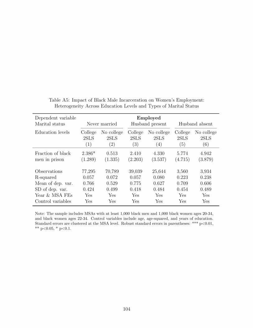
Table A5: Impact of Black Male Incarceration on Women’s Employment:Heterogeneity Across Education Levels and Types of Marital Status

Dependent variable EmployedMarital status Never married Husband present Husband absent

Education levels College No college College No college College No college2SLS 2SLS 2SLS 2SLS 2SLS 2SLS(1) (2) (3) (4) (5) (6)

Fraction of black 2.386* 0.513 2.410 4.330 5.774 4.942men in prison (1.289) (1.335) (2.203) (3.537) (4.715) (3.879)

Observations 77,295 70,789 39,039 25,644 3,560 3,934R-squared 0.057 0.072 0.057 0.080 0.223 0.238Mean of dep. var. 0.766 0.529 0.775 0.627 0.709 0.606SD of dep. var. 0.424 0.499 0.418 0.484 0.454 0.489Year & MSA FEs Yes Yes Yes Yes Yes YesControl variables Yes Yes Yes Yes Yes Yes

Note: The sample includes MSAs with at least 1,000 black men and 1,000 black women ages 20-34,and black women ages 22-34. Control variables include age, age-squared, and years of education.Standard errors are clustered at the MSA level. Robust standard errors in parentheses: *** p<0.01,** p<0.05, * p<0.1.

104

Table A6: Impact of Black Male Incarceration on Black Men’s Outcomes

Dependent variables Married White wife Employed2SLS 2SLS 2SLS(1) (2) (3)

Panel A: Impact on black men with some college

Fraction of black -1.568 1.726* 0.00438men in prison (1.418) (0.884) (1.141)

Observations 136,962 136,962 125,808R-squared 0.182 0.042 0.059Mean of dep. var. 0.318 0.0411 0.819SD of dep. var. 0.466 0.198 0.385

Panel B: Impact on black men with no college

Fraction of black -1.461 -0.214 -3.077*men in prison (1.196) (0.592) (1.633)

Observations 165,666 165,666 144,810R-squared 0.112 0.039 0.062Mean of dep. var. 0.273 0.0325 0.667SD of dep. var. 0.446 0.177 0.471

Year & MSA FEs Yes Yes YesControl variables Yes Yes Yes

Note: The sample includes MSAs with at least 1,000 black women and1,000 black men ages 20-34. Panel A includes black men ages 22-39with some college education, and Panel B includes black men ages22-29 without any college education. Control variables include age,age-squared, and years of education. Standard errors are clustered atthe MSA level Robust standard errors in parentheses: *** p<0.01, **p<0.05, * p<0.1.

105

Table A7: Robustness Test: Alternative Simulated Instrumental Variables

Dependent Live with Out-of-variables Married Employed mother wedlock

Some coll. No college College No college only birth2SLS 2SLS 2SLS 2SLS 2SLS 2SLS(1) (2) (3) (4) (5) (6)

Panel A: Baseline simulated IV

Fraction of black -3.121*** -2.640* 2.989** 0.821 3.533** 4.292**men in prison (0.964) (1.426) (1.180) (1.491) (1.767) (2.009)

F-statistics 27.136 23.768 17.471 23.408 28.096 19.964

Panel B: Simulated IV with drug-related offenses

Fraction of black -6.474*** -1.343 2.404** 2.584 2.847 2.036*men in prison (2.378) (0.964) (1.160) (1.754) (3.405) (1.078)

F-statistics 6.809 10.164 6.172 9.375 13.421 17.287

Note: In Columns 1-2, the dependent variable is an indicator of being married; the sample includes MSAswith at least 1,000 black men and 1,000 black women ages 20-34, and black women ages 18-34 with somecollege education (Column 1) and without any college education (Column 2). In Columns 3-4, the dependentvariable is an indicator of being employed; the sample includes MSAs with at least 1,000 black men and1,000 black women ages 20-34, and black women ages 22-34 with at least some college education (Column3) and without any college education (Column 4). In Column 5, the dependent variable is an indicator ofliving with mother only; the sample includes MSAs with at least 2000 black children age 0-14, and blackchildren age 0-14. In Column 6, the dependent variable is an indicator that mother is never married; thesample includes MSAs with at least 2000 newly born black infants, and black children below age 2. Controlvariables include age, age-squared, and years of education in Columns 1-4, age and sex in Column 5, andsex in Column 6. Standard errors are clustered at the state level. Robust standard errors in parentheses:*** p<0.01, ** p<0.05, * p<0.1

106

Table A8: Robustness Test: Alternative Measures of Black Male Incarceration

Dependent Live with Out-of-variables Married Employed mother wedlock

Some coll. No college College No college only birth2SLS 2SLS 2SLS 2SLS 2SLS 2SLS(1) (2) (3) (4) (5) (6)

Panel A: Independent variable - fraction of black men ages 20-54 in prison (baseline)

Fraction of black -3.121** -2.640** 2.989*** 0.821 3.533*** 4.292***men in prison (1.324) (1.156) (1.100) (1.306) (1.119) (1.495)

Mean of indep. var. 0.063 0.062 0.062 0.062 0.063 0.063F-statistics 42.697 43.003 34.823 42.657 46.728 47.32

Panel B: Independent variable - fraction of black men ages 20-39 in prison

Fraction of black -1.761** -1.535** 1.672*** 0.491 1.995*** 2.432***men in prison (0.786) (0.689) (0.643) (0.800) (0.632) (0.879)

Mean of indep. var. 0.102 0.099 0.101 0.099 0.102 0.102F-statistics 35.404 36.003 30.588 36.171 40.633 39.774

Panel C: Independent variable - fraction of single black men ages 20-54 in prison

Fraction of single -1.799** -1.503** 1.601** 0.494 2.280*** 2.391**black men in prison (0.850) (0.748) (0.680) (0.862) (0.658) (0.943)

Mean of indep. var. 0.090 0.089 0.089 0.089 0.090 0.090F-statistics 42.945 51.41 34.995 49.358 56.917 49.125

Panel D: Independent variable - sex ratio of single blacks ages 20-34 without college

Sex ratio 0.720* 0.999** -0.872** -0.441 -1.329** -0.682(0.413) (0.470) (0.427) (0.549) (0.602) (0.524)

Mean of indep. var. 0.801 0.793 0.806 0.790 0.800 0.800F-statistics 11.943 8.782 9.382 6.499 6.281 7.484

Note: In Columns 1-2, the dependent variable is an indicator of being married; the sample includes MSAs withat least 1,000 black men and 1,000 black women ages 20-34, and black women ages 18-34 with some collegeeducation (Column 1) and without any college education (Column 2). In Columns 3-4, the dependent variableis an indicator of being employed; the sample includes MSAs with at least 1,000 black men and 1,000 blackwomen ages 20-34, and black women ages 22-34 with at least some college education (Column 3) and withoutany college education (Column 4). In Column 5, the dependent variable is an indicator of living with motheronly; the sample includes MSAs with at least 2000 black children age 0-14, and black children age 0-14. InColumn 6, the dependent variable is an indicator that mother is never married; the sample includes MSAswith at least 2000 newly born black infants, and black children below age 2. Control variables include age,age-squared, and years of education in Columns 1-4, age and sex in Column 5, and sex in Column 6. Standarderrors are clustered at the MSA level. Robust standard errors in parentheses: *** p<0.01, ** p<0.05, * p<0.1

107

Table A9: Robustness Test: Concentration of Black Population within States

Dependent Live with Out-of-variables Married Employed mother wedlock

Some coll. No college College No college only birth2SLS 2SLS 2SLS 2SLS 2SLS 2SLS(1) (2) (3) (4) (5) (6)

Panel A: Baseline

Fraction of black -3.121** -2.640** 2.989*** 0.821 3.533*** 4.292***men in prison (1.324) (1.156) (1.100) (1.306) (1.119) (1.495)

Mean of indep. var. 0.063 0.062 0.062 0.062 0.063 0.063

Panel B: MSAs in states with HHI < 3500

Fraction of black -4.540* -5.437** 4.379** -1.557 6.796*** 6.613**men in prison (2.321) (2.320) (2.007) (2.224) (2.008) (2.610)

Mean of indep. var. 0.068 0.065 0.068 0.065 0.067 0.066

Note: In Panel A, the sample includes MSAs with at least 1,000 black men and 1,000 black women ages 20-34in Columns 1-4, MSAs with at least 2000 black children ages 0-14 in Column 5, and MSAs with at least 2000black children ages 0-4 in Column 6. In Panel B, the sample includes states where the HHI of black populationis smaller than 3500: including Arkansas, California, Florida, Louisiana, North Carolina, Oklahoman, SouthCarolina, Tennessee, Texas, and Virginia. Control variables include age, age-squared, and years of educationof black women (ages 20-34) in Columns 1-4, age and sex of black children (ages 0-14) in Column 5, and sexof black infants in Column 6. Standard errors are clustered at the MSA level. Robust standard errors inparentheses: *** p<0.01, ** p<0.05, * p<0.1.

108

Tab

leA

10:

Rob

ust

nes

sT

est:

Reg

ress

ions

wit

hL

aggi

ng

and

Lea

din

gIn

stru

men

ts

Dep

enden

tFra

ctio

nof

bla

ckL

ive

wit

hO

ut-

of-

vari

able

sm

en

inpri

son

Marr

ied

Em

plo

yed

moth

er

on

lyw

ed

lock

bir

th

(1)

(2)

(3)

(4)

(5)

(6)

(7)

(8)

(9)

(10)

IVt

0.02

79**

*0.

0094

4*-0

.074

7***

-0.1

68**

0.04

62*

-0.0

962

0.09

15**

*0.

255*

**0.

0872

**0.

0934

(0.0

0426

)(0

.004

88)

(0.0

278)

(0.0

658)

(0.0

262)

(0.0

949)

(0.0

256)

(0.0

759)

(0.0

419)

(0.1

19)

IVt−

1-0

.002

690.

0677

-0.0

0188

-0.0

510

-0.1

05(0

.004

56)

(0.0

766)

(0.1

17)

(0.0

781)

(0.1

74)

IVt−

20.

0077

0-0

.097

80.

0634

0.02

61-0

.130

(0.0

0523

)(0

.073

7)(0

.094

9)(0

.079

6)(0

.150

)IVt−

30.

0079

60.

0471

-0.0

383

0.00

0504

0.18

7*(0

.005

03)

(0.0

434)

(0.0

682)

(0.0

559)

(0.0

985)

IVt+

10.

0057

10.

0392

0.03

43-0

.039

60.

105

(0.0

0361

)(0

.070

0)(0

.100

)(0

.091

9)(0

.226

)IVt+

20.

0014

8-0

.000

770

0.00

836

-0.1

120.

153

(0.0

0277

)(0

.127

)(0

.078

9)(0

.078

1)(0

.156

)IVt+

30.

0026

1-0

.032

60.

109

0.02

45-0

.176

*(0

.003

82)

(0.0

782)

(0.0

882)

(0.0

697)

(0.1

07)

Obse

rvat

ions

327,

456

211,

630

166,

300

126,

430

209,

248

147,

248

661,

425

488,

710

123,

167

91,6

48R

-squar

ed0.

869

0.89

90.

107

0.10

40.

062

0.06

90.

022

0.02

70.

039

0.05

1L

eads=

00.

286

0.84

30.

142

0.24

60.

272

Not

e:T

he

sam

ple

incl

ud

esM

SA

sw

ith

atle

ast

1,0

00

bla

ckm

enan

d1,0

00

bla

ckw

om

enages

20-3

4in

Colu

mn

s1-6

,M

SA

sw

ith

at

least

200

bla

ckch

ild

ren

ages

0-14

inC

olu

mn

s7-

8,an

dM

SA

sw

ith

at

least

2000

bla

ckch

ild

ren

chil

dre

nages

0-4

inC

olu

mns

9-1

0.

An

aly

sis

isre

stri

cted

tob

lack

wom

enag

es18

-34

wit

hou

tany

coll

ege

edu

cati

on

inC

olu

mn

s1-4

,b

lack

wom

enages

22-3

4w

ith

at

least

som

eco

lleg

eed

uca

tion

inC

olu

mn

s5-

6,b

lack

chil

dre

nag

es0-1

4in

Colu

mn

s7-8

,an

db

lack

infa

nts

inC

olu

mn

s9-1

0.

MS

Aan

dyea

rfi

xed

effec

ts,

an

dco

ntr

ols

vari

able

sar

ein

clu

ded

.S

tan

dard

erro

rsare

clu

ster

edat

the

MS

Ale

vel.

Rob

ust

stan

dard

erro

rsin

pare

nth

eses

:***

p<

0.0

1,

**

p<

0.05

,*

p<

0.1.

109

Table A11: Robustness Test: Potential Confounds

Dependent Share of black Violent Propertyvariables population crime rate crime rate

(1) (2) (3)

Simulated IV -0.000211 0.00236 0.0195(0.00512) (0.0122) (0.0567)

Observations 327,456 327,456 327,456R-squared 0.992 0.818 0.883Mean of indep. var.

Note: The sample includes MSAs with at least 1,000 black men and 1,000 blackwomen ages 20-34, and analysis is restricted to black women ages 18-34. InColumn 1, the share of black population is measured at the MSA level. Yearand MSA fixed effects, and control variables for women are included. Standarderrors are clustered at the MSA level. In Columns 2-3, crime rates are measuredat the state level. Year and state fixed effects, and control variables for womenare included. Standard errors are clustered at the state level. Robust standarderrors in parentheses: *** p<0.01, ** p<0.05, * p<0.1.

110

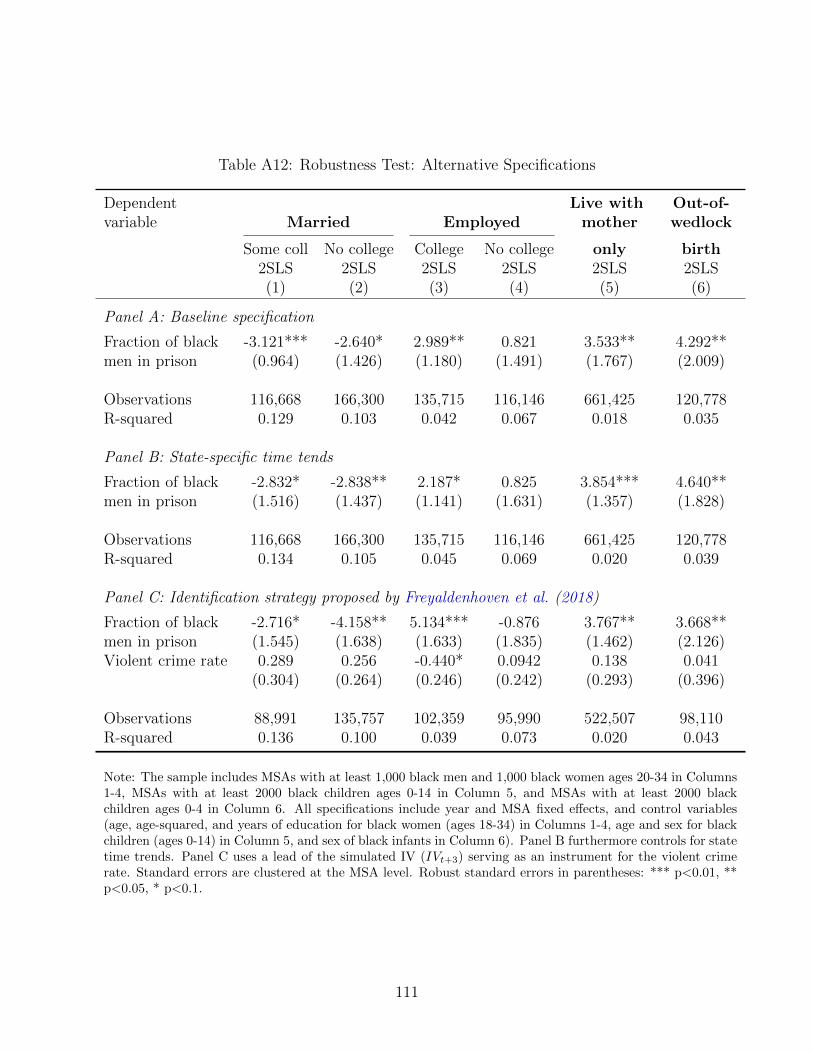
Table A12: Robustness Test: Alternative Specifications

Dependent Live with Out-of-variable Married Employed mother wedlock

Some coll No college College No college only birth2SLS 2SLS 2SLS 2SLS 2SLS 2SLS(1) (2) (3) (4) (5) (6)

Panel A: Baseline specification

Fraction of black -3.121*** -2.640* 2.989** 0.821 3.533** 4.292**men in prison (0.964) (1.426) (1.180) (1.491) (1.767) (2.009)

Observations 116,668 166,300 135,715 116,146 661,425 120,778R-squared 0.129 0.103 0.042 0.067 0.018 0.035

Panel B: State-specific time tends

Fraction of black -2.832* -2.838** 2.187* 0.825 3.854*** 4.640**men in prison (1.516) (1.437) (1.141) (1.631) (1.357) (1.828)

Observations 116,668 166,300 135,715 116,146 661,425 120,778R-squared 0.134 0.105 0.045 0.069 0.020 0.039

Panel C: Identification strategy proposed by Freyaldenhoven et al. (2018)

Fraction of black -2.716* -4.158** 5.134*** -0.876 3.767** 3.668**men in prison (1.545) (1.638) (1.633) (1.835) (1.462) (2.126)Violent crime rate 0.289 0.256 -0.440* 0.0942 0.138 0.041

(0.304) (0.264) (0.246) (0.242) (0.293) (0.396)

Observations 88,991 135,757 102,359 95,990 522,507 98,110R-squared 0.136 0.100 0.039 0.073 0.020 0.043

Note: The sample includes MSAs with at least 1,000 black men and 1,000 black women ages 20-34 in Columns1-4, MSAs with at least 2000 black children ages 0-14 in Column 5, and MSAs with at least 2000 blackchildren ages 0-4 in Column 6. All specifications include year and MSA fixed effects, and control variables(age, age-squared, and years of education for black women (ages 18-34) in Columns 1-4, age and sex for blackchildren (ages 0-14) in Column 5, and sex of black infants in Column 6). Panel B furthermore controls for statetime trends. Panel C uses a lead of the simulated IV (IVt+3) serving as an instrument for the violent crimerate. Standard errors are clustered at the MSA level. Robust standard errors in parentheses: *** p<0.01, **p<0.05, * p<0.1.

111

Table A13: Placebo Test: Impact of Black Male Incarceration onWhite Women and Children’s Outcomes

Dependent Live with Out-of-variable Married Employed mother wedlock

Some coll. No college College No college only birth2SLS 2SLS 2SLS 2SLS 2SLS 2SLS(1) (2) (3) (4) (5) (6)

Fraction of black 0.00405 -0.835 -0.387 0.509 -0.553 -0.133men in prison (0.819) (1.064) (0.652) (0.652) (0.802) (0.720)

Observations 701,748 811,761 1,025,145 577,222 3,766,166 715,064R-Squared 0.270 0.204 0.024 0.056 0.009 0.019Mean of dep. var. 0.391 0.470 0.781 0.586 0.160 0.125Std dev of dep. var. 0.488 0.499 0.414 0.493 0.367 0.330Year & MSA FEs Yes Yes Yes Yes Yes YesControl variables Yes Yes Yes Yes Yes Yes

Note: Analysis is restricted to white women ages 18-34 in Columns 1-2, white women ages 22-34 in Columns3-4, white children ages 0-14 in Column 5, and white infants in Column 6. Control variables include age,age-squared, and years of education in Columns 1-4, age and sex in column 5, and sex in Column 6. Standarderrors are clustered at the MSA level. Robust standard errors in parentheses: *** p<0.01, ** p<0.05, * p<0.1.

112

Table A14: Robustness Check: Black Population

Dependent Live with Out-of-variable Married Employed mother wedlock

Some coll. No college College No college only birth2SLS 2SLS 2SLS 2SLS 2SLS 2SLS(1) (2) (3) (4) (5) (6)

Panel A: Baseline: MSAs with black population (ages 20-34) > 2000

Fraction of black -3.121** -2.640** 2.989*** 0.821 3.533*** 4.292***men in prison (1.324) (1.156) (1.100) (1.306) (1.119) (1.495)

Mean of indep. var. 0.063 0.062 0.062 0.062 0.063 0.063

Panel B: All MSAs

Fraction of black -5.420*** -2.046* 2.956* 1.401 4.295*** 4.151*men in prison (1.504) (1.126) (1.515) (1.433) (1.375) (2.155)

Mean of indep. var. 0.063 0.062 0.062 0.062 0.063 0.063

Panel C: MSAs with fraction of black men in prison < 20%

Fraction of black -5.221*** -2.041* 2.545* 1.395 4.235*** 3.965*men in prison (1.430) (1.122) (1.328) (1.428) (1.348) (2.075)

Mean of indep. var. 0.063 0.062 0.062 0.062 0.063 0.063

Note: In Panel A, the sample includes MSAs with at least 1,000 black men and 1,000 black women ages 20-34in Columns 1-4, MSAs with at least 2000 black children ages 0-14 in Column 5, and MSAs with at least 2000black children ages 0-4 in Column 6. In Panel B, the sample includes all MSAs. In Panel C, the sampleincludes MSAs where the incarceration rates of black men is smaller than 20%. Analysis is restricted to blackwomen ages 19-34 with some college education or no college education in Columns 1-2, black women ages22-34 with at least some college education or no college eduction in Columns 3-4, black children ages 0-14 inColumn 5, black infants in Column 6. Control variables include age, age-squared, and years of education inColumns 1-4, age and sex in Column 5, and sex in Column 6. Standard errors are clustered at the MSA level.Robust standard errors in parentheses: *** p<0.01, ** p<0.05, * p<0.1.

113