in the name of the father: marriage and intergenerational ... 1. summary statistics for...

In the Name of the Father: Marriage andIntergenerational Mobility in the United States,

1850-1930.

Claudia Olivetti and M. Daniele Paserman

BU and NBER

November 2012

Olivetti and Paserman (BU and NBER) Marriage and Intergenerational Mobility November 2012 1 / 53

Introduction

Why intergenerational mobility?

Key for understanding the importance of family background indetermining economic outcomes.In the US, tolerance for high inequality sometimes explained by thebelief that mobility is also high (Alesina et al., 2004)American exceptionalism?

In fact, mobility in the US is among the lowest in OECD (Corak,2011).

Has it always been this way?


Introduction

Ferrie (2005) and Long and Ferrie (2007, forthcoming) establish thatmobility in the US was higher in the 19th Century.

Typically, people look at the relationship between father’s and son’seconomic standing.

This misses part of the picture: daughters.

How is the average status of one generation (both sons and daughters)related to that of their parents?Daughters can have an important role in transmitting status over tothe next generation. Mobility over three generations?


Intergenerational Mobility Literature

Vast literature based on modern linked longitudinal data sets (Solon,1999, Black and Devereux, 2010):

Mostly focused on father/son correlations.Few studies on father/son-in-law correlation: evidence that it is smallerthan father/son correlation.

Historical literature based on data obtained linking individuals by firstand last name across Census decades (Ferrie, 2005).

Can construct father/son links and estimate father/son correlations.But impossible to construct father/daughter links because daughterschange last name upon marriage.


Our Contribution

Develop methodology that allows estimation of intergenerationalelasticities even without individually linked data.

Construct synthetic cohorts using information on first namesCan be applied equally to sons and daughters

Investigate gender differentials in intergenerational mobility during1850-1930 period by calculating elasticities in occupational income:

Father/sonFather/son-in-law


Basic Idea

First names contain information about economic status.

Suppose that in generation t high SES adults call their sons Adam,low SES call their sons Zachary.

What happens in generation t + 1? Are the Adam still higher SESthan the Zacharys?

If yes, we would say that there is relatively little mobility. If no, highmobility.

Nice feature of this methodology: can be applied just as easily toAbigails and Zoes.


Preview of the Findings

Intergenerational elasticity between fathers and sons (ηSON) shows a30% increase between 1870 and 1930.

Consistent with ”the end of American exceptionalism” (Ferrie, 2005,Long and Ferrie, 2007, forthcoming).

Intergenerational elasticity between fathers and sons-in-law (ηSIL):

Trend similar to that of ηSON , although timing of the increase slightlydifferent.By the end of the sample period is lower than ηSON in mostspecifications – similar to results for modern studies.

Results likely driven by changes in the parameters of the incometransmission process, not changes in the distribution of names.

Results robust to different imputations of occupational income, namecoding and treatment of: farmers, immigrants, child mortality.


Outline

Introduction

Illustrative Model

Econometric Methodology

Data

Results

BenchmarkSimulations

Discussion


An Illustrative Model of Marriage and Mobility

Families containing 2 parents and 2 children: one male, one female.

Only men work.

Altruistic parents with consensus utility choose how to optimallyallocate lifetime earnings, yt−1, between own consumption andinvestment in children’s human capital.

Parents investment in children’s human capital determines:

Son’s earnings on the labor market, ytDaughter’s spouse earnings through the marriage market, ySIL,t

Optimal human capital investment proportional to yt−1.


Fathers and Sons

Reduced form earnings equation:

log yt = γ1 log yt−1 + et + ut

et = λet−1 + vt

γ1 = rate of return to human capital, γ1 ∈ (0, 1)et = child’s “endowment”, 0 ≤ λ < 1, vt i.i.d. with variance σ2

v .ut = “labor market luck” i.i.d. with variance σ2

u .

Father/son intergenerational elasticity, estimated by OLS:

ηSON ≡ p limCov(yt , yt−1)

Var(yt−1)= γ1 +

λ(1− γ2

1

)(1 + γ1λ) + (1− γ1λ) (σ2

u/σ2e )


Fathers and Sons-in-law

Reduced form earnings equations:

log ySIL,t = α1 log yt−1 + θet + µt

α1 = rate of return to female human capital in marriage marketµt = luck in the marriage market, i.i.d. with variance σ2

µ .θ : relative importance of family endowment for daughters.

Father/son-in-law intergenerational elasticity :

ηSIL ≡ p limCov(ySIL,t , yt−1)

Var(yt−1)

= α1 + θ

(λ(1− γ2

1

)(1 + γ1λ) + (1− γ1λ) (σ2

u/σ2e )

)


Econometric Methodology

With individually linked data:

Both yit and yit−1 observedIntergenerational elasticity obtained by regressing yit on yit−1Linked estimator: ηLINKED

In our data it is impossible to link individuals across cross-sections tand t − 1 but information on first names is available.


Econometric Methodology: Pseudo panel

Define:

yj ,t−1 = average log earnings of fathers of children named jin Census year t − 1yjt = average log earnings (as adults) of children named jin Census year t

Pseudo-panel estimator, ηPSEUDO , obtained by:

Merging two cross sections by first namesRegressing yjt on yjt−1 (weighted by name frequency)



Estimator is equivalent to Two Sample IV (2SIV or 2S2SLS)

First stage: Regress father’s income on matrix of sons’ first namedummies (sample 1)Second stage: Regress son’s income on fitted values from first stage(sample 2)

Alternative interpretation: father’s income is “generated regressor”

Actual father’s income replaced by predicted income by son’s firstname.



Key requirement:Names carry information about socioeconomic status.

If not:

Zero first stage“Generated regressor” is just noise.


Data

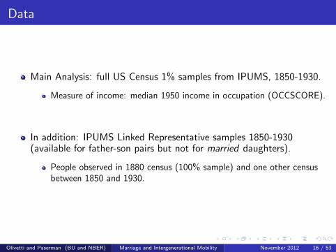
Main Analysis: full US Census 1% samples from IPUMS, 1850-1930.

Measure of income: median 1950 income in occupation (OCCSCORE).

In addition: IPUMS Linked Representative samples 1850-1930(available for father-son pairs but not for married daughters).

People observed in 1880 census (100% sample) and one other censusbetween 1850 and 1930.


Summary Statistics

(1) (2) (3) (4) (5) (6) (7) (8)

Year1850 35,597 3,524 10.1 71.9 7.1 92.6 0.6919 0.13431860 48,114 4,083 11.8 70.5 6.0 93.7 0.6946 0.11081870 58,039 4,582 12.7 69.4 5.5 0.6978 0.10531880 75,004 6,589 11.4 69.4 6.1 92.9 0.6529 0.11191900 103,817 9,696 10.7 71.0 6.6 92.8 0.5638 0.12651910 117,612 9,818 12.0 69.5 5.8 94.1 0.5342 0.1256

1850 34,272 3,442 10.0 71.9 7.2 92.4 0.6984 0.13571860 46,874 4,488 10.4 70.7 6.8 92.8 0.6573 0.13201870 55,739 5,206 10.7 71.1 6.6 0.6193 0.13561880 72,160 7,161 10.1 69.0 6.8 92.0 0.5475 0.13311900 101,516 10,081 10.1 70.9 7.0 92.3 0.4744 0.15261910 114,074 10,103 11.3 69.3 6.1 93.5 0.4726 0.1545

Males

Females

Table 1. Summary Statistics for Children's Names: 1850-1910

Number of children

ages 0-15

Number of distinct names

Mean number of observations

per name

Percent of names that

are singletons

Percent of children with unique names

Percent of children with

names linked 20 years later

Share with top-50 name

Share of total variation in log

earnings explained by between name

variation


Ranking of Names

1850 1860 1870 1880 1900 1910 1920 1930

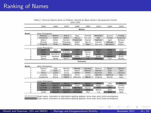
Rank:1 Edward Walter Harry Paul Donald Abraham Jerome Irving2 Frederick Frank Walter Harry Kenneth Max Irving Frederick3 Edwin Willie Herbert Frederick Harold Nathan Jack Richard4 Charles Louis Theodore Ralph Morris Vincent Nathan Roger5 Franklin Fred Edward Philip Max Edmund Abraham Robert

1 Jesse Levi Jesse Luther Luther Jessie Willie Jose2 Hiram Isaac Franklin Ira Dewey Otis Loyd Loyd3 Isaac Benjamin Isaac Isaac Perry Luther Luther Willie4 Daniel Andrew Hiram Willis Virgil Eddie Jessie Ervin5 David Jacob Martin Charley Ira Charley Otis Archie

Rank:1 Emma Ada Bertha Bessie Dorothy Eleanor Betty Jeanne2 Alice Kate Jessie Mabel Marion Marian Jean Jane3 Anna Lizzie Grace Helen Helen Dorothy Jane Carolyn4 Isabella Clara Carrie Ethel Louise Marion Kathryn Ann5 Josephine Fanny Helen Blanche Marie Virginia Muriel Joan

1 Sally Amanda Nancy Nancy Nancy Sallie Lela Eula2 Nancy Nancy Lucinda Viola Ollie Addie Maggie Lorene3 Lucinda Rachel Rebecca Martha Nannie Ollie Ollie Dortha4 Martha Lucinda Amanda Rachel Sallie Mattie Effie Willie5 Lydia Martha Martha Amanda Alta Iva Eula Opal

Exact name, nickname or alternative spelling appears more than once (most prestigious).Exact name, nickname or alternative spelling appears more than once (least prestigious).

Most Prestigious

Least Prestigious

Most Prestigious

Least Prestigious

Table 2: Common Names Given to Children, Ranked by Mean Father's Occupational Income 1850-1930.

Females

Males


Benchmark Results

Figure 1: Father/Son and Father/Son in Law Elasticities inOccupational Income

.3.3

5.4

.45

.5

1860 1870 1880 1890 1900 1910 1920 1930Year

Father/Son Father/Son-in-Law


Benchmark Results

(1) (2) (3) (4) (5)

1850-1870 1860-1880 1880-1900 1900-1920 1910-1930Sample:Sons: baseline 0.3500 0.3133 0.3440 0.4953 0.4760

(0.0239) (0.0200) (0.0166) (0.0152) (0.0118)[37077, 1182] [50847, 1478] [80255, 2234] [109079, 3253] [122468, 3720]

Son's Age 5-15 0.3286 0.3050 0.3574 0.4527 0.4199(0.0293) (0.0243) (0.0203) (0.0173) (0.0134)

[24336, 984] [32657, 1257] [53629, 1860] [76365, 2782] [83920, 3257]

Married Sons 0.2868 0.3433 0.3805 0.4715 0.4428(0.0312) (0.0260) (0.0223) (0.0178) (0.0133)

[17912, 891] [24510, 1155] [36521, 1641] [57570, 2586] [67137, 3051]

Sons in law: baseline 0.3402 0.4009 0.3992 0.4932 0.4136(0.0213) (0.0191) (0.0183) (0.0131) (0.0100)[23280, 976] [30081, 1376] [45804, 2063] [68439, 2888] [79314, 3326]

Daughter's Age 5-15 0.3440 0.3991 0.3918 0.5013 0.4186(0.0256) (0.0232) (0.0214) (0.0152) (0.0116)

[17019, 839] [22037, 1203] [34712, 1825] [52967, 2565] [61308, 2979]

Sons in law 20-35 0.3283 0.4394 0.3860 0.4889 0.4143(0.0250) (0.0224) (0.0218) (0.0151) (0.0116)

[15404, 840] [20383, 1197] [30533, 1712] [46762, 2479] [54600, 2885]

Sons: Individually linked data 0.4654 0.4751(0.0175) (0.0120)

3947 8847

Table 3. Intergenerational Elasticities in Occupational Income, 1850-1930.


Basic findings

Father/son intergenerational elasticity increases over time.

Father/son-in-law elasticity also increases, but timing is slightlydifferent.

Increase happens earlier, but ηSIL lower than ηSON at the end of theperiod.Results almost identical when we make sons and sons-in-law samplescomparable.

Pseudo-panel estimator lower than individually-linked estimator byabout 28-33%.


Robustness Checks

Results are robust to:

Imputation of farmer’s income (use 1901 wage distribution, excludefarmers, etc.).

Alternative measures of log occupational income (income rank, 1990distribution, SEI).

Controls for age (both fathers and sons).


Can trends be explained by changing name distribution?

ηSON goes from 0.31 to 0.48 between 1860-1880 and 1910-1930.

Can this be driven by changes in name distribution?

Numerical exercise:

Simulate income and name generating process

Set model parameters to match simulated moments to their datacounterparts for 1860-1880.

How does the estimate of ηSON change as we vary the parametersgoverning:

1 The name distribution?2 The income process?


Numerical Simulations

Income generating process:

log yt = γ1 log yt−1 + et + ut

et = λet−1 + vtut ∼ N

(0, σ2

u

); vt ∼ N

(0, σ2

v

)Name assignment process:

P (Name = j) =exp (δCON,j + δSES,jet−1)

∑j exp (δCON,j + δSES ,jet−1).

δCON,j ∼ N(0, σ2

CON

); δSES,j ∼ N

(0, σ2

SES

).

σ2CON = concentration of names: high σ2

CON , high concentration.

σ2SES = sensitivity of names to SES


Numerical Simulations

Generate population of N = 500, 000 families, J = 1, 500 names.

Generate income and assign names.

Create:

10% individually linked father/son sample10% father-son pseudo-panel linked by first namesN and J chosen so that extracts match 1860 Census data.

Estimate ψ =(γ1, λ, σ2

u , σ2v , σ2

CON , σ2SES

)by SMM.


Moments and Parameters

Moments Source

Cov(y t ,y t-1 )/V (y t-1 ) 1860-1880 Linked sampleV (y t-1 ) 1860-1880 Linked sampleCov PS (y t ,y t-1 )/V PS (y t-1 ) 1860 and 1880 1% samplesV PS (y t-1 ) 1860 1% sampleShare of top 50 names 1860 1% sampleR-squared 1860 1% sample

γ σ 2 u σ² v σ 2 CON σ 2 SES0.421 0.191 0.092 0.031 7.833 5.958

0.105 0.111

Distance minimizing parameters

0.314 0.3130.011 0.0110.695 0.695

0.158 0.160

Table 7. Moments and Parameters Used in the Simulations

Simulation Data

0.464 0.465


Sensitivity to the name distribution

(1) (2) (3) (4) (5) (6) (7)

Concetration of the name

distribution (2con)

0 1 3 5.958 10 20 30

2.5 η=0.0345 0.1131 0.2301 0.3107 0.3735 0.4343 0.4662

[share50= 0.3444] [0.344] [0.3437] [0.3452] [0.3468] [0.3542] [0.3651]

(R2=0.1078) (0.1139) (0.1269) (0.1421) (0.1592) (0.1897) (0.209)

5 0.0275 0.1073 0.2203 0.3087 0.3757 0.4385 0.4616

[0.5526] [0.5524] [0.5521] [0.5517] [0.552] [0.5542] [0.5584]

(0.0894) (0.0967) (0.1084) (0.1232) (0.1406) (0.1718) (0.1901)

7.833 0.0139 0.1160 0.2246 0.3144 0.3794 0.4494 0.4746

[0.6976] [0.6965] [0.6958] [0.6952] [0.6949] [0.6947] [0.6972](0.0713) (0.0774) (0.0898) (0.1053) (0.1215) (0.1519) (0.1716)

10 0.0146 0.1169 0.2324 0.3148 0.3890 0.457 0.48

[0.7638] [0.7638] [0.7636] [0.7623] [0.7615] [0.7609] [0.761]

(0.0605) (0.0666) (0.0774) (0.0922) (0.1098) (0.138) (0.1596)

15 0.0122 0.1209 0.2419 0.3385 0.4009 0.4703 0.4892[0.8444] [0.8447] [0.8438] [0.8428] [0.842] [0.8408] [0.8396]

(0.0441) (0.0498) (0.0599) (0.0736) (0.09) (0.1191) (0.1394)

Table 8. The Effects of the Features of the Name Distribution on Estimated Elasticities Simulation Results.

Socio-economic content of names (2ses)


Can trends be explained by changing name distribution?

To explain observed increase in ηSON we need massive increase inσ2SES , approximately from 2 to 20.

This implies that R2 in regression of father’s income on son’s namefixed effects also increases dramatically, from 0.12 to 0.20.

In practice, R2 constant around 0.12 over the period (Table 1)


Can this be driven by changes in the income process?

(1) (2) (4) (5) (6) (7)

Persistence of income ():

0 0.1 0.191 0.3 0.4 0.5

0.1 η=0.0502 0.1070 0.1543 0.2239 0.2931 0.3763

[share50=0.6953] [0.6952] [0.6952] [0.695] [0.6956] [0.6948]

(R2=0.105) (0.1057) (0.1081) (0.1109) (0.1168) (0.1268)

0.2 0.1024 0.1591 0.2080 0.2796 0.3496 0.4340[0.6953] [0.6952] [0.6952] [0.695] [0.6956] [0.6948]

(0.1039) (0.1053) (0.1081) (0.1115) (0.1182) (0.1292)

0.3 0.1518 0.2084 0.2591 0.3330 0.4039 0.4897

[0.6953] [0.6952] [0.6952] [0.695] [0.6956] [0.6948](0.1022) (0.1041) (0.1074) (0.1113) (0.1186) (0.1305)

0.421 0.2049 0.2613 0.3144 0.3915 0.4641 0.5522

[0.6953] [0.6952] [0.6952] [0.695] [0.6956] [0.6948]

(0.0992) (0.1016) (0.1053) (0.1097) (0.1175) (0.1303)

0.5 0.2331 0.2892 0.3438 0.4233 0.4975 0.5878

[0.6953] [0.6952] [0.6952] [0.695] [0.6956] [0.6948]

(0.0967) (0.0993) (0.1031) (0.1077) (0.1156) (0.1289)

0.6 0.2582 0.3137 0.3701 0.4526 0.5291 0.6236

[0.6953] [0.6952] [0.6952] [0.695] [0.6956] [0.6948]

(0.0928) (0.0956) (0.0994) (0.104) (0.1118) (0.1251)

Table 9. The Effects of Changes in the Income Generating Process on Intergenerational Pseudo-Elasticities Simulation Results.

Persistence of income shock ():

Much more likely that this is driven by real changes in the parametersgoverning the income process, γ1 and λ.


What factors can explain the trends?

Period under examination characterized by major economic anddemographic changes.

Dramatic drop in fertility and family size.

Migration – international and internal.

Regional differences in industrialization and economic development.

Investments in public education.


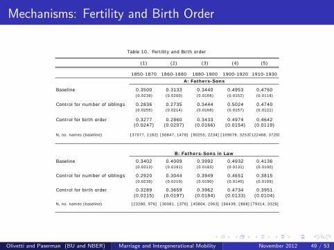
Fertility?

Increase in elasticity possible if fertility decline occurs earlier for highincome group.

High income parents can divide same wealth among fewer children.

Jones and Tertilt (2008): smooth fertilty transition for high-incomegroups, more abrupt for low-income groups.

But the timing is off: increase in elasticity should have occurred atthe end of the 19th Century.

Directly controlling for number of siblings and fort birth order has noeffect on the results (Table 10).


International Migration?

Common belief that migration can serve as one of the main enginesof social mobility.

Age of mass migration: 1880-1920.

But this implies that mobility should have increased during thisperiod, contrary to what we observe

Directly controlling for immigrant status (of both fathers and sons),has almost no effect on the coefficients (Table 11)


Internal Migration?

Long and Ferrie (2012) argue that internal migration is responsible forhigh intergenerational mobility: a form of investment in children’shuman capital.

Timing is more plausible: internal migration peaked in the middle ofthe 19th Century, then flat.

But directly controlling for internal mobility has no effect on theestimates (Table 11).

Caveat: we may not be able to control properly for internal mobility, nomeasure of within-state mobility.


Regional Differences?

Period of increase in intergenerational elasticity coincides with periodof economic divergence between regions.

Northeast and Midwest complete industrial transition, South stillagricultural and lags behind.

If relatively low mobility across regions, regional differences ineconomic development could explain the decline in mobility.

Controls for region fixed effects or state-level measures ofdevelopment: upward trend in elasticity all but disappears (Table 12).


Regional Differences?

(1) (2) (3) (4) (5)

1850-1870 1860-1880 1880-1900 1900-1920 1910-1930

All 0.3500 0.3133 0.3440 0.4953 0.4760(0.0239) (0.0200) (0.0166) (0.0152) (0.0118)

Control for state of residence 0.2765 0.1943 0.2108 0.2746 0.2799(0.0228) (0.0189) (0.0156) (0.0142) (0.0111)

Control for indicators of economic develop 0.2784 0.1975 0.2013 0.2633 0.2656(0.0228) (0.0188) (0.0156) (0.0142) (0.0110)

N, no. names (all) [37077, 1182] [50847, 1478] [80255, 2234] [109079, 3253][122468, 3720]

All 0.3402 0.4009 0.3992 0.4932 0.4136(0.0213) (0.0191) (0.0183) (0.0131) (0.0100)

Control of region of residence 0.2474 0.2947 0.2509 0.3199 0.2600(0.0205) (0.0182) (0.0175) (0.0127) (0.0099)

Control for indicators of economic develop 0.2513 0.2988 0.2517 0.3177 0.2550(0.0204) (0.0181) (0.0174) (0.0127) (0.0098)

N, no. names (all) [23280, 976] [30081, 1376] [45804, 2063] [68439, 2888] [79314, 3326]

Table 12. Intergenerational Elasticities 1850-1930. By Region of Birth.

A: Fathers-Sons

B: Fathers-Sons in Law


Public Schooling?

Increased investment in public schooling should increase mobility.

Timing is inconsistent with observed trends.

But analysis within regions does show that mobility was higher inregions with higher scholarization rates (Northeast and Midwest) thanin the South. (Table 13).


Increase in returns to human capital

Trends in ηSON consistent with improvements in men’s labor marketoutcomes that increase γ1:

Rise in returns to education (Goldin, 1999; Margo, 2000)Improved men’s career prospects (Cverk, 2011)

Trends in ηSIL:

With positive assortative mating, increases in γ1 also lead to increasesin the return to human capital in the marriage market.Also, imbalanced sex ratios induced by war and immigration couldaffect the returns to female human capital.


Conclusion

Propose a new method for estimating intergenerational elasticities inthe US in the late 19th-early 20th Century.

Applicable to both sons and daughters.

Large increases in both father/son and father/son-in-law elasticity.

Our preferred explanation: regional differences in economicdevelopment.


Thank you!


Robustness: Sensitivity to Farmer’s Income Imputations

(1) (2) (3) (4) (5)

1850-1870 1860-1880 1880-1900 1900-1920 1910-1930

Log occupational income in:

1950 0.3500 0.3133 0.3440 0.4953 0.4760(0.0239) (0.0200) (0.0166) (0.0152) (0.0118)

1900 0.3502 0.3542 0.3823 0.4471 0.4436(0.0222) (0.0189) (0.0155) (0.0121) (0.0101)

1900, imputed farmer wage 0.3467 0.2879 0.3634 0.4660 0.4701(0.0284) (0.0229) (0.0196) (0.0150) (0.0127)

1950 ex. farmers 0.1899 0.1561 0.1463 0.2540 0.2922(0.0476) (0.0359) (0.0280) (0.0322) (0.0277)

1900 ex. farmers 0.2487 0.2075 0.2320 0.2992 0.2954(0.0460) (0.0374) (0.0329) (0.0312) (0.0259)

1950 ex. farmers 0.2860 0.3266 (linked sample) (0.0495) (0.0340)

N, no. of names: 1950 [37077, 1182][50847, 1478][80255, 2234]109079, 3253[122468, 3720]

N, no. of names: 1950 ex. Farmers [26988, 741] [36460, 943][65726, 1529][92664, 2337][109830, 2845]

Table 4. Intergenerational Elasticities 1850-1930. Sensitivity to Farmers' Income Imputations.

A: Fathers-Sons


Robustness: Sensitivity to Farmer’s Income Imputations

1950 0.3402 0.4009 0.3992 0.4932 0.4136(0.0213) (0.0191) (0.0183) (0.0131) (0.0100)

1900 0.3115 0.4229 0.4120 0.4900 0.4387(0.0203) (0.0192) (0.0182) (0.0126) (0.0100)

1900, imputed farmer wage 0.2509 0.3161 0.3166 0.4415 0.4221(0.0242) (0.0205) (0.0208) (0.0146) (0.0120)

1950 ex. Farmers 0.2150 0.2003 0.1802 0.3270 0.3220(0.0465) (0.0303) (0.0284) (0.0288) (0.0227)

1900 ex. Farmers 0.1986 0.2290 0.2224 0.3490 0.3744(0.0403) (0.0316) (0.0297) (0.0289) (0.0248)

N, no. of names: 1950 [23280, 976] [30081, 1376][45804, 2063][68439, 2888][79314, 3326]N, no. of names: 1950 ex. Farmers [22586, 697] [29344, 1004][44917, 1547][67488, 2313][78026, 2724]



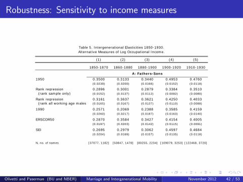
Robustness: Sensitivity to income measures

(1) (2) (3) (4) (5)

1850-1870 1860-1880 1880-1900 1900-1920 1910-1930

1950 0.3500 0.3133 0.3440 0.4953 0.4760(0.0239) (0.0200) (0.0166) (0.0152) (0.0118)

Rank regression 0.2896 0.3001 0.2879 0.3384 0.3510 (rank sample only) (0.0152) (0.0137) (0.0112) (0.0092) (0.0080)

Rank regression 0.3161 0.3637 0.3621 0.4250 0.4033 (rank all working age males) (0.0165) (0.0167) (0.0137) (0.0110) (0.0088)

1990 0.2571 0.2069 0.2388 0.3585 0.4159(0.0260) (0.0217) (0.0187) (0.0163) (0.0140)

ERSCOR50 0.2870 0.3584 0.3427 0.4154 0.4005(0.0197) (0.0203) (0.0142) (0.0115) (0.0091)

SEI 0.2695 0.2979 0.3062 0.4597 0.4684(0.0204) (0.0189) (0.0157) (0.0135) (0.0118)

N, no. of names [37077, 1182] [50847, 1478] [80255, 2234] [109079, 3253] [122468, 3720]

Table 5. Intergenerational Elasticities 1850-1930. Alternative Measures of Log Occupational Income.

A: Fathers-Sons


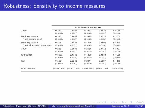
Robustness: Sensitivity to income measures

1950 0.3402 0.4009 0.3992 0.4932 0.4136(0.0213) (0.0191) (0.0183) (0.0131) (0.0100)

Rank regression 0.3301 0.4405 0.3975 0.4275 0.3700 (rank sample only) (0.0163) (0.0165) (0.0143) (0.0102) (0.0085)

Rank regression 0.3087 0.4429 0.4266 0.4902 0.4074 (rank all working age males) (0.0157) (0.0171) (0.0160) (0.0118) (0.0092)

1990 0.2137 0.2685 0.2586 0.4418 0.3997(0.0229) (0.0211) (0.0218) (0.0161) (0.0128)

ERSCOR50 0.3031 0.4746 0.4228 0.4934 0.4105(0.0196) (0.0218) (0.0175) (0.0123) (0.0096)

SEI 0.1887 0.3243 0.3244 0.5097 0.4879(0.0200) (0.0203) (0.0213) (0.0147) (0.0124)

N, no. of names [23280, 976] [30081, 1376] [45804, 2063] [68439, 2888] [79314, 3326]



Robustness: Controls for Age

(1) (2) (3) (4) (5) (6) (7) (8) (9) (10)

Variable:Father's Income 0.3500 0.3523 0.3133 0.3307 0.3440 0.3466 0.4953 0.4855 0.4760 0.4605

(0.0239) (0.0240) (0.0200) (0.0199) (0.0166) (0.0164) (0.0152) (0.0151) (0.0118) (0.0117)

Father's age 0.0096 0.0009 0.0289 0.0196 0.0183(0.0093) (0.0080) (0.0060) (0.0055) (0.0043)

Father's age squared -0.0001 -0.0001 -0.0004 -0.0002 -0.0002(0.0001) (0.0001) (0.0001) (0.0001) (0.0001)

Son's age 0.1075 0.0879 0.1014 0.0907 0.1174(0.0069) (0.0058) (0.0048) (0.0044) (0.0039)

Son's age squared -0.0017 -0.0013 -0.0015 -0.0014 -0.0018(0.0001) (0.0001) (0.0001) (0.0001) (0.0001)

N, no. of names

A: Fathers-Sons

Table 6. Intergenerational Elasticities 1850-1930. Age Controls.

1850-1870 1860-1880 1880-1900 1900-1920 1910-1930

[37077, 1182] [50847, 1478] [80255, 2234] [109079, 3253] [122468, 3720]


Robustness: Controls for Age

Father's Income 0.3402 0.3330 0.4009 0.3873 0.3992 0.3987 0.4932 0.4869 0.4136 0.4077(0.0213) (0.0219) (0.0191) (0.0192) (0.0183) (0.0183) (0.0131) (0.0134) (0.0100) (0.0102)

Father's age 0.0062 0.0106 0.0016 0.0093 0.0046(0.0100) (0.0085) (0.0073) (0.0059) (0.0040)

Father's age squared -0.0001 -0.0002 -0.0000 -0.0001 -0.0001(0.0001) (0.0001) (0.0001) (0.0001) (0.0000)

Son's age 0.0447 0.0328 0.0282 0.0179 0.0249(0.0029) (0.0020) (0.0018) (0.0013) (0.0013)

Son's age squared -0.0006 -0.0004 -0.0004 -0.0002 -0.0003(0.0000) (0.0000) (0.0000) (0.0000) (0.0000)

N, no. of names [23280, 976] [30081, 1376] [45804, 2063] [68439, 2888] [79314, 3326]



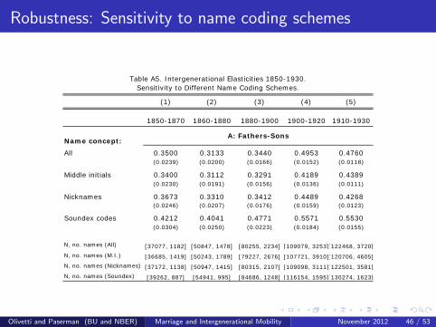
Robustness: Sensitivity to name coding schemes

(1) (2) (3) (4) (5)

1850-1870 1860-1880 1880-1900 1900-1920 1910-1930

Name concept:

All 0.3500 0.3133 0.3440 0.4953 0.4760(0.0239) (0.0200) (0.0166) (0.0152) (0.0118)

Middle initials 0.3400 0.3112 0.3291 0.4189 0.4389(0.0230) (0.0191) (0.0156) (0.0136) (0.0111)

Nicknames 0.3673 0.3310 0.3412 0.4489 0.4268(0.0246) (0.0207) (0.0176) (0.0159) (0.0123)

Soundex codes 0.4212 0.4041 0.4771 0.5571 0.5530(0.0304) (0.0250) (0.0223) (0.0184) (0.0155)

N, no. names (All) [37077, 1182] [50847, 1478] [80255, 2234] [109079, 3253][122468, 3720]N, no. names (M.I.) [36685, 1419] [50243, 1789] [79227, 2676] [107721, 3910][120706, 4605]N, no. names (Nicknames) [37172, 1138] [50947, 1415] [80315, 2107] [109098, 3111][122501, 3581]N, no. names (Soundex) [39262, 887] [54941, 995] [84686, 1248] [116154, 1595][130274, 1623]

Table A5. Intergenerational Elasticities 1850-1930. Sensitivity to Different Name Coding Schemes.

A: Fathers-Sons


Robustness: Sensitivity to name coding schemes

All 0.3402 0.4009 0.3992 0.4932 0.4136(0.0213) (0.0191) (0.0183) (0.0131) (0.0100)

Middle initials 0.3441 0.3619 0.3771 0.4249 0.3834(0.0208) (0.0179) (0.0170) (0.0122) (0.0096)

Nicknames 0.4360 0.4152 0.4135 0.4551 0.3882(0.0258) (0.0204) (0.0189) (0.0140) (0.0107)

Soundex codes 0.5907 0.5543 0.5570 0.6122 0.4944(0.0305) (0.0257) (0.0256) (0.0176) (0.0134)

N, no. names (All) [23280, 976] [30081, 1376] [45804, 2063] [68439, 2888] [79314, 3326]N, no. names (M.I.) [22954, 1142] [29682, 1644] [45239, 2459] [67637, 3496] [77963, 4083]N, no. names (Nicknames) [23627, 945] [30152, 1309] [45814, 1958] [68445, 2787] [79322, 3227]N, no. names (Soundex) [25482, 566] [32626, 705] [48695, 855] [72906, 1113] [84541, 1198]



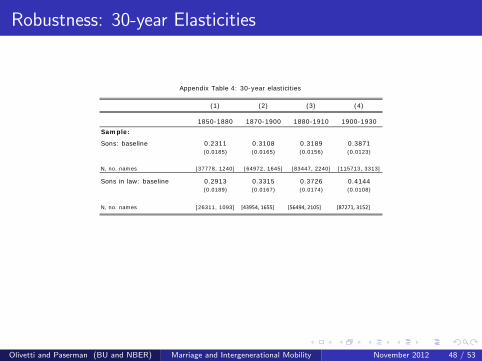
Robustness: 30-year Elasticities

(1) (2) (3) (4)

1850-1880 1870-1900 1880-1910 1900-1930Sample:

Sons: baseline 0.2311 0.3108 0.3189 0.3871(0.0185) (0.0165) (0.0156) (0.0123)

N, no. names [37778, 1240] [64972, 1645] [83447, 2240] [115713, 3313]

Sons in law: baseline 0.2913 0.3315 0.3726 0.4144(0.0189) (0.0167) (0.0174) (0.0108)

N, no. names [26311, 1093] [43954, 1655] [56494, 2105] [87271, 3152]

Appendix Table 4: 30-year elasticities


Mechanisms: Fertility and Birth Order

(1) (2) (3) (4) (5)

1850-1870 1860-1880 1880-1900 1900-1920 1910-1930

Baseline 0.3500 0.3133 0.3440 0.4953 0.4760(0.0239) (0.0200) (0.0166) (0.0152) (0.0118)

Control for number of siblings 0.2836 0.2735 0.3444 0.5024 0.4740(0.0255) (0.0214) (0.0168) (0.0157) (0.0121)

Control for birth order 0.3277 0.2860 0.3433 0.4974 0.4642(0.0247) (0.0207) (0.0166) (0.0154) (0.0119)

N, no. names (baseline) [37077, 1182] [50847, 1478] [80255, 2234] [109079, 3253][122468, 3720]

Baseline 0.3402 0.4009 0.3992 0.4932 0.4136(0.0213) (0.0191) (0.0183) (0.0131) (0.0100)

Control for number of siblings 0.2920 0.3044 0.3949 0.4651 0.3815(0.0239) (0.0210) (0.0190) (0.0140) (0.0109)

Control for birth order 0.3289 0.3659 0.3962 0.4734 0.3951(0.0215) (0.0197) (0.0184) (0.0133) (0.0104)

N, no. names (baseline) [23280, 976] [30081, 1376] [45804, 2063] [68439, 2888] [79314, 3326]

Table 10. Fertility and Birth order

A: Fathers-Sons



Mechanisms: Migration

(1) (2) (3) (4) (5)

1850-1870 1860-1880 1880-1900 1900-1920 1910-1930

Baseline 0.3500 0.3133 0.3440 0.4953 0.4760(0.0239) (0.0200) (0.0166) (0.0152) (0.0118)

Control for immigrant status 0.2992 0.2769 0.3247 0.4705 0.4659(0.0235) (0.0198) (0.0165) (0.0151) (0.0118)

Control for internal migrant status 0.2984 0.2766 0.3249 0.4708 0.4667(0.0235) (0.0198) (0.0164) (0.0151) (0.0118)

Control for immigrant status and father's 0.2367 0.2883 0.4420 0.4368(0.0195) (0.0163) (0.0150) (0.0117)

Control for internal migrant status and father's 0.2328 0.2862 0.4387 0.4342(0.0195) (0.0163) (0.0150) (0.0117)


Table 11. Immigration and Internal Migration

A: Fathers-Sons


Mechanisms: Migration

Baseline 0.3402 0.4009 0.3992 0.4932 0.4136(0.0213) (0.0191) (0.0183) (0.0131) (0.0100)

0.2720 0.3625 0.3676 0.4773 0.4086Control for immigrant status (0.0211) (0.0190) (0.0182) (0.0131) (0.0101)

0.2722 0.3619 0.3640 0.4733 0.4043Control for internal migrant status (0.0211) (0.0190) (0.0182) (0.0131) (0.0100)

0.3254 0.3122 0.4433 0.3815Control for immigrant status and father's (0.0188) (0.0180) (0.0131) (0.0101)

0.3215 0.3051 0.4372 0.3743Control for internal migrant status and father's (0.0188) (0.0180) (0.0130) (0.0100)




Mechanisms: Within-Region Analysis

(1) (2) (3) (4) (5)

1850-1870 1860-1880 1880-1900 1900-1920 1910-1930

All 0.3500 0.3133 0.3440 0.4953 0.4760(0.0239) (0.0200) (0.0166) (0.0152) (0.0118)

Northeast 0.2948 0.2539 0.1677 0.2187 0.1918(0.0383) (0.0337) (0.0310) (0.0279) (0.0224)

Midwest 0.1499 0.2521 0.2677 0.2771 0.2701(0.0468) (0.0368) (0.0315) (0.0279) (0.0230)

South 0.4593 0.1591 0.2878 0.3081 0.3641(0.0564) (0.0337) (0.0311) (0.0293) (0.0229)

N, no. names (all) [37077, 1182] [50847, 1478] [80255, 2234] [109079, 3253][122468, 3720]N, no. names (northeast) [11461, 580] [14846, 672] [19327, 727] [23818, 891] [29959, 1040]N, no. names (midwest) [7091, 442] [12713, 629] [25372, 1039] [35418, 1406] [38069, 1589]

N, no. names (south) [7709, 474] [11481, 607] [16570, 973] [23490, 1558] [30305, 1965]

Table 13. Intergenerational Elasticities 1850-1930. By Region of Birth.

A: Fathers-Sons


Mechanisms: Within-Region Analysis

All 0.3402 0.4009 0.3992 0.4932 0.4136(0.0213) (0.0191) (0.0183) (0.0131) (0.0100)

Northeast 0.2014 0.2221 0.3111 0.2743 0.2100(0.0380) (0.0382) (0.0409) (0.0333) (0.0261)

Midwest 0.3471 0.3811 0.3289 0.3371 0.3015(0.0520) (0.0353) (0.0337) (0.0238) (0.0183)

South 0.3975 0.3303 0.3192 0.4649 0.3791(0.0478) (0.0286) (0.0306) (0.0252) (0.0178)

N, no. names (all) [23280, 976] [30081, 1376] [45804, 2063] [68439, 2888] [79314, 3326]N, no. names (northeast) [6602, 448] [8102, 559] [9741, 602] [12819, 769] [16865, 923]N, no. names (midwest) [4877, 354] [7883, 586] [14957, 964] [22529, 1340] [24911, 1457]N, no. names (south) [5337, 408] [7200, 587] [10413, 926] [16556, 1335] [21104, 1625]



in the name of the father: marriage and intergenerational ... 1. summary statistics for...

Documents