In Search of Distress Risk

John Y. Campbell, Jens Hilscher, and Jan Szilagyi1

First draft: October 2004This version: December 2, 2004

1Corresponding author: John Y. Campbell, Department of Economics, Littauer Center213, Harvard University, Cambridge MA 02138, USA, and NBER. Tel 617-496-6448, emailjohn_campbell@harvard.edu. This material is based upon work supported by the National Sci-ence Foundation under Grant No. 0214061 to Campbell. We would like to thank Robert Jarrow andDon van Deventer of Kamakura Risk Information Services (KRIS) for providing us with bankruptcydata and Stuart Gilson, John Griffin, Scott Richardson, and seminar participants at HumboldtUniversität zu Berlin, HEC Paris, and the University of Texas for helpful discussion.

Abstract

This paper explores the determinants of corporate bankruptcy and the pricingof Þnancially distressed stocks using US data over the period 1963 to 1998. Firmswith higher leverage, lower proÞtability, lower market capitalization, lower past stockreturns, more volatile past stock returns, and lower cash holdings are more likelyto go into bankruptcy. When predicting bankruptcy at longer horizons, marketcapitalization, the most persistent predictor, becomes relatively more signiÞcant. Ourmodel captures much of the time variation in the US bankruptcy rate. Distressedstocks have delivered anomalously low returns during this period. They have lowerreturns but much higher standard deviations, market betas, and loadings on valueand small-cap risk factors than stocks with low bankruptcy risk. These Þndings areinconsistent with the conjecture that the value and size effects are compensation forthe risk of Þnancial distress.

1 Introduction

The concept of Þnancial distress is often invoked in the asset pricing literature toexplain otherwise anomalous patterns in the cross-section of stock returns. Theidea is that certain companies have an elevated risk that they will fail to meet theirÞnancial obligations, and investors charge a premium for bearing this risk.2

While this idea has a certain plausibility, it leaves a number of basic questionsunanswered. First, how do we measure the failure to meet Þnancial obligations?Second, how do we measure the probability that a Þrm will fail to meet its Þnancialobligations? Third, even if we have answered these questions and thereby constructedan empirical measure of Þnancial distress, is it the case that the stock prices ofÞnancially distressed companies move together in response to a common risk factor?Finally, what returns have Þnancially distressed stocks provided historically? Is thereany evidence that Þnancial distress risk carries a premium?

In this paper we adopt a relatively atheoretical econometric approach to measureÞnancial distress. We say that a Þrm fails to meet Þnancial obligations if it entersbankruptcy under either Chapter 7 or Chapter 11. That is, we ignore the possibilitythat a Þrm may avoid bankruptcy by negotiating a debt restructuring out of court(Gilson, John, and Lang 1990, Gilson 1997). We measure the probability of bank-ruptcy by estimating a hazard model using a logit speciÞcation, following Shumway(2001), Chava and Jarrow (2002), and others.

We extend the previous literature by considering a wide range of explanatoryvariables, including both accounting and equity-market variables, and by explicitlyconsidering how the optimal speciÞcation varies with the horizon of the forecast.Some papers on bankruptcy concentrate on predicting the event that a bankruptcywill occur during the next month. Over such a short horizon, it should not besurprising that the recent return on a Þrm�s equity is a powerful predictor, but thismay not be very useful information if it is relevant only in the extremely short run,just as it would not be useful to predict a heart attack by observing a person dropping

2Chan and Chen (1991), for example, attribute the size premium to the prevalence of �marginalÞrms� in small-stock portfolios, and describe marginal Þrms as follows: �They have lost marketvalue because of poor performance, they are inefficient producers, and they are likely to have highÞnancial leverage and cash ßow problems. They are marginal in the sense that their prices tend tobe more sensitive to changes in the economy, and they are less likely to survive adverse economicconditions.� Fama and French (1996) use the term �relative distress� in a similar fashion.

1

to the ßoor clutching his chest. We also explore time-series variation in the numberof bankruptcies, and ask how much of this variation is explained by changes over timein the variables that predict bankruptcy at the Þrm level.

Our empirical work begins with a bankruptcy indicator from Kamakura RiskInformation Services (KRIS), used by Chava and Jarrow (2002), which includes allbankruptcy Þlings in the Wall Street Journal Index, the SDC database, SEC Þlingsand the CCH Capital Changes Reporter. The data cover the months from January1963 until the end of 1998. We merge this dataset with Þrm level accounting datafrom COMPUSTAT as well as monthly and daily equity price data from CRSP. Thisgives us about 800 bankruptcies, and predictor variables for 1.3 million Þrm months.

We start by estimating a basic speciÞcation used by Shumway (2001) and similarto that of Chava and Jarrow (2002). The model includes both equity market andaccounting data. From the equity market, we measure the excess stock return of eachcompany over the past month, the volatility of daily stock returns over the past threemonths, and the market capitalization of each company. From accounting data, wemeasure net income as a ratio to assets, and total leverage as a ratio to assets.

From this starting point, we make a number of contributions to the prediction ofcorporate bankruptcy. First, we explore some sensible modiÞcations to the variableslisted above. SpeciÞcally, we show that scaling net income and leverage by the marketvalue of assets rather than the book value, adding further lags of stock returns andnet income, and including dummies for missing data can improve the explanatorypower of the benchmark regression.

Second, we explore some additional variables and Þnd that corporate cash holdingsand the market-book ratio also offer a marginal improvement. In a related exercisewe construct a measure of distance to default, based on the practitioner model ofKMV (Crosbie and Bohn 2001) and ultimately on the structural bankruptcy modelof Merton (1974). We Þnd that this measure adds relatively little explanatory powerto the reduced-form variables already included in our model.

Third, we examine what happens to our speciÞcation as we increase the horizonat which we are trying to predict bankruptcy. Consistent with our expectations,we Þnd that our most persistent forecasting variable, market capitalization, becomesrelatively more important as we predict bankruptcy further into the future.

Fourth, we study time-variation in the number of bankruptcies. We compare the

2

realized frequency of bankruptcy to the predicted frequency over time. Althoughthe model underpredicts the frequency of bankruptcy in the 1980s and overpredictsit in the 1990s, the model Þts the general time pattern quite well. We show thatmacroeconomic variables, in particular the default yield spread and the term spread,can be used to capture some of the residual time variation in the bankruptcy rate.

Finally, we explore the risks and average returns on portfolios of Þrms sorted byour Þtted probability of bankruptcy. We Þnd that Þrms with a high probability ofbankruptcy have high market betas and high loadings on the HML and SMB factorsproposed by Fama and French (1993, 1996) to capture the value and size effects.However they do not have high average returns, suggesting that the equity markethas not properly priced distress risk.

There is a large related literature that studies the prediction of corporate bank-ruptcy. The literature varies in choice of variables to predict bankruptcy and themethodology used to estimate the likelihood of bankruptcy. Altman (1968), Ohlson(1980), and Zmijewski (1984) use accounting variables to estimate the probability ofbankruptcy in a static model. Altman�s Z-score and Ohlson�s O-score have becomepopular and widely accepted measures of Þnancial distress. They are used, for ex-ample, by Dichev (1998), Griffin and Lemmon (2002), and Ferguson and Shockley(2003) to explore the risks and average returns for distressed Þrms.

Shumway (2001) estimates a hazard model at annual frequency and adds equitymarket variables to the set of scaled accounting measures used in the earlier literature.He points out that estimating the probability of bankruptcy in a static setting intro-duces biases and overestimates the impact of the predictor variables. This is becausethe static model does not take into account that a Þrm could have had high levelsof unfavorable indicators several periods before going into bankruptcy. Hillegeist,Cram, Keating and Lunstedt (2004) summarize equity market information by calcu-lating the probability of bankruptcy implied by the structural Merton model. Addingthis to accounting data increases the accuracy of bankruptcy prediction within theframework of a hazard model. Chava and Jarrow (2002) estimate hazard models atboth annual and monthly frequencies and Þnd that the accuracy of bankruptcy pre-diction is greater at a monthly frequency. They also compare the effects of accountinginformation across industries.

Duffie and Wang (2003) emphasize that the probability of bankruptcy depends onthe horizon one is considering. They estimate mean-reverting time series processesfor a macroeconomic state variable�personal income growth�and a Þrm-speciÞc

3

variable�distance to default. They combine these with a short-horizon bankruptcymodel to Þnd the marginal probabilities of default at different horizons. Usingdata from the US industrial machinery and instruments sector, they calculate termstructures of default probabilities. We conduct a similar exercise using a reduced-form econometric approach; we do not model the time-series evolution of the predictorvariables but instead directly estimate longer-term default probabilities.

The remainder of the paper is organized as follows. Section 2 describes theconstruction of the data set, outlier analysis and summary statistics. We comparethe distributions of the predictor variables for those observations where the Þrm wentbankrupt and all other observations. This section also considers the pattern of U.S.corporate bankruptcies over time.

Section 3 discusses our basic hazard speciÞcation, extensions to it, and the resultsfrom estimating the model at one-month and longer horizons. We Þnd that past stockreturn is less signiÞcant and market capitalization is more signiÞcant as the horizonincreases. This section also considers the stability of the model across industries,Þrms with high and low leverage, and large and small Þrms.

Section 4 considers the model�s Þt to the time-series pattern of bankruptices.When including year dummies to proxy for unobserved factors affecting bankruptcywe reject the null hypothesis that our model completely explains the aggregate historyof bankruptcy in the US. Comparing the predicted and realized frequencies ofbankruptcy, however, we Þnd that the model has considerable explanatory power forthis history.

Section 5 studies the return properties of equity portfolios formed on the Þttedvalue from our bankruptcy prediction model. We ask whether stocks with highbankruptcy probability have unusually high or low returns relative to the predictionsof standard cross-sectional asset pricing models such as the CAPM or the three-factorFama-French model. Section 6 concludes.

4

2 Data description

In order to estimate a hazard model of bankruptcies we need a bankruptcy indicatorand a set of explanatory variables. The bankruptcy indicator we use is taken fromChava and Jarrow (2002); it includes all bankruptcy Þlings in the Wall Street JournalIndex, the SDC database, SEC Þlings and the CCH Capital Changes Reporter. Theindicator is one in a month in which a Þrm Þled for bankruptcy under Chapter7 or Chapter 11, and zero otherwise; in particular, the indicator is zero if the Þrmdisappears from the dataset for some reason other than bankruptcy such as acquisitionor delisting. The data span the months from December 1963 through December 1998.

Table 1 summarizes the properties of the bankruptcy indicator. The Þrst columnshows the number of active Þrms for which we have data in each year; the secondcolumn shows the number of bankruptcies; and the third column reports the percent-age of active Þrms that went bankrupt in each year. This series is also illustratedin Figure 1. It is immediately apparent that bankruptcies were extremely rare untilthe late 1960�s. In fact, in the three years 1967�1969 there were no bankruptcies atall in our dataset. The bankruptcy rate increased in the early 1970�s, and then rosedramatically during the 1980�s to a peak of 1.7% in 1986. It remained high throughthe economic slowdown of the early 1990�s, but fell in the late 1990�s to levels onlyslightly above those that prevailed in the 1970�s.

Some of these changes through time are probably the result of changes in thelaw governing corporate bankruptcy in the 1970�s, and related Þnancial innovationssuch as the development of below-investment-grade public debt (junk bonds) in the1980�s and the advent of prepackaged bankruptcy Þlings in the early 1990�s (Tashjian,Lease, and McConnell 1996). Changes in corporate capital structure (Bernanke andCampbell 1988) and the riskiness of corporate activities (Campbell, Lettau, Malkiel,and Xu 2001) are also likely to have played a role, and one purpose of our investigationis to quantify the time-series effects of these changes.

In order to construct explanatory variables at the individual Þrm level, we com-bine quarterly accounting data from COMPUSTAT with monthly and daily equitymarket data from CRSP. From COMPUSTAT we construct a standard measure ofproÞtability: net income relative to total assets. Previous authors have measuredtotal assets at book value, but we Þnd better explanatory power when we measurethe equity component of total assets at market value by adding the book value ofliabilities to the market value of equities. We call this series NIMTA (Net Income

5

to Market-valued Total Assets) and the traditional series NITA (Net Income to TotalAssets). We also use COMPUSTAT to construct a measure of leverage: total lia-bilities relative to total assets. We again Þnd that a market-valued version of thisseries, deÞned as total liabilities divided by the sum of market equity and book liabil-ities, performs better than the traditional book-valued series. We call the two seriesTLMTA and TLTA, respectively. To these standard measures of proÞtability andleverage, we add a measure of liquidity, the ratio of a company�s cash and short-termassets to the market value of its assets (CASHMTA). We also calculate each Þrm�smarket-to-book ratio (MB).

In constructing these series we adjust the book value of assets to eliminate outliers,following the procedure suggested by Cohen, Polk, and Vuolteenaho (2003). Thatis, we add 10% of the difference between market and book equity to the book valueof total assets, thereby increasing book values that are extremely small, probablymismeasured, and create outliers when used as the denominators of Þnancial ratios.We also winsorize all variables at the 5th and 95th percentiles of their cross-sectionaldistributions. That is, we replace any observation below the 5th percentile with the5th percentile, and any observation above the 95th percentile with the 95th percentile.We are careful to adjust each company�s Þscal year to the calendar year and lag thedata by two months. This adjustment ensures that the accounting data are availableat the beginning of the month over which bankruptcy is measured. The Appendixto this paper describes the construction of these variables in greater detail.

We add several market-based variables to these two accounting variables. Wecalculate the monthly log excess return on each Þrm�s equity relative to the S&P 500index (EXRET), the standard deviation of each Þrm�s daily stock return over the pastthree months (SIGMA), and the relative size of each Þrm measured as the log ratioof its market capitalization to that of the S&P 500 index (RSIZE). In addition, weobtain historical yields on 6-month Treasury bills and 10-year Treasury bonds fromthe Federal Reserve Board, and historical yields on AAA and BAA rated corporatebonds from Amit Goyal�s website.3

Finally, we group all Þrms into four broad sectors using single-digit SIC codes.Industry 1 is miscellaneous (codes 1, 3, 6, 7, 9), industry 2 is manufacturing andminerals (codes 2, 4), industry 3 is transportation, communication and utilities (code5), and industry 4 is Þnance, insurance and real estate (code 8).

3The Federal Reserve data are at http://www.federalreserve.gov/releases/h15/data.htm and thecorporate bond data are at http://www.bus.emory.edu/AGoyal/.

6

2.1 Summary statistics

Table 2 summarizes the properties of our seven main explanatory variables. The Þrstpanel in Table 2 describes non-bankruptcy months and the second panel describes amuch smaller sample of bankruptcy months. We exclude months where any of theseven variables have missing values, leaving us with a sample of 1,281,426 observa-tions containing 796 bankruptcy events. We also illustrate the data in a series ofgraphs. Figures 2 through 8 each have two panels, one showing the distribution of anexplanatory variable in non-bankruptcy months, the other showing the distributionin the much smaller sample of bankruptcy months.

In interpreting these distributions, it is important to keep in mind that we weightevery Þrm-month equally. This has two important consequences. First, the distri-butions are dominated by the behavior of relatively small companies; value-weighteddistributions look quite different. Second, the distributions reßect the inßuence ofboth cross-sectional and time-series variation. The cross-sectional averages of severalvariables, in particular NIMTA, TLMTA, and SIGMA, have experienced signiÞcanttrends since 1963: SIGMA and TLMTA have trended up, while NIMTA has trendeddown. The downward trend in NIMTA is not just a consequence of the buoyantstock market of the 1990�s, because book-based net income, NITA, displays a similartrend. The inßuence of these trends is magniÞed by the growth in the number ofcompanies over time, which means that recent years have greater inßuence on thedistribution than earlier years.

These facts help to explain several features of Table 2. The mean level of NIMTA,for example, is only 0.002 or 0.2% per quarter in our dataset, 0.8% at an annual rate.This is three times lower than the median level of NIMTA because the distribution ofNIMTA is negatively skewed; it is also lower than the average level of NITA becausethe market value of equity is on average about twice the book value in our data.Nonetheless these measures of proÞtability are all strikingly low, reßecting the preva-lence of small, unproÞtable listed companies in recent years.4 The distribution ofNIMTA shown in Figure 2 has a large spike just above zero, a phenomenon noted byHayn (1995), suggesting that Þrms may be managing their earnings to avoid reportinglosses.5

4The value-weighted mean of NIMTA is three times the equal-weighted mean, reßecting thegreater proÞtability of large companies.

5There is a debate in the accounting literature about the interpretation of this spike. Burgstahlerand Dichev (1997) argue that it reßects earnings management, but Dechow, Richardson, and Tuna

7

The average value of EXRET is -0.012 or -1.2% per month. This extremely lownumber reßects both the underperformance of small stocks during the later part ofour sample period (the value-weighted mean is almost exactly zero), and the factthat we are reporting a geometric average excess return rather than an arithmeticaverage. The difference is substantial because individual stock returns are extremelyvolatile. The average value of the annualized Þrm-level volatility SIGMA is greaterthan 50%, again reßecting the strong inßuence of small Þrms and recent years in whichidiosyncratic volatility has been high (Campbell, Lettau, Malkiel, and Xu 2001).

A comparison of the top and bottom panels of Table 2, and inspection of Figures2�8, reveal that bankrupt Þrms have intuitive differences from the rest of the sample.In months immediately preceding a bankruptcy Þling, Þrms typically make losses (themean loss is 3.5% quarterly or 14% of market value of assets at an annual rate, andthe median loss is 4.7% quarterly or almost 19% at an annual rate); the value of theirdebts is extremely high relative to their assets (average leverage exceeds 75%, andmedian leverage exceeds 85%); they have experienced extremely negative returns overthe past month (the mean is -132% at an annual rate or -11% over a month, whilethe median is -208% at an annual rate or -17% over a month); and their volatilityis extraordinarily high (the mean is 99% and the median is 121%). Bankrupt Þrmsalso tend to be relatively small (almost 8 times smaller than other Þrms on average,and almost 12 times smaller at the median), and they have only about half as muchcash and short-term investments, in relation to the market value of assets, as non-bankrupt Þrms. Finally, the market-book ratio of bankrupt Þrms has a similarmean but a much higher standard deviation than the market-book ratio of otherÞrms. Figure 8 shows that almost 40% of Þrms have market-book ratios at the lowerwinsorization point, while 25% have market-book ratios at the upper winsorizationpoint. It appears that some Þrms go bankrupt after realized losses have driven downtheir book values relative to market values, while others go bankrupt after bad newsabout future prospects has driven down their market values relative to book values.

(2003) point out that discretionary accruals are not associated with the spike in the manner thatwould be expected if this interpretation is correct.

8

3 Estimating a hazard model for bankruptcy

The summary statistics in Table 2 show that bankrupt Þrms have a number of unusualcharacteristics. However the number of bankruptcy months is tiny compared to thenumber of other months, so it is not at all clear how useful these variables are inpredicting bankruptcy. Also, these characteristics are correlated with one anotherand we would like to know how to weight them optimally. Following Shumway (2001)and Chava and Jarrow (2002), we now estimate the probability of bankruptcy overthe next period using a logit model.

We assume that the marginal probability of bankruptcy over the next periodfollows a logistic distribution and is given by

Pt−1 (Yit = 1) =1

1 + exp (−α− βxi,t−1) (1)

where Yit is a bankruptcy indicator that is equal to one if the Þrm goes bankrupt inmonth t, and xi,t−1 is a vector of explanatory variables known at the end of the previ-ous month. A higher level of α+βxi,t−1 implies a higher probability of bankruptcy.

Table 3 reports logit regression results for various alternative speciÞcations. Incolumn 1 we follow Shumway (2001) and Chava and Jarrow (2002), and estimatea model with Þve standard variables: NITA, TLTA, EXRET, SIGMA, and RSIZE.This model measures assets in the conventional way, using annual book values fromCOMPUSTAT. It excludes Þrm age, a variable which Shumway (2001) consideredbut found to be insigniÞcant in predicting bankruptcy.

All Þve of the included variables in column 1 enter signiÞcantly and with theexpected sign. To get some idea of the relative impact of changes in the differentvariables we compute the effect on the score of a one-standard-deviation change ineach predictor variable. This effect is 0.29 for NITA, 0.96 for TLTA, 0.39 for EXRET,0.36 for RSIZE, and 0.91 for SIGMA. Thus movements in leverage and volatility aremore important for explaining bankruptcy than movements in proÞtability, past stockreturns, and Þrm size.

In column 2 we replace the traditional accounting ratios NITA and TLTA that usethe book value of assets, with our ratios NIMTA and TLMTA that use the marketvalue of assets. These measures are more sensitive to new information about Þrmprospects since equity values are measured using monthly market data rather than

9

quarterly accounting data. Column 2 appears to be an improved speciÞcation inseveral respects. The coefficient on proÞtability more than doubles and increasesits statistical signiÞcance, and the pseudo R2, a measure of Þt for the logit model,increases by 0.005. Interestingly, the coefficient on RSIZE becomes small and statis-tically insigniÞcant, suggesting that its role in column 1 was an artifact of our use ofaccounting data.

Column 2 has 5% more observations than column 1, because we no longer needto measure book values of assets in the COMPUSTAT dataset. Importantly, thenumber of bankruptcies increases by 3% from 737 to 762. Since bankruptcies are rareevents, it is important to include as many of them as we possibly can. Accordinglyin column 3 we expand the dataset further by relaxing the requirement that we beable to measure equity market volatility, SIGMA, over the past three months. Incases where this variable is missing, we create a dummy variable SIGMAMISS andenter it in the column 3 regression. This increases the number of observations byanother 1% and the number of bankruptcies by another 4% to 796. As one wouldexpect from these statistics, the dummy variable enters signiÞcantly as a bankruptcypredictor. Firms with intermittent equity trading over the past three months aremore likely to fail our test for valid construction of equity volatility, and are also morelikely to go bankrupt. The magnitude of the SIGMAMISS coefficient implies thatmissing volatility is equivalent to volatility about 1.5 standard deviations above thecross-sectional mean.

So far we have used only the information in the most recent values of proÞtability,leverage, excess returns, and volatility. An obvious question is whether lagged valueshave some additional explanatory power. One might expect that a long history oflosses or a sustained decline in stock market value would be a better predictor ofbankruptcy than one large quarterly loss or a sudden stock price decline in a singlemonth. Exploratory regressions with lagged values conÞrm that lags of NIMTA andEXRET enter signiÞcantly, while lags of the other variables do not. As a reasonablesummary, we impose geometrically declining weights on these lags. We construct

NIMTAAVGt−1,t−12 =1− φ31− φ12

¡NIMTAt−1,t−3 + ...+ φ9NIMTAt−9,t−12

¢,(2)

EXRETAV Gt−1,t−12 =1− φ1− φ12 (EXRETt−1 + ...+ φ11EXRETt−12), (3)

10

where the coefficient φ = 2−13 , implying that the weight is halved each quarter. The

data suggest that this parsimonious speciÞcation captures almost all the predictabil-ity obtainable from lagged proÞtability and stock returns. Column 4 of Table 3reports the regression results using this speciÞcation, Þnding an improvement in theexplanatory power of stock returns. This speciÞcation causes a further decline in theimportance of market capitalization, whose coefficient actually changes sign.

In column 5 we add two other variables that might be relevant for bankruptcyprediction. The ratio of cash and short-term investments to the market value oftotal assets, CASHMTA, captures the liquidity of the Þrm. A Þrm with a highCASHMTA ratio has liquid assets available to make interest payments, and thusmay be able to postpone bankruptcy with the possibility of avoiding it altogether ifcircumstances improve. The market to book ratio, MB, captures the relative valueplaced on the Þrm�s equity by stockholders and by accountants. Our proÞtabilityand leverage ratios use market value; if book value is also relevant, then MB mayenter the regression as a correction factor, increasing the probability of bankruptcywhen market value is unusually high relative to book value.6 Column 5 supportsboth these hypotheses.

Finally, in column 6 we compare our reduced-form model with the structuralapproach of KMV (Crosbie and Bohn 2001), based on the structural bankruptcymodel of Merton (1974). We construct �distance to default�, DD, applying a standardformula given in the Appendix. This formula requires an estimate of the volatilityof the Þrm�s asset value, and we make the assumption that asset volatility equalsequity volatility. For Þrms with relatively safe debt, this assumption will understatethe distance to default. Although our DD measure does predict default with thetheoretically expected sign in a univariate logit regression, its explanatory poweris much lower than our reduced-form approach (the pseudo R2 is only about 8%).Column 6 shows that DD adds relatively little explanatory power to the reduced-form variables already included in our model, and in fact enters our multivariateregression with the wrong sign.

6Chacko, Hecht, and Hilscher (2004) discuss the measurement of credit risk when the market-to-book ratio is inßuenced both by cash ßow expectations and discount rates.

11

3.1 Forecasting bankruptcy at long horizons

At the one month horizon our best speciÞcation captures about 30% of the variation inbankruptcy risk. We now ask what happens as we try to predict bankruptcies furtherinto the future. In Table 4 we estimate the conditional probability of bankruptcyin six months, one, two and three years. We again assume a logit speciÞcation butallow the coefficients on the variables to vary over time. In particular we assumethat the probability of bankruptcy in j months, conditional on survival in the datasetfor j − 1 months, is given by

Pt−1 (Yi,t−1+j = 1 | Yi,t−2+j = 0) = 1

1 + exp¡−αj − βjxi,t−1¢ . (4)

Note that this assumption does not imply a cumulative probability of bankruptcythat is logit. If the probability of bankruptcy in j months did not change with thehorizon j, that is if αj = α and βj = β, and if Þrms exited the dataset only throughbankruptcy, then the cumulative probability of bankruptcy over the next j periodswould be given by 1 − (exp (−α− βxi) /(1 + exp (−α− βxi))j, which no longer hasthe logit form. Variation in the parameters with the horizon j, and exit from thedataset through mergers and acquisitions, only make this problem worse. In principlewe could compute the cumulative probability of bankruptcy by estimating models foreach horizon j and integrating appropriately; or by using our one-period model andmaking auxiliary assumptions about the time-series evolution of the predictor vari-ables in the manner of Duffie and Wang (2003). We do not pursue these possibilitieshere, concentrating instead on the conditional probabilities of default at particulardates in the future.

As the horizon increases in Table 4, the coefficients, signiÞcance levels, and overallÞt of the logit regression decline as one would expect. Even at three years, however,almost all the variables remain statistically signiÞcant. The distance to defaultDD enters the regression with the theoretically expected negative sign at horizonsof two and three years, but it is statistically insigniÞcant; this result is particularlydisappointing since DD is designed to measure bankruptcy risk at a medium-termhorizon of one year.

Two predictor variables are particularly important at long horizons. The coef-Þcient on the market-to-book ratio MB is remarkably stable, and the coefficient onrelative size RSIZE becomes increasingly signiÞcant with the expected negative sign

12

as the horizon increases. These results imply that the most persistent attributesof a Þrm, its market capitalization and market-to-book ratio, become increasinglyimportant measures of Þnancial distress at long horizons.

In the top panel of Table 4 the number of observations and number of bankruptciesvary with the horizon, because increasing the horizon forces us to drop observationsat both the beginning and end of the dataset. Bankruptcies that occur within theÞrst j months of the sample cannot be related to the condition of the Þrm j monthspreviously, and the last j months of the sample cannot be used to predict bankruptciesthat may occur after the end of the sample. Also, many Þrms exit the dataset forother reasons between dates t− 1 and t− 1 + j. In the bottom panel of Table 4 westudy a subset of Þrms for which data are available at all the different horizons. Thisallows us to compare R2 statistics directly across horizons. We obtain very similarresults to those in the top panel, suggesting that variation in the available data is notresponsible for our Þndings.

3.2 Robustness checks

We have explored industry effects on the bankruptcy models estimated in Tables 3and 4. The Shumway (2001) and Chava-Jarrow (2002) speciÞcation in column 1of Table 3 appears to behave somewhat differently in the Þnance, insurance, andreal estate (FIRE) sector. That sector has a lower intercept and a more negativecoefficient on proÞtability. However there is no clear evidence of sector effects in themarket-based speciÞcations estimated in the other columns of Table 3.

We have also used market capitalization and leverage as interaction variables, totest the hypotheses that other explanatory variables enter differently for small orhighly indebted Þrms than for other Þrms. We have found no clear evidence thatsuch interactions are important.

13

4 Matching the time series of bankruptcies

As we noted earlier, there is dramatic variation in the bankruptcy rate over time.Figure 1 shows the bankruptcy rate rising from an average of 0.3% in the 1960�s and1970�s to almost 1.7% in 1986. In this section, we ask how well our model Þts thispattern. We Þrst calculate the Þtted probability of bankruptcy for each companyin our dataset using the coefficients from the best Þtting regression in Table 3. Wethen average over all the predicted probabilities for active companies in each monthto obtain a prediction of the aggregate bankruptcy rate.

Figure 9 shows annual averages of predicted and realized bankruptcies. Ourmodel captures much of the broad variation in bankruptcy over time, including thestrong and long-lasting increase in the 1980�s and cyclical spikes in the mid-1970�sand early 1990�s. However it somewhat overpredicts these spikes and rises in the1980�s much more slowly than actual bankruptcies. In the worst performing yearof 1986, the model underestimates the bankruptcy rate by about one half. Also,the model tends to predict more bankruptcies than actually occurred throughout the1990�s.

As an alternative way to understand the time-series variation that is not capturedby our basic model, we augment that model by including year dummies that shiftthe baseline probability of bankruptcy from one year to the next. We restrict ourattention to the period since 1975 because of the rarity of bankruptcies in earlieryears.

Figures 10 and 11 plot the demeaned year dummies estimated from a model withonly these dummies (Figure 10) and a model that also includes our standard set ofexplanatory variables (Figure 11). We overwhelmingly reject the hypothesis thatthe year dummies are all equal�that is, that time effects can be omitted from themodel�although the Wald statistic for this test does fall from 172 in Figure 10 to129 in Figure 11, implying that our model captures some of the time-variation inbankruptcies.

To show which years have anomalous variation in bankruptcies, Figures 10 and11 also plot a two-standard-deviation conÞdence interval for each demeaned yeardummy, constructed under the null hypothesis that all year dummies are equal. TheconÞdence interval is signiÞcantly narrower in later years because the number of Þrm-level observations increases over time. The model with only year dummies has a

14

standard deviation of 0.63 for the dummies and displays unusually high bankruptcyrisk throughout the 1980�s and early 1990�s, whereas the model that uses Þrm-levelmarket and accounting data has a smaller standard deviation of 0.45 and relies onvariation in the year dummies primarily in the early 1980�s and the late 1990�s. It ispossible that positive year dummies in the early 1980�s reßect the creation of the junkbond market in that period, and that negative year dummies in the late 1990�s reßectthe increased tendency of Þrms to restructure their debt without entering bankruptcy.

4.1 Macroeconomic effects

One interpretation of time effects is that they result from changes in the state ofthe macroeconomy. Duffie and Wang (2003), for example, give an important role tothe growth rate of industrial production in their multi-period bankruptcy model. Inorder to explore macroeconomic effects, we Þrst added NBER recession dummies toour best Þtting model for the period since 1976, both in levels and interacted with theother coefficients to allow a regime change in bankruptcy risk during a recession. Weused both contemporaneous and six-month lagged dummies to capture the possibilitythat bankruptcies respond to macroeconomic conditions with a lag. However noneof these variables entered the model signiÞcantly.

We obtain more promising results when we allow for an effect of interest rates onbankruptcy risk. We measure the default yield spread between BAA and AAA rateddebt, DFY, and the term spread between 10-year Treasury bonds and six-monthTreasury bills, TMS. If we add these variables directly to the regression, withoutinteractions, they enter signiÞcantly. If we allow them to interact with the othervariables in the model, the interactions of DFY with relative size and leverage aresigniÞcant and drive out the direct effect of DFY, while the interaction of TMS withleverage is signiÞcant and again drives out the direct effect of TMS.

Table 5 reports the results. Column 1 shows that an increase in the default yieldspread reduces bankruptcy risk for highly leveraged Þrms and increases it for smallÞrms. This is consistent with the view that a high default yield spread is a signal ofa credit crunch, which tends to dry up credit to small Þrms and increase the averagequality of Þrms that do receive credit. Column 2 shows that an increase in the slopeof the yield curve reduces bankruptcy risk for highly leveraged Þrms. Since the yieldspread usually rises when short-term interest rates fall, this may reßect relief to highlyindebted Þrms with ßoating-rate debt when short rates decline.

15

The default yield spread is particularly successful at reducing the importance oftime dummies in our model. When we include only DFY interacted with relative sizeand leverage, and not the level of DFY, the Wald test statistic for the signiÞcance ofthe time dummies falls to 66 even though the regression includes no pure time-seriesvariables.

5 Risks and average returns on distressed stocks

We now turn our attention to the asset pricing implications of our bankruptcy model.Recent work on the distress premium has tended to use either traditional risk indicessuch as the Altman Z-score or Ohlson O-score (Dichev 1998, Griffin and Lemmon2002, Ferguson and Shockley 2003) or the distance to default measure of KMV (Vas-salou and Xing 2004). To the extent that our reduced-form model more accuratelymeasures the risk of bankruptcy at short and long horizons, we can more accuratelymeasure the premium that investors receive for holding distressed stocks.

Before presenting the results, we ask what results we should expect to Þnd. On theone hand, if investors accurately perceive the risk of bankruptcy they may demanda premium for bearing it. The frequency of bankruptcy shows strong variationover time, as illustrated in Figure 1; even if much of this time-variation is explainedby time-variation in our Þrm-level predictive variables, it still generates commonmovement in stock returns that might command a premium.

Of course, a risk can be pervasive and still be unpriced. If the standard imple-mentation of the CAPM is exactly correct, for example, then each Þrm�s risk is fullycaptured by its covariation with the market portfolio of equities, and bankruptcy riskis unpriced to the extent that it is uncorrelated with that portfolio. However it seemsplausible that bankruptcies may be correlated with declines in unmeasured compo-nents of wealth such as human capital (Fama and French 1996) or debt securities(Ferguson and Shockley 2003), in which case bankruptcy risk will carry a positiverisk premium.7 This expectation is consistent with the high bankruptcy risk of small

7Fama and French (1996) state the idea particularly clearly: �Why is relative distress a statevariable of special hedging concern to investors? One possible explanation is linked to humancapital, an important asset for most investors. Consider an investor with specialized human capitaltied to a growth Þrm (or industry or technology). A negative shock to the Þrm�s prospects probablydoes not reduce the value of the investor�s human capital; it may just mean that employment in the

16

Þrms that have depressed market values, since small value stocks are well known todeliver high average returns.

An alternative possibility is that investors fail to understand the relation betweenour predictive variables and bankruptcy risk, and so do not discount the prices ofhigh-risk stocks enough to offset their bankruptcy probability. This investor failurecould be consistent with rational learning through the sample period after the increasein bankruptcies during the 1970�s, or it could be a deeper failure of the sort postulatedby behavioral Þnance. In either case we will Þnd that bankruptcy risk appears tocommand a negative risk premium during our sample period. This expectation isconsistent with the high bankruptcy risk of volatile stocks, since Ang, Hodrick, Xing,and Zhang (2004) have recently found negative average returns for stocks with highidiosyncratic volatility.

We measure the premium for Þnancial distress by sorting stocks according totheir bankruptcy probabilities, estimated using the 12-month-ahead model of Table4. Each January from 1976 through 1998, we form ten equally weighted portfoliosof stocks that fall in different regions of the bankruptcy risk distribution. We holdthese portfolios for a year, allowing the weights to drift with returns within theyear rather than rebalancing monthly, in order to minimize turnover costs and theeffects of bid-ask bounce.8 Our portfolios contain stocks in percentiles 0�5, 5�10,10�20, 20�40, 40�60, 60�80, 80�90, 90�95, 95�99, and 99�100 of the bankruptcy riskdistribution. This portfolio construction procedure pays greater attention to thetails of the distribution, where the distress premium is likely to be more relevant, andparticularly to the most distressed Þrms.

Because we are studying the returns to distressed stocks, it is important to handlecarefully the returns to stocks that are delisted and thus disappear from the CRSPdatabase. In many cases CRSP reports a delisting return for the Þnal month ofthe Þrm�s life; we have 8,243 such delisting returns in our sample and we use them

Þrm will grow less rapidly. In contrast, a negative shock to a distressed Þrm more likely implies anegative shock to the value of human capital since employment in the Þrm is more likely to contract.Thus, workers with specialized human capital in distressed Þrms have an incentive to avoid holdingtheir Þrms� stocks. If variation in distress is correlated across Þrms, workers in distressed Þrmshave an incentive to avoid the stocks of all distressed Þrms. The result can be a state-variable riskpremium in the expected returns of distressed stocks.� (p.77).

8In the Þrst version of this paper we calculated returns on portfolios rebalanced monthly, andobtained similar results to those reported here.

17

where they are available. Otherwise, we use the last available full-month return inCRSP. In some cases this effectively assumes that our portfolios sell distressed stocksat the end of the month before delisting, which imparts an upward bias to the returnson distressed-stock portfolios (Shumway 1997, Shumway and Warther 1999).9 Weassume that the proceeds from sales of delisted stocks are reinvested in each portfolioin proportion to the weights of the remaining stocks in the portfolio. In a few cases,stocks are delisted and then re-enter the database, but we do not include these stocksin the sample after the Þrst delisting. We treat Þrms that enter bankruptcy asequivalent to delisted Þrms, even if CRSP continues to report returns for these Þrms.That is, our portfolios sell stocks of companies that enter bankruptcy and we use thelatest available CRSP data to calculate a Þnal return on such stocks.

Table 6 reports the results. Each portfolio corresponds to one column of thetable. The top panel reports average monthly returns in excess of the market, witht statistics below in parentheses, and then alphas with respect to the CAPM, thethree-factor model of Fama and French (1993), and a four-factor model proposed byCarhart (1997) that also includes a momentum factor. The bottom panel reportsestimated factor loadings for excess returns on the three Fama-French factors, againwith t statistics, and the standard deviation of each portfolio�s excess return. Figures12 and 13 graphically summarize the behavior of factor loadings and alphas.

The average returns in the Þrst row of Table 6 are monotonically declining inbankruptcy risk, with a spread of 1.0% per month between the lowest-risk and highest-risk portfolios. The excess returns for low-risk portfolios are signiÞcantly positive,but those for high-risk portfolios are statistically insigniÞcant because of their highvolatility. While the low-risk portfolios have monthly standard deviations between2.0 and 2.5%, the highest-risk portfolio has a standard deviation of 11.2% and thenext portfolio has a standard deviation of 7.0%.

There is striking variation in factor loadings across the portfolios in Table 6. Thelow-risk portfolios have negative market betas for their excess returns (that is, betasless than one for their raw returns), and small or negative loadings on the value factorHML. The high-risk portfolios have positive market betas for their excess returns, andloadings greater than one on HML. Because the portfolios are equally weighted, theyall have high loadings on the size factor SMB, but the loadings increase dramaticallywith bankruptcy risk. This reßects the role of market capitalization in predicting

9In the Þrst version of this paper we did not use CRSP delisting returns. The portfolio resultswere similar to those reported here.

18

bankruptcies at medium and long horizons.

These factor loadings imply that when we correct for risk using either the CAPMor the Fama-French three-factor model, we worsen the anomalous poor performanceof distressed stocks rather than correcting it. The spread in CAPM alphas betweenthe lowest-risk and highest-risk portfolios is 1.2% per month, and the spread in Fama-French alphas is 1.8% per month. The poor performance of distressed stocks, andnot just the good performance of relatively safe stocks, is statistically signiÞcant whenwe use the Fama-French model.

One of the variables that predicts bankruptcy in our model is recent past return.This suggests that distressed stocks have negative momentum, which might explaintheir low average returns. To control for this, Table 6 also reports alphas from theCarhart (1997) four-factor model including a momentum factor. The negative alphasfor distressed stocks improve slightly, but remain statistically signiÞcant.

Overall, these results are discouraging for the view that distress risk is positivelypriced in the US stock market. We Þnd that stocks with a high risk of bankruptcyhave low average returns, despite their high loadings on small-cap and value riskfactors.

6 Conclusion

This paper makes two main contributions to the literature on Þnancial distress. First,we carefully implement a reduced-form econometric model to predict bankruptcy atshort and long horizons. Our best model has greater explanatory power than theexisting state-of-the-art models estimated by Shumway (2001) and Chava and Jarrow(2002), and includes additional variables with sensible economic motivation. We be-lieve that models of the sort estimated here have meaningful empirical advantages overthe bankruptcy risk scores proposed by Altman (1968) and Ohlson (1980). WhileAltman�s Z-score and Ohlson�s O-score were seminal early contributions, better mea-sures of bankruptcy risk are available today. We have also presented evidence thatbankruptcy risk cannot be adequately summarized by a measure of distance to de-fault inspired by Merton�s (1974) pioneering structural model of bankruptcy. Whileour distance to default measure is not exactly the same as those used by Crosbie andBohn (2001) and Vassalou and Xing (2004), we believe that this result will be robust

19

to alternative measures of distance to default.

Second, we show that stocks with a high risk of bankruptcy tend to deliver anom-alously low average returns. We sort stocks by our 12-month-ahead estimate ofbankruptcy risk. Distressed portfolios, containing stocks with high estimated bank-ruptcy risk, have low average returns but high standard deviations, market betas,and loadings on Fama and French�s (1993) small-cap and value risk factors. Thus,from the perspective of any of the leading empirical asset pricing models, these stockshave negative alphas. This result is a signiÞcant challenge to the conjecture thatthe value and size effects are proxies for a distress premium. More generally, it is achallenge to standard models of rational asset pricing in which the structure of theeconomy is stable and well understood by investors.

This version of our paper is preliminary, and we plan to expand our empiricalinvestigation in several directions. One particularly important question is whetherthe determinants of bankruptcy risk are stable over time. Our best model has a goodin-sample Þt, but we would like to show that it predicts bankruptcy when estimatedusing only data available up to each point of time. Rolling estimates of the modelwill also allow us to construct portfolios of distressed stocks using contemporaneouslyavailable information about the determinants of bankruptcy.

It should be possible to reÞne our understanding of the bankruptcy risk anomalyby sorting stocks on other characteristics. Our results are consistent with the Þnd-ings of Dichev (1998), who uses Altman�s Z-score and Ohlson�s O-score to measureÞnancial distress. Vassalou and Xing (2004) use distance to default as an alternativedistress measure; they Þnd some evidence that distressed stocks have higher returns,but this evidence comes entirely from small value stocks. Griffin and Lemmon (2002),using O-score to measure distress, show that distressed growth stocks have particu-larly low returns. This literature suggests that it will be fruitful to sort stocks on sizeand book-market ratio as well as bankruptcy risk, in order to identify which types ofdistressed stocks have positive or negative abnormal returns.

One possible explanation of the bankruptcy risk anomaly is that it results fromthe preferences of institutional investors, together with a shift of assets from indi-viduals to institutions during our sample period. Kovtunenko and Sosner (2003)have documented that institutions prefer to hold proÞtable stocks, and that this pref-erence helped institutional performance during the 1980�s and 1990�s because prof-itable stocks outperformed the market. It is possible that the strong performanceof proÞtable stocks in this period was endogenous, the result of increasing demand

20

for these stocks by institutions. If institutions more generally prefer stocks with lowbankruptcy risk, and tend to sell stocks that enter Þnancial distress, then a similarmechanism could drive our results. This hypothesis can be tested by relating the per-formance of distressed stocks over time to the changing institutional share of equityownership.

21

Appendix

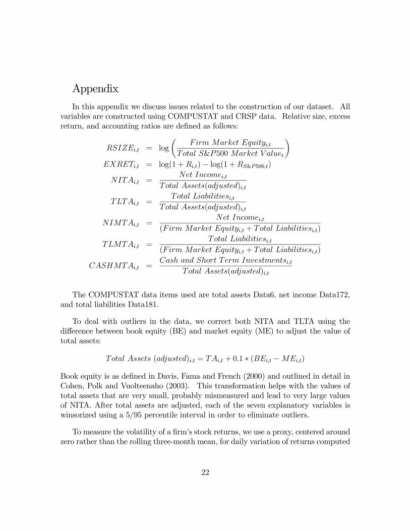
In this appendix we discuss issues related to the construction of our dataset. Allvariables are constructed using COMPUSTAT and CRSP data. Relative size, excessreturn, and accounting ratios are deÞned as follows:

RSIZEi,t = log

µFirm Market Equityi,t

Total S&P500 Market V aluet

¶EXRETi,t = log(1 +Ri,t)− log(1 +RS&P500,t)NITAi,t =

Net Incomei,tTotal Assets(adjusted)i,t

TLTAi,t =Total Liabilitiesi,t

Total Assets(adjusted)i,t

NIMTAi,t =Net Incomei,t

(Firm Market Equityi,t + Total Liabilitiesi,t)

TLMTAi,t =Total Liabilitiesi,t

(Firm Market Equityi,t + Total Liabilitiesi,t)

CASHMTAi,t =Cash and Short Term Investmentsi,t

Total Assets(adjusted)i,t

The COMPUSTAT data items used are total assets Data6, net income Data172,and total liabilities Data181.

To deal with outliers in the data, we correct both NITA and TLTA using thedifference between book equity (BE) and market equity (ME) to adjust the value oftotal assets:

Total Assets (adjusted)i,t = TAi,t + 0.1 ∗ (BEi,t −MEi,t)

Book equity is as deÞned in Davis, Fama and French (2000) and outlined in detail inCohen, Polk and Vuolteenaho (2003). This transformation helps with the values oftotal assets that are very small, probably mismeasured and lead to very large valuesof NITA. After total assets are adjusted, each of the seven explanatory variables iswinsorized using a 5/95 percentile interval in order to eliminate outliers.

To measure the volatility of a Þrm�s stock returns, we use a proxy, centered aroundzero rather than the rolling three-month mean, for daily variation of returns computed

22

as an annualized three-month rolling sample standard deviation:

SIGMAi,t−1,t−3 =

⎛⎝252 ∗ 1

N − 1X

k∈{t−1,t−2,t−3}r2i,k

⎞⎠12

To eliminate cases where few observations are available, SIGMA is coded as missingif there are fewer than Þve non-zero observations over the three months used in therolling-window computation. This leads to a loss of about 50,000 observations and48 bankruptcy events.

To measure distance to default (DD), we use the following formula from Crosbieand Bohn (2001) and Vassalou and Xing (2004):

DD =− log(BD/MTA) + 0.06 +RBILL − SIGMA2/2

SIGMA,

where BD is the book value of debt andMTA is total assets at market value. Follow-

ing the literature, we measure the book value of debt as the book value of short-termdebt, plus one-half the book value of long-term debt. This convention is a simpleway to take account of the fact that long-term debt may not mature until after thehorizon of the distance to default calculation.

The number 0.06 appears in the formula as an empirical proxy for the equitypremium. Vassalou and Xing (2004) instead estimate the average return on eachstock, but we believe that it is better to use a common expected return for all stocksthan a noisily estimated stock-speciÞc number. Vassalou and Xing also implementan iterative procedure to estimate the volatility of the Þrm�s underlying asset returns.We instead assume that the Þrm�s asset volatility equals its equity volatility, as wouldbe the case if the market value of the debt is as volatile as the equity. This assump-tion will understate the distance to default of safe Þrms, but should be increasinglyaccurate as the distance to default shrinks.

23

References

Altman, Edward I., 1968, Financial ratios, discriminant analysis and the predictionof corporate bankruptcy, Journal of Finance 23, 589�609.

Ang, Andrew, Robert J. Hodrick, Yuhang Xing, and Xiaoyan Zhang, 2003, Thecross-section of volatility and expected returns, unpublished paper, ColumbiaUniversity.

Asquith, Paul, Robert Gertner, and David Scharfstein, 1994, Anatomy of Þnancialdistress: An examination of junk-bond issuers, Quarterly Journal of Economics109, 625�658.

Bernanke, Ben S. and John Y. Campbell, 1988, Is there a corporate debt crisis?,Brookings Papers on Economic Activity 1, 83�139.

Burgstahler, D.C. and I.D. Dichev, 1997, Earnings management to avoid earningsdecreases and losses, Journal of Accounting and Economics 24, 99�126.

Campbell, John Y., Martin Lettau, Burton Malkiel, and Yexiao Xu, 2001, Have indi-vidual stocks become more volatile? An empirical exploration of idiosyncraticrisk, Journal of Finance 56, 1�43.

Carhart, Mark, 1997, On persistence in mutual fund performance, Journal of Fi-nance 52, 57�82.

Chacko, George, Peter Hecht, and Jens Hilscher, 2004, Time varying expected re-turns, stochastic dividend yields, and default probabilities, unpublished paper,Harvard Business School.

Chan, K.C. and Nai-fu Chen, 1991, Structural and return characteristics of smalland large Þrms, Journal of Finance 46, 1467�1484.

Chava, Sudheer and Robert A. Jarrow, 2002, Bankruptcy prediction with industryeffects, unpublished paper, Cornell University.

Cohen, Randolph B., Christopher Polk and Tuomo Vuolteenaho, 2003, The valuespread, Journal of Finance 58, 609�641.

24

Crosbie, Peter J. and Jeffrey R. Bohn, 2001, Modeling Default Risk, KMV, LLC,San Francisco, CA.

Davis, James L., Eugene F. Fama and Kenneth R. French, 2000, Characteristics,covariances, and average returns: 1929 to 1997, Journal of Finance 55, 389�406.

Dechow, Patricia M., Scott A. Richardson, and Irem Tuna, 2003, Why are earningskinky? An examination of the earnings management explanation, Review ofAccounting Studies 8, 355�384.

Dichev, Ilia, 1998, Is the risk of bankruptcy a systematic risk?, Journal of Finance53, 1141�1148.

Duffie, Darrell, and Ke Wang, 2003, Multi-period corporate failure prediction withstochastic covariates, unpublished paper, Stanford University.

Fama, Eugene F. and Kenneth R. French, 1993, Common risk factors in the returnson stocks and bonds, Journal of Financial Economics 33, 3�56.

Fama, Eugene F. and Kenneth R. French, 1996, Multifactor explanations of assetpricing anomalies, Journal of Finance 51, 55�84.

Ferguson, Michael F. and Richard L. Shockley, 2003, Equilibrium �anomalies�, Jour-nal of Finance 58, 2549�2580.

Gilson, Stuart C., Kose John, and Larry Lang, 1990, Troubled debt restructurings:An empirical study of private reorganization of Þrms in default, Journal ofFinancial Economics 27, 315�353.

Gilson, Stuart C., 1997, Transactions costs and capital structure choice: Evidencefrom Þnancially distressed Þrms, Journal of Finance 52, 161�196.

Griffin, John M. and Michael L. Lemmon, 2002, Book-to-market equity, distress risk,and stock returns, Journal of Finance 57, 2317�2336.

Hayn, C., 1995, The information content of losses, Journal of Accounting and Eco-nomics 20, 125�153.

Hillegeist, Stephen A., Elizabeth Keating, Donald P. Cram and Kyle G. Lunstedt,2004, Assessing the probability of bankruptcy, Review of Accounting Studies 9,5�34.

25

Kovtunenko, Boris and Nathan Sosner, 2003, Sources of institutional performance,unpublished paper, Harvard University.

Merton, Robert C., 1974, On the pricing of corporate debt: the risk structure ofinterest rates, Journal of Finance 29, 449�470.

Mossman, Charles E., Geoffrey G. Bell, L. Mick Swartz, and Harry Turtle, 1998, Anempirical comparison of bankruptcy models, Financial Review 33, 35�54.

Ohlson, James A., 1980, Financial ratios and the probabilistic prediction of bank-ruptcy, Journal of Accounting Research 18, 109�131.

Opler, Tim and Sheridan Titman, 1994, Financial distress and corporate perfor-mance, Journal of Finance 49, 1015�1040.

Shumway, Tyler, 1997, The delisting bias in CRSP data, Journal of Finance 52,327�340.

Shumway, Tyler, 2001, Forecasting bankruptcy more accurately: a simple hazardmodel, Journal of Business 74, 101�124.

Shumway, Tyler and Vincent A. Warther, 1999, The delisting bias in CRSP�s Nasdaqdata and its implications for the size effect, Journal of Finance 54, 2361�2379.

Tashjian, Elizabeth, Ronald Lease, and John McConnell, 1996, Prepacks: An em-pirical analysis of prepackaged bankruptcies, Journal of Financial Economics40, 135�162.

Vassalou, Maria and Yuhang Xing, 2004, Default risk in equity returns, Journal ofFinance 59, 831�868.

Zmijewski, Mark E., 1984, Methodological issues related to the estimation of Þnan-cial distress prediction models, Journal of Accounting Research 22, 59�82.

26

Table 1: Number of Bankruptcies per year The table lists the total number of active firms (Column 1) and the total number of bankruptcies (Column 2) for every year of our sample period. The number of active firms is computed by averaging over the numbers of active firms across all months of the year. The last column shows the percentage of bankruptcies.

Year Active Firms Bankruptcies (%) 1963 1251 0 0.00 1964 1297 2 0.15 1965 1372 2 0.15 1966 1446 1 0.07 1967 1542 0 0.00 1968 1641 0 0.00 1969 1817 0 0.00 1970 1951 5 0.26 1971 2044 4 0.20 1972 2282 8 0.35 1973 3531 6 0.17 1974 3546 18 0.51 1975 3544 5 0.14 1976 3570 14 0.39 1977 3574 12 0.34 1978 3910 14 0.36 1979 4041 14 0.35 1980 4146 26 0.63 1981 4500 23 0.51 1982 4687 29 0.62 1983 4923 50 1.02 1984 5354 73 1.36 1985 5360 76 1.42 1986 5531 95 1.72 1987 5954 54 0.91 1988 6026 84 1.39 1989 5942 74 1.25 1990 5906 80 1.35 1991 5918 70 1.18 1992 6213 45 0.72 1993 6732 36 0.53 1994 7408 30 0.40 1995 7637 43 0.56 1996 8011 32 0.40 1997 8302 44 0.53 1998 8175 49 0.60

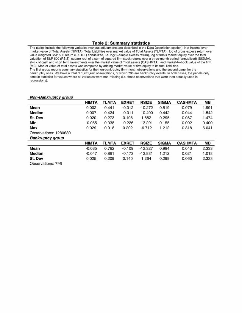
Table 2: Summary statistics The tables include the following variables (various adjustments are described in the Data Description section): Net Income over market value of Total Assets (NIMTA), Total Liabilities over market value of Total Assets (TLMTA), log of gross excess return over value weighted S&P 500 return (EXRET) annualized, i.e. log(1+simple excess return), log of firm�s market equity over the total valuation of S&P 500 (RSIZ), square root of a sum of squared firm stock returns over a three-month period (annualized) (SIGMA), stock of cash and short term investments over the market value of Total assets (CASHMTA), and market-to-book value of the firm (MB). Market value of total assets was computed by adding market value of firm equity to its total liabilities. The first group reports summary statistics for the non-bankruptcy firm-month observations and the second panel for the bankruptcy ones. We have a total of 1,281,426 observations, of which 796 are bankruptcy events. In both cases, the panels only contain statistics for values where all variables were non-missing (i.e. those observations that were then actually used in regressions).

Non-Bankruptcy group NIMTA TLMTA EXRET RSIZE SIGMA CASHMTA MB Mean 0.002 0.441 -0.012 -10.272 0.519 0.079 1.991 Median 0.007 0.424 -0.011 -10.400 0.442 0.044 1.542 St. Dev 0.020 0.273 0.108 1.882 0.295 0.087 1.474 Min -0.055 0.038 -0.226 -13.291 0.155 0.002 0.400 Max 0.029 0.918 0.202 -6.712 1.212 0.318 6.041 Observations: 1280630 Bankruptcy group NIMTA TLMTA EXRET RSIZE SIGMA CASHMTA MB Mean -0.035 0.762 -0.109 -12.327 0.994 0.043 2.333 Median -0.047 0.861 -0.173 -12.881 1.212 0.021 1.018 St. Dev 0.025 0.209 0.140 1.264 0.299 0.060 2.333 Observations: 796

Table 3: Logit regressions of default indicator on predictor variables This table reports results from logit regressions of the default indicator on predictor variables. The value of the predictor variable is known at the beginning of the month over which bankruptcy is measured. Net income and total liabilities are scaled by accounting and market total assets.

(1) (2) (3) (4) (5) (6)

NITA -16.728 (15.47)** NIMTA -33.322 -32.935 (19.62)** (19.91)** NIMTAAVG -42.701 -42.754 -42.768 (19.47)** (19.28)** (19.27)** TLTA 5.612 (25.06)** TLMTA 4.866 4.827 4.706 4.479 4.790 (25.27)** (25.71)** (25.06)** (23.51)** (23.61)** EXRET -3.566 -3.126 -3.111 (11.96)** (10.61)** (10.72)** EXRETAVG -10.993 -11.674 -11.529 (13.40)** (14.16)** (13.95)** SIGMA 2.776 2.777 2.749 2.212 2.060 2.497 (16.16)** (16.29)** (16.29)** (12.74)** (11.88)** (12.39)** RSIZE -0.123 -0.036 -0.043 0.030 0.038 0.029 (3.29)** (0.98) (1.20) (0.84) (1.04) (0.80) CASHMTA -4.954 -4.826 (7.93)** (7.74)** MB 0.124 0.124 (7.73)** (7.76)** DD 0.094 (4.79)** SIGMAMISS 1.272 1.095 1.110 1.165 (6.22)** (5.31)** (5.38)** (5.64)** Constant -15.158 -13.586 -13.611 -12.618 -12.234 -13.160 (36.58)** (34.88)** (35.11)** (32.60)** (31.02)** (29.60)** Observations 1197376 1264108 1281426 1281426 1281426 1281426 No. of bankruptcies 737 762 796 796 796 796 Pseudo R squared 0.268 0.273 0.268 0.282 0.293 0.295 Absolute value of z statistics in parentheses * significant at 5%; ** significant at 1%

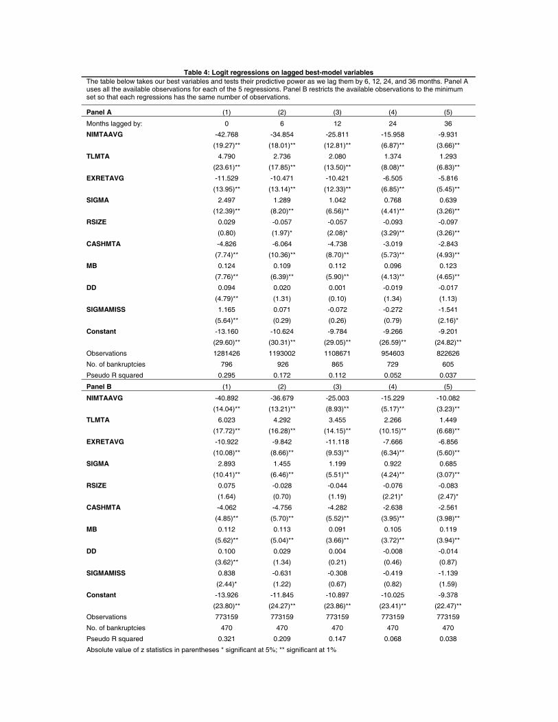
Table 4: Logit regressions on lagged best-model variables The table below takes our best variables and tests their predictive power as we lag them by 6, 12, 24, and 36 months. Panel A uses all the available observations for each of the 5 regressions. Panel B restricts the available observations to the minimum set so that each regressions has the same number of observations.

Panel A (1) (2) (3) (4) (5)

Months lagged by: 0 6 12 24 36

NIMTAAVG -42.768 -34.854 -25.811 -15.958 -9.931

(19.27)** (18.01)** (12.81)** (6.87)** (3.66)**

TLMTA 4.790 2.736 2.080 1.374 1.293

(23.61)** (17.85)** (13.50)** (8.08)** (6.83)**

EXRETAVG -11.529 -10.471 -10.421 -6.505 -5.816

(13.95)** (13.14)** (12.33)** (6.85)** (5.45)**

SIGMA 2.497 1.289 1.042 0.768 0.639

(12.39)** (8.20)** (6.56)** (4.41)** (3.26)**

RSIZE 0.029 -0.057 -0.057 -0.093 -0.097

(0.80) (1.97)* (2.08)* (3.29)** (3.26)**

CASHMTA -4.826 -6.064 -4.738 -3.019 -2.843

(7.74)** (10.36)** (8.70)** (5.73)** (4.93)**

MB 0.124 0.109 0.112 0.096 0.123

(7.76)** (6.39)** (5.90)** (4.13)** (4.65)**

DD 0.094 0.020 0.001 -0.019 -0.017

(4.79)** (1.31) (0.10) (1.34) (1.13)

SIGMAMISS 1.165 0.071 -0.072 -0.272 -1.541

(5.64)** (0.29) (0.26) (0.79) (2.16)*

Constant -13.160 -10.624 -9.784 -9.266 -9.201

(29.60)** (30.31)** (29.05)** (26.59)** (24.82)**

Observations 1281426 1193002 1108671 954603 822626

No. of bankruptcies 796 926 865 729 605

Pseudo R squared 0.295 0.172 0.112 0.052 0.037

Panel B (1) (2) (3) (4) (5)

NIMTAAVG -40.892 -36.679 -25.003 -15.229 -10.082

(14.04)** (13.21)** (8.93)** (5.17)** (3.23)**

TLMTA 6.023 4.292 3.455 2.266 1.449

(17.72)** (16.28)** (14.15)** (10.15)** (6.68)**

EXRETAVG -10.922 -9.842 -11.118 -7.666 -6.856

(10.08)** (8.66)** (9.53)** (6.34)** (5.60)**

SIGMA 2.893 1.455 1.199 0.922 0.685

(10.41)** (6.46)** (5.51)** (4.24)** (3.07)**

RSIZE 0.075 -0.028 -0.044 -0.076 -0.083

(1.64) (0.70) (1.19) (2.21)* (2.47)*

CASHMTA -4.062 -4.756 -4.282 -2.638 -2.561

(4.85)** (5.70)** (5.52)** (3.95)** (3.98)**

MB 0.112 0.113 0.091 0.105 0.119

(5.62)** (5.04)** (3.66)** (3.72)** (3.94)**

DD 0.100 0.029 0.004 -0.008 -0.014

(3.62)** (1.34) (0.21) (0.46) (0.87)

SIGMAMISS 0.838 -0.631 -0.308 -0.419 -1.139

(2.44)* (1.22) (0.67) (0.82) (1.59)

Constant -13.926 -11.845 -10.897 -10.025 -9.378

(23.80)** (24.27)** (23.86)** (23.41)** (22.47)**

Observations 773159 773159 773159 773159 773159

No. of bankruptcies 470 470 470 470 470

Pseudo R squared 0.321 0.209 0.147 0.068 0.038

Absolute value of z statistics in parentheses * significant at 5%; ** significant at 1%

Table 5: Logit regressions with macro variables

The regressions below include two macro variables. Regression in column 1 includes default yield spread (DFY), the spread between the yields on BAA and AAA rated debt. Regression in column two includes term spread (TMS), the difference between yields on a 10-year government bond and 6-month T-Bill. Both regressions include interactions of these two variables with relative size (RSIZE) and leverage (TLMTA).

(1) (2) NIMTAAVG -42.229 -42.407 (18.95)** (19.07)** TLMTA 6.312 5.675 (14.03)** (13.53)** TLMTA*DFY -175.289 (5.09)** TLMTA*TMS -63.873 (3.36)** EXRETAVG -11.454 -11.719 (13.90)** (14.12)** SIGMA 2.184 2.062 (12.72)** (11.87)** RSIZE 0.164 0.048 (2.13)* (0.84) RSIZE*DFY -13.020 (2.25)* RSIZE*TMS -0.252 (0.10) CASHMTA -4.667 -4.893 (7.46)** (7.81)** MB 0.127 0.121 (7.94)** (7.58)** SIGMAMISS 0.971 1.093 (4.72)** (5.30)** DFY 37.025 (0.51) TMS 53.101 (1.60) Constant -12.831 -13.134 (13.80)** (18.18)** Observations 1243098 1243098 No. of bankruptcies 792 792 Pseudo R squared 0.299 0.294 Absolute value of z statistics in parentheses * significant at 5%; ** significant at 1%

Tab

le 6

: E

qu

ity

Ret

urn

s o

n b

ankr

up

tcy

po

rtfo

lios

We

sort

ed a

ll st

ocks

bas

ed o

n th

e pr

edic

ted

prob

abili

ty o

f ban

krup

tcy

13-m

onth

s ah

ead

(a 1

2-m

onth

lag

to o

ur b

asic

mod

el)

and

divi

ded

them

into

10

port

folio

s ba

sed

on

perc

entil

e cu

toffs

. For

exa

mpl

e, 0

to 5

th p

erce

ntile

(00

05)

and

99th

to 1

00th

per

cent

ile (

9900

). In

the

tabl

e be

low

we

show

res

ults

from

reg

ress

ions

on

a co

nsta

nt, e

xces

s m

arke

t re

turn

(R

M),

as

wel

l as

thre

e (R

M, H

ML,

SM

B)

and

four

(R

M, H

ML,

SM

B, U

MD

) F

F fa

ctor

reg

ress

ions

. Pan

el A

sho

ws

alph

as fr

om th

ese

regr

essi

ons

and

the

corr

espo

ndin

g t-

stat

be

low

. Pan

el B

sho

ws

load

ings

on

the

thre

e fa

ctor

s, a

s w

ell a

s co

rres

pond

ing

t-st

ats

belo

w, f

rom

the

3-fa

ctor

reg

ress

ion.

The

last

row

in P

anel

B r

epor

ts m

onth

ly s

tand

ard

devi

atio

n of

the

port

folio

ret

urns

.

Pan

el A

P

ort

folio

s 00

05

0510

10

20

2040

40

60

6080

80

90

9095

95

99

9900

M

ean

retu

rn

0.00

6 0.

004

0.00

3 0.

002

0.00

1 0.

001

0.00

0 -0

.002

-0

.002

-0

.004

(3.7

4)**

(2

.64)

**

(2.1

9)*

(1.4

8)

(0.4

0)

(0.5

5)

(0.0

5)

(0.5

4)

(0.5

7)

(0.6

6)

CA

PM

alp

ha

0.00

6 0.

003

0.00

2 0.

001

0.00

0 0.

001

-0.0

01

-0.0

03

-0.0

03

-0.0

06

(3

.68)

**

(2.2

5)*

(1.4

7)

(0.9

8)

(0.2

9)

(0.5

2)

(0.2

3)

(0.8

2)

(0.7

8)

(0.8

8)

3-fa

ctor

alp

ha

0.00

5 0.

004

0.00

2 0.

001

-0.0

01

-0.0

02

-0.0

04

-0.0

07

-0.0

08

-0.0

13

(6

.28)

**

(4.5

6)**

(4

.11)

**

(1.3

7)

(2.1

5)*

(1.6

8)

(2.7

4)**

(2

.87)

**

(2.5

2)*

(2.0

4)*

4-fa

ctor

alp

ha

0.00

4 0.

003

0.00

1 0.

000

-0.0

01

-0.0

01

-0.0

04

-0.0

06

-0.0

08

-0.0

10

(5

.22)

**

(3.3

7)**

(2

.59)

* (0

.61)

(2

.12)

* (0

.98)

(2

.41)

* (2

.46)

* (2

.25)

* (1

.52)

Pan

el B

P

ort

folio

s 00

05

0510

10

20

2040

40

60

6080

80

90

9095

95

99

9900

R

M

-0.1

29

-0.0

95

-0.0

35

-0.0

32

-0.0

46

-0.0

34

0.03

4 0.

052

0.05

9 0.

204

(6

.27)

**

(4.8

9)**

(2

.71)

**

(2.6

0)**

(3

.31)

**

(1.4

7)

(0.9

3)

(0.9

0)

(0.7

1)

(1.3

0)

HM

L 0.

014

-0.1

36

-0.1

39

0.02

7 0.

222

0.38

4 0.

527

0.59

2 0.

766

1.08

7

(0.4

3)

(4.2

5)**

(6

.52)

**

(1.3

6)

(9.7

8)**

(1

0.02

)**

(8.8

0)**

(6

.30)

**

(5.6

9)**

(4

.24)

**

SM

B

0.85

3 0.

786

0.70

5 0.

741

0.82

1 0.

957

1.29

9 1.

509

1.76

7 1.

944

(2

7.43

)**

(26.

60)*

* (3

5.76

)**

(40.

34)*

* (3

9.06

)**

(26.

95)*

* (2

3.42

)**

(17.

29)*

* (1

4.16

)**

(8.1

7)**

S

t. D

evia

tion

0.02

5 0.

024

0.02

1 0.

020

0.02

3 0.

029

0.04

1 0.

054

0.07

0 0.

112

Bankruptcy percentage per year (1963-1998)

0.00

0.20

0.40

0.60

0.80

1.00

1.20

1.40

1.60

1.80

2.00

1963 1964 1965 1966 1967 1968 1969 1970 1971 1972 1973 1974 1975 1976 1977 1978 1979 1980 1981 1982 1983 1984 1985 1986 1987 1988 1989 1990 1991 1992 1993 1994 1995 1996 1997 1998

(%)

Figure 1 The graph shows the percentage of active firms (where the number of firms in a year is taken as the average over the year) that were bankrupt in any given year over the period 1963-1998.

050

-.05 0 .05

NI/MTA in the bankruptcy firm-month

Per

cent

NI_MTA_qGraphs by Default

02

46

-.06 -.04 -.02 0 .02

NI/MTA in the non-bankruptcy firm-month

Per

cent

NI_MTA_qGraphs by Default

NI / MTA for bankruptcy and non - bankruptcy firm - months

Figure 2 The graph above shows the distribution of the company�s Net Income over market-adjusted Total Assets (the sum of market value of equity and book value of Total Liabilities) for the firm-month when the firm was in bankruptcy (left) and all others (right). The mass points in either graph represent the effect of winsorization (i.e. the resulting mass points). The variable has also been lagged to ensure that the information was the latest publicly available in the month with which it is associated.

010

2030

40

0 .5 1

TL/MTA in the bankruptcy firm-month

Per

cent

TL_MTA_qGraphs by Default

02

46

8

0 .5 1

TL/MTA in the non-bankruptcy firm-month

Per

cent

TL_MTA_qGraphs by Default

TL / MTA for bankruptcy and non - bankruptcy firm - months

Figure 3 The graph above shows the distribution of the company�s Total Liabilities over market-adjusted Total Assets (the sum of market value of equity and book value of Total Liabilities) for the firm-month when the firm was in bankruptcy (left) and all others (right). The mass points in either graph represent the effect of winsorization (i.e. the resulting mass points). The variable has also been lagged to ensure that the information was the latest publicly available in the month with which it is associated.

010

2030

40

-4 -2 0 2

EXRET in the bankruptcy firm-month

Per

cent

EXRET_annGraphs by Default

02

46

-2 0 2 4

EXRET in the non-bankruptcy firm-month

Per

cent

EXRET_annGraphs by Default

EXRET for bankruptcy and non - bankruptcy firm - months

Figure 4 The graph above shows the distribution of the log gross excess monthly return on company stock over the value-weighted S&P500 Index (EXRET) for the firm-month when the firm was in bankruptcy (left) and all others (right). It was constructed as the log of a gross return based on the simple difference between the return on the company stock and return on the index in a given month. The mass points in either graph represent the effect of winsorization (i.e. the resulting mass points). The variable has also been lagged to ensure that the information was the latest publicly available in the month with which it is associated.

050

-14 -12 -10 -8 -6

RSIZ in the bankruptcy firm-month

Per

cent

RSIZGraphs by Default

02

46

-14 -12 -10 -8 -6

RSIZ in the non-bankruptcy firm-month

Per

cent

RSIZGraphs by Default

RSIZ for bankruptcy and non - bankruptcy firm - months

Figure 5 The graph above shows the distribution of the log of the ratio of company�s market equity and S&P 500 index total market valuation (RSIZ) for the firm-month when the firm was in bankruptcy (left) and all others (right). The mass points in either graph represent the effect of winsorization (i.e. the resulting mass points). The variable has also been lagged to ensure that the information was the latest publicly available in the month with which it is associated.

020

4060

0 .5 1 1.5

SIGMA in the bankruptcy firm-month

Per

cent

SIGMAGraphs by Default

02

46

0 .5 1 1.5

SIGMA in the non-bankruptcy firm-month

Per

cent

SIGMAGraphs by Default

SIGMA for bankruptcy and non - bankruptcy firm - months

Figure 6 The graph above shows the distribution of the estimate of daily return variations (annualized) -- constructed by summing over squared daily returns in any given month and diving by the number of observations less 1 -- for the firm-month when the firm was in bankruptcy (left) and all others (right). The mass points in either graph represent the effect of winsorization (i.e. the resulting mass points). The variable has also been lagged to ensure that the information was the latest publicly available in the month with which it is associated.

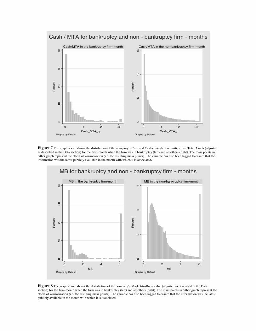
010

2030

40

0 .1 .2 .3

Cash/MTA in the bankruptcy firm-month

Per

cent

Cash_MTA_qGraphs by Default

05

1015

0 .1 .2 .3

Cash/MTA in the non-bankruptcy firm-month

Per

cent

Cash_MTA_qGraphs by Default

Cash / MTA for bankruptcy and non - bankruptcy firm - months

Figure 7 The graph above shows the distribution of the company�s Cash and Cash equivalent securities over Total Assets (adjusted as described in the Data section) for the firm-month when the firm was in bankruptcy (left) and all others (right). The mass points in either graph represent the effect of winsorization (i.e. the resulting mass points). The variable has also been lagged to ensure that the information was the latest publicly available in the month with which it is associated.

010

2030

40

0 2 4 6

MB in the bankruptcy firm-month

Per

cent

MBGraphs by Default

02

46

0 2 4 6

MB in the non-bankruptcy firm-month

Per

cent

MBGraphs by Default

MB for bankruptcy and non - bankruptcy firm - months

Figure 8 The graph above shows the distribution of the company�s Market-to-Book value (adjusted as described in the Data section) for the firm-month when the firm was in bankruptcy (left) and all others (right). The mass points in either graph represent the effect of winsorization (i.e. the resulting mass points). The variable has also been lagged to ensure that the information was the latest publicly available in the month with which it is associated.

Predicted vs. Actual Bankruptcies (annual)

0.00%

0.20%

0.40%

0.60%

0.80%

1.00%

1.20%

1.40%

1.60%

1.80%

2.00%

1963

1965

1967

1969

1971

1973

1975

1977

1979

1981

1983

1985

1987

1989

1991

1993

1995

1997

Actual

Predicted

Figure 9 The graph above represents the percentage of aggregate bankruptcies as predicted by our model and the actual bankruptcies that occurred in that year. To get the predicted percentage of bankruptcies, we average over the predicted probability (based on our model) of all active firms in a given month.

Coefficients on year dummies (no regressors)

-1

-0.8

-0.6

-0.4

-0.2

0

0.2

0.4

0.6

0.8

1

1976 1977 1978 1979 1980 1981 1982 1983 1984 1985 1986 1987 1988 1989 1990 1991 1992 1993 1994 1995 1996 1997 1998

Figure 10 The graph above shows the deviation of the year dummy coefficients from their sample mean. The coefficient estimates are from the regression that included only dummies. The number of observations is equal to that in our best model regression. The dotted line shows a 2 standard deviation confidence interval around zero for each coefficient value.

Coefficients on year dummies (best model)

-1

-0.8

-0.6

-0.4

-0.2

0

0.2

0.4

0.6

0.8

1

1976 1977 1978 1979 1980 1981 1982 1983 1984 1985 1986 1987 1988 1989 1990 1991 1992 1993 1994 1995 1996 1997 1998

Figure 11 The graph above shows the deviation of the year dummy coefficients from their sample mean. The coefficient

estimates are from our best fitting regression. The dotted line shows a 2 standard deviation confidence interval around zero for each coefficient value.

Loadings on FF factors

-0.15

-0.1

-0.05

0

0.05

0.1

0.15

0.2

0.25

0005 0510 1020 2040 4060 6080 8090 9095 9599 9900

-0.5

0

0.5

1

1.5

2

2.5

RM

HML

SMB

Figure 12 The graph above shows the loadings (betas) on Fama-French factors from the regressions of bankruptcy portfolios on the three factors (RM, HML, SMB).

Alphas for bankruptcy portfolios

-0.015

-0.01

-0.005

0

0.005

0.01

0005 0510 1020 2040 4060 6080 8090 9095 9599 9900

FF alpha

CAPM alpha

Mean return

Figure 13 The graph shows alphas from various regressions: regression on a constant (Mean return), three-factor regression (FF alpha) and the CAPM regression (CAPM alpha).