in school and out of trouble? the minimum dropout age and...

1

In School and Out of Trouble? The Minimum Dropout Age and Juvenile Crime

D. Mark Anderson

Department of Agricultural Economics and Economics

Montana State University

[email protected]

September 2012

Abstract

Does increasing the minimum dropout age reduce juvenile crime rates? Despite

popular accounts that link school attendance to keeping youth out of trouble, little

systematic research has analyzed the contemporaneous relationship between

schooling and juvenile crime. This paper examines the connection between the

minimum age at which youth can legally drop out of high school and juvenile

arrest rates by exploiting state-level variation in the minimum dropout age. Using

county-level arrest data for the United States between 1980 and 2008, a

difference-in-difference-in-difference-type empirical strategy compares the arrest

behavior over time of various age groups within counties that differ by their

state’s minimum dropout age. The evidence suggests that minimum dropout age

requirements have a significant and negative effect on property and violent crime

arrest rates for individuals aged 16 to 18 years-old, and these estimates are robust

to a range of specification checks. While other mechanisms cannot necessarily be

ruled out, the results are consistent with an incapacitation effect; school

attendance decreases the time available for criminal activity.

Keywords: Minimum dropout age; Juvenile crime; Delinquency

JEL classification: H75; I20; I28; K42

I owe thanks to Dean Anderson, Yoram Barzel, Shawn Bushway, Rachel Dunifon, Andy Hanssen, Wolf Latsch,

Lars Lefgren, Lance Lochner, Jens Ludwig, Shelly Lundberg, Claus Pörtner, Randy Rucker, Alan Seals, Lan Shi,

Wendy Stock, Chris Stoddard, Mary Beth Walker and seminar participants at Montana State University, the

University of Washington, the 2009 Southern Economic Association’s annual meeting, and the 2010 Population

Association of America’s annual meeting for comments and suggestions. I also owe a special thanks to Philip

Oreopoulos for providing data on minimum dropout age laws, Thomas Dee for providing data on minimum legal

drinking ages, and Lisa Whittle for help with obtaining the YRBS data. All errors and omissions in this paper are

solely mine.

mailto:[email protected]

2

“Dropout prevention is crime prevention.”

Lee Baca, Los Angeles County Sheriff

I. Introduction

Does increasing the minimum age at which youth are legally permitted to leave school

keep them off the streets and away from crime? Previous research illustrates a correlation

between youth dropouts and juvenile criminal behavior (see, e.g., Thornberry et al. 1985; Fagan

and Pabon 1990). In the state of California alone, dropouts are estimated to be responsible for

1.1 billion dollars in annual juvenile crime costs.1 Because of crime’s deleterious consequences,

it is important to understand whether or not being in school has a causal influence on juvenile

offending; evidence suggests that involvement in juvenile crime adversely impacts economic

outcomes later in life. Incarceration during adolescence is associated with lower educational

attainment and decreased future earnings (Waldfogel 1994a; Waldfogel 1994b; Hjalmarsson

2008). Furthermore, juvenile crime not only has an immediate impact on the delinquent and

their victim(s), but can impose negative externalities on those not directly involved with criminal

acts (see, e.g., Grogger 1997).

Previous studies have focused on a wide array of determinants of juvenile crime. In

general, much of the literature has concentrated on deterrence and punishment as crime-reducing

mechanisms.2 Research has also documented the impact of wages (Grogger 1998), high school

experience (Arum and Beattie 1999), youth employment (Apel et al. 2008), underage drinking

(French and Maclean 2006), and curfew ordinances (Kline 2009) to name a few.

1 This number reflects an estimate that includes criminal justice expenditures, incarceration costs, school disruption

costs and victim costs (Belfield and Levin 2009). 2 See, for example, Becker (1968), Freeman (1996), Levitt (1998), and Corman and Mocan (2000).

3

This paper joins the sparse, yet growing, literature on the effects of education on crime by

investigating the relationship between the minimum dropout age (MDA) and juvenile arrest

rates.3 In general, the literature can be divided into two categories: the longer-run relationship

between education and crime and the contemporaneous relationship between education and

crime. Research on the longer-run has focused on the impact of educational attainment on

subsequent criminal behavior. More specifically, these studies are interested in whether the

accumulation of education as a youth has an impact on adult criminality. Empirical research in

this area is not decisive. Tauchen et al. (1994) and Witte and Tauchen (1994) find that having a

parochial school education is associated with lower criminal behavior, but a high school degree

has no effect. Grogger’s (1998) results indicate that wages have a negative effect on crime, but

having additional years of education or a high school diploma do not influence criminal activity.

However, Grogger’s (1998) findings do not rule out education having an indirect impact on

crime through the labor market. On the other hand, Lochner (2004), Lochner and Moretti

(2004), and Buonanno and Leonida (2009) illustrate that education is negatively related to adult

crime. In a similar vein, Deming’s (2011) results suggest that school quality predicts subsequent

criminal behavior.

To date, considerably fewer studies have investigated the contemporaneous relationship

between schooling and crime. This paper fits within this area of research. Gottfredson (1985),

Farrington et al. (1986), and Witte and Tauchen (1994) find that time spent at school is

associated with lower levels of criminal behavior. These studies do not control, however, for the

potential endogeneity of schooling. Jacob and Lefgren (2003) and Luallen (2006) estimate the

impact of school attendance on crime by exploiting variation in teacher in-service days and

3 For a more comprehensive review of the literature, see the excellent discussion by Lochner (2010).

4

teacher strike days, respectively. Both papers show that property crimes committed by juveniles

decrease when school is in session, but violent juvenile crime rates increase on these days. The

authors suggest that incapacitation effects likely explain the property crime results, while

concentration effects may underlie the violent crime findings. An incapacitation effect of school

is that it keeps juveniles occupied, leaving less time and opportunity to commit crimes. In

contrast, keeping children in school increases the number of potential interactions that facilitate

delinquency, especially physical altercations.

This paper exploits the spatial and temporal variation in minimum dropout age laws to

find strong evidence that increases in the minimum dropout age reduce rates of property and

violent crime among high school-aged individuals. Estimates for drug-related crimes are large in

magnitude and negative in sign, but are generally not statistically significant. Though this paper

presents robust evidence on the effect of MDA laws on property and violent crime arrest rates, it

is not possible to precisely pin down the channels through which education impacts crime.

Nevertheless, by studying effects across age groups and types of crimes, it is possible to provide

suggestive evidence on the mechanisms that are relatively important. Specifically, the results are

consistent with an incapacitation effect; however, it should be noted that other mechanisms

cannot necessarily be ruled out (e.g. human capital effects). These findings suggest that policies

designed to keep kids in school may be successful at decreasing delinquent behavior.

This paper makes at least four important contributions to the literature. First, previous

research has not systematically analyzed the effects of minimum dropout age laws on juvenile

crime. Second, Jacob and Lefgren (2003) and Luallen (2006) are only able to test for the

existence of extremely short-run effects of school attendance. An increase in the minimum

dropout age can result in students staying in school for up to two additional years. In-service and

5

strike days consist of much shorter lengths of time. Consequently, the school attendance and

crime dynamic is likely to differ considerably between these policies.

Third, by explicitly examining changes in MDA laws, this paper's focus is on the

marginal juvenile who is legally obligated to stay in school longer. While Jacob and Lefgren

(2003) and Luallen (2006) analyze mechanisms that release entire student bodies from school,

this paper concentrates on a policy that affects a small portion of the high school-aged

population. Arguably, students on the margin of dropping out are of the utmost importance from

a policy and social perspective because they represent a group of high risk offenders.

Lastly, after establishing a strong and negative relationship between the MDA and

juvenile crime, this paper discusses the potential for delinquency and other risky behaviors to be

displaced from the streets to schools when the MDA is higher. Using the national Youth Risk

Behavior Survey data, a brief analysis highlights that this is a potentially important issue that

policy-makers should consider when deciding whether or not to increase their state’s minimum

dropout age.

II. Background and relevant literature

In 1852, Massachusetts was the first state to enact a compulsory schooling law. By 1918,

all states had some form of a compulsory schooling law in place (Lleras-Muney 2002). In

general, these laws specify a minimum and maximum age for which attendance is required.

Historically, compulsory schooling laws have changed frequently. Table 1 illustrates there has

been a strong movement towards increasing the minimum dropout age in recent years.4

4 For example, Illinois and Indiana have recently increased their MDA from 16 to 17 and 16 to 18, respectively.

Other states, however, have maintained a constant MDA over the past 50 years. Iowa, Michigan, and Montana have

6

[Table 1 about here.]

Not surprisingly, the legislation is more complex than simply specifying a minimum

dropout age. Some states allow exemptions if the child is working or has obtained parental

consent. States also vary by their punishment of truancy; it is not unusual for a state to punish

the parents of a truant child.5

Previous work has generally focused on compulsory schooling laws to estimate the

returns to education.6 Mentioned above, Lochner and Moretti (2004) estimate the effect of

educational attainment on adult criminal activity using variation in state compulsory schooling

laws to instrument endogenous schooling decisions.7 Other applications of compulsory

schooling include mortality and teenage childbearing (Lleras-Muney 2005; Black et al. 2008).

This study is concerned with the reduced form relationship between the minimum

dropout age and juvenile crime. Implicit to this relationship is that these laws are effective at

impacting attendance rates. Perhaps the most seminal work on this relationship is by Angrist and

Krueger (1991); they find that approximately 25 percent of potential dropouts in the United

States remain in school because of compulsory schooling laws. Results from other research on

the effectiveness of compulsory schooling are consistent with the conclusions drawn from

had a dropout age of 16 during this period, while Ohio, Oklahoma, and Utah have maintained a dropout age of 18.

In addition, several states have raised and lowered their MDA during this time. 5 Oreopoulos (2009) offers a more complete discussion of the legislation. In particular, Table 1 in Oreopoulos

(2009) lists examples of exemptions and punishments for states with a minimum dropout age greater than 16. 6 See, for example, Acemoglu and Angrist (2001) and Oreopoulos (2006a, 2006b).

7 It is important to note that Lochner and Moretti (2004) focus on the number of years of mandatory schooling as

opposed to the minimum dropout age. Though positively correlated, a higher minimum dropout age does not

necessarily mean more years of compulsory schooling because states also differ in their mandatory starting age. For

example, Oregon and Maryland both require 12 years of compulsory schooling; yet, the minimum dropout ages for

Oregon and Maryland are 18 and 16, respectively. Because this paper's attention is on the contemporaneous

relationship between being in school and crime, the minimum dropout age is the variable of interest.

7

Angrist and Krueger (1991).8 Despite the existing evidence, this paper presents results on the

relationship between the minimum dropout age and dropout status. These results, based on U.S.

Census data, are discussed in the Appendix and are presented in Table A1. In short, the results

confirm that increases in the MDA significantly decrease the likelihood of dropping out.

As pointed out by Angrist and Krueger (1991), the efficacy of compulsory schooling

legislation is likely due to two enforcement mechanisms. In a majority of states, children are not

permitted to work during school hours unless they are of an age at or above their state’s

compulsory schooling requirement. Additionally, young workers are required to obtain work

permits that are often granted by school administrators. This, to an extent, allows schools to

monitor the behavior of youth who are below the minimum dropout age. It is possible that

dropouts who seek employment are less likely to commit crimes than those who leave school and

have no interest in working. For the latter individuals, direct enforcement and policing may be

more effective means of mandating attendance. More specifically, state legislation provides

truancy officers to enforce the law; officers are given the authority to arrest truant youth without

a warrant. Truancy regulations are also enforced by school officials and often implemented

under the context of parental responsibility.

III. Data for county-level panel regressions

Dependent variables

8 Li (2006) uses data from the High School and Beyond Survey to show that increasing the dropout age to 18

increases the probability of completing high school. Moreover, he shows the effects are much more pronounced for

disadvantaged students. Wenger (2002) illustrates that increasing a state’s dropout age is consistently predicted to

decrease the probability that an individual will drop out of high school. More specifically, she finds the change in

probability is equivalent to a decrease in the dropout rate of roughly 16 percent. The results in Oreopoulos (2009)

also suggest that more restrictive compulsory schooling laws reduce dropout rates. Using less recent data, Lleras-

Muney (2002) provides strong evidence that compulsory schooling laws were responsible for increased attendance

during the period 1915 to 1939.

8

The juvenile arrest data come from the FBI’s Uniform Crime Reports (UCR).9 These

data are aggregated by the age of the offender at the county-level for the period 1980 to 2008.

Arrest rates are arrests per 1,000 of the specified age group population.10

Arrests are reported for

violent crimes (murder, rape, robbery, aggravated assault, and simple assault), property crimes

(larceny, burglary, motor vehicle theft, and arson) and drug-related crimes (selling and

possession).11

The violent, property, and drug crime indices represent unweighted aggregations

of their respective individual components. While this paper analyzes arrest rates for both sexes,

the majority of the results focus on males because the male arrest rate is roughly four times

higher than the female arrest rate.

Collection of the arrest data was completed through a cooperative effort of self-reporting

by more than 16,000 city, county, and state law enforcement agencies. Of course, with a project

of this magnitude, there are reasons to be cautious of the self-reported data. Gould et al. (2002)

point out that arrest rates understate the true level of crime because not every crime committed is

reported to the police. Moreover, underreporting can vary by crime type or county of

jurisdiction. Data collection and reporting methods may vary by jurisdiction as well.

Fortunately, county fixed effects eliminate the impact of time-invariant, cross-county differences

in data collection and reporting techniques.

9 U.S. Department of Justice, FBI, Uniform Crime Reports: Arrests by Age, Sex, and Race. Washington, DC: U.S.

Department of Justice, FBI; Ann Arbor, MI: Inter-university Consortium for Political and Social Research (ICPSR,

distributor). 10

These rates are calculated using the National Cancer Institute, Surveillance Epidemiology and End Results, U.S.

Population Data. 11

It should be pointed out that “simple assaults” are actually referred to as “other assaults” in the UCR data

codebook. However, because sexual and domestic offenses are given their own code, it is assumed that “other

assaults” are mostly “simple assaults.” This is likely a safe assumption given the age groups of interest.

9

The primary reason for using arrest rates is that detailed age data are not available in the

UCR offense reports.12

Although arrests are not a perfect measure of youth criminal behavior

and understate the true level of crime, other research indicates that arrest data serve as an

accurate representation of underlying criminal activity.13

Furthermore, this type of measurement

error is unlikely correlated with the minimum dropout age.14

Using the UCR data, Lochner and

Moretti (2004) report the correlations between arrests and crimes committed to be very high.15

In choosing the appropriate sample, counties with 10 or fewer years of arrest data

reported are excluded from the analysis. In addition, age-specific county-year arrest counts that

are greater than two standard deviations from the mean for the 29 year period are dropped from

the sample. This is done because each county arrest count is an aggregation of police agency

reports and not all agencies report every year. To further guard against this issue, this paper

controls for the number of agencies reporting within a county for any given year.16

Results from

model specifications without these restrictions are presented in the sensitivity analysis below.

Independent variables

The state minimum dropout ages come from Oreopoulos (2009), the National Center for

Education Statistics’ Digest of Education Statistics, and various reports and policy briefs.

Annual county-level demographic variables come from the U.S. Census Bureau. The regressions

12

It would not be possible to include complete age data in the UCR offense reports because the ages of criminals

who are not caught remain unknown. 13

See, for example, Hindelang (1978, 1981). 14

One worry is that a county might underreport arrests to suggest the MDA is bringing added benefits to the

population. A benefit of the DDD approach is this issue is potentially addressed by differencing arrest rates across

age groups. However, this concern is only quelled if a county underreports for both the 13 to 15 and 16 to 18 year-

old age groups. If a county's underreporting specifically targets the 16 to 18 year-old population, then this remains a

possible problem. The author would like to thank an anonymous referee for bringing this issue up. 15

Lochner and Moretti (2004) report the following correlations: 0.96 for rape and robbery, 0.94 for murder, assault,

and burglary, and 0.93 for auto theft. 16

Following Gould et al. (2002), regressions were also considered where the sample was restricted to counties with

an average population exceeding 25,000 between 1980 and 2008. This selection criterion is intended to capture a

representative population and eliminate counties where arrest reports are more likely to be inaccurate. The results

are similar when the sample is limited in this manner and are available upon request.

10

control for population density, the percentage black, the percentage male, and the percentages in

the age ranges 13 to 15 and 16 to 18. Data on per capita personal income and the annual

prevailing minimum wage are also included and come from the Bureau of Economic Analysis.

These variables are deflated by the Consumer Price Index to convert to 2000 dollars. Data on

each state’s minimum legal drinking age come from Dee (2001). Table 2 presents descriptive

statistics for all counties in the sample.


IV. Empirical strategy

The empirical analysis is reduced form, based on the approach taken by a long line of

researchers to evaluate the effects of county- and state-level variables on aggregate measures of

crime.17

As stated above, this study aims to evaluate the impact of the minimum dropout age on

juvenile arrest rates by exploiting variation in state laws. The question that follows: Are

students who would have otherwise dropped out less likely to commit crimes when forced to stay

in school?

To estimate the impact of the minimum dropout age on juvenile arrest rates, this paper

uses a difference-in-difference-in-difference-type (DDD) empirical strategy.18

This approach

relies on state-wide variation in compulsory schooling laws and on arrest data among age groups

that are plausibly unaffected by the minimum dropout age as controls for unobserved state- and

year-specific juvenile arrest shocks. The control group consists of individuals who are always

17

For examples, see Ludwig (1998) on the effects of concealed-gun-carrying laws on crime; Levitt and Donahue

(2001) and Joyce (2009) on the effects of abortion rates on crime; Grinols and Mustard (2006) on the effects of

casinos on crime; Carpenter (2008) on the effects of underage drunk driving laws on crime; Mocan and Bali (2010)

on the effects of unemployment on crime. 18

Given the availability (or lack thereof) of yearly county-level high school dropout data, a two-stage estimation

strategy was not possible.

11

below the minimum dropout age. Because all states have a minimum dropout age of at least 16,

the control group is comprised of 13 to 15 year-olds.19

The treatment group consists of youth

who are subject to changes in the law (i.e. 16 to 18 year-olds).

The empirical framework relies on the assumption that criminal behavior among

individuals who are below the minimum dropout age tracks the trend of those individuals aged

16 to 18 except that they are not subject to more or less restrictive dropout laws. By utilizing the

control group, common confounding factors are subtracted out from the estimates and the effects

of the policy are more precisely measured. The reference counties chosen for analysis are all

counties in states with a minimum dropout age less than 18. In sum, this strategy compares the

outcomes of youth who are affected by the minimum dropout age to the outcomes of youth who

are not affected by the minimum dropout age (one “difference”) in states with a minimum

dropout age of 16 or 17 versus states with a minimum dropout age of 18 (a second “difference”)

over time (the third “difference”). This paper estimates the following equation:

ArrestRateijst = α + β1MDA18st + β2age16to18i + β3(MDA18st * age16to18i) (1)

+ Xjstβ4 + Cj β5 + Tt β6 + Trends β7 + εijst,

where i indexes the age group, j indexes the county, s indexes the state, and t indexes the year.20

In equation (1), the dependent variable ArrestRate denotes the arrest rate per 1,000 of age

group i in county j and state s at time t. On the right-hand side, MDA18 is equal to one if the

19

The one exception is Mississippi. From 1980 to 1993, Mississippi had a minimum dropout age of 14. The results

are robust when Mississippi counties are excluded from the analysis. 20

In a previous version of this paper, an indicator and interaction terms for MDA17 were also included on the right-

hand-side of (1). Counties in MDA = 17 states are considered reference counties (along with counties in MDA = 16

states) in this version for the sake of brevity when discussing the results. More importantly, the trend among states

has been to increase their MDA to 18. This paper highlights that point by focusing solely on indicators for MDA =

18 counties and provides results that are clearly interpretable in the context of the current policy environment.

Results that include the MDA17 variables are available upon request.

12

state has a minimum dropout age of 18 at time t, and is equal to zero otherwise. The variable

age16to18 is a dummy that controls for differences between 16 to 18 year-olds and 13 to 15

year-olds that are common across years. The variable X is a vector containing the county- and

state-level controls described above. The variables C and T represent county fixed effects and

year effects, respectively. The county fixed effects control for differences in counties that are

common across years, while the year effects control for differences across time that are common

to all counties and to individuals of all ages. Lastly, the variable Trend represents a vector of

linear state-specific time trends that account for time-series variation within each state. In the

Appendix, Table A2 shows results where equation (1) is altered to allow for differential

treatment effects for 16, 17, and 18 year-olds.

The coefficient of interest is β3. This interaction term coefficient represents the marginal

effect of the policy on the treatment group relative to the control group. If increases in the MDA

decrease crime among juveniles 16 to 18 years of age, then we expect β3 to be negative.

This estimation approach addresses at least three important endogeneity problems. First,

there is a strong association between age and crime rates. As a result, comparing the criminal

behavior of 16-18 year-olds to 13-15 year-olds raises some concerns. This method, however,

alleviates this issue because it also compares arrest rates of 16-18 year-olds in states with a

minimum dropout age of 18 to arrest rates of 16-18 year-olds in states with a dropout age of 16

or 17. Second, expectations of when a student will be able to drop out may influence current

criminal behavior. For example, a 16 year-old in a state with a minimum dropout age of 17 may

behave differently than a 16 year-old in a state with a minimum dropout age of 18 because the

former anticipates being able to drop out sooner. Again, this approach mitigates these concerns

because it compares individuals of different ages within states that have similar minimum

13

dropout ages. Lastly, this technique controls for the potential endogeneity of the minimum

dropout age laws. This is accomplished by differencing over time. That is, changes in arrest

rates are examined as opposed to differences in levels. As a result, permanent differences in the

characteristics of states are taken into account.

All models are estimated with weighted least squares where mean county populations are

used as weights. Following Bertrand et al. (2004), standard errors are corrected for clustering at

the state level. This procedure accounts for the possibility that standard errors may be biased due

to serial correlation of the policy variable over time within a state.

A caveat to mention is that the classification of states with respect to MDA laws is basic.

The approach merely relies on the presence of a law in a state during a specific year and does not

control for particular nuances in the laws. As noted previously, state laws vary along several

dimensions, but a practical, parsimonious way to empirically consider all the differences is not

clear. Besides an attempt made below to address major MDA exemptions, the empirical strategy

simply estimates the average effects of these laws and the differences in outcomes across states

by the general classification of each state’s dropout age.

V. Results

Tables 3a and 3b provide a breakdown of the mean arrest rates by age group and the

prevailing MDA law for males and females, respectively. It is immediately apparent the two age

groups display different levels of criminal behavior. Fortunately, the empirical strategy relies

only on the assumption that the rates of crime between the two groups trend with each other over

14

time. Interestingly, for many crimes, the mean rate of arrest is highest in MDA = 18 counties.21

However, it is imperative to note these are only simple means and a more rigorous approach is

required to address causality. The means are calculated such that a county in a state that changes

its MDA is recorded under both dropout age regimes. For example, if a county is in a state that

changes from an MDA = 16 to an MDA = 18, the mean rates of arrest are classified under an

MDA = 16 before the policy change and under an MDA = 18 after the policy change.

[Table 3a about here.]

[Table 3b about here.]

Before discussing the results based on estimation of equation (1), it is useful to consider a

more explicit test for whether changes in criminal behavior take place after MDA laws change.

Figure 1 presents point estimates (with 95 percent confidence intervals) from a simple regression

designed to capture intertemporal effects.22

Two lead dummies, five lag dummies, and an

indicator for the year a state law changed are considered as independent variables in a regression

that also includes county and year fixed effects.23

The dependent variable is the arrest rate for 16

to 18 year-old males for all crimes (i.e. property + violent + drug crimes). The coefficient

estimates for the lead dummies shown in Figure 1 strongly suggest that states that increase their

MDA do not have different arrest rates for 16 to 18 year-olds during the two years prior to a

policy change. However, all lag dummies have coefficient estimates that are negative and

relatively large in magnitude.24

This indicates that arrest rates among the population of interest

21

Arson is the only crime where 13 to 15 year-olds appear to participate at higher rates than 16 to 18 year-olds for

both males and females. 22

Grinols and Mustard (2006) use this approach to analyze the effects of casinos on crime. 23

For example, the first of the two lead dummies takes on a value of one two years prior to a law change in a

particular state, and is equal to zero otherwise. This variable is always equal to zero for counties in states that do not

change their MDA during the sample time frame. 24

The coefficient estimates (with p-values for the t-statistics) for the lags are as follows: lag 1 = -2.10 (p-value =

0.27); lag 2 = -3.34 (p-value = 0.16); lag 3 = -5.20 (p-value = 0.05); lag 4 = -3.21 (p-value = 0.14); lag 5 = -5.50 (p-

15

have fallen after increases in the MDA and motivates proceeding forward with a more careful

empirical approach. In particular, this method does not account for important outside factors that

may have occurred alongside MDA increases that also influenced arrest rates.25

[Figure 1 about here.]

Table 4 presents estimates for β3 from equation (1) where each cell illustrates results from

a separate regression. For males, the estimates are negative in sign and large in magnitude across

all model specifications. With the exception of drug-related arrests, all estimates are statistically

significant at the 10 percent level or better.26

Though not reported for the sake of brevity, it is

worth noting that β1 from equation (1) is not statistically significant for any of the specifications

for males in Table 4. This implies that 13 to 15 year-old males in MDA = 18 states do not have

statistically significantly different arrest rates than males of the same age in MDA = 16 or MDA

= 17 states. The results in the bottom panel of Table 4 illustrate a negative but statistically

insignificant relationship between the MDA and the overall arrest rate among females.

However, it does appear that a higher MDA reduces the rate of violent female offending.


The estimate from the full specification for males in Column 3 of Table 4 indicates that

exposure to an MDA = 18 reduces the overall arrest rate for 16 to 18 year-olds by 10.27

incidences per 1,000 of the age group population. To put this estimate into perspective, this

represents a 17.2 percent decrease from the mean arrest rate for 16 to 18 year-olds in states with

value = 0.01). For example, the estimated coefficient of lag 5 indicates that the arrest rate was lower by 5.5 arrests

per 1,000 of the 16 to 18 year-old population five years after an increase in the MDA. 25

When this approach is applied to 13 to 15 year-old male arrest rates, the “control” rates, there is no evidence of a

relatively discrete and persistent drop following MDA increases. This provides further confidence that the results in

Figure 1 are illustrating a causal effect of changes in the dropout age. 26

Because the county fixed effects explain most of the variation in crime, models without these were also

considered in an even more basic specification. For males, the coefficient estimates remained negative and similar

in magnitude to the results shown in Table 4.

16

an MDA = 16 or an MDA = 17. For male property crime arrests, an MDA = 18 is associated

with a 9.9 percent reduction from the mean arrest rate for 16 to 18 year-olds in states with an

MDA = 16 or an MDA = 17. For male violent crime arrests, an MDA = 18 is associated with a

22.5 percent reduction from the mean arrest rate for 16 to 18 year-olds in states with an MDA =

16 or an MDA = 17.

Because this paper relies on a reduced form approach, it is important to consider whether

the magnitudes of these effects are plausible. The Census analysis in the Appendix indicates that

a one year increase in the MDA is associated with roughly a 2 percentage point decrease in the

dropout rate. According to the U.S. Department of Education, the status high school completion

rate was nearly 90 percent in 2009 (Chapman et al. 2011). This implies that roughly 20 percent

of those who drop out would stay in school with a one year increase in the MDA. Given that

over 1.2 million youths drop out annually, this would mean that approximately 240,000 more

students per year would stay in school with a higher MDA (Alliance for Excellent Education

2007).27

Using property crimes as an example, the UCR data indicate that 16 to 18 year-old

males were responsible for roughly 175,000 arrests in 2008. A decrease of 9.9 percent means

that over 17,000 fewer property crimes are committed annually when the dropout age is higher.

Taken together, these figures imply that for every 100 students kept from dropping out there

would be over 7 fewer property crimes committed. Although these are simple back-of-the-

envelope calculations, these numbers are perhaps useful for an economic interpretation of the

results.

Male arrest rates by crime type

27

This estimate is similar in magnitude to the results from Angrist and Krueger (1991). Li (2006) uses simulation to

show that increasing the MDA to 18 will raise the percent who graduate high school from 89 to 94.1 percent. This

implies that about half of those who drop out would stay in school with a higher MDA.

17

Table 5 focuses on male arrest rates and breaks down property, violent, and drug crimes

by their respective components. For the individual property crime arrests, all coefficient

estimates are negative in sign. Furthermore, with the exception of motor vehicle theft arrests, all

estimates are statistically significant at the 10 percent level or better. Similarly, all coefficient

estimates from the individual violent crime arrest models are negative in sign. Estimates for

murder, rape, and simple assault are statistically significant at the 10 percent level or better,

while estimates for robbery and aggravated assault are statistically insignificant. The decrease in

the violent crime arrest rate appears to be driven in large part by simple assaults. This perhaps

should come as no surprise because this particular crime is relatively common among juveniles.


Table 5 also reports results separately for the selling of drugs and the possession of drugs.

Though not statistically significant at conventional levels, the coefficient estimate for selling-

related arrests is relatively large in magnitude. There is no evidence that possession-related

arrests are influenced by the MDA.

Lastly, although not reported, it is worth noting that an MDA = 18 shares a negative and

statistically significant relationship with simple assaults for females. There is no evidence that

other individual female offenses are influenced by the MDA.

Less serious offenses

In addition to the crimes reported in Table 5, it is also informative to consider less serious

offenses that may be more relevant for these age groups. Table 6 displays results for disorderly

conduct, vandalism, and curfew violation arrests for both sexes. Arrests for prostitution are also

considered for females. An MDA = 18 is associated with roughly 5.4 and 1.2 fewer disorderly

conduct arrests per 1,000 of the relevant age group population for males and females,

18

respectively. Rates of female vandalism also share a negative and statistically significant

relationship with the MDA. Male vandalism, male and female curfew violation, and female

prostitution arrest rates do not share statistically significant relationships with the MDA.


Interaction terms with subsamples of the population

When considering a policy change, it is vital to know whether the law has a

homogeneous influence across different types of populations. In general, this information is of

interest to policy-makers whose goal is to impact specific populations or areas where the policy

may be most effective. Table 7 reports estimates for male arrest rates based on interaction terms

with potentially important subsamples of the population.28

In the upper panel of Table 7, the

variable of interest is interacted with a dummy variable indicating whether the percentage of the

county’s population that is African-American is below the sample median.29

The most striking

result is for property crimes where it appears that a higher MDA may be more effective at

reducing crime in areas with relatively large African-American populations. This result is of

interest because dropout and arrest rates are historically higher among blacks than whites.


In the bottom panel of Table 7, the variable of interest is interacted with a dummy

variable indicating whether the county’s income per capita is below the sample median. While

three of the four estimates are negative in sign, none are statistically significant at conventional

levels.

Sensitivity of results to alternative specifications

28

Results for females are available from the author upon request. 29

Unfortunately, it is not possible to observe race for the age-specific UCR arrest data.

19

Table 8 investigates the sensitivity of the results to a range of alternative specifications.

Column 1 reports the estimate from Column 3 in Table 4 to serve as a baseline reference for the

impact of an MDA = 18 on overall male arrest rates.


In Column 2, the estimate from a standard difference-in-difference (DD) regression is

reported. This model is similar to equation (1) but does not utilize the arrest rates for 13 to 15

year-olds as control trends. While this estimate is smaller in magnitude than the baseline

estimate, it is relatively large in size and statistically significant at the 10 percent level. Table A3

in the Appendix illustrates DD results for more sparse specifications for both sexes.

In Column 3, the sensitivity of the results to using the log transformation of the arrest rate

is assessed. While other papers use this as their dependent variable (e.g., Lochner and Moretti

(2004)), it comes with the drawback that zero values must be discarded. The estimate in Column

3 indicates the results are robust to this transformation.

In Column 4, linear age-specific time trends are added to the baseline specification. Age-

specific trends are designed to account for time series variation particular to each age group. The

DDD coefficient estimate is slightly larger in magnitude and more precisely measured under this

alternative specification.

Column 5 adds age-by-year and age-by-state fixed effects to the baseline model.30

The

age-by-year fixed effects serve a similar purpose as the age-specific trends in that they allow

each age group to have their own time trend. The age-by-year effects are, however, less

restrictive because they do not impose linearity. The age-by-state fixed effects are included to

allow for separate shifts in the arrest rates for 16 to 18 year-olds in different states. When adding

30

This amounts to adding 80 new variables to the baseline specification that already contains county fixed effects,

year effects, and state-specific trends.

20

these terms the coefficient estimate of interest remains negative in sign and statistically

significant at the 10 percent level. The magnitude of the estimate decreases, but still implies a

relatively large effect. In this case, an MDA = 18 leads to roughly 5.36 fewer arrests per 1,000.

This represents an approximate 9 percent decrease from the mean rate of arrests for 16 to 18

year-olds in states with an MDA = 16 or an MDA = 17.

Column 6 illustrates results where 19 year-olds serve as the control group. Regardless of

the state, 19 year-olds are not legally obligated to attend school. One may argue that 19 year-

olds serve as a better control group because they are more similar to 16-18 year-olds than are 13-

15 year-olds. However, a potential issue with this specification is that 19 year-olds in MDA = 18

states may have been less likely to commit crime when younger and, as a result, may be less

likely to commit crime at age 19. If this is the case, then the impact of MDA laws on 16-18

year-olds will be understated. While the result in Column 6 is negative in sign, it is smaller in

magnitude than the baseline estimate and is measured imprecisely.

In Column 7, the sample is not restricted by the criteria described in Section III above. In

this case, the estimate is only slightly smaller in magnitude than the baseline result and remains

statistically significant at the 10 percent level.

Column 8 illustrates results where only counties in states that have an MDA = 16

throughout the entire period or that offer a major exemption to their dropout age law are included

in the sample.31

This exercise is performed because it is important to know from a policy

perspective if the results are driven primarily by states with the least flexible legislation.32

The

coefficient estimate under this specification is slightly larger in magnitude and more precisely

31

As an example, individuals in New Mexico can drop out one year before reaching their state’s MDA of 18 if they

have obtained a work permit. In Arkansas, youth can drop out a year early if they attend an adult education program

at least 10 hours per week. Counties in states that always have an MDA = 16 are kept as "control" counties. 32

Counties from 10 states plus D.C. are dropped from observation under this sample restriction.

21

estimated than the baseline result. This implies the minimum dropout age set by law is itself an

important factor in determining juvenile arrest rates.

Lastly, the sensitivity of the results to large populations is examined in Column 9 of

Table 8. This is an important consideration because the regressions are population weighted.

California, Florida, New York, and Texas contribute over 20,000 observations to the full

sample.33

Additionally, California and Texas both increased their dropout age to 18 during the

sample time period. When counties from these states are dropped the main result holds;

increases in the MDA reduce arrest rates among 16 to 18 year-olds.

Investigating the potential mechanisms through which education reduces crime

Education may reduce crime because schooling has an incapacitating effect on youth.

The incapacitation mechanism is inherent to a time allocation problem where youth choose

between investing in education, participating in the labor force, and committing crime (Lochner

2010).34

If increasing the minimum dropout age has an incapacitating effect on youth only, then

these laws should have no impact on individuals of ages above which the law binds. However, if

human capital effects are an important channel through which education impacts crime, then

MDA laws should have a lasting influence on criminal behavior that goes beyond high school.

More schooling increases future wage rates and, as a result, increases the opportunity costs of

crime. Furthermore, punishment is likely to be more costly for individuals with additional years

of schooling.35

33

Eight out of the top 10 and 40 out of the top 100 most populous counties are in these four states. 34

It is possible that criminal behavior is merely “pent up” after an increase in the minimum dropout age and the

result is an increase in offending when individuals leave school at a later date. This paper finds no evidence,

however, to support this hypothesis. The author would like to thank Lan Shi for conversations regarding this point. 35

Arrow (1997) suggests youth may also learn important values in school that alter their tastes for crime. For

example, schooling may decrease criminal behavior by affecting the psychic costs of breaking the law. Schooling

may also generate important social interaction effects. Keeping youth in school longer may promote physical

22

To investigate this further, Table 9 includes 19 to 21 year-olds in the sample.36

The

regression model follows the baseline DDD specification, but the policy indicator is defined as

the minimum dropout age that was in place 3 years prior. This is done so as to more correctly

match the 19 to 21 year-old age group with the MDA regime that was in place when they were in

high school. The control group consists of males aged 13 to 18 years-old. Arrest rates for 16 to

18 year-olds are included as control rates because, in principle, the MDA in place when these

individuals were three years younger should have no impact on their current offending behavior.


The results shown in Table 9 are negative in sign for three of the four specifications, but

none are statistically significant. Although imprecisely measured, the coefficient estimate for the

violent crime equation is relatively large in magnitude.37

Taken together, the estimates in this

paper indicate that the effects of MDA laws are relatively large at ages where the law binds (i.e.

16 to 18 year-olds). Though this does not rule out other mechanisms, these results are consistent

with the notion that incapacitation effects are important to the relationship between the MDA and

juvenile crime.38

Unfortunately, due to limitations of the data, further interpretation of these

results should be made with caution.39

MDA laws and measures of police enforcement

altercations and facilitate the coordination of crime (Jacob and Lefgren 2003). On the other hand, youth that stay in

school may be less likely to form peer groups that promote delinquency. 36

Again, results for females are available upon request. 37

The sensitivity of these results to alternative control groups was examined. This paper considered 13 to 15 year-

olds and 16 to 18 year-olds separately as controls. Estimates where only 16 to 18 year-olds served as controls were

always insignificant. When 13 to 15 year-olds were the controls, the violent crime equation returned a negative and

statistically significant coefficient estimate on the interaction term of interest. The implied magnitude of this effect

was smaller than that for 16 to 18 year-olds in the baseline violent crime specification shown in Table 4. 38

Table A4 in the Appendix shows results for white collar crimes for 19 to 21 year-olds. 39

Other results considered specifications for 19 to 21 year-olds with a series of lagged indicators for the timing of

policy changes. These estimates provided similar evidence as to the results reported in Table 9.

23

A final concern is that increases in the minimum dropout age are made alongside

increases in police effort. If police officers exert more effort towards reducing juvenile crime

when MDA laws are made more restrictive, then one might incorrectly attribute decreases in

crime rates to the MDA policy. To examine this further, observable measures of police

enforcement are regressed on MDA law indicators where states with an MDA = 16 serve as the

reference category.40

The dependent variables are annual state-level measures of police

expenditures per capita and the number of sworn officers per capita. These data cover the period

1982 to 2005 and come from the Bureau of Justice Statistics.


If effects are spurious due to increased policing, then measures of police enforcement

should be positively associated with more restrictive MDA legislation. Table 10 provides no

evidence that higher MDA laws coincide with increases in police effort.41

Estimates in Column

2 actually suggest that police expenditures per capita are lower in states with an MDA = 18. As

pointed out by Lochner and Moretti (2004), this is consistent with trade-offs related to strict

state-level budget constraints. Overall, the results in Table 10 support the notion that observed

decreases in juvenile arrest rates can be attributed to MDA laws and not stricter police

enforcement.

VI. Do MDA laws displace problems to schools?

40

Both regression models control for the fraction of the population aged 15 to 19, the fraction of the population that

is black, the minimum legal drinking age, state fixed effects, year fixed effects, and state-specific time trends. The

models are estimated with weighted least squares where state populations are used as weights. 41

Carpenter (2007) finds similar results for zero-tolerance drunk-driving laws and police enforcement. Using data

for earlier years, Lochner and Moretti (2004) show results similar to those presented here for the relationship

between compulsory schooling laws and police expenditures and employment.

24

The above results provide strong evidence that increasing the minimum dropout age has a

negative effect on juvenile arrest rates. Yet, it is important to bear in mind these estimates do not

fully consider the potential displacement of delinquency from the streets to schools. If a youth

commits a crime within school that is punished by arrest, then this is reflected in the results

above. Nevertheless, these results do not account for possible increases of within-school

delinquency that do not end in arrest. It is possible that by increasing the minimum dropout age

more delinquents are kept in school and, as a result, other students suffer costs due to their

presence. Such consequences could be increased bullying, threats, gang activity or simply a

decrease in the perception of school safety. Evidence suggests that students who fear

victimization at school are more likely to stay at home (Pearson and Toby 1992).

The goal here is to provide a brief treatment along this line of inquiry. This section

employs restricted use state-identified versions of the 1993-2007 National Youth Risk Behavior

Surveys (YRBS). The YRBS data have been used by economists to study a wide range of topics

concerning policy evaluations and youth behavior.42

The national surveys are conducted every

other year by the Centers for Disease Control and Prevention and provide a nationally

representative sample of U.S. high school students.43

The primary purpose of the YRBS is to

gather information on youth activities that influence health.44

The YRBS also asks students

questions pertaining to in-school safety. In the top panel of Table 11, the dependent variable of

interest is a dummy for whether the respondent has missed school in the past month for fear of

his or her own safety.

42

For other studies that use the YRBS data, see Gruber and Zinman (2001) on trends in youth smoking; Carpenter

and Stehr (2008) on the effects of mandatory seatbelt laws on seatbelt use, motor vehicle fatalities, and crash-related

injuries; Anderson (2010) on the effect of an anti-methamphetamine campaign on teen meth use. 43

Though intended to be nationally representative, not all 50 states are represented in any given year the survey has

been conducted. 44

See Anderson (2010) for a more thorough discussion of the YRBS data.

25


Standard two-way fixed effects models are estimated to gauge the extent to which student

responses differ by their state’s MDA law.45

Table 11 illustrates that females in MDA = 18

states are more likely to report missing school for fear of their own safety than females attending

schools in MDA = 16 or MDA = 17 states. Not only do these results highlight the potential for

negative peer effects due to stricter dropout laws, but they suggest that female students may be

more susceptible to these effects than male students. To explore asymmetric effects further, the

second panel presents estimates on the relationship between MDA laws and whether the

respondent reports having had sexual intercourse during the past month. These results suggest

that females attending schools with an MDA = 18 are statistically significantly more likely to

report have had recent sex. Lastly, the bottom panel shows results for teenage pregnancy. While

the coefficient estimate is positive in sign and large in magnitude, it is not statistically significant

at conventional levels.46

Though intended to be brief, these results emphasize important potential unintended

consequences of increases in the minimum dropout age. Future research should explore these

issues further. Due to negative peer effects that displaced delinquents might generate, future

45 More specifically, the following equation is estimated:

Yist = α + β1MDA18st + Xistβ2 + Ssβ3 + Ttβ4 + Trendsβ5 + εist

where i indexes the individual, s indexes the state, and t indexes the year. On the right-hand side, MDA18 is the

same as described above and X is a vector of individual-level controls. S and T represent state and time fixed

effects, respectively. Lastly, Trend is a vector of linear state-specific time trends. All regressions are estimated

with linear probability models and are weighted by the sample weights provided with the YRBS data. Standard

errors are clustered at the state-level. 46

Of course, because these surveys are conducted in school, these estimates could be picking up the fact that

females who are kept in school due to stricter dropout laws may be more likely to report staying home for fear of

their own safety or having had recent sexual intercourse. To check against these possibilities, the regressions were

run on the subsample of females under the age of 16. Under this specification, the estimate for the missing school

outcome becomes larger in magnitude and more precisely estimated. On the other hand, the estimate for recent

sexual intercourse becomes statistically insignificant.

26

research will also want to consider the impact that stricter MDA laws might have on the

academic outcomes of students who stay in school regardless of the minimum dropout age. This

could be important for the short- and long-run outcomes of these individuals.

VII. Conclusion

Juvenile crime in the United States is widespread and a major concern for policy-makers.

To date, much attention has been paid to identifying key determinants of juvenile crime. Little is

known, however, about the contemporaneous link between schooling and delinquent behavior.

This paper examines the effect of school attendance on juvenile arrest rates by exploiting state-

level variation in minimum dropout age laws in the United States.

Using a difference-in-difference-in-difference-type empirical strategy and age-specific

county arrest data, this paper finds that minimum dropout age requirements have a significant

and negative effect on juvenile crime. Results from the preferred specification suggest that a

minimum dropout age of 18 decreases arrest rates among 16 to 18 year-olds by approximately 17

percent. The negative effect holds and is sizeable for property crime, violent crime, and drug

crime arrests; however, the estimated effects are usually not statistically significant for drug-

related arrests. In addition, the magnitude of the property crime effect is greater for counties

with proportionally large African-American populations. This indicates that MDA laws may be

more relevant for at-risk subsamples of the general population. Lastly, while other mechanisms

cannot necessarily be ruled out, the results are consistent with an incapacitation effect; keeping

teenagers in school decreases the time and opportunity available to commit crimes.

Not only do these findings provide support for the efficacy of programs intended to keep

juveniles in school and out of trouble, but they also identify a potential benefit of minimum

27

dropout age laws. Back-of-the-envelope calculations imply that roughly $190 million dollars

could be saved annually on the nation’s average value of lost property if all states were to set an

MDA = 18.47, 48

Though this figure does not reflect the social cost of property crime, it is

nevertheless useful in describing the effect of MDA laws. Furthermore, these cost savings likely

pale in comparison to potential benefits reaped from more difficult-to-measure variables

associated with keeping kids in school. Cohen (1998) estimates that a high school dropout

causes roughly $300,000 in external costs during his or her lifetime. To put this number into

further perspective, consider that roughly 1.2 million youths drop out of high school every year

and that the average public expenditures per pupil enrolled in elementary and secondary schools

is approximately $10,000 (Alliance for Excellent Education 2007; National Center for Education

Statistics 2008). High school graduation incentive programs have been estimated to cost around

$12,000 per student (Greenwood et al. 1996).

Despite the benefits, it is important to bear in mind these estimates do not fully consider

the potential displacement of delinquency and other risky behaviors from the streets to schools.

As Section VI highlights, this is an important area for future research. It is possible that other

students bear costs when an increase in the minimum dropout age forces more delinquents to

remain in school. Furthermore, it is also important to consider that these laws may have

asymmetric effects between male and female students. Policy-makers should take these potential

consequences into consideration when weighing the costs and benefits associated with an

47

From this paper’s analysis, an MDA = 18 is associated with an approximate 10 percent decrease in property crime

arrests for 16 to 18 year-old males. According to the UCR data, this group is responsible for nearly 17 percent of all

male property crimes. Taken together, these estimates imply that if all states had an MDA = 18, then property crime

arrests for the entire male population would decrease by roughly 1.7 percent. Given that the Federal Bureau of

Investigation estimates the nation’s cost of lost physical property due to property crimes to be $17.2 billion per year

and that males are arrested for roughly 65 percent of all property crimes, this implies an annual cost savings of

approximately $190 million. This calculation is based off of estimates for 2008. 48

Interestingly, this estimate is similar to the cost savings associated with introducing zero-tolerance drunk-driving

laws (see Carpenter 2007).

28

increase in the minimum dropout age. Future research should also evaluate whether an increase

in the minimum dropout age has an adverse impact on the academic outcomes of students who

stay in school regardless of their state’s law.

Appendix

Appendix Section I: The minimum dropout age and dropout status

To examine the relationship between the MDA and high school dropout status, this paper

calls upon data from the 1980, 1990, and 2000 U.S. Censuses and considers a specification

similar to that used by Lochner and Moretti (2004).49

Following previous authors, the relevant

minimum dropout age is assigned to individuals based on their state of birth and the year the

individual was 14 years-old (Lochner and Moretti 2004; Oreopoulos 2007).50

Table A1

illustrates results on the relationship between MDA laws and dropout status. All models control

for age, race and ethnicity, cohort of birth, state of birth, and state of residence. The estimate in

Column 1 indicates that a one year increase in the MDA decreases the likelihood the respondent

is a high school dropout by 2.2 percentage points. This represents a 15 percent decrease from the

mean dropout rate for states with an MDA = 16 and a 16 percent decrease from the mean dropout

rate for states with an MDA = 17. A one year increase in the MDA decreases the likelihood of

dropping out by 1.8 percentage points and 2.5 percentage points for males and females,

respectively.

[Table A1 about here.]

49

Census data from 2010 are not yet publicly available. The results presented here, however, are more up-to-date

than those from Lochner and Moretti (2004) as they relied on Census data from 1960, 1970, and 1980. 50

Migration across states between birth and age 14 will diminish the precision of the estimates.

29

Appendix Section II: Arrests by single ages

Table A2 reports results from models similar to the baseline specifications for all crimes,

property crime, violent crime, and drug crime with the exception that arrest rates are not pooled

by age group. Instead, arrest rates are observed for single ages and estimates are reported for

interaction terms of the MDA18 indicator with three separate age dummies.51

A benefit of these

specifications is that it allows for differential treatment effects for 16, 17, and 18 year-olds.

These results are interesting because they show that large effects exist for 18 year-olds in

MDA = 18 states. If individuals drop out as soon as the law permits and incapacitation effects

dominate, then we might expect 18 year-olds to be uninfluenced by an MDA = 18. 52

Empirical

findings from the compulsory schooling literature offer two possible reasons for this observation.

First, and perhaps most likely, individuals required to go to school longer because of a

higher minimum dropout age may also be more likely to graduate, since the time to complete

high school declines once they can legally leave school. If this results in a decrease in the

perceived costs of graduating, students who would have left school under more lenient laws may

choose to stay enrolled (Oreopoulos 2006a). Second, youth may also delay dropping out after an

increase in the dropout age in order to signal to employers they are better potential workers than

those who elect to drop out as soon as the law permits (Lang and Kropp 1986).


Appendix Section III: Difference-in-difference results


51

Specifications were considered where an age15 dummy was interacted with MDA18 to serve as a robustness

check for the control group. This term was statistically indistinguishable from zero, providing confidence that the

control group’s criminal behavior is uninfluenced by an MDA = 18. 52

Arkansas has an MDA = 17 and actually requires their students to finish the school year in which they turn 17.

30

Appendix Section IV: White collar crimes

Table A4 illustrates white collar crime results for males aged 19 to 21 years-old. The

estimates are from a DDD specification that is similar to the model used to generate the results in

Table 9. While the Table 9 estimates show that MDA laws have no statistically significant effect

on property, violent, and drug crimes for older individuals, the results in Table A4 suggest a

negative and statistically significant relationship between an MDA = 18 and arrests for fraud.

This result is interesting because it is consistent with human capital effects playing an important

role in the link between education and crime. White collar crimes, as opposed to property or

violent crimes, are perhaps more appropriate for testing the human capital hypothesis because

these offenses are much more commonly committed by young adults than teenagers. While

arrests rates for property and violent crimes peak at ages 16 to 18, arrest rates for white collar

crimes peak around ages 20 to 21 (Lochner 2004).


References

Acemoglu, Daron and Angrist, Joshua. 2001. “How Large are Human Capital Externalities?

Evidence from Compulsory Schooling Laws.” NBER Macroeconomics Annual 2000,

9-59.

Alliance for Excellent Education. 2007. The High Cost of High School Dropouts: What the

Nation Pays for Inadequate High Schools. Washington, D.C.

Anderson, D. Mark. 2010. “Does Information Matter? The Effect of the Meth Project on Meth

Use among Youths.” Journal of Health Economics 29: 732-742.

Angrist, Joshua and Krueger, Alan. 1991. “Does Compulsory School Attendance Affect

Schooling and Earnings?” Quarterly Journal of Economics 106: 979-1014.

31

Apel, Robert; Bushway, Shawn D.; Paternoster, Raymond; Brame, Robert and Sweeten, Gary.

2008. “Using State Child Labor Laws to Identify the Causal Effect of Youth

Employment on Deviant Behavior and Academic Achievement.” Journal of

Quantitative Criminology 24: 337-362.

Arrow, Kenneth. 1997. “The Benefits of Education and the Formation of Preferences.” In Jere

Behrman and Nevzer, eds., The Social Benefits of Education. Ann Arbor, MI:

University of Michigan Press.

Arum, Richard and Beattie, Irenee R. 1999. “High School Experience and the Risk of Adult

Incarceration.” Criminology 37: 515-540.

Becker, Gary S. 1968. “Crime and Punishment: An Economic Approach.” Journal of Political

Economy 76: 169-217.

Belfield, Clive and Levin, Henry. 2009. “High School Dropouts and the Economic Losses

from Juvenile Crime in California.” California Dropout Research Project Report #16,

University of California-Santa Barbara.

Bertrand, Marianne; Duflo, Esther and Mullainathan, Sendhil. 2004. “How Much Should We

Trust Differences-in-Differences Estimates?” Quarterly Journal of Economics 119:

249-276.

Black, Sandra; Devereux, Paul and Salvanes, Kjell. 2008. “Staying in the Classroom and Out of

the Maternity Ward? The Effect of Compulsory Schooling Laws on Teenage Births.”

Economic Journal 118: 1025-1054.

Buonanno, Paolo and Leonida, Leone. 2009. “Non-market Effects of Education on Crime:

Evidence from Italian Regions.” Economics of Education Review 28: 11-17.

Carpenter, Christopher. 2007. “Heavy Alcohol Use and Crime: Evidence from Underage

Drunk-Driving Laws.” Journal of Law and Economics 50: 539-557.

Carpenter, Christopher and Stehr, Mark. 2008. “The Effects of Mandatory Seatbelt Laws on

Seatbelt Use, Motor Vehicle Fatalities, and Crash-related Injuries among Youths.”

Journal of Health Economics 27: 642-662.

Chapman, Chris; Laird, Jennifer; Ifill, Nicole and KewalRamani, Angelina. 2011. “Trends in

High School Dropout and Completion Rates in the United States: 1972-2009.”

Compendium Report, National Center for Education Statistics, U.S. Department of

Education.

Cohen, Mark. 1998. “The Monetary Value of Saving a High-Risk Youth.” Journal of

Quantitative Criminology 14: 5-33.

32

Corman, Hope and Mocan, H. Naci. 2000. “A Time-Series Analysis of Crime, Deterrence, and

Drug Abuse in New York City.” American Economic Review 90: 584-604.

Dee, Thomas. 2001. “The Effects of Minimum Legal Drinking Ages on Teen Childbearing.”

Journal of Human Resources 36: 823-838.

Deming, David. 2011. “Better Schools, Less Crime?” Quarterly Journal of Economics 126:

2063-2115.

Fagan, Jeffrey and Pabon, Edward. 1990. “Contributions of Delinquency and Substance Use

to School Dropout Among Inner-City Youths.” Youths and Society 21: 306-354.

Farrington, David; Gallagher, Bernard; Morley, Lynda; St. Ledger, Raymond and West, Donald.

1986. “Unemployment, School Leaving and Crime.” British Journal of Criminology 26:

335-356.

Freeman, Richard B. 1996. “Why Do So Many Young American Men Commit Crimes and

What Might We Do About It?” Journal of Economic Perspectives 10: 25-42.

French, Michael T. and Maclean, Johanna C. 2006. “Underage Alcohol Use, Delinquency, and

Criminal Activity.” Health Economics 15: 1261-1281.

Glaeser, Edward and Sacerdote, Bruce. 1999. "Why Is There More Crime in Cities?" Journal

of Political Economy 107: S225-S258.

Gottfredson, Michael. 1985. “Youth Employment, Crime, and Schooling.” Developmental

Psychology 21: 419-432.

Gould, Eric; Weinberg, Bruce and Mustard, David. 2002. “Crime Rates and Local Labor

Market Opportunities in the United States: 1979-1997.” Review of Economics and

Statistics 84: 45-61.

Greenwood, Peter; Model, Karyn; Rydell, Peter and Chiesa, James. Diverting Children from a

Life of Crime: Measuring Costs and Benefits. Santa Monica, CA: Rand Corporation.

Grinols, Earl and Mustard, David. 2006. "Casinos, Crime, and Community Costs." Review of

Economics and Statistics 88: 28-45.

Grogger, Jeffrey. 1997. “Local Violence and Educational Attainment.” Journal of Human

Resources 32: 659-682.

Grogger, Jeffrey. 1998. “Market Wages and Youth Crime.” Journal of Labor Economics

16: 756-791.

Gruber, Jonathan and Zinman, Jonathan. 2001. “Youth Smoking in the United States: Evidence

33

and Implications.” In Jonathan Gruber, ed., Risky Behavior among Youths: An

Economic Analysis. Chicago, IL: University of Chicago Press.

Hindelang, Michael. 1978. “Race and Involvement in Common Law Personal Crimes.”

American Sociological Review 43: 93-109.

Hindelang, Michael. 1981. “Variations in Sex-Race-Age-Specific Incidence Rates of

Offending.” American Sociological Review 46: 461-474.

Hjalmarsson, Randi. 2008. “Criminal Justice Involvement and High School Completion.”

Journal of Urban Economics 63: 613-630.

Jacob, Brian A. and Lefgren, Lars. 2003. “Are Idle Hands the Devil’s Workshop?

Incapacitation, Concentration, and Juvenile Crime.” American Economic Review 93:

1560-1577.

Joyce, Ted. 2009. “A Simple Test of Abortion and Crime.” Review of Economics and Statistics

91: 112-123.

Kline, Patrick. 2009. “The Impact of Juvenile Curfew Laws.” Working Paper, University

of California-Berkely.

Lang, Kevin and Kropp, David. 1986. "Human Capital Versus Sorting: The Effects of

Compulsory Attendance Laws." Quarterly Journal of Economics 101: 609-624.

Levitt, Steven. 1998. “Juvenile Crime and Punishment.” Journal of Political Economy 106:

1156-1185.

Levitt, Steven and Donahue, John, III. 2001. “The Impact of Legalized Abortion on Crime.”

Quarterly Journal of Economics 116: 379-420.

Li, Mingliang. 2006. “High School Completion and Future Youth Unemployment: New

Evidence from High School and Beyond.” Journal of Applied Econometrics 21: 23-53.

Lleras-Muney, Adriana. 2002. “Were Compulsory Attendance and Child Labor Laws

Effective? An Analysis from 1915 to 1939.” Journal of Law and Economics 45:

401-435.

Lleras-Muney, Adriana. 2005. “The Relationship Between Education and Adult Mortality in

the U.S.” Review of Economic Studies 72: 189-221.

Lochner, Lance. 2004. "Education, Work, and Crime: A Human Capital Approach."

International Economic Review 45: 811-843.

Lochner, Lance. 2010. “Education Policy and Crime.” NBER Working Paper No. 15894.

34

Lochner, Lance and Moretti, Enrico. 2004. “The Effect of Education on Crime: Evidence from

Prison Inmates, Arrests, and Self-Reports.” American Economic Review 94: 155-189.

Luallen, Jeremy. 2006. “School’s Out…Forever: A Study of Juvenile Crime, At-risk Youths

and Teacher Strikes.” Journal of Urban Economics 59: 75-103.

Ludwig, Jens. 1998. “Concealed-Gun-Carrying Laws and Violent Crime: Evidence from State

Panel Data.” International Review of Law and Economics 18: 239-254.

Mocan, Naci and Bali, Turan. 2010. “Asymmetric Crime Cycles.” Review of Economics and

Statistics 92: 899-911.

National Center for Education Statistics. 2008. Digest of Education Statistics. Washington,

D.C.

Oreopoulos, Philip. 2006a. “The Compelling Effects of Compulsory Schooling: Evidence from

Canada.” Canadian Journal of Economics 39: 22-52.

Oreopoulos, Philip. 2006b. “Estimating Average and Local Average Treatment Effects of

Education when Compulsory Schooling Laws Really Matter.” American Economic

Review 96: 152-175.

Oreopoulos, Philip. 2007. “Do Dropouts Drop Out Too Soon? Wealth, Health and Happiness

from Compulsory Schooling.” Journal of Public Economics 91: 2213-2229.

Oreopoulos, Philip. 2009. “Would More Compulsory Schooling Help Disadvantaged Youth?

Evidence from Recent Changes to School-Leaving Laws.” In Jonathan Gruber, ed.,

The Problems of Disadvantaged Youth: An Economic Perspective. Chicago, IL:

University of Chicago Press.

Pearson, Frank and Toby, Jackson. 1992. Perceived and Actual Risks of School-Related

Victimization. Final report to the National Institute of Justice.

Tauchen, Helen; Witte, Ann and Griesinger, Harriet. 1994. “Criminal Deterrence: Revisiting

the Issue with a Birth Cohort.” Review of Economics and Statistics 76: 399-412.

Thornberry, Terence; Moore, Melanie, and Christenson, R.L. 1985. “The Effect of Dropping

Out of High School on Subsequent Criminal Behavior.” Criminology 23: 3-18.

Waldfogel, Joel. 1994a. “The Effect of Criminal Conviction on Income and the Trust Reposed

in the Workmen.” Journal of Human Resources 29: 62-81.

Waldfogel, Joel. 1994b. “Does Conviction Have a Persistent Effect on Income and

Employment?” International Review of Law and Economics 14: 103-119.

35

Wenger, Jennie 2002. “Does the Dropout Age Matter? How Mandatory Schooling Laws

Impact High School Completion and School Choice.” Public Finance and Management

2: 507-534.

Witte, Ann and Tauchen, Helen. 1994. “Work and Crime: An Exploration Using Panel Data.”

Public Finance 49: 155-167.

36

-12

-10

-8

-6

-4

-2

0

2

4

6

Lead2 Lead1 Time0 Lag1 Lag2 Lag3 Lag4 Lag5

Rat

e p

er

1,0

00

of

16

-18

yr-

old

po

p.

Years relative to MDA increase

Figure 1. Male arrest rate for all crimes

37

Table 1. Number of states by mandatory minimum dropout age, 1950-2008

1950 1960 1970 1980 1990 2000 2008

MDA ≤ 16 42 43 40 39 33 30 25

MDA = 17 5 4 6 6 10 8 8

MDA = 18 4 4 5 6 8 13 18

Notes: Washington D.C. is included.

38

Table 2. Descriptive statistics for county panel data, 1980-2008 Variable Mean Std. Dev.

Total crime arrest rate 13 to 15 year-old males 31.59 33.28

Total crime arrest rate 16 to 18 year-old males 61.70 49.06

Total crime arrest rate 13 to 15 year-old females 10.40 13.46

Total crime arrest rate 16 to 18 year-old females 14.78 14.93

Minimum dropout age = 18 0.239 0.427

Population density (thousands) 0.174 0.970

Percent black 0.088 0.140

Percent male 0.493 0.017

Percent aged 13 to 15 0.048 0.008

Percent aged 16 to 18 0.049 0.008

Real income per capita (2000 dollars) 21849 5779

Real minimum wage (2000 dollars) 5.157 0.535

Minimum legal drinking age = 19 0.089 0.285



Number of reporting agencies 4.621 7.877

Notes: (1) The sample is based on the selection criteria described in the text. (2) Unweighted

means are presented. (3) Arrest rates are arrests per 1,000 of the relevant age group population.

39

Table 3a. Descriptive statistics for male arrest rates MDA ≤ 16 MDA = 17 MDA = 18

Mean SD N Mean SD N Mean SD N

16-18 year-olds

Larceny arrest rate 17.92 16.75 39,323 17.40 15.07 11,560 19.57 19.31 16,149

Burglary arrest rate 9.692 9.903 39,014 10.84 10.04 11,504 9.648 9.748 16,163

Auto theft arrest rate 2.468 3.951 38,928 2.903 5.493 11,413 3.162 4.945 16,066

Arson arrest rate 0.133 0.451 39,430 0.153 0.443 11,513 0.166 0.478 15,978

Property crime arrest rate 31.66 25.86 39,306 32.75 25.41 11,588 33.82 28.84 16,189

Murder arrest rate 0.071 0.297 39,773 0.122 0.543 11,515 0.063 0.273 16,177

Rape arrest rate 0.248 0.626 39,248 0.331 0.750 11,515 0.307 0.736 15,857

Robbery arrest rate 1.009 2.237 39,368 1.669 10.02 11,491 0.978 1.973 15,975

Aggravated assault arrest rate 3.072 4.290 39,314 3.631 6.056 11,458 3.195 4.023 15,944

Simple assault arrest rate 8.076 9.731 39,547 9.333 9.578 11,620 9.850 9.912 15,863

Violent crime arrest rate 13.36 14.51 39,662 16.12 21.97 11,673 15.38 13.67 15,986

Drug sale arrest rate 1.821 4.560 39,187 2.353 9.120 11,483 1.723 3.168 15,769

Drug possession arrest rate 9.287 13.59 39,500 10.20 14.35 11,679 13.78 16.10 15,828

Total drug arrest rate 11.67 16.10 39,545 13.50 22.82 11,727 16.21 17.40 15,855

Total crime arrest rate 58.61 46.52 39,528 64.03 59.91 11,665 67.62 45.66 16,089

13-15 year-olds







Rape arrest rate 0.085 0.315 39,765 0.138 0.414 11,600 0.144 0.438 15,929









Notes: (1) The sample is based on the selection criteria described in the text. (2) Unweighted means are presented.

(3) Arrest rates are arrests per 1,000 of the relevant age group population.

40

Table 3b. Descriptive statistics for female arrest rates MDA ≤ 16 MDA = 17 MDA = 18

Mean SD N Mean SD N Mean SD N

16-18 year-olds







Rape arrest rate 0.000 0.012 40,964 0.000 0.004 12,242 0.000 0.015 16,665









13-15 year-olds







Rape arrest rate 0.001 0.024 40,979 0.000 0.003 12,245 0.001 0.041 16,637









Notes: (1) The sample is based on the selection criteria described in the text. (2) Unweighted means are presented.

(3) Arrest rates are arrests per 1,000 of the relevant age group population.

41

Table 4. Teen arrest rates and the minimum dropout age, 1980-2008 All crimes Property crime Violent crime Drug crime

(1) (2) (3) (4) (5) (6) (7) (8) (9) (10) (11) (12)

Males

MDA18 -10.20* -10.20* -10.27* -3.270** -3.232** -3.241** -3.262** -3.268** -3.264** -3.287 -3.275 -3.309

*age16to18 (5.331) (5.321) (5.323) (1.303) (1.296) (1.295) (1.468) (1.466) (1.468) (3.431) (3.426) (3.436)

N 134,296 134,293 134,293 134,037 134,034 134,034 134,116 134,114 134,114 133,860 133,857 133,857

R2 0.830 0.835 0.841 0.742 0.762 0.779 0.868 0.872 0.877 0.619 0.634 0.643

Females

MDA18 -1.419 -1.448 -1.553 -0.739 -0.740 -0.749 -0.634** -0.643** -0.656** 0.029 0.030 0.027

*age16to18 (1.227) (1.203) (1.192) (0.837) (0.835) (0.833) (0.303) (0.304) (0.304) (0.439) (0.438) (0.439)

N 134,307 134,304 134,304 133,727 133,725 133,725 133,860 133,857 133,857 133,352 133,349 133,349

R2

0.747 0.756 0.773

0.709 0.718 0.733 0.717 0.727 0.746 0.586 0.599 0.611

County FE YES YES YES YES YES YES YES YES YES YES YES YES

Year FE YES YES YES YES YES YES YES YES YES YES YES YES

Covariates NO YES YES NO YES YES NO YES YES NO YES YES

State trends NO NO YES NO NO YES NO NO YES NO NO YES

Notes: (1) Each cell represents a separate regression. (2) The dependent variable is the arrest rate per 1,000 of the relevant age group population. (3) Control

group consists of individuals 13 to 15 years of age. (4) Other covariates control for county demographic variables, population density, the minimum wage, the

minimum legal drinking age, and the count of agencies reporting each year. (5) County mean populations are used as weights. (6) Standard errors are corrected

for clustering at the state level. (7) *, significant at 10% level; **, significant at 5% level; ***, significant at 1% level.

42

Table 5. Male teen arrest rates by crime type, 1980-2008 DDD estimates

(coefficient on

MDA18*age16to18) (1) (2) (3)

Individual property crimes Individual violent crimes Individual drug crimes

Larceny -1.574* Murder -0.102* Selling -1.731

(0.806) (0.055) (1.151)

N = 133,926 N = 136,258 N = 133,485

Burglary -1.057* Rape -0.068* Possession -0.057

(0.570) (0.034) (2.368)

N = 133,250 N = 133,912 N = 133,747

Motor vehicle theft -0.399 Robbery -0.633

(0.470) (0.571)

N = 132,724 N = 134,363

Arson -0.100** Aggravated assault -0.687

(0.040) (0.738)

N = 134,020 N = 133,252

Simple assault -1.655***

(0.512)

N = 133,785

Notes: (1) Each cell represents a separate regression. (2) The dependent variable is the arrest rate per 1,000 of the relevant age group population. (3) Control

group consists of individuals 13 to 15 years of age. (4) Other covariates control for county demographic variables, population density, the minimum wage, the

minimum legal drinking age, and the count of agencies reporting each year. All regressions also include county fixed effects, year fixed effects, and state-

specific time trends. (5) County mean populations are used as weights. (6) Standard errors are corrected for clustering at the state level. (7) *, significant at 10%

level; **, significant at 5% level; ***, significant at 1% level.

43

Table 6. Teen arrest rates for petty delinquency, 1980-2008 DDD estimates

(coefficient on

MDA18*age16to18) (1) (2)

Males Females

Disorderly conduct -5.368*** Disorderly conduct -1.200***

(1.986) (0.363)

N = 133,364 N = 133,713

Mean = 8.022 Mean = 2.134

Vandalism -0.247 Vandalism -0.162**

(0.325) (0.061)

N = 133,067 N = 133,910

Mean = 5.611 Mean = 0.572

Curfew 0.184 Curfew -0.338

(0.729) (0.320)

N = 134,473 N = 135,392

Mean = 2.061 Mean = 0.749

Prostitution 0.020

(0.102)

N = 139,229

Mean = 0.046

Notes: (1) Each cell represents a separate regression. (2) For context, each cell reports the mean arrest rate for 16 to

18 year-olds in states with an MDA lower than 18. (3) The dependent variable is the arrest rate per 1,000 of the

relevant age group population. (4) Control group consists of individuals 13 to 15 years of age. (5) Other covariates

control for county demographic variables, population density, the minimum wage, the minimum legal drinking age,

and the count of agencies reporting each year. All regressions also include county fixed effects, year fixed effects,

and state-specific time trends. (6) County mean populations are used as weights. (7) Standard errors are corrected

for clustering at the state level. (8) *, significant at 10% level; **, significant at 5% level; ***, significant at 1%

level.

44

Table 7. Interaction terms and male arrest rates, 1980-2008 (1) (2) (3) (4)

All crimes Property crime Violent crime Drug crime

MDA18*age16to18 * 1.350 5.206*** 0.468 -3.469

% black below median (3.794) (1.109) (1.986) (2.862)

N = 134,293 N = 134,034 N = 134,114 N = 133,857

MDA18*age16to18* -1.403 1.256 -0.298 -2.396

income below median (3.362) (1.289) (1.060) (1.652)

N = 134,293 N = 134,034 N = 134,114 N = 133,857

Notes: (1) Each column represents a separate regression. (2) The dependent variable is the arrest rate per 1,000 of

the relevant age group population. (3) Control group consists of individuals 13 to 15 years of age. (4) Other

covariates control for county demographic variables, population density, the minimum wage, the minimum legal

drinking age, and the count of agencies reporting each year. All regressions also include an MDA18 indicator, an

age16to18 indicator, county fixed effects, year fixed effects, and state-specific time trends. Lastly, the regressions in

the top panel include an indicator for whether the percentage of the county’s black population is below the sample

median, while the regressions in the bottom panel include an indicator for whether the county’s real income per

capita is below the sample median. (5) County mean populations are used as weights. (6) Standard errors are

clustered at the state-level. (7) *, significant at 10% level; **, significant at 5% level; ***, significant at 1% level.

45

Table 8. Sensitivity of male arrest results to alternative specifications, 1980-2008 (1) (2) (3) (4) (5) (6) (7) (8) (9)

Baseline Add age-by- Only counties Exclude CA,

estimate from year and age- in states with FL, NY, and

Column in 3 Add age- by-state fixed 19 year-olds No sample major TX counties

Table 4 DD estimate log(arrest rate) specific trends effects as controls restrictions exemptions counties

-10.27* -7.32* -0.132* -13.00** -5.364* -3.400 -8.367* -14.65** -11.12***

(5.323) (3.88) (0.070) (5.061) (3.172) (3.953) (4.526) (6.716) (3.793)

N = 134,293 N = 71,841 N = 120,749 N = 134,293 N = 134,293 N = 134,477 N = 145,750 N = 93,034 N = 113,149

Notes: (1) Each cell represents a separate regression. (2) The dependent variable is the arrest rate per 1,000 of the relevant age group population for all crimes

(i.e. property + violent + drug). (3) Other covariates control for county demographic variables, population density, the minimum wage, the minimum legal

drinking age, and the count of agencies reporting each year. All regressions also include county fixed effects, year fixed effects, and state-specific time trends.

(4) County mean populations are used as weights. (5) Standard errors are corrected for clustering at the state level. (6) *, significant at 10% level; **, significant

at 5% level; ***, significant at 1% level.

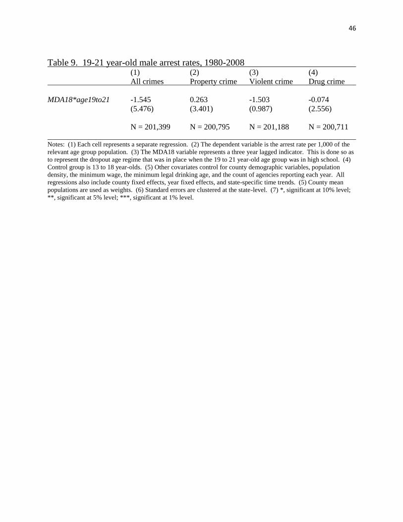
46

Table 9. 19-21 year-old male arrest rates, 1980-2008 (1) (2) (3) (4)


MDA18*age19to21 -1.545 0.263 -1.503 -0.074

(5.476) (3.401) (0.987) (2.556)

N = 201,399 N = 200,795 N = 201,188 N = 200,711

Notes: (1) Each cell represents a separate regression. (2) The dependent variable is the arrest rate per 1,000 of the

relevant age group population. (3) The MDA18 variable represents a three year lagged indicator. This is done so as

to represent the dropout age regime that was in place when the 19 to 21 year-old age group was in high school. (4)

Control group is 13 to 18 year-olds. (5) Other covariates control for county demographic variables, population

density, the minimum wage, the minimum legal drinking age, and the count of agencies reporting each year. All

regressions also include county fixed effects, year fixed effects, and state-specific time trends. (5) County mean

populations are used as weights. (6) Standard errors are clustered at the state-level. (7) *, significant at 10% level;

**, significant at 5% level; ***, significant at 1% level.

47

Table 10. MDA laws and police enforcement, 1982-2005 (1) (2)

Policemen Police expenditures

per capita per capita

MDA17 0.073 -0.299

(0.061) (1.816)

MDA18 -0.014 -10.400***

(0.048) (2.151)

N 1,152 1,058

R2 0.971 0.981

State FE YES YES

Year FE YES YES

State trends YES YES

Notes: (1) Each column is a separate state-level regression. (2) The dependent

variable in the first column is the number of sworn police officers per capita.

The dependent variable in the second column is police protection expenditures

per capita in 2000 dollars. (3) All regression models control for the fraction of

the population aged 15-19, the fraction of the population that is black, the

minimum legal drinking age, state fixed effects, year fixed effects, and state-

specific time trends. (4) State populations are used as weights. (5) Standard

errors are corrected for clustering at the state level. (6) *, significant at 10%

level; **, significant at 5% level; ***, significant at 1% level.

48

Table 11. Do MDA laws displace problems to schools? Evidence from YRBS data (1) (2) (3)

Coefficients on MDA18 Everyone Males Females

Missed school out of fear for 0.032*** 0.019 0.044**

own safety during past month (0.008) (0.018) (0.017)

N 113,727 55,927 57,800

Mean of dependent variable 0.062 0.061 0.063

Had sexual intercourse during 0.025 -0.009 0.061**

past month (0.016) (0.040) (0.025)

N 106,441 51,699 54,742

Mean of dependent variable 0.412 0.419 0.406

Ever been pregnant … … 0.026

(0.018)

N … … 42,303

Mean of dependent variable … … 0.093

Notes: (1) Each cell represents a separate regression. (2) The dependent variable in the top panel is equal to one if

the respondent missed school out of fear for his or her own safety during the past month, and is equal to zero

otherwise. The dependent variable in the middle panel is equal to one if the respondent had sexual intercourse

during the past month, and is equal to zero otherwise. The dependent variable in the bottom panel is equal to one if

the respondent has ever been pregnant, and is equal to zero otherwise. (3) For context, each cell reports the mean

rate for individuals in states with an MDA lower than 18. (4) At the individual-level, all regression models control

for age, grade, and race. All regression models also include state fixed effects, year fixed effects, and state-specific

time trends. (5) Standard errors are clustered at the state-level. (6) *, significant at 10% level; **, significant at 5%

level; ***, significant at 1% level.

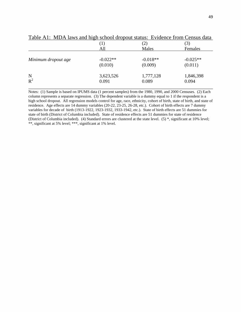
49

Table A1: MDA laws and high school dropout status: Evidence from Census data (1) (2) (3)

All Males Females

Minimum dropout age -0.022** -0.018** -0.025**

(0.010) (0.009) (0.011)

N 3,623,526 1,777,128 1,846,398

R2 0.091 0.089 0.094

Notes: (1) Sample is based on IPUMS data (1 percent samples) from the 1980, 1990, and 2000 Censuses. (2) Each

column represents a separate regression. (3) The dependent variable is a dummy equal to 1 if the respondent is a

high school dropout. All regression models control for age, race, ethnicity, cohort of birth, state of birth, and state of

residence. Age effects are 14 dummy variables (20-22, 23-25, 26-28, etc.). Cohort of birth effects are 7 dummy

variables for decade of birth (1913-1922, 1923-1932, 1933-1942, etc.). State of birth effects are 51 dummies for

state of birth (District of Columbia included). State of residence effects are 51 dummies for state of residence

(District of Columbia included). (4) Standard errors are clustered at the state level. (5) *, significant at 10% level;


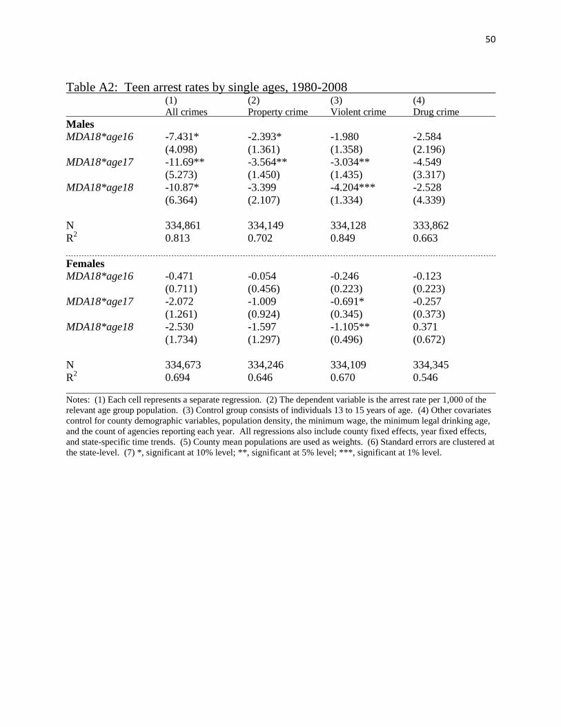
50

Table A2: Teen arrest rates by single ages, 1980-2008

(1) (2) (3) (4)


Males

MDA18*age16 -7.431* -2.393* -1.980 -2.584

(4.098) (1.361) (1.358) (2.196)

MDA18*age17 -11.69** -3.564** -3.034** -4.549

(5.273) (1.450) (1.435) (3.317)

MDA18*age18 -10.87* -3.399 -4.204*** -2.528

(6.364) (2.107) (1.334) (4.339)

N 334,861 334,149 334,128 333,862

R2 0.813 0.702 0.849 0.663

Females

MDA18*age16 -0.471 -0.054 -0.246 -0.123

(0.711) (0.456) (0.223) (0.223)

MDA18*age17 -2.072 -1.009 -0.691* -0.257

(1.261) (0.924) (0.345) (0.373)

MDA18*age18 -2.530 -1.597 -1.105** 0.371

(1.734) (1.297) (0.496) (0.672)

N 334,673 334,246 334,109 334,345

R2 0.694 0.646 0.670 0.546

Notes: (1) Each cell represents a separate regression. (2) The dependent variable is the arrest rate per 1,000 of the

relevant age group population. (3) Control group consists of individuals 13 to 15 years of age. (4) Other covariates

control for county demographic variables, population density, the minimum wage, the minimum legal drinking age,

and the count of agencies reporting each year. All regressions also include county fixed effects, year fixed effects,

and state-specific time trends. (5) County mean populations are used as weights. (6) Standard errors are clustered at

the state-level. (7) *, significant at 10% level; **, significant at 5% level; ***, significant at 1% level.

51

Table A3. Difference-in-difference results, 1980-2008 All crimes

(1) (2) (3)

Males MDA18 -15.23** -15.01* -13.65**

(5.882) (8.170) (5.832)

N 67,282 67,282 67,282

R2

0.898 0.912 0.917

Females MDA18 4.818** -2.534 -3.092

(2.349) (2.634) (2.061)

N 67,296 67,296 67,296

R2

0.702

0.760 0.772

County FE YES YES YES

Year FE NO YES YES

Other covariates NO NO YES

Notes: (1) Each cell represents a separate regression. (2) The dependent

is the arrest rate per 1,000 of the 16 to 18 year-old age group for all crimes (i.e.

property + violent + drug). (3) Other covariates control for county demographic

variables, population density, the minimum wage, the minimum legal drinking

age, and the count of agencies reporting each year. (4) County mean populations

are used as weights. (5) Standard errors are clustered at the state-level. (6) *,

significant at 10% level; **, significant at 5% level; ***, significant at 1% level.

52

Table A4. 19-21 year-old male arrest rates for white collar crimes, 1980-2008 (1) (2) (3)

Forgery Fraud Embezzlement

MDA18*age19to21 0.009 -0.876** 0.008

(0.109) (0.389) (0.020)

N = 132,828 N = 132,872 N = 136,612

Mean = 1.229 Mean = 3.816 Mean = 0.067

Notes: (1) Each cell represents a separate regression. (2) For context, each cell reports the mean arrest rate for 19 to

21 year-olds in states that had an MDA lower than 18. (3) The dependent variable is the arrest rate per 1,000 of the

relevant age group population. (4) The MDA18 variable represents a three year lagged indicator. This is done so as

to represent the dropout age regime that was in place when the 19 to 21 year-old age group was in high school. (5)

Control group is 16 to 18 year-olds. (6) Other covariates control for county demographic variables, population

density, the minimum wage, the minimum legal drinking age, and the count of agencies reporting each year. All

regressions also include county fixed effects, year fixed effects, and state-specific time trends. (7) County mean

populations are used as weights. (8) Standard errors are clustered at the state-level. (9) *, significant at 10% level;


in school and out of trouble? the minimum dropout age and...

Documents