in of geograph - university of toronto t-space · the status of total column ozone concentration...
TRANSCRIPT

Reza Hosseinian
A thesis subrnitted in conforrnity with the requirements for the degree of Master of Science Graduate Department of Geograph y
University of Toronto
O Copyright by Reza Hosseinian (2000)

National Library 1*1 of Canada Bibliotheque nationafe du Canada
Acquisitions and Acquisitions et Bibliographie Services seMces bibliographiques
395 Wellington Street 395. rue Wdlin@Ori Otiawa ON K I A ON4 Ortawa ûbl K I A M Canada canada
The author has granted a non- exclusive licence dowing the National Library of Canada to reproduce, loan, distribute or seil copies of this thesis in microform, paper or electronic formats.
The author retains ownership of the copyright in this thesis. Neither the thesis nor substantid extracts fiom it may be printed or otherwise reproduced without the author's permission.
L'auteur a accordé une licence non exclusive permettant à la Bibliothèque nationale du Canada de reproduire, prêter, distribuer ou vendre des copies de cette thèse sous la fome de microfiche/film, de reproduction sur papier ou sur format électronique.
L'auteur conserve la propriété du droit d'auteur qui protège cette thèse. Ni la thèse ni des extraits substantiels de celle-ci ne doivent être imprimés ou autrement reproduits sans son autorisation.

THE STATUS OF TOTAL COLUMN OZONE CONCENTRATION OVER NORTH AMERICA BY
Rem Hosseinian Graduate Department of Geography
M.Sc. 2000 University of Toronto
Total column ozone concentration measured over North America has been statistically analyzed.
Total column ozone has been decreasing over North Arnerica with strong spatial and temporal
variations. There exist very significant latitudinal variations. Furtherrnore, the existence of
temporal latitudinal variations in total column ozone concentration over the study area is
established. High latitude stations demonstrate an increase in the trend of total ozone
concentration for the period of 1975 to 1985, while midlatitude stations show the largest rate of
total ozone reduction during this period. The rate of total ozone reduction increases during the
period of 1985 to 1995 in high-latitudes, whiIe midlatitude stations demonstrate a slight
decrease in the rate of total ozone reduction. It was also found that quasi-biennial oscillation
(QBO) and solar sunspot activity are the two major sources of long-tem natural total column
ozone variations over the study area. The effect of these mechanisms is more pronounced in
high latitudes than elsewhere. Finally, it was determined that ozone data from the ground-based
stations are representative of an area approximately 1S0 in radius.

1 wish to express my gratitude to a number of individuals for their comrnents and
guidance at various stages in preparation of this thesis. First and foremost, I'm gratefui to my
supervisor Dr. W. Gough for his instruction, careful editing, support, and encouragement
throughout the course of this study. Not only you have k e n a great inspiration throughout my
University career, but you have also been a good friend. Special thanks goes to my friends and
colleagues at the Climate Lab, each of whom catalyzed my research in one way or another, and
made the p s t 3 years fun and exciting. 1 gratefully acknowledge support from the World Ozone
and Ultraviolet Radiation Data Center of Environment Canada, National Geophysical Data
Center, and the Institute of Meteorology at the Free University of Berlin for their compilation of
data used in this study. Further thanks goes to the members of the defense cornmittee, Dr. Tony
Pnce and Dr. Brian Greenwood for participating in the improvement of this report.
Appreciation is also due to Professor Aysha Hashim for sharïng her expertise in statistical
methods. This paper benefited from programming assistance provided by Dara Jahani.
A very special and heartfelt thanks goes to my two dear friends Houman Abrisharnkar
and Jackie Missaghi for their continuous moral and emotional support over the years. Thank
you for always being there for me,
1 sincerely thank my dear parents, M. Javad Hosseinian and Mrs. Maryarn Hosseinian
for their constant love and encouragement, and for supporting me in al1 my endeavors. This
work is dedicated to my parents.
The funding for this research was in part supported by the National Science and
Engineering Research Council of Canada (NSERC) and Student Career Placement (SCP).
iii

. . Abstract ............................................................................................................................................ ... ......................................................................................................................... Acknowledgments iii
Table of Contents ........................................................................................................................ iv List of Tables ............................................................................................................................... vi . . List of Figures .............................................................................................................................. vit
Chapter 1 ...................................................................................................................................... 10 ...................................................................................................................... . 1 0) Introduction 10
1 -1 ) Techniques of Observing Atmospheric Ozone ........................................................... 13 1 -3 ) Formation and Destruction of Ozone in the Stratosphere ..................................... 14 1.3) Total Ozone Distribution ....................... ... ............................................................. 16 1 A) The influence of Dpamical Processes on Ozone Abundance .................................... 18
1.4.1) The Dynamical Structure of the Stratosphere ...................................................... 19 1.4.2) The Global Structure of Ozone Transport and Mixing ........................................ 21
1.5) S tratospheric Ozoae Perturbations ............. ..... ............................................... 2 3 ..................................................................................... 1 .5 . 1) Solar-induced Variations 23
........................................................................... L -5 -3) Volcanic-induced Variations 2 6 1 S.3) Quasi-Biennial Oscillation induced Variations .................................................... 27
. - ............................................................................. 1.5.4) El Nino-induced Variations 3 1 ................................................................................................... 1.6) Trends in total Ozone 32
1.6.1) The Role of Heterogeneous Chemistry on Midlatitude Ozone Depletion ........... 33 1-62) The Role of Cirrus Clouds on Midlatitude Ozone Depletion .............................. 36 1.6.3) The Possible Role of Iodine on Midlatitude Ozone Depletion ............................ 38 1.6.4) The Possible Role of Aircraft-generated Soot on Midlatitude Ozone depletion - 4 1 1 . 6 . The Role of Polar Regions on Midlatitude Ozone Depletion .............................. 43
............ 1 . 6 . The Role of Dynarnical Contributions on Midlatitude Ozone Depletion 45 1.7) Objectives .................................... ... ............................................................................. 48
...................................................................................................................................... Chapter 2 49 2.0) Data Sources and Analysis Methods ................................................................................ 49
2.1) Source of Data .............................................................................................................. 49 2.1.1) Total Column Ozone Data ................................................................................... 49 2.1.2) SolarSunspotData ............................................................................................... 51
............................................................................................................. 2.1.3) QBO Data 52 2.2) Statistical Analysis ..................................................................................................... 52
.................................................................................. 2.2.1) Daily Total Column Ozone 52 2.2.2) Time Senes and Linear Regression Anal ysis ......................... .... ...-.-...... 53 2.2.3) Pearson's r Correlation Analysis ......................................................................... 53 2.2.4) Spectral and Cross-Spectral Anal ysis .................................................................. 55
........................................................................................................ ..................... Chapter 3 ... 58 3.0) Results and Discussion .................................................................................................. 5 8
3.1) Analysis of secular trends of total ozone over Canada and the United States .................. 58 3.1.1) Spatial Variation ........................................................................................................ 58
....................................................... ..................................... 3.1.2) Temporal Variation .. 69 3.2) Total Column Ozone Concentration: How Representative is Toronto of North
.................................................................................................................................. Amenca? 74 ....... 3.3) Spectral Analysis: What are the non-anthropoeenic sources of ozone variation? 78

....................................................................... 3.3.1) Seasonal Decomposition Methods 79 3.3.2) Long-Term Cycles Present in Total Column Ozone Data ................................... 85 3.3.3) Spatial Variations Resulting from Non-anthropogenic Sources Responsible for Natural Variability of Ozone ................................................................................................ 93
Chapter 4 ...................................................................................................................................... 96 ................................................................................ 1.0) Conclusions and Recomrnendations 96
......................................................................................................................... 5.0 References 100 Appendix a) Detemination of Total Column Ozone ................................................................. 107
............................................................................................ 1) Dobson Spectrophotometer 107
............................................................................................ 2) Brewer Spectrophotometer 109 3) M-83 Ozonorneter .......................................................................................................... 110
....................................................................................................... 4) Satellite Techniques I l l ......................................................... 5) Determination of the Vertical Ozone Distribution 112
Appendix B) Photo-oxidation Pathways Between Active Ozone Destroying Radicals and ....................................................................................................................... Reservoir species 113
1) HO, Chemistry ............................................................................................................... 113 ............................................................................................................... 2 ) NOx Chemistry 115
............................................................................................. 3) CIO, (Halogen) Chemistry 116 .......................................................................... 4) Coupling of HOx/NOx/CIOx Reactions 118
.......................... 5) SO, Chemistry .. ............................................................................... 119 ........................................... 6) High-Latitude Ozone Loss and Heterogeneous Chemistry 120
6.1) Sulfate Aerosol Chemistry .............................................................................................. 121 ............................................................................. 6.2) Polar Stratosphenc Cloud Chemistry 122
TabIe 2.1 : A summary of WOUDC stations used ........................................................................ 51
......................................................... TabIe 3.1.1 : A summary of figures 3.1.2. 3.1.3. and 3.1.4. 62
Table 32.1: Results of Pearson correlation analysis between station 65 and other stations over North America ..................................................................................................................... 75
Figure 1.4.1 : Schematic illustration of the Brewer-Dobson circulation, proposed to account for the observed distribution of various conserved trace constituents in the lower stratosphere
37 (James, 1994). Arrows indicate direction of transport ................................................... -- Figure 1 S. 1 : Time senes of solar sunspot cycles from 1960 to 1999. ....................................... 25
Figure 1.5.2: Time series of the monthly-mean zona1 wind (30-mb) measured at Singapore (1.3"N) during the penod 1960 to 2000. This diagram demonsuates the equatonal QB0.28
Figure 2.0.1: The study area (the satellite image is provided by map.com, 2000) ..................... 50
Figure 3.1.1: The approximate !ocation of the stations and transects A, B, and C (the satellite image is provided by map.com, 2000). ............................................................................. 5 9
Figure 3.1.2: Total monthly ozone concentration for stations in transect A. The station id, latitude and longitude coordinates, and the equation of the line of best fit (the regression coefficient is underlined), is provided above each graph. The confidence level of the regression coefficient is greater than 99.9% for each of the four stations (highly significant). .......................................................................................................................... 60
Figure 3.1.3: Total monthly ozone concentration for stations in transect B. The station id, latitude and longitude coordinates, and the equation of the line of k s t fit (the regression coefficient is underlined), is provideti above each graph. The confidence level of the regression coefficient is 64% for station 51 (not significant), greater than 99.9% for station 24 (highly significant), and 97% for station 199 (statistically significant) .......................... 60
Figure 3.1.4: Total monthly ozone concentration for stations in transect C. The station id, latitude and longitude coordinates, and the equation of the line of best fit (the regression coefficient is underlined), is provided above each graph. The confidence level of the regression coefficient is greater than 99.9% for each of the four stations (highly significant). .......................................................................................................................... 6 1
Figure 3.1.5: Absolute ozone concentration and % of ozone lost (per decade) vs. latitude. ....... 66
Figure 3.1.6: Total monthly ozone concentration for periods of 1965 to 1975, 1975 to 1985, and 1985 to 1995. The station identification, latitude and longitude coordinates, equation of the line of best fit (regression coefficient is underlined), and the confidence level of the regression coefficient is provided for each station ............................................................. 70
Figure 3.2.1: A contour map of 8 vs. relative Latitudehngitude. Blue represents a hundred percent correlati on (Toronto) or ?= 1. Relative latitude and longitude represent degrees away from station 65 which is located in Toronto. The gridding technique used is "the inverse distance to a power of 3" method. The results are only significant within the
.................................................................................................................... rectanoular u box. 76
Figure 3.3.1 : Spectral anal ysis of monthl y total column ozone data for station 65, Toronto, Canada. ................................................................................................................................ -79
Figure 3.3.2: Range of Total column ozone concentration (ieft vertical axis) and Mean column ozone concentration (right vertical axis) vs. Time for station 65, Toronto. This figure
............................................................................ shows that ozone data is multiplicative 8 1
Figure 3.3.3: Spectral analysis of seasonally adjusted monthly total colcmn ozone data for station 65, Toronto, Canada. Note: the seasonal cycIe (fS.083) is still present. ............... 82
Figure 3.3.4: Spectral analysis of monthly total column ozone data (with 13-month running mean rnethod applied) for station 65, Toronto, Canada. Note: the seasonal cycle (f=0.083) is stilI present but is much wedcer. ...................................................................................... 83
Figure 3.3.5: Spectral anaiysis of rnonthly total column ozone data (with 13-month running mean rnethod applied and only half a weight given to the first and the last months) for station 65, Toronto, Canada. Note: the seasonal cycle (fa.083) is completely removed.. 84
Figure 3.3.6: Spectral analysis of monthly total column ozone data (with 13-month running mean method applied) for station 65, Toronto, Canada, The red arrows represent QBO cycIes, the green arrow represents the solar cycle, the blue arrow represents the length of the data, and the black arrow is the unknown trend in the data (potentially related to El Nifio/Southern Oscillation phenornena) or perhaps noise. .............................................. 86
Figure 3.3.7: Time senes of solar sunspot number ( k f t axis: light blue represents the actual sunspot numbers and the dark blue is the smoothed seriesj and totaI column ozone concentration (Right axis: 13rnonth running mean applied and detrended) for station 65, Toronto. The two major volcanic eruptions are marked. ............................................... 86
Figure 3.3.8: Spectral analyses of monthly solar sunspot number from 1960 to 1999. The major spectral density peak is at f=0.008288, or 10 years. ...................................................... 8 7
Figure 3.3.9: Cospectrum of monthly solar sunspot number and total column ozone concentration (station 65, Toronto) from 1960 to l999. ...................................................... 87
Figure 3.3.10: Phase spectrum of monthly solar sunspot number and total column ozone concentration (station 65, Toronto) from 1960 to 1999 .................................................-..... 88
Figure 3.3.1 1 : Coherence spectrum of monthly solar sunspot number and total column ozone concentration (station 65, Toronto) from 1960 to 1999 ....................................................... 88
Figure 3.3.12: Time series spectral analyses of Singapore zonal wind (QBO) at 30-mb, from 1960 to 1999. ....................................................................................................................... 90
Figure 3.3.13: Cospectrum of mean monthly total ozone (station 65, 13-month running mean applied) and Singapore zona1 wind (QBO) at 30-mb, from 1960 to 1999 ........................... 90
... Vl l l
Figure 3.3.14: Phase spectrum of mean monthly total ozone (station 65. 13-month running mean applied) and Singapore zona1 wind (QBO) at 30.mb. from 1960 to 1999 ........................... 91
Figure 3.3.15: Coherence spectrum of mean monthly total ozone (station 65. 13-month mnning mean appIied) and Singapore zona1 wind (QBO) at 30.mb. from 1960 to 1999 ................. 91
Figure 3-3-16: Spectral analyses for some of the stations dong Transects A. B. and C .............. 94

O zone (O3), a variable trace constituent of the earth's atmosphere whose early
o e i n is closely linked with that of atmospheric oxygen (O,) and water vapor
(HzO), is a molecule composed of 3 oxygen atoms capable of absorbing certain
wavelengths of biologically damaging ultraviolet light. It is the only gas in the atmosphere that
possesses such capability and, therefore, is an essential part of the Earth's ecological balance.
The evolution of Iife on earth is closely tied to the formation of the protective ozone layer
(Kowalok, 1993).
When, some 3 billion years ago, life on Earth started to produce oxygen via
photosynthesis, a decisive step was taken in the evolution of the Earth's atmosphere (Peter,
1994). The presence of oxygen initially resulted from photo-dissociation of water vapor, out-
gassed from the interior of the earth and from recoinbination of water vapor and carbon dioxide
in the presence of sunlight (London and AngeIl, 1982). For a long time most of this oxygen was
used up in iron and sulphur oxidation processes, and it was only about 2 billion years BP that
accumulation of additional free oxygen in the atmosphere began. This became more rapid after
the colonization of the continents and reached the present level ( ~ 2 1 % ) about 350 million years
BP. Life was able to forsake the refuge offered by the oceans and to emigrate to the continents
because the increasing atmospheric oxygen levels absorbed the short-wavelength ultraviolet
(UV) radiation and produced ozone (Peter, 1994). As the oxygen concentration increased to its
present value, the amount of ozone also increased and the level of maximum concentration rose
to its present average height of about 25 km (London and Angell, 1982). This build-up of
atmospheric ozone led to a further reduction in the penetration of harrnful UV radiation in
longer wavelength regions as well, causing improved conditions for higher forms of life on
Earth (Peter, 1994).
Although molecular nitrogen and oxygen were discovered as early as 1774, the
recognition of ozone as a distinct chemical species came only after the advent of controlled
electric energy. The Dutch scientist Van Marum was the first to observe that a peculiar odor
resulted from passing an electrical discharge through oxygen. The substance causing the odor
was identified in the faboratory by the Swiss chemist Schonbein, who noted that the same strong
odor occurred in oxygen generated from the electrolysis of water and in air when the y were
subjected to an electric discharge. He suggested that the substance might be a permanent feature
of the atmosphere and thus deserved a narne: he proposed that it be called ozone (probably after
the Greek word ozierr = to smell). More precise knowledge of the origin of ozone was obtained
a few years later when de Ia Rive and Marignae demonstrated its production by electric
discharge in pure and dry oxygen. The first chernical identification of ozone was probably due
to Soret who stated that "la molécule d' ozone fût composée de 3 atomes 000 et constituât un
bioxyde d'oxygene" (Whitten and Prasad, 1985 and references therein).
Because ozone was known to be produced efficiently by electric discharge, including
lightning, the early belief was that ozone is distributed close to the earth's surface. Hartley
(1 88 1) was the first to point out that ozone is a normal constituent of the higher atmosphere and
that it is in larger proportion there than near the earth's surface. The first satisfactory
determination of the height of the absorbing medium was given by Lord Rayleigh (Strutt, 1918)
who based his estimate on observations of the solar spectrum at sunrise and sunset. He
concluded that atmospheric ozone is largely confined to a layer between 40 to 60 km above sea
level. Because of limitations of the experimental method, his estimate was only qualitatively
correct. Later, geatly improved measurements by Gotz et al. (1 934) established the presently

accepted bounds to the stratospheric ozone Iayer, 10 km to 50 km altitude with a maximum
concentration occumng near 25 km. Regener and Regener (1934) confirmed the Gotz et al.
( 1933) measurements by making direct spectrographie observations from a balloon that
ascended to 3 1 km. The measured solar ultraviolet spectrum showed clearly that ascent through
the ozone layer resulted in gradua1 extension of the spectrum toward the ultraviolet (Whitten and
Prasad, 1985 and references therein).
Presently, it is well known that most of the world's ozone (= 90%) is found in the
stratosphere (Kowalok, 1993). As mention earlier, the significance of this layer is its strong
absorption of ultraviolet radiation. The absorption is essentially complete between 200 and 290
nm and less strong in the 290-330 nm region. The heat from this absorption causes the
temperature to increase with altitude. This inverted temperature profile is largely responsible
for the dynamic stability of the stratosphere (Shen et al., 1995). The UV radiation of most
concern is usually referred to as UV-B and includes light with wavelengths between 280 and
3 10 nm. This radiation can cause sunburn and certain skin cancers. The effectiveness of this
radiation in changing biological matenal suggests that almost any living tissue exposed to it
suffers some effect (Firor, 1990). Hence, the presence of the stratospheric ozone layer is vital
both to human health and to the dynamic stability of the stratosphere.

Measurements of the total arnount of ozone in a vertical atmospheric column, whether
made from ground or from satellite-based instruments, depend on optical techniques. Ground-
based methods make use of radiance measurements from an extemal light source like the sun or
the moon after the radiation has suffered extinction as a result of atmosphenc absorption,
rnolecular scattering, and large particle (aerosol) scattering, al1 of which are wavelength-
dependent. Satellite measurements, on the other hand, are based on the extinction of upwefling
radiation whose source is either backscattered soiar radiance or infrared emittance from the
earth-atmosphere system (London, 1985).
The first technique for measuring the total abundance of ozone in a vertical column was
suggested by Fabry and Buisson (1921). Dobson and Harrison (1926) refined the method and
developed instrumentation capable of making precise measurements. PresentIy, their technique
is the standard for making ground-based measurements of total ozone. The Dobson instrument
measures relative intensities at different waveIengths in the spectral range 300-340 nm after
passage of the radiation through the atmosphere. From the data obtained, the ozone column
density is deduced. The data analyses presented in Section 3 are based on total column ozone
measurements made using a network of Dobson Spectrophotometers operated by WMO.
Ozone observations are also made with a broad-band optical filter, mainly in the Soviet Union
and Eastern Europe. However, those data are not always in agreement with Dobson data taken
at the same place and do not seem to be as precise as the latter. For these reasons, only the
Dobson instrument at Boulder, Colorado has k e n accepted as the international standard
(W hi tten and Prasad, 1985 and references therein).
Techniques have also been developed to measure ozone in situ from aircraft and balloon
platforrns. These methods use a wet chemical system in which ozone reacts with a chemical
(potassium iodide) in solution, or a gas phase system in which the reactions produce
chemiIuminescence of which the intensity can be measured, and are used to measure the vertical
distribution of ozone. The most recent developments employ satellites that either measure the
spectral radiance of backscattered soIar ultraviolet (BUV) radiation or limbscan in which the
absorption of solar radiation over an appropriate spectral segment is measured (Whitten and
Prasad, 1985 and references therein). Details are presented in appendix (A).
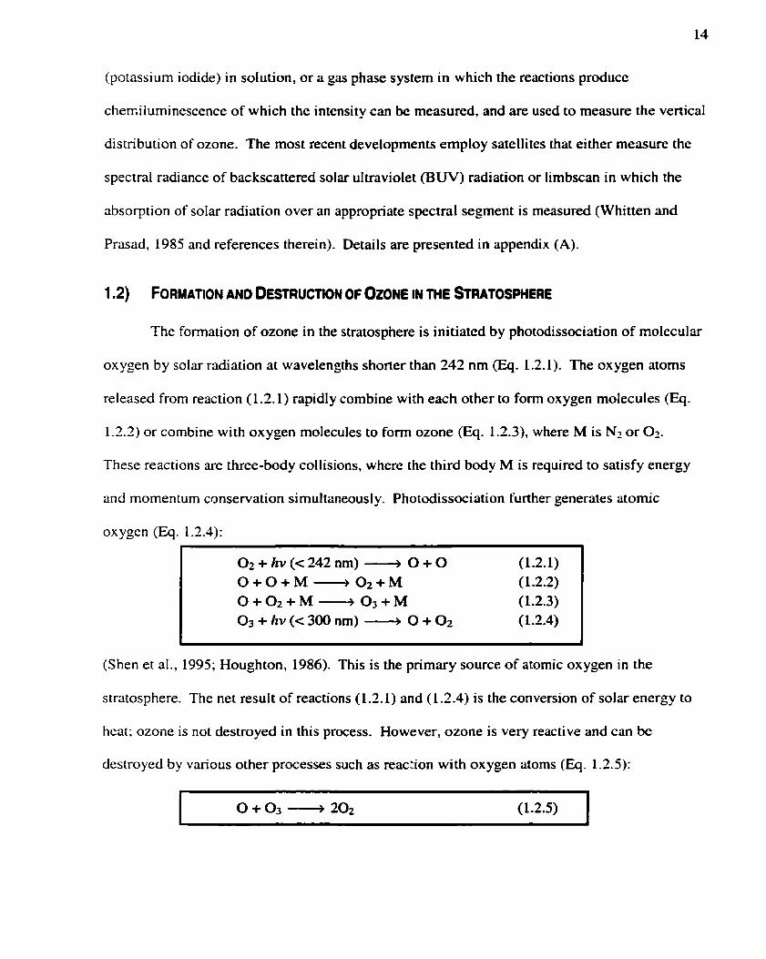
1.2) FORMATION AND DESTRUCT~ON OF OZONE IN THE ~"~RATOSPHERE
The formation of ozone in the stratosphere is initiated by photodissociation of molecular
oxygen by soin radiation at wavelengths shorter than 242 nm (Eq. 1.2.1). The oxygen atoms
released from reaction (1 -2.1) rapidly combine with each other to form oxygen molecules (Eq.
1.2.2) or combine with oxygen molecules to form ozone (Eq. 1.2.3), where M is NI or 01.
These reactions are three-body collisions, where the third body M is required to satisfy energy
and momentum conservation simulta~eously. Photodissociation futher generates atomic
oxygen (Eq. 1.2.3):
I O2 + hv (< 242 nm) --4 O + O (12.1) 1 O + O + M ---, O t + M (1.2.2) O + 0 2 + M + 0 3 + M (1.2.3) O3 + hv (< 300 nm) -+ O + O2 (1 .2.4)
(Shen et al., 1995; Houghton, 1986). This is the primary source of atomic oxygen in the
stratosphere. The net result of reactions (1.2.1) and (1.2.4) is the conversion of solar energy to
heat; ozone is not destroyed in this proçess. However, ozone is very reactive and can be
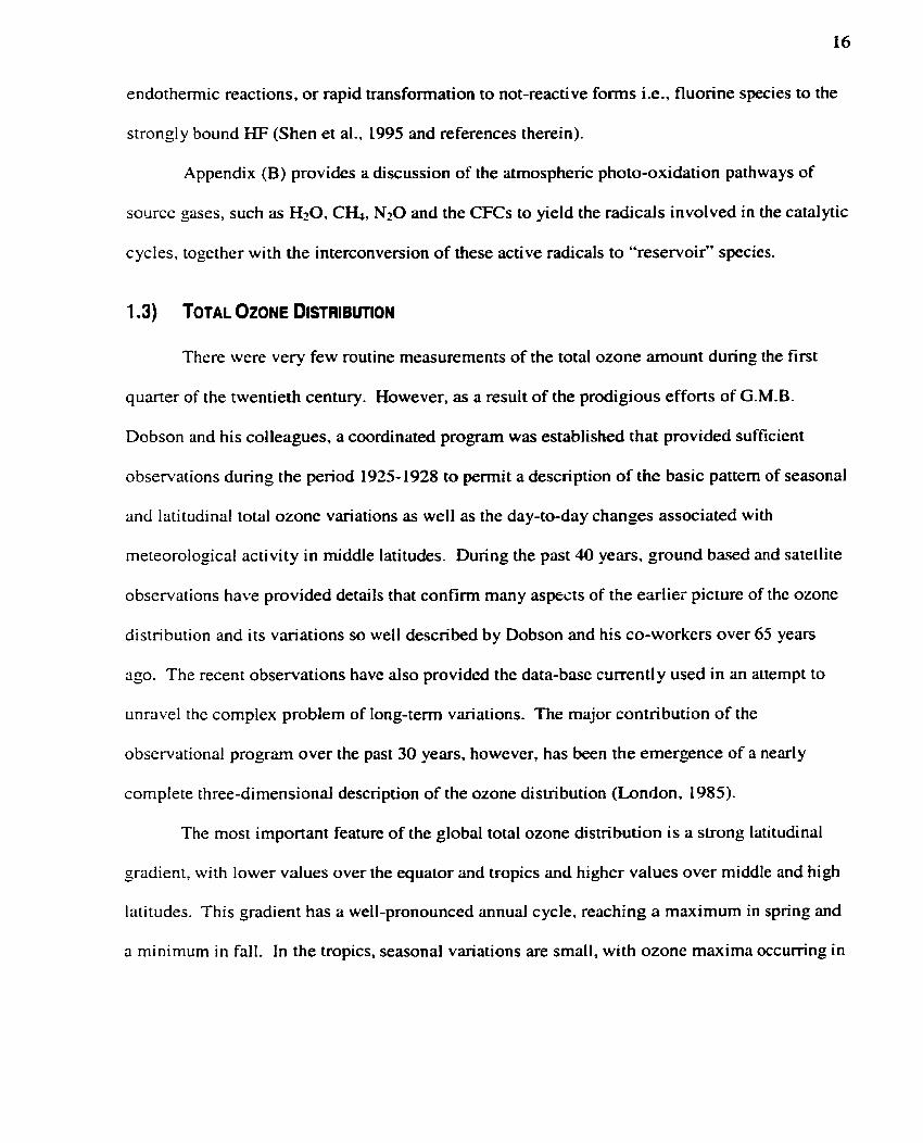
destroyed by various other processes such as reac:.ion with oxygen atoms (Eq. 1.2.5):
which converts "odd9'-oxygen (defined as the sum of ozone and atornic oxygen) back to "evenV-
oxygen, O?. Normal ozone abundances peak in the 6-8 ppm range at an altitude around 20-25
km. Globally averaged column arnounts, i.e. vertical integrds, typically Vary from 290 to 3 10
Dobson units (Shen et ai., 1995). One Dobson Unit Le. DU, is defined as 0.01 mm atmospheric
thickness at STP i.e. zero degrees Celsius and 1 atrnosphere pressure.
The above five steps form the model proposed by Sidney Chapman in 1930. For 20
years this simple model, involving only oxygen species, appeared sufficient to explain the
balance between the production and destruction of ozone in the stratosphere. It is of interest to
note that in the dark, such as during the polar night, there should be no production or destruction
of ozone according to this mechanism (Shen et al., 1995).
Refinements in measurements revealed that ozone abundances were noticeably smaller
than those predicted by Chapman's reactions. In the 1950s and 1960s other ozone destruction
path ways were proposed, based on the photocherni stry of atmospheric water and the influence
of the reactive radicals on the distribution of odd-oxygen in the atmosphere. More recently the
importance of nitrogen oxides and chlorine compounds have become apparent, and of great
concern owing to the anthropogenic perturbations in the concentrations of these chemicals in the
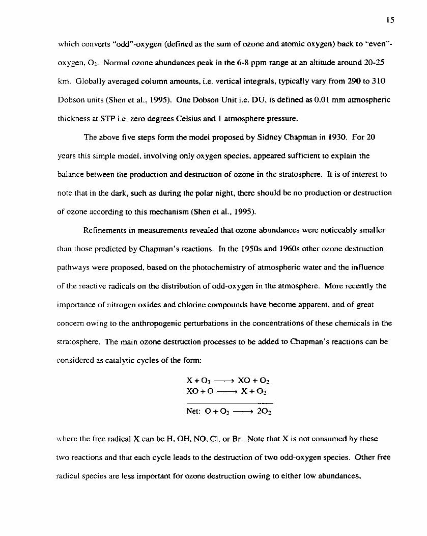
stratosphere. The main ozone destruction processes to be added to Chapman's reactions can be
considered as catalytic cycles of the fonn:
Net: O + O3 + 202
where the free radical X can be H, OH, NO, CI, or Br. Note that X is not consumed by these
two reactions and that each cycle leads to the destruction of two odd-oxygen species. Other free
radical species are less important for ozone destruction owing to either low abundances,
endothermic reactions, or rapid transformation to not-reactive forms Le., fluorine species to the
strongly bound HF (Shen et al., 1995 and references therein).
Appendix (B) provides a discussion of the atmospheric photo-oxidation pathways of
source gases, such as H20, C a , N20 and the CFCs to yield the radicals involved in the catalytic
cycles, together wi th the interconversion of these active radicals to "reservoir" species.
There were very few routine measurements of the total ozone amount during the first
quarter of the twentieth century. However, as a result of the prodigious efforts of G.M.B.
Dobson and his colleagues, a coordinated program was established that provided sufficient
observations during the period 1925-1928 to permit a description of the basic pattern of seasonal
and lati tudinal total ozone variations as well as the day-to-day changes associated with
meteorological activity in middle latitudes. During the past 40 years, ground based and satellite
observations have provided detaits that confirm many aspects of the earlier picture of the ozone
distribution and its variations so well described by Dobson and his CO-workers over 65 years
ago. The recent observations have also provided the data-base currently used in an attempt to
unravel the complex problem of long-term variations. The major contribution of the
observational program over the past 30 years, however, has been the emergence of a nearly
complete three-dimensional description of the ozone distribution (London, 1985).
The rnost important feature of the globaI total ozone distribution is a strong latitudinal
gradient, with lower values over the equator and tropics and higher values over middle and high
latitudes. This gradient has a well-pronounced annual cycle, reaching a maximum in spring and
a minimum in faII. In the tropics, seasonal variations are small, with ozone maxima occumng in

summer. In the equatorid region, there are essentially no seasonal variations (Environment
Canada, 1999).
The explanation for this behaviour, also deduced by Dobson and confirmed by Brewer
from aircraft measurements of water vapour, is that the high values at extra-tropical latitudes are
a result of transport of ozone from the region of primary production in the equatorial middle and
upper stratosphere to the lower stratosphere in polar regions, where it has a relatively long
photochernical relaxation time. Ozone is formed, primarily in the tropics at altitudes above
about 30 km, via the action of ultraviolet light from the Sun upon molecuiar oxygen (Section
1.2). While the highest relative concentrations are found here, the more moderate values of 1-2
ppmv found at about 15 km altitude, actually make a much greater contribution to the total
column ozone, because the density of the atmosphere is greater by an order of magnitude at the
lower altitude. Mixing ratios in the lower stratosphere are higher at midlatitudes and toward the
poles. This latitudinal distribütion is made possible by the relatively long lifetime (months to
years) of ozone in the lower stratosphere, and the Brewer-Dobson circulation (see Section 1.4.2)
that transports stratospheric ozone from the tropics toward the poles and downwards at high
latitudes. This circulation is both strongest and most variable in winter, and the highest total
colurnn amounts and the most variability are found in the winter stratosphere below 20 km
(Environment Canada, 1999; London, 1985).
The pronounced annual variation of total ozone is strongly latitude dependent. The
phase of the annual variation reaches a maximum in mid-March at northem subpolar latitudes, is
delayed to early April at midlatitudes, and further delriyed to early June near the equator. The
mid-March maximum results from the transport of ozone toward higher latitudes by the large-
amplitude stationary waves in the stratosphere. In spring, when the latitudinal temperature

gradient decreases, the amplitude of the stationary waves is much srnaller and the poleward
ozone transport is wedcened (London, 1985).
In addition to the strong ozone dependence on latitude, there is a longitude variation that
is most apparent in the Northem Hemisphere and is best developed during the late winter and
early spring. The variation is such that high ozone amounts are generally found at longitudes
corresponding to upper-level trough positions and vice versa. This relationship is rnuch more
pronounced during wintedspring when the circutation systems in the lower and middie
stratosphere are closely linked and affected by surface topography (London. 1985 and
references therein).
Harrnonic components of the observed longitude variation of ozone have been computed
and the results indicate that wave number one is dominant at high latitudes during the winter in
the Northem Hemisphere and the spring in the Southern Hemisphere. Wave numbers two and
three are signifiant only at rnid and subpolar latitudes in the Northem Hemisphere dunng the
winter and spring. In summer and early fa11 the stratospheric latitudinal temperature gradient is
reversed and the stratospheric winds are strongly zona1 (from the east) and oniy minirnally
related to topographically induced standing waves. Thus, longitude variations in ozone during
the summer are small (London, 1985 and references therein).
1.4) THE INFLUENCE OF DYNAMICAL PROCESSES ON OZONE ABUNDANCE
Dynamical processes affect ozone abundance in two important ways: first, through
temperature and, second, through transport and mixing. Although the two aspects are related in
practice Le., the same dynamical processes that control transport and mixing affect temperature;
i t is useful to maintain a distinction (Environment Canada, 1999).
1.4.1) The nvn&sl Structure of the S t r w e r e
The stratosphere contains roughly 20% of the mass of the atmosphere. It is
distinguished by a strong vertical stratification, or layering, that inhibits venical motion. The
existence of the stratosphere is a consequence of the ozone layer. Although the strongest heating
of the atmosphere occurs at the earth's surface, there is a secondary heating maximum
throushout the czone layer. Rapid vertical heat transfer by convection in the lowest part of the
atmosphere, referred to as convective adjustment, leads to a layer of weak stratification (the
troposphere), capped by a layer of strong stratification (the stratosphere). The boundary
between the two is the tropopause. The global mean height of the tropopause is thus determined
by a balance between the amount of stratospheric ozone, the surface temperature, and the
vertical temperature structure of the troposphere (which involves the distribution of water
vapour and clouds). It follows that changes in any of these quantities can be expected to !ead to
changes in the global mean height of the tropopause (Environment Canada, 1999).
The height of the tropopause varies significantly with latitude. It is greatest in the
tropics, where it is typically around 18 km, and decreases to around 8 km at the poles. Part of
this variation can again be explained on radiative-convective grounds: since surface heating is
strongest in the tropics, the depth of convective adjustment is greater there. However, there are
two other contributing effects that act in the same direction. First, there is a persistent mean
meridional mass circuIation in the stratosphere that draws air upward in the tropics and pushes it
downward in the extratropics (see Section 1.4.2). Second, although the photochemicat
production of ozone takes place primarily in the tropics, significant quantities of ozone are
transported poleward, thus affecting the latitudinal distribution of radiative heating. Both effects
- which are closely related (see Section 1.4.2) - act to raise the tropopause in the tropics and to
lower it in the extratropics. In addition, there is a sharpening of the tropopause slope in

midlatitudes associated with the subtropical jet stream, which is controlled by tropospheric
synoptic-scale weather systems. Thus, the latitudinal structure of the tropopause reflects a
complex interplay between the mass circulation of the stratosphere, the ozone distribution,
upper-tropospheric synoptic-scale disturbances, and the latitudinal temperature gradient of the
lower troposphere (Environment Canada, 1999).
There is a very direct connection between the spatial distribution of ozone and the spatial
structure of the tropopause. Generally, comparatively high vaiues of ozone are found in the
stratosphere, and comparatively low values are in the troposphere. On short timescales (Le.,
several days), the tropopause acts as a defonnable material surface. When the tropopause
descends, the fraction of stratospheric air above that location increases, thereby increasing total
ozone; when the tropopause ascends, there is a corresponding decrease in total ozone. This
correlation is well established on short timescales associated with dynamical variability in the
tropopause height (Environment Canada, 1999).
The elevated tropical tropopause implies that a local minimum in lower stratosphere
temperatures will occur in the tropics - the reverse of the situation in the troposphere. This
feature is present in al1 seasons and is associated (via thermal-wind balance) with the subtropical
jet stream. At higher altitudes, the latitudinal temperature structure has a drarnatic seasonal
dependence. Ozone that has been transported poleward provides a major source of radiative
heating in the sunlit polar summer, which maintains the relative warmth of polar temperatures
relative to tropical values. In the winter hemisphere, in contrast, the lack of radiative heating
over the polar night leads to extremety low temperatures and the formation of an intense
westerly polar vortex. Thus, in polar-regions, the seasonal cycle of temperature consists of a
cooling trend in the faIl and a warming trend in the spting. The low temperatures of the polar
night, however, are mitigated by adiabatic heating arising from the compression of the
descending, poleward-moving air (Environment Canada, 1999).
1 A.2) The Global Structure of Ozone Trawort and Wing . .
In the upper stratosphere, at heights between 30 and 50 km, atmospheric motions have
hardly any influence on the large-scale distribution of ozone. At these levels, the ozone
concentration reaches its photochemical equilibrium in quite a short tirne, certainly short
compared to the time for atmospheric motions to advect ozone to regions where the temperature,
pressure or radiative regime is significantly different. In the lower stratosphere, the
photochemical reaction rates become smail, and so the tirne required to reach photochemical
equilibrium becomes several weeks, much longer than the typical dynamical timescale. In the
lower stratosphere, then, ozone is advected around almost as a conserved tracer. In fact, the
largest abundances of ozone are found in the lower stratosphere, suggesting that the transport of
ozone from production regions is a very important process. Furtherrnore, the column integrated
ozone amount is a maximum at high latitudes in the spnng, where photochemical production
rates would be expected to be very Iow; there are simply not enough sufficiently energetic
photons available to produce the observed abundances of ozone. Once more, there must be
signifiant transport of ozone from lower latitudes (James, 1994).
The Brewer-Dobson circulation was proposed in the 1940s to account for the observed
distri bution of ozone and other conserved trace constituents in the lower stratosphere. It is
illustrated in Figure 1.4.1 and consists of a meridional circulation in each hemisphere, with air
rising into the stratosphere in the tropics, rnoving poleward, with descent and entrainment back
into the troposphere at high latitudes. Such a mass circulation will transport ozone from the
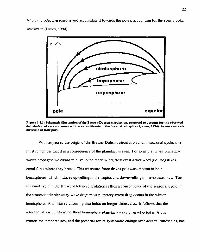
tropical production regions and accumulate it towards the poles, accounting for the spring polar
maximum (James, 1994).
troposp here I I
pole equatot
Figure 1.4.1: Schematic iiiustration of the Brewer-Dobson circulation, pro- to account for the observed distribution of various conserveci trace constituents in the bwer stratosphere (James, 1991). Arrows indicate direction of transport,
With respect to the origin of the Brewer-Dobson circulation and its seasonal cycle, one
must remember that it is a consequence of the planetary waves. For example, when planetary
waves propagate westward relative to the mean wind, they exert a westward (i.e., negative)
zona1 force where they break. This westward force drives poleward motion in both
hernispheres, which induces upwelling in the tropics and downwelling in the extratropics. The
seasonal cycle in the Brewer-Dobson circulation is thus a consequence of the seasonal cycle in
the stratospheric planetary-wave drag; most planetary-wave drag occurs in the winter
hemisphere. A similar relationship also holds on longer timescaIes. It follows that the
interannual variability in northern hemisphere planetary-wave drag reflected in Arctic
wintertime temperatures, and the potential for its systematic change over decadal timescales, has

concomitant implications for variability and change in the Brewer-Dobson circulation and hence
in the ozone distribution (Environment Canada, 1999 and references therein).
Damage to the ozone layer by human activity is complex and completely invisible to
anyone but the scientists who are studying the issue. Yet, around the world, people who thirty
years ago had never hear the word ozone are now worried about its disappearance (Firor, 1990).
Intensive theoretical and experimentd investigations of stratospheric ozone have been
undenvay for decades. The aim of the work is to elucidate the formation mechanisms and
meteorology of the background ozone layer, the factors that can lead to ozone change, and the
biological and climatological implications of ozone alterations. The wide spectrum of natural
spatial and temporal fluctuations in ozone concentrations must be taken into account in gauging
human impact (Turco, 1985). There are a large number of natural factors such as solar
variations, volcanoes, quasi-biennial oscillation (QBO), and El Niiïo that affect natural ozone
levels.
1.5.1) Sglar-inQyced V ~ o n ~ m .
Obseneations of variations in the sun's appearance have k e n documented from as long
ago as - 1200 BC during the Shang Dynasty in China, and a pupil of Aristotle provides the
earlies t known reference to a sunspot. Consistent observations have been possible since the
bcginning of the telescopic era around 1610, Galileo perhaps being the first to observe a sunspot
through a telescope (Waple, 1999).
Sunspots are dark areas seen on the photosphere (the visible solar disk). There is yet no
universally accepted explanation for the existence of these sunspots though they are
acknowledged to be magnetic anomalies and, as they increase in number, they appear to reduce

the sun's irradiance. The reduced irradiance due to sunspots is more than compensated for by
corresponding bright areas (plages or faculae) on the photosphere at times of high solar activity
(sunspot maxima), so that at such times the sun's total irradiance is actually greater by a factor
of 1.5. Since the sunspots are easily visible on the soIar disk and there is a record of their
abundance extending back to the early 1600s, sunspots are therefoe the most used proxy for
solar activity reconstructions (Waple, 1999 and references therein). The relative sunspot
number is an index of the activity of the entire visible disk of the Sun. It is determined each day
without reference to preceding days. Each isolated cluster of sunspots is termed a sunspot
group, and it may consist of one or a large number of distinct spots whose size can range from
10 or more square degrees of the solar surface down to the limit of resolution (e-g., 1/25 square
degree). The relative sunspot number is defined as R = K (log + s), where g is the number of
sunspot groups and s is the total number of distinct spots. The scale factor K (usually less than
unity) depends on the observer and is intended to effect the conversion to the scale orïginated by
Wolf (NGDC, 2000)
An 1 1-year cycle in solar activity was identified in 1843 by Heinrich Schwabe, but a
number of periodic variations in the sun's activity have been identified in addition to the now
well-known Schwabe cycle. Spectral analysis has shown that there are significant peaks not
only at the 1 1-year Schawabe cycle but also at 22 years, at 88 years, and at still lower
frequencies. S unspots are most often grouped in pairs of opposite magnetic polarity and from
one sunspot cycle to the next, the magnetic polarities of sunspot pairs undergo a reversal.
Therefore, i t actually takes 22 years to complete a m e solar cycle although, generally, reference
is still made to the 11-year solar cycle which is not constant at 11 years but varies between 9 to
13 years with variations in recent decades at the low end of the range (Figure 1.51) (Waple,
1999).

It is weli known theoreticaiiy that changes in solar ultraviolet spectrai irradiana can
permrb the chernical, thermal, and dynamitai structure of the upper stratosphere and msosphere
(Hood et ai., 1993). Ozone production, modulatecl by the proponionaiiy large variation in UV
between minima and maxima during the 1 1-year cycle, is a key variable in this regard. At t h
of high solar activity (and thercfore at tuacs of i n c d W radiation), higher concentrations
of ozone are produceci (Wapk, 1999). Statisticai analyses of boîh satellite and ground based
ozone records have identifieci an appanmt I 1-year soiar cyck variation of stratospkric total
ozone (Hood et al., 1993; Hood, 1997).
- - --
Figure 15.1: Tlmc se& d s d i r sunspot c m from l W l to W.
Direct solar mechanisms for pemirbing ozone, aside h m changes in solar ultraviolet
spectral irradiance, also include changes in the flux of precipitating energetic particles.
Although precipitating pdcles, including galactic protons, energetic solar protons, and
magnetospheric electrons, can significantly perturb upper stratospheric chemistry at high

latitudes, the expected effects at lower latitudes aïe relatively small and there is yet no definite
confirmation that the solar cycle variation of stratospheric ozone rnay be a direct consequence of
particle precipitation effects (Hood, 1997).
Solar UV variations at wavelengths less than 242 nm directly modify the rate of
photodissociation of molecular oxygen in the upper stratosphere and, hence, the rate of
production of ozone. Unlike particle precipitation effects, direct solar UV effects are most
pronounced at low and rniddle latitudes where phototysis rates are greatest. Current estimates
for the change in solar UV irradiance near 200 nm from solar minimum to maximum are in the
range of 6 to 10%. The solar cycle variation of ozone niixing ratio at different leve!s in the
stratosphere has been investigated statistically. The global mean solar cycle ozone change is a
maximum of 4 to 7% near 2 mbar (about 45 km altitude) and decreases rapidly with decreasing
alti tude to negligibly small values by 6 mbar (about 35 km altitude) (Hood, 1997 and references
therein).
Volcanic eruptions are isolated but often massive geophysical events that can affect
ozone. Powerful Plinian eruption columns can reach altitudes of 30 to 50 km. The volcanic
emissions may contain large quantities of SOz, H20, and HCI, which are capable of altering the
ambient ozone chernical balance (see Section 1.2). Simulation studies have shown that HCI is
potentially the most important volcanic emission causing ozone change. Computer simulations
of the evolving volcanic clouds suggest that ozone could be depleted by 510% in the early
cloud and by 1-2% over the Northem Hemisphere after a year (Turco, 1985 and references
therein).
There are a number of features that distinguish the dynamics of the tropical stratosphere
from the dynamics elsewhere in the atmosphere. Perhaps the most distinctive features of the
circulation in the tropical middle atmosphere are the large-amplitude, long-period oscillations
seen in the zonally averaged flow. In particular, the winds and temperatures of the equatorial
stratosphere undergo a very strong quasi-biennial oscillation (QBO) (Hamilton, 1998).
The first scientific knowledge of the winds in the tropical stratosphere was obtained
from observations of the motion of the aerosol cloud produced by the eruption of Mt. Krakatoa
(modern day Indonesia) in August 1883. The wind in the tropical lower stratosphere was first
measured with pilot balloons in 1908 by von Berson at two locations in equatorial East Africa.
Over the next three decades these observations were followed by sporadic measurements at a
number of tropical locations. The results sornetimes indicated easterl y winds and sometimes
westerly winds, a state of affairs reconciled at the time by assuming that there was a narrow
ribbon of westerlies embedded in the prevailing easterly (Hamilton, 1998).
Regular balloon observations of the lower stratospheric winds in the tropics began at a
number of stations in the early 1950s. By the end of the decade it was obvious that both the
easterly and westerly regimes at any height covered the entire equatorial region, and that
easterlies and westerlies alternate with a roughly biennial period. Initially it was thought that
the period of the oscillation might be exactly two years, but as rneasurements accumulated it
soon became clear that the period of oscillation was sornewhat irregular and averaged over 2
years. By the mid-1960s the term "quasi-biennial oscillation" (QBO) had been coined to denote
this puzziing aspect of the stratospheric circulation (Hamilton, 1998).
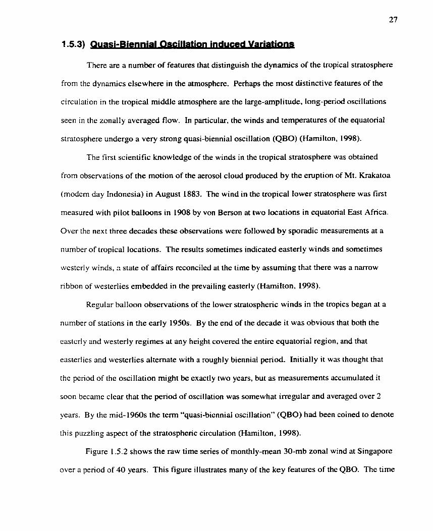
Figure 1 S.2 shows the raw time senes of monthly-mean 30-mb zona1 wind at Singapore
over a penod of 40 years. This figure illustrates many of the key features of the QBO. The time

series is clearly dominated by an alternation between easterly and westedy wind r e m
roughly every 2 to 3 years. The extrem in the prevaïJing winds very h m cycle to cycle, but
the peak easterly (20 to 25 mls) always exceeds the peak westcdy winch (10 to 17 d s ) .
According to Hamilton (1998). the timc series has a rough square-wave character with rapid
transitions (-2-4 months) between pcriods of fairly constant prevailing easteriies or westedies.
Figure 152: 'Rme strks of tbt montbly-mean zonil wiaâ (Smb) - r d at SiiiprMre (13N) d o h g the period 1 W to t000. This dimgmm dawrrs tm the cquirtortrl QBO.
The quasi-bienniai wind reversais invariably appear first at high levels and then descend.
At any level the transition be-n easterly and westeriy regimes is rapid so that the transitions
are also associated with strong vertical shear. Much of the variability in the period of QBO is
associated with the changes in the length of the easterly phase. particularly above about 50-mb.
nie maximum amplitude occurs near 30-mb and the amplitude b p s off to srnall. but
apparently stiil detectable values near the tropopause (-1 7 km). The drop off in QBO amplitude

above 30-mb is very gradua1 and the oscillation is still very strong at the 10-mb level. At almost
al1 times the easterly to westerly transitions are more rapid than vice versa, and the associated
westerly shear zones are considerably more intense than the easterly shear zones. Among the
complications in determining the details of the QBO signal is the fact that the annual cycle
becornes strong off the equator and itself has considerable geographical variability. A QBO in
temperature has also been observed with peak amplitude of -2-3°C (Hamilton, 1998 and
references therein).
Variations of total ozone are highly correlated with ozone variations in the lower and
middle stratosphere where the ozone photochernical relaxation time varies from one to several
months. It is therefore to Se expected that transport processes play a major role in producing the
ozone oscillations. When the observed variations in the tropics are filtered for annual and
semiannual periodicities and long-term trends, the residual variation shows a strong relationship
to the QBO of the zonal tropical wind in the stratosphere such that maximum ozone is
associated with strong West winds. Observations also indicate that at the equator the QBO in
ozone is positively correlated with the QBO in temperature at 50-mb (i-e., maximum ozone
occurs with maximum temperature) (London, 1985 and references therein). The basic
explanation of the ozone QBO was provided by Reed (L965), who noted that the changes in the
temperature in the QBO should be connected with a QBO in the diabatically-induced meridional
circulation. The anomalous rising and sinking motion associated with the QBO temperature
changes cause variations in any trace constituent with a mean vertical stratification. If there is
also a strong vertical gradient in the chemical lifetime of the constituent, then it is possible to
produce a QBO in the integrated total column concentration. For the case of ozone, the mixing
ratio increases rapidly with height in the lower and rniddle stratosphere and the chemical
tirnescales decrease rapidly with height. As the QBO westerlies descend, the anomalous mean
meridional sinking depresses the ozone isopleths near the equator. Since the chernical timescale
is short at high levels, the ozone that is pulled down from the middle stratosphere is replaced
rapidly, while at lower latitudes the ozone acts more nearly as a passive tracer. Thus the descent
is associated with an increase in the total ozone column, and the equatorial ozone column
reaches its maximum value after the westerly shear zone has descended through most of the
stratosphere (Harni Iton, 1998).
The phenornenon of equatorial QBO is well known. What is not well known, but
increasingly becoming apparent observationally, is that a QBO signal ako exists in the
extratropical stratosphere in dynamical variables and tracer fields: water vapor and column
ozone. There is as yet no generally accepted explanation of how the equatorial QI30 anomaly is
transmitted to the high latitudes, where, at least in the case of column ozone, the signal is
actually stronger than in the equatorial region (Tung and Yang, 1994).
Kinnersley and Tlrng (1999). however, proposed four mechanisms that would potentially
produce an extratropid QBO signai in ozone. These mechanisms are as follows.
Modulation of extratropical planetary waves (and hence the mendional circuIation) by
interaction with the equatorial zona1 wind QBO. Evidence for such a modulation has
been obtained from observations.
Poleward advection and/or diffusion of the subtropicai ozone anomaly to middle and
high latitudes.
Advection by the direct QBO circulation. An interaction of the equatorial QBO with the
seasonal mean circulation may result in a strongly seasonal QBO circulation anomaly
extending into subtropical and perhaps middle latitudes in the winter hemisphere.

Modulation of the photochetnical equilibriurn value for ozone above about 25 km due to
the anomaious advection of other trace gases, in paticular NO2. (Kinnersley and Tung,
1999).
1.5.4) El Nino-iauced VBCLBuQaS .- . . .
The El Nino oscilIation is characterized by anomalous sea surface temperatures
occumng at intervals of between two and seven years, the average period k ing forty months.
These alter the tropical oceanic circulation patterns, particularly in the Pacific. It is known to
have global repercussions for atmospheric circulation and climate (William and Toumi, 1999).
Total column ozone observations (for example: Zerefos et al., 1992; Shiotani, 1992;
Randel and Cobb, 1994 as referenced by William and Tourni, 1999) have suggested a srna11 but
significant four to five year signal in ozone arnount that has been Iinked to the El Nino/Southern
Oscillation. This takes the form of a decrease in tropical total ozone, with increases occuning at
extra-tropical latitudes. This connection between ozone and the changes in sea-surface
temperature occuning during El Nino has been attributed to a direct linking mechanism between
ozone distribution and surface temperature. Through this mechanism, an increase in surface
temperature such as that seen in the tropical western pacific during El Nino leads to changed
ozone in two ways. First, through increased evaporation activating cumulus convection and
thus i ncreasi ng tropopause altitude and, second, through an enhancement of the Brewer-Dobson
circulation. Each of these will result in tropical ozone decrease for the El Nino surface
temperature enhancement, with an increase in the extra-tropics (William and Toumi, 1999 and
re ferences therein).

1.6) TRENDS IN TOTAL OZONE
Since the rnid-1980s substantial changes in the ozone layer have k e n detected. The
discovery of the ozone hole in Antarctica was the first unequivocal evidence of stratospheric
ozone depletion. At that time total ozone levels in spring over Antarctica had dropped to 200
DU from the 30-350 DU levels prevâiling in the 1960s and 1970s. Since that time, the hole
has become, in general, deeper and wider each year. In the 1990s minimum ozone values of
1 10-1 20 DU were seen in Antarctica almost every year, and the totd area with spring ozone
vatues beiow 220 DU exceeded 20 million km'. Total ozone values less than 100 DU were
rneasured in both 1993 and 1994, with the record low value of 88 DU measured on September
28, 1993. In 1996 a minimum ozone value of 11 1 DU was recorded, while the area of the hole
was almost as large as in the peak year of 1993. Ozonesonde data have shown total destruction
(>99%) of ozone from 14 to 19 km (i-e., the lower part of the ozone layer) during ozone hole
episodes in recent years (Environment Canada, 1999 and references therein).
Ozone decline over midlatitudes have also been observed but is generally much weaker
than in the Antarctic, although it can be clearly seen from the long-term data records. In the
equatorid belt there are no significant ozone changes, although a temporary 2-3% total ozone
decline was evident after the Mount Pinatubo eruption (Environment Canada, 1999 and
references therein).
Ozone losses in the Arctic are generally smaller than in the Antarctic: typically about
12% in the winter-spring column ozone. This difference is known to be associated with the
differences between the Arctic stratospheric vortex and the Antarctic stratospheric vortex. In
the Antarctic, the vortex and the cold temperatures within it persist longer into spring than is the
case with the less circular and generally weaker and warmer Arctic vortex. The combination of

low temperature (c-80°C) and sunlight, which allows rapid destruction of ozone, oçcurs to a
much greater extent in Antarctica than in the Arctic (Environment Canada, 1999).
The greatest uncertainties in the present understanding of observed ozone changes have
to do with the cause of midlatitude ozone reduction. There are many ways in which dynamical
and chernical processes can be expected to be relevant. Sections 1.6.1 to 1.6.6 will provide an
overview of the proposed mechanisms potentially responsible for rnidlatitude ozone changes.
1.6.1) The Role of Heteroaeneous Chemistrv on MiQLgfjfyde 0-
Statistically significant decreases in total ozone were first observed in Antarctica, but are
now well documented over much of the globe. While direct observations of chlorine monoxide
(CIO) and related chernical compounds have confirmed the predominant role of anthropogenic
chlorinated and brominated hydrocarbons in causing the decline of Antarctic ozone, the reasons
for midlatitude ozone trends have k e n much harder to establish. Observations of the ozone
profi le have shown that much of the observed column decrease has occurred in the lower
stratosphere at midlatitudes (below about 25 km), but present models under-predict the observed
decreases at those key altitudes (Solomon et al., 1996 and references therein).
Numerical mode1 simulations suggest that chemical processes assoçiated with sulfate
aerosol chemistry should decrease midlatitude ozone abundances after major volcanic eruptions.
Support for a volcanic impact on ozone has corne from observations of changes not only of
ozone but also of related chemical species such as NO2 and HN03 following the very major
eruption of Mt. Pinatubo in 1991. Measurements of the ozone profile and column revealed
record low ozone amounts at midlatitudes in the northem hemisphere after Pinatubo. In
addition to the Iarge but transient enhancements in sulfate aerosols caused by major volcanic
eruptions, there is evidence of an increase in northern hemisphere stratospheric aerosol

abundances over the past several decades. It is not clear whether this change is due to the
lingering effects of multiple volcanic events or to other sources such as carbonyl sulfide (OCS)
sulfur emissions from high-flying subsonic aircrafts. Nevertheless, direct observations by
independent techniques have established that Northern Hemisphere stratosphenc sulfate aerosol
abundances have increased over decadal timescdes- Modeling studies have shown that
inclusion of the heterogeneous chemistry associated with sulfate aerosols can significantly
increase the calculated trends in stratospheric ozone due to an increase in the abundance of
chlorine and bromine compared to gas phase mode1 calculations (appendix B, section 6.1 and
6.1) (Solomon et al., 1996 and references therein).
Much of the sarne sulfate aerosol chemistry presented in appendix (B) for polar latitudes,
can also dominate in mid latitudes. Narnely, two important heterogeneous reactions occumng
on sulfate aerosols at midlatitudes in the Iower stratosphere are:
. &O5 + HzO (a) 2HN03 (1 -6.1) BrONOz + H20 (a) + HOBr + HN03 (1.6.2)
These hydrolysis reactions are important since they change the relative balance between active
and reservoir species. Reaction 1.6.1 decreases the abundance of reactive nitrogen in the
stratosphere, but increases those of reactive chlorine (CIO) and to a lesser extent, hydrogen
(HO,) radicals which destroy ozone in the lower stratosphere. Thus, an increase in the rate of
heterogeneous reaction 1.6.1 results in an enhancement of ozone abundance in the middle
stratosphere (where its loss is dominated by NO,) and a reduction of ozone abundance in the
lower stratosphere (where CIO, and HO, radicals play a dominant role in its destruction)
(Solomon et al., 1996 and Tie and Brasseur, 1995). The net effect on ozone depends upon the
balance between these effects, but in the lower stratosphere (below about 20 km or so), this
process accelerates the net ozone loss for current levels of total chlorine (Solomon et al, 1996).

Active chlorine species will increase because the reduction in NOz will result in less CIO k ing
present as CIONO7, a chlorine reservoir species (Chartrand et al., 1999). The rate of reaction:
is also reduced, and hence the destruction rate of ozone by chlorine is enhanced (Granier and
Brasseur, 1992).
Reaction 1.6.2 is a significant source of HO, in the lower stratosphere and thereby
represents a mechanism for linking bromine trends to ozone depletion and aerosols (Solomon et
al., 1996). Through this mechanism, odd hydrogen will increase due to the photolysis of HOBr
and HNO; via:
HOBr + lzv --+ OH + Br (1 -6.4) HN03 + hv --+ OH + NO2 (1.6.5)
L
The enhanced OH and HOz will increase ozone destruction through the HOs catalytic cycles:
0 H + 0 3 + H O z + 0 2 (1.6.6) HO2 + 0 3 + OH + 202 (1.6.7) Net: S 0 3 + 302 (1.6.8) H + 0 3 + O H + 0 2 (1.6.9) 0 H + O + H + 0 2 (1 -6.10) Net: O + O3 -, 202 (1.6.1 1)
In addition, the increased OH will also release CI from HCI, another reservoir species through
the following reaction:
I OH + HCI + Cl + H20 ( 1 6 . 2 ) 1 Reaction 1.6.12 also results in increased CIO levels (Chartrand et al., 1999).
Like the polar stratospheric clouds that enhance Antarctic ozone depletion compared to
gas phase chemistry, liquid aerosol enhancements increase the efficiency of halogen chemistry
for ozone Ioss at midlatitudes but are not a mechanism in themselves for substantial ozone loss
independent of human inputs of chlorine and bromine to the stratosphere. It is well known that
current photochernical models simulate reasonably well the ozone losses observed above 30 km
or so at midlatitudes but fait to capture the ozone depletion observed at lower altitudes (and
hence underestimate the total column loss). The explicit considention of aerosol content is a
substantial factor in deterrnining the shape of the profile of ozone depletion below about 30 km,
and while according to mode1 simulations it does not account for al1 of the observed ozone
depletion in midlatitudes, it certainly plays a key role in the rate of obsewed midlatitude ozone
depletion through the combination of reactions shown above (Solomon et al., 1996).
1.6.2) The Role of Cirrus Clqyds O-e Ozone D e ~ l e t i a
Cloud formation depends upon temperature and the availability of condensable vapors.
In spite of the extreme dryness of stratospheric air, clouds occur from about 15 to 26 km above
the polar regions due to very low ternperatures. While the tropopause region at sub polar
latitudes is considerably warmer than the polar stratosphere, it can be quite humid, allowing the
formation of c ims clouds (Solomon et al., 1997 and references therein). In studies done by
Bornnann et al. (1996, 1997) (as cited by Solomon et al., 1997), it was shown that cirrus clouds
near the tropopause in midlatitudes might lead to chemical reactions similar to those of water-
ice polar stratospheric clouds. Bonmann et al. (1996, 1997) suggested that these clouds could
affect the abundances of key radicals such as Cl0 near the midlatitude tropopause and thereby
perturb the local chemistry, leading tu ozone depletion (Solomon et al., 1997).
AI1 satellite studies have revealed frequent c ims clouds near the tropopause in the
tropics. High-altitude cirrus clouds were also observed, albeit less often in the midlatitudes.
However, there is evidence that cirrus clouds can occur not only in purely tropospheric air near
the tropopause, but also in air with a chemical composition reflecting a stratospheric
contribution, particularly at the interfaces between stratosphenc and tropospheric air (Solomon
et al.. 1997). To examine the chemical perturbations which could be caused by cirrus clouds in
the vicinity of the tropopause, and to provide an estimate of their possible impact on ozone
trends in this region, Solomon et al. (1 997) used a two dimensional
chemical/dynamica~radiative model to evaluate chemical processes relating to c i m s cloud
occurrences for typical air parcets.
According to SoIomon et al. (1997), observations of ozone and limited measurements of
HCI suggest that Cl, abundances near the tropopause are of the order of LOO pptv, with larger
amounts being present at higher latitudes. Any CIONOz andor HOC1 present in the tropopause
region is highly likely to rapidly react with HCI on c ims cloud surfaces, suggesting that CIO
abundances could increase from pptv or sub-pptv levels near the tropopause to considerably
larger values due to cirrus cloud chernistry. The magnitude and duration of such perturbations
depend upon season, altitude, and latitude. Hydrogen radical concentrations are also affected by
c ims cloud chemistry involving chlorine species, providing an additional perturbation and an
indirect mechanisrn that likely influences ozone loss. Nitrogen radical concentrations are
expected to be reduced by cirnis cloud chemistry. The relaxation of active chlorine to HCI is
expected to occur rather slowly in the lowerrnost stratosphere at middIe and high latitudes, over
timescales of days or weeks depending upon season and latitude. Hence CIO enhanced by cirrus
ciouds may persist long after a cloud has dissipared. The peak-calculated enhancements in CIO,
due to the presence of cirrus clouds, in the midlatitudes near the tropopause are of the order of
factor of 30 (Solomon et al., 1997).
Given the large ozone depletions observed in the vicinity of the midlatitude tropopause
particularly in clean environments such as over western Canada, any perturbation to Cl0 in this
region is of considerable scientific interest, albeit that the presence of cirrus clouds near the
tropopause, according to the Solomon et al. (1997) model study, plays only a small role in

deterrnining the total ozone column trends, i.e. 1 to 1.5% change in computed column at
midlatitudes (Solomon et al., 1997).
In short, the modeling results presented by Solomon et al. (1997) suggest that the
sudaces of cirrus clouds near the tropopause likely provide sites for activation of chlorine (and
perturbations to related species such as NO, and HO,), much as polar stratospheric clouds do at
higher altitudes over polar-regions and for sirnilar reasons. Their results suggest that
consideration of cirrus cloud chemistry at rnidlatitudes may make important contributions to the
shape of the ozone depletion profile in the lower-most stratosphere, which couId play a role in
reconciling discrepancies between observed and modeled ozone depletion at midlatitudes
(SoIomon et al., 1997), and partial1 y expfain high rates of total column ozone reduction
obsewed in midlatitudes.
1.6.3) The Possible Role of IoQine on Ozone De~letioq
The possible role of iodine ,/I) in rnidlatitude stratospheric ozone depletion has k e n
examined using a 2-D chemical transport mode1 (Solomon et al., 1994). CFCs have long
chemical lifetimes of many decades or more and essentially al1 CFCs emitted at the surface
ultimately reach the stratosphere, but the chlorine they contain only becomes readily available
for free radical chemistry at high altitudes or in the polar regions where air descends from high
altitudes and encounters an unusual chemical environment capable of releasing radicals from the
reservoirs. Iodocarbons are quite different in that the bonds involving iodine are generall y very
weak and photochemically active, leading to the rapid release of active iodine from source gases
and reservoirs as well as yielding very short troposphenc lifetimes of only a few days or weeks
for iodine source gases, which could limit the arnount of iodine that can reach the stratosphere
(Solomon et al., 1994).

It has generally been assumed that the short tropospheric Iifetimes of iodocarbons would
preclude significant transport of these gases to the stratosphere (i-e., the source gases would
decompose and their products rain out befoe reaching stratosphenc altitudes) (Solomon et al..
1994). However, recent studies have shown that convective clouds can transport insoluble
materials rapidl y from low altitudes to the upper troposphere and lower stratosphere (Gidel,
1983; Chatfield and Crutzen, 1984; Pickering et al., 1992; Kritz et al., 1993; Danielsen, 1993:
as cited by Solomon et al., 1994).
Biogenic processes in the oceans represent a substantial source of iodine to the lower
atmosphere. Methyl iodide is believed to be produced by marine phytoplankton and other
sources such as kelp and perhaps macroalgae, and there is evidence that biogenic sources of
chloroiodomethane and other iodocarbons may also be substantial. Changes in ocean
temperature (perhaps caused by El NiRo, see Section 1.5.4) or other factors could potentially
yield trends in emissions of these compounds (Solomon et a!., 1994). The globally averaged
Iifetime for metliyl iodide is calculated by Solomon et al. (1994) to be 4 days with a timescale
for photochemical loss throughout the tropical troposphere that exceeds 2.5 days (Solomon et
al., 1994).
According to various studies (Singh et al., 1983; Rasmussen et al., 1982; Reifenhauser
and Heumann, 1992; Atlas et al., 1993; as cited by Solomon et al., 1994), the abundance of
methyl iodide in the whoIe atmosphere ranges from 1 to 10 parts per trillion by volume (pptv).
Observations suggest a global oceanic source of iodine from methyl iodide ranging from a
minimum of 0.3 to as much as 3 T&r. Industrial sources of iodocarbons appear to be
negligible compared to oceanic sources, however iodocarbons generated by biomass buming
could contribute to the iodine reaching the stratosphere. Biomass buming is a key source of
man y important atmosphenc gases, includi ng methyl chloride and meth y1 bromide. Since the

elemental abundance of iodine in plant matter is comparable to, or greater than that of bromine,
it is highly likely that methyl iodide is also produced in this fashion; compounds such as
chloroiodomethane and bromoiodomethane are also possible products. On the whole, the total
iodine abundance of the stratosphere could be as large as O. 1 to 3 pptv and there could have
been some trend in abundance due to increased biomass burning or changes in oceanic
conditions (Solomon et al., 1994).
Solomon et al. (1994) has suggested that like Cl0 and BrO, ozone depleting interhalogen
reactions could lead to rapid ozone Ioss. Examples of such catalytic cycles involving chlonne
and bromine are:
The net reaction represented by each of these catalytic chahs is 2 0 3 + 302, which can be
effective in the lower stratosphere. The efficiency of iodine released in the stratosphere for
ozone destruction near 15 to 20 km altitude, as represented by the above reactions, is more than
1000 times greater than that of chlorine, and thus even very small amounts of iodine couid cause
significant ozone destruction (Solornon et al., 1994). The results from the Solomon et al. (1994)
study based on the 2D chemical transport mode1 however, illustrates that the presence of iodine
or a trend therein is not sufficient on its own to produce substantial ozone loss. Only in
combination with trends in chlorine and bromine are total ozone losses calculated in excess of
1%. Thus like the polar stratospheric clouds that play a role in polar chemistry, iodineTs role in
ozone depletion is highly likely to be pnmarily one of enhancing the ozone depletion due to
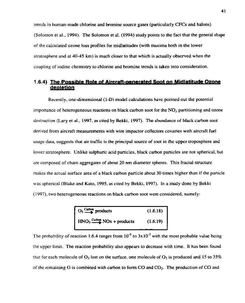
trends in human-made chlorine and bromine source gases (particularl y CFCs and halons)
(SoIomon et al., 1994). The Solomon et al. (1994) study points to the fact that the general shape
of the calculated ozone loss profiles for midlatitudes (with maxima both in the lower
stratosphere and at 40-45 km) is much closer to that which is actually observed when the
coupling of iodine chemistry to chlorine and bromine trends is taken into consideration.
1.6.4) The Possible Role of Aircra I aeneraed Soot on -de Ozong
Recently, one-dimensional (1-D) mode1 calculations have pointed out the potential
importance of heterogeneoiis reactions on black carbon soot for the NO, partitioning and ozone
destruction (Lary et al., 1997, as cited by Be&, 1997). The abundance of black carbon soot
derived frorn aircraft measurements with wire impactor collectors covaries with aircraft fuel
usase data, suggests that air traffic is the principal source of soot in the upper troposphere and
lower stratosphere. Unlike sulphuric acid particles, black carbon particles are not spherical, but
are composed of chain aggregates of about 20 nm diameter spheres. This fractal structure
makes the actual surface area of a black carbon particle about 30 times higher than if the particle
was sphencal (Blake 2nd Kato, 1995, as cited by Bekki, 1997). In a study done by Bekki
(1997), two heterogeneous reactions on black carbon soot were considered, namely:
CIrboa 0 3 + P ~ U C ~ S (1 .6.18)
cartJO0 HN03 + NOx + products (1 .6.19)
The probability of reaction 1.6.4 ranges from L O - ~ to 3x10-' with the rnost probable value being
the upper limit. The reaction probability also appears to decrease with time. It has been found
that for each molecule of O3 lost on the surface, one molecule of Or is produced and 15 to 35%
of the remaining O is combined wi th carbon to form CO and COz. The production of CO and

CO- implies a possible loss of carbon during the reaction. The fate of the rest of the odd oxygen
is unclear. When the odd oxygen is not regenerated, reaction 1-6-18 is a straightforward ozone
destroying mechanism. Unlike the usual chernical cycles of ozone destruction, the efficiency of
this mechanism does not depend on the presence of sunlight or the concentration of a particular
radical (Bekki, 1997).
The reaction probability of equation 1.6.19 ranges from 0.02 to 0.04. The products of
this reaction could be HzO and NO, with five times more NO2 produced than NO. This reaction
is a renoxification mechanisrn which could counteract the denoxification effect of
heterogeneous chemistry on sulphunc acid aerosols (Bekki, 1997).
Bekki (1997) used a fully interactive 2-D radiative-convective-photochernical modef,
incorporating reactions 1.6.18 and 1.6.19, extending from pole to pole and from the surface to
around 95 km with a resolution of 3.5 km vertically and 9-5" horizontally. The model ran from
1974 to 1992 and perforrned 4 separate runs. The first run included the aircraft ernissions of
HîO, NO,, and SO,, but not of black carbon. The second run included al1 the components of
aircraft emissions along with a reaction probability of 10" for reaction 1-6-18. The third run
was very similar to the second run, but the reaction probabili ty for reaction 1.6.18 was set to
2 x IO-'. The final run included al1 the cornponents of aircraft emissions along with a reaction
probabili ty of 0.028 for reaction 1.6.19. Although the ozone trends calculated by this 2-D
mode1 are subject to a number of uncertainties i.e. the results are sensitive to the assumed O;
uptake rate on soot which is uncertain (for a complete discussion of uncertainties refer to Bekki,
1997). by accounting for the catalytic heterogeneous reduction of O; on aircraft-generated soot,
the model was able to reproduce a large part of the lower stratospheric ozone trend observed at
Nonhem Hemisphere middle latitudes (Bekki, 1997).

Measurements of HCI, CIONOz and CI0 in both the Antarctic and Arctic support the
view that heterogeneous chernical reactions on the surface of polar stratospheric clouds (PSCs)
release reactive chlorine species from the reservoir species HC: and CION02, leading to large
CIO enhancements. The measurements indicate that the regions of perturbed chemistry are
largely confined to the polar vortex. The impact of such processes on the stratosphere outside
the polar vortex is in question @ougiass et al., 1991).
According to Jones and Mackenzie (1995) however, polar-regions can affect the lower
latitudes in a number of ways. First, as the polar vortex breaks down in early spring, air within
the polar vortex, in which ozone may have ken depleted, is mixed with low latitude air,
reducing midlatitude ozone arnounts purely by dilution. If the vortex remains essentially intact
throughout the winter months, the maximum extent to which the vortex can contribute to
midlatitude ozone loss is determined by the amount of ozone within the polar vortex as it forms
in early winter. If however, the polar vortex is not well contained throughout the winter months,
processing (the passage of a substantial volume of high latitude air to midlatitudes) will occur
(Jones and Mackenzie, 1995 and references therein).
If vortex temperatures are cold enough, polar stratospheric clouds form, reactive chlorine
concentrations rise as a result of reactions on PSCs, and the sedimentation of PSCs causes
dehydration and denitrification. Denitrification allows active chlonne compound concentrations
to persist for longer period of time, thus promoting ozone loss. The passage of this chemically
processed air to low latitudes can thus increase ozone loss in that area. In such a situation,
although midlatitude temperatures rnay never have reached the threshold for PSC formation, the
effects of PSC chemistry would still be apparent. Midlatitude ozone loss, initiated by the

transition through the cold polar region, could then proceed (Jones et al., 1995 and references
therein).
Randel and Wu (1995) analyzed total global ozone measurernents from the Nimbus 7
total ozone mapping spectrometer (TOMS) using potential vorticity (PV) as an approximate
vortex-following coordinate, for a period of thirteen years, from 1978 to 199 1. They concluded
that the midlatitude ozone losses occur, not due to ozone depletion inside the vortex and
transport of ozone depIeted air (but rich in CIO) to midlatitudes (pure dilution), but it occurs due
to in situ rnidlatitude processes, possibly associated with vortex processed air transported to
midlatitudes or reactions associated with background sulfate aerosols (Randel and Wu, 1995).
In summary, recent studies using a range of mode1 types generally suggest that the
outflow of air from polar vortices into rnidlatitude stratosphere, while not zero, is small,
contributing at most several tens of percent to rnidlatitude ozone depletior.. The study of
Randall and Wu (1995) also supports limited outflow. However, a number of observational
studies (Proffitt et al., 1990, 1993; Tuck et al., 1992, 1993, 1994; as cited by Jones and
~Mackenzie, 1995) appear to be in conflict with this view, implying a much larger outflow, either
quasi-isentropically or by descent through the lower boundary of the vortex (Jones and
Mackenzie, 1995 and references therein). Regardless, the contribution of this mechanism to
rnidlatitude ozone depletion is not well understood presently, and further observational and
modeling research is still required.

Statistical studies of both radiosonde and satellite radiance data have demonstrated that
total ozone trends in both hemispheres are accompanied by lower stratosphenc cooling trends.
Although several one-dimensionai radiative model calculations, as well as three-dimensional
general circulation model studies have al1 concluded that the observed zonally averaged cooling
trends in the northern winter could, in principal, be explained as primarily a radiative response
to the observed ozone trends, Hood et al. (1997) suggest that at Ieast part of the observed lower
stratosphenc cooling trends could also be a consequence of dynamical heating changes if a
major part of the NH midlatitude ozone trend is a result of dynamical transport effects.
Generally, transport-induced temporal changes in total ozone in the M-I are accompanied by
positively correlated changes in lower stratosphenc temperature and negatively correlated
changes in geopotential height. During the period when lower stratospheric cooling trends were
observed at NH winter midlatitudes, positive height trends were also observed (Hood et al.,
1997 and references therein).
The role of dynamics in observed ozone and temperature trends has been investigated on
a regional scale by Fortuin and Keider (1996, as cited by Hocd at al., 1997). Their analysis of
concurrent ozone and temperature soundings over the t 983-1993 period indicates that, at 4S0N
and 1 1°W, the observed lower stratospheric ozone and temperature trends are both consistent
with a long-tem increase in the average vertical velocity component in winter (i.e., more
upwelling). Therefore, it is plausible to consider the hypothesis in which al1 or part of the
observed NH midlatitude cooling trends reflect long-term differences in lower stratospheric
circulation that has in turn accelerated the effective reduction of total ozone at midlatitudes
(Hood et al., 1997).

According to Hood et ai. (1997), an early observation that "shed light on" the possible
importance of their hypothesis was the existence of a significant longitude dependence for
TOMS total ozone trends, oiiginally noted by Stoiarski et al. (1992). In 1994, Randel and Cobb
demonstrated that similar geographic dependence could also be found for trends derived
statistically from microwave sounding unit (NISU) channel4 temperature data for the lower
stratosphere (50 to 150 hPa). They further indicated that both ozone and temperature trends
resembled a zonal wave 1 pattern, which suggests a dynamical origin for this spatial dependence
(Hood et al, 1997). Hood and Zaff (1995), using a perturbation ozone transport model, found
that the zonally asymmetric component of the observed total ozone trend in January can be
quantitatively simulated using observed changes in the structures of quasi-stationary waves in
the geopotential height field between the early 1980s and the late 1980s. They also noted that
seographic distri bution of 100 hPa geopotential height anomalies between the earl y and late
1980s is inversely correlated with the geographic distribution of total ozone trends (Hood et al.,
r 997).
On seasonal and longer timescales, the zonal mean ozone and temperature distributions
in the lower stratosphere are determined by a balance between net radiative heating and cooling,
photochernical production and loss, and meridional transport of heat and chemical species by
eddy motions. In winter, these eddy motions consist primarily of quasi-stationary planetary
(Rossby) waves. Thus temperatures and long-lived trace constituents such as ozone are strongi y
influenced by disturbances that propagate upward from the troposphere. The local convergence
of eddy heat and momentum fluxes combine to exert a zonai mean force per unit mass on the
background zonal flow, inducing a mean mendional circulation which transports ozone-rich air
from the tropical stratosphere poleward and downward to the extratropics (Hood et al, 1997 and
references therein).

Given prescribed values of the wave driving, the observed temperature distribution, and
an accurate radiative transfer scheme, it is possible, in principle, to perform a diagnostic
calculation of the meridional circulation. In practice however, calculation of the wave forcing
from observations is problematic due to the limited spatial resolution of available data sets and
the highly derived nature of the quantities to be calculated (Hood et al., 1997, and references
therein). However, given the limitations of available long-term rneteorological data sets for the
upper troposphere and lower stratosphere, Hood et al. (1997) developed an empirical approach
toward estimating long-term ozone variability resulting solely from differences in ozone
advective transport as reflected in 100 hPa temperature and height fields. While their empirical
approach does not represent an absolute calculation of the dynamical contribution to total ozone
trends, their results suggest that differences in advective transport of ozone can account for a
significant fraction of zonai mean midlatitude trends (Hood et al., 1997).
As rnentioned earlier, the possil'ility that some part of the long-term 100-hPa
temperature decline represents a direct radiative response to the observed ozone decline cannot
be eliminated. If so, this would have the effect of inflating the estimates for the dynamical
contribution to ozone trends. However, according to the empirical approach used by Hood et al.
(1997), at 45' N, the observed 100-hPa temperature variation is accompanied by 100 hPa height
variations in the opposite sense on both short and long timescales. However, this characteristic
is not predicted by radiative model calculations and suggests a role for dynarnical variability in
producing 100 hPa temperature trends (Hood et ai., 1997).
A related question is the origin of the long-term dynamical changes that apparently
contribute substantially to midlatitude ozone trends. Because of the shonness of the radiosonde
data record (less than J O years), it is not possible to determine empirically whether the observed
trends in the lower stratospheric geopotential height and temperature are part of a long-term,

natural climatic oscillation or are an early manifestation of a long-terrn climatic trend such as
global warming. It has k e n suggested that a long-term greenhouse gas-related increase in
tropical tropospheric temperatures is responsible for lifting the geopotential height surfaces in
the Iower stratosphere at latitudes < 50" N. This results in an initial strengthening of the polar
vortex which inhibits poleward planetary wave propagation and cooIs the polar stratosphere in
Iate faIl and early winter. The polar cooling further strengthens the vortex in a positive feedback
loop (Hood et al., 1997 and references therein).
Most total ozone analyses and modeling studies focus either on global patterns or on the
individual Northern or Southern hemispheric patterns. The aim of this thesis is to analyze the
status of total column ozone concentration in a more regional context Le., over the whole North
American continent (Mexico, U.S., and Canada). More speci ficall y, the three main objectives
of this study are:
1. to examine the spatial and temporal variations of long term ozone concentration over the
North American continent,
2. to identify:
natural mechanisms responsibte for long term variations of total column ozone
concentration,
examine the relative importance of these natural mechanisms, and
further examine any spatial variations that may exist arnong these mechanisms, and
3. to determine the extent to which total column ozone data from a ground-based ozone
monitoring station is representative of the whole study area.

2.0) DATA SOURCES AND ANALYSlS METHOOS
A map showing the study area is given in Figure 2.0.1. Three separate data sets are used
in this study. They are:
Total Column Ozone data from Various Stations over North America,
Solar Sunspot Activity data,
and Singapore zona1 wind (QBO) data at 30-mb.
2.1 ) SOURCE OF DATA
2.1.1) Total Co- Ozone Rau
The total column ozone data used in this study were retneved from the World Ozone and
Ultraviolet Radiation Data Center (WOUDC). WOUDC is one of six recognized World Data
Centers, which are part of the World Meteorological Organization (WMO), Global Atmosphere
Watch (GAW) program. The WOUDC is operated by the Experimental Studies Division of the
Meteorological Service of Canada (MSC), formerly known as Atmospheric Environment
Services (AJ3)* Environment Canada located in Toronto.
The total column ozone data were retrieved from the World Ozone Data Center
(WODC) which is a sribsidiary of WOUDC. WODC operates a scientific archive and database
providing a variety of ozone data sets to the international scientific community. There are over
300 stations represented in the archive some of which comprise over 35 years of continuous
data. Data sets include total column ozone, surface ozone, vertical profile data from ozonesonde
f l ights, lidar measurements, and the Umkehr technique (WOUDC, 2000).

Figure 2.0.1: The study a r a (the siteilite is providai by mriprom, #100)
Ground-based total column ozone measurements are made using the Dobsoa-Brewer
spectrophotometers. Total column ozone data was reaieved h m 24 WODC stations (Table

The Solar Sunspot data used in this snidy was retrieved h m the Solar-Temesaial
P hysics Division of the National Geophysical Data Center (NGDC). The data retrieved h m
NGDC was the monthly mean relative solar sunspot numbers h m 1960 to 2 0 . This is a
continuous record that does not contain any months with missing data. .
2.1) situated throughout North Amena The data type used h m this archive is the daily Total
Column Ozone which represents the total thickne-ss o f the ozone layer in Dobson Units (DU).
Table 2.1: A summuy d WOUDC (htiiuir wed.
Station 1 N U ~ C I C--Y I p d ~ d I ~ ~ ~ ) I ~ a ~ a ~ i b u l r ! ( * w ) 65 104
105 r
106
Toronfo BcdfM
F a k b ~ b
Nashville 155 1 W h i h t S d ~
CAN USA
USA USA
1 ~ # ) 0 0 1963-19'71 1964-1972 1993-1998 1962- 1998 1972-198 L.
18 19 192 199 20 21
, 217 22 24 241 290 3 19 320 321 338 51 64
76
77
1987-1995 1937-1998 1974-1996 1973-1998 1958-1998 1957-1997 1934-1992 1958-19'75 1957-1999 1988-1999 1990-1999 1993-1999 1992-1999 1992-1999 1994-1999 1957-1998 1962- 1967 1962- 1999 1964-1998
43.8 42.4
64.8
36.2
79.5 71.3
147.9
û6.6 324
AIat B i s e
M c ~ ~ w City Barrow Cariboci FdmMitni PdterFht Gmm Bay R ~ ~ ~ l u o e
Sa~katoon Sahma Island
Montnat WlllIUpe~
Halifàx Bratîsrakt(Rejgha)
Reykjavik S t d h ~
Goose Bay Chw~hill
106.5 82.5 46.8 19.3 71.3 46.9 53.5 65;l 44.5 74.7 521 48.8 45.5 49.9 44.7 50.2 64.1 39.0 53.3 58.7
CAN 1
USA MEX USA USA CAN USA USA CAN C M CAN CAN CAN CAN CAN ISL USA CAN CAN -
62.3 I
100.8 99.2 156.6 I
68.0 1
114.1 1475 88.1 I
95.0 106.7 123.1 73.8 I
97.2 63.7 104.7 21.9 77.5 60.3 94.1

2.1.3) QBO Dam
Monthl y mean zona1 wind data, from 1960 to 3000, measured over Singapore (at 30-mb)
was retneved from the Institute of Meteorology at the Free University of Berlin. This is also a
continuous data set that does not contain any months with missing data. In this data set,
negative values represent the easterly winds while the positive values represent the westerl y
winds.
2.2) STATISTICAL ANALYSIS
2.2.1) Qailv Total Colylnn Ozong
Monthly means were calculated from the daily total column ozone data for each station;
thus the subsequent analyses performed in this study are based on monthly mems of total
column ozone data. This step was necessary because the daily records obtained from each
station were not of equal length. Some montlis contained more daily measurements that others,
therefore, performing statistical analyses on the daiiy data would have resulted in biased results.
The ozone data from Station 65 (Toronto) has the most continuous record. Total column
ozone data from other stations often contained gaps of various lengths. In order to minimize
an y poten tial errors assoçiated wi th the subsequent statistical anaIyses performed in this study,
attempts have been made to minirnize the gaps in the following way: for each gap, the total
monthly ozone value is interpolated based on the monthly ozone values from three months
before and three months after. Each interpolated monthly ozone value was then examined to
make sure it follows the seasonal pattern based on the adjacent values, or else, it was ehminated
and was left blank.
In order to perform meaningful statistical analyses on monthly ozone data, attempts have
been made to minimize the seasonal variations. Several different methods have k e n examined

and the 13-month mnning mean method proved LO be the most effective. Section 3.3.1 provides
a detailed discussion of these methods, and the 13-month running mean method is used
throughout this study to minimize the seasonai cycles.
2.2.2) Time Series U a r R e m i o n Anglvsia
A simple time series and linear regression anaiysis was used to examine any possible
trends in total column ozone concentration over the study area. Although there are other forms
of regression analysis that can be used (Le., plynomial, teast squares, exponential, and etc.),
linear regression analysis is utilized because it is a standard method used in most ozone studies
to determine the long-term trend in total column ozone concentration. The slope obtained from
the equation of the line of best fit (i.e., the regression coefficient) detemines the long-term trend
in totaI column ozone concentration, and it is used to examine the spatial and temporal
variations in total colurnn ozone concentration that rnight exist over North America.
The significance of regression coefficient, also known as p-level, is also calculated and
is a primary source of information about the reliability of the linear regression analysis. More
technically, the value of the p-level represents a decreasing index of the reliability of a result.
The higher the p-level, the less reliable is the regression coefficient obtained through the linear
regession analysis (Statistica, 1995).
2.2.3) p e m ' s r Correlat ionvsis
The simple linear comelation coefficient (or Pearson's r) is used to evaiuate the extent to
which data from station 65 (Toronto), which has one of the longest and most continuous
records, i s representative of the whole of North America. This method is utilized because it is a
standard measure of correlation between two variables. It also does not require a determination

54
of whether a variable is dependent or independent, nor does it require the variable to be of the
sarne unit measurement (Statistica, 1995).
Pearson correlation assumes that the two variables are measured on at least interval
scales and i t determines the extent to which values of the two variables are proportional to each
other. Proportional rneans linearly related; that is, the correlation is high if a straight line can
summarize it. This Iine is called the regression line or least squares line, because it is
determined such that the sum of the squared distances of al1 the data points from the line is the
lowest possible (Statistica, 1995).
In a simple linear correlation, the resulting r value will fa11 between a range of -1.0 to
+1 .O. Negative values indicate an inverse relationship, positive values a positive relationship,
and a state of no correlation is indicated as r approaches zero.
If the correlation coefficient (r) is squared, then the resulting value (8, the coefficient of
determination) will represent thc proportion of cornmon variation in the two variables (Le., the
srrength or magnitude of the relationship) (Statistica, 1995). The simple linear correlation
coefficient r is calculated using the following equation:
(Clark and Hosking, 1986). The significance of correlation @-level) is also calculated and is a
pnmary source of information about the reliability of the correlation. As mentioned earlier, the
higher the p-level, the less reliable is the correlation coefficient obtained through the Pearson
correl ation anal ysis (Statistica, 1995).
55
2.2.4) S n e c t r u d Cross-Snectral Awvsis
Spectral analysis is concerned with the exploration of cyclical patterns in data. The
purpose of this analysis is to decompose a complex time series into a few underlying sinusoidal
(sine and cosine) functions of particular frequency. Pnor to spectral analysis, the series should
be detrended (so that it is stationary) and the mean should be subtracted from the series.
Otherwise, the density spectrum obtained will mostly be overwhelmed by a very large value for
the first cosine coefficient (for frequency 0.0). In a sense, the mean is a cycle of frequenc y zero
per unit time; that is, it is constant. Similarly, a trend is also of Iittle interest when one wants to
uncover the periodicities in the series. In fact, both of those potentially strong effects may mask
the more interesting periodicities in the data, and thus both the mean and the trend (linear)
should be removed from the series prior to analysis (Statistica, 1995).
Filtered seasonal time series and spectral analyses are used to illustrate longer than
seasonal time scale trends in the ozone data, and hence identify sources of natural total column
ozone variability, and their relative magnitudes, over the study area. A Tukey window with a
window width (also known as bandwidth) of 3 months is used to carry out the spectral analyses.
The Tukey window is a weighted moving average transformation, where for each frequency, the
weights (w) for the weighted moving average of the periodogarn values are computed as:
J w, = 0.5 + (O.Scos(lr - )) (for j = O to p), and P
I m-1 P Z - (m is the width of the moving average window). 2
While other spectral estimators such as Daniell, Parzen, Hamming, and Bartlett can also be
used, the Tukey window proved to be most effective in terms of exploring the cyclical patterns
in the total column ozone data. The objective is to find the frequencies with the greatest spectral

densities, that is, the frequency regions, consisting of many adjacent frequencies, which
contribute rnost to the overall periodic behavior of the series (Statistica, 1995). Spectral density
f, of a stationary time series xt, t = O, f 1, +2, . . ., at a certain frequency v, is calculated using the
following equations:
where R, (m) = E [ (x,,- p)(xt- p)] for m = 0, f l , 42, ... 0
and E is the expected value operator such that Et = k = Iedx
(Shumway, 1988).
Cross-spectral analysis is an extension of spectral analysis. The purpose is to uncover
the covariation between two series at different frequencies. The cospectral analysis is used in
this study in order to determine if QBO and sunspot data correlate with the total column ozone
data at the 2.5 and 11- year cycles, respectively. In other words, to determine whether or not the
periodicity in the QBO and sunspot data is synchronized with the total column ozone data.
A Tukey window with a window width of 5 months is used to cary out the cospectral
analyses. To test the significance of cospectral density peaks obtained through cospectral
analysis, both phase spectrum and squared coherence spectrum, also using a Tukey window
with a window width of 5 months, are computed. A cospectral density peak is significant only
if, at a given frequency, the phase spectmm is in phase (i.e., at or close to +2n radians) and the
amplitude of the squared coherency peak is also high. For example, if the amplitude of the
cospectral density peak is high, but the phase spectrum at that frequency is at O or close to zero
radians (i.e., out of phase), then the cospectral density peak at that frequency is not significant
even if the amplitude of the coherence spectrum is high. This means that the frequency
component of one series does not lead the other one; hence there is no causal mechanism
invoIved. Furthemore, if the amplitude of the cospectral density peak is hi&, and the phase
spectrum at that frequency is also at or close to e x radians, but the amplitude of the coherence
spectrurn, at that frequency is low, agiun even though there appears to be some causal
mechanism involved, the cospectral density peak is not significant. Only when the conditions
for both phase spectrum and squared coherence spectrum is met, the cospectral density peak, at
a gi ven frequency, is significant (Greenwood, 2000).

3.0) RESULTS AND DISCUSSION
3.1) ANALYSIS OF SECUUR TRENDS OF TOTAL OZONE OVER CANADA AND THE UNITED STATES
One of the primary objectives of this study is to confiml the existence of negative
secular trends in total ozone concentration over the study area and to further investigate the
spatial (both latitudinal and longitudinal) and temporai variations that may exist within this
region.
To investigate the latitudinal and longitudinal variations in total ozone concentration in
the study region, 10 stations were chosen that contained at least 20 years of total ozone
concentration data and covered geographically both east-west and nonh-south ends of the study
region. The stations chosen were divided into three transects, two !ongitudinal transects (one in
mid-Iatitudes-transect A, and one in high latitudes-transect B) and one latitudind transect
(transect-C) (Figure 3.1.1).
In order to investigate the presence, magnitude, and sign of any secular trends over the
study region, a ti me series and a linear regression analysis was performed on the monthly total
ozone concentration data available for each of the ten stations. The 13-month running mean
method was used to mitigate the seasonal variations in total ozone concentration from the data
and hence remove any outliers that might otherwise bias the results from the linear regression.

provided by map.com, Zûûû).
Figures 3.1.2 and 3.1.3 surnmarize the mc1~1t.s for uansects A and B which nin h m east to West
in the mid-latitudes and high-latitudes mpectively . Figure 3.1 -4 summarizes the cesults for
t ransec t4 which runs h m south to north in the mjddle of the study region. Table 3.1.1
further sumrnarizes the key feanires observeâ in figures 3.1.2 to 3.1.4, as well as providing

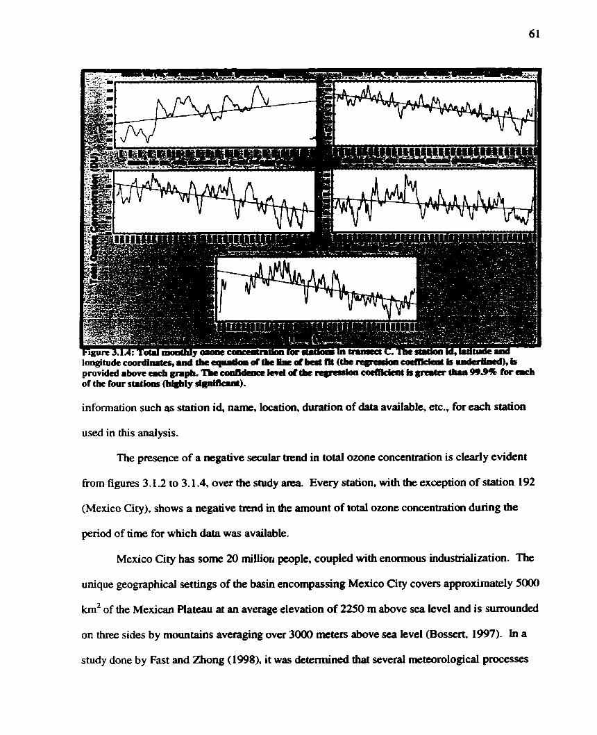
orovidcd above acô grrpâ. Tln caandeaot h d d ü œ cdfkkot b -ter thn 999% for acb or the tour strti- -1.
information such as station id, name. location, duration of data avaiiabfe, etc., for each station
used in this analysis.
The presence of a negative secular trend in total owne concentration is clearly evident
from figures 3.1.2 to 3.1.4. over the study area. Every station. with the exception of station 192
(Mexico City), shows a negative trend in the arnount of total ozone concentration during the
p e n d of time for which &ta was available.
Mexico City has some 20 million people. coupled with enormous indusnialization. The
unique geographical settings of the basin encompassing Mexico City covers approxirnately 5000
km2 of the Mexican Plateau at an average elevation of 2250 m above sea level and is sumwinded
on three sides by mountains averaging over 3000 meters above sea level (Bossect, 1997). in a
study done by Fast and Zhong (1998), it was detennined that several meteorological processes

Lltiûdnd -seet C 5om South to N d
are responsible for pollutant transport within the basin. One of these processes is called
"rnountain venting", or the "mountain-chimney effect" whereby pollutants are mixed upward by
means of vertical diffusion and vented into the free atmosphere (Fast and Zhong, 1998).
Tropospheric ozone is a pollutant and its concentration is relatively high over Mexico City.
Considering the high elevation and the unique geographical setting of Mexico City, along with
the meteorological process of mountain venting, it is possible that high concentrations of
tropospheric ozone are being entrained into the suatosphere over this area, and hence are
responsible for an increasing trend in the total ozone concentration observed aloft station 192
(fig. 3.1.4). Since there are no other stations available along the sarne latitude as station 192, it
is di fficuit to deterrnine whether the positive trend in total ozone concentration observed over
Mexico City is the nom for this latitude or otherwise.
Figure 3.1.2 shows the longitudinal variation in the trend of total ozone reduction dong
transect-A (mid-latitudes). Ail four stations lie within approximately the sarne latitude but
range from 68" W to 1 14" W. According to the siope of the regression line, the average
percentage of ozone reduction along transect-A, is approximately 6% per decade (table 3.1.1 ),
with the exception of station 65 (Toronto) which shows a slightly higher rate of total ozone
reduction per decade (7.68%). There is no apparent trend in the longitudinal variation of total
ozone reduction in mid-latitudes. The small variation that exists is probably random and
attributed to Iocalized conditions that can result in higher rates of ozone destruction in the
stratosphere. For example, Toronto has a higher population and is generally more industnalized
than Caribou, Bismark, and Edmonton. Hence, the rate of the emission of ozone destroying
radicals such as CFC's is greater over Toronto, than over the other three cities. Another
possibility is that the variations can be influenced by the location of the Rossby waves as
explained in Section 1.3.

Figure 3.1.3 shows the longitudinal vanation in the trend of total ozone reduction along
transect-B (high latitudes). The three stations lie within approximately the sanie latitude but
they range from 22" W to 157" W. The result of trend analysis for station 51 (Reykjavik) shows
a very minimum reduction in total ozone concentration that, when compared to other stations
along the same latitude (stations 24, and 199), does not follow the expected pattem in the trend
of total ozone reduction. According to Stolarski et al. (1992), the pattern observed from station
5 1 may reflect difficulty in measuring ozone at low Sun angles at this particular station. AIso, it
is important to note that the regression coefficient for station 5 1 has a very high p value (it's not
statistically significant). For these reasons, station 5 1 will be ignored when analyzing possible
trends in total ozone reduction along transect-B.
Although there appears to be slightly greater longitudinal variation in the trend of total
ozone reduciion in transect-B (as cornpared to transect-A) (table 3.1.1). there does not appear
to be any significant pattem to these variations. It is important to note that with respect to a
global scale, this is only a regional study spanning a relatively narrow range of longitudes. In
fact, global studies exhibit the presence of longitudinal variation in the rate of total ozone
depletion. According to Fusco and Salby (1999), total ozone is a highly variable property with
total column abundance changing loçally and daily by as much as 100%. Since the interannual
variability in ozone is caused by dynamic factors, such as the quasi-biennial oscillations (QBO),
El Nino-Southem Oscillations (ENSO) and Rossby waves, the ozone trends at different latitudes
Vary signi ficantly with longitude (Chandra et al., 1996). An anal ysis of Nimbus 7 TOMS data
extending from 1979 to 1990 perforrned by Niu et al. (1992, as cited by McCormack and Hood,
1997) revealed that iong-term trends in total ozone occumng in the Northem Hemisphere
exhibit significant longitude dependences at both middle and high latitudes. This is further
confirmed by Hood and Zaff (1995), where in studying the total ozone trends during 1980s, they

also discovered that in winter and earIy spring, distinct regions of significant negative trends
over eastern Russia and the eastern United States are separated by regions of smaIIer negative
trends, whiie slightly positive trends occur over the North Atlantic. Al1 these studies
demonstrate the presence of a significant longitudinal variability in total ozone trends, even
though this variability is not cleariy evident in our andysis.
Hood and Zaff (1995) suggested that chmges in the structure of the mean January total
ozone distribution in the 1980s could be reproduced quditatively from the observed changes in
the amplitude and phase of quasi-stationary planetary waves over the sanie period. They further
concl uded that decadal-scale variabili ty in the forcing of these disturbances in the troposphere
was primarily responsible for the observed longitude dependences of Northern Hemisphere's
total ozone trends in winter (this can be extended to other seasons as well). Further studies done
by Peters and Entzian (1996, as cited by McCormack and Hood, 1997) on the statistical
connection between variations in monthly mean values of geopotential height near the
tropopause and total ozone amounts lend support to the hypothesis that the geogaphical
dependences of total ozone trends are associated with dynamical anomalies originating in the
troposphere (McCormack and Hood, 1997).
With respect to latitudinal variation in the trend of total ozone reduction (transect-C) in
the study area, figure 3.1.4 (and aIso table 3. 1 -1) suggests that total ozone reduction increases
with Iatitude in the midlatitudes with a relative drop in the magnitude of the trend in the high-
latitudes. In fact, the rate of total column ozone reduction seems to be higher in Northem
rnidlatitudes than Northem high-latitudes. This pattern is further emphasized in figure 3.1.5
which shows both percentage of total ozone decline per decade and the absolute total column
ozone concentration as a function of latitude for the 10 stations used in the study region.
Absolute total column ozone concentration for each station was calculated by averaging al1 the

monthly total ozone concentrations for the total period of àata available. Agah, stations
representing hi&-latitudes (miàlatitudes) gcneraliy have higher (lower) concentrations of total
column ozone but demonstnitc ceiativdy lowa (highcr) rates of total column ozwc rcduction.
Whiie many snidies have achiowledged tbe existence of miciMitude total column ozone
reduction, none have made cornparisons between Northem rnidlatitude and high latitude rates of
total column ozone roduction (cornparisons arc oftcn made between the rates of Northtrn
micilatitude ozone reduction and Amairtic omne reduction). In this respect, our nnding is
unique.
As d i s c u s d carlier, many snidies using bath ground-based and satellite observation
have established chat total column ozone is decreasing in the middle and higher latitudes in the
northem hernisphere (Bojkov et al., 1990, 1994; Stolarskï et al., 1991, 1992; WMO, 1991, 1995;
de Winter-Sorkina, 1995, as cited by Hood et al., 1997). Negative mnds at high latitudes are

predominantly due to heterogeneous chemical losses on polar stratospheric cloud particles and
lower stratospheric aerosols, stenuning ultimately from anthropogenic emissions of
chlorofluorocarbons (WMO, 1991. as cited by Hood and Zaff, 1995). However, as was pointed
out in Section 1.6, the origin of midlatitude negative total trends (especially one that is greater
than higher latitudes) has not been completely established. Many different mechanisms are
proposed by different scientists to explain the unexpectedly large magnitudes of midlatitude
total column ozone reductions. Sections 1.6.1 to 1.6.6 provided a summary of some of these
mechanisms. For example, there are many ways in which dynmical processes can be expected
to be relevant. First, the height and structure of the midlatitude tropopause has a direct bearing
on total ozone abundance. Second, the strength of the Brewer-Dobson circulation controls the
transport of ozone from the tropical source region into the midlatitudes, and also controls the
rate of mean descent through the lowermost stratosphere into the upper troposphere. Third, the
transport of chemically processed air out of the wintertime vortex - either in a major vortex-
breaking event, such as a sudden warming, or in the final breakdown of the vortex - provides a
strong chemical perturbation in midlatitudes. The last example contains competing effects;
although breakdown and flushing out of the vortex ultimateIy limit ozone loss, there are short-
term losses in midhtitudes as PI-ocessed air reaches the lower latitudes and receives more
sudight. The extent of midlatitude ozone Ioss can be expected to depend on how rapid this
processed air gets diluted in the surf zone, which, like the vortex breakdown itself, depends on
the large-scale Bow (Environment Canada, 1999; and references therein).
In order to determine the cause of midlatitude ozone depietion, it is essential to quantify
the relative role of dynamical effects, chemical destruction, and the short-term impact of
aerosols from volcanic eruptions (which complicates the recent record). Purely advective
dynamical effccts (Section 1.6.6) should be capable of quantification, but others are far more
complex, for example, the impact of temperature changes on heterogeneous chemistry, the
impact of changes in the frequency of sudden warmings, or in the timing of the final vortex
breakdown. and on the propagation of polar ozone loss into midlatitudes. Such coupled
dynarnical-chernical processes are the most difficult to unravel (Environment Canada, 1999),
but indeed should be the focus of upcorning studies.
It should be noted that while mechanisms proposed in sections 1.6.1 to 1.6.6 can al1
coexist. thei r effects could dominate during di fferent seasons. For example, transport of ozone-
depleted air from the polar vortex could lead to large spring ozone depletion. Changes in
atmosphenc dynamics can affect ozone trends, but its effect is mostly maximized during winter.
While some fraction of ozone depletion produced earlier in the year could persist into the
summer season, the occurrence of a summer depletion maximum, is mostly attributed to local
photochemical losses. The summer depletion maximum occurrence is conceivably due to the
presence of cirrus cloud chemistry, mainly because of the vulnerability of the ozone in that
season due :O relatively slow dynamical and fast photochemical processes (Solomon et al.,
1997). Hence, a combination of several such effects (both chemical and dynamical} jointly
considered can give a possible explanation for the observed midlatitude trends in total ozone
concentration (Solomon et al, 1996), as observed in transect-C.
3.1.2) Tevqporal V m . .
To investigate the temporal variations in total ozone concentration over the study region,
the data for sorne of the stations dong transects A and C were divided into three distinct time
penods: 1965 to 1975, 1975 to 1985, and 1985 to 1995. Time series and linear regression
analyses were performed on each station (one for each time period). The results from this
analysis are shown in Figure 3.1.6.
it is apparent from Figure 3.1.6 that temporal latitudinal variations are present in total
ozone concentration over the study area. While low-midlatitude (stn. 106) and high-latitude
(stn. 77 and 24) stations show an increase in the trend of total ozone concentration for the period
of 1975 to 1985, rniddle-rnidlatitude stations (stn. 65 and 19) have the largest rate of total ozone
reduction during this period. Conversely, while the rate of total ozone reduction increases
considerably during the period of 1985 to 1995 (as compared to the period 1975 to 1985) in
low-midlatitudes and high-latitudes, middle-midlatitude stations show a slight decrease in the
rate of total ozone reduction (a sign of leveling off). Al1 stations show either a positive or only a
slightly negative trend in total ozone concentration for the period of 1965 to 1975. This is to be
expected since the pre- 1980 penod is considered a baseline for the "natural atmosphere" Le. the
rate of anthropogenic emission of ozone destroying radicals was minimal during this period
(Environment Canada, 1999). More specificall y, in the Northem Hemisphere. the ozone decline
started in 1975, and its rate further increased around 1980 (Tourpali et al., 1997). Therefore, the
slight negative trend observed during 1965 to 1975, for stations 106.65.21, and 77, is attributed
to natural dynarnical and chernical processes.

The unusually large negative trend in total ozone concentration observed in middle-
rnidlatitudes for the period 1975 to 1985 is further evidence for the important role that
heterogeneous chernistry plays on rnidlatitude ozone depletion. Midlatitudes, and particularly
rniddle-midlatitudes, in North America are densely populated with many industrialized cities
located in this region, which cause higher emission rates of ozone destroying radicals into the
free atmosphere. Looking at total ozone concentration for stations 19 and 65 in Figure 3.1.6, it
is evident that a noticeably negative trend in total ozone concentration begins during the early
1980s. This trend is more negative for Toronto, which is a more industrialized city with hipher
emission rates of ozone destroying radicals, than it is for Bismarck.
Both stations 19 and 65 show a slight decrease in the negative rate of ozone destruction
for the penod between 1985 and 1995. This may perhaps be attributed to the Montreal Protocol
signed in 1989 that required a 50% reduction in CFC emissions by mid-1998 and a freeze of
halon consumption at 1986 levels by 1992. Further amendments targeted these substances for
virtual elimination and then advanced the phase-out dates to the end of 1994 for halons and the
end of 1995 for CFCs. In addition, carbon tetrachloride and methyl chloroform, HCFCs and
HBFCs (used as substitutes for CFCs and halons), and methyl bromide were brought under
regulatory control in the years after 1988 (Environment Canada, 1999). Hence, the observed
reduction in the rate of ozone destruction identified during the penod between 1985 and 1995
for middle-rnidlatitude stations is possibly the effect of the Montreal Protocol.
As discussed earlier, al1 stations show a large negative trend in total ozone concentration
for the period of 1985 to 1995. Looking carefuIly at the graphs in Figure 3.1.6, there is a rather
significant decrease in total ozone concentration at, or shortly after, 1991. A similar pattern,
though not as dramatic, is also observed at, or shortly after, 1982. There was a very significant
increase in sulfate aerosol loading to the stratosphere as the result of the eruptions of El Chichon

in 1982, and Mt. Pinatubo in 1991. The very large aerosol loading at middle and high latitudes
due to these eruptions normally remains in the stratosphere for a period of 2 to 3 years (Tourpali
et al, 1997; Tie and Brasseur, 1995). According to the observational results from Figure 3.1.6,
during the penod of 1975 to 1985, the El Chichon eruption in 1982 mainly affected the middle
and high midlatitudes as weI1 as the low high-latitudes (Le. station 77). The intensity of this
eruption was much smaller than Mt. Pinatubo eruption in 1991, but nonetheless it emphasizes
the important role of heterogeneous chemistry on rnidlatitude ozone depletion. The Mt.
Pinatubo eruption in 1991 on the other hand, seems to be the main cause of the unusually
negative trend in total ozone concentration observed between 1985 and 1995, for both
midlatitude and high-latitude stations. Had the Mt. Pinatubo eruption never occurred, the
Montreal Protocol might have led to perhaps a higher decrease in the rate of total ozone
reduction for the middle-midlatitude stations during the period of 1985 to 1995.
Tourpali et al. (1997) examined the decadal changes of total column ozone concentration
using a 2-D criemical-dynamical model under different stratospheric chlorine-loading conditions
representing the mean conditions for the decades 1964- 1973, 1974-1983, and 1984- 1993. In
their 2-D model, the representation of PSCs at high latitudes, of sulfate aerosols calculated by
microphysical processes, and of heterogeneous reactions on the surface of polar stratospheric
clouds (PSCs) and sulfate aerosols were taken into account. Their model calculations indicated
that the ozone depletion at high latitudes is mainly caused by heterogeneous reactions on the
surface of PSCs. At northem midlatitudes though, the ozone losses are caused by heterogeneous
reactions on the surface of sulfate aerosols, especially after large volcanic eruptions (Tourpali et
al., 1997). Hence, the acceleration in the rate of total ozone reduction observed during 1985 to
1995 is mainly attributed to the Mt. Pinatubo eruption.

Furthemore. Tourpaii et al. (1997) argue that the stntospheric temperature decrease that
has been known to occur in recent years (as a consequence of increase in the greenhouse gas
such as COî and CHJ) can facilitate the heterogeneous conversion processes on PSC surfaces.
Another important effect of the temperature decrease is the increase of the reaction coefficients
on the surface of sulfate aerosols. In a sensitivity study performed using the 2-D chemical-
dynamical model, Tourpali et al. (1997) (and references therein) found that a 2 O C change in the
stratospheric temperature, in the Northem Hemisphere. can lead to a potential increase in the
concentration of PSCs. This increase can result in a significant increase in ozone depletion, and
in tum can be yet another contributor to the accelerated rate of ozone depletion observed
between 1985 and 1995.

Hosseinian and Gough (2000) examined the status of total column ozone concentration
in a more regional context, i.e. over the Great M e s area as typified by data from station 65
(Toronto). Station 65, compared to other stations in Nonh America. has one of longest and
most continuous records of total column ozone concentration, spanning a period of almost 40
years with Iittle missing data. One of the questions raised by Hosseinian and Gough (2000)
was: how representative is ozone data from Toronto of the whole North Amencan continent?
To investigate this question. ozone data from station 65 was correlated with data from other
stations in North America. Initial correlation analysis resulted in highly significant correlations
between ozone data from station 65 and that of other stations, regardless of latitude or longitude.
As discussed in Section 3.1, a significant spatial variation in total column ozone concentration is
present over the study region. The highly significant correlations initially obtained were due to
the presencr of seasonal cycles. To remove this bias, the 13-month iunning mean method was
applied to diminish the seasonal cycles from the ozone data for each station, and another set of
correlation analyses was then performed. The results from these analyses are summarized in
Table 3 2.1.
Table 3.2.1 lists the location, as well as latitudenongitude coordinates of each station
used for this analysis. It also lists the relative latitudenongitude coordinates with respect to
station 65 (Toronto). Simple linear correlation (Pearson's r) was used in this analysis. The
values for correlation coefficient (r), coefficient of determination (r'), and p-level are listed in
Table 3.2.1.
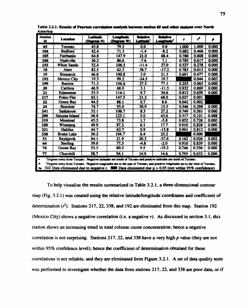
To help visualize the results summarizcd in Table 3.2.1. a three-dimensional contour
rnap (Fig. 3.2.1) was created using the relative latitude/longitude coordinates and coefficient of
determination (fi. Stations 217,22.338, and 192 are elirninated hm this rnap. Station 192
(Mexico City) shows a negative comlation (i.e. a negative r). As discussed in section 3.1. this
station shows an increasing trend in totai column ozone concentration; hence a negative
correlation is not suiprising. Stations 2 17.22. and 338 have a very high p value (they are not
within 95% confidence level); hence the coefficient of determination obtairred for these
correlations is not reliable, and they are elirninated from Figure 3.2.1. A set of &ta quality tests
was performed to investigate whether the data h m stations 217.22, and 338 are poor daîa, or if

isiocatcdinToFoato. T & ~ ~ a , w e â b ~ i n v e m e d & t m ~ e t o ~ ~ p ~ ~ r o f P ~ . The results art oaly signüiaat riithia Lbc box.
there W y is an anomaly that resulted in such poor correlations between those stations and
station 65. Each station was correiated with at least one other station close by. Station 217 was
correlateci with station 199; station 22 was correlated with station 64; and station 338 was
correlated with stations 21,241. and 320. Each correlation resulted in very srnail? and very
high p values. suggesting that stations 2 1.24 1, and 320 have poor &ta.
It is apparent h m Figure 3.2.1 that as distance i n c m away from Toronto, both in
latitude and longitude, the &ta h m station 65 becomes less representative of that area, with
highest comlations (70% and above) occurring within a radius of approximately 15O around
Toronto. This shows that while total ozone &ta obtained h m station 65 is not ~presentative
of the whole North America, it is representative of the Great Lakes region. It is. however, no

surprise that the data from station 65 is not representative of the whole North American
continent. In Section 3-1, it was demonstrated that there exists strong spatial variations in the
trend of total ozone concentration over the North American continent. The spatial variations
observed were attributed to the presence of various chernical and dynamical mechanisms of both
natural and anthropogenic origin. In Section 3.3, it will be shown that various natural cycles
such as QBO and solar cycles are refiected in total ozone data, and these cycles, which are
responsible for decadal, annual and inter-annual variations in concentration of total ozone. also
demonstrate spatial variations,
This finding helps WOLJDC in assessing the spatial distribution of their current ground-
based ozone monitoring stations. These stations are very costly both in terms of equipment used
and their maintenance, and also in terms of manpower utilized. Although it is necessary to have
at least two or three stations located close to each other for the purposes of data quality analysis,
at least sorne of the stations 104, 106, 155, 19, 20,21,22,24 1, 290, 3 19, 320,321, 338, and 64,
which fa11 within the 15" radius of Toronto, may perhaps be allocated to other locations such as
the northem pans of the Canadian West Coast where there are only few stations. Doing so will
result in more uniform data collection and hence will help better understand the spatial and
temporal variaîions in total column ozone concentration over North America.

3.3) SPECTRAL ANALYSIS: WHAT ARE THE NON-AHTHROPOGENIC SOURCES OF OZONE VARIATION?
To better understand the potential long-term effects of human activity on the
stratospheric ozone, it is necessary to understand first the natural long-term variability.
Therefore, the final objective of this study is to examine the natural sources of annual,
interannual. and decadai variation of total column ozone concentration over the study area, and
to further investigate any spatial variations resulting from these non-anthropogenic sources.
Time series spectral analysis is used to illustrate larger than seasonal time scaie
periodicities in the ozone data by identifying different frequency components. The objective is
to find those frequencies with the greatest spectrai densities, which contribute rnost to the
overall periodic behavior of the series (Statistica, 1995).
Since the seasonal periodicity of total column ozone concentration is very strong,
applying spectral analysis on monthly ozone data does not readily identify larger than seasonal
time scale trends in the ozone data (Fig. 3.3.1). Figure 3.3.1 is the spectral density for Toronto
using data from 1960 to 1999. As can be seen in Figure 3.3.1, there is a very strong peak at
f=0.083 which is equivalent to 12 months or 1 year. This peak clearly represents the seasonal
cycle component of the ozone data. Hence, in order to identify other long-term cycles in the
ozone data, the seasonal cycles should be minimized.

Various methods c m be used to either diminish or completely remove the seasonal
cycles. The seasonal decomposition methad often used in most studies is one where the original
series is seasonally adjusted by means of subtracting h m it (in case of additive series) or
dividing it by (for multiplicative series) the seasonal component. The seasonal component is
computed as the average (for additive series) or media1 average (for multiplicative series) for
each point in the season, i.e. the average of total column ozone concentration for aU months of
January within the given time series. This method was originaily suggested by Hill ( 1982) and
is widely used in most ozone studies. One problem however is that in most studies (Bojkov et
al., 1 990; Tung and Yang, 1994), the ozone data is treated as an additive series instead of a
multiplicative series. Many time series data contain seasonal periodicities, in order to
distinguis h between an additive and a multiplicative series; simple annual sales of toys can be
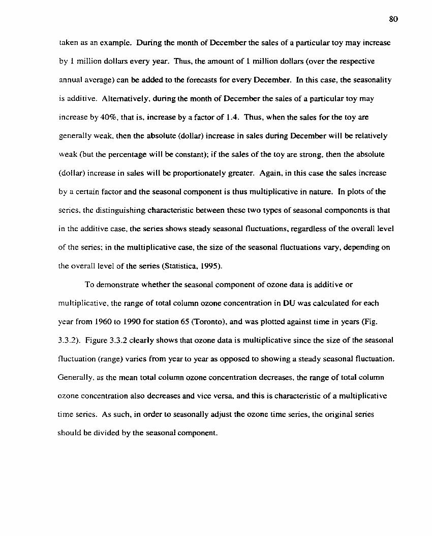
taken as an exarnple. Dunng the month of December the sales of a particular toy may increase
by 1 million dollars every year. Thus, the amount of 1 million dollars (over the respective
annual average) can be added to the forecasts for every December. In this case, the seasonality
is additive. Altematively, during the month of December the sales of a particular toy may
increase by 40%, that is, increase by a factor of 1.4. Thus, when the sales for the toy are
generally weak, then the absolute (dollar) increase in sales during December will be relatively
weak (but the percentage will be constant); if the sales of the toy are strong, then the absolute
(dollar) increase in sales will be proportionately greater. Again, in this case the sales increase
by a certain factor and the seasonal component is thus multiplicative in nature. In plots of the
series, the distinguishing characteristic between these two types of seasonal components is that
in the additive case, the series shows steady seasonal fluctuations, regardless of the overall level
of the series; in the multiplicative case, the size of the seasonal fluctuations Vary, depending on
the ovedl level of the series (Statistica, 1995).
To demonstrate whether the seasonal component of ozone data is additive or
multiplicative, the range of total column ozone concentration in DU was calculated for each
year from 1960 to 1990 for station 65 (Toronto), and was plotted against time in years (Fig.
3-32) . Figure 3.3.2 clearly shows that ozone data is multiplicative since the size of the seasonal
fluctuation (range) varies from year to year as opposed to showing a steady seasonal fluctuation.
Generally, as the mean total coiumn ozone concentration decreases, the range of total column
ozone concentration also decreases and vice versa, and this is charactenstic of a multiplicative
ti me series. As such, in order to seasonally adjust the ozone time series, the onginal series
should be divided by the seasonal component.

concentration
To test how effective this rnethod is in terms of minimizuig the seasonal cycles h m the
total column ozone tirne series. the method was apptied to data h m station 65 (Toronto). and a
spectral density analysis was then pefionned on the seasonally adjusted series (Fig. 3.3.3). As it
can be seen in Figure 3.3 -3. the seasonal cycle (€9.083) is significantly diminished as compared
to Figure 3.3.1. and other long-term cycles can now be detected. Before discussing the sources
of these other cycles. another seasonal decomposition method that was used in the previous
sections (Le. the 13-month mnning rnean) is discussed and compared to this rnethod.

Toronto, Cuuâa. Note: tbc scmmd cgck (f30.063) b still p-
The 13-month d g mean is anotkr mdiod thaî can be used to remove the seasonal
variations h m a time series. Using this method the ozone value for every month is calculated
as a mean of the data six months befote and afier. The running rnean method that is used in
Section 3.1, is also a helpfd graphical aid for visualizing any long-tenn patterns or apparent
trends in a time series (Hill, 1982). To test the effectiveness of this rnethod and to compare its
results with that in Figure 3.3.3, a spectrai analysis was p e r f o d on the 13-month ninning
mean data for station 65 and the results are shown in Figure 3.3.4.
As Figure 3.3.4 shows, the seasonal cycle (f=0.083) is fùrther diminished (although not
completely removed) as compared to Figures 3.3.1 and 3.3.3, and now other long-tenn trend
cycles can be detected more clearly. Hence this method proved to be more effective for
applkd) for &tim 65, TO&O, CM& Note: the aaml cyck (W.=) is b p m - b u t & ma& weaker.
diminishing seasonal cycles. However, it can be argued that this method can present a bias
since the first and the last month, which are in fact the same months in the tirne senes, are being
accounted for Nnce and this may somewhat alter the results of the s p c t r a i andysis. To remove
this potential bias, the 13-month mnning mean data for station 65 was recdculated. but this time
the first and the last months are given half weight. A spectrai analysis was perfonned on the
recdculated 13-month mnning mean data and the ~ s u l t s is shown in Figure 3.3.5.

It is evident in Figure 3.5.5 that the xecalculated Ifmonth running mean nwhod
completely removed the seasonal cycle and therefore it will be the method usbd for the
remainder of this section m m here on, whenever 13-manth nutning mean method is usei& it is
asswned thar the jïrst and the k t months are givcn half weight).
3.3.2) Lona-Term Cvcles Present in Tow C o l y ~ n Ozone nam
Having removed the seasonai cycle from Figure 3.3.5, the presence of other long-term
cycles cm now be detected. This graph shows the possible cycles that c m result in variations
of total ozone concentration at different time scales. More specifically eight distinct peaks crin
be identified in Figure 3.3.5. Figure 3.3.6 is essentially the same Figure as 3.3.5 only the x-
axis has been expanded and the ten peaks are marked and their corresponding periods have
been identified.
Peak 1 in Figure 3.3.6 (blue arrow) has a period of 39 years and it represents the length
of data used in the spectral analyses. It represents one full wave; from the beginning to end of
data, and its presence is merely an artifact. To investigate this further, we cut the length of data
in half and performed another set of spectral analyses. This time peak-one disappeared and
another peak with a period of 20 years emerged, confirming the source of pedc one as an
xtifact.
Peaks 2 (green arrow) has a period of approximately 9 years. This matches the solar
sunspot cycle period (Fig. 3.3.7) described in Section 1.5.1. To further examine this, a spectral
analysis was performed on the monthly solar sunspot data from 1960 to 1999 (Fig. 3.3.8). as
well as a cross-spectral analysis on the monthly solar sunspot data and total monthly column
ozone data for station 65 from 1960 to 1999 (Fig. 3.3.9). As Figure 3.3.8 shows, there is a
strong peak with a period of 10 years present in the spectrum of solar sunspot data.
Furthemore, in the cospectrum of sunspot and total ozone data, there is also a strong peak with
a period of approximately 9.6 years (i.e., f=0.0087). This peak is significant since the phase
spectrum at f=0.0087 is close to 2n radians (Fig. 3.3.10) and the amplitude of the squared
coherency peak at f=0.0087 (Fig. 3.3.11) is also high, confirming that the source of peak 2 in
Figure 3.3.6 is solar sunspot cycle activity, consistent with other results (Haigh, 1994).

13month running mtui applkd uid dttrradcd) for station 65, Toronto. The two major v o l a d c enaptions are marked.

65, Toronto) fnnn 1960 to 1999.

(station 65, Toronto) k m 1960 to l999.
(station 65, Toronto) trom 1960 to 1999

It is important to note that the solar activity minimum, for the last two solar cycles, has
coincidently begun at roughiy the same time as a major volcanic eruption (Fig. 3.3.7). This is
an example of two natural mechanisms, in phase with each other, resulting in higher than
normal variations of total column ozone concentration.
There is no clear explanation as to the source of peak 3 in Figure 3.3.6. One plausible
source is the El Niiio-Southern Oscillation phenomena described in Section 1.5.4. El NiRo is an
interannual oscillation that cornes at irregular intervals (2 to 7 years) and stays for an
unspecified penod of time, and each time with varying magnitude, therefore it is very difficult
to make a correlation between the period of peak 3 and that of El Nifio cycles.
The period of peaks 4 through 7 range between 1.7 to approximately 2.5 years. Peaks 4
and 5 are statistically significant and their p e n d matches the quasi-biennial oscillation (QBO).
The average penod of peaks 6 and 7 is 1.8 years (- 20 rnonths), but these peaks are not
statistically significant. According to Tung and Yang (1994) however, the 1.8-year peak,
thought not statistically significant in these results, is also a QBO signal coherent in al1
extratropical latitudes where there is a prominent seasonal cycle. This will be discussed in more
detail in the next section. To further substantiate that the period of QBO from 1960 to 1999
matches the perïod of peaks 4 and 5 , a spectral analysis was peiformed on QBO data from 1960
to 1999 (Fig. 3 -3.12). Furthemore, a cross-spectral anal ysis was also performed on mean
monthly total ozone data from station 65 and the QBO data froin 1960 to 1999 (Fig. 3.3.13).
Both Figures 3.3.12 and 3.3.13 show the same frequency peaks at 2.1 and 2.4 years, confirming
that the source of these peaks is likely the QBO cycle consistent with results of other studies
(Tung and Yang, 1994). Note, the cospectral peaks at 2.1 and 2.4 years are significant since
their phase spectrum is 27c radians (Fig. 3-3-14} and the amplitude of their squared coherency
peak (Fig. 3.3.15) is aIso high.


applied) and Singapore uni.l wind (QBO) at 30.mb, fmm 1964) to lm.
It can be concluded then, the natural variations in total ozone, aside from seasonal
cycles, can dso be related to quasi-biennial oscillations. to Sun spot activities, to volcanic
eruptions, and possibly to El Niiio-Southem oscillation. These cycles coexist and at any given
time, depending on their relative phase. they can amplify or miiigate ozone variability. For
example, the drastic decline in total ozone concentration that occurred between 1991 to the
middle of 1993 can be attributed to a solar activity minimum (Fig. 3.3.7) (which began in 1990).
the dominance of westerlies in tropical winds in the stratosphere between 1990 to 1993 (Fig.
1-52}, and to huge amounts of stratosphenc aerosol loading as the result of Mt. Pinatubo
volcanic emption that occurred in 1991. Knowledge of these cycles provides the basis for
realistic ozone forecasts.

3.3.3) Spâÿal Var(8Upns R e m o m Non amrowagnic -ce% . . L
To investigate any spatial variations resulting from the solar sunspot and the QBO cycles
over the study area, the same spectral analyses perforrned for station 65, using a Tukey window
with a window width of 3 months, is perforrned for some of the stations dong transects A, B,
and C (Fig. 3.1.16). The results are shown in Figure 3.3.16.
Though the information compiled in Figure 3.3.16 is variable, some general
observations can be made. One obvious feature is that the peak spectral density for stations
dong transect B (high-latitudes) are much larger than at other stations in rnid and low latitudes.
The second observation is that generally, similar to station 65, the spectral density peak for the
solar sunspot activity is greater than the spectral density peak for the QBO, suggesting that over
the study area, solar sunspot activity is a more dominant mechanism responsible for long-term
variations of total column ozone concentration. Finally, with respect to the QBO signal, most
stations in the mid and high latitudes, along with the 2.5-year QBO signal, also show a second,
and a relatively weaker signal with a period of 1.7 years. It should noted however, with the
exception of station 19, the second QBO peak is statistically fiot significant.
Ozone is mostly produced in the equatorial regions and then it is transported to higher
latitudes. For this reason, the total column ozone concentration in high latitudes (Le. stations
along transect B) is mostly dependent on the amount of ozone produced and transported from
the equatorial regions. Any Icng-term mechanisms (i.e. solar cycle and QBO) resulting in the
variations of total column ozone concentration may not be readily evident in the spectral
analyses of lower latitude stations as these long-term signals are damped due to large arnounts
of excess ozone production in low latitudes. In high latitudes however, since in situ ozone
production is minimum and the total ozone concentration is highly dependent on the
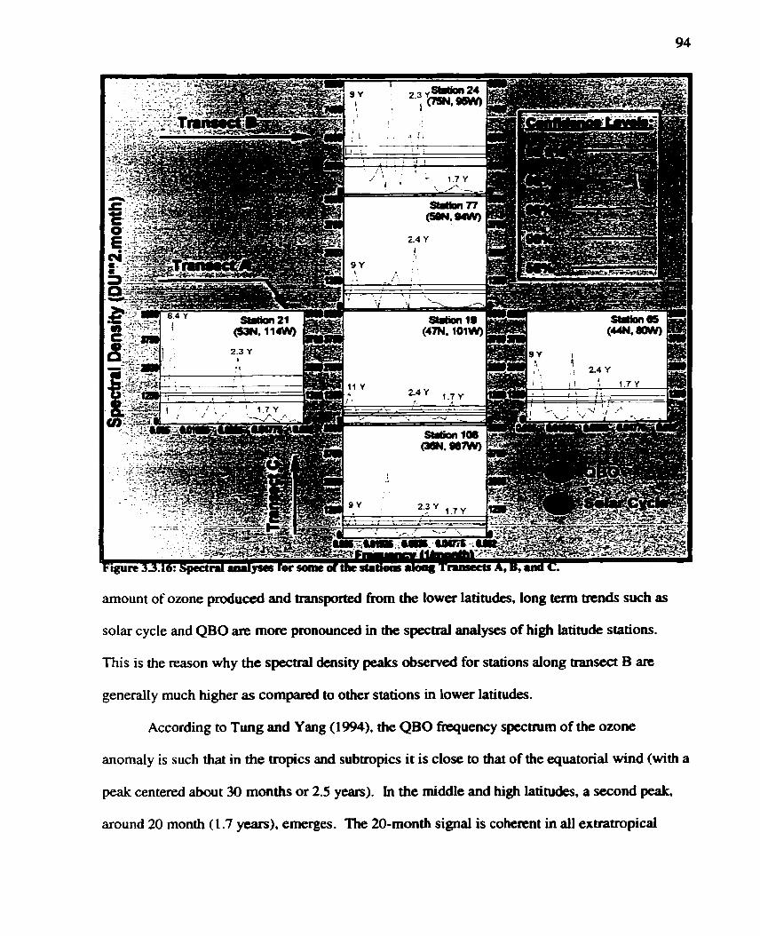
amount of ozone produced and transported from the lower latitudes. long iam trends such as
solar cycle and QBO are more pronounced in the spectral analyses of hi* latitude stations.
This is the reason why the spectral density peaks observed for stations dong transect B are
generally much higher as compaRd to other stations in lower latitudes.
According to Tung and Yang (1994), the QBO frequency spectrum of the ozone
anomaiy is such that in the tmpïcs and subtropics it is close to that of the equatorial wind (with a
peak centered about 30 months or 2.5 years). In the middle and high latitudes, a second peak,
around 20 month ( 1.7 years), emerges . The 20-month signal is cohennt in aîi extratropical

latitudes, including the polar latitudes. These results are in agreement with Our findings (Fig.
3.3.16) although in our analyses, it is shown that for most stations, the second peak is
statistically not significant. Tung and Yang (1994) also detected an 8.6-month spectral peak that
is much fainter than those at 20 and 30 months. This 8.6-month spectral peak is not present in
our analyses due to the 13-month running mean applied to the monthIy total column ozone data
in order to remove the seasonal cycles.
To explain the presence of this 3-peak QBO signal, Tung and Yang (1994) argued that
such extratropical QBO anomalies should exist in the transporting circulation itself (and
therefore should exist in the wave Eliassen-Palm flux divergence) through a dynarnical
mechanism. This theory States that the dynamical QBO should act to modulate the annual cycle
(or vice versa) in the extratropics in the following way. Consider a 30-month harmonic, Q(t).
that acts to modulate an annually periodic function, F(t), consisting of an annual mean and a
1 1 1 1 1 1 sinusoid with an annual period. Then, since , + ~3 G =and z- 30 G 30, we have:
The result is a three-peak spectrum (30, 20, and 8.6 months) for the product (Baldwin and Tung,
1994).

4.0) CONCLUSIONS AND RECOMMENDATIONS
In this thesis the history and conceptual understanding of the processes responsible for
production and destruction of ozone, its global distribution, as well as mechanisms responsible
for annual, interannual and decadal variations of total column ozone concentration have k e n
reviewed.
The pnmary aim of this study was to examine the status of total column ozone
concentration over North Amenca. It was detennined that the total column ozone concentration
has been decreasing over North Amenca and this negative trend exhibits strong latitudinal
variations. The magnitude of this negative trend increases with latitude in the midlatitudes with
a relative drop in the magnitude in the high-latitudes. The maximum trend in total column
ozone reduction is approximately 8.3% per decade in the midlatitudes while in high-latitudes it
diminishes to 3.8% per decade. These findings are in agreement with broader global studies
(Bojkov and Fioletov, 1995) that have calculated a cumulative year-round decline in middle and
high latitudes total column ozone concentration of 6.3I1.5% per decade.
While many studies have acknowledged the existence of Northern Hemispheric
midlatitude ozone reduction, they mostly focus on the cumulative trend of Northern
Hemisphenc column ozone reduction and do not draw attention to the fact that relatively higher
trends have occurred in the midlatitudes as compared to the high-latitudes. In this respect, Our
finding is unique. There are many different chemical and dynamical mechanisms that have k e n
proposed in various studies that each can contribute to at least part of the observed midlatitude
ozone decline. While these mechanisms can al1 coexist, their effects could dominate during

different seasons. Hence, a combination of several such effects jointly considered can give a
possible ex planation for the observed rnidlati tude trends in total column ozone concentration.
Aside from latitudinal variations, temporal variations in total column ozone
concentration have also been detected. It was found that while high latitude stations
demonstrate a slightly positive trend in total column ozone concentration for the p e n d of f 975
to 1985, midlatitude stations show the largest rate of total ozone reduction during this period.
Conversely, while the rate of total ozone reduction increases considerably during the period of
1985 to 1995 in high-latitudes, midlatitude stations demonstrate a slight decrease in the rate of
total ozone reduction (a sign of leveling off) during this period.
The large rates of total column ozone reduction observed between 1975 to 1985, in
midlatitudes, are evidence for the important role that heterogeneous chemistry plays in
midlatitude ozone depletion and further emphasizes the importance of anthropogenic sources
with respect to ozone depletion. Moreover, the "leveling off' that has occurred in midlatitude
ozone trends between 1985 to 1995 is perhaps attributed to the Montreal Protocol signed in
1989 which required a 50% reduction in CFC emissions by mid-1998. The Mt. Pinatubo
eruption in 1991 seems to be the main cause of the unusuaily negative trend in total column
ozone concentration observed over the whole of North Amenca between 1985 to 1995. If this
eruption had not occurred, the Montreal Protocol might have led to perhaps even greater
decreases in the rate of total column ozone reduction in the midlatitudes during this period.
Natural sources of total column ozone variations that are responsibie for inter-annual and
decada1 variations of total ozone over the study area have also k e n examined. The soiar
sunspot activity and QBO are deemed to be the two main sources of long-term ozone variations
over North America, with solar sunspot activity being the more dominant source. The El Nifio-
Southern Oscillation is perhaps yet another source of inter-annual variations of total column
ozone over North America, but a statistical link was not established in this study. It is important
to note that these natural cycles coexist and at any aven time. depending on their relative phase,
can amplify or rnitigate ozone levels. Hence, knowledge of these cycles provides the basis for
realistic ozone forecasting and will help better understand the potential long-term effects of
human activity on the stratosphenc ozone and vice versa.
It was also shown that seasonal oscillations that cause annual variations of total column
ozone concentration are very strong. Therefore, before performing any meaningful statistical
analysis on ozone data, the seasonal cycles should be removed. Various techniques were
examined in this thesis, and it wss demonstrated that the 13-month running mean method is
most effective in terms of removing the seasonal cycles from the ozone data and is a helpful
graphical aid for visualizing any long-term patterns or apparent trends in a time series.
Lastly, using the total column ozone data from Toronto, it was determined that data
obtained from the ground-based Dobson-Brewer spectrometers are representative of an area
approximately 15" in radius. This suggests that ozone data from Toronto are representative of
the Great Lakes region. But it also suggests that some of the WOUDC stations that are highly
clustered within Southern Ontario and the Prairies should be allocated to other locations where
they are more needed i.e., northern parts of the Canadian West Coast where there is a scarcity of
stations. Doing so will result in overall higher spatial resolution and hence will help us to better
understand the spatial and temporal variations in total column ozone concentration over North
America.
This study mainly focused on the annual trends of total column ozone concentration.
The total column ozone concentration exhibits strong seasonal variations. In the midlatitudes
for instance, the total colurnn ozone maximum is reached in the spring, while the minimum is
usually obsewed in the fall. The chemical and dynarnical mechanisms potentially responsible

for midlatitude ozone decline can each be dominant during different seasons. For example,
transport of ozone-depleted air from the polar vortex could lead to large spring ozone depletion.
Changes in atmospheric dynamics can affect ozone, but its effect is mostly maximized during
winter. Hence, to gain better insight into the spatial and temporal variations of totd column
ozone concentration over North America, it is recommended that future studies divide the data
sets into the four seasons and perforrn similar analyses on each season separately. In this
manner, seasons responsible for maximum or minimum rates of ozone destruction cm be
identified, and hence, the relative importance of some of the midlatitude-ozone-destroying
mechanisms proposed in Section 1.6, can be assessed. A possible temporal variation in the rate
of total ozone destruction for different seasons, if observed, can gain funhet insight into the
relative importance, and the evolution, of some of these midlatitude-ozone-destroying
mechanisms.
The final recommendation is to perfonn sirnilar analyses as was done in Section 3, on
Ozonesonde data. The Ozonesonde data, although not as widely avaitable as the Dobson-
Brewer spectrometer data, c m also be retrieved from the WOUDC database. The Ozonesonde
data is ri measurement of ozone concentration at different dtitudes. Hence, a time series
analyses of this dataset can provide information on possible spatial and temporal variations of
ozone at different altitudes, thereby providing a 3-dimensional view of long-term trends of
stratospheric ozone over North America.

Atlas, E., W. Pollock, J. Greenberg, L. Heidt, and A.M. Thompson, 1993. Alkyl nitrates. non- metitane ltydrocarbons, and halocarbon gases over the equatoriul PaczjTc Ocean drtring gSAGA3. Journal of Geophysical Research-Atmospheres, 98, 16933- 16947.
Baldwin, M.P., and K.K. Tung, 1994. Exrra-tropical QBO Signals in Angular Momentum and Wave Forcing. Geoph ysical Research Letters, 2 1: (24), 27 17-2720.
Bekki, S ., 1997. On the possible role of aircrafr-generated soot in the middle laritude ozone depletion. Joumal of Geophysical Research-Atrnospheres, 102: @9), 1075 1 - 10758.
Blake. D.F., and K. Kato, 1995. Latitudinal distribution of black carbon soot irt the ripper troposphere and lower strarosphere. Joumal of Geophysical Research-Atmosphere, 100, 7 195-7202.
Bojkov, R., L. Bishop, W.J. Hill, G.C. Reinsel, and G.C. Tiao, 1990. A statistical trend analysis of revised Dobson total ozone data over the northem hernisphere. Joumal of Geophysical Research-Atmospheres, 95,9785-9807.
Boj kov, R., and V.E. Fioletov, 1995. Esrimathg the global ozone characteristics dziring the fast 30 years. Joumal of Geophysicd Research-Atmosphere, 100: @8), 16537-1655 1.
Bojkov, R., V.E. Fioletov, and A.M. Shalamjansky, 1994. Total ozone changes over Erirasia sirzce 1973 based orr reevalriatedfilter ozonorneter data. Journal of Geophysical Research-Atmospheres, 99: (D 1 l), 22985-22999.
Borrmann, S., S. Solomon, J.E. Dye, and B. Luo, 1996. Tlie potenrial of cirrus clorids for Izeterogeneozis chlorine activation. Geophysical Research Letters, 23, 2133-2 136.
Bormann, S., S. Solomon, L. Avallone, and D. Baumgardner, 1997. Tlie relationship benveen CIO and aerosol surface area in cirnis clouds and volcanic aerosol near the midlatitude tropopause. Geoph ysical Research Letters, 24: (1 6) 20 1 1-20 14.
Bossert, J. E., 1997. Art Investigation of Flow Regimes Affecting the Mexico City Region. Journal of Applied Meteorology, 36: ( 3 , 119-140.
Chandra, S., C. Varotsos, and E. FIynn, 1996. nie mid-latitude total ozone trends in the ~zortizenz hernisphere. Geophysical Research Letters, 23: (3, 555-558.
Chartrand, D.J., J. de Grandpre, and J-C. McConnell, 1999. An introduction to Stratosplieric Chemisrry . Atmosphere-Ocean, 37: (4), 309-367.
Chatfield, R.B., and P.J. Crutzen, 1984. Suifïtrdioxide in remote oceanic a ic Cloud transport of reacrive precursors. Joumal of Geophysical Research-Atmospheres, 89,7 1 1 1-7 132.
Clark, W.A.V., and P.L. Hosking, 1986. Statistical Methods for Geom~hers . John Wiley & Sons, Inc.
Danielsen, E.F., 1993. In situ evidence ofrapid, vertical. irreversible transport of lower troposphenc air into the lower tropical stratosphere by convective clorrd turrets and by larger scale uprvelling in tropical cyclones. Journal of Geoph ysicd Research- Atmosphere, 98, 8665-868 1.
De Winter-Sorkina, R., 1995. k ~ l e t i o n and Natural Variabilitv of the ozone Laver from TOMS Observations. Rep. 722201005,91 pp., Nat. Inst. Of Public Health and Environ. Prot., Air Res. Lab., Bilthoven, Netherlands.
Dobson, G.M.B., and D.N. Harrison, 1926. Measurement of the amortnt of ozone in the Eadt's ripper atnzosphere and irs relation to other geophysical conditions. R. Soc. (London) Proc. ser. A, 110,660-693.
Douglass, A.R., R.B. Rood, J.A. Kaye, R.S. Stolarki, D.J. Allen, and E.M. Larson, 1991. ïXe i~zJTrtence of polar heterogeneous processes on reactive clzlorine ut midlatitudes: rltree- dirnertsional mode1 implications. Geophysical Rcsearch Letters, 18: (1)- 25-28.
Environment Canada, 1998. Ozone Science: A Canadian Perspective on the Changing Ozone Layer. http:/lexpstudies.tor.ec.gc.ca/e/ozone/download~ozone~science. htm.
Fabry, C., and M. Buisson, 1921. Etude de l'extreniite ultraviolette dit spectre solaire. J. Phys. Rad., 3, 197-226.
Fast, J. D., and S .Y. Zhong, 1998. Mereordogical factors associated witli inlzomogeneoirs ozone concentrations rvitliin tlze Mexico City basin. Journal of Geophysical Research- Atmospheres, 103: (Dl 5), 18927- 18946.
Firor, J., 1990. The Channine Atmos~here. A Global Challenne. Yale University Press, New Have. 143p.
Fortuin, J.P.F., and H. Kelder, 1996. Possible liriks benveen ozone and tentperatirreprofiles. Geophysical Research Letters, 23, 15 17- 1520.
Fusco, A.C., M.L. Salby, 1999. Interannual variations of total ozone and rlieir relationskip to variations of planetary wave activity. Journal of Climate, 12: (6), 1619-1629.
Gidel, L.T., 1983. Cuniulus cloud transport of transient tracers. Joumal of Geophysical Research-Atmospheres, 88,6587-6595.
Gotz, F.W.P., A.R. Meetham, and G.M.B. Dobson, 1934. The vertical distriburion of ozone in the atrrzosphere. R. Soc. &ondon) Proc., ser. A, 145,416-446.
Granier, C., and G. Brasseur, 1992. Impact of Heterogeneous Chemistry on Mode1 Predictions of Ozone Changes. Journal of Geophysical Research-Atmospheres, 97: @IO), 18015- 18033.

Greenwood, B., 2000. Personal Communication, University of Toronto, Canada.
Haigh, J-D, 1994. Tlie role of stratosplreric ozone in rnodulating the solar radiative forcing of cl irnate. Nature, 370, 544-446.
Hami l ton, K., 1998. Dynarnics of the Tropical Middle Atmosphere: A Tutorial Review. Atmosphere-Ocean, 36: (4), 3 19-354.
Hartley, W.N., 1881. On the absorption spectnrrn of ozone. Chernical Society Journal (London), 39, 57-60.
Hill, J.W., 1982. Ozone Trend Analysis. In: Bower, A.F., and B.R. Ward. Stratospheric Ozone and Man. Volume 1. CRC Press, Inc. Boca Raton, Florida. 70-86.
Hood, L. L, 1997. TIte solar cycle variation of total ozone: Dynarnical forcing in the lower stra?osphere. Journal of Geophysical Research-Atmosphere, 102: @ l), 13%- 1370.
Hood, L.L., J.L. Jirikowic, and J.P. McCormack, 1993. Quasi-Decadal Variability of the Stratosphere: hzjluerice of Long-Tenn Solar Ultraviolet Variatiorzs. Journal o f the Atmosphere and Sciences, 50: (24), 3941-3958.
Hood, L.L., J.P. McConnack and K. Labitzke, 1997. An investigation of dynarnical cori?ribritions to midatitude ozone trends iri winter. Journal of Geophysical Research- Atrnospheres, 102: (Dl 1), 13079-13093.
Hood, L.L., and D.A. Zaff, 1995. Lower stratosplieric staiionary waves and the longitude dependence of ozone trends in winter. Journal of Geoph ysical Research-Atmospheres, 100: @ 12), 2579 l-258ûû.
Hosseinian, R., and W. Gough, 2000. Tora1 colttmn ozone variability over Toronto, Ontario, Ca~zada. Great M e s Geographer, 7, (in press).
Houghton, T. J., 1986. The Phvsics of Atmos~heres. Cambridge University Press. Cambridge, U.K. 271p.
James, N, I., 1994. Introduction to Circulating Atmos~heres. Cambridge University Press. Cambridge, U.K. 422p.
Jones, R.L., and A.R. MacKenzie, 1995. Observatiorial strrdies of the role of polar regioris in rnidlatitude ozone loss. Geoph ysical researc h letters, 22: (24), 3485-3488.
Kritz, M.A., S.W. Rosner, K.K. Kelly, M. Loewenstein, and K.R. Chan, 1993. Radon nreasri retneizts in the lower tropical stratosphere: Evidence for rapid vertical transport and deliydration of rropospheric air. Journal of Geophysical Research-Atmosphere. 97, 8725-8736.

Kinnersley, J.S., and K.K. Tung, 1998. Modeling the global interannual variability of ozone due to tlze equatorial QBO and to enratropical planetary wave variability. Journal of the Atmospheric Sciences, 55: (8), 1417-1428.
Kowalo k, E .M., 1993. Research Lessons fiom Acid Rain, Ozone Depletion. and Global Wanning. Environment 35: (6), 13-38.
Lary, D.J., Lee A.M, and Tourni R., 1997. Carbon aerosols and amosphenc photochemistry. Journal of Geophysical Research-Atmospheres, 102: @3), 367 1-3682.
London, J., 1985. Distribution of Atmospheric Ozone. In: R.C. Whitten, and S.S. Prasad. Ozone in the Free Atmos~here. Van Nostrand Reinhold Company. New York. 1 1-80.
London, J., and K.J. Angell, 1982. nze observedDistribution of Ozone and its Variations. In: A. F. Bower, and B.R. Ward. Stratos~heric Ozone and Man. Volume 1. CRC Press, Inc. Boca Raton, Fionda. 8-36.
iMap.com, 2000. Satellite image of the North Arnerican Continent. www.map.com.
McCormack, J.P., and L.L. Hood, 1997. Modeling the spatial distribitrion of total ozone in rtonhern hemisphere wintec 1979-1991. Journal of Geophysicai Research- Atrnospheres, 102: @12), 1371 1-13717.
NGDC, 2000. National Geophysical Data Center. http://www.ngdc.noaa.gove/.
Niu, X., J.E. Fredeïick, M.L. Stein, and G.C. Tiao, 1992. Trends in colztrnn ozone based on TOMS data: Dependence otr month, latitude, and lorzgitude. Journal of Geophysical Research-Atmospheres, 97, 1466 1 - 14669.
Peters, D., and G. Entzian, 1996. January ozone anomaly over tlze North Arlantic-European regiot 1: 1 or zgitude-dependent decudal change in total ozone during 1979- 1992. MeteoroI. 2. N. F., 5,4145.
Peter, T., 1994. The strotospheric Ozone Layer-An Overview. Environmental Pollution, 83: (1-2), 69-79.
Pickering, K., A.M. Thompson, J.R. Scala, W.K. Tao, and J. Simpson, 1992. Ozone production pore~ttid folloiving convective redistribution of biomass buming emissions. Journal of Atrnospheric Chemistry, 14, 297-3 13.
Proffitt, M.H., J.J. Margitan. K.K. Kelly, M. Loewenstein, J.R. Podolske, and K R . Chan, 1990. Ozone loss in the Arctic polar vortex in ferred from higlr altitude aircrafi measrirenzertts. Nature, 347, 3 1-36.
Proffitt, M.H., K. Aikin, J.J. Margitan, M. Loewenstein, J.R. Podolske, S.E. Strahn, and A. Weaver, 1993. Ozone loss inside the nodtem polar vortex during the 1991 - 1992 ivirtter. Science, 26 1, 1 150- 1 154.
Randel, W.J., and J.B. Cobb, 1994. Coherent variations ofmonthly mean total ozone and lower stratospher+c temperature. Journal of Geophysical Research-Atmospheres, 99,5433- 5447.
Randel, W .J., F. Wu, 1995. TOMS total ozone trends in potential vorticity coordinates. Geophysical Research Letters, 22: (6), 683-686.
Rasmussen, R.A., M.A.K. Khalil, R. Gunawardena, and S.D. Hoyt, 1982. Atmospheric methyl iodide (CH31). Joumal of Geophysical Research, 87,3086-3090.
Regener. E., and V.H. Regener, 1934. Aufiahmen des ultraviolerten Sonnen-spetnrms in der Srratosphare und die verfikale ozonverteilung. Phys. Z., 35,788-793.
Reifenhauser, W., and KG. Heumann, 1992. Determinations of rnethyl iodide in the Antarctic atmospllere and the sourh polar sea. Atrnospheric Environment, 26 (A), 2905-29 12.
Shen, L. T., J.P. Wooldridge, and J. M. Molina, 1995. Stratosphericpollurion and ozone depletion. In: Singh, B. H. Comwsition. Chemistw, and Climate of the Atmosphere. Van Nostrand Reinhold. New York. 394-442.
S hiotani, M., 1992. Amual, quasi-biennial and El Nino-Sorrthern Oscillation (ENSO) time- scale variations in equatorial totul ozone. Journal of Geophysical Research- Atmosphere, 97,7625-7633.
humwaÿ, R.H., 1988. Aa~Iied Statistical Time Series Analvsis. Prentice Hall, Englewood Cliffs, New Jersey. 379p.
ingh, H.B, L.J. Salas, and R E . Stiles, 1983. Metkylhalides in and over the eastem Pacific (40 W-32 3). Joumal of Geophysical Research-Atmosphere, 88,3684-3690.
Soiomon, S., R.R. Garcia, and A.R. Ravishankara, 1994. On the role of lodine in Ozone depletion. Joumal of Geoph ysical Research-Atmospheres, 99: (D IO), 2049 1-2û499.
Solomon, S., R. W. Portmann, R.R. Garcia, L.W. Thornason, L.R. Poole, and M.P. hkConnick, 1996. The role of aerosol variarions in anthropogenic ozone depletion at nortltem midlatitrcdes. Joumal of Geophysical Research-Atmospheres, 10 1 : @3), 67 13-6727.
Soiomon S., S. Bormann, R.R. Garcia, R. Portmann, L. Thornason, Poole L.R., D. Winker, and M.P. McCormick, 1997. Heterogeneoits cldorine cltemistry in the tropopause region. Journal of Geophysical Research-Atmosphere, 102: (D l7), 2 141 1-21429.
Soukharev, B., 1997. The sunspot cycle, the QBO, and the total ozone over Northeastem Erirope: a connection throirgh the dynamics of stratospheric circulation. Annales Geophysicae-Atrnospheres Hydrospheres and Space Sciences, 15: (12)- 1595-1603.
S tatistica, 1995. Tirne SeriedForecasting. Statistica Manual, 95 Edi tion, Volume 3. StatSoft. Inc. U.S.A., 366p.

S tolarski, R.S., P. Bloomfield, R.D. McPeters, and J.R. Herrnan, 199 1. Total ozone trends dediiced from Nimbus 7 TOMS data. Geophysical Research Letters, 18: (6)-, 10 15- 10 18.
Stolarski, R.S., R. Bojkov, L. Bishop, C. Zerefos, J. Staehelin, and J. Zawodny, 1992. Measitred trends in stratospheric ozone. Science, 256: (5055), 342-349.
Strutt, R.J., 19 18. Ultraviolet transparency of the lower atnzospkere and its relative poverty in ozone. R. Soc. (London) Proc., ser. A, 94, 260-268.
Tie, X.X., and G. Brasseur, 1995. The response of Stratospheric ozone to Volcanic-Emptions- Sensitivizy to Atmospheric chlorine loading. Geophysical research letters, 22: (22), 3035-3038.
Tourpaii, K., X.X. Tie, C.S. Zerefos, and G. Brasseur, 1997. Decadal evoltition of total ozone decline: Observations and mode1 results. Journal of Geoph ysical Researc h- Atmosphere, 102: (D20), 23955-23962.
Tuck,A.F.,D.W.Fahey,M.Loewenstein, J.R.Podolske,K.K. Kelly,S.J.Hovde,D.M. Murphy, and J. W. El kins, 1994. Spread of denitrification from the 1987 Antrctic and 1988- 1989 Arctic stratosplteric voriices. Joumal of Geophysical Research-Atmosphere, 99,20573-20583.
Tuck, A.F., J.M. Russell III, and J.E. Harries, 1993. Stratosplzeric dryness: Antipliased desiccatioti over Micronesia and Antarctica. Geophysical Research Letters, 20, 1227- 1230.
Tuck, A.F, T. Davies, S.J. Hovde, M. Noguer-Alba, D.W. Fahey, S.R. Kawa, K.K. Kelly, M.H. Proffitt, J.J. Margitan, M. Loewenstein, J.R. Podolske, S.E. Strahan, and KR. Chan, 1 992. Polar stratospheric cloud processed air and poterttial vorricity in the Northem Hemispliere lower stratosphere ut rnidlatitudes drtring rvinter. Journal of Geophysical Research-Atmosphere, 97: (Dg), 1 1 18 1-1 1233.
Tung, ECK, and H Yang, 1994. Global QBO in Circulation and Ozone. I . Reexarnination of Observational Evidence. Joumal of the Atmospheric Sciences, 5 1: (19), 2699-2707.
Turco, R.P., 1985. Stratosplzeric Ozone Perturbations. In: R.C. Whitten, and S.S. Prasad. Ozone in the Free Atmos~here. Van Nostrand Reinhold Company. New York. 195- 242.
WapIe, A. M., 1999. The sttn-climate relationship in recent centtiries: a revietv. Progress in Physical Geography 23: (3), 309-328.
Whitten, R.C., and S.S. Prasad, 1985. Ozone in the Free Atmos~here. Van Nosuand Reinhold Company. New York. 288p.
Wi 1 Ii am, V., and R. Toumi, 1999. Tlie Radiative-Dynamical Eficts of High Cloud on Global Ozone Distributiorz. Joumal of Atmospheric Chemistry, 33, 1-22.
World Meteorological Organization (WMO), 199 1. Scientific assessrnent of ozone de~letion: 1991. Rep. 25, Worid Meteorolog. Organ., Ozone Secr., Geneva. Switzerland. -
World Meteorological Organization (WMO), 1995. 1994 Assessrnent of Ozone Depletion. Rep. 37, World Meteorolog. Orgm., Ozone Secr., Geneva, S wi tzerland.
WOUDC, 3000. Word Ozone and Ultraviolet Radiation Data Center. http://www.msc- smc.ec.gc.ca/woudc/index.htmi.
Zerefos, CS., A.F. Bais, I.C. Ziomas, and R.D. Bojkov, 1992. On the relative importarice of quasi-biennial oscillation and El Nino/sourtiem oscillation in fhe revised Dobson total ozaize records. Journal of Geophysical Research-Atmospheres. 97: (D9), 10135-10 144.

APPENDlX A) DETERMDNATDOW OF TOTAL COLUMN OZONE
The Dobson spectrophotometer is the designated standard instrument for total ozone
rneasurements in ihe global network, and it is used as a calibration base for a number of other
total ozone observing systems, incIuding those involving satellite techniques (London, 1985).
It is a double prism monochrometer that matches radiance measurements at two different
wavelengths about 20 nm apart, in the Huggins bands of the ozone ultraviolet spectrum (300-
340 nm). An optical wedge is used to reduce the observed radiance at the weaker absorbed
wavelength. A nul1 setting then ailows the relative radiance, and thus the total ozone amount in
the vertical column, to be determined through the following equation:
where subscripts 1, 2 refer to wavelengths of relatively strong and weak ozone absorption respectiveiy;
X is the total arnount of ozone in a vertical column in Dobson Units (1 Dobson Unit i.e. DU, is defined as 0.01 mm thickness at STP i.e. zero degrees Celsius and 1 atmosphere pressure);
L and Laare the measured radiances at the ground and the top of the atmosphere respectively;
a; p, and Gare the decadic ozone absorption (cm-'), molecula. scattering for air (atmo~~here'l). and aerosol scattering (relative) coefficient;
n i is the optical path length allowing for refraction through the molccular scattering for a spherical atmosphere;
p. po are the station pressure and mean sea level pressure respectively;
J is the solar zenith angle; and
,IX is the relative path length of the solar beam through the ozone layer for a spherical atmosphere (London, 1985).

Detemination of total ozone by the Dobson method (London, 1985) is based on a
number of assurnptions. They are:
the major part of the ozone layer is in the lower or middle stratosphere,
the relative radiance received at the top of the atmosphere for the different wavelength
pain does not change with tirne, e-g., during the course of different sunspot cycles,
UV absorption in the atmosphere at the observed wavelengths is by ozone alone, and
the wavelength dependence of atmosphenc aerosol scattering is, for the observed spectral region, linear in first-order differences,
Total ozone observations cm be made for solar zenith angles as large as about 80".
Although the observations are most reliable when viewing the sun directly (i.e., at noon), useful
routine measurements can also be made under other conditions (e.g., viewing the zenith sky
under clear or cloudy conditions, or direct observation on the moon). Different wavelength
pairs are then combined to fit the different observing condition as appropriate (London. 1985).
Since the Dobson spectrophotometer is the designated standard instrument for total ozone
measurements, it is important to consider the sources of uncertainty in the Dobson
measurements. According to London (1985), these errors involve':
1. the possible inaccuracy of the effective ozone absorption coefficients used with the Dobson spectrophotometer and the temperature dependence of these coefficients,
2. the possibility of interference in the radiance measurements due to the presence of trace gases with absorption spectra near wavelengths used in the Dobson instrument,
3. instrumental errors of various types, including the detenoration of the interna1 optics, the presence of scattered light within the instrument, and the possible drift of the optical wedge characteristics,
4. possible nonlinear variation of aerosol scattering coefficient in the Huggins band,
5. variable extraterrestrial solar radiance at wavelengths used in the Dobson instrument, ar?d
' For a detaii discussion of tbese errors, their relative importance. and correction methods used to minimize these errors. please refer CO London (1985).

6. the need for correction for polarized light associated with zenith or cloudy sky observations.
A program has k e n developed by the World Meteorological Organization (WMO) for
routine intercalibrations of a set of nine regional standard Dobson instruments with World
Primary Standard Dobson Spectrophotometer No. 83 operated in the U.S. by NOAA, Air
Resources Laboratory, Boulder, Colorado, designated by the WMO as the World Dobson
Spectrophotometer Central Laboratory. The regional standard spectrophotometers are used
periodically to calibrate other instruments in the Global Network (London, 1985 and references
therein).
A new spectrophotorneter was designed by Brewer in 1973, based partially on a mode1
constructed by Wardle in 1963, as an improvement on the Dobson instrument that would
minimize the difficuity of taking observations under different atmospheric conditions. The
Brewer instrument, intended as a replacement for or supplement to the Dobson
spectrophotometers used in the global ozone observing network, is a grating spectrophotometer
designed to measure the solar radiance at five wavelrngths in the spectral interval 306-320 nm
with a resolution of 0.6 nm (the Dobson spectral resolution is about 1 .O-1 -5 nm). Calculations
of total ozone with the Brewer instrument follow the Dobson method using paired wavelengths
as given in Eq. (A- L). The radiance at each wavelength, however, is measured by a pulse
counting system that eliminates the need for the troublesome optical wedge. The instrument has
intemal calibration capability and is still smali enough to be portable. Through use of a
polaizing pnsm, reasonably accurate observations on a clear or cloudy zenith sky can be made
without the need of an empirical chart. In addition, observations of the wavelengths adopted for

use with the Brewer instrument can be combined to provide information for determining the
column abundance of SOz. This information can be used as a correction factor in total ozone
observations taken in heavily polluted air. Results of extensive field programs have shown an
rms difference in computed total ozone amounts of less than 1% when Brewer and Dobson
measurements are compared (London, 1985 and references therein).
The M-83, employed chiefly in the USSR and Eastern Europe, was originally based on
the measured ratio of the solar irradiance received in three relative1 y broad spectral intervais in
the Huggins bands (-300-340 nm). The insuurnent was later modified to employ two filters for
total ozone measurements centered at 304 nm and 330 nm. Total ozone is then derived from the
measurements of the ratio of the received radiance at the two different wavelengths (see Eq. A-
l), at different instrument temperatures and solar zenith angles, with the aid of a calibration
nomogram that is provided for each station using ar! M-83. The major error arising from the use
of the M-83 involves the standardization and calibration of the broad band-pass optical filten
and the large field of view of the instrument (6"). Relatively large errors (up to 20%) in the
reported total ozone amount occur at low solar elevations, primarily because of the shift of the
effective central wavelength of maximum filter transmission as a function of the solar zenith
angle. Significant errors also occur when observations are made in the presence of large aerosol
concentrations. Routine direct Sun or zenith blue-sky observations made with the M-83 are
much more reliable than those taken through cloudy skies (London, 1985 and references
therein).
The two principal techniques used for satellite measurements of total ozone involve
observations of solar ultraviolet radiation which has been backscattered from the earth and
atmosphere, or observations of infrared emission at 9.6 p n from the ground and atmosphere
(London, 1985 and references therein).
The backscattered ultraviolet (BUV) method measures the portion of upwelling solar
radiation that has been intercepted by ozone dong the path of the solar beam and then scattered
back to the satellite by the earth and atmosphere. The principles of the method are very similar
to those involved in the Dobson technique. In the case of BUV observations, some difficulties
have been encountered largely because of instrument degradation and uncertainty of the correct
effective ozone absorption coefficients for the wavelengths used in the BUV instrument, and
because the presence of cloud layers requires some approximations for contributions of
troposphenc ozone to the total amount. As a result. irnprovements have been made on the
original design of the BUV instrument and procedures for determining total ozone arnounts with
the new instruments. These have been incorporated in the SoIar Backscatter Ultraviolet (SBUV)
and the Total Ozone Mapping Spectrometer (TOMS) instruments both flown on thz Nimbus-7
satellite (London, 1985 and references therein).
The total arnount of ozone in a vertical colurnn above the earth's surface or cloud top can
also be detemiined from satellite observations of the upward-directed infrared radiance in the
9.6 pm ozone band provided that the vertical temperature distribution is known. The method for
data reduction requires the solution of an integral equation that is not very well known, as a
result a set of approximations is used whereby total ozone, as observed from ground-based
Dobson measurements, is correlated with clear sky radiances observed by the satellite
instrument. This method has been used with the Nimbus-3 and Nimbus-4 IRIS system, the

Defense Meteorologicd Satellite Program-Multichannel Filter Radiometer (MF'), the TIROS
Operational Vertical Sounder (TOVS), and METEOR 28. The infrared technique is sensitive to
the independently determined mean temperature of the lower and middle stratosphere and the
initial assumed vertical ozone distribution. Uncertainties in total ozone determination due to
this technique can be as large as +10% (London, 1985 and references therein).
Cornparisons have been made for total ozone data as derived from infrared (IRIS,
TOVS) and ultraviolet backscattered (BUV, SBUV) satellite measurements, and values
observed with Dobson instruments. The results indicated that total ozone reuieval using
infrared methods does not adequately reproduce the BUV or ground-based observed ozone
patterns at sub-polar latitudes (London, 1985 and references therein).
Many observing techniques are presently k i n g used for routine measurements of the
vertical ozone distribution. The observing methods are either indirect (remote) or direct (in
situ). Al1 remote methods employ optical techniques operating at various wavelengths. The
observations are generally ground based or are made from satellite platforms. The in situ
met hods are optical, electrochemical, or chemiluminescent and are made from balloon-borne or
rocket-borne instruments and, for some extended programs, from aircraft platforrns. A third
technique gives the local ozone concentration derived from optical measurements of total ozone
above the platform as made from vertically rising balloons or rockets (London, 1985).

APPENDlX B) Photooxidation Pathways Between Active Ozone Destroying Radicals and Reservoir spedes
HO, refers to the family of free radicals which include H, OH, HO2, and HlOz. HO, is
produced predominantly by reactions between water or methane and electronically excited
oxygen atoms generated by the photodissociation of ozone, reaction (B- 1):
I O3 + hv (< 300 nm) + O + 0 2
O + H20 - 20H The emission sources for methane are both anthropogenic and natural: important sources are
enteric fermentation, emissions from rice paddies, landfill and domestic sewage. Also, much of
it cornes from fossil-fuel related sources. The pnmary sink for methane is the reaction with
tropospheric OH radicals (Chartrand et al., 1999).
In the lower stratosphere, the reactions of OH and HO? with ozone form an important
catdytic cycle for the destruction of Oj, via
- -
The relative importance of this and the several other HO, catalytic cycles depends on the
altitude under consideration. For example, in the upper stratosphere, where the abundances of O
and H are relatively high, the following cycle destroys odd-oxygen:

Net: 2 0 + O2
and reactions such as:
Net: O + Os + 202
become important for the destruction of ozone (Shen et al., 1995; Chartrand et al., 1999). On
the other hand, in the lower stratosphere the following catatytic cycle, in which O atoms do not
participate, becomes important:
OH + 0 3 + HO2 + o2 03-41 HO2 + O3 -+ OH + 202 @-i 1)
Net: 203 + 302 @-12) 2 .
The efficiencies of the above catalytic cycles are strongly affected by the OH/HOi ratio. In
addition, both OH and HOz also play critical roles by interacting with species in the NO, and
CIO, families (Shen et al., 1995).
An additional HO, reservoir species, besides H20, is hydrogen peroxide. It affects the
concentrations of OH and HO-, through the following reactions:
Hydrogen peroxide concentrations in the stratosphere are quite small, as it is easily photo1 yzed
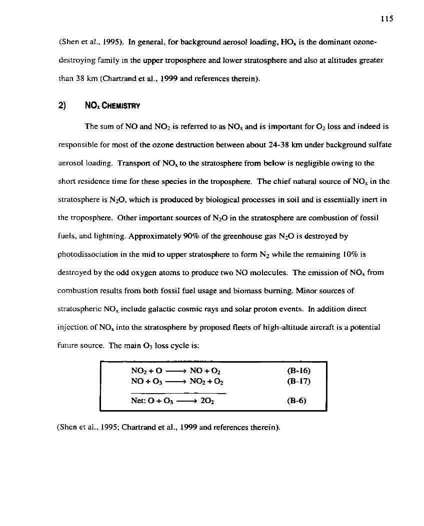
(Shen et al., 1995). In general, for background aerosol loading, HO, is the dominant ozone-
destroying famiiy in the upper troposphere and lower stratosphere and also at altitudes greater
than 38 km (Chartrand et ai., 1999 and references therein).
The sum of NO and NOt is referred to as NO, and is important for O3 IOSS and indeed is
responsible for most of the ozone destruction between about 24-38 km under background sulfate
aerosol loading. Transport of NOx to the stratosphere from below is negligible owing to the
short residence time for these species in the troposphere. The chief natural source of NO, in the
stratosphere is NzO, which is produced by biologicai processes in soi1 and is essentially inert in
the troposphere. Other important sources of NzO in the stratosphere are combustion of fossil
fuels, and lightning. Approximately 90% of the greenhouse gas NzO is destroyed by
photodissociation in the mid to upper stratosphere to forrn Nt while the remaining 10% is
destr~yed by the odd oxygen atoms to produce two NO molecules. The emission of NO, from
combustion results from both fossil fuel usage and biomass burning. Minor sources of
stratospheric NO, include galactic cosmic rays and solar proton events. In addition direct
injection of NO, into the stratosphere by proposed fleets of high-altitude aircraft is a potential
future source. The main Oj IOSS cycle is:
Net: O + O3 + 202
(Shen et al., 1995; Chartrand et al., 1999 and references therein).
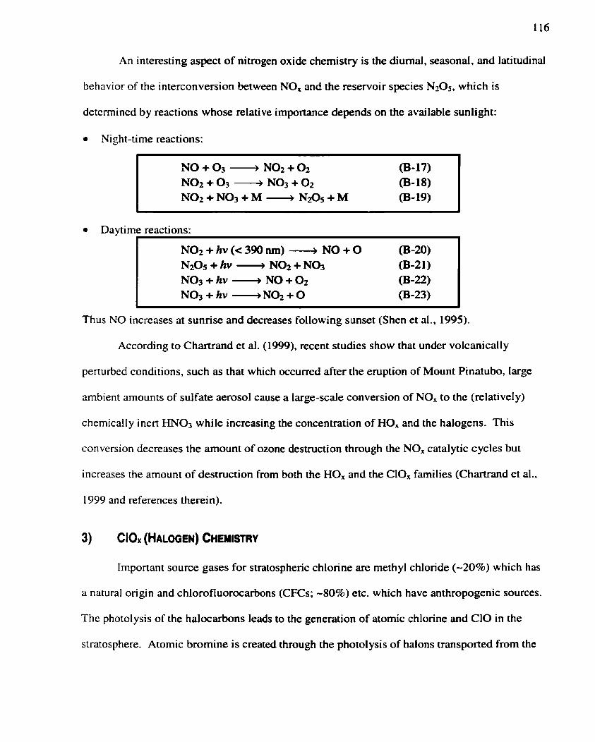
An interesting aspect of nitrogen oxide chemistry is the diurnal, seasonal, and latitudinal
behavior of the interconversion between NO, and the reservoir species N205, which is
determined by reactions whose relative importance depends on the available sunlight:
Night-time reactions:
Davtirne reactions:
Thus NO increases at sunrise and decreases following sunset (Shen et al., 1995).
According to Chartrand et al. (1999), recent studies show that under volcanically
perturbed conditions, such as that which occumed &ter the eruption of Mount Pinatubo, large
ambient amounts of sulfate aerosol cause a large-scale conversion of NOs to the (relatively)
chemically inert HN03 while increasing the concentration of HOs and the halogens. This
conversion decreases the arnount of ozone destruction through the NOs catalytic cycles but
increases the arnount of destruction from both the HO, and the CIO, families (Chartrand et al.,
1999 and references therein).
Important source gases for stratospheric chlorine are methyl chloride (-20%) which has
ri natura! origin and chlorofluorocarbons (CFCs; -80%) etc. which have anthropogenic sources.
The photolysis of the halocarbons leads to the generation of atomic chlorine and C l0 in the
stratosphere. Atomic bromine is created through the photo1 ysis of halons transported from the

troposphere and through the destruction of CH3Br. Although the mixing ratio of bromine is
small. it can contnbute, as much as 30% to the total ozone loss during formation of the Antarctic
ozone hole. Interaction with ozone results in catalytic cycles such as:
Net: O + 0 3 + 202 And
B r + 0 3 + BrO+02 BrO+O --+ B r + 0 2
Net: O + O3 + 202 Or the sequence
Cl + O3 + CIO + O2 2C10 + Cl2 + o2 Cl2 + hv --+ Cl + Cl
Net: 203 + 302 And
B r + 0 3 + BrO+02 CI + o3 + CIO + o2 BrO + Cl0 --4 BrCl + 0 2
BtCl+hv + Br+Cl
(Chartrand et al.. 1999).
CFCs are used as refngerants, solvents, aerosol propellants, and blowing agents for
plastic foams. These chemicals are very inert: they have no tropospheric sinks and are not
water-soluble, and thus are mixed rapidly throughout the troposphere and gradualiy through the
stratosphere, where eventually they photodissociate. CFCs need not rise above most of the
atmospheric O2 and 03, because they cm be photodissociated by wavelengths which penetrate
to lower altitudes, in the 185-210 nm spectral window. As examples consider the two rnost
prominent CFCs that reach the stratosphere, CFC- 1 1 (CFC13) and CFC-12 (CF2Cli):

Subsequent reactions of the CFClz and CFzCl radicals lead to the rapid release of the remaining
chlonne atoms, which then initiate the catalytic cycles (Shen et al., 1995).
4) COUPLING OF HOJNOXIOr REACTIONS
The importance of a farnily of species and its cycles depends on the abundance of the
active radicaIs that initiate the chah reactions, which in turn depends on the amount held in
reservoir form and the likelihood of radical regeneration. The segregation of reactions of
various species into individual catalytic cycles is a useful tool for understanding the nature of
the ozone destruction processes. Note, however, that the choice of the cycles is arbitrary: the
concentration of any given species is dependent on al1 the reactions in which it participates. An
important set of resictions is the coupling of the different radical families. The most important
reactions coupling HO, and NO, are:
Reaction (B-34) strongly affects the partitioning of OH and HO?, and hence the relative
contributions of the various HO, catalytic cycles (Shen et al., 1995).
The effectiveness of the NOx cycIe is reduced when NOz is tied-up through reaction (B-
35), a key reaction coupling the HOx and NO,cycles. Reaction (B-37) also ties-up NO?. The
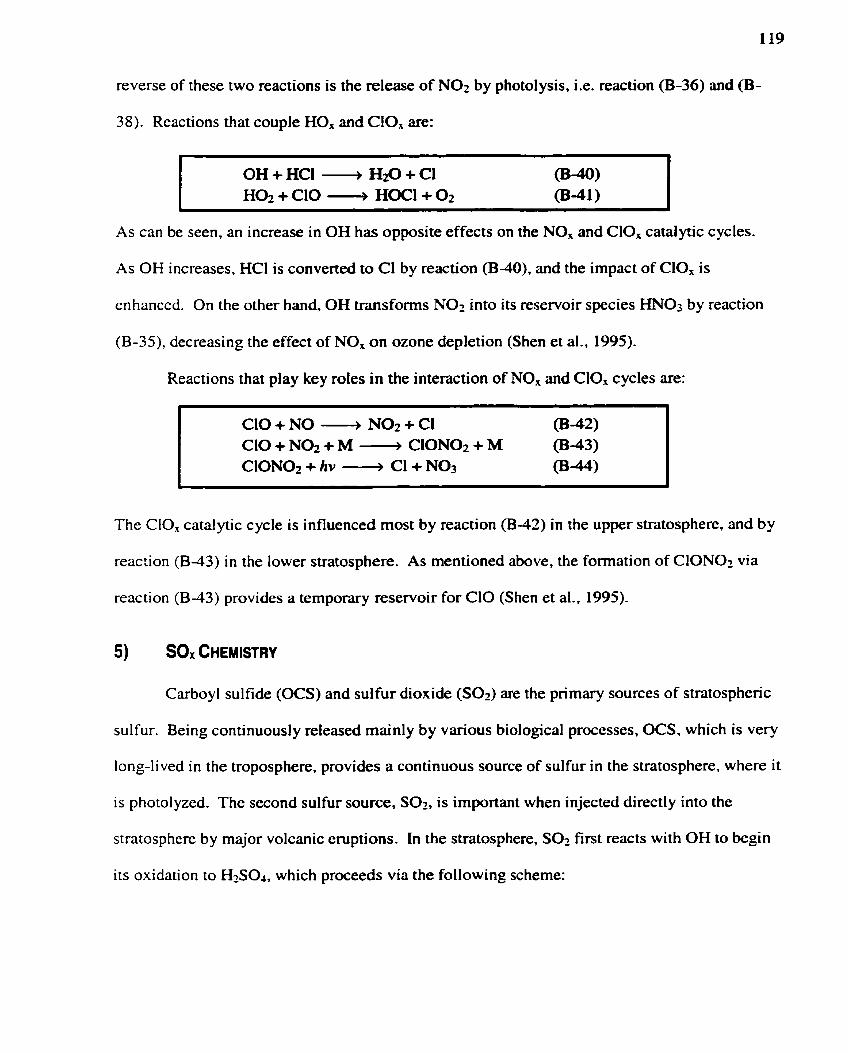
reverse of these two reactions is the release of NOz by photolysis, i.e. reaction (B-36) and (B-
38). Reactions that couple HO, and CIO, are:
- -
OH + HCI + H20 + Cl
As can be seen, an increase in OH has opposite effects on the NOx and CIO, catalytic cycles.
As OH increases, HCI is converted to Cl by reaction (B-40), and the impact of CIO, is
enhanced. On the other hand, OH transforrns NO2 into its reservoir species KN03 by reaction
(B-35), decreasing the effect of NO, on ozone depletion (Shen et al., 1995).
Reactions that play key rotes in the interaction of NO, and CIO, cycles are:
The CIO, catalytic cycle is influenced most by reaction (B-42) in the upper stratosphere, and by
reaction (B-43) in the lower stratosphere. As rnentioned above, the formation of ClONOz via
reaction (B-43) provides a temporary resewoir for CIO (Shen et al., 1995).
5)
sulfur
long-1
Carboyl sulfide (OCS) and suifur dioxide (SOz) are the primary sources of stratosphenc
,. Being continuously reieased mainly by various biological processes, OCS, which is very
ived in t h e troposphere, provides a continuous source of sulfur in the stratosphere, where it
is photolyzed. The second suifur source, SOz, is important when injected directly into the
stratosphere by major volcanic eruptions. In the stratosphere, SOz first reacts with OH to b e n
its oxidation to H2S04, which proceeds via the following scheme:

Note that no HO, radicals are consumed in this process. The extremely hygroscopic
product, H2S04, combines with water vapor to form sulfate aerosol particles, which play a major
roIe in stratospheric chemistry by providing surface for heterogeneous reactions as well as by
being involved in the formation of polar stratosphere clouds. These play a crucial role in the
near complete seasonal destruction of ozone which occurs over Antarctica (Shen et al., 1995 and
references therein).
6) HIGH-LATITUDE OZONE LOSS AND HETEROGENEOUS CHEMISTRY
Reactions that occur odin a condensed phase such as a liquid andor a solid are known
col lecti vel y as heterogeneous reactions. Small condensation nuclei can form in the troposphere
and stratosphere by homogeneous nucleation, and these nuclei in turn can grow by condensation
and coagulation or by heterogeneous nucleation. Once formed, these aerosol particles can act as
surfaces upon which reactions can proceed; reactions that are normally kinetically limited in the
gas phase (Chartrand et al., 1999).
This mechanism means that a pseudo-liquid aerosol surface is not required in order for
effective HCI uptake to occur just an ice surface. The rate of a reaction of this type will be
dependent on surface area but it is possible that there will be significant diffusion of the
adsorbed/absorbed species into the aerosol. In this case, the rate of the reaction wilI be
proportional to the available aerosol volume. Generally, there are two major types of surfaces:
(1) sulfate aerosols and (2) polar stratospheric clouds (PSCs), each of which will be discussed
separately below (Chartrand et al., 1999 and references therein).
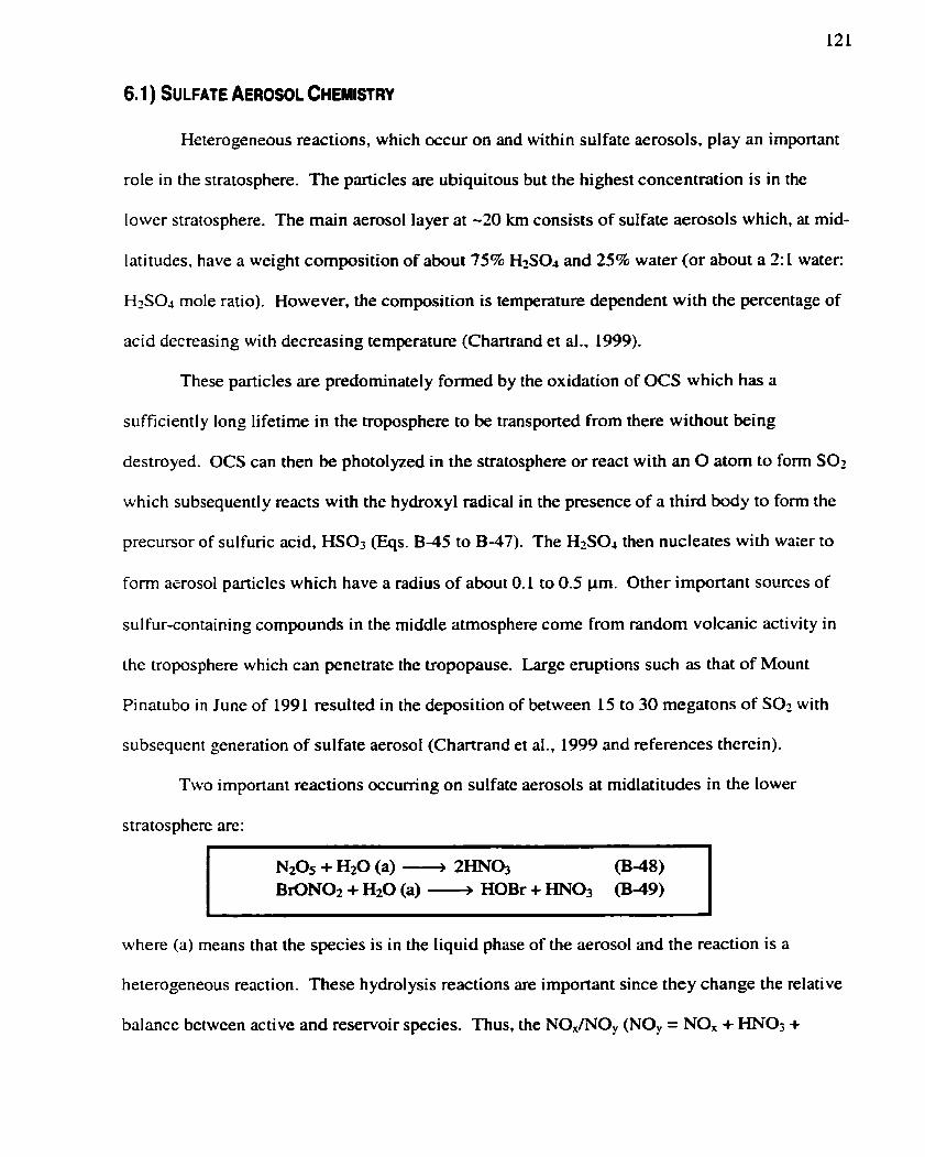
Heterogeneous reactions, which occur on and within sulfate aerosols, play an important
role in the stratosphere. The particles are ubiquitous but the highest concentration is in the
lower stratosphere. The main aerosol layer at -20 km consists of sulfate aerosols which, at rnid-
latitudes, have a weight composition of about 75% H2S04 and 25% water (or about a 1: 1 water:
HISOj mole ratio). However, the composition is temperature dependent with the percentage of
acid decreasing with decreasing temperature (Chartrand et al., 1999).
These particles are predorninately formed by the oxidation of OCS which has a
sufficiently long lifetime in the troposphere to be transported from there without k ing
destroyed. OCS can then be photolyzed in the stratosphere or react with an O atom to form SOI
which subsequently reacts with the hydroxyl radical in the presence of a third body to fom the
precursor of sulfuric acid, HS03 (Eqs. B-45 to B-47). The HzSOJ then nucleates with waîer to
fonn asrosol particles which have a radius of about 0.1 to 0.5 Pm. Other important sources of
sulfur-containing compounds in the middle atmosphere come from random volcanic activity in
the troposphere which can penetrate the tropopause. Large eruptions such as that of Mount
Pinatubo in June of 1991 resulted in the deposition of between 15 to 30 megatons of SOz with
su bsequent generation of sulfate aerosol (Chartrand et al., 1999 and references therein).
Two important reactions occumng on sulfate aerosols at midlatitudes in the lower
stratosphere are:
N20s + H20 (a) - 2HN03 (B-48) BrONOz + H20 (a) --+ HOBr + HN03 (B-49)
where (a) means that the species is in the Iiquid phase of the aerosol and the reaction is a
heterogeneous reaction. These hydrolysis reactions are important since they change the relative
balance between active and reservoir species. Thus, the NOx/NO, (NO, = NO, + HNO3 +

HNO? + . . .) ratio may decrease due to conversion of NzOs and BrON02 to HN03. However,
while the nitrogen-cycle ozone losses may decrease, ozone loss due to HOx and CIO, may
increase. Active chlonne species wilI increase because the reduction in NO- will result in less
CIO being present as CIONOr, a chlorine reservoir species. Odd hydrogen will also increase
due to the photolysis of HOBr and HN03 via:
HOBr + hv + O H + Br (B-50) HN03 + hv ---+ OH + NOz (B-51)
F
The enhanced OH and HOz will increase ozone destruction through the HOx catalytic cycles. In
addition, the increased OH will also release Cl from HCI, another reservoir species through the
following reaction:
The above reaction also results in increased CIO levels (Chartrand et aI., 1999 and references
therein).
Another reaction that becornes important when the temperature decreases below about
205 K is:
CION02 + HzO (a) + HOC1 + HNO3 (B-53)
This reaction is expected to become important at higher latitudes where temperatures are
generally lower or under volcanically induced conditions (Chartrand et al., 1999).
6.2) POLAR STRATOSPHERIC CLOUD CHEMISTRY
When the atmosphere cools below the water ice frost point (-188 K), PSCs made of ice
c m form. Other PSCs made of H2SOdHN03/H20 or nitric acid trihydrate (HN03.3Hz0 or
NAT) are also able to nucleate and freeze after ice is formed. Heterogeneous reactions on these
condensed phases can activate chlonne and bromine with odd nitrogen as HN03 (a). The active

chlorine and, to a lesser extent, brornine drive the reactions that forrn the ozone hole. For
example, on the ice crystals, inactive or reservoir foms of the halogen catalysts are freed
through the following reactions:
Cl0NO2 + HX (US) ---+ HN03(L/s) + XCl ( g s ) (B-54) N2O5 + HX (fi) + HN03(L/s) + XNO2 (gas) (B-55)
where (Us) means the species remains idon the ice surface or dissolved within the aerosol
solution and where X = Cl, Br (Chartrand et al., 1999 and references within).
Low temperatures are crucial to this prwess. As the polar lower stratospheric
temperatures decrease at the end of the fall season, these PSC reactions become important. For
example, the solubility of HCI is very temperature dependent, and as the temperature drops, HCI
begins to dissolve in sulfate aerosol. These and similar reactions initiate the large decrease in
ozone in late polar winter (Noïthem Hemisphere) and Antarctic springtime (Chartrand et al.,
These reactions can occur during the night-tirne and, when polar sunrise occurs, species
such as Cl?, BrCl and CINOz are readily photolyzed into species such as Cl and Cl0 which then
can participate in ozone destroying catalytic cycles. In the austral vortex, CIO concentrations
after polar sunnse can reach about 1 ppbv or more, two orders of magnitude large than those
typically found in the midlatitude stratosphere (Chartrand et al., 1999 and references therein).
One of the main features of ozone loss in polar regions is that it is not rate limited by the
low abundance of atomic oxygen. One of the main loss mechanisms involves self-reaction of
C l0 + Cl0 + M + C1202 + M 03-56) C1202 + hv + CI + Cl02 03-57] C102+M + C 1 + 0 2 + M (B-58) 2 x (CI +O2 + CiO+02) 03-59)
Net: O3 + O3 ---+ 3 0 2 03-60)

124
In this case the ozone loss rate is proportional to [CIO]'. Thus as more CIO, is converted to
CIO, the rate of ozone destruction is quadratic with respect to active CIO, (Chartrand et al.,
1999 and references therein).
Another important ozone loss mechanism is due to the synergistic reaction between B r 0
and CIO:
As before, this loss is not lirnited by the abundance of atornic oxygen. A major product of the
reaction between Br0 and CIO is OC10 which in fact leads to a null cycle (no odd oxygen is
destroyed). This is because OC10 in the presence of sunlight rapidly dissociates to Cl0 and O
(odd oxygen). At 190 K, approximately 60% of Br0 and Cl0 reactions result in a null cycle,
whiIe approxirnâtely 36% fom Br and Cl00 (which photolyse to CI and O?). The remaining
-4% foms the BrCl molecule (which is photolytic) and motecular oxygen (Chartrand et al.,
1999 and references therein).