in highway crashes a dissertation submitted to the faculty
TRANSCRIPT
FINITE ELEMENT MODELING AND SIMULATION OF OCCUPANT RESPONSES
IN HIGHWAY CRASHES
by
Ning Li
A dissertation submitted to the faculty of
The University of North Carolina at Charlotte
in partial fulfillment of the requirements
for the degree of Doctor of Philosophy in
Mechanical Engineering
Charlotte
2014
Approved by:
______________________________
Dr. Howie Fang
______________________________
Dr. David C. Weggel
______________________________
Dr. Harish P. Cherukuri
______________________________
Dr. Ronald E. Smelser
______________________________
Dr. Don Chen

ii
© 2014
Ning Li
ALL RIGHTS RESERVED

iii
ABSTRACT
NING LI. Finite element modeling and simulation of occupant responses in highway
crashes. (Under the direction of DR. HOWIE FANG)
Roadside barrier systems play an important role in reducing the number of
fatalities and the severity of injuries in highway crashes. After decades of work by
researchers and engineers, roadside barriers have been improved and are generally
effective in preventing head-on collisions and thus crash fatalities. To further improve the
performance of highway safety devices and develop new systems, a good understanding
of occupant injuries is required. Although incorporating occupant responses and/or
injuries into the design of safety devices is highly recommended by the current safety
regulations, there are currently no studies that can be used to develop official guidelines
or standards. Despite its usefulness in understanding the crash mechanism and improving
vehicle crashworthiness, crash testing is very expensive and restricted by the crash
scenarios that can be investigated. In addition, no crash test dummy is incorporated in
majority of the crash testing of roadside barriers.
With the recent advances in high performance computing and numerical codes,
computer modeling and simulation are playing an important role in crash analysis and
roadside safety research. In this study, the finite element model of a Hybrid III 50th
percentile male dummy was developed for studying the driver’s responses in vehicular
crashes into highway barriers. After validation by standard crash tests, the dummy model
was combined with the finite element model of a 2006 Ford F250 pickup truck and used
in simulations of the vehicle impacting a concrete barrier and a W-beam guiderail under
different impact speeds and angles. Finally, the dummy responses in these simulations

iv
were analyzed by correlating with existing human injury criteria so as to correlate impact
severity to vehicular responses and ultimately to barrier performances.
v
ACKNOWLEDGEMENTS
Writing of this dissertation has been one of the most significant challenges I have
ever faced. Without the supports, kindness and encouragements of many people, this
study would not have been completed.
I would like to express my deepest gratitude to my advisor, Dr. Howie Fang, for
his caring, patience, support, believing in me and guiding me during the course of my
research work. Without the help of Dr. Fang, this dissertation would not have been
possible.
I would also like to thank Dr. David C. Weggel, Dr. Harish P. Cherukuri, Dr.
Ronald E. Smelser and Dr. Don Chen to be my committee members with their valuable
time, reviews, comments and advice on my dissertation.
Special thanks go to Tracy L. Beauregard for kindness and excellent student
service; to my colleagues, Jing Bi, Matthew DiSogra, Matthew Gutowski, Ning Tian, and
Xuchun Ren; to the University Research Computing staff, Jonathan Halter and Charles E.
Price.
Lastly but not the least, I would like to thank my parents and my aunt who have
always encouraged, supported and believed in me. Thank Anna Ye for kindness and
encouragements.
vi
TABLE OF CONTENTS
CHAPTER 1: INTRODUCTION 1
1.1 Vehicular Crashworthiness and Roadside Safety 1
1.2 Traffic Barrier Design and Crash Testing 9
1.3 Occupant Injuries 14
1.4 Finite Element Modeling of Crash Problems 20
CHAPTER 2: CONTACT ANALYSIS 36
2.1 Numerical Implementations of Contact Theories 36
2.2 Contact Modeling in LS-DYNA 50
CHAPTER 3: FINITE ELEMENT MODELING OF VEHICLES 60
3.1 FE Model of a 2006 Ford F250 Pickup Truck 65
3.2 FE Model of the Passive Restraint System 87
CHAPTER 4: FINITE ELEMENT MODELING OF A HYBRID-III DUMMY 96
4.1 Finite Element Modeling of Crash Dummies 98
4.2 The LSTC_NCAC Dummy Model 106
4.3 Development of a Hybrid-III Dummy Model for Roadside Crash Simulations 115
4.4 Validation of the Revised Dummy Model: ISOL Dummy Model 119
CHAPTER 5: FINITE ELEMENT MODELING AND SIMULATION OF 145
HIGHWAY CRASHES
5.1 FE Modeling of Median Barriers 148
5.2 Vehicular Crash into a New Jersey Concrete Median Barrier 149
5.3 Vehicular Crash into a W-beam Guardrail 163
CHAPTER 6: ANALYSIS OF OCCUPANT INJURIES IN HIGHWAY CRASHES 177
6.1 Occupants Injuries and Injury Criteria 177

vii
6.2 Occupants Injuries Evaluation using Vehicle Responses 182
6.3 Occupants Injuries Evaluation using Crash Test Dummy 191
6.4 Correlation between Vehicle Responses and Occupant Injuries 194
CHAPTER 7: CONCLUSIONS 205
REFERENCES 209
CHAPTER 1: INTRODUCTION
Transportation safety or roadside safety refers to the protection of motorists,
cyclists, and pedestrians by roadway hardware systems in any kind of collisions.
According to the World Health Organization (WHO), there are approximately 1.2 million
people died in roadway crashes and millions injured each year (WHO 2013). According
to the National Highway Traffic Safety Administration (NHTSA), there were 32,367
people killed and 2.22 million people injured in the U.S. in 2011 from 5,338,000 reported
motor vehicle crashes (NHTSA 2013). The death tolls are much higher in some
developing countries such as India and China. Consequences of traffic accidents are
severe, because they involve individual life losses, property damages, individual financial
burden, social economic losses and burdens, and long term psychological sufferings.
With long recognized significance, roadside safety has been the concerns of both
researchers and the general public for decades. Numerous programs and research efforts
are devoted to better understand crash mechanism and ultimately, prevent catastrophic
automobile collisions and improve transportation safety.
1.1 Vehicular Crashworthiness and Roadside Safety
Real world automobile accidents occur when a vehicle collides with another
vehicle or a stationary object such as a tree, light pole, or median barrier. Analysis of
real-world crash data and the use of simulation codes help better understand the nature
and severity of roadside crashes and develop designs with improved safety.

2
Research on real world vehicle collisions is very challenging since most of the
crash events are unpredictable and unrepeatable with few real-time crash data being
recorded. As a result, researchers often turn to well defined laboratory tests, such as full-
frontal impact, offset frontal impact, side impact, rear impact, and rollover test to
examine the vehicle’s crashworthiness performances. Instruments and recording devices
are installed before a test so that real-time data can be gathered and analyzed. More
importantly, the ability of vehicular structures to protect the occupants during collisions
is examined by the collected test data. For example, the deformations of the vehicle
structures and accelerations at different locations (including those on the crash test
dummies) can be measured and used to predict the injury probability and/or severity
caused to the occupants.
The above mentioned procedures are referred as vehicle crashworthiness analysis,
which focuses on the ability of a vehicle to absorb the crash energy with controlled level
of deformations and to prevent significant amount of loads from being transferred to the
occupants (through the use of restraint systems). The energy absorption is primarily
accomplished by plastic deformations and fractures. The restraint system distributes the
sharp impact loads from vehicle structures to a larger time frame and reduces the
peak/maximum impact force and acceleration experienced by the occupants.
Despite their limited crash scenarios, laboratory tests are not isolated from real
world crash events and have their roots in real world applications. For example,
approximately half of the occupants killed in passenger vehicles in the U.S. are from
frontal crashes. Major improvements on safety equipment such as seatbelts and airbags
for frontal crash protection are largely attributed to the full-frontal impact test initiated by
3
the New Car Assessment Program (NCAP) in 1978 by NHTSA as well as the offset
frontal impact test by the Insurance Institute for Highway Safety's (IIHS) in 1995. Today,
all vehicles in the U.S. market are required to meet the safety requirements by the Federal
Motor Vehicle Safety Standards (FMVSS) No. 208 (NHTSA 1998) which defines and
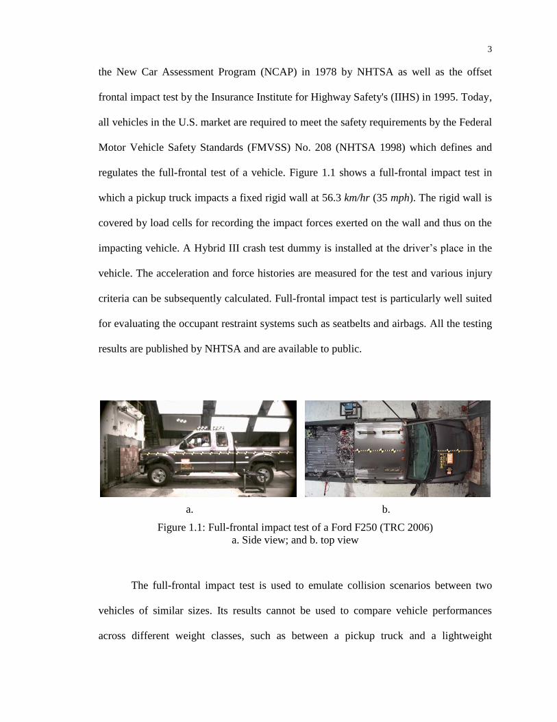
regulates the full-frontal test of a vehicle. Figure 1.1 shows a full-frontal impact test in
which a pickup truck impacts a fixed rigid wall at 56.3 km/hr (35 mph). The rigid wall is
covered by load cells for recording the impact forces exerted on the wall and thus on the
impacting vehicle. A Hybrid III crash test dummy is installed at the driver’s place in the
vehicle. The acceleration and force histories are measured for the test and various injury
criteria can be subsequently calculated. Full-frontal impact test is particularly well suited
for evaluating the occupant restraint systems such as seatbelts and airbags. All the testing
results are published by NHTSA and are available to public.
a. b.
Figure 1.1: Full-frontal impact test of a Ford F250 (TRC 2006)
a. Side view; and b. top view
The full-frontal impact test is used to emulate collision scenarios between two
vehicles of similar sizes. Its results cannot be used to compare vehicle performances
across different weight classes, such as between a pickup truck and a lightweight

4
passenger car. Since the kinetic energy of the vehicle depends on its speed and weight, a
heavier vehicle crashing at the same impact speed results in more severe damages than a
lighter vehicle due to the former’s larger amount of kinetic energy. On the other hand, a
small passenger car that is considered safe in a frontal impact test may not be considered
safe when colliding with a heavy truck as illustrated by the situation in Figure 1.2.
Figure 1.2: A highway crash of a small passenger car and a tractor trailer (URL1)
Besides full-frontal impact tests, additional information regarding vehicle
deformations and occupant safety can be obtained by offset frontal impact tests. Unlike
full-frontal impact tests, offset frontal tests focus more on the vehicle’s structural
performances. Recent testing performed by the International NCAP Agencies showed
that full-frontal crash tests do not show how effective a vehicle's safety cabin and the
occupant restraint system will protect the occupants in a real world collision. Real world
collisions are often far off from the ideal head-on collisions and the vehicle’s structural
damages are usually more severe in some local regions than in full-frontal impacts. Since
a frontal impact test does not evaluate the vehicle’s structural damages, it is possible for a
vehicle to have a poorly performed compartment even though it passes the NHTSA test
based on head and chest injury criteria.
5
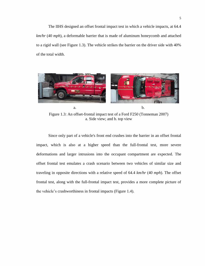
The IIHS designed an offset frontal impact test in which a vehicle impacts, at 64.4
km/hr (40 mph), a deformable barrier that is made of aluminum honeycomb and attached
to a rigid wall (see Figure 1.3). The vehicle strikes the barrier on the driver side with 40%
of the total width.
a. b.
Figure 1.3: An offset-frontal impact test of a Ford F250 (Tonneman 2007)
a. Side view; and b. top view
Since only part of a vehicle's front end crushes into the barrier in an offset frontal
impact, which is also at a higher speed than the full-frontal test, more severe
deformations and larger intrusions into the occupant compartment are expected. The
offset frontal test emulates a crash scenario between two vehicles of similar size and
traveling in opposite directions with a relative speed of 64.4 km/hr (40 mph). The offset
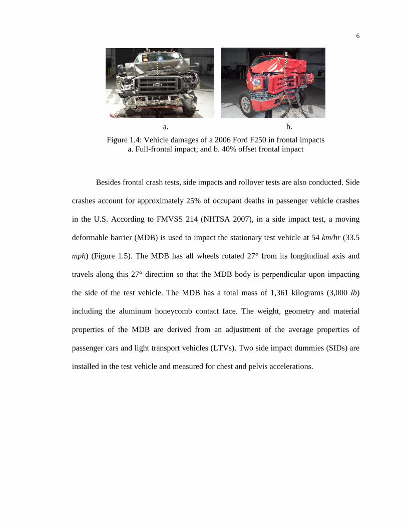
frontal test, along with the full-frontal impact test, provides a more complete picture of
the vehicle’s crashworthiness in frontal impacts (Figure 1.4).
6
a. b.
Figure 1.4: Vehicle damages of a 2006 Ford F250 in frontal impacts
a. Full-frontal impact; and b. 40% offset frontal impact
Besides frontal crash tests, side impacts and rollover tests are also conducted. Side
crashes account for approximately 25% of occupant deaths in passenger vehicle crashes
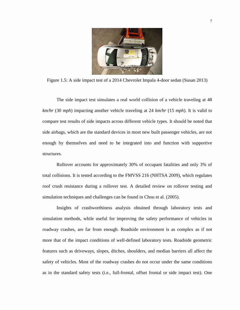
in the U.S. According to FMVSS 214 (NHTSA 2007), in a side impact test, a moving
deformable barrier (MDB) is used to impact the stationary test vehicle at 54 km/hr (33.5
mph) (Figure 1.5). The MDB has all wheels rotated 27° from its longitudinal axis and
travels along this 27° direction so that the MDB body is perpendicular upon impacting
the side of the test vehicle. The MDB has a total mass of 1,361 kilograms (3,000 lb)
including the aluminum honeycomb contact face. The weight, geometry and material
properties of the MDB are derived from an adjustment of the average properties of
passenger cars and light transport vehicles (LTVs). Two side impact dummies (SIDs) are
installed in the test vehicle and measured for chest and pelvis accelerations.
7
Figure 1.5: A side impact test of a 2014 Chevrolet Impala 4-door sedan (Susan 2013)
The side impact test simulates a real world collision of a vehicle traveling at 48
km/hr (30 mph) impacting another vehicle traveling at 24 km/hr (15 mph). It is valid to
compare test results of side impacts across different vehicle types. It should be noted that
side airbags, which are the standard devices in most new built passenger vehicles, are not
enough by themselves and need to be integrated into and function with supportive
structures.
Rollover accounts for approximately 30% of occupant fatalities and only 3% of
total collisions. It is tested according to the FMVSS 216 (NHTSA 2009), which regulates
roof crush resistance during a rollover test. A detailed review on rollover testing and
simulation techniques and challenges can be found in Chou et al. (2005).
Insights of crashworthiness analysis obtained through laboratory tests and
simulation methods, while useful for improving the safety performance of vehicles in
roadway crashes, are far from enough. Roadside environment is as complex as if not
more that of the impact conditions of well-defined laboratory tests. Roadside geometric
features such as driveways, slopes, ditches, shoulders, and median barriers all affect the
safety of vehicles. Most of the roadway crashes do not occur under the same conditions
as in the standard safety tests (i.e., full-frontal, offset frontal or side impact test). One

8
type of roadway crashes, the so-called “roadway departure crashes,” is typically severe
and accounts for the majority of highway fatalities. This type of crashes occurs when a
driver runs off the road and hits obstacles such as a tree, a light pole, another car or other
fixed objects. According to the Roadway Departure Safety Program of the U.S.
Department of Transportation, there were 15,307 fatal roadway departure crashes in 2011,
which resulted in 16,948 fatalities or 51% of the total fatal crashes in the U.S.
Among roadway departure crashes, head-on collisions have been a major source
of severe injuries and fatalities. Head-on collisions are crashes of two vehicles traveling
in direct opposition and thus are the most severe crashes. Head-on collisions have a 3%
fatality rate and close to 100% injury rate (NHTSA 2013). In 2011, 2,731 fatal head-on
collisions account for 0.5 percent of 5,338,000 total crashes but responsible for 9.2% of
29,757 total fatal crashes (NHTSA 2013). Since head-on collisions on highways usually
occur when vehicles cross the median and strike another vehicles in the opposing traffic,
installing median barrier is necessary to prevent vehicles from crossing the median so as
to avoid head-on collisions (Figure 1.6). Median barriers are especially effective in
reducing the chances of small, light passenger vehicles crashing into large, heavy
vehicles.
9
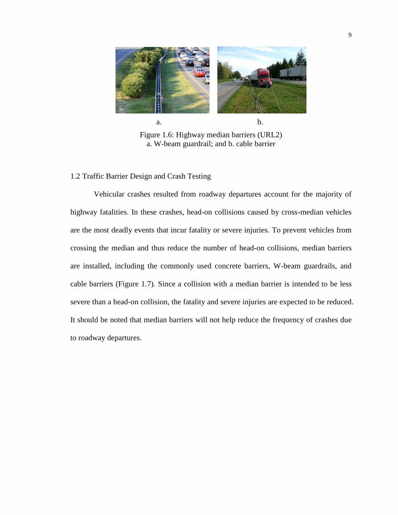
a. b.
Figure 1.6: Highway median barriers (URL2)
a. W-beam guardrail; and b. cable barrier
1.2 Traffic Barrier Design and Crash Testing
Vehicular crashes resulted from roadway departures account for the majority of
highway fatalities. In these crashes, head-on collisions caused by cross-median vehicles
are the most deadly events that incur fatality or severe injuries. To prevent vehicles from
crossing the median and thus reduce the number of head-on collisions, median barriers
are installed, including the commonly used concrete barriers, W-beam guardrails, and
cable barriers (Figure 1.7). Since a collision with a median barrier is intended to be less
severe than a head-on collision, the fatality and severe injuries are expected to be reduced.
It should be noted that median barriers will not help reduce the frequency of crashes due
to roadway departures.

10
a. b. c.
Figure 1.7: Commonly used traffic median barriers
a. Concrete barrier; b. W-beam barrier; and c. cable barrier
The practice of installing and developing concrete barriers on highways started
from the early 1940s, according to NCHRP Synthesis 244 (Ray and McGinnis 1997).
Based on observations of accidents on their installed concrete barriers, the state DOT of
New Jersey designed the barrier shapes with two major considerations: (1) the vehicle
needs to be redirected; and (2) the vehicle rollover should be prevented from riding up
the slope on the impacting side of the barrier. The New Jersey barrier, which is
commonly referred to as ‘Jersey barrier,’ has been widely used since its inception and a
few different designs of the concrete barriers were also proposed. Figure 1.8 shows the
cross section of a Jersey barrier compared to an F-shape barrier and a constant slope
barrier.
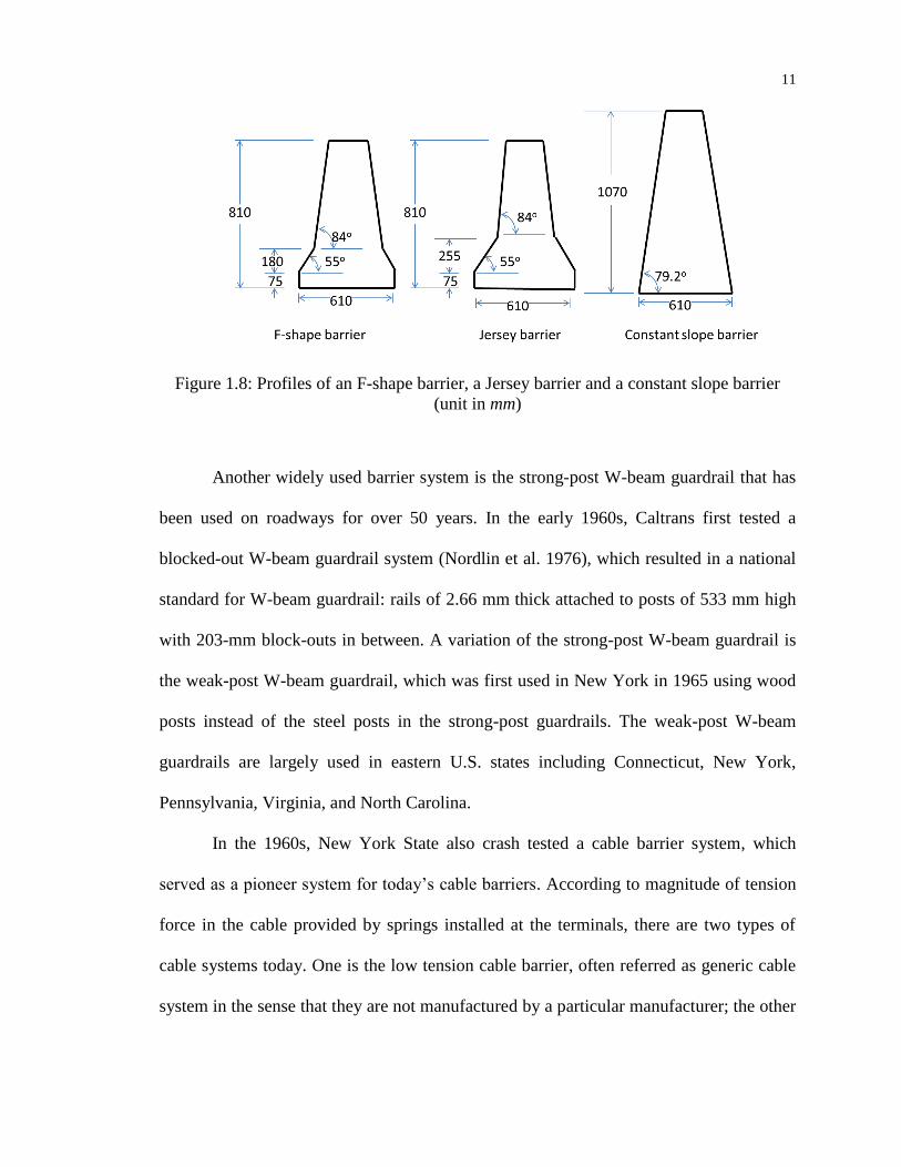
11
Figure 1.8: Profiles of an F-shape barrier, a Jersey barrier and a constant slope barrier
(unit in mm)
Another widely used barrier system is the strong-post W-beam guardrail that has
been used on roadways for over 50 years. In the early 1960s, Caltrans first tested a
blocked-out W-beam guardrail system (Nordlin et al. 1976), which resulted in a national
standard for W-beam guardrail: rails of 2.66 mm thick attached to posts of 533 mm high
with 203-mm block-outs in between. A variation of the strong-post W-beam guardrail is
the weak-post W-beam guardrail, which was first used in New York in 1965 using wood
posts instead of the steel posts in the strong-post guardrails. The weak-post W-beam
guardrails are largely used in eastern U.S. states including Connecticut, New York,
Pennsylvania, Virginia, and North Carolina.
In the 1960s, New York State also crash tested a cable barrier system, which
served as a pioneer system for today’s cable barriers. According to magnitude of tension
force in the cable provided by springs installed at the terminals, there are two types of
cable systems today. One is the low tension cable barrier, often referred as generic cable
system in the sense that they are not manufactured by a particular manufacturer; the other

12
one is the proprietary high tension cable barrier, i.e. all of them exclusively owned by
private companies.
Median barriers, depending on the stiffness, are generally characterized into three
categories: rigid (e.g., concrete barriers), semi-rigid (e.g., W-beam guardrails) and
flexible (e.g., cable barriers). Each of these barrier systems has its own advantages and
disadvantages. Rigid barriers can effectively reduce median crossovers, especially in
locations with high traffic volumes and/or high speeds and in areas with narrow median
widths. However, rigid barriers do not have large deformation and thus do not absorb
much energy; this will likely result in severe crash injuries or even fatalities. Semi-rigid
barriers offer more flexibility than rigid barriers and thus absorb more energy during a
crash as a result of rail and post deformations in addition to the vehicle’s deformation.
For W-beam guardrails, even a small damage may degrade its performance in a
subsequent crash and thus requires immediate repairs, which increase the maintenance
costs. Flexible barriers such as cable barriers are the most forgiving systems among the
three categories for its large transverse deflection of the cables during a crash. The
resulting contact force on the vehicle is usually much smaller than those by rigid and
semi-rigid barriers. The major drawback is that cable barriers require sufficiently large
median width to accommodate the cables’ transverse deflections. Additionally, small
passenger vehicles may under-ride the cables and cause cross-median collisions.
Full-scale crash testing has been the most common way of evaluating the
performance of barrier systems before their placements on highways. The performance of
a barrier under vehicular impacts is typically assessed by “the risk of injury to the
occupants of the impacting vehicle, the structural adequacy of the safety feature” and “the

13
post-impact behavior of the test vehicle” (Sicking et al. 2009). The occupants should not
experience severe or fatal injuries and a vehicle impacting the barrier should not cross
over the barrier and should stay upright during the course of the impact. Since crash
testing is a complex task involving numerous parameters such as vehicle weight, impact
speed, impact angle, and the critical impact point on the barrier, a crash testing procedure
needs to be carefully planned with consideration of these parameters. To this end,
researchers developed standard test procedures such as the NCHRP Report 350 (Ross et
al. 1993) and its successor, the Manual for Assessing Safety Hardware (Sicking et al.
2009). In Manual for Assessing Safety Hardware (MASH), six levels of crash testing are
defined for longitudinal barriers and each level has a specific impact speed, impact angle,
types of vehicles, and vehicles’ weights. Among the six test levels in MASH, the most
commonly used impact configuration is the one with a vehicle impacting a barrier at an
impact speed of 100 km/hr and an impact angle of 25°, representing the conditions of the
most frequently occurred run-off-road crashes.
It should be noted that the in-service performance of a highway barrier system
cannot be fully measured or determined by a series of standard crash tests (Sicking et al.
2009). Crash testing is necessary but insufficient to demonstrate the performances of a
barrier system under real-life vehicular impacts. The performances of a specific barrier
can be significantly affected by a number of factors such as site conditions, vehicle types
and features, driver’s behaviors, weather conditions, material properties of the barrier
components, and maintenance of the barrier. It is simply infeasible to test all possible
scenarios in the standardized crash tests.

14
1.3 Occupants Injuries
Approximately 1.24 million people die every year on the world’s roads, and
millions sustain nonfatal injuries from vehicular crashes worldwide (WHO 2013).
Understanding human injury in automotive crashes has a significant effect to improving
transportation safety. A key step to study the injury mechanism under automotive crashes
is to determine the mechanical parameters such as loading conditions, stress state, and
strain state that may cause injuries to the human body.
Over the years, a number of injury criteria have been established to estimate the
level of human injury. Medical physicians often use the Abbreviated Injury Scale (AIS)
to quantify the severity of an injury. For example, the level of AIS 1 corresponds to a
minor injury and the level of AIS 5 means a serious life-threatening injury. Research on
injuries of human body on the head, neck, thorax, abdomen, pelvis, and lower extremities
has been conducted in the field of impact biomechanics during the past 60 years (King
2000; 2001). Different parts of the body have different injury mechanisms; injury criteria
for specified body regions have been documented and proposed for assessing the restraint
system in automotive crashes (Eppinger et al. 1999; Kleinberger et al. 1998).
Head injury, which mainly concerns skull fracture and brain injury, is among the
most considered injuries. Although the head skull can safely sustain a relatively large
acceleration within a short period of time, compressive and shear loading due to pressure
gradients may cause pain and damage to the human brain. The head injury criteria (HIC)
based on the head translational accelerations (Versace 1971) was adopted by the U.S.
federal government in the FMVSS 208, which includes the commonly used
criterion. A certain HIC value corresponds to a certain probability of a skull fracture. For
15
example, the probability of a skull fracture associated with an HIC15 of 700 is 31%. No
injury criteria have been established successfully for evaluation of brain injury.
Neck injury usually refers to its spinal cord facture. Injuries of the neck spinal
cord typically result from a combination of axial and bending loads. Currently, there are
no widely accepted criteria established for neck injury due to its geometrical and
structural complexities. In practice the neck could be treated as a slender column or beam
and its axial force and bending moment should be carefully monitored.
Thorax, especially the rib cage and thoracic spine, is critical to protecting the
internal organs. Fracture of the ribs or spines and impact waves could damage those
thorax housed tissues. In automotive crashes, chest compression is largely due to seat belt
loading. According to the Mertz’s injury risk curve for belt restrained occupants (Mertz et
al. 1991), two inches of chest compression in a Hybrid III dummy is associated with 40%
risk of injury and three inches of chest compression is associated with 95% risk of injury.
The FMVSS 208 permits the chest acceleration going beyond 60 g for less than three
milliseconds and a 76 mm chest compression in a frontal crash. Another chest injury
criterion is the thoracic trauma index (Eppinger et al. 1984) based on cadaver tests and
mainly used for side impact safety evaluation; it is defined as half of the sum of the peak
chest acceleration and peal lower spinal acceleration. According to FMVSS 214 the
maximum allowable value of the thoracic trauma index (TTI) is 85 for a four door
vehicle and 90 for a two door vehicle.
Pelvic injury in a frontal impact is usually caused by an impact load on the knee
along the femur bone, resulting in dislocation of the hip. However, available data on
frontal impact is far less in literature than that on side impact. The main reason is that the
16
use of lap belt greatly reduces the number and severity of injuries in frontal crashes
compared to those seen in side crashes. There are currently no criteria established for
evaluating pelvis injuries in frontal impacts by the FMVSS 208. However, the maximum
10-kN load limit required by FMVSS 208 on the femur should provide adequate
protection to the pelvis to avoid injuries. In side impacts, the maximum allowable
acceleration on the pelvis is 130 g according to FMVSS 214.
Injuries of lower extremities, which include legs, knees, ankles, and feet, are often
overlooked since they are most likely not life threatening. However, inconvenience,
physical suffering, and psychological pains can be significant for occupants with severe
extremity injuries. The femur injury criterion in FMVSS 208 which requires the force on
the femur bone is below 10 kN is the only one applicable to lower limb.
1.3.1 Crash Test Dummies and Their Usage in Injury Evaluation
Crash test dummies are full-scale anthropomorphic test devices (ATD) that are
used to simulate human bodies and instrumented to record data of dynamic responses in
vehicular impact testing. Crash test dummies have been used by the automotive industry
for a long time and details of the development of a physical Hybrid III 50th
percentile
male crash dummy in the early days can be found in the work by Backaitis and Mertz
(1994). The effort on developing the hybrid dummies was initiated by the General Motors
Corp. in the 1970s (Foster et al. 1977). From 1971 to 1976, four generations of frontal
impact dummies (FIDs), including Hybrid I (1971), Hybrid II (1972), ATD 502 (1973),
and Hybrid III (1976), were developed at the General Motors Corp. The most important
advancements of Hybrid III compared to its predecessors are its superior biomechanical
17
responses of the neck, thorax, and knees which made it the most popular dummy used
until today.
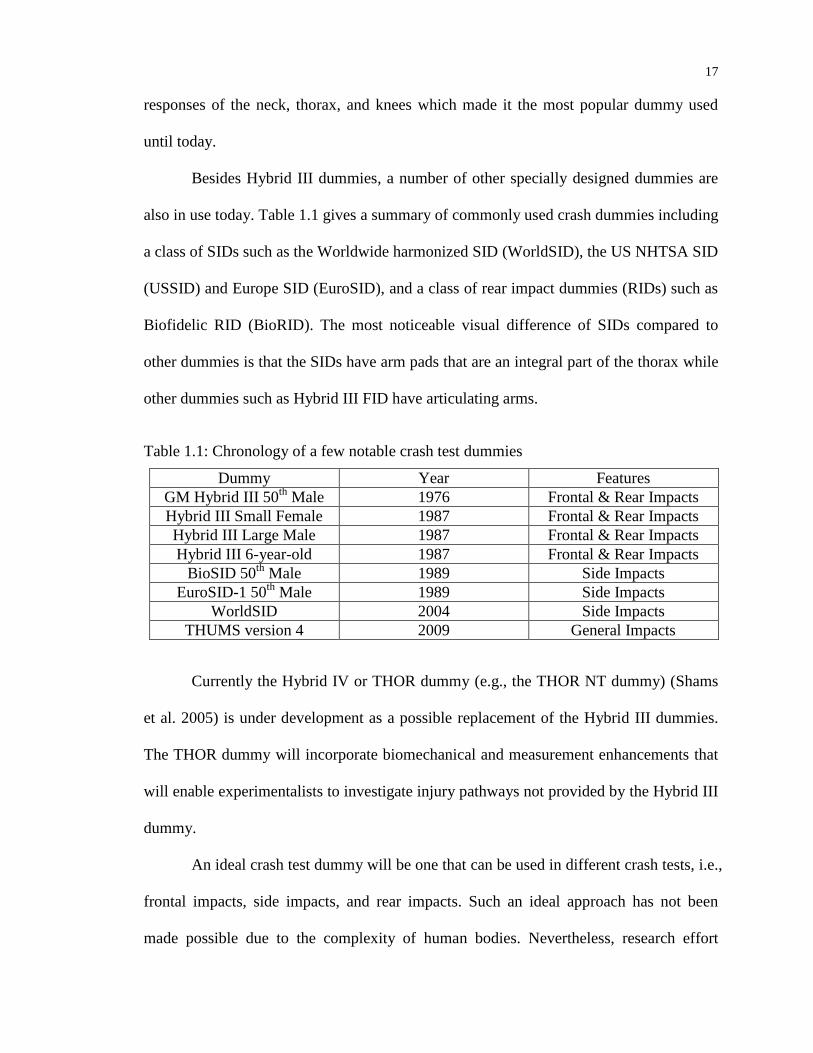
Besides Hybrid III dummies, a number of other specially designed dummies are
also in use today. Table 1.1 gives a summary of commonly used crash dummies including
a class of SIDs such as the Worldwide harmonized SID (WorldSID), the US NHTSA SID
(USSID) and Europe SID (EuroSID), and a class of rear impact dummies (RIDs) such as
Biofidelic RID (BioRID). The most noticeable visual difference of SIDs compared to
other dummies is that the SIDs have arm pads that are an integral part of the thorax while
other dummies such as Hybrid III FID have articulating arms.
Table 1.1: Chronology of a few notable crash test dummies
Dummy Year Features
GM Hybrid III 50th
Male 1976 Frontal & Rear Impacts
Hybrid III Small Female 1987 Frontal & Rear Impacts
Hybrid III Large Male 1987 Frontal & Rear Impacts
Hybrid III 6-year-old 1987 Frontal & Rear Impacts
BioSID 50th
Male 1989 Side Impacts
EuroSID-1 50th
Male 1989 Side Impacts
WorldSID 2004 Side Impacts
THUMS version 4 2009 General Impacts
Currently the Hybrid IV or THOR dummy (e.g., the THOR NT dummy) (Shams
et al. 2005) is under development as a possible replacement of the Hybrid III dummies.
The THOR dummy will incorporate biomechanical and measurement enhancements that
will enable experimentalists to investigate injury pathways not provided by the Hybrid III
dummy.
An ideal crash test dummy will be one that can be used in different crash tests, i.e.,
frontal impacts, side impacts, and rear impacts. Such an ideal approach has not been
made possible due to the complexity of human bodies. Nevertheless, research effort

18
exists on developing a sophisticated computer human model that includes the
complexities and characteristics of flesh, bones, ligaments, blood vessels and organs. One
such example is the Total Human Model for Safety (THUMS) being developed by
TOYOTA as a computational model intended to be highly similar to a real human body
in structures, shapes and materials. No corresponding physical dummy of the THUMS is
produced and validation is accomplished by comparing results of the computer model and
cadaver tests.
No matter what type of dummy model is used, the main purpose is to determine
the potential injuries and/or injury levels (Nyquist et al. 1980); therefore, the use of crash
dummies is necessary for automotive safety because evaluating injuries directly on a
human body is nearly infeasible. The injury levels are determined by analyzing measured
data including the most important injury-related parameters such as acceleration histories
on the head, chest, and pelvis, the forces and moments on the neck, the chest compression,
and forces in the femur bones as well as on the knees.
Since crash test dummies have very good repeatability, they are often used to help
establish the injury criteria that are needed for evaluating the effectiveness of occupant
protection systems in vehicle collisions. These criteria, measured in testing or simulation
studies of crash test dummies and referred as ATD-based injury criteria, are essential to
regulations/laws requiring automobiles to the pass minimum safety requirements before
put into the market. For example, in the US frontal impact regulation FMVSS 208, the
maximum allowable values are set for HIC15 (700), chest acceleration (60 g), and chest
compression (76 mm), and the forces on the femurs (10 kN). In the side impact regulation
FMVSS 214, the maximum allowable pelvis acceleration is set as 130 g.

19
In the field of vehicular crashworthiness, crash test dummies are widely adopted
in both physical crash tests and numerical simulations. Regarding roadway departure
crashes, due to numerous limitations, the current engineering practice only considers the
vehicular behaviors in evaluating the performance of roadside safety barriers. Human
(dummy) models have not been widely adopted for several reasons: 1) there are no
federal regulations that require the usage of dummies and dummy responses in the
evaluation of roadside barrier design, though it is encouraged to do so in the current
safety standard, MASH; 2) currently available dummies, both physical and computer
models, are all not well developed for use in oblique-angle impacts that are typically seen
from traffic barrier crashes. The injury criteria developed for frontal impact and side
impact tests are not quite suitable and may not be directly applied to roadway crashes; 3)
numerical simulations of roadside barrier crashes involving crash dummies are
computationally expensive and challenging due to the requirement of high level
numerical stability of both the vehicle and dummy models.
A thorough understanding and in-depth knowledge of human responses in
roadway crashes involving traffic barriers are indispensable to the successful design of
roadside barrier systems. A link if any between vehicular responses and occupant injuries
would help to simplify the barrier testing procedures and to improve the confidence on
existing barrier systems. Such attempts were shown in the work by Council and Stewart
(1993) who studied the relationship between occupant injury and peak longitudinal and
lateral forces to the vehicle.
20
1.4 Finite Element Modeling of Crash Problems
Most of the crash test configurations such as frontal impacts, side impacts and
roadside barrier tests can be simulated using finite element (FE) codes such as LS-DYNA
(LSTC 2012). Schelkle and Remensperger (1991b) discussed the experiences of using
integrated FE crash simulations of a passenger compartment with the steering column,
airbag, knee restraint, and a Hybrid III dummy. Khalil and Sheh (1997) reviewed FE
analysis of motor vehicle crashworthiness and occupant protection technology for frontal
crashes and initiated efforts in developing an integrated FE model combining the
vehicular structure, interior components, crash dummy, and air bag in one model. Kan et
al. (2001) performed FE simulations to study vehicular crashworthiness using an
integrated FE model of a small vehicle (i.e., a 1996 Dodge Neon) and a Hybrid III crash
dummy. The establishment of various FE models, including the median barriers, vehicles,
and crash test dummies, along with reliable contact algorithms is the cornerstone for
conducting virtual crash tests.
1.4.1 Vehicle Modeling
A vehicle is an assembly of a large number of components made of stamped thin-
metals, aluminum alloys, foams, and composite materials. Modeling a full vehicle for
crash simulations imposes significant challenges due to the large, nonlinear deformations
and large number of contact analyses.
Over the past two decades, the National Crash Analysis Center (NCAC) has
developed a number of vehicle models that could be used in studies of vehicular
crashworthiness and roadside barrier crashes. These vehicles vary from small passenger
cars to pickup trucks and are available in the public domain (URL10). In constructing

21
these FE models, reverse engineering technique was used (Cheng et al. 2001; Kirkpatrick
2000) and the majority of the models were partially or fully validated using experimental
data of full-frontal impacts. In the work by Zaouk et al. (1996), they created a model of a
1994 Chevrolet C1500 pickup truck (Figure 1.9a), which was the first model of its kind
specifically developed to study vehicular safety in frontal and side impacts as well as in
highway crashes. Mohan et al. (2003) improved an existing FE model of a single unit
truck, a Ford F800 (Figure 1.9b), for modeling heavy vehicle crashes involving roadside
barriers. Opiela et al. (2007a) developed an FE model of a 1994 Chevrolet C2500 pickup
truck (Figure 1.9c), the primary test vehicle for roadside hardware evaluations. Opiela et
al. (2007b) developed an FE model of a 1996 Dodge Neon (Figure 1.9d) and Opiela et al.
(2007c) constructed an FE model of a 1997 Geo Metro (Figure 1.9e) to support NHTSA
occupant risk and vehicle compatibility studies and the Federal Highway Administration
(FHWA) crash research and barrier development. In the work of Opiela et al. (2008a),
they developed an FE model of a 2002 Ford Explorer (Figure 1.9f) to represent the
popular fleet of sport utility vehicles (SUVs) on the market. A FE Model of a 2006 Ford
F250 pickup truck (Figure 1.9g) and a FE model of a 2007 Chevrolet Silverado (Figure
1.9h) were developed by Opiela et al. (2008b) and Opiela et al. (2009) respectively. Both
vehicle models meet the requirements of a 2270 kg test vehicle used in MASH. Detailed
modeling and testing of the 2007 Chevrolet Silverado especially the front suspension
components (i.e., upper and lower control arms, the coil spring and damper) and their
connections to the wheel spindle can be found in Mohan et al. (2009c). Marzougui et al.
(2010) further compared simulation results of the 2007 Chevrolet Silverado FE model to
crash test data of an oblique impact (impact speed of 100 km/hr and impact angle of 25°)

22
into a New Jersey concrete barrier. Kinematic profile and yaw, pitch and roll angle were
found consistent between simulation and test.
More recently, a FE model of a 2010 Toyota Yaris passenger sedan (Figure 1.9i)
which conforms to the MASH requirements for a 1100C test vehicle was developed by
Opiela et al. (2011) to reflect up-to-date automotive designs and technology
advancements for an important segment of the vehicle fleet on highway.
These models released by NCAC have been used widely in simulation studies of
median barrier crashes and consistently modified and improved by various users. For
example, Marzougui et al. (2003) and Marzougui et al. (2004) improved the rear
suspension of the 1994 Chevrolet C2500 pickup truck FE model (Figure 1.9c); its front
suspension and steering system were implemented by Boesch and Reid (2005). Because
of lack of accurate properties of suspension components due to the reluctance of vehicle
manufactures to provide that information (Tiso et al. 2002), many simple tests (e.g., coil
spring compression, leaf spring compression and rebounding, both front and rear
suspension roll-off drop tests, and steering wheel rotating by a constant torque) were
conducted to obtain structural properties of the suspension system. Mohan et al. (2009a)
at the FHWA’s Federal Outdoor Impact Laboratory (FOIL) ran simple tests on the 2007
Chevrolet Silverado such as driving the vehicle over speed bump and sloped terrain to
obtain suspension stiffness parameters.

23
a. 1994 Chevrolet C1500 b. 1996 Ford F800 c. 1994 Chevrolet C2500
d. 1996 Dodge Neon e. 1997 Geo Metro Neon f. 2002 Ford Explorer
g. 2006 Ford F250 h. 2007 Chevrolet Silverado i. 2010 Toyota Yaris
Figure 1.9: Selected vehicle modes developed by NCAC
1.4.2 Roadside Barriers Modeling
NCAC has developed a number of roadside barrier FE models including concrete
barrier, W-beam guardrail and cable median barrier (Atahan 2010). The simplest FE
median barrier model should be the concrete barrier model such as a New Jersey barrier.
Only a rigid surface is defined to reflect the geometrical dimensions since the barrier
itself hardly deforms. This is true for a range of concrete barrier systems where
deformation of the barrier is negligible and damage of the barrier is not present.
Nontrivial part of modeling these barrier systems is friction between impacting vehicles
24
and concrete barrier surface where significant tire scrubbing would occur and affect the
vehicle behaviors substantially (Consolazio et al. 2003).
W-beam barrier is a more complicated structural model than concrete barrier in
roadside crash simulations. Modeling of W-beam barrier is more challenging since more
meshes are required to describe the rich details of the barrier components and capture the
deformation of the barrier. In early years due to limitation of computing resources great
efforts were put to reduce the model size while maintaining good credibility and achieve
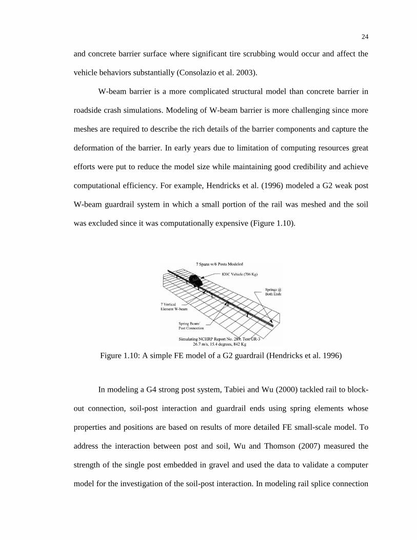
computational efficiency. For example, Hendricks et al. (1996) modeled a G2 weak post
W-beam guardrail system in which a small portion of the rail was meshed and the soil
was excluded since it was computationally expensive (Figure 1.10).
Figure 1.10: A simple FE model of a G2 guardrail (Hendricks et al. 1996)
In modeling a G4 strong post system, Tabiei and Wu (2000) tackled rail to block-
out connection, soil-post interaction and guardrail ends using spring elements whose
properties and positions are based on results of more detailed FE small-scale model. To
address the interaction between post and soil, Wu and Thomson (2007) measured the
strength of the single post embedded in gravel and used the data to validate a computer
model for the investigation of the soil-post interaction. In modeling rail splice connection
25
and its failure, Ray et al. (2001) found out that the major failure procedure of splice
connection was that rail got stretched, deformed into plastic region and the bolt then
slides through the hole or a rupture occurs. Since the bolt almost never failed, it may be
represented by computational efficient rigid material model.
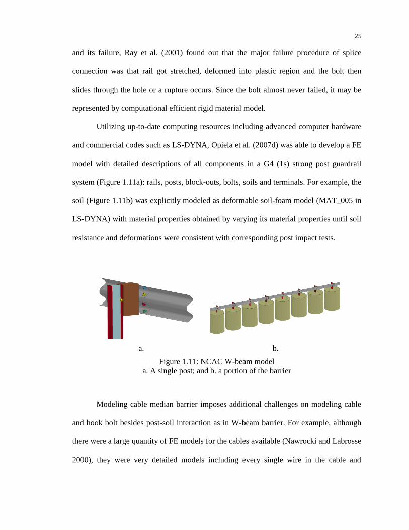
Utilizing up-to-date computing resources including advanced computer hardware
and commercial codes such as LS-DYNA, Opiela et al. (2007d) was able to develop a FE
model with detailed descriptions of all components in a G4 (1s) strong post guardrail
system (Figure 1.11a): rails, posts, block-outs, bolts, soils and terminals. For example, the
soil (Figure 1.11b) was explicitly modeled as deformable soil-foam model (MAT_005 in
LS-DYNA) with material properties obtained by varying its material properties until soil
resistance and deformations were consistent with corresponding post impact tests.
a. b.
Figure 1.11: NCAC W-beam model
a. A single post; and b. a portion of the barrier
Modeling cable median barrier imposes additional challenges on modeling cable
and hook bolt besides post-soil interaction as in W-beam barrier. For example, although
there were a large quantity of FE models for the cables available (Nawrocki and Labrosse
2000), they were very detailed models including every single wire in the cable and
26
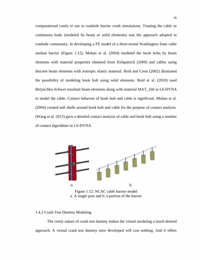
computational costly to use in roadside barrier crash simulations. Treating the cable as
continuous body (modeled by beam or solid elements) was the approach adopted in
roadside community. In developing a FE model of a three-strand Washington State cable
median barrier (Figure 1.12), Mohan et al. (2004) modeled the hook bolts by beam
elements with material properties obtained from Kirkpatrick (2000) and cables using
discrete beam elements with isotropic elastic material. Reid and Coon (2002) illustrated
the possibility of modeling hook bolt using solid elements. Reid et al. (2010) used
Belytschko-Schwer resultant beam elements along with material MAT_166 in LS-DYNA
to model the cable. Contact behavior of hook bolt and cable is significant. Mohan et al.
(2004) created null shells around hook bolt and cable for the purpose of contact analysis.
(Wang et al. 2013) gave a detailed contact analysis of cable and hook bolt using a number
of contact algorithms in LS-DYNA.
a. b.
Figure 1.12: NCAC cable barrier model
a. A single post and b. a portion of the barrier
1.4.3 Crash Test Dummy Modeling
The costly nature of crash test dummy makes the virtual modeling a much desired
approach. A virtual crash test dummy once developed will cost nothing. And it offers
27
additional instrumentation capabilities which are hard or impossible to implement in a
physical crash test dummy. The virtual computer dummy model provides better
repeatability, predictability and more channels to obtain information about what is
happening to the dummy during a crash. On the contrary, real world crash test dummy
hardware is limited by their instrumentation capabilities.
Most of the dummy modeling is aimed for the real world crash test dummies, not
the real human beings and this strategy is referred as “crash test dummy based modeling”.
The reasons behind this are: (1) crash test dummies enjoy the most test data which can be
used to validate the developed dummy models; (2) experiments with the crash test
dummies are usually available; if not they can be relatively easy to be designed and
carried out. This is difficult if not impossible for direct experiments involving with
human bodies.
In developing FE models of crash test dummies, the whole dummy is
disassembled into a number of units such as head, neck, shoulders, thorax, lumbar spine,
pelvis, lower extremities, and upper extremities. Each of these units is composed of a few
small components. FE modeling of crash test dummies usually starts with geometric
model building of the smallest components and their components material testing. These
individual components with reasonable meshes and material properties are assembled
into their corresponding larger unit. At the unit level various testing was done to ensure
consistent results between FE simulations and tests (Arnoux et al. 2003). For example,
the head undergoes free drop test and the neck and the thorax go through a pendulum test.
The units will be assembled into the complete dummy with appropriate joint and different
28
constraints connections. Finally the entire FE model of dummy is validated in a sled
testing configuration.
The balance between accuracy and efficiency depends on the nature of the study
performed and available computing resources. With significant simplifications dummy
modeling in the early 1990s saw Schelkle and Remensperger (1991a) developed the first
Hybrid III FE model developed which had only about 5,000 nodes and 3,000 elements.
Khalil and Lin (1991) did a comprehensive modeling of the Hybrid III dummy thorax for
DYNA3D and Khalil and Lin (1994) included every Hybrid III dummy unit such as head,
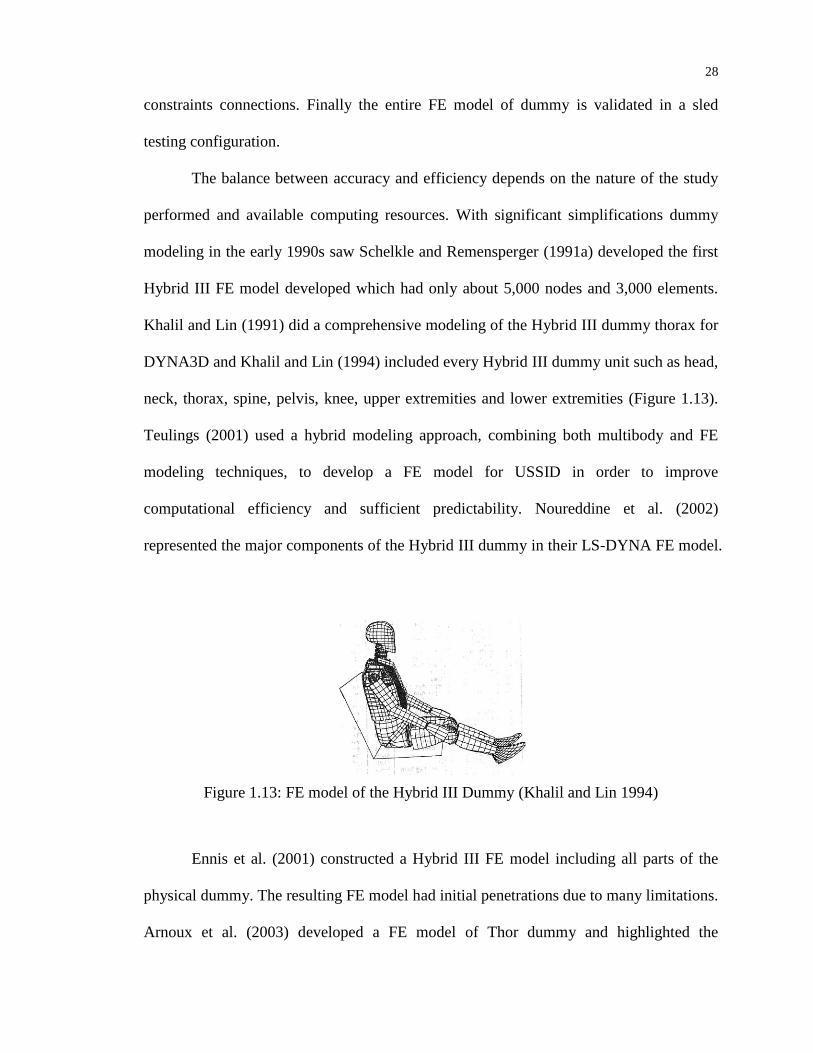
neck, thorax, spine, pelvis, knee, upper extremities and lower extremities (Figure 1.13).
Teulings (2001) used a hybrid modeling approach, combining both multibody and FE
modeling techniques, to develop a FE model for USSID in order to improve
computational efficiency and sufficient predictability. Noureddine et al. (2002)
represented the major components of the Hybrid III dummy in their LS-DYNA FE model.
Figure 1.13: FE model of the Hybrid III Dummy (Khalil and Lin 1994)
Ennis et al. (2001) constructed a Hybrid III FE model including all parts of the
physical dummy. The resulting FE model had initial penetrations due to many limitations.
Arnoux et al. (2003) developed a FE model of Thor dummy and highlighted the

29
difficulties of selecting appropriate material models especially energy dissipation soft
materials, damping systems and joints. Mohan et al. (2007), Mohan et al. (2009b) and
Mohan et al. (2010) presented modeling efforts of the Hybrid III 50th
male dummy for
LS-DYNA.
Besides Hybrid III dummy, the most popular FID, a number of FE models of
SIDs have also been developed. For example, in 1999, the German Association for
Automotive Research released USSID FE model (Franz et al. 1999) and Franz et al.
(2003) developed FE models for EuroSID. Gehre et al. (2009) and Gromer et al. (2009)
presented preliminary results of WorldSID 50th
percentile FE model.
Many virtual models of crash test dummies have been developed over the past
two decades, and extensive validation studies have been conducted with satisfying results.
These models are directly based on mechanical hardware. There is one significant
disadvantage with this approach: a long period of time delay before new findings can be
implemented in crash dummy hardware. For instance, the Hybrid III crash test dummy,
the most used dummy, is based mainly on biomechanical knowledge that is more than
twenty years old. New scientific findings have not resulted in much improvements in its
design since safety regulations from government and agencies, which specify the Hybrid
III dummy as a regulatory test device, is slow to accept new specifications in the
regulation. As a result, the Hybrid III dummy used today is much the same ever since it
was developed in the 1970s. This delay in scientific knowledge transfer is less severe in a
design strategy based directly on human body. It is more likely to rapidly benefit from
new scientific knowledge of injury mechanisms and injury criteria obtained through
biomechanical research since there is no need to construct its hardware. What is more,
30
these models will resemble a real human body in geometry and structures and naturally
allow the study of the effect of body size, posture influence as well as muscular activity.
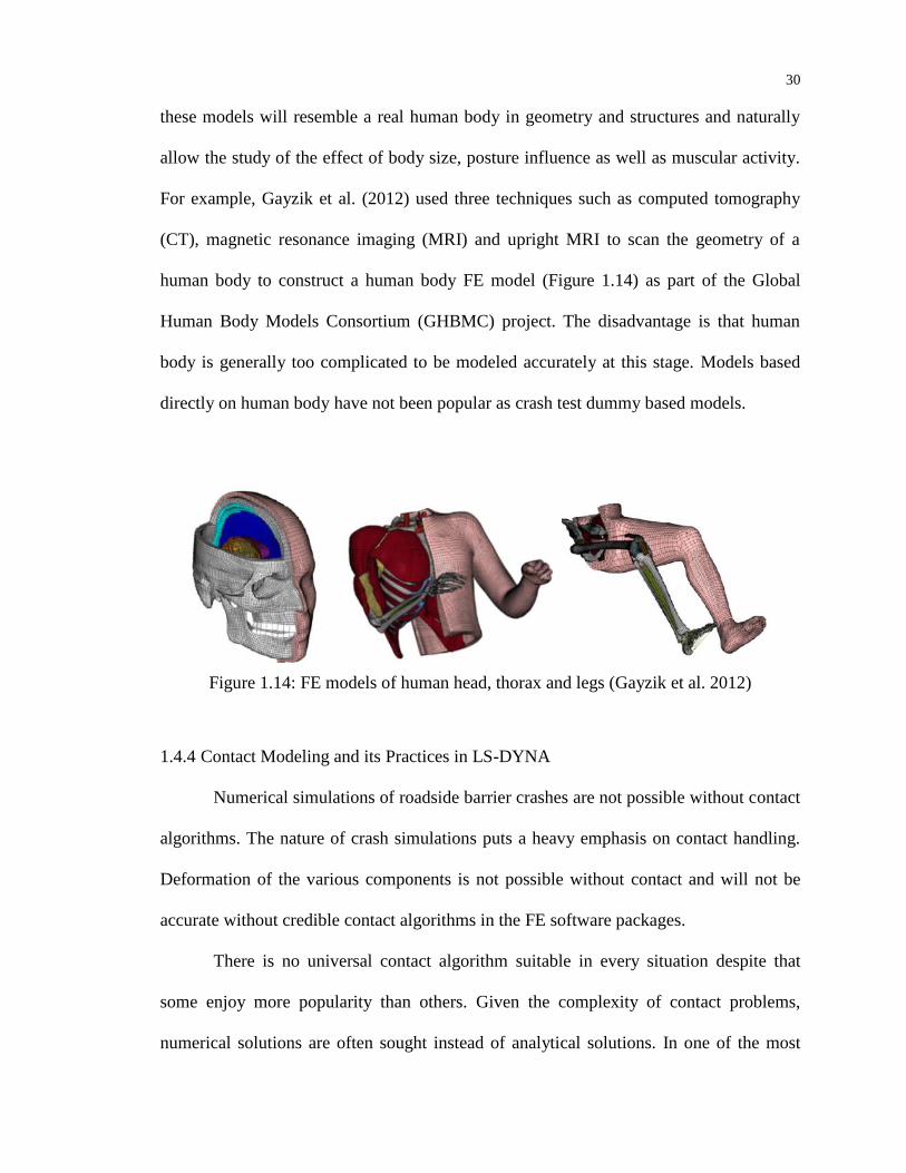
For example, Gayzik et al. (2012) used three techniques such as computed tomography
(CT), magnetic resonance imaging (MRI) and upright MRI to scan the geometry of a
human body to construct a human body FE model (Figure 1.14) as part of the Global
Human Body Models Consortium (GHBMC) project. The disadvantage is that human
body is generally too complicated to be modeled accurately at this stage. Models based
directly on human body have not been popular as crash test dummy based models.
Figure 1.14: FE models of human head, thorax and legs (Gayzik et al. 2012)
1.4.4 Contact Modeling and its Practices in LS-DYNA
Numerical simulations of roadside barrier crashes are not possible without contact
algorithms. The nature of crash simulations puts a heavy emphasis on contact handling.
Deformation of the various components is not possible without contact and will not be
accurate without credible contact algorithms in the FE software packages.
There is no universal contact algorithm suitable in every situation despite that
some enjoy more popularity than others. Given the complexity of contact problems,
numerical solutions are often sought instead of analytical solutions. In one of the most
31
used numerical techniques, FE analysis, contact algorithms are often distinguished based
on the discretization technique used for the contacting interfaces such as node-to-segment
(NTS), mortar segment-to-segment, etc. The NTS algorithm is probably the most widely
used discretization technique for large deformation contact between surfaces with non-
matching meshes partially due to its simplicity, especially in commercial FE code
packages (Hallquist et al. 1985).
NTS imposes the contact constraints point-wisely at a finite number of slave
nodes, i.e. only the nodal points are checked and not allowed to penetrate into the master
segment. NTS lacks numerical robustness as a result of contact constraints imposed only
on a finite number of the slave nodal points (Puso and Laursen 2004a); its poor
convergence properties are particularly evident when implicit solution procedures are
used.
The development of so called mortar formulations, or mortar segment-to-segment
(Laursen et al. 2012) is aimed to improve convergence for contact problems. Contact
constraints are enforced along the entire contact boundary, instead of constraining only
the slave nodal points. This produces a stronger confinement between the degrees of
freedom of the contacting interfaces and a smoother contact pressure distribution.
Both NTS and mortar approach deal with c0 continuous contacting surface
(faceted surface) which deteriorates the convergence rate. Higher-order geometrical
descriptions shall improve smoothness in contact pressure and solve the problem of non-
physical oscillations of contact forces induced by the traditional enforcement of
kinematic contact constraints via faceted surfaces in traditional FE. The concept of
isogeometric analysis introduced by Hughes et al. (2005), using NURBS to represent the

32
geometry of contacting bodies and their surfaces exactly without any approximations, is
promising in improve convergence in contact problems. Using the spirit of isogeometric
analysis, Temizer et al. (2011) developed a knot-to-surface (KTS) contact algorithm for
frictionless contact surface discretized by NURBS and Temizer et al. (2012) extended
isogeometric contact analysis to the mortar based KTS Algorithm for frictional contact
problems.
As one of the most successful explicit code used in roadside barrier crashes
community, development of contact algorithms in LS-DYNA has gone through several
decades and numerous contact keywords have been developed to handle contact
problems with various complexities (Table 1.2). It is one of the main commercial FE
codes used in crash analysis especially automobile crash simulations.

33
Table 1.2: A list of commonly used contact algorithms in LS-DYNA
Contact Type ID Keyword (prefix with“*CONTACT_”)
1 SLIDING_ONLY
2 TIED_SURFACE_TO_SURFACE
3 SURFACE_TO_SURFACE
4 SINGLE_SURFACE
5 NODES_TO_SURFACE
6 TIED_NODES_TO_SURFACE
7 TIED_SHELL_EDGE_TO_SURFACE
10 ONE_WAY_SURFACE_TO_SURFACE
13 AUTOMATIC_SINGLE_SURFACE
17 CONSTRAINT_SURFACE_TO_SURFACE
18 CONSTRAINT_NODES_TO_SURFACE
22 SINGLE_EDGE
26 AUTOMATIC_GENERAL
a3 AUTOMATIC_SURFACE_TO_SURFACE
a5 AUTOMATIC_NODES_TO_SURFACE
a13 AIRBAG_SINGLE_SURFACE
i26 AUTOMATIC_GENERAL_INTERIOR
As the predominant contact algorithm used in crash analysis, penalty method
enjoys many contact keywords and hundreds of parameters which could be tuned to
achieve optimal contact behavior. Picking up the most appropriate contact keyword in
LS-DYNA is no easy task and requires intensive experience. Penalty method needs a user
controlled penalty stiffness which is the most critical single parameter affecting contact
treatment accuracy. Three different algorithms of determining the penalty parameter are
available in LS-DYNA: standard penalty formulation (SOFT1=0), soft constraint penalty
formulation (SOFT=1) and segment based penalty formulation (SOFT=2) (Hallquist
2006). In standard formulation, the interface stiffness2 is chosen to be based on
material elastic constants and element dimensions, approximately the same order of
magnitude as the stiffness of the interface element normal to the interface. Consequently
1 SOFT is an input parameter defined in a contact keyword card in LS-DYNA.
2 Interface stiffness, or penalty stiffness, or penalty parameter is used interchangeably.
34
the computed time-step size is unaffected by the existence of the interface; if the interface
pressure becomes large unacceptable penetration may occur. In the soft constraint method,
the penalty stiffness takes into the global time-step and contacting nodal masses
accounts. seeks to increasing contact stiffness while maintaining stable contact
behavior. In foam and plastic materials, the contact stiffness and can differ
by one or more orders of magnitude. In segment based penalty formulation, the penalty
stiffness calculates contact stiffness much like the soft constraint method except
that the square of time-step is used in the calculation of contact stiffness. Segment-based
contact can often be quite effective where other methods fail at treating contact at sharp
corners of parts.
Majority of contact definitions in LS-DYNA place a limit on the maximum
penetration depth, i.e. contact threshold, and the slave node is released free from contact
constraint and its corresponding contact forces are set to zero. For example, in one of the
most used contact keyword *CONTACT_AUTOMATIC_SINGLE_SURFACE (Type 13
contact), the contact threshold is defined as one half of the thickness of the solid elements
or 40% of the sum of slave thickness and master thickness for shell elements. By
releasing the nodes large contact forces will be avoided and the contact behavior should
be more stabilized. An important consequence is that extremely thin shell elements
defined in the contact is likely to fail the contact handling in case that the maximum
penetration depth has been reached early in the simulation. For example, the airbag fabric
shell is often very thin and artificial enlargement of the shell thickness will help combat
contacting instabilities.
35
In practice a so called “single contact approach” defining only one contact card
such as CONTACT_AUTOMATIC_SINGLE_SURFACE that includes all parts which
may potentially come into contact is preferred from the standpoints of simplicity in
preprocessing, numerical robustness, and computational efficiency.
In Chapter 2, a detailed review of contact analysis with the emphasis on numerical
implementations is conducted. In Chapter 3, a FE model of a 2006 Ford F250 will be
presented and validated in frontal impacts. Chapter 4 will provide insights of the
modeling efforts of a Hybrid III 50th
percentile male dummy. Chapter 5 will discuss the
roadside barrier crash simulations using established FE models of vehicle, dummy and
barrier. Chapter 6 will be devoted to the analysis of the occupant injuries. Finally,
Chapter 7 will conclude the dissertation.
CHAPTER 2: CONTACT ANALYSIS
Contact analysis is central to crash problems, because they involve a large number
of deformable bodies being in contact. Although contacts are often simplified and
substituted in many non-crash related problems, the presence of contacts is critical in the
case of roadside barrier crashes because it determines the accuracy of the vehicular
responses and the barrier performances.
Due to the complexity of contact problems, numerical solutions are often sought
for most engineering problems rather than analytical solutions. Over the years, numerical
algorithms of different contact methods have been implemented into the FE codes, which
have been applied to solve many of contact problems with good accuracy.
In this chapter, a brief discussion of numerical implementations of contact
theories shall be given in section 2.1 and some details of the contact algorithms in LS-
DYNA in section 2.2.
2.1 Numerical Implementations of Contact Theories
Since the work of Heinrich Hertz on solving a frictionless contact problem of two
ellipsoidal elastic bodies, known as the “Hertz contact” (Figure 2.1), contact mechanics
has been considerably advanced in seeking theoretical and especially numerical solutions
of particular contact problems in engineering systems.
37
Figure 2.1: Contact of two spheres with linear elastic properties and small deformation
It is fair to say that solving contact problems is among the most difficult ones in
mechanics. Contact unilateral inequalities, i.e. the physical impossibility of tensile
contact traction (except some special problems, e.g. structures are glued together) and of
material interpenetration, combined with nonlinearities introduced by friction laws and
material models, can greatly complicate the problems. The complexity and popularity of
contact problems was well illustrated by Zhong and Mackerle (1992) who gave a
bibliography including seven hundred papers solely related to static contact problems and
published in journals and conference proceedings from 1976 to 1992. Due to the
difficulties in solving contact problems analytically, seeking numerical solutions have
largely surpassed the analytical approach in explaining most contact problems especially
in engineering applications. In particular, the FE method has been widely used to solve
contact problems with various grades of complexity. Despite of numerous researches
over many years contact problem is still a very challenging topic (Puso and Laursen
2004a) even in the framework of numerical solutions. For example, Franke et al. (2010)
who investigated on the classical 2D Hertz contact problem and found “significantly
varying results for different finite element versions” (h-, p-, hp-, and rp-version) using the

38
most popular penalty method with adjusted penalty parameter and refined meshes
covering the contact region.
Numerical implementation of contact methods into FE codes start with
mathematical formulation of the contact constraints. Of all the contact formulations, the
Lagrangian multiplier method, the penalty method, and the perturbed Lagrange
formulation are among the most common ways to enforce contact constraints. These
methods can be understood by examine potential energy of a mechanical system. Assume
the potential energy for a dynamic system as without considering contact constraints,
it takes the simple form as
T T T T
p pd d d d
u a u b u t U F (2.1)
where is the strain tensor, is the strain tensor, u is the displacement, a is the
acceleration, is the material density, b is the body force, is the body region, is the
surface area where traction t applies and pU is the displacement at point on which
concentrated load pF act.
The Lagrangian multiplier method handles the contact constraints by adding
energy term to
T d
C u (2.2)
where is the unknown Lagrangian multiplier and
0C u
(2.3)
is the contact constraint function.
The penalty method will enforce the contact constraint by adding energy term to
39
T d
C u C u (2.4)
where is the user controlled penalty parameter.
The perturbed Lagrange formulation combines the Lagrangian multiplier term in
(2.2) and the penalty parameter term in (2.4),
T Td d
C u C u C u (2.5)
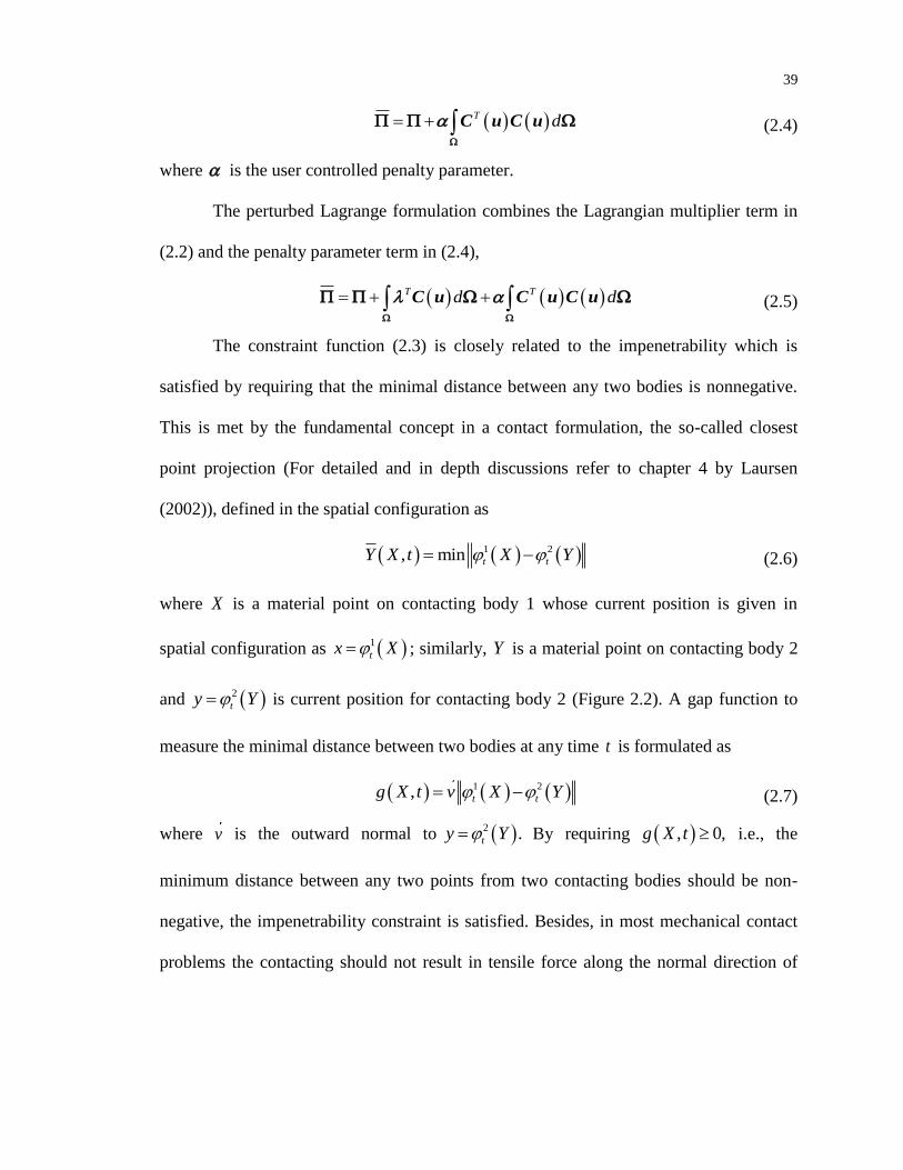
The constraint function (2.3) is closely related to the impenetrability which is
satisfied by requiring that the minimal distance between any two bodies is nonnegative.
This is met by the fundamental concept in a contact formulation, the so-called closest
point projection (For detailed and in depth discussions refer to chapter 4 by Laursen
(2002)), defined in the spatial configuration as
1 2, min t tY X t X Y (2.6)
where X is a material point on contacting body 1 whose current position is given in
spatial configuration as 1
tx X ; similarly, Y is a material point on contacting body 2
and 2
ty Y is current position for contacting body 2 (Figure 2.2). A gap function to
measure the minimal distance between two bodies at any time t is formulated as
1 2, t tg X t v X Y (2.7)
where v is the outward normal to 2 .ty Y By requiring , 0,g X t i.e., the
minimum distance between any two points from two contacting bodies should be non-
negative, the impenetrability constraint is satisfied. Besides, in most mechanical contact
problems the contacting should not result in tensile force along the normal direction of
40
the contacting interface. Mathematically this is equivalent to , 0t t v where is the
traction on the contacting interface.
Figure 2.2: Distance between surfaces of body 1 and body 2
Numerical implementation of contact methods into FE codes is complicated even
without considering the frictional effect and material nonlinearity. The Lagrangian
multiplier method, penalty method, and perturbed Lagrangian method are the popular
contact formulations implemented by a number of researchers. For example, Hughes et al.
(1976) used the Lagrangian multiplier method in an implicit FE code for a class of Hertz
static contact problems that assumed “the contact surface is approximately planar and the
bodies have undergone small straining in the neighborhood if the contact surface.” The
most significant contribution of the work lied in the discretized impact and release
conditions that were consistent with the wave propagation theory. The Lagragian
multipliers were the unknown contact forces at the individual contact nodes and once
negative contact force was found its corresponding contacting node was released from the
contact constraint.
41
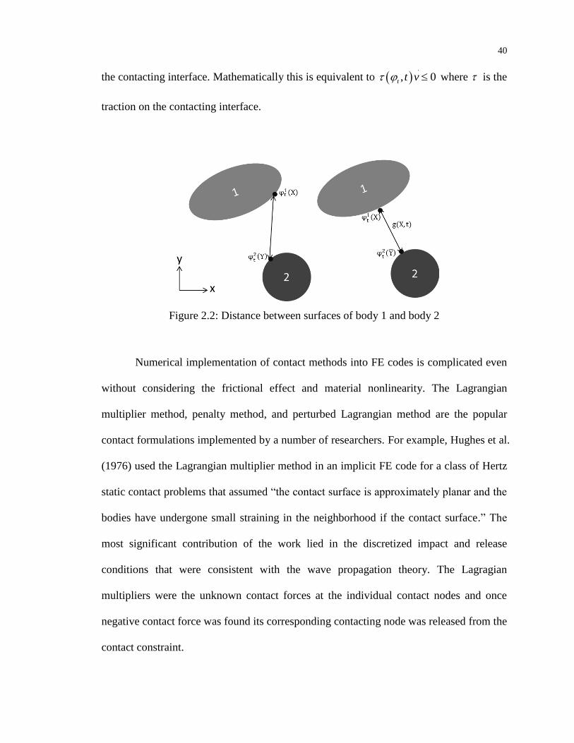
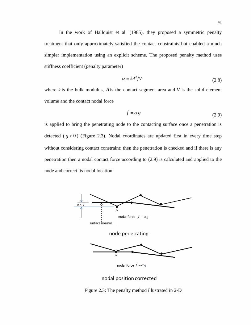
In the work of Hallquist et al. (1985), they proposed a symmetric penalty
treatment that only approximately satisfied the contact constraints but enabled a much
simpler implementation using an explicit scheme. The proposed penalty method uses
stiffness coefficient (penalty parameter)
2kA V (2.8)
where k is the bulk modulus, A is the contact segment area and V is the solid element
volume and the contact nodal force
f g (2.9)
is applied to bring the penetrating node to the contacting surface once a penetration is
detected ( 0g ) (Figure 2.3). Nodal coordinates are updated first in every time step
without considering contact constraint; then the penetration is checked and if there is any
penetration then a nodal contact force according to (2.9) is calculated and applied to the
node and correct its nodal location.
Figure 2.3: The penalty method illustrated in 2-D
42
Neither the Lagrangian multiplier method nor the penalty method is perfect or
ideal. Each method targets a certain class of contact problems and has its own advantages
and disadvantages. In general, the Lagrangian multiplier method is computationally
inefficient due to the large number of introduced unknowns (the Lagrangian multipliers)
in the equations and the associated cost of solving the equations. The penalty method is
computationally efficient due to the use of an explicit algorithm and without introducing
extra unknowns. However, its accuracy depends on the choice of the penalty parameter,
which determines the level of contact constraint satisfaction. Since the contact constraint
can only be fully satisfied with an infinite penalty parameter, this method suffers solution
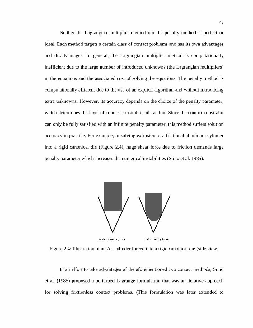
accuracy in practice. For example, in solving extrusion of a frictional aluminum cylinder
into a rigid canonical die (Figure 2.4), huge shear force due to friction demands large
penalty parameter which increases the numerical instabilities (Simo et al. 1985).
Figure 2.4: Illustration of an Al. cylinder forced into a rigid canonical die (side view)
In an effort to take advantages of the aforementioned two contact methods, Simo
et al. (1985) proposed a perturbed Lagrange formulation that was an iterative approach
for solving frictionless contact problems. (This formulation was later extended to

43
frictional contact problems by Simo and Laursen (1992). For large deformation, see
(Pietrzak and Curnier 1999)). Unlike the Lagrangian multiplier method where the
unknown multipliers are solved along with the displacements, the perturbed Lagrange
formulation used augmentation mechanism
1k k
kg (2.10)
to update the Lagrangian multiplier from iteration k to 1k until the gap function kg
at iteration k is reduced to a predefined tolerance value 0g and avoid solving the
Lagrangian multipliers. The proposed treatment comparing to the penalty method
converges to exact satisfaction of constraints with finite penalties. Numerically
satisfaction of the constraints can be improved even if penalty parameter is undersized
through an iterative procedure; this is extremely useful when large penalty parameter is
required (Figure 2.4). A number of augmentation mechanism has since been proposed
(Zavarise and Wriggers 1999) to facilitate the converging process; for example, Wriggers
and Zavarise (2008) modified the algorithm by replacing the Lagrangian term with
CAUCHY’S stress in the contacting interface.
Similar to the patch test used in FE analysis, patch tests were also designed to
examine the performance of a contact algorithm for contact problems. Specifically the
patch test checks whether a contact formulation is capable of exactly transmitting
constant normal stresses between two contacting surfaces, regardless of their
discretization schemes. Taylor and Papadopoulos (1991) first introduced a patch test for
contact problems to assess the accuracy of contact algorithms. A simple FE completeness
check - two bodies being compressed to each other under a uniform pressure (see Figure
2.5) - for frictionless contact in two dimensions was proposed where the classical
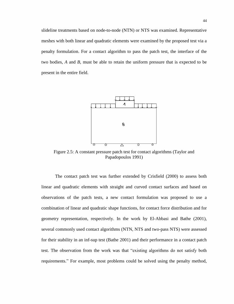
44
slideline treatments based on node-to-node (NTN) or NTS was examined. Representative
meshes with both linear and quadratic elements were examined by the proposed test via a
penalty formulation. For a contact algorithm to pass the patch test, the interface of the
two bodies, A and B, must be able to retain the uniform pressure that is expected to be
present in the entire field.
Figure 2.5: A constant pressure patch test for contact algorithms (Taylor and
Papadopoulos 1991)
The contact patch test was further extended by Crisfield (2000) to assess both
linear and quadratic elements with straight and curved contact surfaces and based on
observations of the patch tests, a new contact formulation was proposed to use a
combination of linear and quadratic shape functions, for contact force distribution and for
geometry representation, respectively. In the work by El-Abbasi and Bathe (2001),
several commonly used contact algorithms (NTN, NTS and two-pass NTS) were assessed
for their stability in an inf-sup test (Bathe 2001) and their performance in a contact patch
test. The observation from the work was that “existing algorithms do not satisfy both
requirements.” For example, most problems could be solved using the penalty method,
45
but the solutions had significant numerical errors and were not guaranteed to have
numerical stability.
The differences among the Lagrangian multiplier method, penalty method, and
perturbed Lagrangian method lie in how constraints are handled in the contact
formulation. In the numerical implementations of contact formulations into the FE codes,
contact algorithms are more often distinguished based on the FE mesh or discretization
techniques from which the contact interfaces are defined such as NTS, mortar segment-
to-segment, etc. NTS can be used with either penalty method in an explicit scheme
(Hallquist et al. 1985) or with the Lagrangian multiplier method in an implicit scheme
(Hughes et al. 1976). NTS can also be used with the Lagrangian multiplier method in an
explicit scheme (Zhong 1993).
2.1.1 Node-to-segment Contact Algorithms
The NTS contact algorithm is commonly used for handling large deformation
contacts between surfaces with non-matching meshes, especially in commercial FE codes,
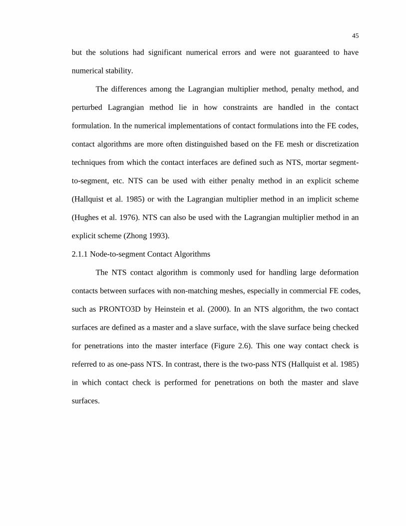
such as PRONTO3D by Heinstein et al. (2000). In an NTS algorithm, the two contact
surfaces are defined as a master and a slave surface, with the slave surface being checked
for penetrations into the master interface (Figure 2.6). This one way contact check is
referred to as one-pass NTS. In contrast, there is the two-pass NTS (Hallquist et al. 1985)
in which contact check is performed for penetrations on both the master and slave
surfaces.
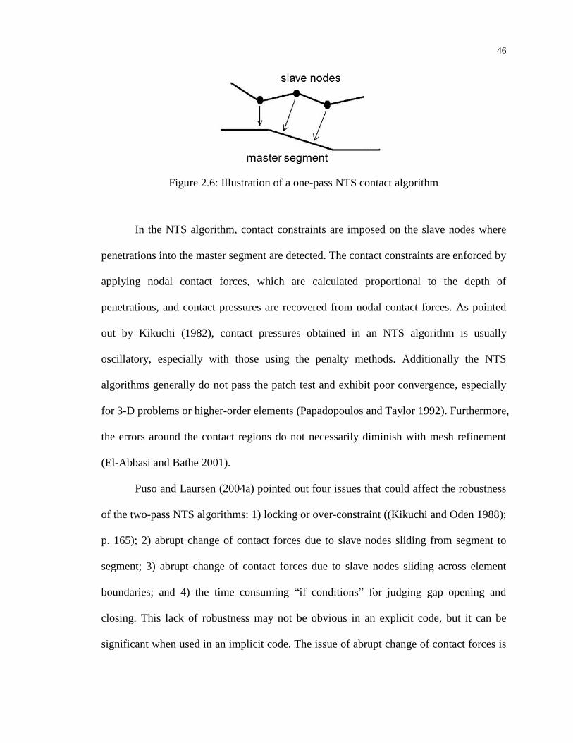
46
Figure 2.6: Illustration of a one-pass NTS contact algorithm
In the NTS algorithm, contact constraints are imposed on the slave nodes where
penetrations into the master segment are detected. The contact constraints are enforced by
applying nodal contact forces, which are calculated proportional to the depth of
penetrations, and contact pressures are recovered from nodal contact forces. As pointed
out by Kikuchi (1982), contact pressures obtained in an NTS algorithm is usually
oscillatory, especially with those using the penalty methods. Additionally the NTS
algorithms generally do not pass the patch test and exhibit poor convergence, especially
for 3-D problems or higher-order elements (Papadopoulos and Taylor 1992). Furthermore,
the errors around the contact regions do not necessarily diminish with mesh refinement
(El-Abbasi and Bathe 2001).
Puso and Laursen (2004a) pointed out four issues that could affect the robustness
of the two-pass NTS algorithms: 1) locking or over-constraint ((Kikuchi and Oden 1988);
p. 165); 2) abrupt change of contact forces due to slave nodes sliding from segment to
segment; 3) abrupt change of contact forces due to slave nodes sliding across element
boundaries; and 4) the time consuming “if conditions” for judging gap opening and
closing. This lack of robustness may not be obvious in an explicit code, but it can be
significant when used in an implicit code. The issue of abrupt change of contact forces is
47
related to the non-smooth FE meshes and makes it difficult for an implicit analysis to
converge. A new technique, called isogeometric analysis, is promising to overcome this
difficulty and may be considered for implementation into the FE codes.
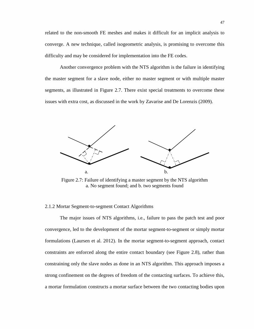
Another convergence problem with the NTS algorithm is the failure in identifying
the master segment for a slave node, either no master segment or with multiple master
segments, as illustrated in Figure 2.7. There exist special treatments to overcome these
issues with extra cost, as discussed in the work by Zavarise and De Lorenzis (2009).
a. b.
Figure 2.7: Failure of identifying a master segment by the NTS algorithm
a. No segment found; and b. two segments found
2.1.2 Mortar Segment-to-segment Contact Algorithms
The major issues of NTS algorithms, i.e., failure to pass the patch test and poor
convergence, led to the development of the mortar segment-to-segment or simply mortar
formulations (Laursen et al. 2012). In the mortar segment-to-segment approach, contact
constraints are enforced along the entire contact boundary (see Figure 2.8), rather than
constraining only the slave nodes as done in an NTS algorithm. This approach imposes a
strong confinement on the degrees of freedom of the contacting surfaces. To achieve this,
a mortar formulation constructs a mortar surface between the two contacting bodies upon

48
which the contact constraints are imposed (McDevitt and Laursen 2000). This
intermediate mortar surface was discretized by the so-called mortar elements, which
provide linear transformation of the displacement field for each contacting surface to the
intermediate mortar surface. On the mortar surface, contact constraints are enforced and
traction forces are calculated.
Figure 2.8: Illustration of a mortar contact: penetration is prevented over a region
The concept of contact segment dates back to the work of Simo et al. (1985) in
which the perturbed Lagrangian method was developed. Zavarise and Wriggers (1998)
were the first to explicitly use the name of segment-to-segment contact. The mortar
segment-to-segment has good convergence as demonstrated in a kinematically linear
context for contacting bodies with non-conformingly meshed (Hild 2000). Various
implementations of the mortar segment-to-segment contact algorithm were proposed,
such as the formulations using linear elements for 2D problems (Yang et al. 2005), using
bilinear elements for 3D problems (Puso and Laursen 2004a; b), and using quadratic
elements for 3d problems (Puso et al. 2008).
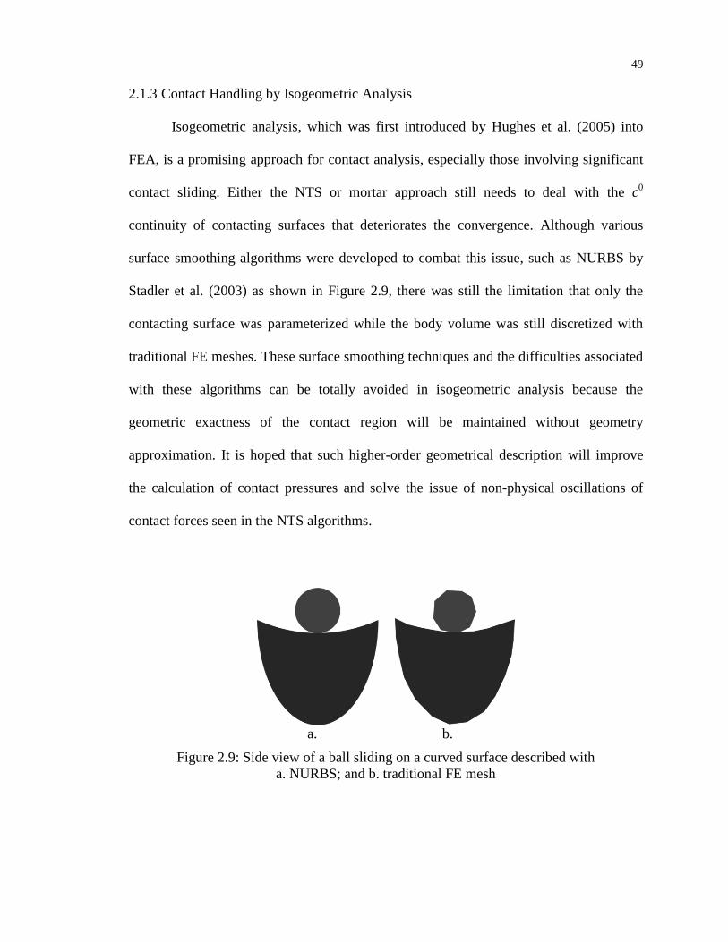
49
2.1.3 Contact Handling by Isogeometric Analysis
Isogeometric analysis, which was first introduced by Hughes et al. (2005) into
FEA, is a promising approach for contact analysis, especially those involving significant
contact sliding. Either the NTS or mortar approach still needs to deal with the c0
continuity of contacting surfaces that deteriorates the convergence. Although various
surface smoothing algorithms were developed to combat this issue, such as NURBS by
Stadler et al. (2003) as shown in Figure 2.9, there was still the limitation that only the
contacting surface was parameterized while the body volume was still discretized with
traditional FE meshes. These surface smoothing techniques and the difficulties associated
with these algorithms can be totally avoided in isogeometric analysis because the
geometric exactness of the contact region will be maintained without geometry
approximation. It is hoped that such higher-order geometrical description will improve
the calculation of contact pressures and solve the issue of non-physical oscillations of
contact forces seen in the NTS algorithms.
a. b.
Figure 2.9: Side view of a ball sliding on a curved surface described with
a. NURBS; and b. traditional FE mesh

50
Developing contact algorithms based on isogeometric analysis is still an ongoing
research. Lu (2011) introduced an isogeometric framework for contact analysis and
discussed NURBS parameterization, contact detection on patch level, smoothing sharp
corners, and a segment-to-segment formulation for frictionless contacts. Temizer et al.
(2011) developed a knot-to-surface (KTS) contact algorithm for frictionless contact
surfaces discretized by NURBS. In a KTS algorithm, contact constraints are enforced on
quadrature points. Quantitative studies based on the Hertz problem showed that the KTS
algorithm offered potential accuracy as well as convergence improvements over c0
continuous finite elements. De Lorenzis et al. (2011) proposed a mortar-based NURBS
isogeometric analysis to treat the Coulomb frictional contact constraints. Temizer et al.
(2012) further extended isogeometric contact analysis to the mortar based KTS algorithm
for frictional contact problems. Recently, Kim and Youn (2012) proposed a new contact
matching and detection algorithm for identifying contacting regions of NURBS-
represented geometries based on the mortar method.
2.2 Contact Modeling in LS-DYNA
The development of contact algorithms in LS-DYNA has been ongoing since
Livermore Software Technology Corporation (LSTC) was founded in 1987 by John O.
Hallquist to commercialize DYNA3D developed at the Lawrence Livermore National
Laboratory. Prior to 1987, traditional hydrocodes using explicit finite difference method
such as HEMP (Wilkins 1963) and TENSOR (Maenchen and Sack 1963) had been
successfully used to deal with extremely large contact pressures. The strategy is often
referred as hydrocode approach or slideline treatment. In LS-DYNA, the simple and
inexpensive penalty method was implemented (Benson and Hallquist 1990; Hallquist et
51
al. 1985) for both explicit and implicit integration algorithms rather than the Lagrangian
multiplier method (Chaudhary and Bathe 1985; Hughes et al. 1976). Many LS-DYNA
implementations of contact algorithms share the same basic methods as described by
Benson and Hallquist (1990) and Hallquist et al. (1985) but differ in means of
enrichments and improvements.
2.2.1 Contact Algorithms used in LS-DYNA
The current version of LS-DYNA provides three methods for contact treatment:
kinematic constraint method, the penalty method, and the distributed parameter method.
All these methods are implemented into the explicit LS-DYNA codes. The development
of distributed parameter method was motivated by TENSOR (Burton et al. 1982) and
HEMP (Wilkins 1963) and it has remained unchanged since its early implementation in
DYNA2D (Hallquist 1978). This contact treatment is defined as a sliding only contact
(*CONTACT_SLIDING_ONLY) in LS-DYNA, i.e., the slave surface can slide on the
master surface but cannot be separated from it. This sliding only contact is mainly used in
high explosive environment and rarely used in the context of automobile crash
simulations.
The kinematic constraint method was motivated by the work of Hughes et al.
(1976) where impact and release conditions were enforced to conserve momentum. The
basic concept was that the slave parts was brought against the master part unless a tensile
stress was developed on the interface and if so the slave part would be released from the
contact constraint. In LS-DYNA, this concept was used to develop the tied contact or
tying contact. In the tying contact, the slave nodes/surfaces are always constrained to the
master surfaces. As the name implies, tied contacts are used to constrain two surfaces

52
together without relative motion and are generally not penalty based methods. The
rotational degrees of freedom are not constrained in tied contacts; thus it is recommended
that nodes used in TIED_NODES_TO_SURFACE and
TIED_SURFACE_TO_SURFACE contacts are not connected to any structural nodes
with rotational degrees of freedom (e.g., nodes of shell and beam elements). For example,
tying a part modeled with solid elements to a part modeled with shell/beam elements is
not a recommended practice.
In a tied contact in LS-DYNA, slave nodes are forced to stay close to the master
surface; this may results in distortion or modification of the slave surface geometry.
Therefore, it is important to ensure that the two surfaces in a tied contact are not too far
away from each other to avoid significant elements distortions. In tied contact, the slave
and master surfaces are distinguished because constraints are not applied symmetrically,
i.e. the slave surface always subdues to the master surface. When two parts of similar
materials are defined in a tied contact, the master surface is typically defined on the one
with coarser meshes. For parts of significantly different materials in a tied contact, the
master surface is typically chosen on the one with a stiffer material.
The penalty method, despite it is simple in concept, is implemented in LS-DYNA
with enriched contact handling and as the dominant contact algorithm for crash analysis.
Unlike the Lagrangian multiplier method and perturbed Lagrangian method, the penalty
method uses a user defined/controlled penalty stiffness that is the most critical single
parameter affecting contact treatment accuracy. Three different formulations of
calculating the penalty stiffness so as to provide contact stability and reasonable accuracy
are available in LS-DYNA: the standard penalty formulation (SOFT=0), the soft
53
constraint penalty formulation (SOFT=1), and the segment-based penalty formulation
(SOFT=2) (Hallquist 2006). In the standard formulation, the interface stiffness is chosen
with the same order of magnitude as the stiffness of the interface materials. Consequently
the computed time-step size is unaffected by the existence of the interface and
unacceptable penetration may occur if the interface pressure becomes large. When
SOFT=1, the penalty stiffness is proportional to the contacting nodal masses and the
inverse of time-step. The soft constraint stiffness method is recommended for contacts
among parts of dissimilar mesh sizes and/or dissimilar material properties. In this case,
all parts are defined in a global slave set for the Type 13 contact
(*AUTOMATIC_SINGLE_SURFACE) in which no master part is required; the soft
constraint method seeks to maximize contact stiffness while maintaining a stable contact
behavior. The primary disadvantage of choosing the soft constraint method is its
dependence on the global time-step. Occasionally, the global time-step must be scaled
down to avoid numerical instabilities in the contact behavior. This results in an increased
run time for the entire simulation. In the segment-based contact method, the contact
stiffness is calculated similar to that in the soft constraint method but differs in that it is
proportional to the inverse of square of time-step and the initial time-step is maintained
and only updated if the solution time-step is increased by more than 5%. Segment-based
contacts can be quite effective where other methods may fail, e.g., in the contact handling
involving sharp edges or corners.
2.2.2 Penetration Depth Calculation
In a penalty formulation, the penalty parameter and penetration distance are most
important quantities. The penalty parameter has a default value in LS-DYNA and it can
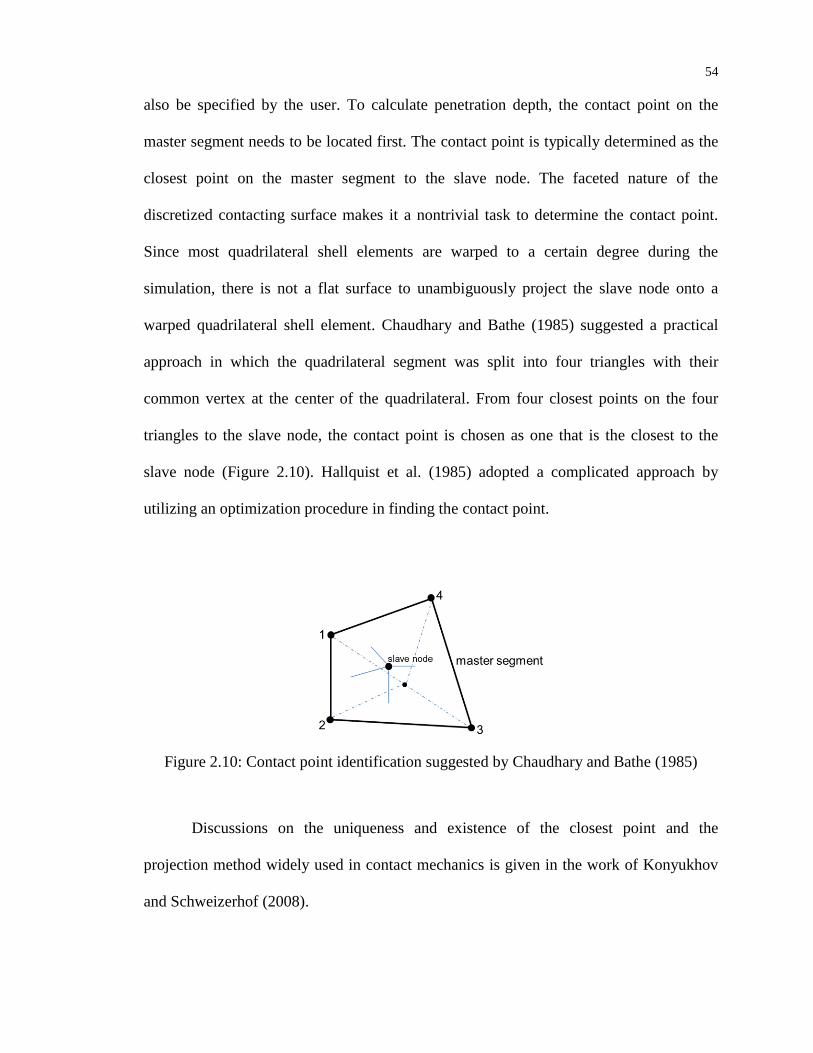
54
also be specified by the user. To calculate penetration depth, the contact point on the
master segment needs to be located first. The contact point is typically determined as the
closest point on the master segment to the slave node. The faceted nature of the
discretized contacting surface makes it a nontrivial task to determine the contact point.
Since most quadrilateral shell elements are warped to a certain degree during the
simulation, there is not a flat surface to unambiguously project the slave node onto a
warped quadrilateral shell element. Chaudhary and Bathe (1985) suggested a practical
approach in which the quadrilateral segment was split into four triangles with their
common vertex at the center of the quadrilateral. From four closest points on the four
triangles to the slave node, the contact point is chosen as one that is the closest to the
slave node (Figure 2.10). Hallquist et al. (1985) adopted a complicated approach by
utilizing an optimization procedure in finding the contact point.
Figure 2.10: Contact point identification suggested by Chaudhary and Bathe (1985)
Discussions on the uniqueness and existence of the closest point and the
projection method widely used in contact mechanics is given in the work of Konyukhov
and Schweizerhof (2008).

55
Since the normal direction at the contact point may not be uniquely defined, the
penetration depth thus calculated is often not unique. There are at least two ways to
determine a normal direction at the contact point: 1) based on the master surface normal
of the contact point; and 2) by the velocity direction of slave node (Figure 2.11). These
two choices should result in different directions and thus different penetration depth and
force direction. The wisdom of choosing the “correct” method is not immediately clear
but according to Hallquist et al. (1985), “in most problems, using the normal at the
contact point results in an acceptable solution, but in some situations, evaluating the
contact force with the slave normal results in a much better solution”.
a. b.
Figure 2.11: Determination of a normal direction of the contact point by
a. Surface normal of the master segment; and b. velocity direction of slave node
The majority contact definitions in LS-DYNA have a limit on the maximum
penetration depth beyond which the slave node is released from contact constraint and the
corresponding contact forces are set to zero. For example, in one of the commonly used
contacts, Type 13 contact, the maximum penetration depth is defined as one half of the
thickness for the solid elements or 40% of the total thickness of the slave and master
segments combined for shell elements. This node releasing mechanism helps avoid large
contact forces and stabilize the contact behavior. For extremely thin shell elements used
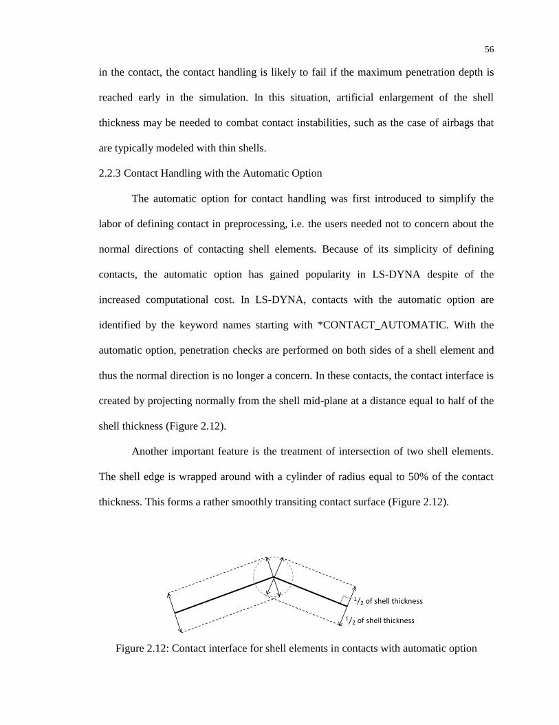
56
in the contact, the contact handling is likely to fail if the maximum penetration depth is
reached early in the simulation. In this situation, artificial enlargement of the shell
thickness may be needed to combat contact instabilities, such as the case of airbags that
are typically modeled with thin shells.
2.2.3 Contact Handling with the Automatic Option
The automatic option for contact handling was first introduced to simplify the
labor of defining contact in preprocessing, i.e. the users needed not to concern about the
normal directions of contacting shell elements. Because of its simplicity of defining
contacts, the automatic option has gained popularity in LS-DYNA despite of the
increased computational cost. In LS-DYNA, contacts with the automatic option are
identified by the keyword names starting with *CONTACT_AUTOMATIC. With the
automatic option, penetration checks are performed on both sides of a shell element and
thus the normal direction is no longer a concern. In these contacts, the contact interface is
created by projecting normally from the shell mid-plane at a distance equal to half of the
shell thickness (Figure 2.12).
Another important feature is the treatment of intersection of two shell elements.
The shell edge is wrapped around with a cylinder of radius equal to 50% of the contact
thickness. This forms a rather smoothly transiting contact surface (Figure 2.12).
Figure 2.12: Contact interface for shell elements in contacts with automatic option
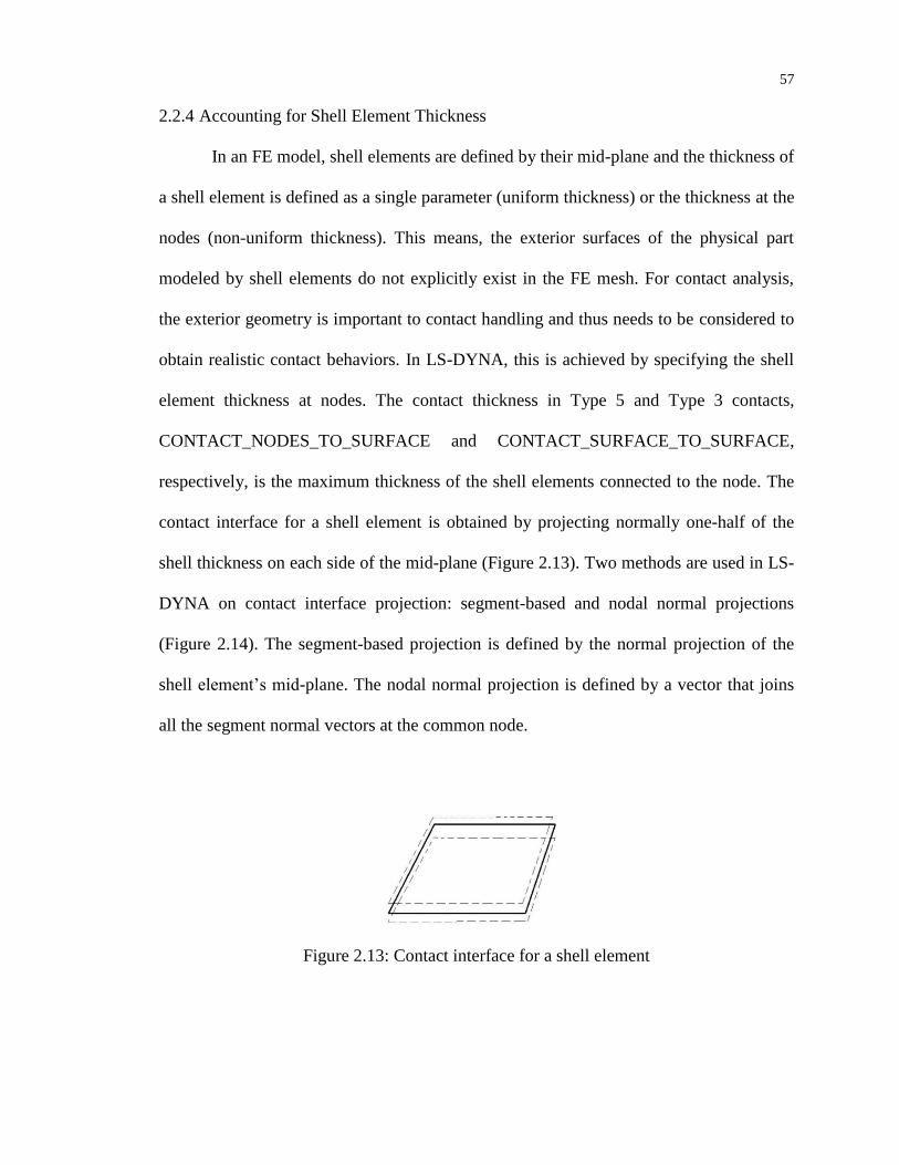
57
2.2.4 Accounting for Shell Element Thickness
In an FE model, shell elements are defined by their mid-plane and the thickness of
a shell element is defined as a single parameter (uniform thickness) or the thickness at the
nodes (non-uniform thickness). This means, the exterior surfaces of the physical part
modeled by shell elements do not explicitly exist in the FE mesh. For contact analysis,
the exterior geometry is important to contact handling and thus needs to be considered to
obtain realistic contact behaviors. In LS-DYNA, this is achieved by specifying the shell
element thickness at nodes. The contact thickness in Type 5 and Type 3 contacts,
CONTACT_NODES_TO_SURFACE and CONTACT_SURFACE_TO_SURFACE,
respectively, is the maximum thickness of the shell elements connected to the node. The
contact interface for a shell element is obtained by projecting normally one-half of the
shell thickness on each side of the mid-plane (Figure 2.13). Two methods are used in LS-
DYNA on contact interface projection: segment-based and nodal normal projections
(Figure 2.14). The segment-based projection is defined by the normal projection of the
shell element’s mid-plane. The nodal normal projection is defined by a vector that joins
all the segment normal vectors at the common node.
Figure 2.13: Contact interface for a shell element

58
a.
b.
Figure 2.14: Projected contact surfaces for shell elements using
a. Nodal normal projection; and b. segment based projection
In LS-DYNA, the CONTACT_AUTOMATIC_NODES_TO_SURFACE and
CONTACT_AUTOMATIC_SINGLE_SURFACE contacts use segment-based projection,
while other contact types use nodal normal projections if shell thickness is to be
considered in contacts. The main advantage of nodal normal projections is that a
continuous contact surface is obtained, as seen in Figure 2.14b. The disadvantages of
nodal projections are the increased cost on calculating the nodal normal vectors,
difficulty in treating T-intersections and geometric complications, and the need for
consistent orientation of contact segments. For example, the SINGLE_SURFACE contact,
which uses nodal normal projections, is slower than the
AUTOMATIC_SINGLE_SURFACE contact, which uses segment-based projections.
For contacts such as SINGLE_SURFACE, AUTOMATIC_SINGLE_SURFACE,
AUTOMATIC_GENERAL, and AUTOMATIC_GENERAL_INTERIOR, the default
contact thickness is chosen as the “shell thickness” or “40% of the shortest shell edge,”
whichever is smaller. This mechanism is based on past experience and usually works
except for situations where the in-plane dimension of a shell element is smaller than the
59
shell thickness. It prevents the usage of large, nonphysical contact thickness specified by
the users, which may considerably slow down the global contact searching algorithm.
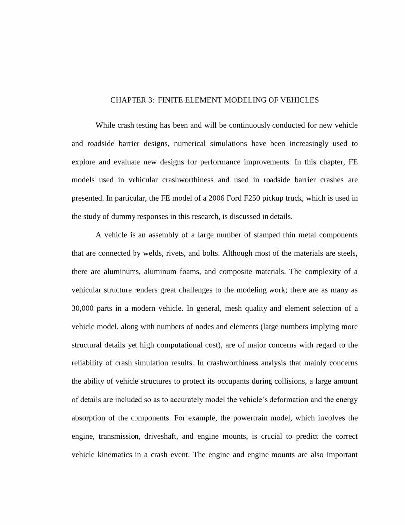
CHAPTER 3: FINITE ELEMENT MODELING OF VEHICLES
While crash testing has been and will be continuously conducted for new vehicle
and roadside barrier designs, numerical simulations have been increasingly used to
explore and evaluate new designs for performance improvements. In this chapter, FE
models used in vehicular crashworthiness and used in roadside barrier crashes are
presented. In particular, the FE model of a 2006 Ford F250 pickup truck, which is used in
the study of dummy responses in this research, is discussed in details.
A vehicle is an assembly of a large number of stamped thin metal components
that are connected by welds, rivets, and bolts. Although most of the materials are steels,
there are aluminums, aluminum foams, and composite materials. The complexity of a
vehicular structure renders great challenges to the modeling work; there are as many as
30,000 parts in a modern vehicle. In general, mesh quality and element selection of a
vehicle model, along with numbers of nodes and elements (large numbers implying more
structural details yet high computational cost), are of major concerns with regard to the
reliability of crash simulation results. In crashworthiness analysis that mainly concerns
the ability of vehicle structures to protect its occupants during collisions, a large amount
of details are included so as to accurately model the vehicle’s deformation and the energy
absorption of the components. For example, the powertrain model, which involves the
engine, transmission, driveshaft, and engine mounts, is crucial to predict the correct
vehicle kinematics in a crash event. The engine and engine mounts are also important

61
factors in determining the relative rotation between powertrain and body-in-white (Figure
3.1).
Figure 3.1: Body-in-white: a car body's sheet metal components welded together (URL4)
Unlike the vehicle models used in crashworthiness studies where a high degree of
complexity is required, vehicle models for roadside barrier crashes are often simplified in
the compartments and on the restraint systems. In addition, spot weld connections are
often modeled without failure mechanisms and rigid materials are often used wherever
deformation is considered small and negligible. With the advancement of computer
hardware and computational capacity, FE models of vehicles are now significantly
improved to include more details in order to capture realistic vehicle kinematics and
dynamic loading conditions encountered in a wide range of impact scenarios.
Over the years a number of different vehicle models have been selected,
developed and used by researchers worldwide. For example, many public available
vehicle models, from small passenger cars to pickup trucks, for the usage of median
barrier crash simulations have been developed in NCAC using reverse engineering
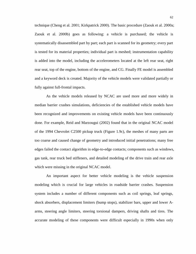
62
technique (Cheng et al. 2001; Kirkpatrick 2000). The basic procedure (Zaouk et al. 2000a;
Zaouk et al. 2000b) goes as following: a vehicle is purchased; the vehicle is
systematically disassembled part by part; each part is scanned for its geometry; every part
is tested for its material properties; individual part is meshed; instrumentation capability
is added into the model, including the accelerometers located at the left rear seat, right
rear seat, top of the engine, bottom of the engine, and CG. Finally FE model is assembled
and a keyword deck is created. Majority of the vehicle models were validated partially or
fully against full-frontal impacts.
As the vehicle models released by NCAC are used more and more widely in
median barrier crashes simulations, deficiencies of the established vehicle models have
been recognized and improvements on existing vehicle models have been continuously
done. For example, Reid and Marzougui (2002) found that in the original NCAC model
of the 1994 Chevrolet C2500 pickup truck (Figure 1.9c), the meshes of many parts are
too coarse and caused change of geometry and introduced initial penetrations; many free
edges failed the contact algorithm in edge-to-edge contacts; components such as windows,
gas tank, rear truck bed stiffeners, and detailed modeling of the drive train and rear axle
which were missing in the original NCAC model.
An important aspect for better vehicle modeling is the vehicle suspension
modeling which is crucial for large vehicles in roadside barrier crashes. Suspension
system includes a number of different components such as coil springs, leaf springs,
shock absorbers, displacement limiters (bump stops), stabilizer bars, upper and lower A-
arms, steering angle limiters, steering torsional dampers, driving shafts and tires. The
accurate modeling of these components were difficult especially in 1990s when only

63
some of the suspension components were modeled, less details of the geometries were
included and coarse meshes were used due to the limitation of computer power. For
example, Marzougui et al. (2003) and Marzougui et al. (2004) improved the rear
suspension of the 1994 Chevrolet C2500 pickup truck FE model by adding rear cross-
member, two complete leaf springs, two shock absorbers and hinges into the original
model and representing connections between suspension components such as hinges,
mountings and altering leaf spring constraints more realistically. Boesch and Reid (2005)
implemented a new front suspension and steering system for the same vehicle model, i.e.
the 1994 Chevrolet C2500 pickup truck FE model. In the new suspension system, a
deformable lower control arm with finer meshes were incorporated to capture the
deformation of the arm based on the observation that lower control arm failure, usually
either its joint or its deformation, is the most commonly failure in roadside crashes testing.
As more and more components have been incorporated and elements quality has been
greatly improved today, another fundamental difficulty, the lack of accurate structural
properties of suspension components due to the reluctance of vehicle manufactures to
provide that information (Tiso et al. 2002), is the bottleneck to accurate suspension
modeling. Researchers have been conducting more and more tests to obtain structural
properties of the suspension system (Mohan et al. 2009a). For example, in the research
efforts on improving suspension modeling of a 1994 Chevrolet C2500 pickup truck, Tiso
et al. (2002) carried out many simple tests such as coil spring compression, leaf spring
compression and rebounding, front and rear suspension roll-off drop tests, steering wheel
rotation (by a constant torque), and vehicle running over a curb. Testing is still very
limited due to lack of equipment and experimental difficulty.

64
Tire is a very important component to provide suspension and has a direct role in
affecting vehicle trajectory. Unlike simulation practice in tire industry, a very detailed tire
model (Ghoreishy 2008; Steen 2007) is too expensive computationally to be incorporated
as part of a complete vehicle model in median barrier crashes. On the other hand, a less
detailed tire may show a considerable sensitivity to the tire properties (Tiso et al. 2002).
Balance should be achieved between model performance and model details. In vehicle
modeling practice at NCAC, the tire is usually modeled as a layer of shell elements with
uniform thickness along with isotropic elastic material. A simple airbag model provided
by LS-DYNA is used for internal pressure modeling. Although simple and
computationally efficient its drawbacks are obvious including mesh tangling when
enveloping obstacles, unrealistic cupping, inability to deform to a plane surface in the
contact patch region, and inability to capture tire failure modes (flat tire caused by tire
debedding, tire pinching against the flange of the rim and rupture of the tire due to impact
with an object such as a guardrail post). To address the issue of flat tire caused by tire
debedding, Orengo et al. (2003) developed a tire model for the NCAC 1994 Chevrolet
C2500 pickup model using solid elements modeling tread, shell elements modeling the
sidewall and the bead coils, beam elements modeling the radial reinforcement fibers.
Realizing available tire models inadequately capture tire behavior where tire encounters
large bumps, such as a culvert grate, a pothole, or curbs, Reid et al. (2007) used solid
elements for the tread, shell elements for the sidewall, and beam elements for the bead,
steel belts, and body plies; different material properties for different components,
sidewall thickness variation and numerical damping to remove unrealistic tire vibration
were also considered.

65
3.1 FE Model of a 2006 Ford F250 Pickup Truck
The FE model of a 2006 Ford F250 Pickup Truck (see Figure 3.2), which was
initially developed by NCAC, was used to evaluate the dummy responses in simulations
of roadside crash crashes. This vehicle model was only validated by NCAC using a full-
frontal impact test, and exhibited numerical instability in barrier crash simulations. To
use it in the research work of this dissertation, this model was revised to improve the
numerical stability and ultimately simulation accuracy. The revised vehicle model was
validated using experimental data of a full-frontal and a 40% offset frontal impact tests
conducted by NTHSA.
The details of the modeling work on the original Ford F250 was provided by
Opiela et al. (2008b) including components testing and validation. This FE model had
738,165 nodes, 698,501 shell elements, 2,353 beam elements, and 25,905 solid elements.
The steering (excluding steering wheel) and suspension components were modeled but
some compartment components, e.g., the seat and dashboard, and the restraint systems
were not included. The mass of the vehicle was approximated 3,000 kg, which met the
requirements of a 2270P (pickup truck) test vehicle specified by the MASH for the Test
Level 3 (TL-3) impact conditions (i.e., with an impact speed of 100 km/hr and a 25°
impact angle).

66
Figure 3.2: The NCAC FE model of a 2006 Ford F250 pickup truck (Opiela et al. 2008b)
3.1.1 Simulation of a Full-frontal Impact Test
The NCAC FE model of the Ford F250 was validated against full-frontal impact
tests conducted by the Transportation Research Center Inc. (TRC 2006). Comparisons
were made between simulation results and test data on impact forces, accelerations, etc.
The total impact duration simulated was 200 ms, which was sufficient to cover the whole
impact event.
The energy needed to be conserved throughout the simulations. No significant
energy loss or gain should be observed in numerical simulations. In LS-DYNA the
energy conservation is measured by a so-called energy ratio defined as
0 0
W t
W Wt
t
(3.1)
where is the total energy at any time t, is the work done by external forces,
and is the total energy at time t = 0. If the energy is well conserved, the energy
ratio will be ideally 1.0 at every time instant, i.e. . In the full-frontal impact
simulation using the NCAC model, the variation of energy ratio was found less than 0.7%

67
(Figure 3.3), which indicated that the total energy was well conserved in the numerical
simulation.
Figure 3.3: Energy ratio by the NCAC FE model in a full-frontal impact simulation with
a time-step of 0.5 ms
The impact forces served as an important factor that indicated the accuracy of the
contact algorithm being used as well as affected the overall vehicle impact consequences.
In the frontal impact simulation using the NCAC model, the time history of impact forces
matched with experimental data reasonably well, as shown in Figure 3.4. The first peak
force agreed well regarding both magnitude and timing.
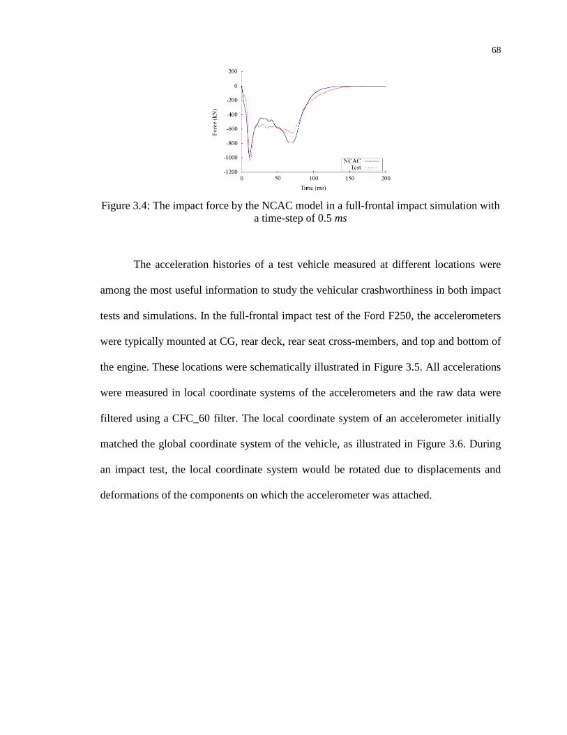
68
Figure 3.4: The impact force by the NCAC model in a full-frontal impact simulation with
a time-step of 0.5 ms
The acceleration histories of a test vehicle measured at different locations were
among the most useful information to study the vehicular crashworthiness in both impact
tests and simulations. In the full-frontal impact test of the Ford F250, the accelerometers
were typically mounted at CG, rear deck, rear seat cross-members, and top and bottom of
the engine. These locations were schematically illustrated in Figure 3.5. All accelerations
were measured in local coordinate systems of the accelerometers and the raw data were
filtered using a CFC_60 filter. The local coordinate system of an accelerometer initially
matched the global coordinate system of the vehicle, as illustrated in Figure 3.6. During
an impact test, the local coordinate system would be rotated due to displacements and
deformations of the components on which the accelerometer was attached.
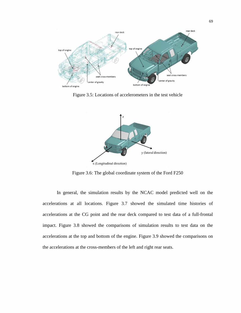
69
Figure 3.5: Locations of accelerometers in the test vehicle
Figure 3.6: The global coordinate system of the Ford F250
In general, the simulation results by the NCAC model predicted well on the
accelerations at all locations. Figure 3.7 showed the simulated time histories of
accelerations at the CG point and the rear deck compared to test data of a full-frontal
impact. Figure 3.8 showed the comparisons of simulation results to test data on the
accelerations at the top and bottom of the engine. Figure 3.9 showed the comparisons on
the accelerations at the cross-members of the left and right rear seats.

70
a. b.
Figure 3.7: The time histories of accelerations along the longitudinal direction by the
NCAC model with a time-step of 0.5 ms
a. At CG point; and b. at rear deck
a. b.
Figure 3.8: The time histories of accelerations along the longitudinal direction by the
NCAC model with a time-step of 0.5 ms
a. At top of the engine; and b. at bottom of the engine
a. b.
Figure 3.9: The time histories of accelerations along the longitudinal direction by the
NCAC model with a time-step of 0.5 ms at cross-member of
a. Left rear seat; and b. right rear seat

71
The comparison of simulation results to test data showed the NCAC model had
reasonably good overall prediction of the test results. One way to further improve the
NCAC model on its numerical stability in roadside barrier crash simulations is to
decrease the time-step such that no mass scaling is invoked, e.g., from 0.5 ms to 0.1 ms.
Comparisons of the simulation results by the NCAC model with a time-step of 0.1 ms
with test data were shown in Figure 3.10 to Figure 3.15. The comparisons showed that
some simulation results became worse with a decreased time-step. This observation
confirmed the existence of some deficiencies in the NCAC model that needed to be
improved before used in roadside barrier crash simulations.
Figure 3.10: Energy ratio by the NCAC FE model in a full-frontal impact simulation with
a time-step of 0.1 ms
Figure 3.11: The impact force by the NCAC model in a full-frontal impact simulation
with a time-step of 0.1 ms
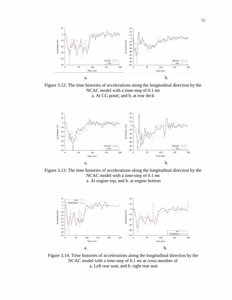
72
a. b.
Figure 3.12: The time histories of accelerations along the longitudinal direction by the
NCAC model with a time-step of 0.1 ms
a. At CG point; and b. at rear deck
a. b.
Figure 3.13: The time histories of accelerations along the longitudinal direction by the
NCAC model with a time-step of 0.1 ms
a. At engine top; and b. at engine bottom
a. b.
Figure 3.14: Time histories of accelerations along the longitudinal direction by the
NCAC model with a time-step of 0.1 ms at cross member of
a. Left rear seat; and b. right rear seat

73
The decreased accuracy of simulation results implied that the model had
instability issues, and one major source of this instability was the contact instability,
which could be reflected by contact energy given by
1
21
1 1
nnsn nmn
n n s s m m
c c i i i i
i i
E E F d F d
(3.2)
where
are the number of nodes, nodal force and nodal displacements,
respectively, on slave surface;
are the number of nodes nodal force and
nodal displacements, respectively, on master surface; and
are the contact
energy at time-step n + 1 and time step n. Without concerning about frictions, the
calculated contact energy should ideally be zero or be small enough. With the presence of
frictions, however, as are the case with most engineering problems, contact energy is
essentially the energy done by friction forces and should be always be positive and zero
or negative value indicates undetected penetrations or failure in contact handling.
For the NCAC model, the contact energy from simulations with different time-
steps was found inconsistent, as shown in Figure 3.15. The contact energy became
negative in the simulation with a decreased time-step; this indicated that contact
penetrations occurred in the simulation and deteriorated the simulation credibility.
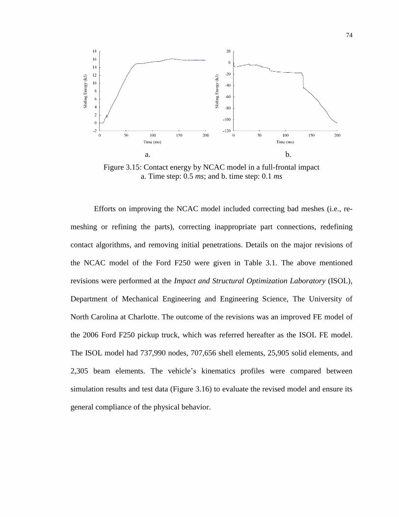
74
a. b.
Figure 3.15: Contact energy by NCAC model in a full-frontal impact
a. Time step: 0.5 ms; and b. time step: 0.1 ms
Efforts on improving the NCAC model included correcting bad meshes (i.e., re-
meshing or refining the parts), correcting inappropriate part connections, redefining
contact algorithms, and removing initial penetrations. Details on the major revisions of
the NCAC model of the Ford F250 were given in Table 3.1. The above mentioned
revisions were performed at the Impact and Structural Optimization Laboratory (ISOL),
Department of Mechanical Engineering and Engineering Science, The University of
North Carolina at Charlotte. The outcome of the revisions was an improved FE model of
the 2006 Ford F250 pickup truck, which was referred hereafter as the ISOL FE model.
The ISOL model had 737,990 nodes, 707,656 shell elements, 25,905 solid elements, and
2,305 beam elements. The vehicle’s kinematics profiles were compared between
simulation results and test data (Figure 3.16) to evaluate the revised model and ensure its
general compliance of the physical behavior.
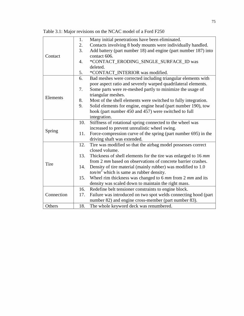
75
Table 3.1: Major revisions on the NCAC model of a Ford F250
Contact
1. Many initial penetrations have been eliminated.
2. Contacts involving 8 body mounts were individually handled.
3. Add battery (part number 18) and engine (part number 187) into
contact 606.
4. *CONTACT_ERODING_SINGLE_SURFACE_ID was
deleted.
5. *CONTACT_INTERIOR was modified.
Elements
6. Bad meshes were corrected including triangular elements with
poor aspect ratio and severely warped quadrilateral elements.
7. Some parts were re-meshed partly to minimize the usage of
triangular meshes.
8. Most of the shell elements were switched to fully integration.
9. Solid elements for engine, engine head (part number 190), tow
hook (part number 450 and 457) were switched to full
integration.
Spring
10. Stiffness of rotational spring connected to the wheel was
increased to prevent unrealistic wheel swing.
11. Force-compression curve of the spring (part number 695) in the
driving shaft was extended.
Tire
12. Tire was modified so that the airbag model possesses correct
closed volume.
13. Thickness of shell elements for the tire was enlarged to 16 mm
from 2 mm based on observations of concrete barrier crashes.
14. Density of tire material (mainly rubber) was modified to 1.0
ton/m3 which is same as rubber density.
15. Wheel rim thickness was changed to 6 mm from 2 mm and its
density was scaled down to maintain the right mass.
Connection
16. Redefine belt tensioner constraints to engine block.
17. Failure was introduced on two spot welds connecting hood (part
number 82) and engine cross-member (part number 83).
Others 18. The whole keyword deck was renumbered.
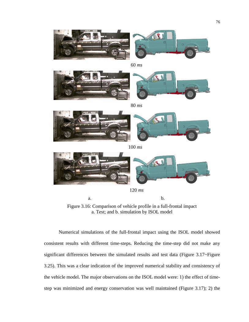
76
60 ms
80 ms
100 ms
120 ms
a. b.
Figure 3.16: Comparison of vehicle profile in a full-frontal impact
a. Test; and b. simulation by ISOL model
Numerical simulations of the full-frontal impact using the ISOL model showed
consistent results with different time-steps. Reducing the time-step did not make any
significant differences between the simulated results and test data (Figure 3.17~Figure
3.25). This was a clear indication of the improved numerical stability and consistency of
the vehicle model. The major observations on the ISOL model were: 1) the effect of time-
step was minimized and energy conservation was well maintained (Figure 3.17); 2) the

77
prediction on the impact force was improved (Figure 3.19); 3) the negative sliding energy
was significantly reduced (Figure 3.18); 4) the prediction on the CG acceleration was
greatly improved, e.g., the accurate capture of the first peak (Figure 3.20); 5) the
accelerations at the engine top (Figure 3.21) and engine bottom (Figure 3.22) were
improved; and 6) the first peak acceleration on the cross-member of the left rear seat was
well captured regardless of the time-steps used (Figure 3.24), and the same was true for
the accelerations on the cross-member of the right rear seat (Figure 3.25).
a. b.
Figure 3.17: Energy ratio by the ISOL model
a. Time step: 0.5 ms; and b. time step 0.1 ms
a. b.
Figure 3.18: Contact energy by the ISOL model
a. Time step: 0.5 ms; and b. time step: 0.1 ms
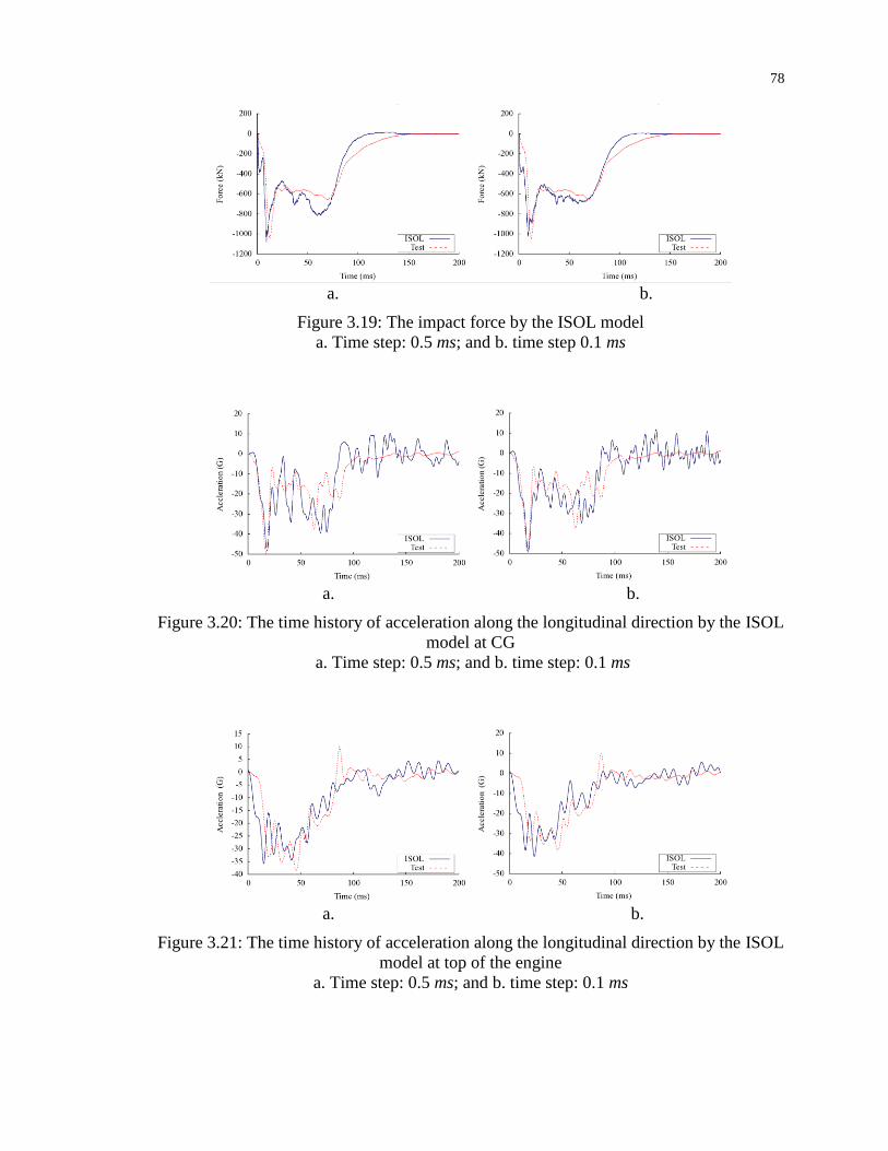
78
a. b.
Figure 3.19: The impact force by the ISOL model
a. Time step: 0.5 ms; and b. time step 0.1 ms
a. b.
Figure 3.20: The time history of acceleration along the longitudinal direction by the ISOL
model at CG
a. Time step: 0.5 ms; and b. time step: 0.1 ms
a. b.
Figure 3.21: The time history of acceleration along the longitudinal direction by the ISOL
model at top of the engine
a. Time step: 0.5 ms; and b. time step: 0.1 ms
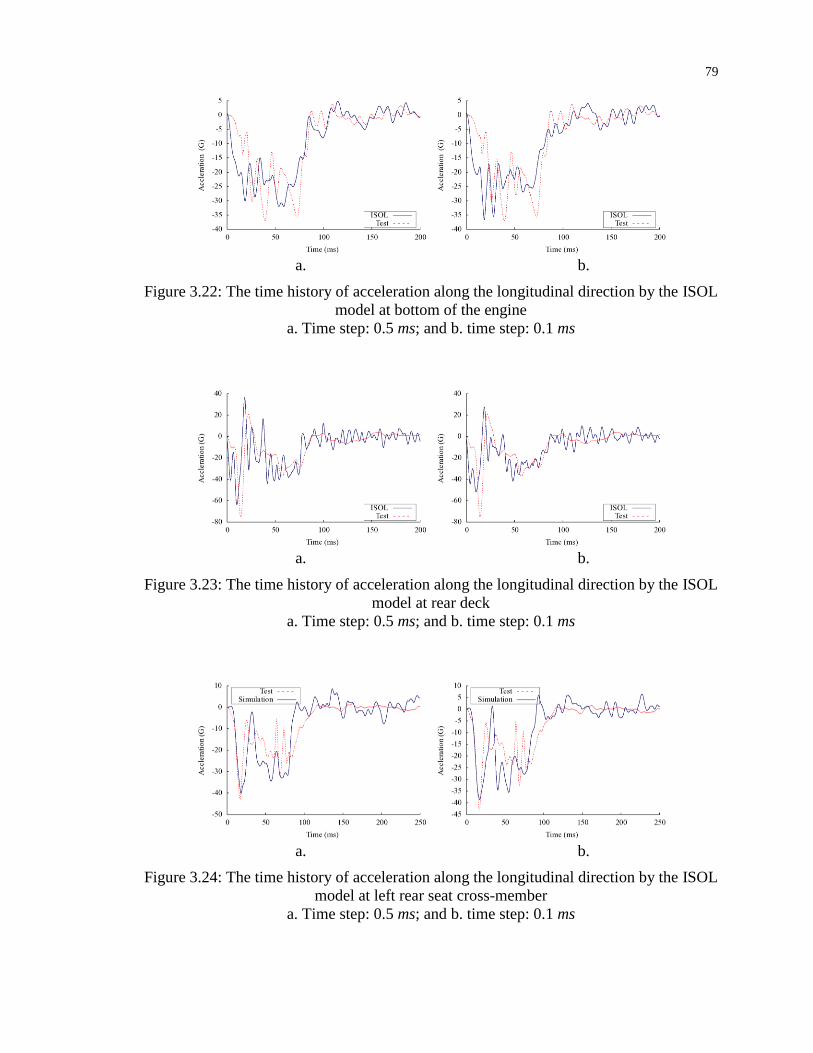
79
a. b.
Figure 3.22: The time history of acceleration along the longitudinal direction by the ISOL
model at bottom of the engine
a. Time step: 0.5 ms; and b. time step: 0.1 ms
a. b.
Figure 3.23: The time history of acceleration along the longitudinal direction by the ISOL
model at rear deck
a. Time step: 0.5 ms; and b. time step: 0.1 ms
a. b.
Figure 3.24: The time history of acceleration along the longitudinal direction by the ISOL
model at left rear seat cross-member
a. Time step: 0.5 ms; and b. time step: 0.1 ms

80
a. b.
Figure 3.25: The time history of acceleration along the longitudinal direction by the ISOL
model at right rear seat cross-member
a. Time step: 0.5 ms; and b. time step: 0.1 ms
3.1.2 Simulation of an Offset Frontal Impact Test
In an offset-frontal impact test, the deformation and the energy absorption are
more localized thus more challenging to the modeling work than in a full-frontal impact
test. The original NCAC model was not validated by an offset frontal impact test, which
would impose more demands on the robustness of the FE model of a vehicle and
structural components than the full-frontal impact test. In this section, the ISOL model of
the Ford F250 will be examined against an offset-frontal impact test conducted by the
Transportation Research Center Inc. (TRC 2007).
In an offset frontal impact, the vehicle impacts a deformable barrier made of
aluminum honeycomb (Figure 3.26) at an impact speed of 64.4 km/hr (40 mph), which is
higher than the impact speed of 56.3 km/hr (35 mph) in a full-frontal impact. Modeling
the deformable barrier added extra difficulties to the offset frontal impact simulation. A
popular and cost effective way to model this barrier was to model the cellular foam as
continuum solids assigned with equivalent bulk properties. An LS-DYNA FE model of
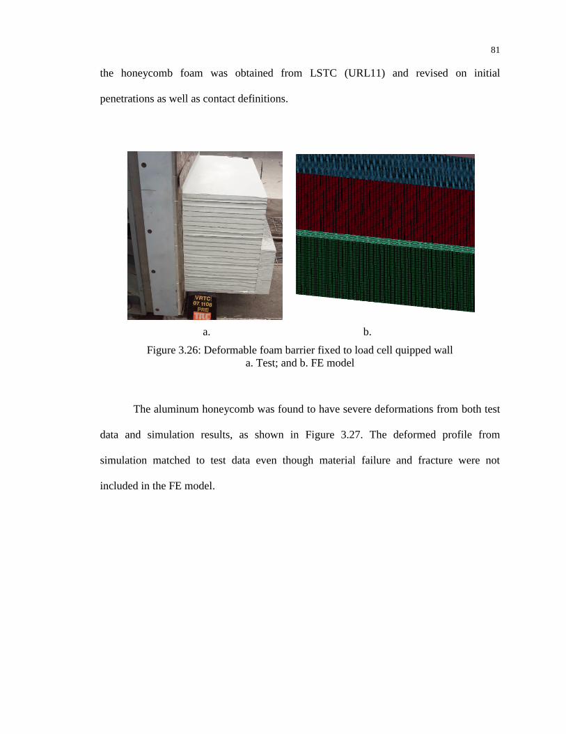
81
the honeycomb foam was obtained from LSTC (URL11) and revised on initial
penetrations as well as contact definitions.
a. b.
Figure 3.26: Deformable foam barrier fixed to load cell quipped wall
a. Test; and b. FE model
The aluminum honeycomb was found to have severe deformations from both test
data and simulation results, as shown in Figure 3.27. The deformed profile from
simulation matched to test data even though material failure and fracture were not
included in the FE model.

82
a. b.
c. d.
Figure 3.27: Deformed ODB in impact test (TRC 2007)
a. Side view in test; b. front view in test; c. side view in simulation; and d. front view in
simulation
Significant vehicular deformations were observed in the offset frontal impact test
shown in Figure 3.28. The front-left corner of the pickup truck severely deformed and the
suspension was damaged. The doors on the driver side were compressed and forced to
open up in the test. The simulation results using the ISOL model were compared to test
data at the same time instances, as shown in Figure 3.29.
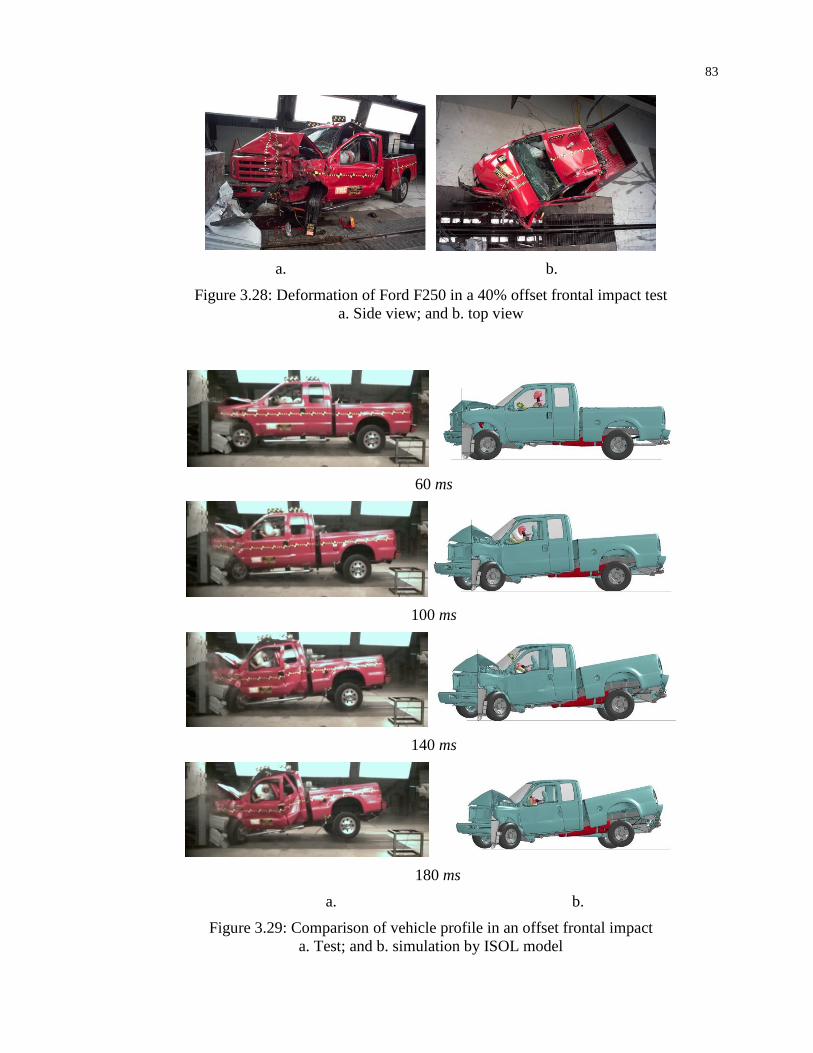
83
a. b.
Figure 3.28: Deformation of Ford F250 in a 40% offset frontal impact test
a. Side view; and b. top view
60 ms
100 ms
140 ms
180 ms
a. b.
Figure 3.29: Comparison of vehicle profile in an offset frontal impact
a. Test; and b. simulation by ISOL model
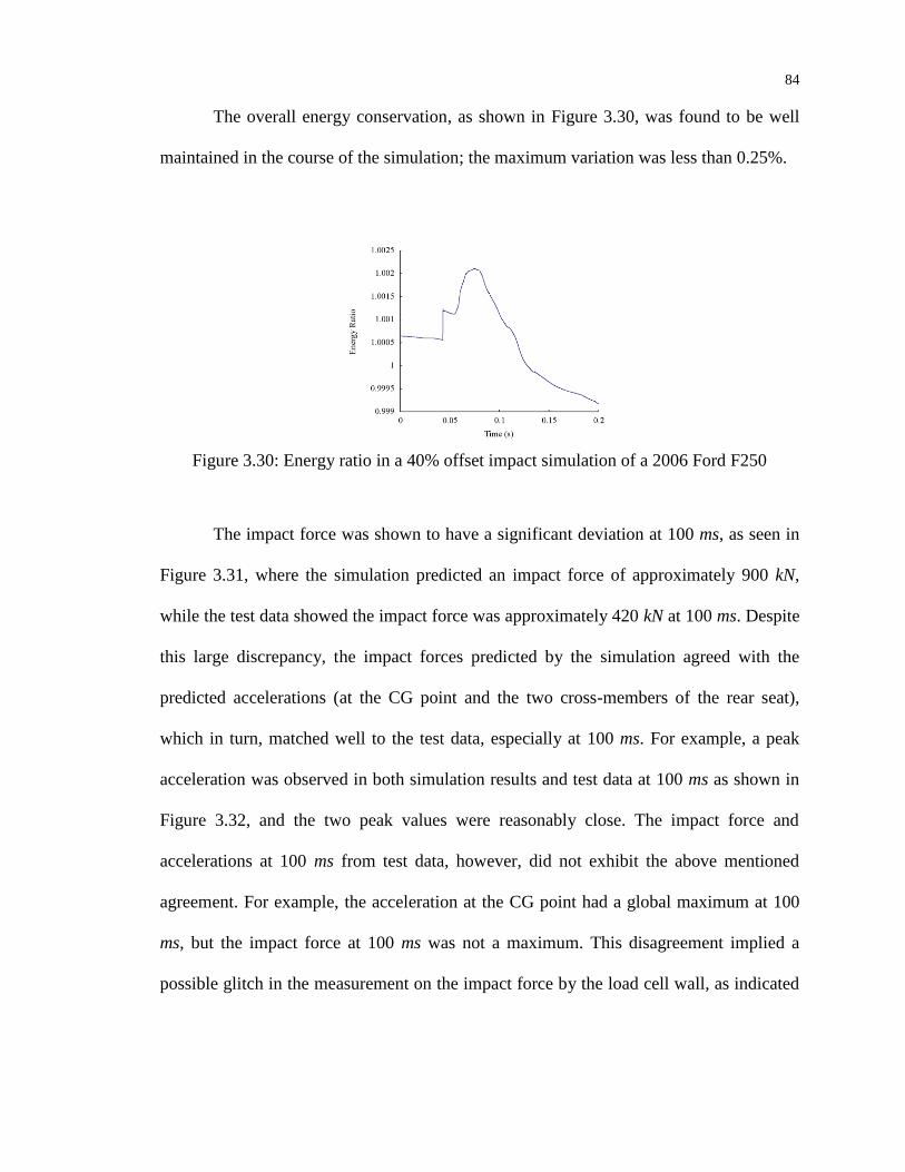
84
The overall energy conservation, as shown in Figure 3.30, was found to be well
maintained in the course of the simulation; the maximum variation was less than 0.25%.
Figure 3.30: Energy ratio in a 40% offset impact simulation of a 2006 Ford F250
The impact force was shown to have a significant deviation at 100 ms, as seen in
Figure 3.31, where the simulation predicted an impact force of approximately 900 kN,
while the test data showed the impact force was approximately 420 kN at 100 ms. Despite
this large discrepancy, the impact forces predicted by the simulation agreed with the
predicted accelerations (at the CG point and the two cross-members of the rear seat),
which in turn, matched well to the test data, especially at 100 ms. For example, a peak
acceleration was observed in both simulation results and test data at 100 ms as shown in
Figure 3.32, and the two peak values were reasonably close. The impact force and
accelerations at 100 ms from test data, however, did not exhibit the above mentioned
agreement. For example, the acceleration at the CG point had a global maximum at 100
ms, but the impact force at 100 ms was not a maximum. This disagreement implied a
possible glitch in the measurement on the impact force by the load cell wall, as indicated
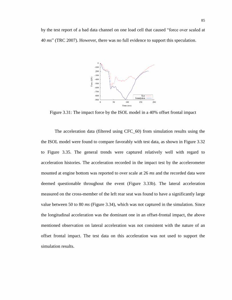
85
by the test report of a bad data channel on one load cell that caused “force over scaled at
40 ms” (TRC 2007). However, there was no full evidence to support this speculation.
Figure 3.31: The impact force by the ISOL model in a 40% offset frontal impact
The acceleration data (filtered using CFC_60) from simulation results using the
the ISOL model were found to compare favorably with test data, as shown in Figure 3.32
to Figure 3.35. The general trends were captured relatively well with regard to
acceleration histories. The acceleration recorded in the impact test by the accelerometer
mounted at engine bottom was reported to over scale at 26 ms and the recorded data were
deemed questionable throughout the event (Figure 3.33b). The lateral acceleration
measured on the cross-member of the left rear seat was found to have a significantly large
value between 50 to 80 ms (Figure 3.34), which was not captured in the simulation. Since
the longitudinal acceleration was the dominant one in an offset-frontal impact, the above
mentioned observation on lateral acceleration was not consistent with the nature of an
offset frontal impact. The test data on this acceleration was not used to support the
simulation results.
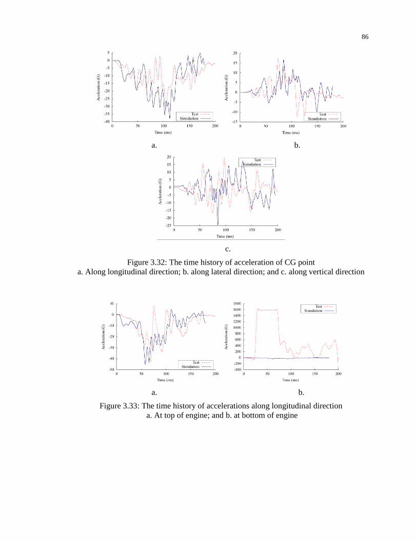
86
a. b.
c.
Figure 3.32: The time history of acceleration of CG point
a. Along longitudinal direction; b. along lateral direction; and c. along vertical direction
a. b.
Figure 3.33: The time history of accelerations along longitudinal direction
a. At top of engine; and b. at bottom of engine

87
a. b.
Figure 3.34: The time history of acceleration of left rear seat cross-member
a. Along longitudinal direction; and b. along lateral direction
a. b.
Figure 3.35: The time history of acceleration of right rear seat cross-member
a. Along longitudinal direction; and b. along lateral direction
3.2 FE Model of the Passive Restraint System
The passive restraint system, including the airbag, collapsible steering column,
and seatbelt, is important to protect the passenger in a crash event. Although it does not
contribute significantly to the overall vehicle behavior or response, the passive restraint
system is critical to reduce the impact forces and accelerations on the occupant. Nearly
all the vehicle models developed by NCAC had no passive restraint system; this made it
impossible to incorporate an occupant (dummy) model into the vehicle model to study
occupant responses in roadway crashes. In this dissertation research, the FE models of the
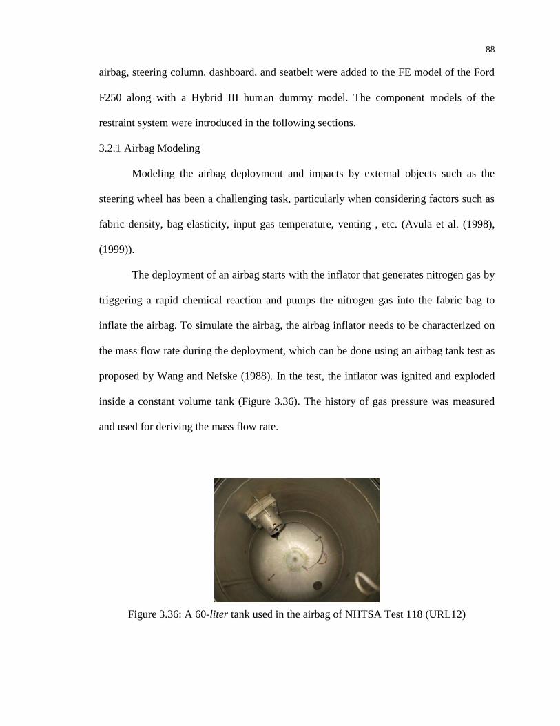
88
airbag, steering column, dashboard, and seatbelt were added to the FE model of the Ford
F250 along with a Hybrid III human dummy model. The component models of the
restraint system were introduced in the following sections.
3.2.1 Airbag Modeling
Modeling the airbag deployment and impacts by external objects such as the
steering wheel has been a challenging task, particularly when considering factors such as
fabric density, bag elasticity, input gas temperature, venting , etc. (Avula et al. (1998),
(1999)).
The deployment of an airbag starts with the inflator that generates nitrogen gas by
triggering a rapid chemical reaction and pumps the nitrogen gas into the fabric bag to
inflate the airbag. To simulate the airbag, the airbag inflator needs to be characterized on
the mass flow rate during the deployment, which can be done using an airbag tank test as
proposed by Wang and Nefske (1988). In the test, the inflator was ignited and exploded
inside a constant volume tank (Figure 3.36). The history of gas pressure was measured
and used for deriving the mass flow rate.
Figure 3.36: A 60-liter tank used in the airbag of NHTSA Test 118 (URL12)
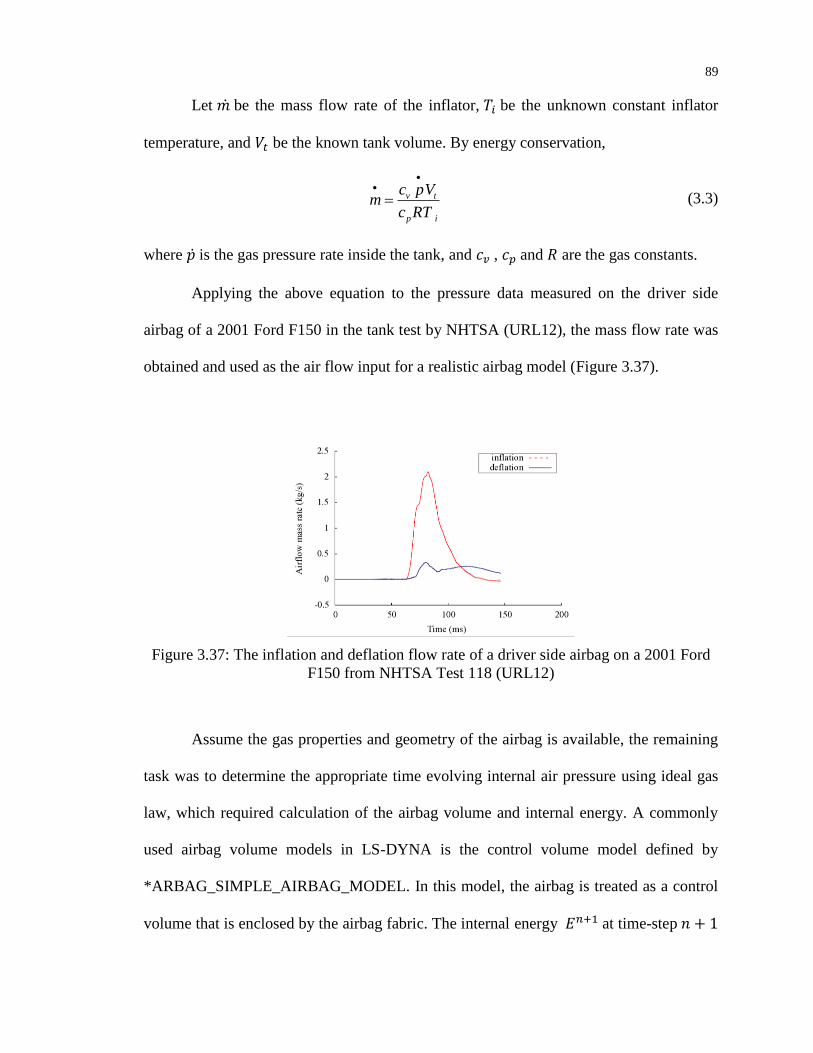
89
Let ̇ be the mass flow rate of the inflator, be the unknown constant inflator
temperature, and be the known tank volume. By energy conservation,
v t
p i
c pVm
c RT
(3.3)
where ̇ is the gas pressure rate inside the tank, and , and are the gas constants.
Applying the above equation to the pressure data measured on the driver side
airbag of a 2001 Ford F150 in the tank test by NHTSA (URL12), the mass flow rate was
obtained and used as the air flow input for a realistic airbag model (Figure 3.37).
Figure 3.37: The inflation and deflation flow rate of a driver side airbag on a 2001 Ford
F150 from NHTSA Test 118 (URL12)
Assume the gas properties and geometry of the airbag is available, the remaining
task was to determine the appropriate time evolving internal air pressure using ideal gas
law, which required calculation of the airbag volume and internal energy. A commonly
used airbag volume models in LS-DYNA is the control volume model defined by
*ARBAG_SIMPLE_AIRBAG_MODEL. In this model, the airbag is treated as a control
volume that is enclosed by the airbag fabric. The internal energy at time-step
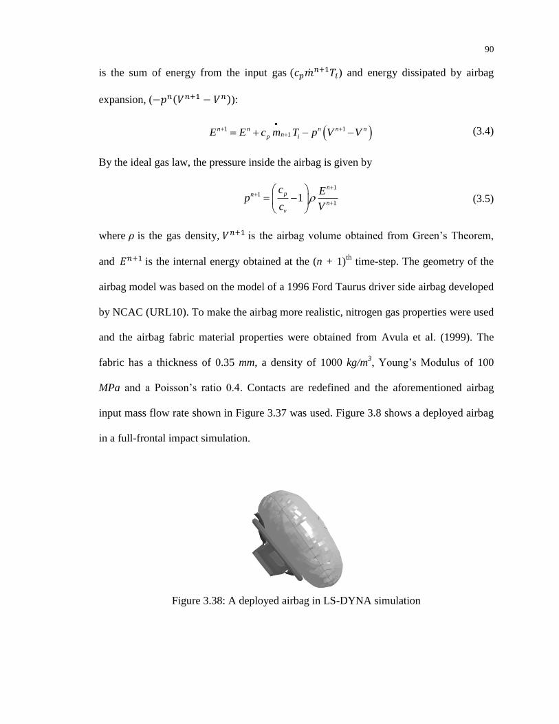
90
is the sum of energy from the input gas ̇ ) and energy dissipated by airbag
expansion, ( ):
1 1
1n n n n n
np iE E c m T p V V
(3.4)
By the ideal gas law, the pressure inside the airbag is given by
11
11
npn
n
v
c Ep
c V
(3.5)
where is the gas density, is the airbag volume obtained from Green’s Theorem,
and is the internal energy obtained at the (n + 1)th
time-step. The geometry of the
airbag model was based on the model of a 1996 Ford Taurus driver side airbag developed
by NCAC (URL10). To make the airbag more realistic, nitrogen gas properties were used
and the airbag fabric material properties were obtained from Avula et al. (1999). The
fabric has a thickness of 0.35 mm, a density of 1000 kg/m3, Young’s Modulus of 100
MPa and a Poisson’s ratio 0.4. Contacts are redefined and the aforementioned airbag
input mass flow rate shown in Figure 3.37 was used. Figure 3.8 shows a deployed airbag
in a full-frontal impact simulation.
Figure 3.38: A deployed airbag in LS-DYNA simulation
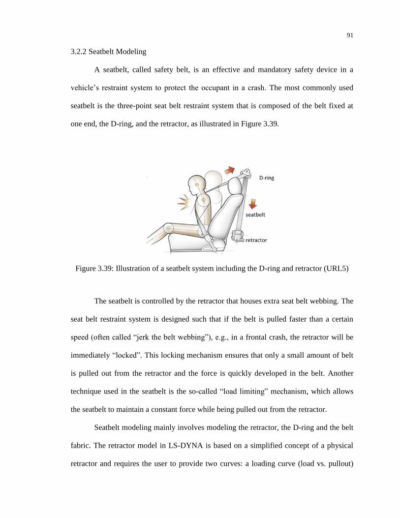
91
3.2.2 Seatbelt Modeling
A seatbelt, called safety belt, is an effective and mandatory safety device in a
vehicle’s restraint system to protect the occupant in a crash. The most commonly used
seatbelt is the three-point seat belt restraint system that is composed of the belt fixed at
one end, the D-ring, and the retractor, as illustrated in Figure 3.39.
Figure 3.39: Illustration of a seatbelt system including the D-ring and retractor (URL5)
The seatbelt is controlled by the retractor that houses extra seat belt webbing. The
seat belt restraint system is designed such that if the belt is pulled faster than a certain
speed (often called “jerk the belt webbing”), e.g., in a frontal crash, the retractor will be
immediately “locked”. This locking mechanism ensures that only a small amount of belt
is pulled out from the retractor and the force is quickly developed in the belt. Another
technique used in the seatbelt is the so-called “load limiting” mechanism, which allows
the seatbelt to maintain a constant force while being pulled out from the retractor.
Seatbelt modeling mainly involves modeling the retractor, the D-ring and the belt
fabric. The retractor model in LS-DYNA is based on a simplified concept of a physical
retractor and requires the user to provide two curves: a loading curve (load vs. pullout)

92
and an unloading curve (load vs. payout). The terms pullout and payout are defined as the
amount of belt length extracted from the retractor. The seatbelt force is determined by the
load curve based on the amount of pullout (Figure 3.40). In a simulation, the retractor is
initially unlocked with a constant tensile force. Any slack in the belt is eaten up to
maintain a tightened belt.
Figure 3.40: The loading curve for seatbelt retractor in a frontal impact simulation
The D-ring is modeled by a slipring element in LS-DYNA with no geometric
representation of the physical ring (Figure 3.41). The slipring element is essentially a
nodal point attached or fixed to the vehicle’s frame. No belt slip will occur if the forces in
the belt on both sides of the ring satisfy the following equilibrium condition:
1
2
Te
T
(3.6)
where is and are the belt forces, is the friction coefficient between the belt and D-
ring, and is the wrap angle. The friction coefficient is the only parameter needs to be
provided by user; the wrap angle is calculated during the simulation based on the belt
positions.
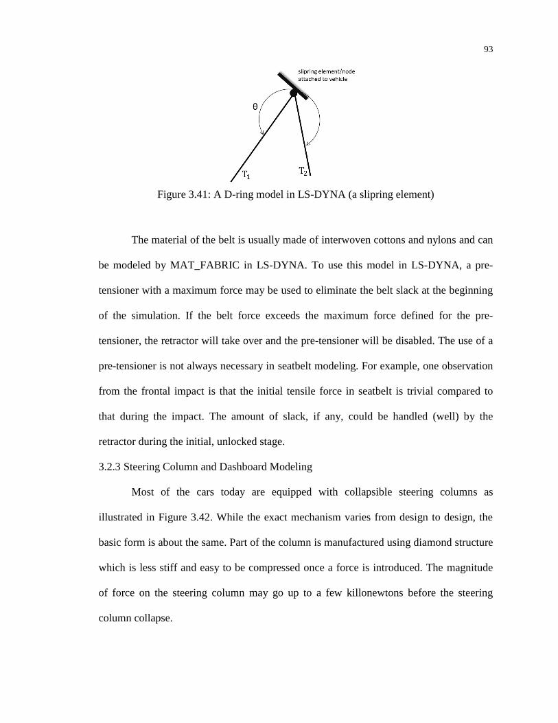
93
Figure 3.41: A D-ring model in LS-DYNA (a slipring element)
The material of the belt is usually made of interwoven cottons and nylons and can
be modeled by MAT_FABRIC in LS-DYNA. To use this model in LS-DYNA, a pre-
tensioner with a maximum force may be used to eliminate the belt slack at the beginning
of the simulation. If the belt force exceeds the maximum force defined for the pre-
tensioner, the retractor will take over and the pre-tensioner will be disabled. The use of a
pre-tensioner is not always necessary in seatbelt modeling. For example, one observation
from the frontal impact is that the initial tensile force in seatbelt is trivial compared to
that during the impact. The amount of slack, if any, could be handled (well) by the
retractor during the initial, unlocked stage.
3.2.3 Steering Column and Dashboard Modeling
Most of the cars today are equipped with collapsible steering columns as
illustrated in Figure 3.42. While the exact mechanism varies from design to design, the
basic form is about the same. Part of the column is manufactured using diamond structure
which is less stiff and easy to be compressed once a force is introduced. The magnitude
of force on the steering column may go up to a few killonewtons before the steering
column collapse.
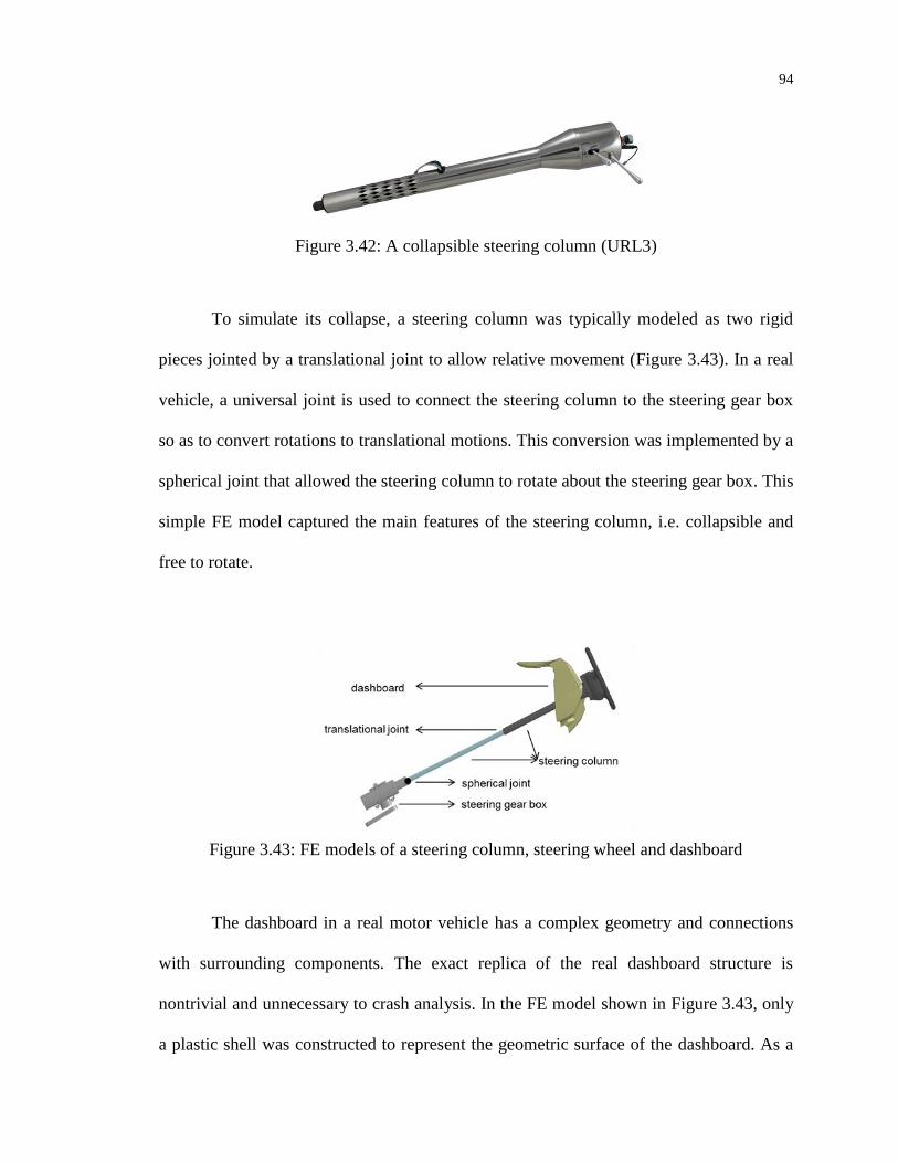
94
Figure 3.42: A collapsible steering column (URL3)
To simulate its collapse, a steering column was typically modeled as two rigid
pieces jointed by a translational joint to allow relative movement (Figure 3.43). In a real
vehicle, a universal joint is used to connect the steering column to the steering gear box
so as to convert rotations to translational motions. This conversion was implemented by a
spherical joint that allowed the steering column to rotate about the steering gear box. This
simple FE model captured the main features of the steering column, i.e. collapsible and
free to rotate.
Figure 3.43: FE models of a steering column, steering wheel and dashboard
The dashboard in a real motor vehicle has a complex geometry and connections
with surrounding components. The exact replica of the real dashboard structure is
nontrivial and unnecessary to crash analysis. In the FE model shown in Figure 3.43, only
a plastic shell was constructed to represent the geometric surface of the dashboard. As a

95
result of this simplification, the dashboard deformation from simulation results was not
expected to have an exact match to that observed in a crash test.
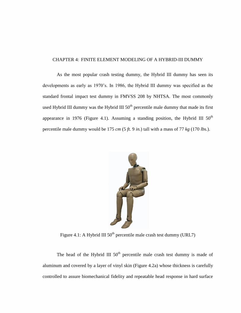
CHAPTER 4: FINITE ELEMENT MODELING OF A HYBRID-III DUMMY
As the most popular crash testing dummy, the Hybrid III dummy has seen its
developments as early as 1970’s. In 1986, the Hybrid III dummy was specified as the
standard frontal impact test dummy in FMVSS 208 by NHTSA. The most commonly
used Hybrid III dummy was the Hybrid III 50th
percentile male dummy that made its first
appearance in 1976 (Figure 4.1). Assuming a standing position, the Hybrid III 50th
percentile male dummy would be 175 cm (5 ft. 9 in.) tall with a mass of 77 kg (170 lbs.).
Figure 4.1: A Hybrid III 50th
percentile male crash test dummy (URL7)
The head of the Hybrid III 50th
percentile male crash test dummy is made of
aluminum and covered by a layer of vinyl skin (Figure 4.2a) whose thickness is carefully
controlled to assure biomechanical fidelity and repeatable head response in hard surface

97
impact (Mertz 1985). The neck has three rigid aluminum vertebral elements which are
molded in a high damping butyl elastomer (Figure 4.2b). A single steel cable runs
through the center of the neck to provide the axial strength. An asymmetrical cross-
sectional geometry provides the bending resistance to match the biomechanics data. Cuts
on the anterior half further reduces the extension bending resistance without affecting the
flexion response (Culver et al. 1972). The thorax (Figure 4.2c) consists of a spine and rib
cage (six steel ribs) covered by a removable chest flesh and skin assembly (often referred
as the jacket). A viscous damping material is bonded to the internal surfaces of the ribs. A
urethane bib is attached to the front sides of the ribs to help distribute the loads (Horsch
and Schneider 1988). The lumbar spine is a molded curved elastomer with two cables
passing through (Figure 4.2d). These cables are used to provide lateral seating stability as
well as transmitting forces.
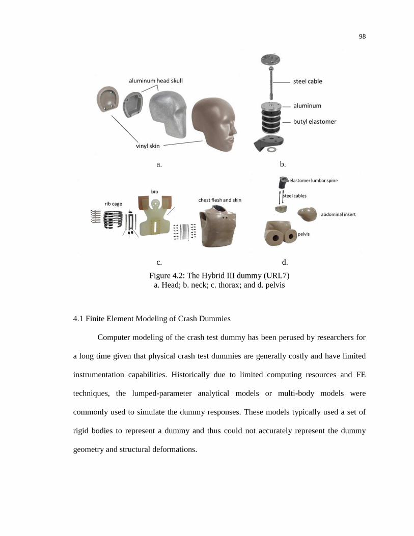
98
a. b.
c. d.
Figure 4.2: The Hybrid III dummy (URL7)
a. Head; b. neck; c. thorax; and d. pelvis
4.1 Finite Element Modeling of Crash Dummies
Computer modeling of the crash test dummy has been perused by researchers for
a long time given that physical crash test dummies are generally costly and have limited
instrumentation capabilities. Historically due to limited computing resources and FE
techniques, the lumped-parameter analytical models or multi-body models were
commonly used to simulate the dummy responses. These models typically used a set of
rigid bodies to represent a dummy and thus could not accurately represent the dummy
geometry and structural deformations.
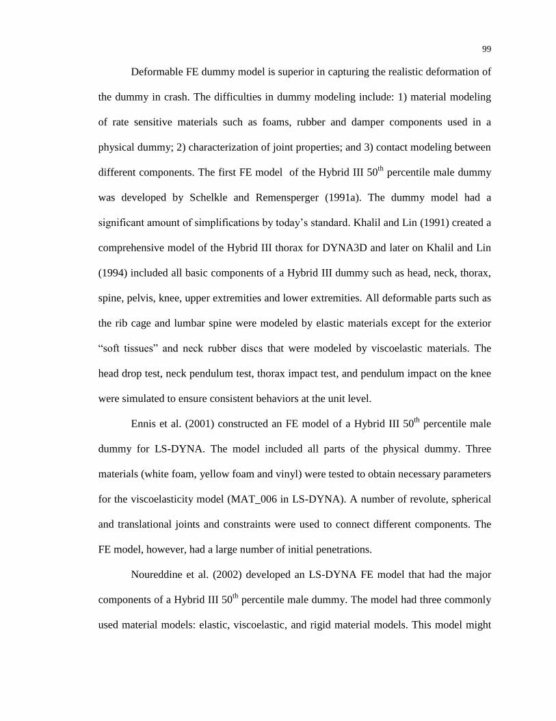
99
Deformable FE dummy model is superior in capturing the realistic deformation of
the dummy in crash. The difficulties in dummy modeling include: 1) material modeling
of rate sensitive materials such as foams, rubber and damper components used in a
physical dummy; 2) characterization of joint properties; and 3) contact modeling between
different components. The first FE model of the Hybrid III 50th
percentile male dummy
was developed by Schelkle and Remensperger (1991a). The dummy model had a
significant amount of simplifications by today’s standard. Khalil and Lin (1991) created a
comprehensive model of the Hybrid III thorax for DYNA3D and later on Khalil and Lin
(1994) included all basic components of a Hybrid III dummy such as head, neck, thorax,
spine, pelvis, knee, upper extremities and lower extremities. All deformable parts such as
the rib cage and lumbar spine were modeled by elastic materials except for the exterior
“soft tissues” and neck rubber discs that were modeled by viscoelastic materials. The
head drop test, neck pendulum test, thorax impact test, and pendulum impact on the knee
were simulated to ensure consistent behaviors at the unit level.
Ennis et al. (2001) constructed an FE model of a Hybrid III 50th
percentile male
dummy for LS-DYNA. The model included all parts of the physical dummy. Three
materials (white foam, yellow foam and vinyl) were tested to obtain necessary parameters
for the viscoelasticity model (MAT_006 in LS-DYNA). A number of revolute, spherical
and translational joints and constraints were used to connect different components. The
FE model, however, had a large number of initial penetrations.
Noureddine et al. (2002) developed an LS-DYNA FE model that had the major
components of a Hybrid III 50th
percentile male dummy. The model had three commonly
used material models: elastic, viscoelastic, and rigid material models. This model might
100
not be sufficient in predicting the femur’s response due to the used of simplified material
models. Krone and Schuster (2006) investigated the importance of including material
anisotropy in the FE model of a human femur. In their study of the anterior-posterior
bending and external-internal rotation, the femur was modeled using four material models:
linear orthotropic, linear transversely isotropic, linear isotropic and non-linear isotropic.
While the force-deflection response of the femur in anterior-posterior bending could be
sufficiently described by isotropic material models, the response of the femur in external-
internal rotation could be better predicted by the orthotropic material models.
Mohan et al. ((2007); (2009b); (2010)) presented the continuous efforts on
developing a LS-DYNA FE model of the Hybrid III 50th
percentile male dummy. The FE
model had more elements and nodes than the aforementioned dummy models. Elastic
material was used for the skeleton, the viscoelastic material model (MAT_006) was used
for the polyvinyl skin, the simple rubber model (MAT_007) was used for the rubber parts
(e.g. flesh), and the viscous foam model (MAT_062) was used for the foam parts (e.g.
pelvis insert). The wire rope used in the neck and lumbar spine was modeled by the
Belytschko-Schwer resultant beam elements with a uniform cross-section.
More recently, Yi et al. (2011) proposed an FE model of a Hybrid III 5th
percentile female dummy. In the material identification process, they used a successive
response surface method to determine the material parameters that would minimize the
differences between the test data and the simulation results.
The main difficulty in dummy modeling lies in material characterization,
particularly for the parts made of foams and rubbers. Another source of difficulty is the
modeling of some complicated components such as the neck. Accurate modeling of the
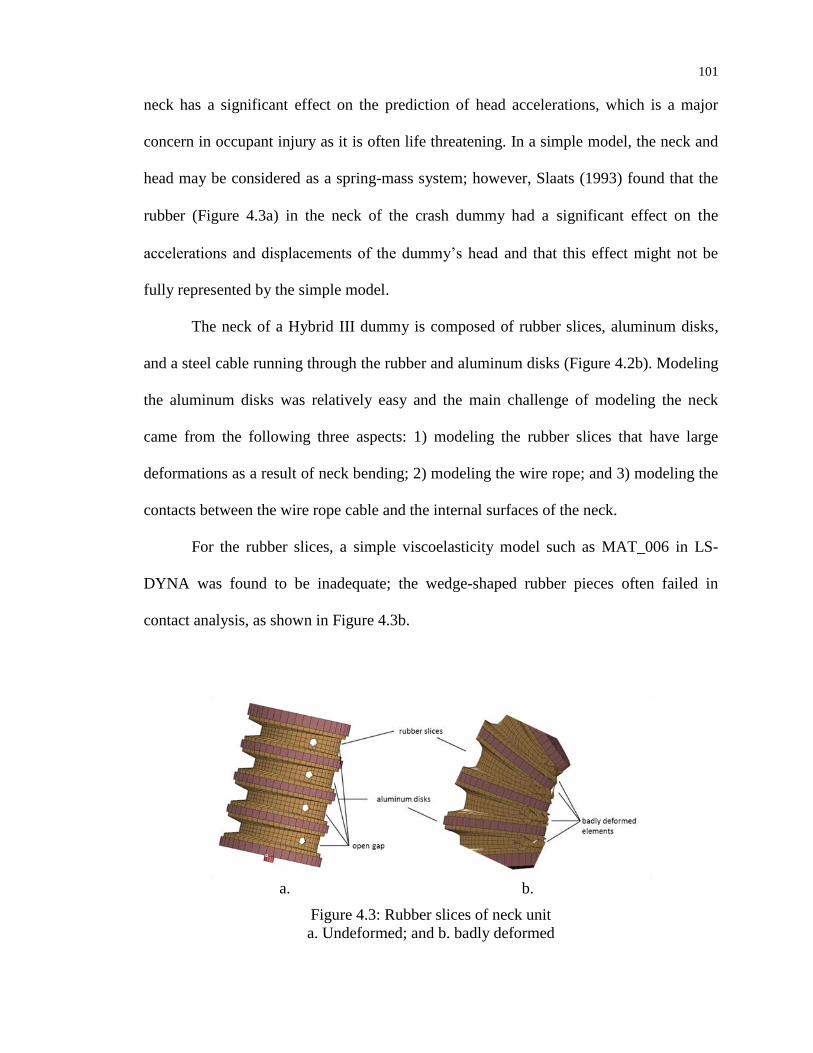
101
neck has a significant effect on the prediction of head accelerations, which is a major
concern in occupant injury as it is often life threatening. In a simple model, the neck and
head may be considered as a spring-mass system; however, Slaats (1993) found that the
rubber (Figure 4.3a) in the neck of the crash dummy had a significant effect on the
accelerations and displacements of the dummy’s head and that this effect might not be
fully represented by the simple model.
The neck of a Hybrid III dummy is composed of rubber slices, aluminum disks,
and a steel cable running through the rubber and aluminum disks (Figure 4.2b). Modeling
the aluminum disks was relatively easy and the main challenge of modeling the neck
came from the following three aspects: 1) modeling the rubber slices that have large
deformations as a result of neck bending; 2) modeling the wire rope; and 3) modeling the
contacts between the wire rope cable and the internal surfaces of the neck.
For the rubber slices, a simple viscoelasticity model such as MAT_006 in LS-
DYNA was found to be inadequate; the wedge-shaped rubber pieces often failed in
contact analysis, as shown in Figure 4.3b.
a. b.
Figure 4.3: Rubber slices of neck unit
a. Undeformed; and b. badly deformed

102
The wire rope in the neck is made of a 7x19 cable with a diameter of 7.9 mm
(5/16 inch) and a nominal cross-sectional area of 49 mm2 (0.0767 inch
2) (Figure 4.4). As
seen from Figure 4.4, the cross-section of the wire rope is not a fully circular area and
thus it is appropriate to use the “metallic cross-sectional area” that only accounts for the
total areas of the individual wires without including the gaps. The wire rope in the
dummy’s neck has a “metallic cross-sectional area” of 30 mm2
(0.0465 inch2).
Figure 4.4: A 7x19 wire rope and its cross-section (URL8)
The simplest way to model a wire rope is to use beam elements with the “metallic
cross-sectional area” and linear elastic material model. Material properties are then
calibrated to obtain the true stiffness under tensile, bending and torsional loading
conditions. In the work by Mohan et al. (2007), the wire rope was modeled by the
Belytshcko-Schwer resultant beam elements with a diameter of 6.18 mm, Young’s
modulus of 96 GPa, and density of 7.89106 kg/m
3. The difficulty with an elastic
material model is that the different behaviors of the steel cable in tension and
compression and in non-linear bending cannot be captured (Franz and Graf 2000).
Additionally, the elastic material model has no damping mechanism that exists in the
wired rope (energy loss due to friction in relative fiber movements). Furthermore,
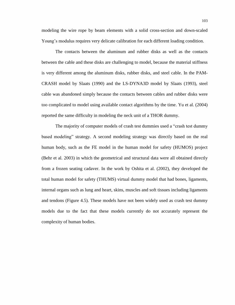
103
modeling the wire rope by beam elements with a solid cross-section and down-scaled
Young’s modulus requires very delicate calibration for each different loading condition.
The contacts between the aluminum and rubber disks as well as the contacts
between the cable and these disks are challenging to model, because the material stiffness
is very different among the aluminum disks, rubber disks, and steel cable. In the PAM-
CRASH model by Slaats (1990) and the LS-DYNA3D model by Slaats (1993), steel
cable was abandoned simply because the contacts between cables and rubber disks were
too complicated to model using available contact algorithms by the time. Yu et al. (2004)
reported the same difficulty in modeling the neck unit of a THOR dummy.
The majority of computer models of crash test dummies used a “crash test dummy
based modeling” strategy. A second modeling strategy was directly based on the real
human body, such as the FE model in the human model for safety (HUMOS) project
(Behr et al. 2003) in which the geometrical and structural data were all obtained directly
from a frozen seating cadaver. In the work by Oshita et al. (2002), they developed the
total human model for safety (THUMS) virtual dummy model that had bones, ligaments,
internal organs such as lung and heart, skins, muscles and soft tissues including ligaments
and tendons (Figure 4.5). These models have not been widely used as crash test dummy
models due to the fact that these models currently do not accurately represent the
complexity of human bodies.
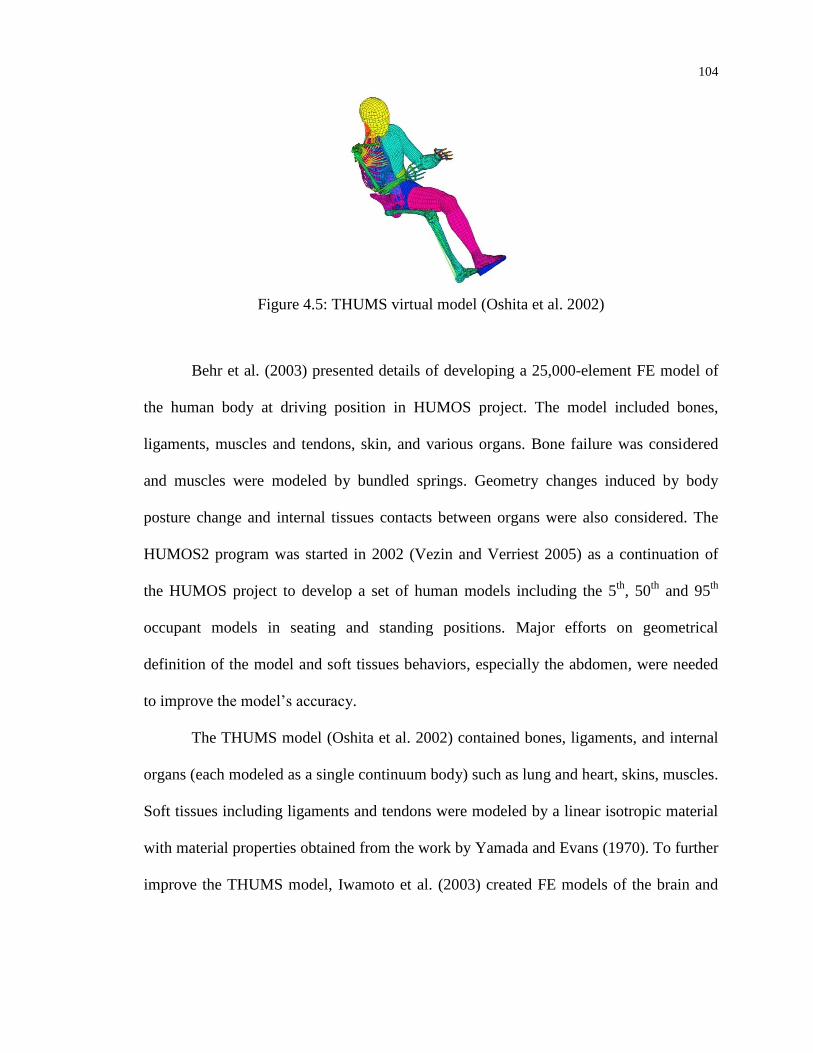
104
Figure 4.5: THUMS virtual model (Oshita et al. 2002)
Behr et al. (2003) presented details of developing a 25,000-element FE model of
the human body at driving position in HUMOS project. The model included bones,
ligaments, muscles and tendons, skin, and various organs. Bone failure was considered
and muscles were modeled by bundled springs. Geometry changes induced by body
posture change and internal tissues contacts between organs were also considered. The
HUMOS2 program was started in 2002 (Vezin and Verriest 2005) as a continuation of
the HUMOS project to develop a set of human models including the 5th
, 50th
and 95th
occupant models in seating and standing positions. Major efforts on geometrical
definition of the model and soft tissues behaviors, especially the abdomen, were needed
to improve the model’s accuracy.
The THUMS model (Oshita et al. 2002) contained bones, ligaments, and internal
organs (each modeled as a single continuum body) such as lung and heart, skins, muscles.
Soft tissues including ligaments and tendons were modeled by a linear isotropic material
with material properties obtained from the work by Yamada and Evans (1970). To further
improve the THUMS model, Iwamoto et al. (2003) created FE models of the brain and

105
individual internal organs including the heart, lung, stomach, liver, spleen, pancreas,
kidney, intestine, aorta, and vena cava.
The THUMS and HUMOS virtual dummy models are highly detailed universal
human models. Theoretically, they can be used in any type of crash scenarios since they
are computational models of a full human body including lifelike details of the flesh,
bones, ligaments, blood vessels, and organs. They are relatively new dummy models and
have not gain popularity due to lack of sufficient validation, government regulations, and
a number of other reasons. To this end, direct modeling a crash test dummy hardware is
still the dominant approach for safety studies. It should be noted that each of the crash
test dummies and the corresponding dummy models is developed for a particular crash
scenario such as frontal, side, or rear impacts; they cannot be interchangeably used in
different impact scenarios. For example, the Hybrid III 50th
percentile male FID should
generally be used in frontal crashes and is not suitable for side impact. In reality oblique
impact such as roadside barrier crash is more often than a perfect frontal impact or side
impact. A crash test dummy combing the features of an FID and a SID would be ideal but
is currently unavailable due to the difficulties in creating reliable and repeatable dummy
hardware. Due to restrictions and limitations of the FID and SID dummies, oblique
impacts, as seen in most roadside barrier crashes, cannot be well addressed by either the
FID or SID alone. In fact, there are no restrictions or regulations that forbid the usage of
frontal impact dummies in roadside barrier crashes. On the contrary, adopting a Hybrid
III dummy in median barrier crash testing is encouraged by MASH. A few testing
agencies have started using Hybrid III dummies in roadside barrier crash tests.
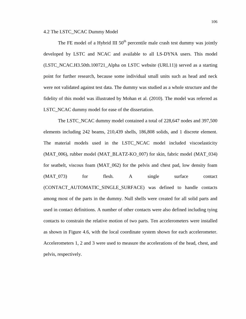
106
4.2 The LSTC_NCAC Dummy Model
The FE model of a Hybrid III 50th
percentile male crash test dummy was jointly
developed by LSTC and NCAC and available to all LS-DYNA users. This model
(LSTC_NCAC.H3.50th.100721_Alpha on LSTC website (URL11)) served as a starting
point for further research, because some individual small units such as head and neck
were not validated against test data. The dummy was studied as a whole structure and the
fidelity of this model was illustrated by Mohan et al. (2010). The model was referred as
LSTC_NCAC dummy model for ease of the dissertation.
The LSTC_NCAC dummy model contained a total of 228,647 nodes and 397,500
elements including 242 beams, 210,439 shells, 186,808 solids, and 1 discrete element.
The material models used in the LSTC_NCAC model included viscoelasticity
(MAT_006), rubber model (MAT_BLATZ-KO_007) for skin, fabric model (MAT_034)
for seatbelt, viscous foam (MAT_062) for the pelvis and chest pad, low density foam
(MAT_073) for flesh. A single surface contact
(CONTACT_AUTOMATIC_SINGLE_SURFACE) was defined to handle contacts
among most of the parts in the dummy. Null shells were created for all solid parts and
used in contact definitions. A number of other contacts were also defined including tying
contacts to constrain the relative motion of two parts. Ten accelerometers were installed
as shown in Figure 4.6, with the local coordinate system shown for each accelerometer.
Accelerometers 1, 2 and 3 were used to measure the accelerations of the head, chest, and
pelvis, respectively.
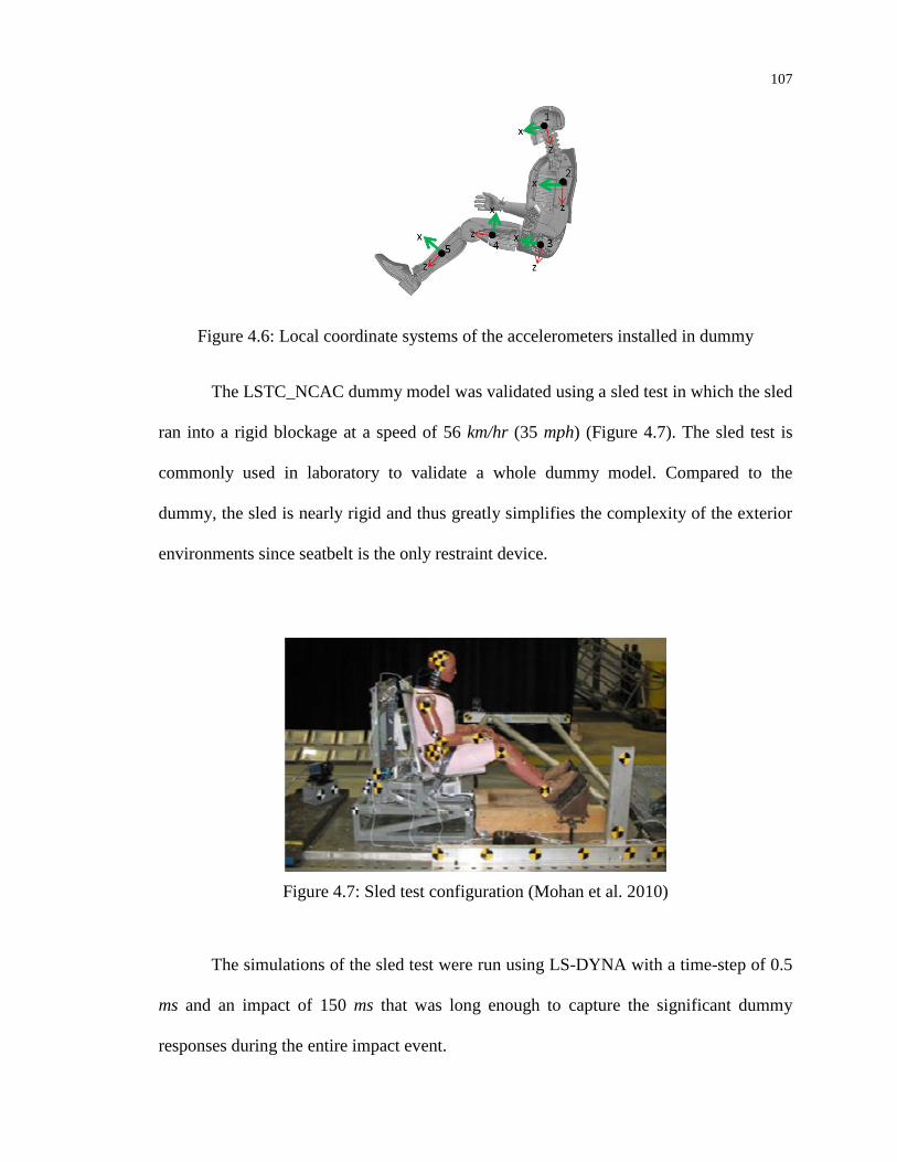
107
Figure 4.6: Local coordinate systems of the accelerometers installed in dummy
The LSTC_NCAC dummy model was validated using a sled test in which the sled
ran into a rigid blockage at a speed of 56 km/hr (35 mph) (Figure 4.7). The sled test is
commonly used in laboratory to validate a whole dummy model. Compared to the
dummy, the sled is nearly rigid and thus greatly simplifies the complexity of the exterior
environments since seatbelt is the only restraint device.
Figure 4.7: Sled test configuration (Mohan et al. 2010)
The simulations of the sled test were run using LS-DYNA with a time-step of 0.5
ms and an impact of 150 ms that was long enough to capture the significant dummy
responses during the entire impact event.
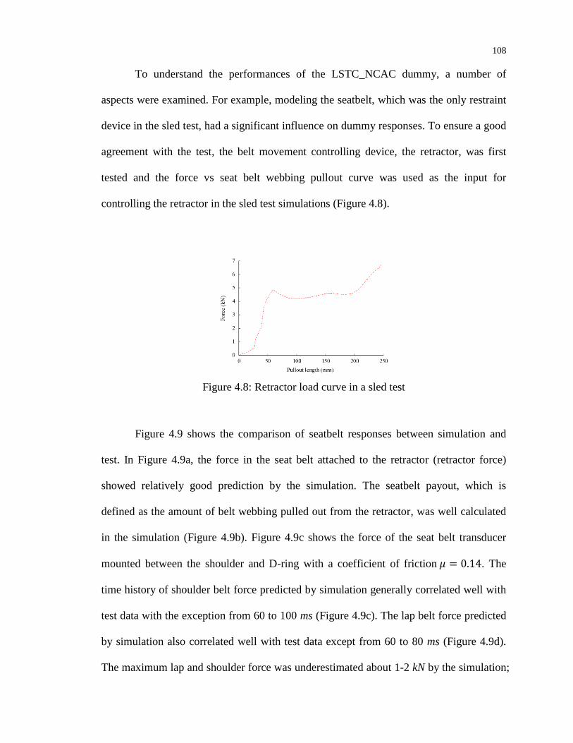
108
To understand the performances of the LSTC_NCAC dummy, a number of
aspects were examined. For example, modeling the seatbelt, which was the only restraint
device in the sled test, had a significant influence on dummy responses. To ensure a good
agreement with the test, the belt movement controlling device, the retractor, was first
tested and the force vs seat belt webbing pullout curve was used as the input for
controlling the retractor in the sled test simulations (Figure 4.8).
Figure 4.8: Retractor load curve in a sled test
Figure 4.9 shows the comparison of seatbelt responses between simulation and
test. In Figure 4.9a, the force in the seat belt attached to the retractor (retractor force)
showed relatively good prediction by the simulation. The seatbelt payout, which is
defined as the amount of belt webbing pulled out from the retractor, was well calculated
in the simulation (Figure 4.9b). Figure 4.9c shows the force of the seat belt transducer
mounted between the shoulder and D-ring with a coefficient of friction . The
time history of shoulder belt force predicted by simulation generally correlated well with
test data with the exception from 60 to 100 ms (Figure 4.9c). The lap belt force predicted
by simulation also correlated well with test data except from 60 to 80 ms (Figure 4.9d).
The maximum lap and shoulder force was underestimated about 1-2 kN by the simulation;

109
this was the largest source of discrepancy between simulation results and test data. The
lap belt force reached its peak earlier in the simulation than in the test. While the retractor
force was simulated quite well, the shoulder belt force was off by a larger amount. The
significance of this mismatch was that if the shoulder belt force were brought up to match
the test data, it might increase the chest deflection correspondingly.
a. b.
c. d.
Figure 4.9: Seat belt responses by LSTC_NCAC model ( )
a. Retractor force; b. belt payout; c. shoulder belt force; and d. lap belt force
The kinematic responses of the dummy should agree well with the test to ensure
consistent dynamics. The snapshots of a sled test were used to compare with simulation
results at three different time instances (Figure 4.10). The simulated dummy posture at
100 ms was very close to that in the test. Additionally, a few other observations could be

110
made: 1) the motions of hands and arms were different between simulation results and
test data; 2) the gap between the head and knee in the simulation was not the same as in
the test; 3) the dummy feet lost partial contact with the resting plate in the test while the
dummy feet remained full contact in the simulation at 150 ms; and 4) the upper body of
the dummy bended/leaned forward more in the test than in simulation. Considering that
the LSTC_NCAC model underestimated shoulder belt force (Figure 4.9c), it implied that
the upper body of the FE dummy model was stiffer than the real dummy, which resulted
in a smaller forward bending motion even with a less severe belt restraint than the test.
Possible reasons included that penetrations between parts inside the upper body locked
their relative motions to some extent.
0 ms 100 ms 150 ms
Figure 4.10: Comparison of simulated dummy profile by LSTC_NCAC model to test
data (Mohan et al. 2010)
111
Accelerations experienced by the head, chest and pelvis were important
information to assess the potential injury especially to the head. Acceleration data of both
tests and simulations were filtered using standard filters given in Table 4.1.
Table 4.1: Filters for different data channels
Data Channel Filter Class
Head Accelerometer CFC_1000
Chest Accelerometer CFC_180
Pelvis Accelerometer CFC_1000
Femur Force CFC_1000
Chest Deflection CFC_600
Seat Belt Force CFC_60
The major differences in the time history of dummy accelerations between
simulation results and test data, as shown in Figure 4.11, are: 1) the peak resultant
acceleration on the head was over-predicted by 10 g in the simulation (Figure 4.11a); 2)
the first peak resultant acceleration on the chest was underestimated by 15 g in the
simulation and the second peak acceleration was completely missed in the simulation
(Figure 4.11b); and 3) the peak acceleration on the pelvis was 5 ms earlier in the
simulation than in the test (Figure 4.11c).
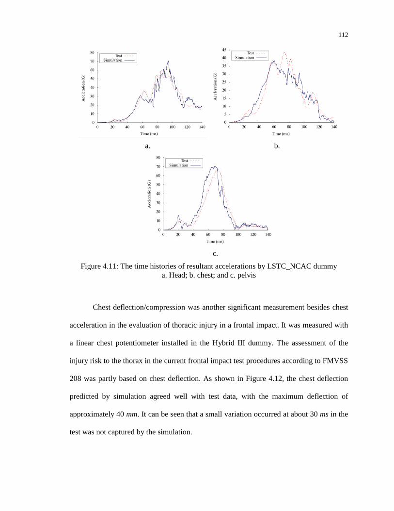
112
a. b.
c.
Figure 4.11: The time histories of resultant accelerations by LSTC_NCAC dummy
a. Head; b. chest; and c. pelvis
Chest deflection/compression was another significant measurement besides chest
acceleration in the evaluation of thoracic injury in a frontal impact. It was measured with
a linear chest potentiometer installed in the Hybrid III dummy. The assessment of the
injury risk to the thorax in the current frontal impact test procedures according to FMVSS
208 was partly based on chest deflection. As shown in Figure 4.12, the chest deflection
predicted by simulation agreed well with test data, with the maximum deflection of
approximately 40 mm. It can be seen that a small variation occurred at about 30 ms in the
test was not captured by the simulation.
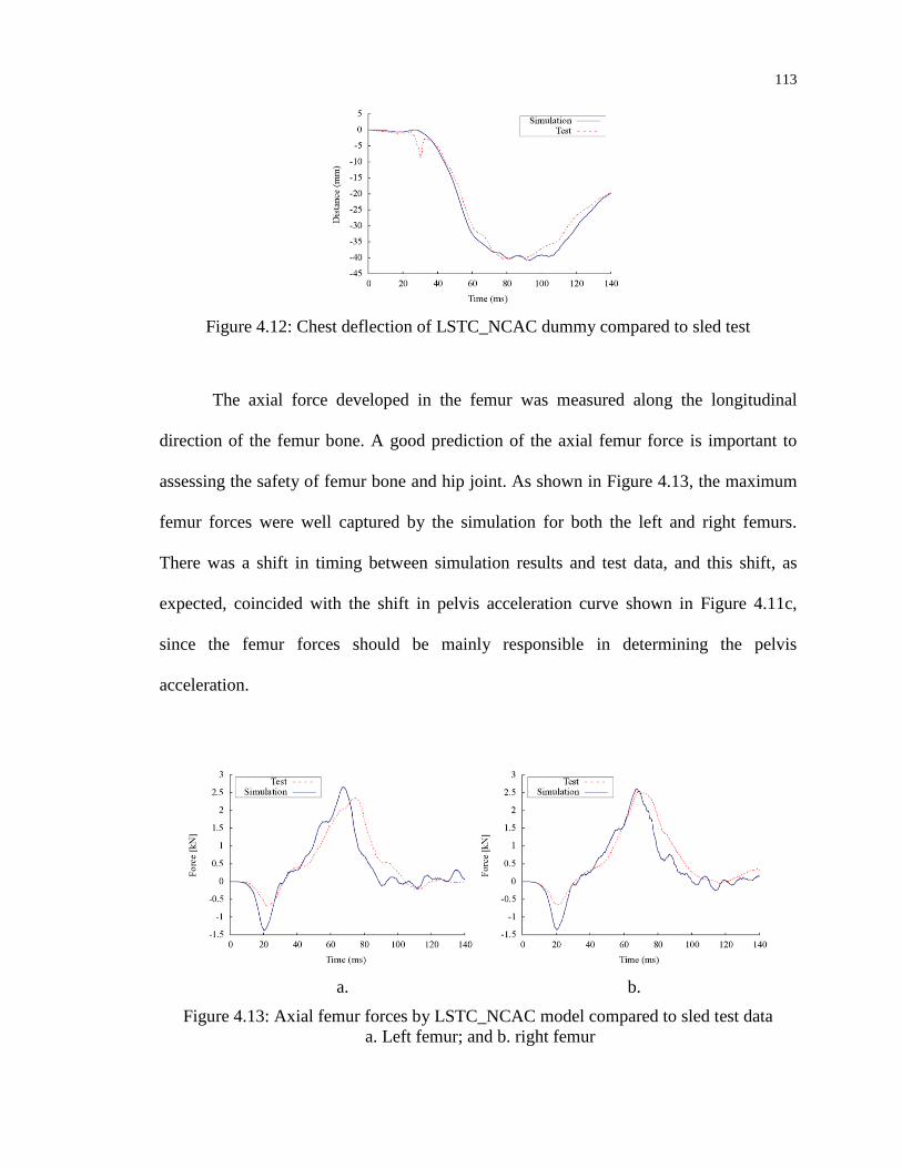
113
Figure 4.12: Chest deflection of LSTC_NCAC dummy compared to sled test
The axial force developed in the femur was measured along the longitudinal
direction of the femur bone. A good prediction of the axial femur force is important to
assessing the safety of femur bone and hip joint. As shown in Figure 4.13, the maximum
femur forces were well captured by the simulation for both the left and right femurs.
There was a shift in timing between simulation results and test data, and this shift, as
expected, coincided with the shift in pelvis acceleration curve shown in Figure 4.11c,
since the femur forces should be mainly responsible in determining the pelvis
acceleration.
a. b.
Figure 4.13: Axial femur forces by LSTC_NCAC model compared to sled test data
a. Left femur; and b. right femur
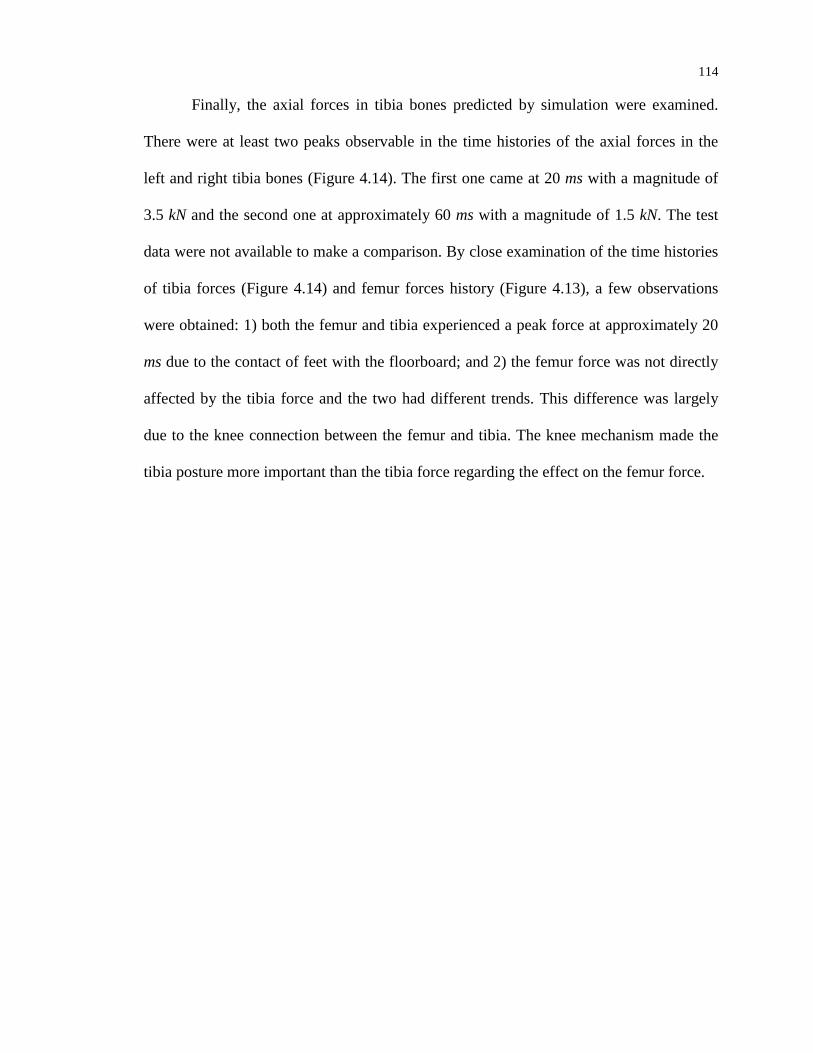
114
Finally, the axial forces in tibia bones predicted by simulation were examined.
There were at least two peaks observable in the time histories of the axial forces in the
left and right tibia bones (Figure 4.14). The first one came at 20 ms with a magnitude of
3.5 kN and the second one at approximately 60 ms with a magnitude of 1.5 kN. The test
data were not available to make a comparison. By close examination of the time histories
of tibia forces (Figure 4.14) and femur forces history (Figure 4.13), a few observations
were obtained: 1) both the femur and tibia experienced a peak force at approximately 20
ms due to the contact of feet with the floorboard; and 2) the femur force was not directly
affected by the tibia force and the two had different trends. This difference was largely
due to the knee connection between the femur and tibia. The knee mechanism made the
tibia posture more important than the tibia force regarding the effect on the femur force.
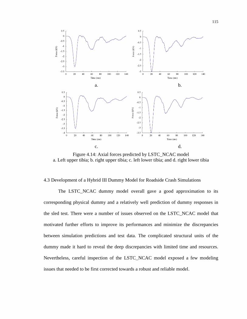
115
a. b.
c. d.
Figure 4.14: Axial forces predicted by LSTC_NCAC model
a. Left upper tibia; b. right upper tibia; c. left lower tibia; and d. right lower tibia
4.3 Development of a Hybrid III Dummy Model for Roadside Crash Simulations
The LSTC_NCAC dummy model overall gave a good approximation to its
corresponding physical dummy and a relatively well prediction of dummy responses in
the sled test. There were a number of issues observed on the LSTC_NCAC model that
motivated further efforts to improve its performances and minimize the discrepancies
between simulation predictions and test data. The complicated structural units of the
dummy made it hard to reveal the deep discrepancies with limited time and resources.
Nevertheless, careful inspection of the LSTC_NCAC model exposed a few modeling
issues that needed to be first corrected towards a robust and reliable model.

116
One of the major issues of the LSTC_NCAC model was the existence of a large
amount of initial penetrations. Initial penetrations were almost guaranteed to be present
during the meshing and assembling phase due to the geometric complexity and presence
of many soft foam pads in the dummy hardware (Ennis et al. 2001). Initial penetrations
need to be eliminated once the whole dummy model is assembled from individual
components, because these penetrations not only cause numerical instability of the
simulations, but also produce incorrect dummy responses and thus low-fidelity of the
simulation results. Contact penetrations often lead to badly deformed elements and
simulation was often terminated as a result of which. The large amount of penetrations in
LSTC_NCAC dummy model led to violation of energy conservation as can be seen in
Figure 4.15. This was because, as pointed out in section 3.1.1, existence of contact
penetrations leads to negative contact energy and thus a loss of total energy.
Figure 4.15: Energy ratio by the LSTC_NCAC model in sled test
Initial penetrations may prevent relative motion between contacting parts. For
example, there were initial penetrations between the feet and floorboard in the
LSTC_NCAC dummy model (Figure 4.16). These penetrations persisted throughout the

117
entire simulation course and prevented the feet from moving away from the sled plate, as
seen in the sled test.
Figure 4.16: Side view of feet motion relative to the floorboard by LSTC_NCAC model
Penetrations could also be a result of failed contact handling during the simulation
even without initial penetrations. For example, the contact between cables and rubber
disks in the neck unit failed during simulation and resulted in badly deformed elements
(Figure 4.17) in later stages of the simulation using the LSTC_NCAC model.
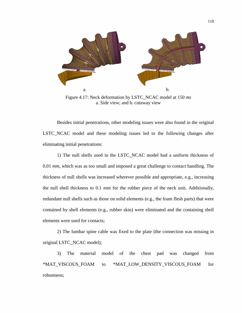
118
a. b.
Figure 4.17: Neck deformation by LSTC_NCAC model at 150 ms
a. Side view; and b. cutaway view
Besides initial penetrations, other modeling issues were also found in the original
LSTC_NCAC model and these modeling issues led to the following changes after
eliminating initial penetrations:
1) The null shells used in the LSTC_NCAC model had a uniform thickness of
0.01 mm, which was as too small and imposed a great challenge to contact handling. The
thickness of null shells was increased wherever possible and appropriate, e.g., increasing
the null shell thickness to 0.1 mm for the rubber piece of the neck unit. Additionally,
redundant null shells such as those on solid elements (e.g., the foam flesh parts) that were
contained by shell elements (e.g., rubber skin) were eliminated and the containing shell
elements were used for contacts;
2) The lumbar spine cable was fixed to the plate (the connection was missing in
original LSTC_NCAC model);
3) The material model of the chest pad was changed from
*MAT_VISCOUS_FOAM to *MAT_LOW_DENSITY_VISCOUS_FOAM for
robustness;

119
4) The shoulder pad was tied to the bib assembly plate using tying contact instead
of spot-welds between these two parts. Spot-welds often resulted in bad deformed
elements since they imposed point loads to the foam pad;
5) The steel cable in the neck and lumbar spine was modeled using the
INITIAL_AXIAL_FORCE_BEAM, replacing the original INITIAL_STRESS_BEAM
element for better imposing the initial stress;
6) The CONTACT_AUTOMATIC_TIED_NODES_TO_SURFACE caused
significant geometry change and elements skew; thus it was replaced by
CONTACT_AUTOMATIC_TIED_NODES_TO_SURFACE_OFFSET;
7) A tying contact was defined to tie the pelvis insert foam to the pelvis inner
cover;
8) The element-free Galerkin formulation was used on solid elements of rubber
disks of the neck unit to improve the performance of the elements under large and
irregular deformation;
9) Contact algorithm between the seatbelt and dummy was switched to surface-to-
surface contact to handle edge-to-edge contacts; and
10) The friction coefficient between the D-ring and seatbelt was changed to 0.25
from 0.14 in the original LSTC_NCAC model to ensure a consistent belt force between
the simulation and test.
4.4 Validation of the Revised Dummy Model: ISOL Dummy Model
With the modifications and improvements to the LSTC_NCAC model, the new
dummy model, designated as the ISOL dummy model, was shown to have improved
numerical stability and robustness. To ensure the ISOL dummy model had good

120
agreement with test data, the new dummy FE model was validated using a sled test, a
frontal impact test, and a 40% offset impact test.
4.4.1 Sled Test
The simulation results of the sled test using ISOL dummy model showed the first
improvements from the seatbelt responses. The D-Ring (Figure 4.18a), which was the
only device between the shoulder belt and the retractor, was modeled by a slip-ring
element in LS-DYNA (Figure 4.18c). This element played an important role in relating
the shoulder belt force to retractor force. By varying the friction coefficient between
seatbelt and D-ring, better agreements could be reached with test data (Figure 4.19).
a. b. c.
Figure 4.18: Models of D-ring
a. A D-ring physical model (Pedrazzi et al. 2001); b. a full 3-D FE model (Dubois et al.
2006); and c. a simplified slipring model by LS-DYNA

121
a. b.
c. d.
Figure 4.19: Seat belt responses by ISOL model a. Retractor force; b. belt payout; c. shoulder belt force; and d. lap belt force
As can be seen in Figure 4.19, there was a reasonably good match between
simulation results and test data on both the shoulder belt force and retractor force. In the
simulation results, a plateau region in the retractor force was seen from 90 to 110 ms
where the peak force seen in test data was missed. In the same time period, a peak
shoulder belt force was reached around 90 ms, followed by an abrupt decrease that
matched the abrupt decrease in retractor force. The mismatch between simulation results
on retractor and shoulder belt forces implied a potential inherent modeling deficiency in
the slip ring element, which was a single dimensionless node with user defined friction.
The slip ring element was not able to capture the full behavior of a 3-d D-ring and the

122
seatbelt webbing interaction (Figure 4.18b). For a full 3-D model and discussions about
D-ring behaviors, refer to (Dubois et al. 2006; Dubois et al. 2011; Dubois et al. 2009;
Pedrazzi et al. 2001).
As a direct and noticeable influence of the improved prediction on shoulder belt
and lap belt forces, the prediction on chest deflection by simulation matched well to test
data, as seen in Figure 4.20.
Figure 4.20: Chest deflection by ISOL dummy model in a sled test
The dummy postures predicted by simulations at 100 ms and 150 ms matched
well to test data (Figure 4.21), compared to those by the LSTC_NCAC model in Figure
4.10. Despite the mismatch on hand and arms motions at 150 ms, the head position and
the upper body postures were consistent to those seen in the test.

123
0 ms 100 ms 150 ms
Figure 4.21: Comparison of simulated dummy profile by ISOL model to sled test
Besides the small mismatches at 80 and 110 ms as shown in Figure 4.22a, the
head resultant acceleration predicted by simulation was in line with test data with the
peak value well captured. The chest resultant acceleration by simulation had 10 ms delay
on the second peak comparing to test data (Figure 4.22b), and the pelvis resultant
acceleration was consistent with test data (Figure 4.22c).
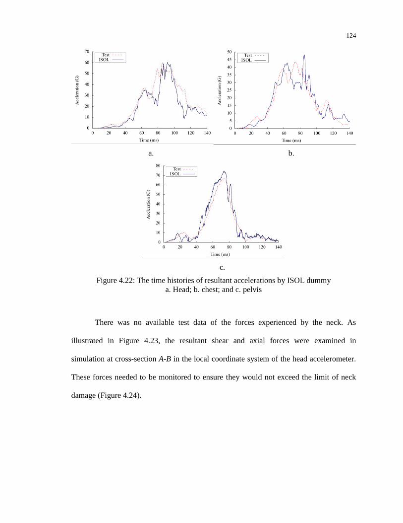
124
a. b.
c.
Figure 4.22: The time histories of resultant accelerations by ISOL dummy
a. Head; b. chest; and c. pelvis
There was no available test data of the forces experienced by the neck. As
illustrated in Figure 4.23, the resultant shear and axial forces were examined in
simulation at cross-section A-B in the local coordinate system of the head accelerometer.
These forces needed to be monitored to ensure they would not exceed the limit of neck
damage (Figure 4.24).
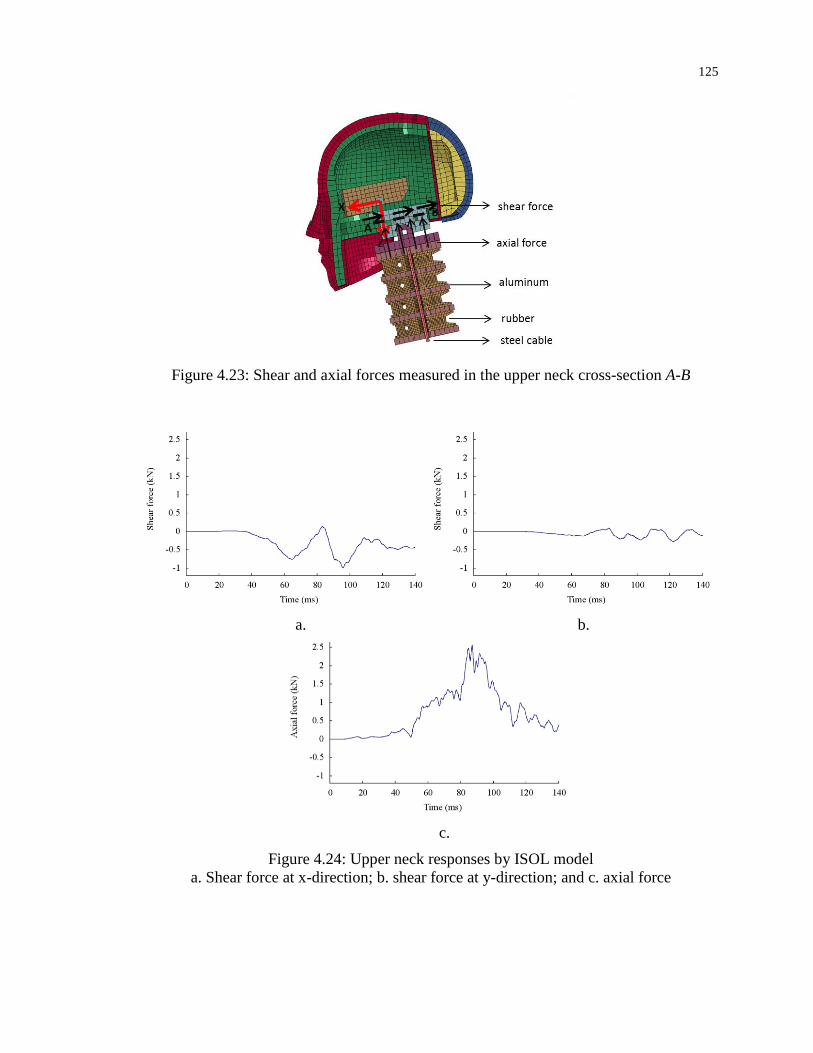
125
Figure 4.23: Shear and axial forces measured in the upper neck cross-section A-B
a. b.
c.
Figure 4.24: Upper neck responses by ISOL model
a. Shear force at x-direction; b. shear force at y-direction; and c. axial force
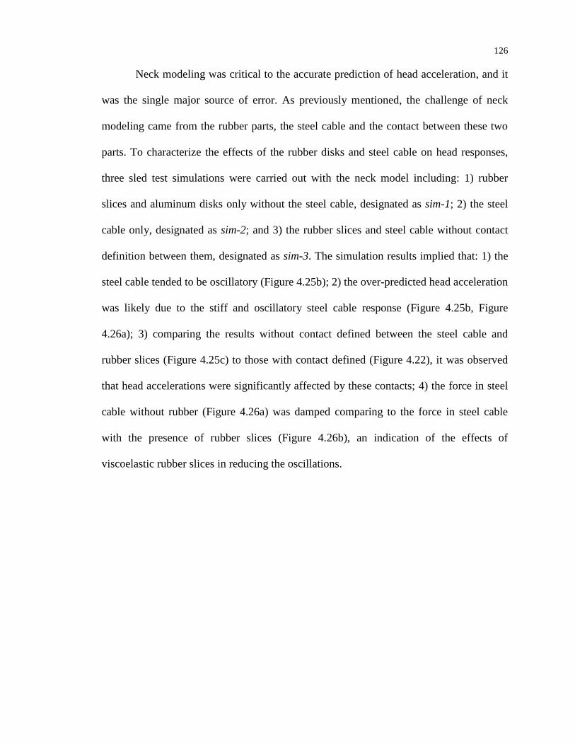
126
Neck modeling was critical to the accurate prediction of head acceleration, and it
was the single major source of error. As previously mentioned, the challenge of neck
modeling came from the rubber parts, the steel cable and the contact between these two
parts. To characterize the effects of the rubber disks and steel cable on head responses,
three sled test simulations were carried out with the neck model including: 1) rubber
slices and aluminum disks only without the steel cable, designated as sim-1; 2) the steel
cable only, designated as sim-2; and 3) the rubber slices and steel cable without contact
definition between them, designated as sim-3. The simulation results implied that: 1) the
steel cable tended to be oscillatory (Figure 4.25b); 2) the over-predicted head acceleration
was likely due to the stiff and oscillatory steel cable response (Figure 4.25b, Figure
4.26a); 3) comparing the results without contact defined between the steel cable and
rubber slices (Figure 4.25c) to those with contact defined (Figure 4.22), it was observed
that head accelerations were significantly affected by these contacts; 4) the force in steel
cable without rubber (Figure 4.26a) was damped comparing to the force in steel cable
with the presence of rubber slices (Figure 4.26b), an indication of the effects of
viscoelastic rubber slices in reducing the oscillations.

127
a. b.
c.
Figure 4.25: The time history of resultant acceleration of the head
a. sim-1; b. sim-2; and c. sim-3
a. b.
Figure 4.26: Axial force of steel cable in the neck unit
a. sim-2; and b. sim-3
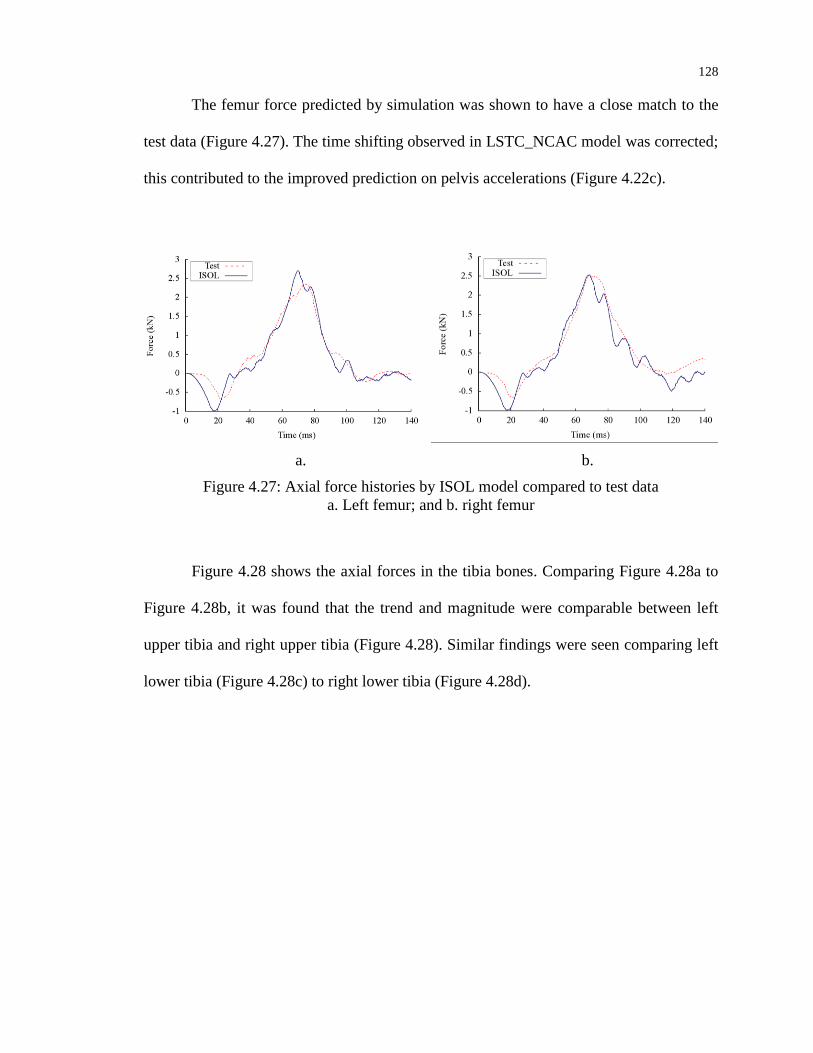
128
The femur force predicted by simulation was shown to have a close match to the
test data (Figure 4.27). The time shifting observed in LSTC_NCAC model was corrected;
this contributed to the improved prediction on pelvis accelerations (Figure 4.22c).
a. b.
Figure 4.27: Axial force histories by ISOL model compared to test data
a. Left femur; and b. right femur
Figure 4.28 shows the axial forces in the tibia bones. Comparing Figure 4.28a to
Figure 4.28b, it was found that the trend and magnitude were comparable between left
upper tibia and right upper tibia (Figure 4.28). Similar findings were seen comparing left
lower tibia (Figure 4.28c) to right lower tibia (Figure 4.28d).
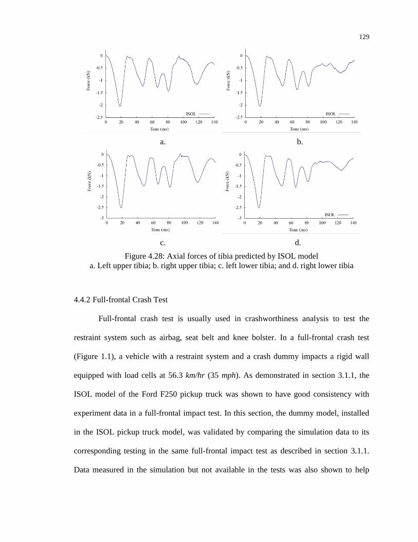
129
a. b.
c. d.
Figure 4.28: Axial forces of tibia predicted by ISOL model
a. Left upper tibia; b. right upper tibia; c. left lower tibia; and d. right lower tibia
4.4.2 Full-frontal Crash Test
Full-frontal crash test is usually used in crashworthiness analysis to test the
restraint system such as airbag, seat belt and knee bolster. In a full-frontal crash test
(Figure 1.1), a vehicle with a restraint system and a crash dummy impacts a rigid wall
equipped with load cells at 56.3 km/hr (35 mph). As demonstrated in section 3.1.1, the
ISOL model of the Ford F250 pickup truck was shown to have good consistency with
experiment data in a full-frontal impact test. In this section, the dummy model, installed
in the ISOL pickup truck model, was validated by comparing the simulation data to its
corresponding testing in the same full-frontal impact test as described in section 3.1.1.
Data measured in the simulation but not available in the tests was also shown to help

130
understand crash behaviors. For example, the force applied to the head from the airbag
was impossible to measure in the test but obtainable in the simulation.
No test data was available to directly characterize the retractor behavior (i.e. force
vs. seatbelt payout curve) in a full-frontal impact was available. The retractor load curve
(Figure 4.29) was obtained by cross plot the shoulder belt force and shoulder D-ring belt
spool. A zero friction coefficient on the shoulder slipring was specified. This
approximately captured the retractor pulling behavior. Apparently the load curve was
very different from that in the sled test as shown in Figure 4.8.
Figure 4.29: Retractor load curve in a frontal impact
Figure 4.30 shows the comparison of simulation results of seat belt forces and belt
spools at D-rings with test data. It can be seen that the shoulder belt force and lap belt
force correlated well with the testing data, while there were discrepancies in belt spools.

131
a. b.
c. d.
Figure 4.30: Seat belt responses by ISOL model in a full-frontal impact
a. Lap belt force; b. belt spool at lap D-ring; c. shoulder belt force; and d. belt spool at
shoulder D-ring
Figure 4.31: Chest compression by ISOL model in a full-frontal impact
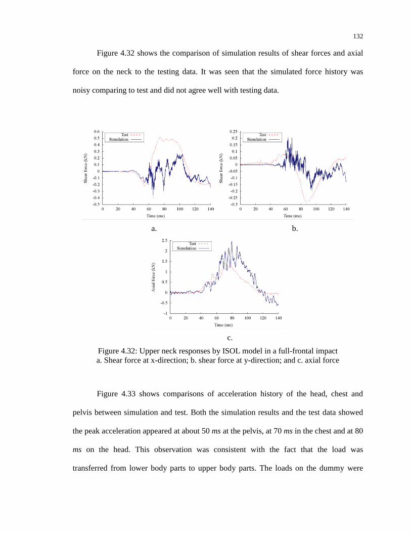
132
Figure 4.32 shows the comparison of simulation results of shear forces and axial
force on the neck to the testing data. It was seen that the simulated force history was
noisy comparing to test and did not agree well with testing data.
a. b.
c.
Figure 4.32: Upper neck responses by ISOL model in a full-frontal impact
a. Shear force at x-direction; b. shear force at y-direction; and c. axial force
Figure 4.33 shows comparisons of acceleration history of the head, chest and
pelvis between simulation and test. Both the simulation results and the test data showed
the peak acceleration appeared at about 50 ms at the pelvis, at 70 ms in the chest and at 80
ms on the head. This observation was consistent with the fact that the load was
transferred from lower body parts to upper body parts. The loads on the dummy were
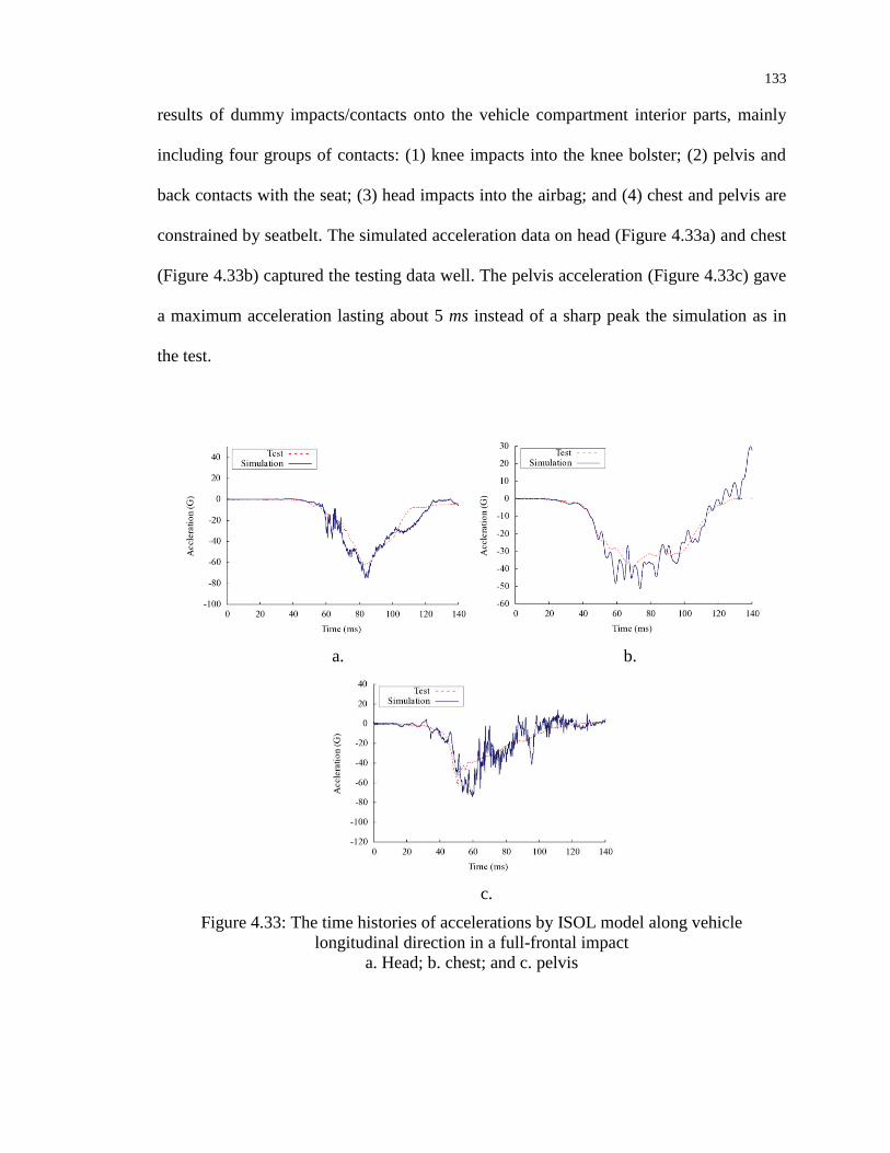
133
results of dummy impacts/contacts onto the vehicle compartment interior parts, mainly
including four groups of contacts: (1) knee impacts into the knee bolster; (2) pelvis and
back contacts with the seat; (3) head impacts into the airbag; and (4) chest and pelvis are
constrained by seatbelt. The simulated acceleration data on head (Figure 4.33a) and chest
(Figure 4.33b) captured the testing data well. The pelvis acceleration (Figure 4.33c) gave
a maximum acceleration lasting about 5 ms instead of a sharp peak the simulation as in
the test.
a. b.
c.
Figure 4.33: The time histories of accelerations by ISOL model along vehicle
longitudinal direction in a full-frontal impact
a. Head; b. chest; and c. pelvis
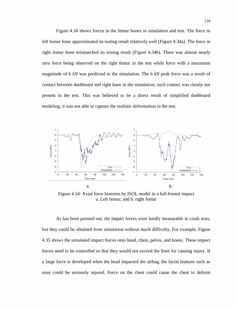
134
Figure 4.34 shows forces in the femur bones in simulation and test. The force in
left femur bone approximated its testing result relatively well (Figure 4.34a). The force in
right femur bone mismatched its testing result (Figure 4.34b). There was almost nearly
zero force being observed on the right femur in the test while force with a maximum
magnitude of 6 kN was predicted in the simulation. The 6 kN peak force was a result of
contact between dashboard and right knee in the simulation; such contact was clearly not
present in the test. This was believed to be a direct result of simplified dashboard
modeling; it was not able to capture the realistic deformation in the test.
a. b.
Figure 4.34: Axial force histories by ISOL model in a full-frontal impact
a. Left femur; and b. right femur
As has been pointed out, the impact forces were hardly measurable in crash tests,
but they could be obtained from simulation without much difficulty. For example, Figure
4.35 shows the simulated impact forces onto head, chest, pelvis, and knees. These impact
forces need to be controlled so that they would not exceed the limit for causing injury. If
a large force is developed when the head impacted the airbag, the facial features such as
nose could be seriously injured. Force on the chest could cause the chest to deform

135
beyond threshold that would break the ribs and damage internal organs such as lungs.
Similarly, the constraints on pelvis by the belt could harmfully compress the internal
organs and cause injuries. Impacts on the knees from the dashboard induce compressive
forces in the femur bones, which are the most significant factors to the safety of femur
bones as well as a reflection of the dashboard in protecting the knees and femurs in a
frontal impact.
a. b.
c. d.
Figure 4.35: Impact forces by ISOL model in a full-frontal impact
a. On head applied from airbag; b. on chest applied from seatbelt;
c. on pelvis applied from seatbelt; and d. on knees applied from dashboard

136
4.4.3 Offset Frontal Crash Test
The configuration of an offset frontal crash test was shown in Figure 1.3. In an
offset frontal impact test, only part of the vehicle’s front hits a deformable barrier made
of aluminum honeycomb. Unlike the full-frontal impact in which the entire vehicle’s
front impacts a rigid wall and the vehicle has no yaw motion, the vehicle developed
noticeable yaw motion in the offset frontal impact as shown in Figure 4.36 and
consequently, the occupant will experience lateral motion and/or acceleration in addition
to longitudinal motions.
a. b. c.
Figure 4.36: Yaw motions of the vehicle in an offset frontal impact
a. 50 ms; b. 100 ms; and c. 150 ms
As shown in section 3.1.2, there were some noticeable differences between the
simulation results for the ISOL pickup truck model and test data. For example, the
vehicle deformation profile was not captured well by the simulation (Figure 4.37).
Damage to the vehicle and compression of the occupant compartment (the roof and the
door) showed apparent differences between simulation and test. This was believed to
have direct consequences on the dummy responses.
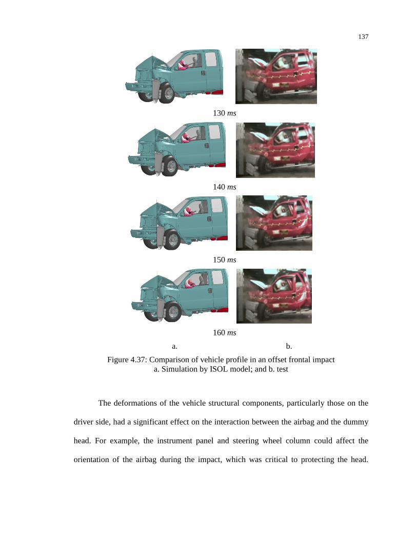
137
130 ms
140 ms
150 ms
160 ms
a. b.
Figure 4.37: Comparison of vehicle profile in an offset frontal impact
a. Simulation by ISOL model; and b. test
The deformations of the vehicle structural components, particularly those on the
driver side, had a significant effect on the interaction between the airbag and the dummy
head. For example, the instrument panel and steering wheel column could affect the
orientation of the airbag during the impact, which was critical to protecting the head.
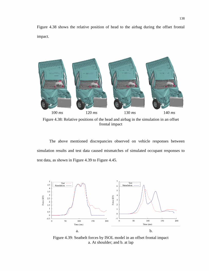
138
Figure 4.38 shows the relative position of head to the airbag during the offset frontal
impact.
100 ms 120 ms 130 ms 140 ms
Figure 4.38: Relative positions of the head and airbag in the simulation in an offset
frontal impact
The above mentioned discrepancies observed on vehicle responses between
simulation results and test data caused mismatches of simulated occupant responses to
test data, as shown in Figure 4.39 to Figure 4.45.
a. b.
Figure 4.39: Seatbelt forces by ISOL model in an offset frontal impact
a. At shoulder; and b. at lap
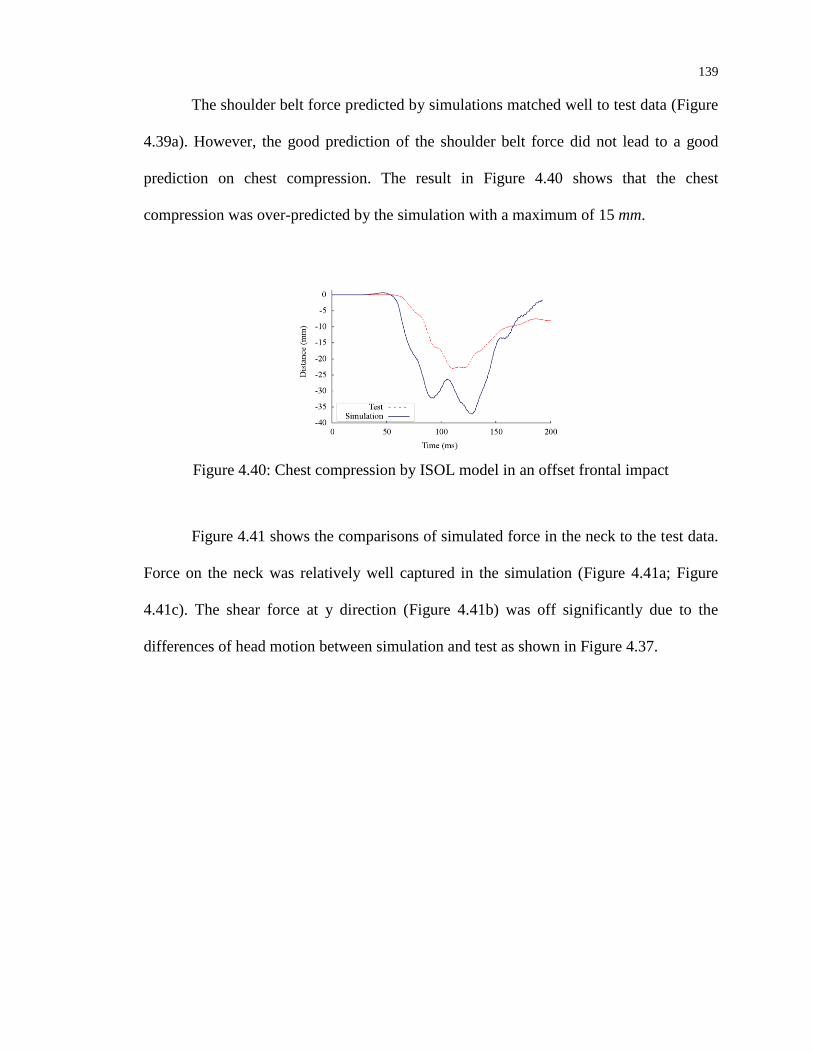
139
The shoulder belt force predicted by simulations matched well to test data (Figure
4.39a). However, the good prediction of the shoulder belt force did not lead to a good
prediction on chest compression. The result in Figure 4.40 shows that the chest
compression was over-predicted by the simulation with a maximum of 15 mm.
Figure 4.40: Chest compression by ISOL model in an offset frontal impact
Figure 4.41 shows the comparisons of simulated force in the neck to the test data.
Force on the neck was relatively well captured in the simulation (Figure 4.41a; Figure
4.41c). The shear force at y direction (Figure 4.41b) was off significantly due to the
differences of head motion between simulation and test as shown in Figure 4.37.
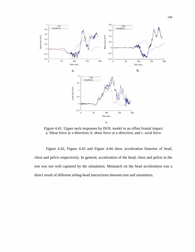
140
a. b.
c.
Figure 4.41: Upper neck responses by ISOL model in an offset frontal impact
a. Shear force at x-direction; b. shear force at y-direction; and c. axial force
Figure 4.42, Figure 4.43 and Figure 4.44 show acceleration histories of head,
chest and pelvis respectively. In general, acceleration of the head, chest and pelvis in the
test was not well captured by the simulation. Mismatch on the head acceleration was a
direct result of different airbag-head interactions between test and simulation.
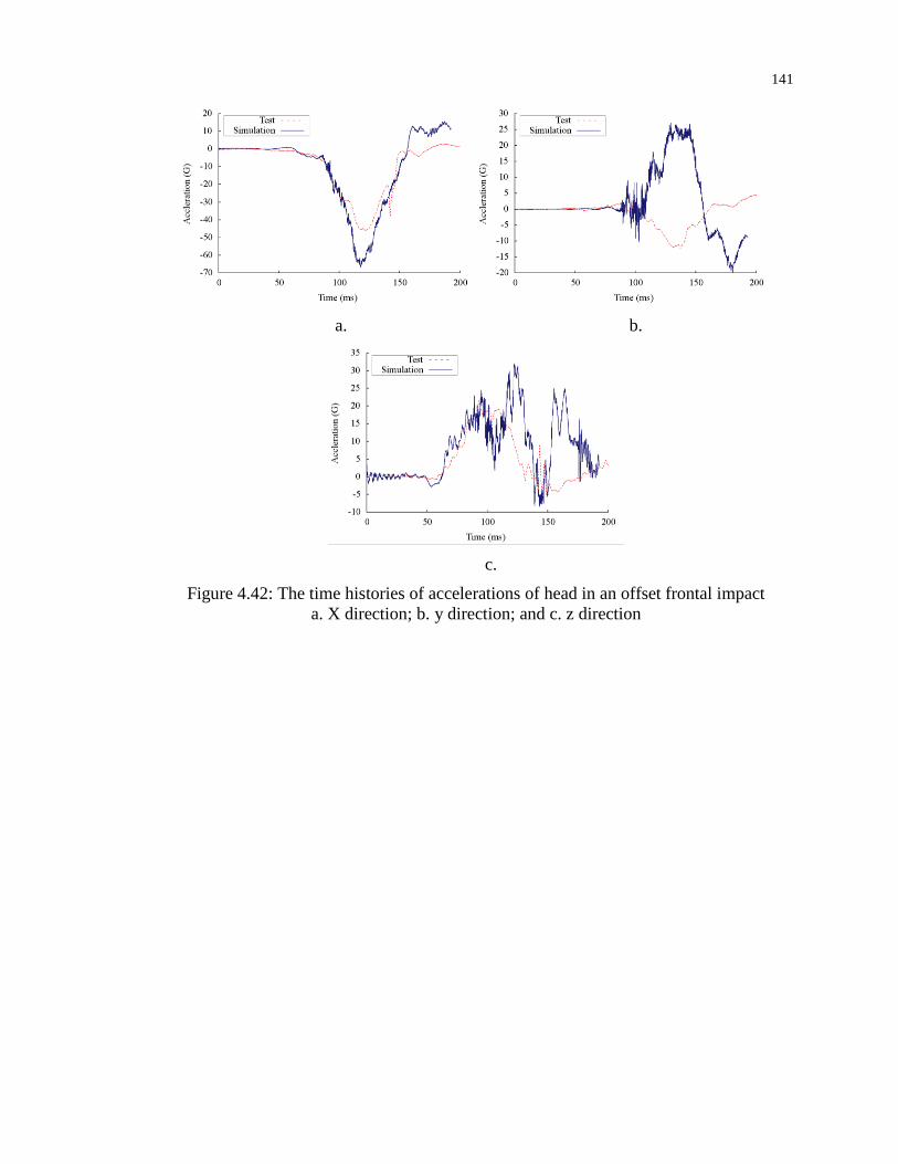
141
a. b.
c.
Figure 4.42: The time histories of accelerations of head in an offset frontal impact
a. X direction; b. y direction; and c. z direction
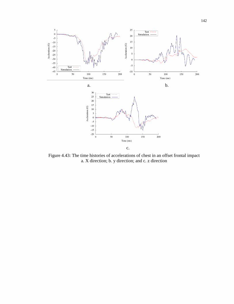
142
a. b.
c.
Figure 4.43: The time histories of accelerations of chest in an offset frontal impact
a. X direction; b. y direction; and c. z direction
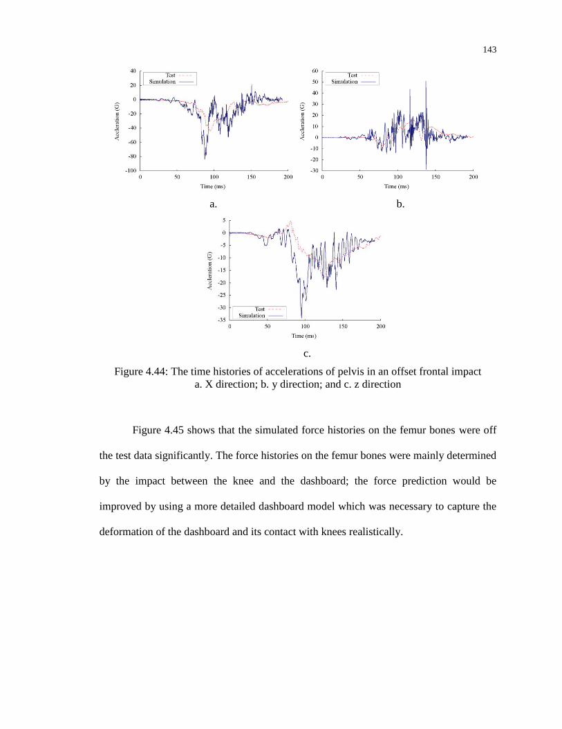
143
a. b.
c.
Figure 4.44: The time histories of accelerations of pelvis in an offset frontal impact
a. X direction; b. y direction; and c. z direction
Figure 4.45 shows that the simulated force histories on the femur bones were off
the test data significantly. The force histories on the femur bones were mainly determined
by the impact between the knee and the dashboard; the force prediction would be
improved by using a more detailed dashboard model which was necessary to capture the
deformation of the dashboard and its contact with knees realistically.
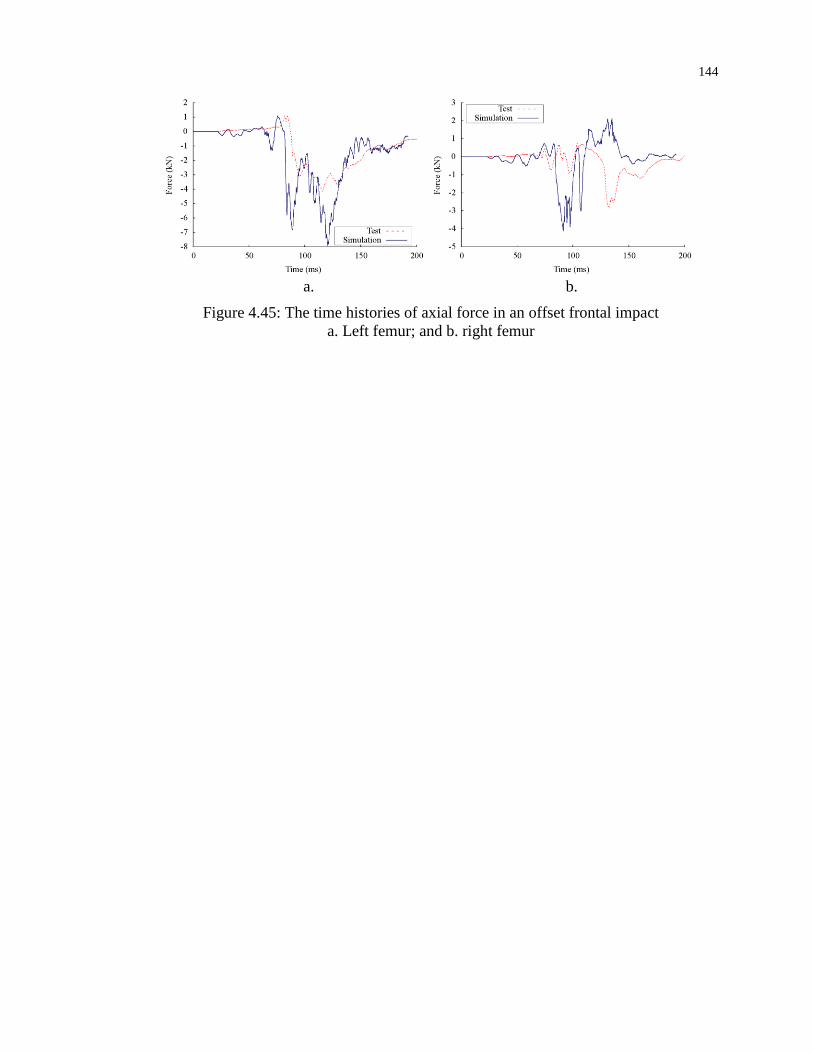
144
a. b.
Figure 4.45: The time histories of axial force in an offset frontal impact
a. Left femur; and b. right femur
CHAPTER 5: FINITE ELEMENT MODELING AND SIMULATION OF HIGHWAY
CRASHES
Miles of median barrier systems such as W-beam guardrails and cable median
barriers have been installed on the highway and shown to be effective in reducing the
roadway crashes. A successfully designed median barrier should be able to contain and
safely redirect the impacting vehicle. Crash with a median barrier is also expected to be
more forgiving so as to provide a greater chance of survivability than vehicle-vehicle
crashes and vehicle crashing into obstacles.
Most of the information about the safety performances of a median barrier is
obtained by crash testing and can be studied in details using crash simulations. The
impact tests/simulations will provide the basis for judging the structural adequacy,
occupant risk, and vehicle trajectory. For example, the barrier should contain and redirect
the vehicle and the vehicle should not penetrate, underride, or override the barrier. The
vehicle should also be upright and not overturn during engagement with the barrier and
should not be exposed with secondary impacts. To protect the occupant in the vehicle,
deformation of the occupant compartment that may cause serious injuries should not be
permitted.
Crash testing is a complicated process and involves a number of variables such as
weather, ground condition, vehicle, and barrier that all affect the test results. In an effort
to provide a uniform procedure and basis for evaluating the performance of longitudinal
barriers, MASH defined six different test levels (TL) each with specific testing vehicles,

146
impact speeds, and impact angles. Both 1,100-kg (2,420-lb) small passenger cars and
2,270-kg (5,000-lb) pickup trucks are used in all test levels. The impact speeds for test
levels 1, 2 and 3 are: TL-1 50 km/hr (31 mph), TL-2 70 km/hr (43 mph), and TL-3 100
km/hr (62 mph). In addition to the small passenger car and pickup truck, TL-4, -5 and -6
also use large-sized vehicles, i.e., a 10,000-kg (22,000-lb) single-unit truck for TL-4, a
36,000-kg (79,300-lb) tractor-van trailer for TL-5 and a 36,000-kg tractor-tank trailer for
TL-6. The impact speed used along with these large-sized vehicles is 80 km/hr (50 mph).
The impact angle is 15°. A successfully tested barrier system by these crash tests
indicates the confidence in the safety performance of the barrier system. However, they
should only be considered as necessary conditions but not sufficient conditions for a
successful median barrier design.
The ultimate goal of designing a median barrier system is to save life and
minimize the injury to the occupant. Although examining the vehicle responses and
barrier performances is helpful to assess the safety of an occupant in a crash, the occupant
responses should be directly examined. This is because, as pointed out by MASH, the
relationship between occupant risk and vehicle dynamics during interaction with roadside
safety hardware is very difficult to quantify. A safe vehicle response is a good indication
of occupant safety but not a guarantee. The idea of incorporating a crash test dummy in
crash testing of barrier systems serves as the means to directly evaluate the occupant
safety, because using a human being in a crash test is nearly impossible and not
encouraged. Incorporating a crash test dummy in full-scale crash testing of roadside
barriers is ideal but difficult due to the high cost, level of instrumentation, and required
expertise. As a result, using crash test dummy is encouraged but not required in the
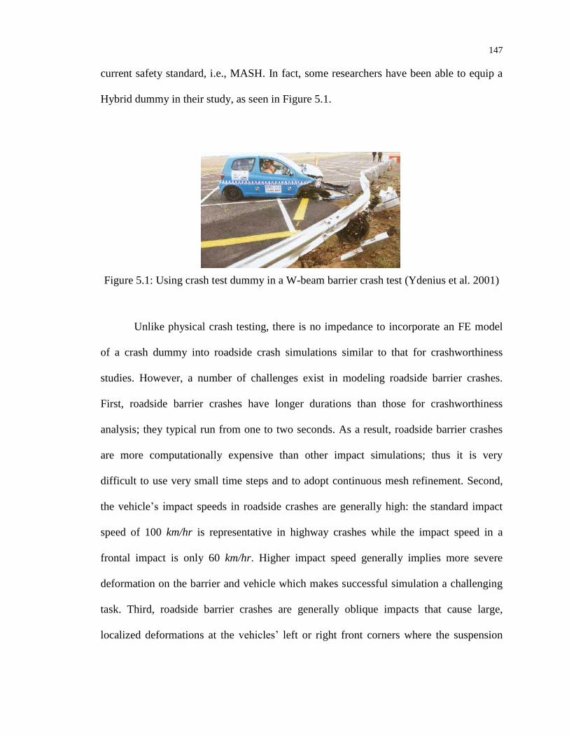
147
current safety standard, i.e., MASH. In fact, some researchers have been able to equip a
Hybrid dummy in their study, as seen in Figure 5.1.
Figure 5.1: Using crash test dummy in a W-beam barrier crash test (Ydenius et al. 2001)
Unlike physical crash testing, there is no impedance to incorporate an FE model
of a crash dummy into roadside crash simulations similar to that for crashworthiness
studies. However, a number of challenges exist in modeling roadside barrier crashes.
First, roadside barrier crashes have longer durations than those for crashworthiness
analysis; they typical run from one to two seconds. As a result, roadside barrier crashes
are more computationally expensive than other impact simulations; thus it is very
difficult to use very small time steps and to adopt continuous mesh refinement. Second,
the vehicle’s impact speeds in roadside crashes are generally high: the standard impact
speed of 100 km/hr is representative in highway crashes while the impact speed in a
frontal impact is only 60 km/hr. Higher impact speed generally implies more severe
deformation on the barrier and vehicle which makes successful simulation a challenging
task. Third, roadside barrier crashes are generally oblique impacts that cause large,
localized deformations at the vehicles’ left or right front corners where the suspension
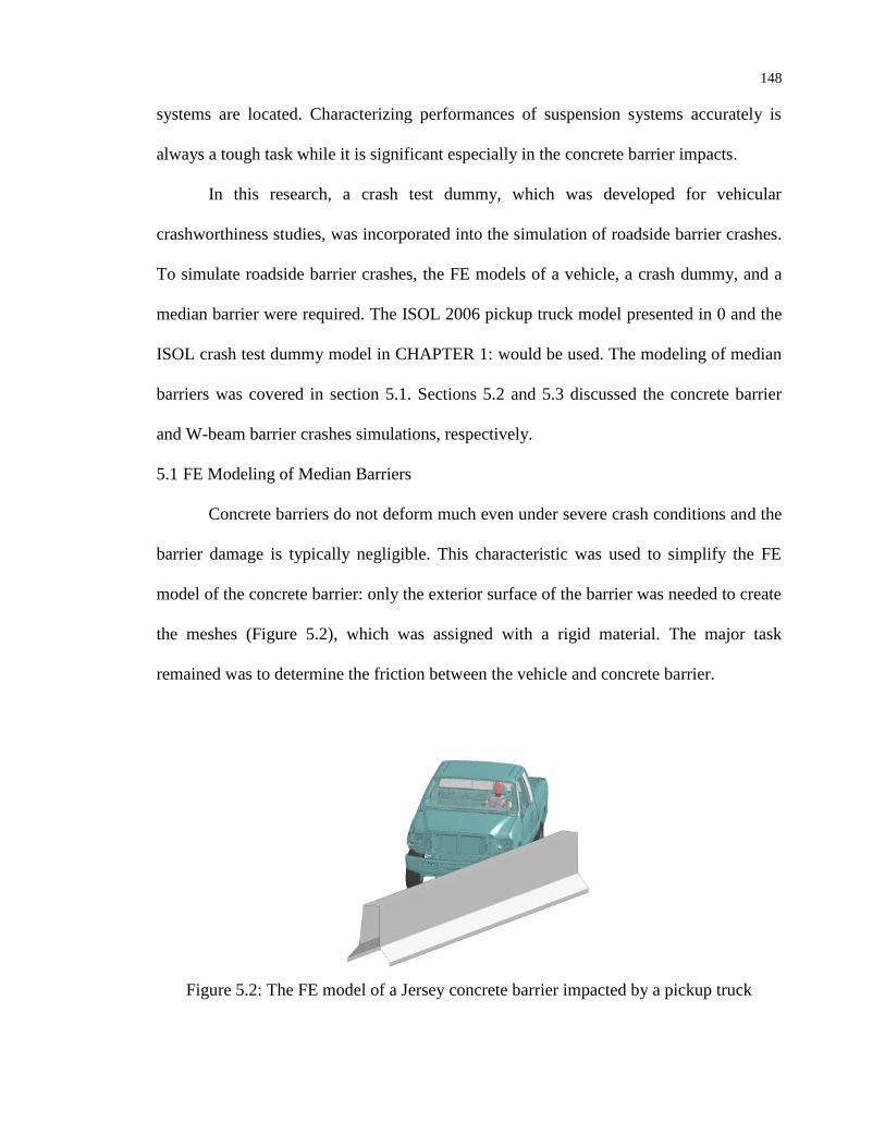
148
systems are located. Characterizing performances of suspension systems accurately is
always a tough task while it is significant especially in the concrete barrier impacts.
In this research, a crash test dummy, which was developed for vehicular
crashworthiness studies, was incorporated into the simulation of roadside barrier crashes.
To simulate roadside barrier crashes, the FE models of a vehicle, a crash dummy, and a
median barrier were required. The ISOL 2006 pickup truck model presented in 0 and the
ISOL crash test dummy model in CHAPTER 1: would be used. The modeling of median
barriers was covered in section 5.1. Sections 5.2 and 5.3 discussed the concrete barrier
and W-beam barrier crashes simulations, respectively.
5.1 FE Modeling of Median Barriers
Concrete barriers do not deform much even under severe crash conditions and the
barrier damage is typically negligible. This characteristic was used to simplify the FE
model of the concrete barrier: only the exterior surface of the barrier was needed to create
the meshes (Figure 5.2), which was assigned with a rigid material. The major task
remained was to determine the friction between the vehicle and concrete barrier.
Figure 5.2: The FE model of a Jersey concrete barrier impacted by a pickup truck
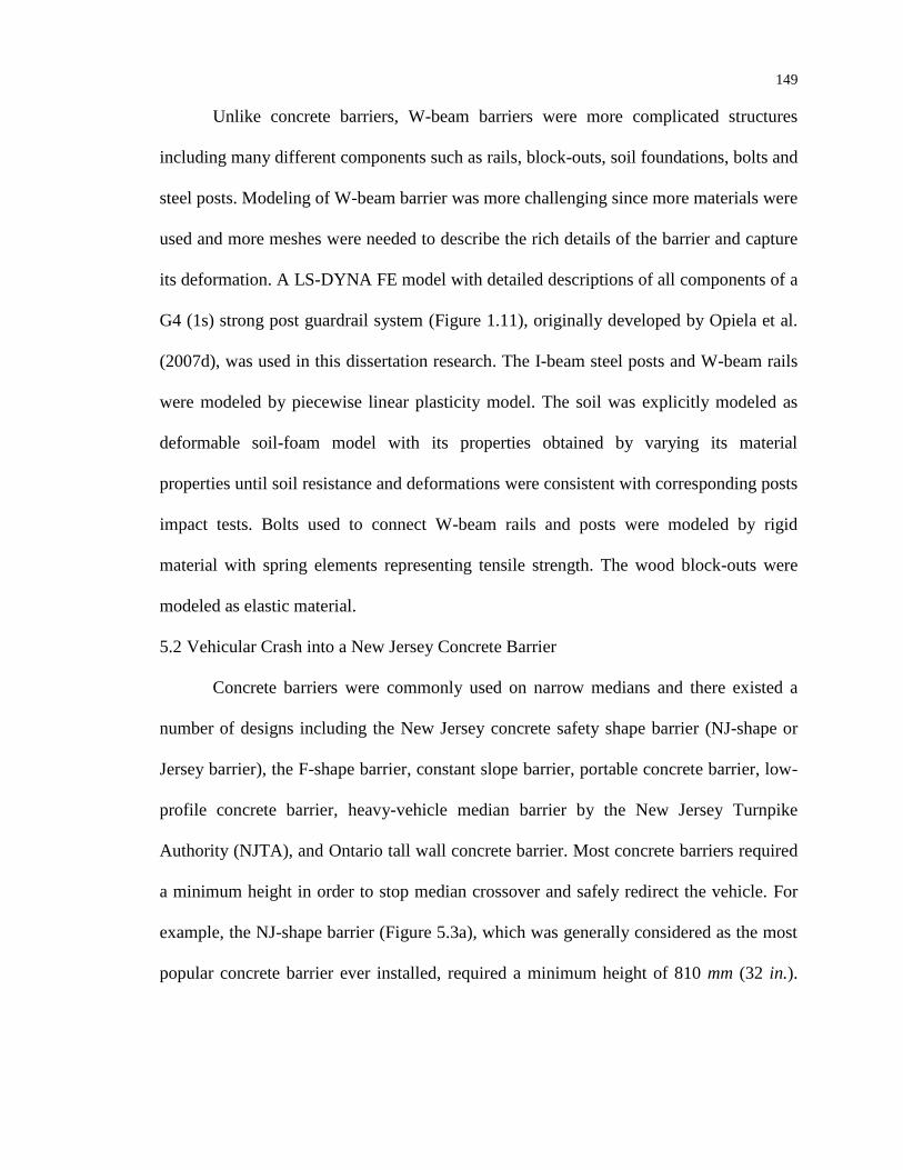
149
Unlike concrete barriers, W-beam barriers were more complicated structures
including many different components such as rails, block-outs, soil foundations, bolts and
steel posts. Modeling of W-beam barrier was more challenging since more materials were
used and more meshes were needed to describe the rich details of the barrier and capture
its deformation. A LS-DYNA FE model with detailed descriptions of all components of a
G4 (1s) strong post guardrail system (Figure 1.11), originally developed by Opiela et al.
(2007d), was used in this dissertation research. The I-beam steel posts and W-beam rails
were modeled by piecewise linear plasticity model. The soil was explicitly modeled as
deformable soil-foam model with its properties obtained by varying its material
properties until soil resistance and deformations were consistent with corresponding posts
impact tests. Bolts used to connect W-beam rails and posts were modeled by rigid
material with spring elements representing tensile strength. The wood block-outs were
modeled as elastic material.
5.2 Vehicular Crash into a New Jersey Concrete Barrier
Concrete barriers were commonly used on narrow medians and there existed a
number of designs including the New Jersey concrete safety shape barrier (NJ-shape or
Jersey barrier), the F-shape barrier, constant slope barrier, portable concrete barrier, low-
profile concrete barrier, heavy-vehicle median barrier by the New Jersey Turnpike
Authority (NJTA), and Ontario tall wall concrete barrier. Most concrete barriers required
a minimum height in order to stop median crossover and safely redirect the vehicle. For
example, the NJ-shape barrier (Figure 5.3a), which was generally considered as the most
popular concrete barrier ever installed, required a minimum height of 810 mm (32 in.).
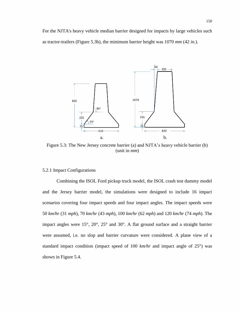
150
For the NJTA's heavy vehicle median barrier designed for impacts by large vehicles such
as tractor-trailers (Figure 5.3b), the minimum barrier height was 1070 mm (42 in.).
a. b.
Figure 5.3: The New Jersey concrete barrier (a) and NJTA’s heavy vehicle barrier (b)
(unit in mm)
5.2.1 Impact Configurations
Combining the ISOL Ford pickup truck model, the ISOL crash test dummy model
and the Jersey barrier model, the simulations were designed to include 16 impact
scenarios covering four impact speeds and four impact angles. The impact speeds were
50 km/hr (31 mph), 70 km/hr (43 mph), 100 km/hr (62 mph) and 120 km/hr (74 mph). The
impact angles were 15°, 20°, 25° and 30°. A flat ground surface and a straight barrier
were assumed, i.e. no slop and barrier curvature were considered. A plane view of a
standard impact condition (impact speed of 100 km/hr and impact angle of 25°) was
shown in Figure 5.4.
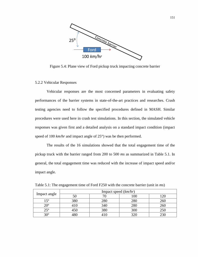
151
Figure 5.4: Plane view of Ford pickup truck impacting concrete barrier
5.2.2 Vehicular Responses
Vehicular responses are the most concerned parameters in evaluating safety
performances of the barrier systems in state-of-the-art practices and researches. Crash
testing agencies need to follow the specified procedures defined in MASH. Similar
procedures were used here in crash test simulations. In this section, the simulated vehicle
responses was given first and a detailed analysis on a standard impact condition (impact
speed of 100 km/hr and impact angle of 25°) was be then performed.
The results of the 16 simulations showed that the total engagement time of the
pickup truck with the barrier ranged from 200 to 500 ms as summarized in Table 5.1. In
general, the total engagement time was reduced with the increase of impact speed and/or
impact angle.
Table 5.1: The engagement time of Ford F250 with the concrete barrier (unit in ms)
Impact angle Impact speed (km/hr)
50 70 100 120
15º 380 280 280 260
20º 410 340 280 260
25º 450 380 300 250
30º 480 410 320 230
152
The yaw, pitch and roll of the vehicle, as defined in Figure 5.5, were used to
examine the vehicle’s orientation and stability during an impact. The yaw angle indicated
how much the vehicle was redirected, and the pitch and roll angle could be used to assess
the stability of the vehicle during the crash. A large pitch or roll angle implied unstable
vehicle behavior and as required by MASH the pitch and roll angles should not exceed
75°.
Figure 5.5 Definition of yaw, pitch and roll
Table 5.2 lists the maximum pitch and roll angles of all 16 simulated impacts. It
can be seen that all the impacts had acceptable pitch and roll angles except for the case
with impact speed of 100 km/hr and impact angle of 30°.
Table 5.2: The maximum pitch/roll angles of the Ford F250 impacting a concrete barrier
Impact angle Impact speed (km/hr)
50 70 100 120
15º 4.00/10.40 6.27/26.12 4.61/46.66 6.30/49.99
20º 5.80/15.20 7.13/32.60 8.59/52.64 4.71/59.62
25º 6.70/11.18 8.20/32.59 4.74/55.95 5.46/65.69
30º 6.38/13.90 7.31/49.16 9.58/107.49 11.52/71.13
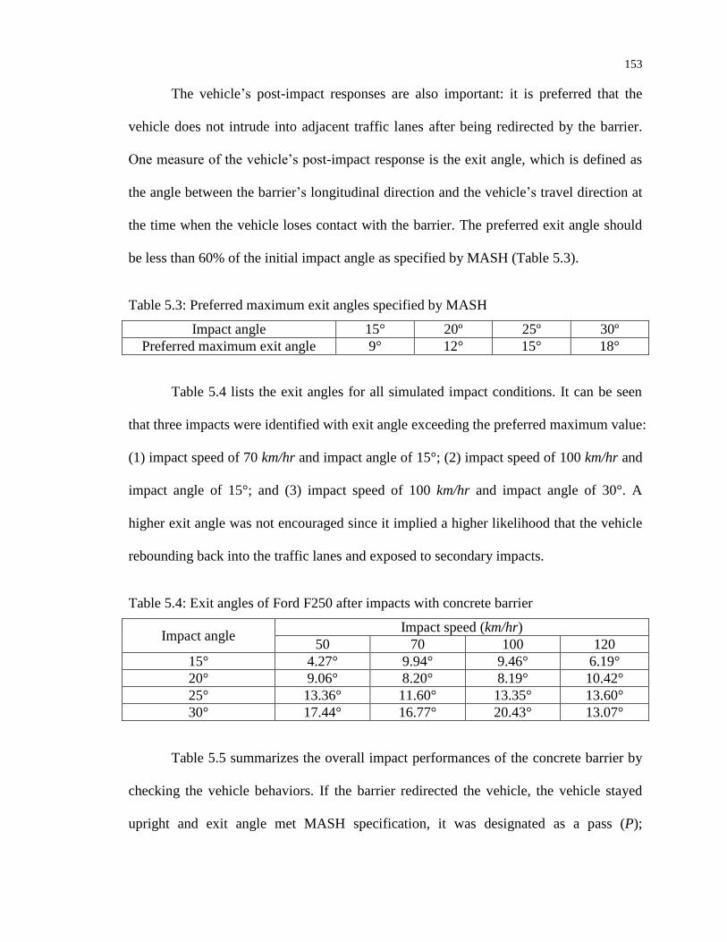
153
The vehicle’s post-impact responses are also important: it is preferred that the
vehicle does not intrude into adjacent traffic lanes after being redirected by the barrier.
One measure of the vehicle’s post-impact response is the exit angle, which is defined as
the angle between the barrier’s longitudinal direction and the vehicle’s travel direction at
the time when the vehicle loses contact with the barrier. The preferred exit angle should
be less than 60% of the initial impact angle as specified by MASH (Table 5.3).
Table 5.3: Preferred maximum exit angles specified by MASH
Impact angle 15° 20º 25º 30º
Preferred maximum exit angle 9° 12° 15° 18°
Table 5.4 lists the exit angles for all simulated impact conditions. It can be seen
that three impacts were identified with exit angle exceeding the preferred maximum value:
(1) impact speed of 70 km/hr and impact angle of 15°; (2) impact speed of 100 km/hr and
impact angle of 15°; and (3) impact speed of 100 km/hr and impact angle of 30°. A
higher exit angle was not encouraged since it implied a higher likelihood that the vehicle
rebounding back into the traffic lanes and exposed to secondary impacts.
Table 5.4: Exit angles of Ford F250 after impacts with concrete barrier
Impact angle Impact speed (km/hr)
50 70 100 120
15° 4.27° 9.94° 9.46° 6.19°
20° 9.06° 8.20° 8.19° 10.42°
25° 13.36° 11.60° 13.35° 13.60°
30° 17.44° 16.77° 20.43° 13.07°
Table 5.5 summarizes the overall impact performances of the concrete barrier by
checking the vehicle behaviors. If the barrier redirected the vehicle, the vehicle stayed
upright and exit angle met MASH specification, it was designated as a pass (P);
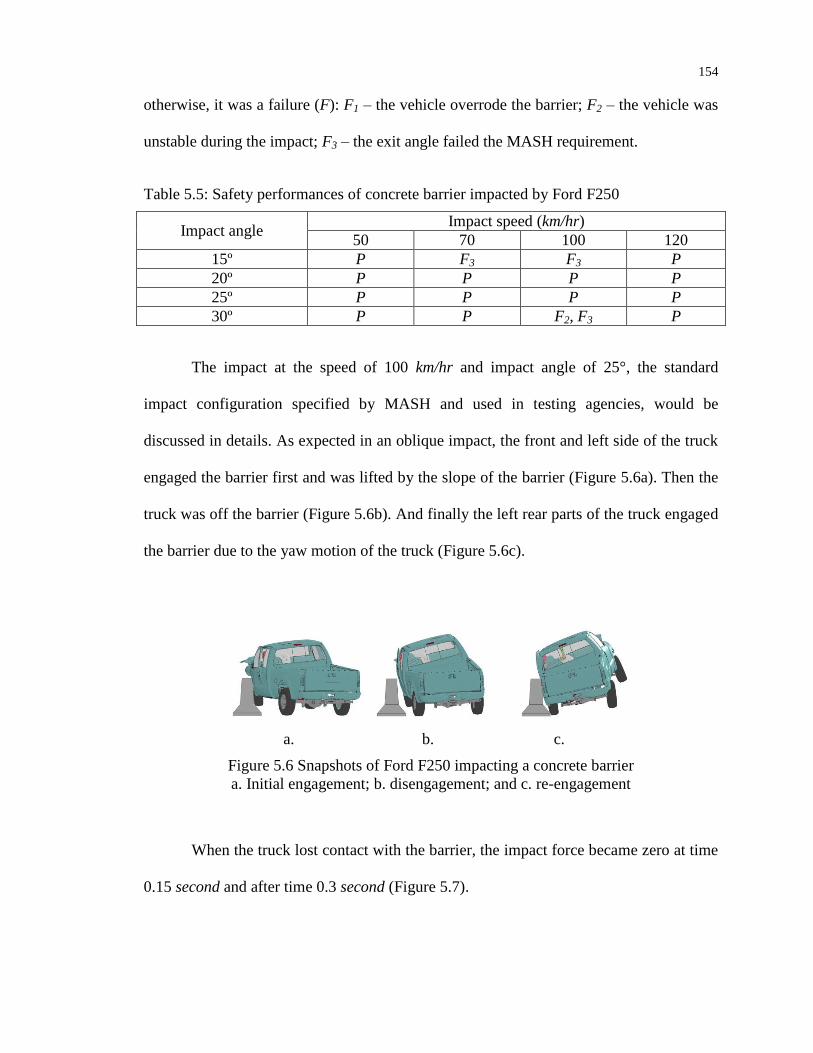
154
otherwise, it was a failure (F): F1 – the vehicle overrode the barrier; F2 – the vehicle was
unstable during the impact; F3 – the exit angle failed the MASH requirement.
Table 5.5: Safety performances of concrete barrier impacted by Ford F250
Impact angle Impact speed (km/hr)
50 70 100 120
15º P F3 F3 P
20º P P P P
25º P P P P
30º P P F2, F3 P
The impact at the speed of 100 km/hr and impact angle of 25°, the standard
impact configuration specified by MASH and used in testing agencies, would be
discussed in details. As expected in an oblique impact, the front and left side of the truck
engaged the barrier first and was lifted by the slope of the barrier (Figure 5.6a). Then the
truck was off the barrier (Figure 5.6b). And finally the left rear parts of the truck engaged
the barrier due to the yaw motion of the truck (Figure 5.6c).
a. b. c.
Figure 5.6 Snapshots of Ford F250 impacting a concrete barrier
a. Initial engagement; b. disengagement; and c. re-engagement
When the truck lost contact with the barrier, the impact force became zero at time
0.15 second and after time 0.3 second (Figure 5.7).
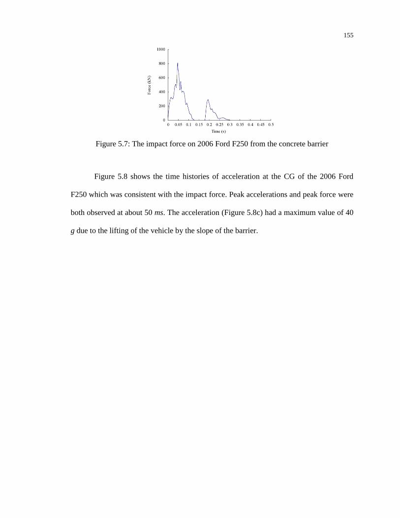
155
Figure 5.7: The impact force on 2006 Ford F250 from the concrete barrier
Figure 5.8 shows the time histories of acceleration at the CG of the 2006 Ford
F250 which was consistent with the impact force. Peak accelerations and peak force were
both observed at about 50 ms. The acceleration (Figure 5.8c) had a maximum value of 40
g due to the lifting of the vehicle by the slope of the barrier.
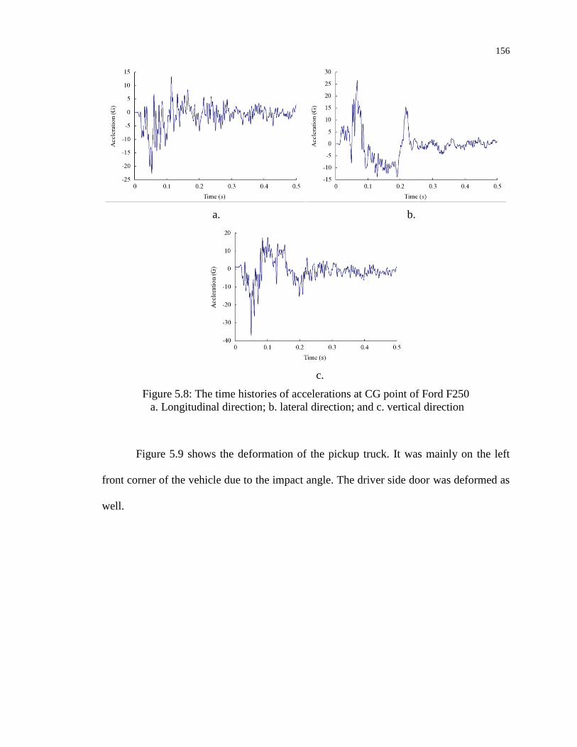
156
a. b.
c.
Figure 5.8: The time histories of accelerations at CG point of Ford F250
a. Longitudinal direction; b. lateral direction; and c. vertical direction
Figure 5.9 shows the deformation of the pickup truck. It was mainly on the left
front corner of the vehicle due to the impact angle. The driver side door was deformed as
well.
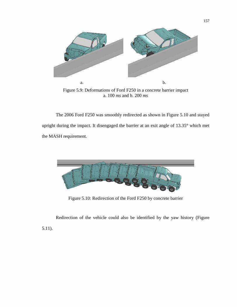
157
a. b.
Figure 5.9: Deformations of Ford F250 in a concrete barrier impact
a. 100 ms and b. 200 ms
The 2006 Ford F250 was smoothly redirected as shown in Figure 5.10 and stayed
upright during the impact. It disengaged the barrier at an exit angle of 13.35° which met
the MASH requirement.
Figure 5.10: Redirection of the Ford F250 by concrete barrier
Redirection of the vehicle could also be identified by the yaw history (Figure
5.11).

158
Figure 5.11: The time histories of yaw, pitch and roll of Ford F250 during an impact with
concrete barrier
5.2.3 Occupant Responses
In contrast to vehicular responses, occupant responses are barely evaluated in
crash testing and/or crash simulations. In fact, there is no available clearly defined
evaluation criteria used in roadside barrier crashes due to the absence of crash test
dummy. In this section, the occupant responses were presented for the standard impact
condition (impact speed of 100 km/hr and impact angle of 25°).
The airbag, deployed in a controlled time of 40 ms, had no contact with the
dummy and provided no protection to the occupant due to the impact angle. The contact
force between the dummy and airbag is therefore zero during the impact as shown in
Figure 5.12.

159
Figure 5.12: Impact force on the dummy from the airbag in a concrete barrier impact
Figure 5.13 shows the responses of seat belt. The seat belt was the only active
restraint during the impact. At around 110 ms both the shoulder belt force and lap belt
force reached their maximum, 3.5 kN and 5.5 kN, respectively.
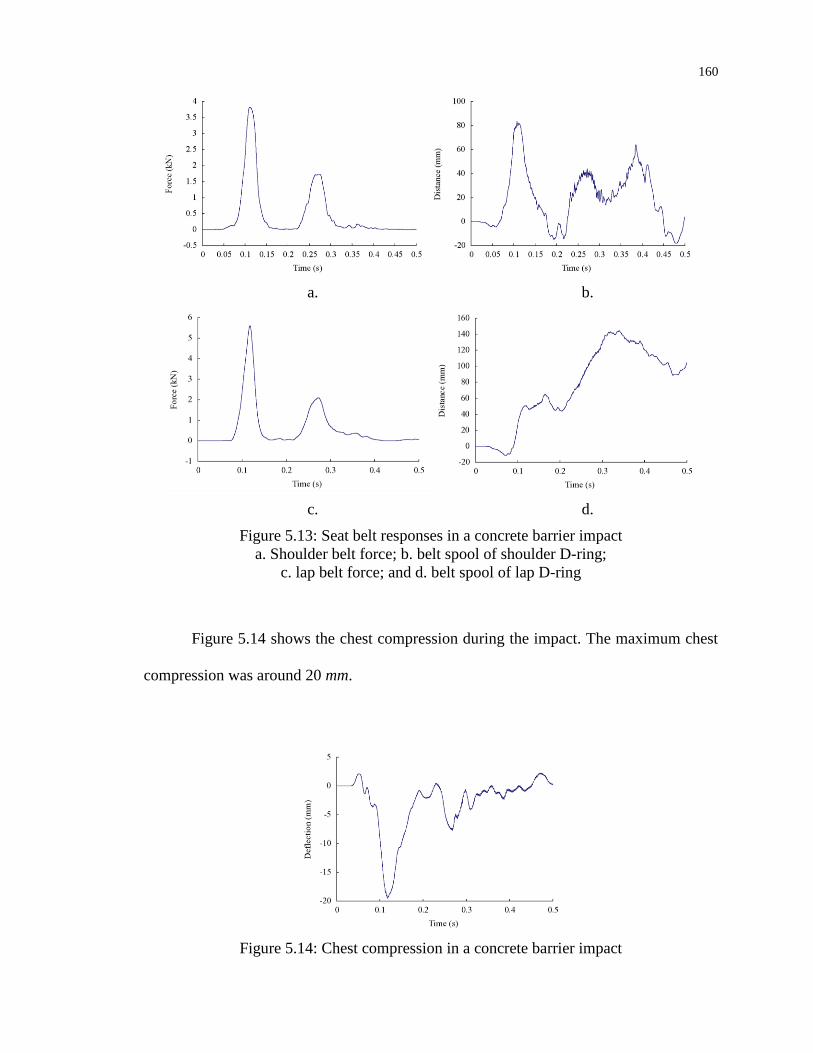
160
a. b.
c. d.
Figure 5.13: Seat belt responses in a concrete barrier impact
a. Shoulder belt force; b. belt spool of shoulder D-ring;
c. lap belt force; and d. belt spool of lap D-ring
Figure 5.14 shows the chest compression during the impact. The maximum chest
compression was around 20 mm.
Figure 5.14: Chest compression in a concrete barrier impact
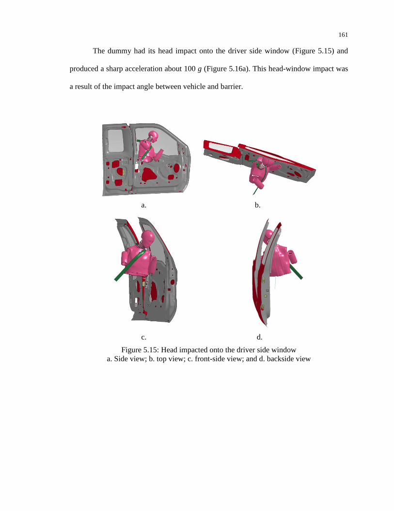
161
The dummy had its head impact onto the driver side window (Figure 5.15) and
produced a sharp acceleration about 100 g (Figure 5.16a). This head-window impact was
a result of the impact angle between vehicle and barrier.
a. b.
c. d.
Figure 5.15: Head impacted onto the driver side window
a. Side view; b. top view; c. front-side view; and d. backside view
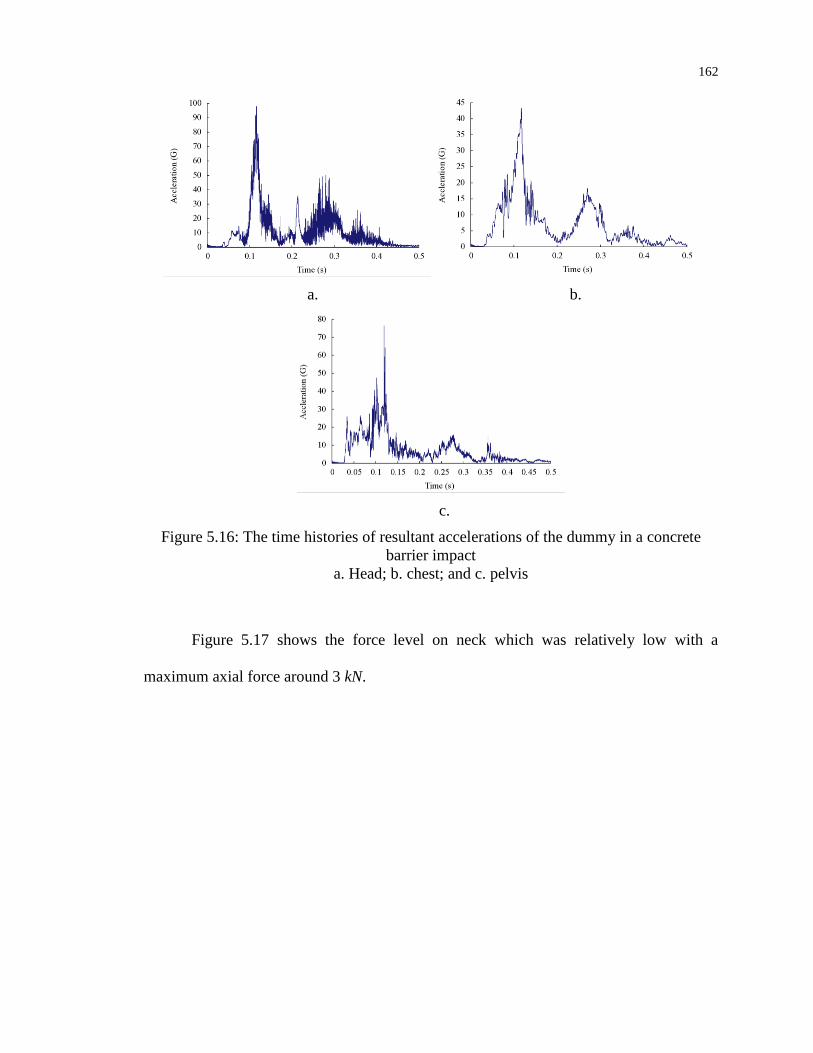
162
a. b.
c.
Figure 5.16: The time histories of resultant accelerations of the dummy in a concrete
barrier impact
a. Head; b. chest; and c. pelvis
Figure 5.17 shows the force level on neck which was relatively low with a
maximum axial force around 3 kN.
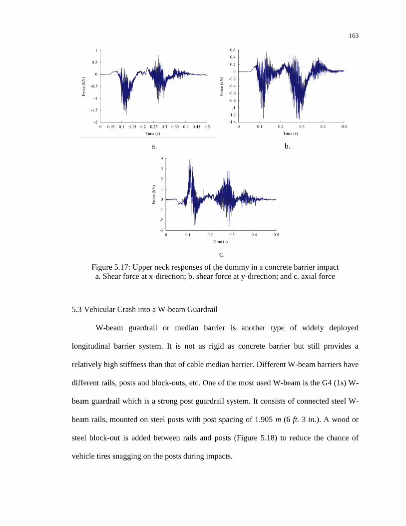
163
a. b.
c.
Figure 5.17: Upper neck responses of the dummy in a concrete barrier impact
a. Shear force at x-direction; b. shear force at y-direction; and c. axial force
5.3 Vehicular Crash into a W-beam Guardrail
W-beam guardrail or median barrier is another type of widely deployed
longitudinal barrier system. It is not as rigid as concrete barrier but still provides a
relatively high stiffness than that of cable median barrier. Different W-beam barriers have
different rails, posts and block-outs, etc. One of the most used W-beam is the G4 (1s) W-
beam guardrail which is a strong post guardrail system. It consists of connected steel W-
beam rails, mounted on steel posts with post spacing of 1.905 m (6 ft. 3 in.). A wood or
steel block-out is added between rails and posts (Figure 5.18) to reduce the chance of
vehicle tires snagging on the posts during impacts.

164
a. b.
Figure 5.18: A post of G4 (1s) W-beam barrier
a. Front-side view; and b. backside view
5.3.1 Impact Configurations
The impact configurations with W-beam guardrail were the same as that in
concrete barrier impacts in section 5.2.1 with the exception that the 15° impact angle used
in the concrete barrier simulations was dropped. The simulations included 12 impacts
with 4 different speeds and 3 different impact angles in accordance to MASH test levels
specifications. The impact speeds were 50 km/hr (31.1 mph), 70 km/hr (43.5 mph), 100
km/hr (62.1 mph) and 120 km/hr (74.6 mph). The impact angles included 20°, 25° and
30°. In all impacts, the pickup was positioned at about 1/3 of the overall length of the
barrier from upstream as shown in Figure 5.19.
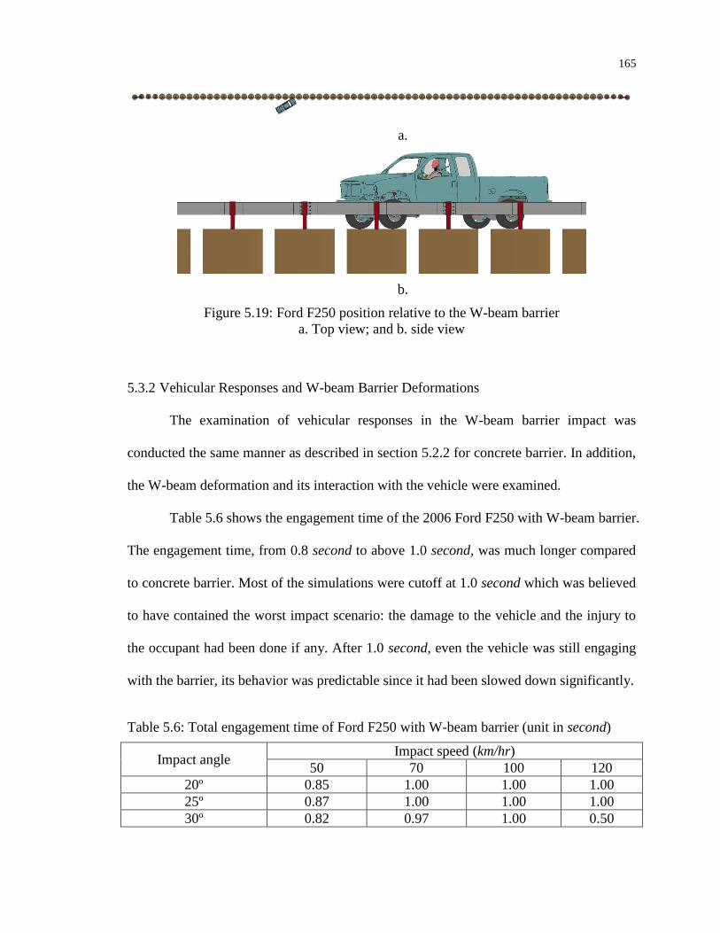
165
a.
b.
Figure 5.19: Ford F250 position relative to the W-beam barrier
a. Top view; and b. side view
5.3.2 Vehicular Responses and W-beam Barrier Deformations
The examination of vehicular responses in the W-beam barrier impact was
conducted the same manner as described in section 5.2.2 for concrete barrier. In addition,
the W-beam deformation and its interaction with the vehicle were examined.
Table 5.6 shows the engagement time of the 2006 Ford F250 with W-beam barrier.
The engagement time, from 0.8 second to above 1.0 second, was much longer compared
to concrete barrier. Most of the simulations were cutoff at 1.0 second which was believed
to have contained the worst impact scenario: the damage to the vehicle and the injury to
the occupant had been done if any. After 1.0 second, even the vehicle was still engaging
with the barrier, its behavior was predictable since it had been slowed down significantly.
Table 5.6: Total engagement time of Ford F250 with W-beam barrier (unit in second)
Impact angle Impact speed (km/hr)
50 70 100 120
20º 0.85 1.00 1.00 1.00
25º 0.87 1.00 1.00 1.00
30º 0.82 0.97 1.00 0.50
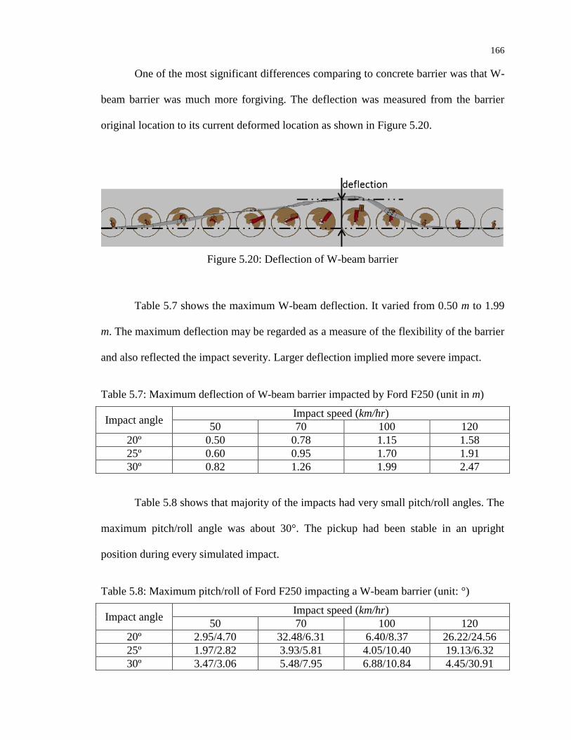
166
One of the most significant differences comparing to concrete barrier was that W-
beam barrier was much more forgiving. The deflection was measured from the barrier
original location to its current deformed location as shown in Figure 5.20.
Figure 5.20: Deflection of W-beam barrier
Table 5.7 shows the maximum W-beam deflection. It varied from 0.50 m to 1.99
m. The maximum deflection may be regarded as a measure of the flexibility of the barrier
and also reflected the impact severity. Larger deflection implied more severe impact.
Table 5.7: Maximum deflection of W-beam barrier impacted by Ford F250 (unit in m)
Impact angle Impact speed (km/hr)
50 70 100 120
20º 0.50 0.78 1.15 1.58
25º 0.60 0.95 1.70 1.91
30º 0.82 1.26 1.99 2.47
Table 5.8 shows that majority of the impacts had very small pitch/roll angles. The
maximum pitch/roll angle was about 30°. The pickup had been stable in an upright
position during every simulated impact.
Table 5.8: Maximum pitch/roll of Ford F250 impacting a W-beam barrier (unit: °)
Impact angle Impact speed (km/hr)
50 70 100 120
20º 2.95/4.70 32.48/6.31 6.40/8.37 26.22/24.56
25º 1.97/2.82 3.93/5.81 4.05/10.40 19.13/6.32
30º 3.47/3.06 5.48/7.95 6.88/10.84 4.45/30.91

167
Strictly speaking, no smooth redirection of the vehicle had been observed in all
impacts. There was vehicle snagging with the W-beam barrier as shown in Figure 5.21b
in majority of the impacts because rail and/or post often got behind the wheel and got
tangled (Figure 5.21a, Figure 5.22a). The entanglement diminished greatly the chance of
smooth vehicle redirection. The vehicle turned away rather than smoothly redirected by
the barrier (Figure 5.21b) and this behavior was termed as vehicle spin-out. Occasionally
entanglement between wheel and W-beam helped to prevent the vehicle override the
barrier as in Figure 5.22a where the front wheels entangled with the barrier. However,
this should be regarded as an exception rather than a desired feature of a successful
barrier design.
a. b.
Figure 5.21: Ford F250 spinning away from W-beam barrier
a. Isometric view; and b. top view

168
a. b.
Figure 5.22: Wheel of 2006 Ford F250 tangled with W-beam barrier
a. Isometric view; and b. top view
Table 5.9 lists exit angles for all the W-beam barrier impacts. As a result of
vehicle spin-out, majority of the impacts had a negative exit angle. Negative sign in front
of the exit angles implied a vehicle spin-out. If the vehicle was still in contact with W-
beam barrier at the conclusion of the simulation, calculation of exit angle was skipped.
Table 5.9: Exit angles of Ford F250 after impacts with W-beam barrier
Impact angle Impact speed (km/hr)
50 70 100 120
20° -8° - - -
25° -12° -17° - -
30° -45° -60° -40° -
The W-beam barrier contained the vehicle and prevented it from overriding in
majority of the impacts. There was one impact as shown in Figure 5.23 where the Ford
F250 overrode the barrier at an impact speed of 120 km/hr and impact angle of 30°.

169
a. b.
c. d.
Figure 5.23: Ford F250 overrode W-beam barrier at an impact speed of 120 km/hr and
impact angle of 30°
a. 149 ms; b. 349 ms; c. 384 ms and d. 502 ms
Table 5.10 summarizes the impact performances of the W-beam barrier. The exit
angles for all of the simulations were considered acceptable despite vehicle spin-out, i.e.
vehicle spin-out was not considered to fail the testing.
Table 5.10: The safety performance of W-beam barrier impacted by Ford F250
Impact angle Impact speed (km/hr)
50 70 100 120
20º P P P P
25º P P P P
30º P P P F1
The impact at the speed of 100 km/hr and impact angle of 25°, the standard
impact configuration specified by MASH and used in testing agencies, would again be
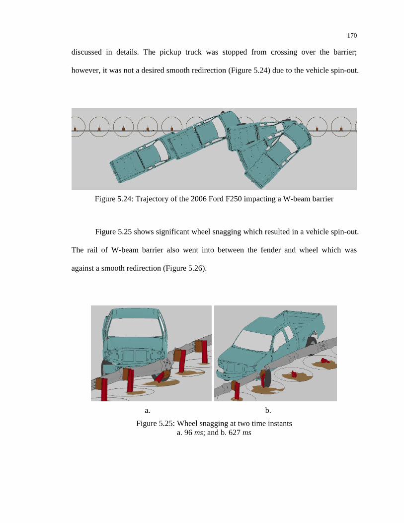
170
discussed in details. The pickup truck was stopped from crossing over the barrier;
however, it was not a desired smooth redirection (Figure 5.24) due to the vehicle spin-out.
Figure 5.24: Trajectory of the 2006 Ford F250 impacting a W-beam barrier
Figure 5.25 shows significant wheel snagging which resulted in a vehicle spin-out.
The rail of W-beam barrier also went into between the fender and wheel which was
against a smooth redirection (Figure 5.26).
a. b.
Figure 5.25: Wheel snagging at two time instants
a. 96 ms; and b. 627 ms
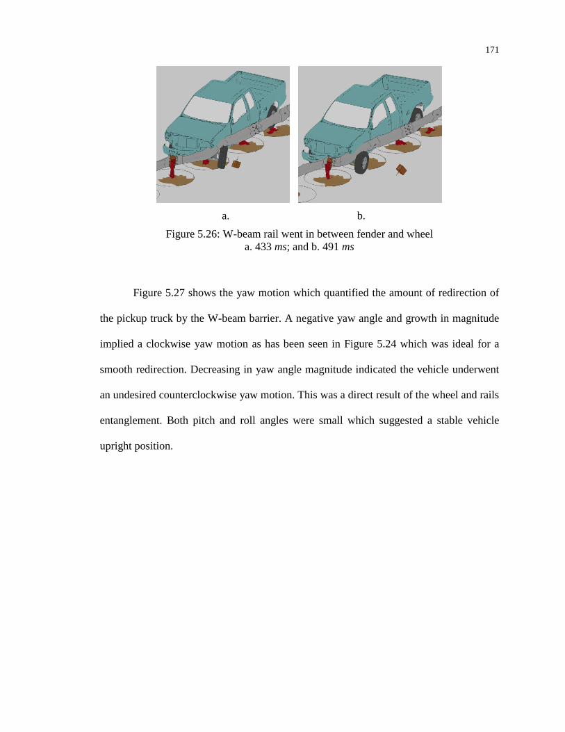
171
a. b.
Figure 5.26: W-beam rail went in between fender and wheel
a. 433 ms; and b. 491 ms
Figure 5.27 shows the yaw motion which quantified the amount of redirection of
the pickup truck by the W-beam barrier. A negative yaw angle and growth in magnitude
implied a clockwise yaw motion as has been seen in Figure 5.24 which was ideal for a
smooth redirection. Decreasing in yaw angle magnitude indicated the vehicle underwent
an undesired counterclockwise yaw motion. This was a direct result of the wheel and rails
entanglement. Both pitch and roll angles were small which suggested a stable vehicle
upright position.
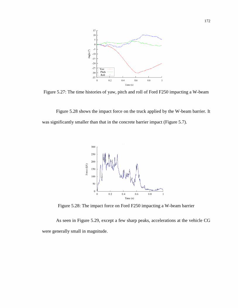
172
Figure 5.27: The time histories of yaw, pitch and roll of Ford F250 impacting a W-beam
Figure 5.28 shows the impact force on the truck applied by the W-beam barrier. It
was significantly smaller than that in the concrete barrier impact (Figure 5.7).
Figure 5.28: The impact force on Ford F250 impacting a W-beam barrier
As seen in Figure 5.29, except a few sharp peaks, accelerations at the vehicle CG
were generally small in magnitude.
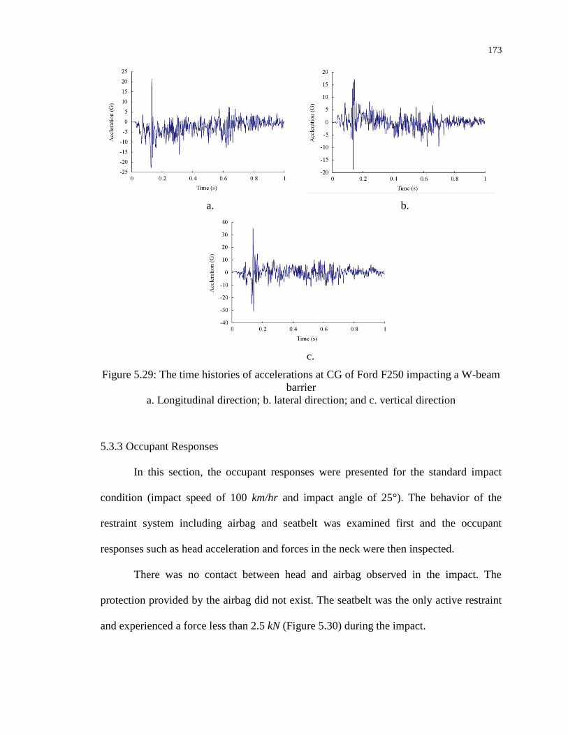
173
a. b.
c.
Figure 5.29: The time histories of accelerations at CG of Ford F250 impacting a W-beam
barrier
a. Longitudinal direction; b. lateral direction; and c. vertical direction
5.3.3 Occupant Responses
In this section, the occupant responses were presented for the standard impact
condition (impact speed of 100 km/hr and impact angle of 25°). The behavior of the
restraint system including airbag and seatbelt was examined first and the occupant
responses such as head acceleration and forces in the neck were then inspected.
There was no contact between head and airbag observed in the impact. The
protection provided by the airbag did not exist. The seatbelt was the only active restraint
and experienced a force less than 2.5 kN (Figure 5.30) during the impact.
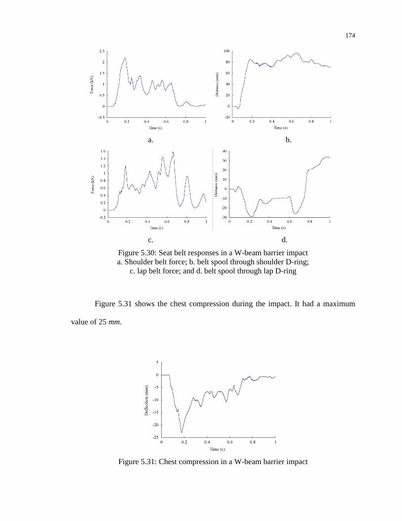
174
a. b.
c. d.
Figure 5.30: Seat belt responses in a W-beam barrier impact
a. Shoulder belt force; b. belt spool through shoulder D-ring;
c. lap belt force; and d. belt spool through lap D-ring
Figure 5.31 shows the chest compression during the impact. It had a maximum
value of 25 mm.
Figure 5.31: Chest compression in a W-beam barrier impact
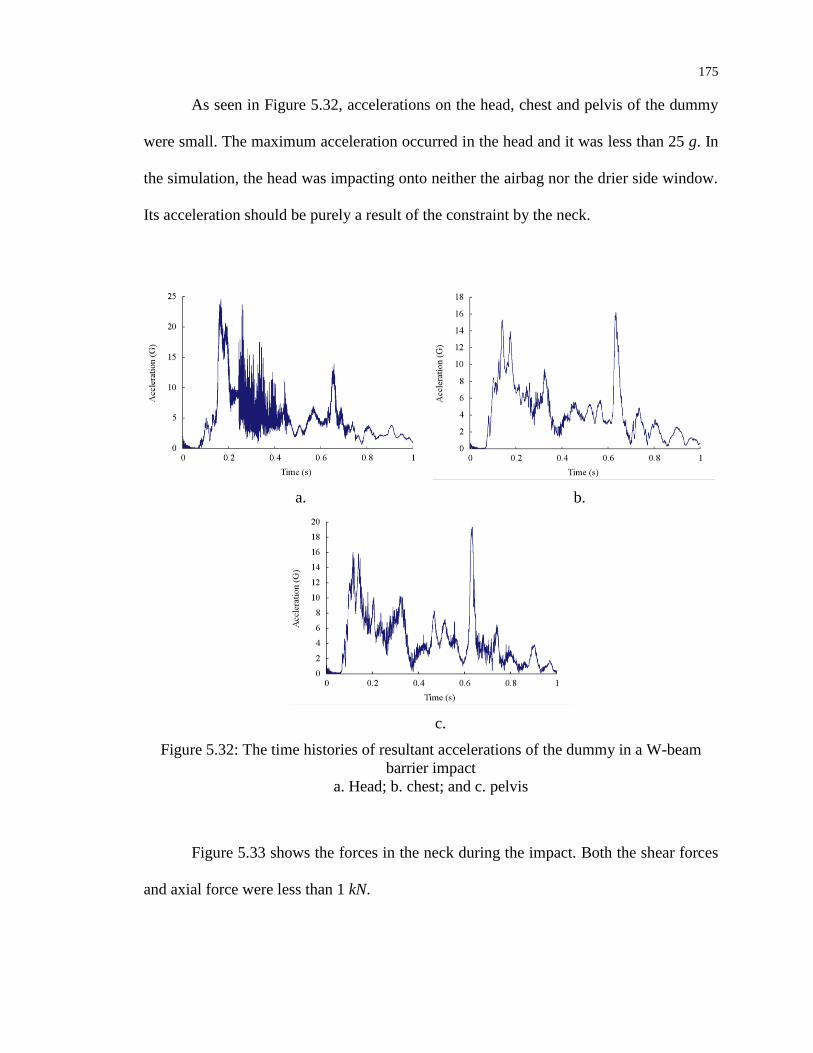
175
As seen in Figure 5.32, accelerations on the head, chest and pelvis of the dummy
were small. The maximum acceleration occurred in the head and it was less than 25 g. In
the simulation, the head was impacting onto neither the airbag nor the drier side window.
Its acceleration should be purely a result of the constraint by the neck.
a. b.
c.
Figure 5.32: The time histories of resultant accelerations of the dummy in a W-beam
barrier impact
a. Head; b. chest; and c. pelvis
Figure 5.33 shows the forces in the neck during the impact. Both the shear forces
and axial force were less than 1 kN.
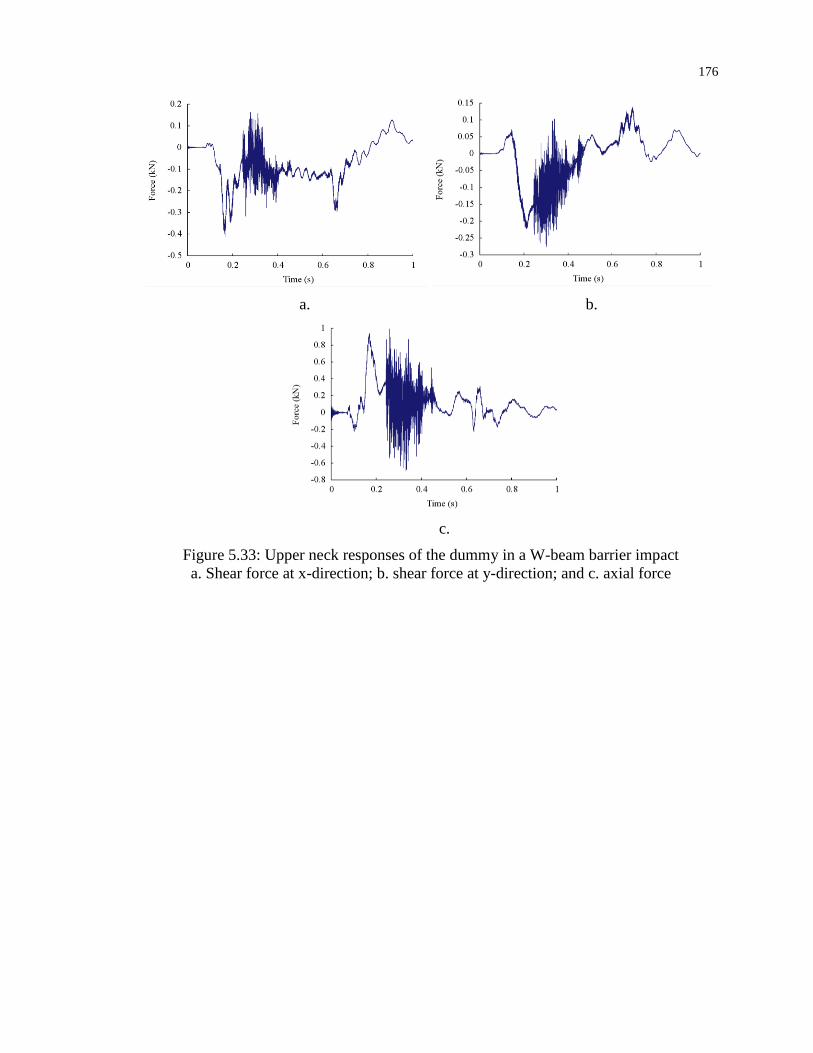
176
a. b.
c.
Figure 5.33: Upper neck responses of the dummy in a W-beam barrier impact
a. Shear force at x-direction; b. shear force at y-direction; and c. axial force
CHAPTER 6: ANALYSIS OF OCCUPANT INJURIES IN HIGHWAY CRASHES
Millions of people worldwide are injured in automotive crashes each year. There
were 32,367 people killed and 2.22 million people injured in the U.S. in 2011 from
5,338,000 reported motor vehicle crashes (NHTSA 2013). It is therefore of great
significance to comprehend the mechanism of occupant injury in automotive crashes, i.e.
it is necessary to study the parameters that can be used to assess the occupant responses
such as accelerations, stresses, and strains, and to determine their roles in causing certain
injuries to the human body so as to establish proper injury criteria for estimating the level
of injury severity.
6.1 Occupants Injuries and Injury Criteria
Occupant injuries in general include injuries of head, neck, chest, pelvis and
lower extremities. Each type of injury refers to a different individual body part and has its
own mechanism. To assess occupant injuries, injury criteria should be established for
each type of injury. However, directly evaluation of injury criteria on human body is
nearly impractical. Using crash test dummies is the common practice (Nyquist et al.
1980). Crash test dummies are instrumented to record data about its dynamic behavior in
vehicle impacts testing. Injury level is analyzed based on measured quantities. Due to
their good repeatability and biofidelity, crash test dummies are often used to help
establish injury criteria which are used to evaluate effectiveness of occupant protection
system in vehicle collisions. These ATD-based injury criteria are essential to
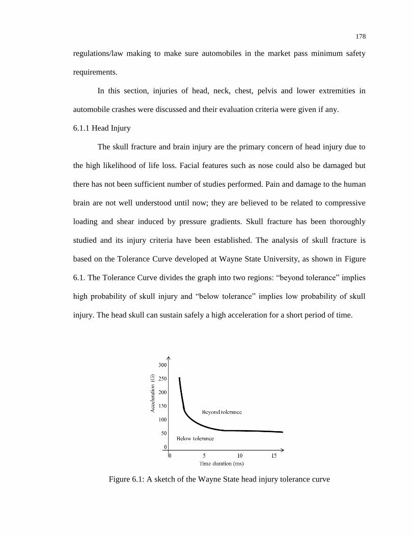
178
regulations/law making to make sure automobiles in the market pass minimum safety
requirements.
In this section, injuries of head, neck, chest, pelvis and lower extremities in
automobile crashes were discussed and their evaluation criteria were given if any.
6.1.1 Head Injury
The skull fracture and brain injury are the primary concern of head injury due to
the high likelihood of life loss. Facial features such as nose could also be damaged but
there has not been sufficient number of studies performed. Pain and damage to the human
brain are not well understood until now; they are believed to be related to compressive
loading and shear induced by pressure gradients. Skull fracture has been thoroughly
studied and its injury criteria have been established. The analysis of skull fracture is
based on the Tolerance Curve developed at Wayne State University, as shown in Figure
6.1. The Tolerance Curve divides the graph into two regions: “beyond tolerance” implies
high probability of skull injury and “below tolerance” implies low probability of skull
injury. The head skull can sustain safely a high acceleration for a short period of time.
Figure 6.1: A sketch of the Wayne State head injury tolerance curve

179
The injury criteria adopted by the U.S. federal government in FMVSS No. 208 is
the HIC developed by Versace (1971). The HIC is defined as
2
1
2.5
2 1
2 1
t
ta t dt
HIC Max t tt t
(6.1)
where is the resultant acceleration on the head measured in multiples of the
gravitational acceleration (g), and and are two time instants with t1 occurring before
t2. By the definition (6.1), HIC depends on the time interval and acceleration
history The most commonly used HIC is the , which is calculated using an
interval of 15 ms, that is, ms.
The probability of skull fracture is given by Hertz (1993) as
2ln 6.96352
0.84664 21
2
HICt
p HIC e dt
(6.2)
Using Eq. (6.2), the probability of skull fracture associated with an HIC15 of 700 is
determined to be 31%.
The skull is less likely fractured in the case of a small HIC; an intact skull
generally provides good protection to the brain but this is not a guarantee for zero brain
injury, because brain injury may occur without a skull fracture. The HIC serves as a
direct measurement of skull fracture, but not a direct measurement for brain injury. For
example, the rotational acceleration of the brain relative to the skull may cause brain
injury while not causing skull fracture. In the absence of rotational accelerations, the HIC
can still be used as a valid assessment for the effects under translational accelerations.
Currently, no substitute criteria have been proven better than the HIC and the HIC is still
used in federal regulations.

180
6.1.2 Neck Injury
Neck injury usually refers to damage to the spinal cord. Injuries of the neck spinal
cord typically result from a combination of axial and bending loads. There are currently
no widely accepted criteria established for neck injury due to the geometrical and
structural complexities. In a simple form, neck could be modeled as a slender column or
beam. Table 6.1 gives the allowable axial forces and bending moments on the neck to
avoid neck injuries.
Table 6.1: Allowable neck loading specified by FMVSS No. 208
Loading Allowable maximum
Axial compression 4000 N
Axial tension 3300 N
Shear force 3100 N
Flexion bending moment 190 Nm
Extension bending moment 57 Nm
Based directly on human limits rather than from dummy measurements maximum
acceptable flexion and extension bending moments were developed by Mertz and Patrick
(1971) according to sled tests conducted on volunteers and cadaver subjects. As in most
researches volunteer tests only provided data up to the pain threshold, and cadaver tests
were used to establish the limits for serious injuries. Compression in the neck usually
occurs in rollover accidents in which the body weight is applied to the head via neck.
Based on measurements made with Hybrid III dummy under impacts of a tackling block
that was reported to cause serious head and neck injuries among American football
players, Mertz et al. (1978) investigated the neck responses and established a maximum
value of 4-kN for axial compressive neck loading. The current tolerance levels, 3.3-kN for
tension and 3-kN for shear, were developed by Nyquist et al. (1980). They used a Hybrid

181
III 50% male dummy with 3-point belt to reconstruct real-world collisions and correlated
the test results with occupants’ field injuries.
6.1.3 Thorax Injury
Thorax, especially the rib cage and thoracic spine, protects the internal organs.
Fracture of the ribs or spines and impact waves are threatening to those thorax housed
tissues. In automotive crashes, chest compression is largely due to seat belt loading.
Based on cadaver tests, Eppinger et al. (1984) developed the TTI criteria that was defined
as half of the sum of peak chest acceleration and peal lower spinal acceleration.
According to FMVSS 214, the maximum allowable value of the TTI is 85 for a four door
vehicle and 90 for a two door vehicle for side impact safety evaluation. A study by
Horsch et al. (1991) demonstrated that the location of the belt on the shoulder and pelvis
of the dummy influenced the chest compression and that a 40-mm chest deflection of the
Hybrid III dummy was associated with a 25% risk of thoracic injury with AIS ≥ 3 for belt
restrained occupants. Mertz et al. (1991) developed the thoracic injury risk curves based
on chest compression responses of Hybrid III dummy with shoulder belt loading
compared to car occupants in similar exposures. According to Mertz’s injury risk curve
for belt-restrained occupants, a 2-in. (50.8 mm) chest compression in the Hybrid III
dummy was associated with a 40% risk of injury and a 3-in. (76.2 mm) compression was
associated with a 95% risk of injury. For frontal crash tests, the FMVSS No. 208 permits
the chest acceleration going beyond 60 g for a period of less than 3 ms and a maximum
76 mm chest compression.

182
6.1.4 Pelvis Injury
In a frontal impact, the load on knee along the femur bone could cause dislocation
of the hip. With the wide usage of lap belt, the number of pelvis injuries in frontal crashes
is largely reduced and pelvis injuries are more often seen in side crashes. In FMVSS 208,
there is no direct criterion established for pelvis injuries in frontal impact. For side
impacts, the maximum allowable acceleration on pelvis is 130 g.
6.1.5 Lower Extremities Injury
Lower extremities include legs, knees, ankles and feet. Injuries of the lower
extremities are often overlooked since they are normally not life threatening. However,
severe extremities injuries, e.g. a fractured leg, can also lead to life time suffering,
inconvenience and psychological pains. Currently, femur injury criterion is the only
lower limb measure that is used in US motor vehicle safety standards. It allows a
maximum of 10-kN force on the femur bones which is considered adequate to protect the
pelvis from injuries and thus an indirect criterion for pelvis injury. Apparently, it will not
address any potential injuries below the knee although they are frequent, and result in
disabilities. Research on the lower extremities is much desired.
6.2 Occupant Injuries Evaluation using Vehicle Responses
Due to the absence of crash test dummies in barrier crash tests and simulations,
researchers often evaluate occupant safety using vehicle responses such as the vehicle’s
kinetic energy, acceleration, and displacements. The injury risk of an occupant is
estimated based on the concept that the more severe the impact the more likely the
occupant gets injured. The severity of the impact may be quantified by the impact
velocity, acceleration, impact force, etc. In the work of Council and Stewart (1993), the

183
average longitudinal and/or lateral forces over a 50-ms moving time interval on the
vehicle were used as a measure of impact severity.
Calculations of some commonly used injury criteria and their explanations were
given in detail in section 6.2.1 for concrete barrier impacts and results were given for W-
beam barrier impacts in section 6.2.2. These injuries evaluations were exclusively based
on vehicle responses, in particular the acceleration of CG point of the vehicle.
6.2.1 Occupant Injuries in Concrete Barrier Impacts
MASH, as well as NCHRP 230, NCHRP 350, adopted the flail space model
(Michie 1981) to evaluate impact severity and occupant risks. Because there is no real
occupant or crash test dummy in use, an imaginary occupant is assumed to occupy the
vehicle CG location. According to Michie (1981), this assumed occupant is “propelled
through the vehicle compartment (flail space); to strike the instrument panel, windshield,
or side door; and to subsequently ride down the remaining part of the collision event in
contact with the vehicle” (Figure 6.2). The relative impact velocity of the assumed
occupant and the instrument panel is called the occupant impact velocity (OIV) and the
maximum acceleration of the assumed occupant and vehicle that occur during the
subsequent ride down is called the occupant ridedown acceleration (ORA). The larger the
OIV/ORA, the more severe the impact and the more likely the occupant sustain injuries.
OIV and ORA are the standard injury evaluations defined by MASH and used in most
roadside barrier crash testing.

184
Figure 6.2: Illustration of flail space model
The assumptions based on which the OIV and ORA are calculated are: 1) the yaw
motions of the vehicle and the assumed occupant are ignored; 2) the occupant freely
travels 0.6 m in the vehicle longitudinal direction (x-axis) (Figure 3.6) and 0.3 meters in
the lateral direction (y-axis) before impacting the vehicle’s interior; and 3) upon
impacting the vehicle’s interior, the occupant stays in contact with the vehicle and will
not be bounced back. The procedure to calculate the OIV is as follows.
0 0
0.6x xt t
xdt a dt (6.3)
and
0 0
0.3y yt t
ydt a dt (6.4)
where and are the time of free motions in longitudinal and lateral directions,
respectively. and are the accelerations of CG point of the vehicle. Once
and are determined, the OIV in the longitudinal direction (x-axis) is calculated by
0
0
t
x xOIV a dt (6.5)
and the OIV for lateral direction (y-axis) is calculated by
0
0
t
y yOIV a dt (6.6)
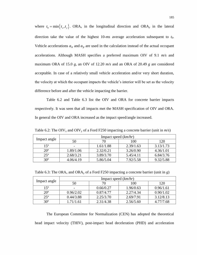
185
where 0 min , .x yt t t ORAx in the longitudinal direction and ORAy in the lateral
direction take the value of the highest 10-ms average acceleration subsequent to t0.
Vehicle accelerations and are used in the calculation instead of the actual occupant
accelerations. Although MASH specifies a preferred maximum OIV of 9.1 m/s and
maximum ORA of 15.0 g, an OIV of 12.20 m/s and an ORA of 20.49 g are considered
acceptable. In case of a relatively small vehicle acceleration and/or very short duration,
the velocity at which the occupant impacts the vehicle’s interior will be set as the velocity
difference before and after the vehicle impacting the barrier.
Table 6.2 and Table 6.3 list the OIV and ORA for concrete barrier impacts
respectively. It was seen that all impacts met the MASH specification of OIV and ORA.
In general the OIV and ORA increased as the impact speed/angle increased.
Table 6.2: The OIVx and OIVy of a Ford F250 impacting a concrete barrier (unit in m/s)
Impact angle Impact speed (km/hr)
50 70 100 120
15º - 1.61/1.88 2.39/1.63 3.13/1.73
20º 1.89/1.06 2.32/0.21 3.26/0.90 4.36/1.01
25º 2.68/3.21 3.89/3.70 5.45/4.11 6.84/3.76
30º 4.06/4.19 5.86/5.04 7.92/5.58 9.32/5.88
Table 6.3: The ORAx and ORAy of a Ford F250 impacting a concrete barrier (unit in g)
Impact angle Impact speed (km/hr)
50 70 100 120
15º - 0.66/0.27 1.96/0.63 0.96/1.61
20º 0.96/2.02 0.87/4.77 2.27/4.34 0.90/1.02
25º 0.44/3.88 2.25/3.70 2.69/7.91 3.12/8.13
30º 1.71/1.61 2.31/4.38 2.56/5.60 4.77/7.68
The European Committee for Normalization (CEN) has adopted the theoretical
head impact velocity (THIV), post-impact head deceleration (PHD) and acceleration
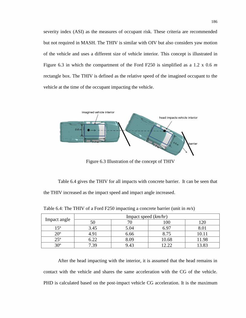
186
severity index (ASI) as the measures of occupant risk. These criteria are recommended
but not required in MASH. The THIV is similar with OIV but also considers yaw motion
of the vehicle and uses a different size of vehicle interior. This concept is illustrated in
Figure 6.3 in which the compartment of the Ford F250 is simplified as a 1.2 x 0.6 m
rectangle box. The THIV is defined as the relative speed of the imagined occupant to the
vehicle at the time of the occupant impacting the vehicle.
Figure 6.3 Illustration of the concept of THIV
Table 6.4 gives the THIV for all impacts with concrete barrier. It can be seen that
the THIV increased as the impact speed and impact angle increased.
Table 6.4: The THIV of a Ford F250 impacting a concrete barrier (unit in m/s)
Impact angle Impact speed (km/hr)
50 70 100 120
15º 3.45 5.04 6.97 8.01
20º 4.91 6.66 8.75 10.11
25º 6.22 8.09 10.68 11.98
30º 7.39 9.43 12.22 13.83
After the head impacting with the interior, it is assumed that the head remains in
contact with the vehicle and shares the same acceleration with the CG of the vehicle.
PHD is calculated based on the post-impact vehicle CG acceleration. It is the maximum

187
value of the resultant acceleration filtered by a Butterworth low-pass filter with a cut-off
frequency of 10 Hz and averaged over a moving 10-ms time period. Currently the PHD is
not used in occupant injury evaluation by either MASH or CEN. Table 6.5 lists PHD
values for all the impacts with concrete barrier.
Table 6.5: The PHD of a Ford F250 impacting a concrete barrier (unit in g)
Impact angle Impact speed (km/hr)
50 70 100 120
15º 6.49 6.33 6.98 8.00
20º 4.56 7.11 8.21 9.22
25º 5.02 6.86 10.86 11.39
30º 5.66 8.83 11.85 13.47
Just like THIV and PHD, the acceleration of vehicle CG provides the basis for
calculating ASI to evaluate the overall impact severity by a single index. ASI is defined
as
122 2 2
( )ˆ ˆ ˆ
yx z
x y z
aa aASI t
a a a
(6.7)
where ̅ , ̅ , ̅ are the 50-ms average vehicle accelerations and ̂ , ̂ , ̂ are the
threshold accelerations ( ̂ = 12 g, ̂ = 9 g and ̂ = 10 g). Normally the maximum
value of is taken as the single index ASI. The more ASI exceeds unity, the more
the risk to the occupant (CEN 1998). Although a maximum ASI value of 1.0 is
recommended, a maximum ASI value of 1.4 is acceptable. However, no details regarding
the basis for ASI threshold values are provided. Table 6.6 gives ASI values for all the
concrete barrier impacts. Generally speaking, the larger impact speed/angle, the larger
ASI was. Impact with speed of 50 km/hr and impact angle of 15° and impact with speed

188
of 120 km/hr and impact angle of 30° had the least and most severe impact index ASI
respectively.
Table 6.6: The ASI of a Ford F250 impacting a concrete barrier
Impact angle Impact speed (km/hr)
50 70 100 120
15º 0.4 0.65 1.09 1.18
20º 0.57 0.81 1.39 1.35
25º 0.73 0.99 1.6 1.99
30º 0.86 1.22 2.19 2.69
Table 6.7 lists the time instants for maximum ASI. It was noticed that maximum
ASI took place very early when the occupant had not gone through any apparent relative
motion to the vehicle interior. This observation further highlighted that ASI is an index to
evaluate vehicle impact severity but not directly estimate occupant risk. In addition,
larger impact angle tended to achieve maximum ASI even earlier.
Table 6.7: The time instants of maximum ASI in concrete barrier impacts (unit in ms)
Impact angle Impact speed (km/hr)
50 70 100 120
15º 74.00 132.16 118.40 104.08
20º 63.92 123.28 123.92 103.44
25º 60.48 129.44 31.76 23.28
30º 50.24 44.32 23.52 21.76
Using ASI and THIV together, the CEN defines three impact severity
levels/classes: A, B and C (Table 6.8), “impact severity level A affords a greater level of
safety for the occupant of an errant car than level B, and level B greater than level C”
(CEN 1998). It is generally desired to achieve a level A to ensure low injury likelihood
on the occupant.
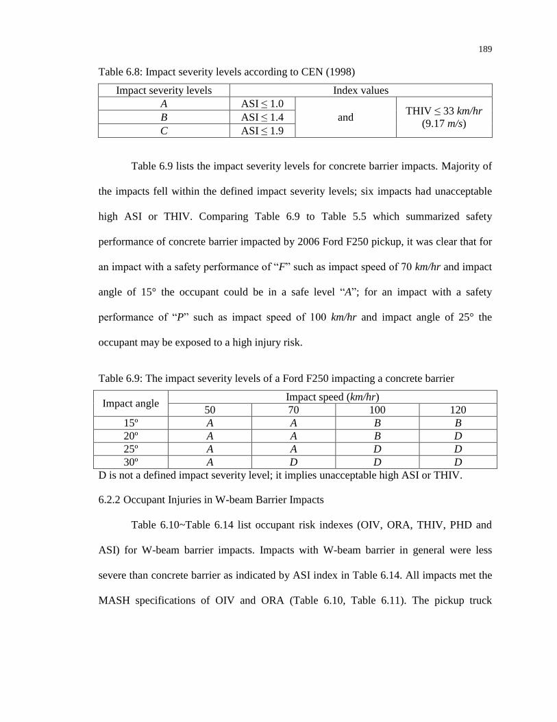
189
Table 6.8: Impact severity levels according to CEN (1998)
Impact severity levels Index values
A ASI ≤ 1.0
and THIV ≤ 33 km/hr
(9.17 m/s) B ASI ≤ 1.4
C ASI ≤ 1.9
Table 6.9 lists the impact severity levels for concrete barrier impacts. Majority of
the impacts fell within the defined impact severity levels; six impacts had unacceptable
high ASI or THIV. Comparing Table 6.9 to Table 5.5 which summarized safety
performance of concrete barrier impacted by 2006 Ford F250 pickup, it was clear that for
an impact with a safety performance of “F” such as impact speed of 70 km/hr and impact
angle of 15° the occupant could be in a safe level “A”; for an impact with a safety
performance of “P” such as impact speed of 100 km/hr and impact angle of 25° the
occupant may be exposed to a high injury risk.
Table 6.9: The impact severity levels of a Ford F250 impacting a concrete barrier
Impact angle Impact speed (km/hr)
50 70 100 120
15º A A B B
20º A A B D
25º A A D D
30º A D D D
D is not a defined impact severity level; it implies unacceptable high ASI or THIV.
6.2.2 Occupant Injuries in W-beam Barrier Impacts
Table 6.10~Table 6.14 list occupant risk indexes (OIV, ORA, THIV, PHD and
ASI) for W-beam barrier impacts. Impacts with W-beam barrier in general were less
severe than concrete barrier as indicated by ASI index in Table 6.14. All impacts met the
MASH specifications of OIV and ORA (Table 6.10, Table 6.11). The pickup truck
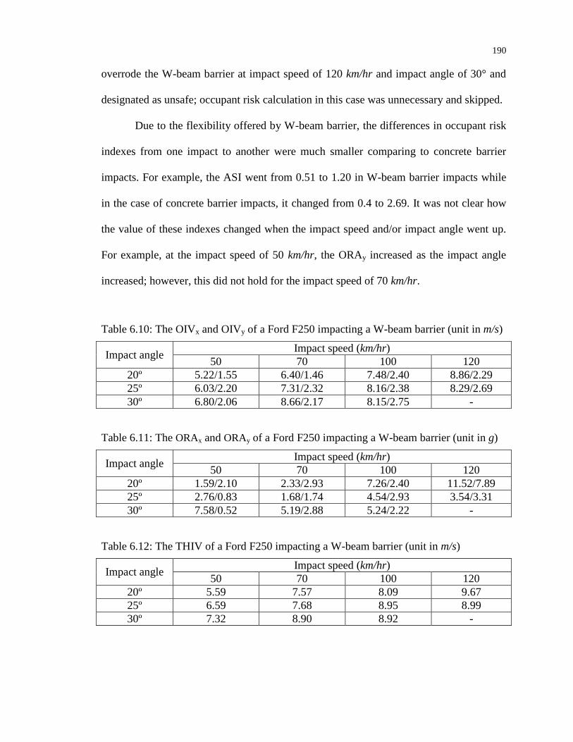
190
overrode the W-beam barrier at impact speed of 120 km/hr and impact angle of 30° and
designated as unsafe; occupant risk calculation in this case was unnecessary and skipped.
Due to the flexibility offered by W-beam barrier, the differences in occupant risk
indexes from one impact to another were much smaller comparing to concrete barrier
impacts. For example, the ASI went from 0.51 to 1.20 in W-beam barrier impacts while
in the case of concrete barrier impacts, it changed from 0.4 to 2.69. It was not clear how
the value of these indexes changed when the impact speed and/or impact angle went up.
For example, at the impact speed of 50 km/hr, the ORAy increased as the impact angle
increased; however, this did not hold for the impact speed of 70 km/hr.
Table 6.10: The OIVx and OIVy of a Ford F250 impacting a W-beam barrier (unit in m/s)
Impact angle Impact speed (km/hr)
50 70 100 120
20º 5.22/1.55 6.40/1.46 7.48/2.40 8.86/2.29
25º 6.03/2.20 7.31/2.32 8.16/2.38 8.29/2.69
30º 6.80/2.06 8.66/2.17 8.15/2.75 -
Table 6.11: The ORAx and ORAy of a Ford F250 impacting a W-beam barrier (unit in g)
Impact angle Impact speed (km/hr)
50 70 100 120
20º 1.59/2.10 2.33/2.93 7.26/2.40 11.52/7.89
25º 2.76/0.83 1.68/1.74 4.54/2.93 3.54/3.31
30º 7.58/0.52 5.19/2.88 5.24/2.22 -
Table 6.12: The THIV of a Ford F250 impacting a W-beam barrier (unit in m/s)
Impact angle Impact speed (km/hr)
50 70 100 120
20º 5.59 7.57 8.09 9.67
25º 6.59 7.68 8.95 8.99
30º 7.32 8.90 8.92 -
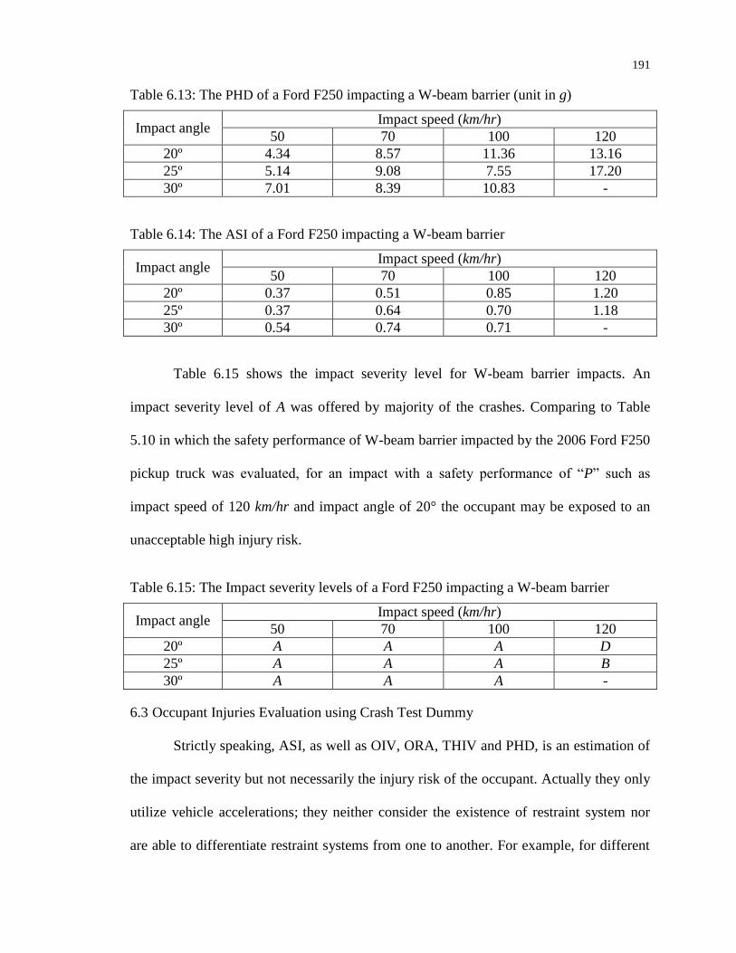
191
Table 6.13: The PHD of a Ford F250 impacting a W-beam barrier (unit in g)
Impact angle Impact speed (km/hr)
50 70 100 120
20º 4.34 8.57 11.36 13.16
25º 5.14 9.08 7.55 17.20
30º 7.01 8.39 10.83 -
Table 6.14: The ASI of a Ford F250 impacting a W-beam barrier
Impact angle Impact speed (km/hr)
50 70 100 120
20º 0.37 0.51 0.85 1.20
25º 0.37 0.64 0.70 1.18
30º 0.54 0.74 0.71 -
Table 6.15 shows the impact severity level for W-beam barrier impacts. An
impact severity level of A was offered by majority of the crashes. Comparing to Table
5.10 in which the safety performance of W-beam barrier impacted by the 2006 Ford F250
pickup truck was evaluated, for an impact with a safety performance of “P” such as
impact speed of 120 km/hr and impact angle of 20° the occupant may be exposed to an
unacceptable high injury risk.
Table 6.15: The Impact severity levels of a Ford F250 impacting a W-beam barrier
Impact angle Impact speed (km/hr)
50 70 100 120
20º A A A D
25º A A A B
30º A A A -
6.3 Occupant Injuries Evaluation using Crash Test Dummy
Strictly speaking, ASI, as well as OIV, ORA, THIV and PHD, is an estimation of
the impact severity but not necessarily the injury risk of the occupant. Actually they only
utilize vehicle accelerations; they neither consider the existence of restraint system nor
are able to differentiate restraint systems from one to another. For example, for different
192
restraint systems, the risk of occupant injury will be considered the same as long as the
ASI value is the same. This is apparently not the case.
Injury of occupant should be specified to a particular part of the body such as
head, neck, chest, pelvis, and/or legs, etc. Each part will have their own forms of injury
and their own threshold for that specific type of injury. None of these will be indicated by
injury criteria based solely on vehicle responses such as ASI, OIV, ORA, THIV and PHD.
At best they are assessments of the injury at the whole body level.
There is the discrepancy about direct and detailed knowledge of human injury in a
traffic median barrier crashes which cannot be obtained from vehicle responses only.
Researchers in crashworthiness analysis field have adopted crash test dummies in both
crash tests and simulations to study human responses. In roadside barrier crashes, due to a
few limitations the vehicular behaviors are still the only factors to be investigated and
used to evaluate the safety performance of the barrier. Occupant risk evaluation is based
on vehicle accelerations; direct injury evaluation using crash test dummy hasn’t been
possible.
It is not clear whether injury criteria used in frontal impact testing and side impact
testing could be directly adopted in roadside barrier crashes; modifications may be
necessary. It is not within the scope of this research to investigate the validity and
develop new injury criteria for roadside barrier crashes if necessary; occupant risk criteria
such as HIC15, maximum chest compression (MCC) used in frontal impact test will be
calculated for concrete barrier impacts in section 6.3.1 and for W-beam barrier impacts in
section 6.3.2.

193
6.3.1 Occupant Injuries in Concrete Barrier Impacts
Table 6.16 lists the calculated HIC15 for the occupant in concrete barrier impacts.
According to NHTSA specification that HIC15 should be less than 700, two impacts were
found to fail the threshold: (1) impact speed of 100 km/hr and impact angle of 30°; and (2)
impact speed of 120 km/hr and impact angle of 30°. While according to the HIC15 values
in Table 6.16 only two of the impacts were considered to expose the occupant to
unacceptable high injury risk, by impact severity levels (Table 6.9) five of the impacts
endangered the occupant intolerably. This inconsistence may suggest an over-
conservative injury evaluation by the impact severity levels (Table 6.8) assume that the
HIC15 of 700 is accepted as a valid head injury assessment in median barrier crashes.
Table 6.16: The HIC15 of occupant during a Ford F250 impacting a concrete barrier
Impact angle Impact speed (km/hr)
50 70 100 120
15º 6 9 150 183
20º 12 61 242 343
25º 31 173 516 661
30º 169 358 841 1529
Figure 6.17 gives the maximum chest compression for the occupant in concrete
barrier impacts. The chest compression was under safe threshold of 76 mm for every
impact.
Table 6.17: The MCC of occupant during a Ford F250 impacting a concrete barrier (unit
in mm)
Impact angle Impact speed (km/hr)
50 70 100 120
15º 3.51 5.11 8.54 10.21
20º 7.15 16.18 17.48 10.95
25º 11.95 16.37 19.5 17.01
30º 17.27 24.05 9.88 25.08
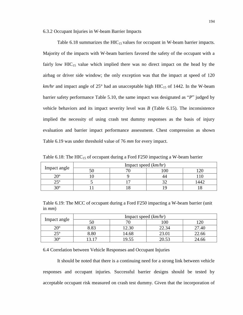
194
6.3.2 Occupant Injuries in W-beam Barrier Impacts
Table 6.18 summarizes the HIC15 values for occupant in W-beam barrier impacts.
Majority of the impacts with W-beam barriers favored the safety of the occupant with a
fairly low HIC15 value which implied there was no direct impact on the head by the
airbag or driver side window; the only exception was that the impact at speed of 120
km/hr and impact angle of 25° had an unacceptable high HIC15 of 1442. In the W-beam
barrier safety performance Table 5.10, the same impact was designated as “P” judged by
vehicle behaviors and its impact severity level was B (Table 6.15). The inconsistence
implied the necessity of using crash test dummy responses as the basis of injury
evaluation and barrier impact performance assessment. Chest compression as shown
Table 6.19 was under threshold value of 76 mm for every impact.
Table 6.18: The HIC15 of occupant during a Ford F250 impacting a W-beam barrier
Impact angle Impact speed (km/hr)
50 70 100 120
20º 10 9 44 110
25º 5 17 32 1442
30º 11 18 19 18
Table 6.19: The MCC of occupant during a Ford F250 impacting a W-beam barrier (unit
in mm)
Impact angle Impact speed (km/hr)
50 70 100 120
20º 8.83 12.30 22.34 27.40
25º 8.80 14.68 23.01 22.66
30º 13.17 19.55 20.53 24.66
6.4 Correlation between Vehicle Responses and Occupant Injuries
It should be noted that there is a continuing need for a strong link between vehicle
responses and occupant injuries. Successful barrier designs should be tested by
acceptable occupant risk measured on crash test dummy. Given that the incorporation of
195
crash test dummy is necessary but not feasible, correlation between the vehicle responses
with occupant risk if successfully constructed should greatly simplify the barrier testing
procedures and provide greater confidence to existing barrier systems. Attempts have
been tried by Ray et al. (1987) who investigated the correlation of OIV to the HIC15 with
3 frontal sled tests and to the TTI with 4 side impacts. The study indicated that the
roadside criteria may be overly conservative as a 8 m/s OIV corresponded to a mild 316
HIC15 and a relatively low TTI of 113 (16% probability of AIS 3 injury or greater). The
results led to the subsequent increase in the lateral OIV from 9 m/s to 12 m/s in NCHRP
Report 350. Council and Stewart (1993) showed a lack of strong relationship between
occupant injury and maximum longitudinal and lateral impact forces to the vehicle.
Shojaati (2003) suggested an exponential relation between HIC15 and ASI using nine
lateral sled tests. Using data from frontal impact tests, Gabauer and Thomson (2005)
showed that there was correlation between ASI and some injury criteria such as MCC.
As had been shown, an acceptable safety performance of the barrier solely based
on vehicle behaviors was not a guarantee of an acceptable occupant injury level and a
failed barrier impact performance did not necessarily lead to intolerable high injury risk.
With the injury evaluation discussed in section 6.2 and section 6.3, it was possible to use
the simulation data of the median barrier crashes to study the correlation between the
vehicle responses based injury criteria and crash test dummy based injury criteria. This
correlation if any was revealed by a curve fitting process in which the polynomial was
first tried and the simplest form was always favored. For example, with the same R-
square value 2nd
order polynomial was preferred over 6th
order polynomial; if no
appropriate polynomial form with reasonable R-square value was found then a power law

196
and/or exponential correlation was sought after. Ideally all the fitting curves should go
through the origin (0, 0). The two important injury criteria, HIC15 and MCC, were studied
regarding their potential correlation to vehicle responses based injury criteria (ASI, THIV,
PHD, OIV and ORA). Only the correlations with strongest R-square value were
presented.
6.4.1 Ford Pickup Truck Impacting Rigid Concrete Barrier
HIC15 was plotted against ASI, THIV, PHD, OIV and ORA respectively (Figure
6.4~Figure 6.7) and its correlation to ASI, THIV, PHD, OIV and ORA was shown in
Table 6.20. ASI (Figure 6.4a), THIV (Figure 6.4b) and OIVx (Figure 6.6a) all showed a
strong quadratic polynomial correlation to HIC15. On the contrary, there was lack of
strong correlation between HIC15 and other vehicle responses based injury criteria: PHD
(Figure 6.5), OIVy (Figure 6.6b) and ORA (Figure 6.7).
Table 6.20: Correlation of HIC15 with OIV, ORA, ASI, THIV and PHD
f(x) = a0x2
+ b0x + c0
f(x) = a1xk
Coefficients
a0 b0 c0 a1 k R2
HIC15
OIVx 22.21 -66.72 113.89 - - 0.96
OIVy 71.26 -281.5 340.10 - - 0.70
ORAx 72.02 -31.81 63.41 - - 0.87
ORAy 21.32 -53.51 157.71 - - 0.60
ASI 247.72 -131.8 25.22 - - 0.98
THIV - - - 0.017 4.35 0.95
PHD - - - 0.016 4.41 0.69
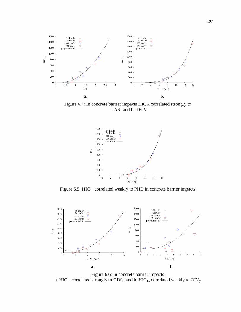
197
a. b.
Figure 6.4: In concrete barrier impacts HIC15 correlated strongly to
a. ASI and b. THIV
Figure 6.5: HIC15 correlated weakly to PHD in concrete barrier impacts
a. b.
Figure 6.6: In concrete barrier impacts
a. HIC15 correlated strongly to OIVx; and b. HIC15 correlated weakly to OIVy
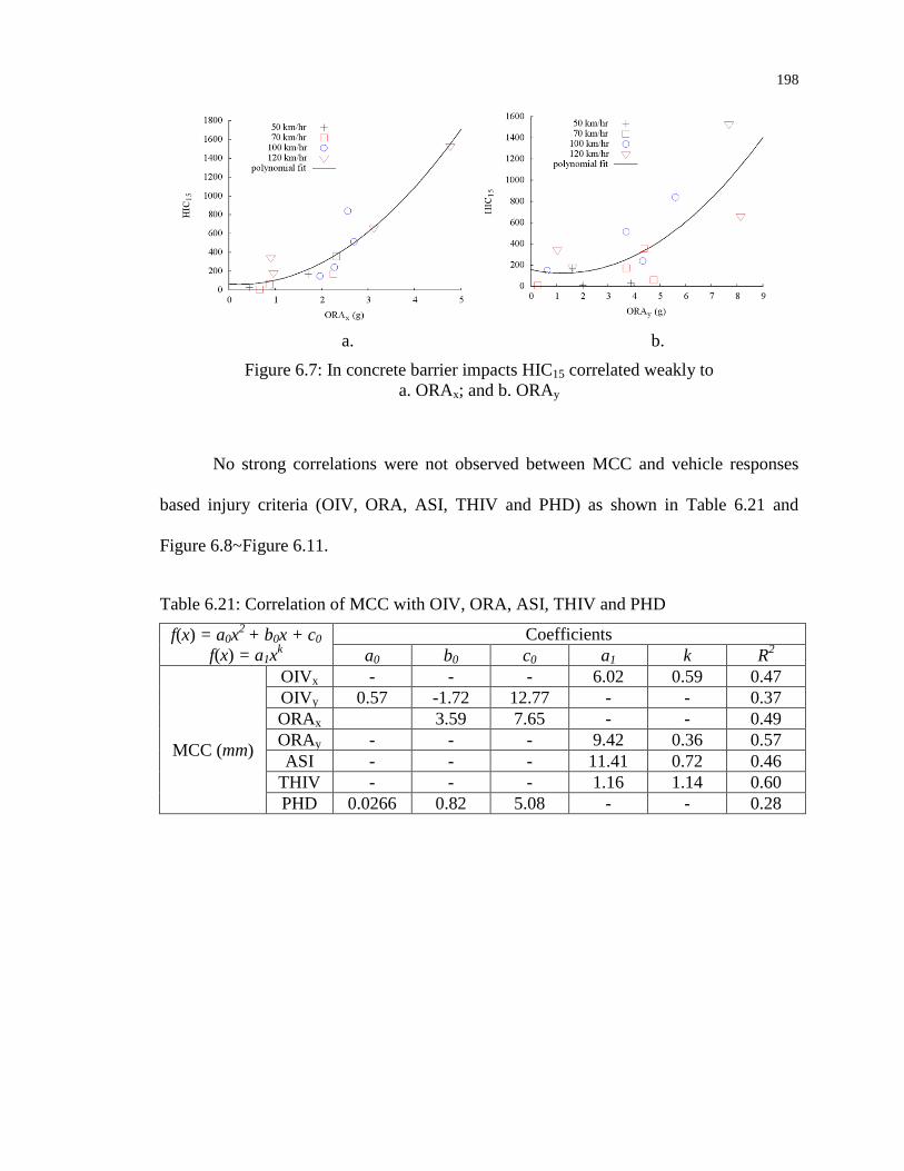
198
a. b.
Figure 6.7: In concrete barrier impacts HIC15 correlated weakly to
a. ORAx; and b. ORAy
No strong correlations were not observed between MCC and vehicle responses
based injury criteria (OIV, ORA, ASI, THIV and PHD) as shown in Table 6.21 and
Figure 6.8~Figure 6.11.
Table 6.21: Correlation of MCC with OIV, ORA, ASI, THIV and PHD
f(x) = a0x2
+ b0x + c0
f(x) = a1xk
Coefficients
a0 b0 c0 a1 k R2
MCC (mm)
OIVx - - - 6.02 0.59 0.47
OIVy 0.57 -1.72 12.77 - - 0.37
ORAx 3.59 7.65 - - 0.49
ORAy - - - 9.42 0.36 0.57
ASI - - - 11.41 0.72 0.46
THIV - - - 1.16 1.14 0.60
PHD 0.0266 0.82 5.08 - - 0.28

199
a. b.
Figure 6.8: In concrete barrier impacts MCC correlated weakly to
a. ASI and b. THIV
Figure 6.9: MCC correlated weakly to PHD in concrete barrier impacts
a. b.
Figure 6.10: In concrete barrier impacts MCC correlated weakly to
a. OIVx and b. OIVy
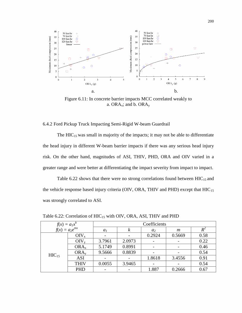
200
a. b.
Figure 6.11: In concrete barrier impacts MCC correlated weakly to
a. ORAx; and b. ORAy
6.4.2 Ford Pickup Truck Impacting Semi-Rigid W-beam Guardrail
The HIC15 was small in majority of the impacts; it may not be able to differentiate
the head injury in different W-beam barrier impacts if there was any serious head injury
risk. On the other hand, magnitudes of ASI, THIV, PHD, ORA and OIV varied in a
greater range and were better at differentiating the impact severity from impact to impact.
Table 6.22 shows that there were no strong correlations found between HIC15 and
the vehicle response based injury criteria (OIV, ORA, THIV and PHD) except that HIC15
was strongly correlated to ASI.
Table 6.22: Correlation of HIC15 with OIV, ORA, ASI, THIV and PHD
f(x) = a1xk
f(x) = a2emx
Coefficients
a1 k a2 m R2
HIC15
OIVx - - 0.2924 0.5669 0.58
OIVy 3.7961 2.0973 - - 0.22
ORAx 5.1749 0.8991 - - 0.46
ORAy 9.5666 0.8839 - - 0.54
ASI - - 1.8618 3.4556 0.91
THIV 0.0055 3.9465 - - 0.54
PHD - - 1.887 0.2666 0.67

201
Figure 6.12: HIC15 correlated strongly to ASI in W-beam barrier impacts
a. b.
Figure 6.13: In W-beam barrier impacts HIC15 correlated weakly to
a. THIV and b. PHD
a. b.
Figure 6.14: In W-beam barrier impacts HIC15 correlated weakly to
a. OIVx; and b. OIVy
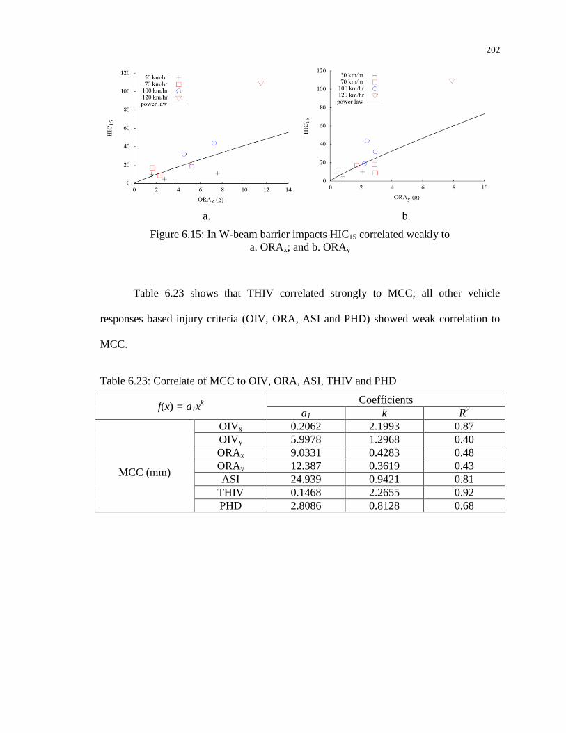
202
a. b.
Figure 6.15: In W-beam barrier impacts HIC15 correlated weakly to
a. ORAx; and b. ORAy
Table 6.23 shows that THIV correlated strongly to MCC; all other vehicle
responses based injury criteria (OIV, ORA, ASI and PHD) showed weak correlation to
MCC.
Table 6.23: Correlate of MCC to OIV, ORA, ASI, THIV and PHD
f(x) = a1xk Coefficients
a1 k R2
MCC (mm)
OIVx 0.2062 2.1993 0.87
OIVy 5.9978 1.2968 0.40
ORAx 9.0331 0.4283 0.48
ORAy 12.387 0.3619 0.43
ASI 24.939 0.9421 0.81
THIV 0.1468 2.2655 0.92
PHD 2.8086 0.8128 0.68
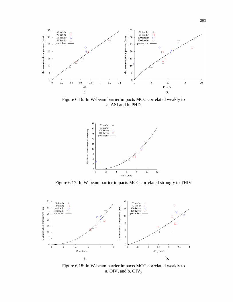
203
a. b.
Figure 6.16: In W-beam barrier impacts MCC correlated weakly to
a. ASI and b. PHD
Figure 6.17: In W-beam barrier impacts MCC correlated strongly to THIV
a. b.
Figure 6.18: In W-beam barrier impacts MCC correlated weakly to
a. OIVx and b. OIVy

204
a. b.
Figure 6.19: In W-beam barrier impacts MCC correlated weakly to
a. ORAx and b. ORAy
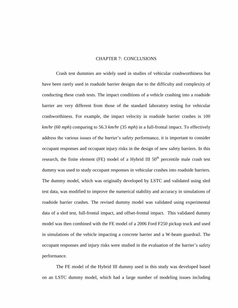
CHAPTER 7: CONCLUSIONS
Crash test dummies are widely used in studies of vehicular crashworthiness but
have been rarely used in roadside barrier designs due to the difficulty and complexity of
conducting these crash tests. The impact conditions of a vehicle crashing into a roadside
barrier are very different from those of the standard laboratory testing for vehicular
crashworthiness. For example, the impact velocity in roadside barrier crashes is 100
km/hr (60 mph) comparing to 56.3 km/hr (35 mph) in a full-frontal impact. To effectively
address the various issues of the barrier’s safety performance, it is important to consider
occupant responses and occupant injury risks in the design of new safety barriers. In this
research, the finite element (FE) model of a Hybrid III 50th
percentile male crash test
dummy was used to study occupant responses in vehicular crashes into roadside barriers.
The dummy model, which was originally developed by LSTC and validated using sled
test data, was modified to improve the numerical stability and accuracy in simulations of
roadside barrier crashes. The revised dummy model was validated using experimental
data of a sled test, full-frontal impact, and offset-frontal impact. This validated dummy
model was then combined with the FE model of a 2006 Ford F250 pickup truck and used
in simulations of the vehicle impacting a concrete barrier and a W-beam guardrail. The
occupant responses and injury risks were studied in the evaluation of the barrier’s safety
performance.
The FE model of the Hybrid III dummy used in this study was developed based
on an LSTC dummy model, which had a large number of modeling issues including
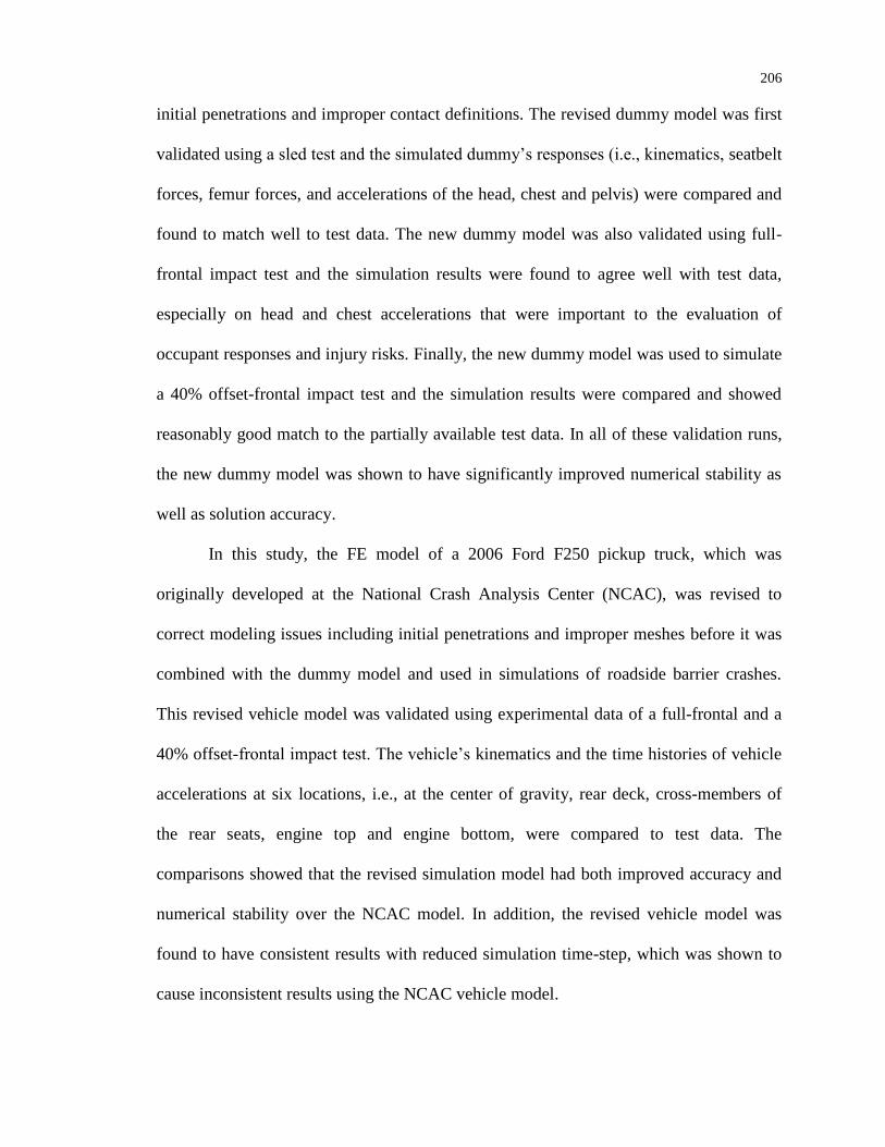
206
initial penetrations and improper contact definitions. The revised dummy model was first
validated using a sled test and the simulated dummy’s responses (i.e., kinematics, seatbelt
forces, femur forces, and accelerations of the head, chest and pelvis) were compared and
found to match well to test data. The new dummy model was also validated using full-
frontal impact test and the simulation results were found to agree well with test data,
especially on head and chest accelerations that were important to the evaluation of
occupant responses and injury risks. Finally, the new dummy model was used to simulate
a 40% offset-frontal impact test and the simulation results were compared and showed
reasonably good match to the partially available test data. In all of these validation runs,
the new dummy model was shown to have significantly improved numerical stability as
well as solution accuracy.
In this study, the FE model of a 2006 Ford F250 pickup truck, which was
originally developed at the National Crash Analysis Center (NCAC), was revised to
correct modeling issues including initial penetrations and improper meshes before it was
combined with the dummy model and used in simulations of roadside barrier crashes.
This revised vehicle model was validated using experimental data of a full-frontal and a
40% offset-frontal impact test. The vehicle’s kinematics and the time histories of vehicle
accelerations at six locations, i.e., at the center of gravity, rear deck, cross-members of
the rear seats, engine top and engine bottom, were compared to test data. The
comparisons showed that the revised simulation model had both improved accuracy and
numerical stability over the NCAC model. In addition, the revised vehicle model was
found to have consistent results with reduced simulation time-step, which was shown to
cause inconsistent results using the NCAC vehicle model.
207
Occupant responses in roadside barrier crashes were studied in this research using
numerical simulations with the revised FE models of the Hybrid III dummy and the 2006
Ford F250 equipped with an airbag and a seatbelt system. The crash simulations were
performed on two longitudinal barrier systems: a New Jersey concrete barrier and a
standard G4 (1s) W-beam guardrail. The impact conditions used in these simulations
were based on the standard Test Level 3 (TL-3) conditions specified by the Manual for
Assessing Safety Hardware (MASH) for longitudinal barriers. The TL-3 conditions
include vehicular impacts of a 1291-kg (2846-lb) small passenger car and a 2979-kg
(6567-lb) pickup truck. For the pickup truck impact, the MASH TL-3 conditions specify
an impact speed of 100 km/hr (62 mph) and a 25 impact angle. In addition to the
standard TL-3 conditions, crash simulations were also performed at an impact speed of
100 km/hr (62 mph) and impact angles of 15, 20 and 30, and at an impact speed of 120
km/hr (75 mph) and a 25 impact angle. Both the vehicular and occupant responses were
extracted from the simulation results to evaluate the severity of occupant injuries.
Traditional criteria on occupant injury, such as the occupant impact velocity
(OIV), occupant ridedown acceleration (ORA), theoretical head impact velocity (THIV),
post-impact head deceleration (PHD) and acceleration severity index (ASI), were
obtained based on the vehicle’s acceleration histories for impacts on both the concrete
barrier and W-beam guardrail. These criteria were compared to the head injury criteria
(HIC) and maximum chest compression (MCC) that were calculated using occupant
responses. The comparisons showed that the occupant injury criteria solely based on
vehicular responses, e.g., the OIV, were insufficient to evaluate the occupant injury risk.
The simulation results of the Ford F250 impacting the concrete barrier and W-beam

208
guardrail showed that a crash with an OIV below the MASH threshold value could have
an unacceptably high HIC15 value. This indicated that an accurate assessment of occupant
injury should be based on occupant responses in addition to vehicular responses.
For vehicular crashes into the rigid concrete barrier, the simulation showed that
some injury criteria based on vehicular responses such as the OIV, THIV and ASI
correlate strongly with occupant injuries and could be reliably used to indicate the
relative level of occupant injury, although a specific value would not give a clear
indication of the actual injury level. For vehicular crashes into the semi-rigid W-beam
guardrail, the correlation between vehicular responses and occupant injury was found not
as strong as that observed in the case of the concrete barrier. The reasons were that the
W-beam guardrail had more severe deformation and thus more interactions with the
vehicle than the concrete barrier, resulting in generally small HIC15. This indicated that,
for W-beam guardrails, the injury criteria solely based on vehicular responses might not
give reliable indications of the occupant injury even on the relative injury levels.
Therefore, injury criteria based on occupant responses, such as the HIC15, should be
adopted to obtain more accurate assessment of occupant injuries and the performances of
the barrier.
This research clearly demonstrated the usefulness and promise of finite element
modeling and simulation in roadside safety research. Given the complexity and
challenges involved in roadside hardware designs, there is much to be done to improve
the modeling capability and simulation accuracy. The simulation models used in this
research, i.e., the Hybrid III dummy and pickup truck models, could be further improved
and used to study other crash scenarios and roadside barriers.
209
REFERENCES
Arnoux, P. J., Joonekindt, S., Thollon, L. and Kayvantash, K. (2003). "Radioss Finite
Element Model of The Thor Dummy." International Journal of Crashworthiness
8(6): 529-541.
Atahan, A. O. (2010). "Vehicle Crash Test Simulation of Roadside Hardware Using LS-
DYNA: A Literature Review." International Journal of heavy vehicle systems
17(1): 52-75.
Avula, X. J. R., Kaleps, I. and Mysore, P. (1998). Forces And Deformed Configuration of
An Airbag During Inflation And Impact. Rto Meeting Proceedings 20 Models for
Aircrew Safety Assessment - Uses, Limitations and Requirements, Ohio, USA.
Avula, X. J. R., Kaleps, I. and Mysore, P. (1999). Nonlinear Finite Element Modeling of
an Airbag During Inflation and Impact.
Backaitis, S. and Mertz, H. (1994). Hybrid III: The First Human-Like Crash Test Dummy,
Society of Automotive Engineers.
Bathe, K.-J. (2001). "The inf–sup condition and its evaluation for mixed finite element
methods." Computers & Structures 79(2): 243-252.
Behr, M., Arnoux, P. J., Serre, T., Bidal, S., Kang, H. S., Thollon, L., Cavallero, C.,
Kayvantash, K. and Brunet, C. (2003). "A Human Model for Road Safety: From
Geometrical Acquisition to Model Validation with Radioss." Computer Methods
in Biomechanics and Biomedical Engineering 6(4): 263-273.
Benson, D. J. and Hallquist, J. O. (1990). "A Single Surface Contact Algorithm for The
Post-buckling Analysis of Shell Structures." Computer Methods in Applied
Mechanics and Engineering 78(2): 141-163.
Boesch, D. A. and Reid, J. D. (2005). Further Improvements to The Truck Model for
Roadside Safety Simulation - Suspension and Steering. the 5th European LS-
DYNA Users Conference. Birmingham, UK.
Burton, D. E., Lettis, L. A. J., Bryan, J. B. and Frary, N. R. (1982). Physics and Numerics
of the Tensor Code (Incomplete Preliminary Documentation): Medium: ED; Size:
Pages: 91.
CEN (1998). "Road Restraint Systems – Part 2: Performance Classes, Impact Test
Acceptance Criteria and Test Methods for Safety Barriers." European Standard
EN 1317-2.
Chaudhary, A. B. and Bathe, K. J. (1985). A Lagrange Multiplier Segment Procedure for
Solution of Three Dimensional Contact Problems, US Army Ballistic Research
Laboratory: 76.

210
Cheng, Z. Q., Thacker, J. G., Pilkey, W. D., Hollowell, W. T., Reagan, S. W. and Sieveka,
E. M. (2001). "Experiences in Reverse-engineering of A Finite Element
Automobile Crash Model." Finite Elements in Analysis and Design 37(11): 843-
860.
Chou, C. C., McCoy, R. W. and Le, J. (2005). "A Literature Review of Rollover Test
Methodologies." International Journal of Vehicle Safety 1(1): 200-237.
Consolazio, G. R., Chung, J. H. and Gurley, K. R. (2003). "Impact Simulation and Full
Scale Crash Testing of A Low Profile Concrete Work Zone Barrier." Computers
& Structures 81(13): 1359-1374.
Council, F. M. and Stewart, J. R. (1993). "Attempt to Define Relationship Between
Forces to Crash-test Vehicles and Occupant Injury in Similar Real-world
Crashes." Transportation Research Record: 78-78.
Crisfield, M. A. (2000). "Re-visiting The Contact Patch Test." International Journal for
Numerical Methods in Engineering 48(3): 435-449.
Culver, C. C., Neathery, R. F. and Mertz, H. J. (1972). "Mechanical Necks with
Humanlike Responses." SAE Technical Paper 720959.
De Lorenzis, L., Temizer, İ., Wriggers, P. and Zavarise, G. (2011). "A Large
Deformation Frictional Contact Formulation Using NURBS-based Isogeometric
Analysis." International Journal for Numerical Methods in Engineering 87(13):
1278-1300.
Dubois, D., Gross, P., Trameçon, A. and Markiewicz, E. (2006). "Finite Element
Analysis of Seat Belt Bunching Phenomena." International Journal of
Crashworthiness 11(6): 519-528.
Dubois, D., Silverthorne, P. and Markiewicz, E. (2011). "Assessment of Seat Belt
Webbing Bunching Phenomena." International Journal of Impact Engineering
38(5): 339-357.
Dubois, D., Zellmer, H. and Markiewicz, E. (2009). "Experimental and Numerical
Analysis of Seat Belt Bunching Phenomenon." International Journal of Impact
Engineering 36(6): 763-774.
El-Abbasi, N. and Bathe, K.-J. (2001). "Stability And Patch Test Performance of Contact
Discretizations And A New Solution Algorithm." Computers & Structures
79(16): 1473-1486.
Ennis, J. B., Marzougui, D., Eskandarian, A. and Bedewi, N. E. (2001). "Finite Element
Modelling of Anthropomorphic Test Devices for Vehicle Crashworthiness
Evaluation." International Journal of Crashworthiness 6(4): 511-524.
211
Eppinger, R., Sun, E., Bandak, F., Haffner, M., Khaewpong, N., Maltese, M., Kuppa, S.,
Nguyen, T., Takhounts, E., Tannous, R., Zhang, A. and Saul, R. (1999).
"Development of Improved Injury Criteria for The Assessment of Advanced
Automotive Restraint Systems–II." National Highway Traffic Safety
Administration: 1-70.
Eppinger, R. H., Marcus, J. H. and Morgan, R. M. (1984). "Development of Dummy and
Injury index for NHTSA's Thoracic Side Impact Protection Research Program."
SAE Technical Paper 840885.
Foster, J. K., Kortge, J. O. and Wolanin, M. J. (1977). "Hybrid III-A Biomechanically-
Based Crash Test Dummy." SAE Technical Paper 770938.
Franke, D., Düster, A., Nübel, V. and Rank, E. (2010). "A Comparison of The h-, p-, hp-,
And rp-version of The FEM for The Solution of The 2D Hertzian Contact
Problem." Computational Mechanics 45(5): 513-522.
Franz, U. and Graf, O. (2000). Accurate and Detailed LS-DYNA FE Models of the US-
and EUROSID: A Review of the German FAT Project 6th International LS-
DYNA Conference. USA.
Franz, U., Schuster, P., Schmid, W. and Graf, O. (2003). FAT Side Impact Dummy
Models–Remarks on Usage and Potential Pitfalls. 4th European LS-DYNA Users
Conference, Ulm, Germany.
Franz, U., Walz, M. and Graf, O. (1999). Enhancements to the FAT FE Dummies Using
Specific Features of LS-DYNA. 2nd European LS-DYNA Conference,
Gothenburg, Sweden.
Gabauer, D. and Thomson, R. (2005). Correlation of Vehicle and Roadside Crash Test
Injury Criteria. 19th International Technical Conference on the Enhanced Safety
of Vehicles (ESV)-Washington DC June.
Gayzik, F. S., Moreno, D. P., Vavalle, N. A., Rhyne, A. C. and Stitzel, J. D. (2012).
Development of a Full Human Body Finite Element Model for Blunt Injury
Prediction Utilizing a Multi-Modality Medical Imaging Protocol. the 12th
International LS-DYNA Users Conference, Detroit, USA.
Gehre, C., Taylak, E., Oancea, V., Stahlschmidt, S., Gromer, A., Berger, A. and Thibaud,
C. (2009). Development of a Computational Model of the World SID 50th Male,
National Highway Traffic Safety Administration (NHTSA).
Ghoreishy, M. H. R. (2008). "A State of the Art Review of the Finite Element Modelling
of Rolling Tyres." Iranian Polymer Journal 17(8): 571-597.
Gromer, A., Stahlschmidt, S. and D'Souza, R. (2009). Development of the PDB
WorldSID 50th Model for the German Automotive Industry. 7th European LS-
DYNA Conference, Salzburg, Austria.

212
Hallquist, J. O. (1978). Numerical Treatment of Sliding Interfaces and Impact.
Hallquist, J. O. (2006). LS-DYNA® Theory Manual, Livermore Software Technology
Corporation.
Hallquist, J. O., Goudreau, G. L. and Benson, D. J. (1985). "Sliding Interfaces with
Contact-Impact in Large-scale Lagrangian Computations." Computer Methods in
Applied Mechanics and Engineering 51(1–3): 107-137.
Heinstein, M. W., Mello, F. J., Attaway, S. W. and Laursen, T. A. (2000). "Contact-
impact Modeling in Explicit Transient Dynamics." Computer Methods in Applied
Mechanics and Engineering 187(3–4): 621-640.
Hendricks, B. F., Martin, O. S. and Wekezer, J. W. (1996). Impact Simulation of the
820C Vehicle with the G2 Guardrail.
Hertz (1993). A Note on the Head Injury Criteria (HIC) as a Predictor of the Risk of
Skull Fracture. The 37th Annual Proceedings of the Association for the
Advancement of Automotive Medicine.
Hild, P. (2000). "Numerical Implementation of Two Nonconforming Finite Element
Methods for Unilateral Contact." Computer Methods in Applied Mechanics and
Engineering 184(1): 99-123.
Horsch, J. D., Melvin, J. W., Viano, D. C. and Mertz, H. J. (1991). "Thoracic Injury
Assessment of Belt Restraint Systems Based on Hybrid III Chest Compression."
SAE Technical Paper 912895.
Horsch, J. D. and Schneider, D. (1988). "Biofidelity of the Hybrid III Thorax in High-
Velocity Frontal Impact." SAE Technical Paper 880718.
Hughes, T. J. R., Cottrell, J. A. and Bazilevs, Y. (2005). "Isogeometric Analysis: CAD,
Finite elements, NURBS, Exact Geometry and Mesh Refinement." Computer
Methods in Applied Mechanics and Engineering 194(39–41): 4135-4195.
Hughes, T. J. R., Taylor, R. L., Sackman, J. L., Curnier, A. and Kanoknukulchai, W.
(1976). "A Finite Element Method for a Class of Contact-impact Problems."
Computer Methods in Applied Mechanics and Engineering 8(3): 249-276.
Iwamoto, M., Omori, K., Kimpara, H., Nakahira, Y., Tamura, A., Watanabe, I., Miki, K.,
Hasegawa, J. and Oshita, F. (2003). Recent Advances in THUMS: Development
of Individual Internal Organs, Brain, Small Female and Pedestrian Model.
Proceedings of 4th European LS-DYNA Users Conference, Ulm, Germany.
Kan, C.-D., Marzougui, D., Bahouth, G. T. and Bedewi, N. E. (2001). "Crashworthiness
Evaluation Using Integrated Vehicle and Occupant Finite Element Models."
International Journal of Crashworthiness 6(3): 387-398.
213
Khalil, T. B. and Lin, K.-H. (1991). "Hybrid III Thoracic Impact on Self-Aligning
Steering Wheel by Finite Element Analysis and Mini-Sled Experiment." SAE
Technical Paper 912894.
Khalil, T. B. and Lin, T. C. (1994). "Simulation of the Hybrid III Dummy Response to
Impact by Nonlinear Finite Element Analysis." S.A.E. transactions 103(6): 1868-
1886.
Khalil, T. B. and Sheh, M. Y. (1997). Vehicle Crashworthiness and Occupant Protection
in Frontal Impact by FE Analysis — An Integrated Approach. Crashworthiness of
Transportation Systems: Structural Impact and Occupant Protection. J. C.
Ambrósio, M. O. S. Pereira and F. Silva, Springer Netherlands. 332: 363-399.
Kikuchi, N. (1982). "A Smoothing Technique for Reduced Integration Penalty Methods
in Contact Problems." International Journal for Numerical Methods in
Engineering 18(3): 343-350.
Kikuchi, N. and Oden, J. T. (1988). Contact Problems in Elasticity: A Study of
Variational Inequalities and Finite Element Methods, SIAM.
Kim, J.-Y. and Youn, S.-K. (2012). "Isogeometric Contact Analysis Using Mortar
Method." International Journal for Numerical Methods in Engineering 89(12):
1559-1581.
King, A. I. (2000). "Fundamentals of Impact Biomechanics: Part I - Biomechanics of the
Head, Neck, and Thorax " Annual Review of Biomedical Engineering 2(1): 55-81.
King, A. I. (2001). "Fundametals of Impact Biomechanics: Part 2 - Biomechanics of the
Abdomen, Pelvis, and Lower Extremities." Annual Review of Biomedical
Engineering 3(1): 27-55.
Kirkpatrick, S. W. (2000). "Development and Validation of High Fidelity Vehicle Crash
Simulation Models." SAE Transactions 109(9): 872-881.
Kleinberger, M., Sun, E., Eppinger, R., Kuppa, S. and Saul, R. (1998). Development of
Improved Injury Criteria for the Assessment of Advanced Automotive Restraint
Systems, National Highway Traffic Safety Administration Washington, DC.
Konyukhov, A. and Schweizerhof, K. (2008). "On the Solvability of Closest Point
Projection Procedures in Contact Analysis: Analysis and Solution Strategy for
Surfaces of Arbitrary Geometry." Computer Methods in Applied Mechanics and
Engineering 197(33–40): 3045-3056.
Krone, R. and Schuster, P. (2006). "An Investigation on the Importance of Material
Anisotropy in Finite-Element Modeling of the Human Femur." SAE International,
Paper Number 2006-01-0064.
214
Laursen, T. A. (2002). Computational Contact and Impact Mechanics : Fundamentals of
Modeling Interfacial Phenomena in Nonlinear Finite Element Analysis. Berlin,
Springer.
Laursen, T. A., Puso, M. A. and Sanders, J. (2012). "Mortar Contact Formulations for
Deformable-deformable Contact: Past Contributions and New Extensions for
Enriched and Embedded Interface Formulations." Computer Methods in Applied
Mechanics and Engineering 205–208(0): 3-15.
LSTC (2012). LS-DYNA® Keyword User's Manual Volume I (Version 971 R6.0.0),
Livermore Software Technology Corporation.
Lu, J. (2011). "Isogeometric Contact Analysis: Geometric Basis and Formulation for
Frictionless Contact." Computer Methods in Applied Mechanics and Engineering
200(5–8): 726-741.
Maenchen, G. and Sack, S. (1963). The TENSOR Code, California. Univ. and Livermore.
Lawrence Radiation Lab.: 1-34.
Marzougui, D., Kan, C.-D. S. and Opiela, K. S. (2010). Comparison of the Crash Test
and Simulation of an Angle Impact of a 2007 Chevrolet Silverado Pick-Up Truck
into a New Jersey-Shaped Concrete Barrier for MASH Conditions, The National
Crash Analysis Center, The George Washington University.
Marzougui, D., Kan, C.-D. S., Zink, M., Zaouk, A. and Bedewi, N. (2003). Development
and Validation of a Pick-Up Truck Suspension Finite Element Model for Use in
Crash Simulation. The National Crash Analysis Center, The George Washington
University, Report NCAC 2003-W-003.
Marzougui, D., Zink, M., Zaouk, A., Kan, C.-D. S. and Bedewi, N. (2004).
"Development and Validation of a Vehicle Suspension Finite Element Model for
Use in Crash Simulations." International Journal of Crashworthiness 9(6): 565-
576.
McDevitt, T. W. and Laursen, T. A. (2000). "A Mortar-finite Element Formulation for
Frictional Contact Problems." International Journal for Numerical Methods in
Engineering 48(10): 1525-1547.
Mertz, H. J. (1985). "Biofidelity of the Hybrid III Head." SAE Technical Paper 851245.
Mertz, H. J., Hodgson, V. R., Thomas, L. M. and Nyquist, G. W. (1978). "An
Assessment of Compressive Neck Loads Under Injury-Producing Conditions."
Physician and Sports Medicine 6(11): 95-106.
Mertz, H. J., Horsch, J. D., Horn, G. and Lowne, R. W. (1991). "Hybrid III Sternal
Deflection Associated with Thoracic Injury Severities of Occupants Restrained
with Force-Limiting Shoulder Belts." SAE Technical Paper 910812.
215
Mertz, H. J. and Patrick, L. M. (1971). "Strength and Response of the Human Neck."
Proceedings of the Fifteenth Stapp Car Crash Conference, SAE Paprt No. 710855.
Michie, J. D. (1981). "Collision Risk Assessment Based on Occupant Flail-space Model."
Transportation Research Record(796).
Mohan, P., Marzougui, D., Arispe, E. and Story, C. (2009a). Component and Full-Scale
Tests of the 2007 Chevrolet Silverado Suspension System, National Crash
Analysis Center, The George Washington University.
Mohan, P., Marzougui, D., Bedewi, N. and Meczkowski, L. (2004). Finite Element
Modeling and Validation of a 3-Strand Cable Guardrail System, National Crash
Analysis Center, The George Washington University.
Mohan, P., Marzougui, D. and Kan, C.-D. (2009b). "Development and Validation of
Hybrid III Crash Test Dummy." SAE Technical Paper 2009-01-0473.
Mohan, P., Marzougui, D. and Kan, C.-D. S. (2003). Validation of a Single Unit Truck
Model for Roadside Hardware Impacts, National Crash Analysis Center, The
George Washington University.
Mohan, P., Marzougui, D., Velde, R. V. D. and Kan, C.-D. S. (2007). Development of
Detailed Finite Element Dummy Models. LS-DYNA Anwenderforum.
Frankenthal.
Mohan, P., Park, C.-K., Marzougui, D., Kan, C.-D., Guha, S., Maurath, C. and Bhalsod,
D. (2010). LSTC/NCAC Dummy Model Development. The 11th International
LS-DYNA Users Conference, Detroit, USA.
Mohan, P., Ritter, M., Marzougui, D., Brown, D., Kan, C.-D. S. and Opiela, K. (2009c).
Modeling, Testing, and Validation of the 2007 Chevy Silverado Finite Element
Model, The National Crash Analysis Center, The George Washington University.
Nawrocki, A. and Labrosse, M. (2000). "A Finite Element Model for Simple Straight
Wire Rope Strands." Computers & Structures 77(4): 345-359.
NHTSA (1998). "Federal Motor Vehicle Safety Standards: Occupant Crash Protection.
49 C.F.R., Part 571.208.".
NHTSA (2007). Federal Motor Vehicle Safety Standards: Side Impact Protection. 49
C.F.R., Part 571.214.
NHTSA (2009). Federal Motor Vehicle Safety Standards No. 216: Roof Crush
Resistance.
NHTSA (2013). Traffic Safety Facts 2011, the National Highway Traffic Safety
Administration: 232.

216
Nordlin, E. F., Stoker, J. R. and Stoughton, R. L. (1976). "Dynamic Tests of Metal Beam
Guardrail." Transportation Research Record(66): 44-55.
Noureddine, A., Eskandarian, A. and Digges, K. (2002). "Computer Modeling and
Validation of a Hybrid III Dummy for Crashworthiness Simulation."
Mathematical and Computer Modelling 35(7–8): 885-893.
Nyquist, G. W., Begman, P. C., King, A. I. and Mertz, H. (1980). "Correlation of Field
Injuries and GM Hybrid III Dummy Responses for Lap-shoulder Belt Restraint."
Journal of biomechanical engineering 102(2): 103.
Opiela, K., Kan, S. and Marzougui, D. (2007a). Development & Validation of a 1994
Chevrolet C2500 Pick-up Truck FE Model, the National Crash Analysis Center
(NCAC) of the George Washington University(GWU).
Opiela, K., Kan, S. and Marzougui, D. (2007b). Development & Validation of a Finite
Element Model for the 1996 Dodge Neon Passenger Sedan, the National Crash
Analysis Center (NCAC) of the George Washington University(GWU).
Opiela, K., Kan, S. and Marzougui, D. (2007c). Development & Validation of a Finite
Element Model for the 1997 Geo Metro Passenger Sedan, the National Crash
Analysis Center (NCAC) of the George Washington University(GWU).
Opiela, K., Kan, S. and Marzougui, D. (2007d). Development of a Finite Element Model
for W-Beam Guardrails, the National Crash Analysis Center (NCAC) of the
George Washington University(GWU).
Opiela, K., Kan, S. and Marzougui, D. (2008a). Development & Validation of a Finite
Element Model for the 2002 Ford Explorer, the National Crash Analysis Center
(NCAC) of the George Washington University(GWU).
Opiela, K., Kan, S. and Marzougui, D. (2008b). Development & Validation of a Finite
Element Model for the 2006 Ford F250 Pickup Truck, the National Crash
Analysis Center (NCAC) of the George Washington University(GWU).
Opiela, K., Kan, S. and Marzougui, D. (2009). Development & Initial Validation of a
2007 Chevrolet Silverado Finite Element Model, the National Crash Analysis
Center (NCAC) of the George Washington University(GWU).
Opiela, K., Kan, S. and Marzougui, D. (2011). Development & Validation of a Finite
Element Model for the 2010 Toyota Yaris Passenger Sedan, the National Crash
Analysis Center (NCAC) of the George Washington University(GWU).
Orengo, F., Ray, M. H. and Plaxico, C. A. (2003). "Modeling Tire Blow-Out in Roadside
Hardware Simulations Using LS-DYNA." ASME Conference Proceedings
2003(37300): 71-80.
217
Oshita, F., Omori, K., Nakahira, Y. and Miki, K. (2002). Development of a Finite
Element Model of the Human Body. Proceedings of the 7th International LS-
DYNA Users Conference, Detroit, US.
Papadopoulos, P. and Taylor, R. L. (1992). "A Mixed Formulation for the Finite Element
Solution of Contact Problems." Computer Methods in Applied Mechanics and
Engineering 94(3): 373-389.
Pedrazzi, C., Elsäßer, K. and Schaub, S. (2001). Aspects of Seat Belt Material Simulation.
Third European LS-DYNA conference. Dynalis, Paris.
Pietrzak, G. and Curnier, A. (1999). "Large Deformation Frictional Contact Mechanics:
Continuum Formulation and Augmented Lagrangian Treatment." Computer
Methods in Applied Mechanics and Engineering 177(3–4): 351-381.
Puso, M. A. and Laursen, T. A. (2004a). "A Mortar Segment-to-segment Contact Method
for Large Deformation Solid Mechanics." Computer Methods in Applied
Mechanics and Engineering 193(6–8): 601-629.
Puso, M. A. and Laursen, T. A. (2004b). "A Mortar Segment-to-segment Frictional
Contact Method for Large Deformations." Computer Methods in Applied
Mechanics and Engineering 193(45–47): 4891-4913.
Puso, M. A., Laursen, T. A. and Solberg, J. (2008). "A Segment-to-segment Mortar
Contact Method for Quadratic Elements and Large Deformations." Computer
Methods in Applied Mechanics and Engineering 197(6–8): 555-566.
Ray, M., Plaxico, C. and Engstrand, K. (2001). "Performance of W-Beam Splices."
Transportation Research Record: Journal of the Transportation Research Board
1743(-1): 120-125.
Ray, M. H. and McGinnis, R. G. (1997). Guardrail and Median Barrier Crashworthiness,
National Academy Press.
Ray, M. H., Stutts, J. S., Hunter, W. W. and Michie, J. D. (1987). Evaluation of Design
Analysis Procedures and Acceptance Criteria for Roadside Hardware. Volume IV
- the Importance of the Occupant Risk Criteria. Final Report.
Reid, J. D., Boesch, D. A. and Bielenberg, R. W. (2007). "Detailed Tire Modeling for
Crash Applications." International Journal of Crashworthiness 12(5): 521-529.
Reid, J. D. and Coon, B. A. (2002). Finite Element Modeling of Cable Hook Bolts. the
7th International LS-DYNA User Conference, Dearborn, MI.
Reid, J. D., Lechtenberg, K. A. and Stolle, C. S. (2010). Development of Advanced Finite
Element Material Models for Cable Barrier Wire Rope. Lincoln, Nebraska,
Nebraska Transportation Center, University of Nebraska-Lincoln.
218
Reid, J. D. and Marzougui, D. (2002). "Improved Truck Model for Roadside Safety
Simulations: Part I—Structural Modeling." Transportation Research Board 1797:
53-62.
Ross, H. E., JR., D. L. S., Zimmer, R. A. and Michie, J. D. (1993). National Cooperative
Highway Research Program Report 350: Recommended Procedures for the Safety
Performance Evaluation of Highway Features. Washington, D.C., Transportation
Research Board.
Schelkle, E. and Remensperger, R. (1991a). "Integrated Occupant-Car Crash Simulation
with the Finite Element Method: The Porsche Hybrid III-Dummy and Airbag
Model." SAE Technical Paper 910654.
Schelkle, E. and Remensperger, R. (1991b). Integrated Occupant-Car Crash Simulation
With The Finite Element Method: The Porsche Hybrid Iii-Dummy And Airbag
Model. Frontal Crash Safety Technologies For The 90's.
Shams, T., Rangarajan, N., McDonald, J., Wang, Y., Platten, G., Spade, C., Pope, P. and
Haffner, M. (2005). Development of THOR-NT: Enhancement of THOR Alpha-
the NHTSA Advanced Frontal Dummy.
Shojaati, M. (2003). "Correlation between Injury Risk and Impact Severity Index ASI."
ETH Zurich.
Sicking, D. L., Mak, K. K., Rohde, J. R. and Reid, J. D. (2009). Manual for Assessing
Safety Hardware. Washington, DC, American Association of State Highway and
Transportation Officials.
Simo, J. C. and Laursen, T. A. (1992). "An Augmented Lagrangian Treatment of Contact
Problems Involving Friction." Computers & Structures 42(1): 97-116.
Simo, J. C., Wriggers, P. and Taylor, R. L. (1985). "A Perturbed Lagrangian Formulation
for the Finite Element Solution of Contact Problems." Computer Methods in
Applied Mechanics and Engineering 50(2): 163-180.
Slaats, P. M. A. (1990). Numerical Modelling of the Hybrid III Dummy Neck using
PAM-CRASH and Comparison with Experiments. Delft, TNO Road-Vehicles
Research Institute.
Slaats, P. M. A. (1993). Finite Element Computations and Experiments on the Hybrid III
Head-neck Assembly. Delft, TNO Road-Vehicles Research Institute.
Stadler, M., Holzapfel, G. A. and Korelc, J. (2003). "Cn Continuous Modelling of
Smooth Contact Surfaces Using NURBS and Application to 2D Problems."
International Journal for Numerical Methods in Engineering 57(15): 2177-2203.
Steen, R. v. d. (2007). Tyre/road Friction Modeling - Literature Survey.

219
Susan, M. (2013). Final Report of New Car Assessment Program (NCAP): Side Impact
MDB Testing of a 2014 Chevrolet Impala 4-Door Sedan. East Liberty, OH,
Transportation Research Center Inc.
Tabiei, A. and Wu, J. (2000). "Roadmap for Crashworthiness Finite Element Simulation
of Roadside Safety Structures." Finite Elements in Analysis and Design 34: 145-
157.
Taylor, R. L. and Papadopoulos, P. (1991). On a Patch Test for Contact Problems in Two
Dimensions. Computational Methods in Nonlinear Mechanics. P. Wriggers and W.
Wanger. Berlin Springer-Verlag: 690-702.
Temizer, İ., Wriggers, P. and Hughes, T. J. R. (2011). "Contact Treatment in
Isogeometric Analysis with NURBS." Computer Methods in Applied Mechanics
and Engineering 200(9–12): 1100-1112.
Temizer, İ., Wriggers, P. and Hughes, T. J. R. (2012). "Three-dimensional Mortar-based
Frictional Contact Treatment in Isogeometric Analysis with NURBS." Computer
Methods in Applied Mechanics and Engineering 209–212(0): 115-128.
Teulings, A. M. G. L. (2001). Development of a Numerical Model for the US-DoT Side
Impact Dummy -a Hybrid Modeling Approach, Technische Universiteit
Eindhoven, Department of Mechanical Engineering, Section of Engineering
Dynamics and Biomechanics.
Tiso, P., Plaxico, C. and Ray, M. (2002). "Improved Truck Model for Roadside Safety
Simulations: Part II - Suspension Modeling." Transportation Research Record
1797: 63-71.
Tonneman, M. R. (2007). Final Report of a 40% Frontal Offset Vehicle to Deformable
Barrier Crash Test of a 2007 Ford F-250 XLT Super Duty 4-door pickup, NHTSA
No. R70203. East Liberty, OH, Transportation Research Center Inc.: 1-572.
TRC (2006). 2006 Ford F250 4-door Pickup Truck into a Flat Frontal Load Cell Barrier.
East Liberty, OH, Transportation Research Center Inc.
TRC (2007). 2006 Ford F250 Pickup into Fixed 40% Left Offset Deformable Load Cell
Barrier at 64.4 km/h. East Liberty, OH, Transportation Research Center Inc.
URL1. "car-accidents.com"
URL2. "blogs.bellinghamherald.com/traffic/traffic-crashes/"
URL3. "amhistory.si.edu"
URL4. "en.wikipedia.org/wiki/"
URL5. "car-illustration.com/safety.html"

220
URL7. "humaneticsatd.com"
URL8. "worldsid.org"
URL10. "ncac.gwu.edu/vml/models.html"
URL11. "lstc.com/products/models"
URL12. "www-nrd.nhtsa.dot.gov/database/"
Versace, J. (1971). "A Review of the Severity Index." SAE Technical Paper 710881.
Vezin, P. and Verriest, J. P. (2005). Development of a Set of Numerical Human Models
for Safety. the 19th International Technical Conference on the Enhanced Safety of
Vehicles, Washington, D.C.
Wang, J. T. and Nefske, D. J. (1988). "A New CAL3D Airbag Inflation Model." SAE
Technical Paper 880654.
Wang, Q., Fang, H., Li, N., Weggel, D. C. and Wen, G. (2013). "An Efficient FE Model
of Slender Members for Crash Analysis of Cable Barriers." Engineering
Structures 52: 240-256.
WHO (2013). Global Status Report on Road Safety 2013: Supporting a Decade of Action.
Wilkins, M. L. (1963). Calculation of Elastic-Plastic Flow: 1-66.
Wriggers, P. and Zavarise, G. (2008). "A Formulation for Frictionless Contact Problems
Using a Weak Form Introduced by Nitsche." Computational Mechanics 41(3):
407-420.
Wu, W. and Thomson, R. (2007). "A Study of the Interaction Between a Guardrail Post
and Soil During Quasi-static and Dynamic Loading." International Journal of
Impact Engineering 34(5): 883-898.
Yamada, H. and Evans, F. G. (1970). Strength of Biological Materials. Baltimore,
Williams & Wilkins.
Yang, B., Laursen, T. A. and Meng, X. (2005). "Two Dimensional Mortar Contact
Methods for Large Deformation Frictional Sliding." International Journal for
Numerical Methods in Engineering 62(9): 1183-1225.
Ydenius, A., Kullgren, A. and Tingvall, C. (2001). Development of a Crashworthy
System: Interaction between Car Structural Integrity, Restraint Systems and
Guardrails. 17th International Technical Conference on the Enhanced Safety of
Vehicles.
Yi, S.-I., Mohan, P. K., Kan, C.-D. and Park, G.-J. (2011). "Finite Element Modelling of
a Hybrid III Dummy and Material Identification for Validation." Proceedings of

221
the Institution of Mechanical Engineers, Part D: Journal of Automobile
Engineering 225(1): 54-73.
Yu, H., Medri, M. B., Zhou, Q., DiMasi, F. P. and Bandak, F. A. (2004). "Head-neck
Finite Element Model of the Crash Test Dummy THOR." International Journal of
Crashworthiness 9(2): 175-186.
Zaouk, A. K., Bedewi, N. E., Kan, C.-D. and Marzougui, D. (1996). Validation of a
Nonlinear Finite Element Vehicle Model Using Multiple Impact Data. ASME
Winter Annual Congress and Exposition. Atlanta, GA, ASME Publication:
Crashworthiness and Occupant Protection in Transportation Systems. AMD-Vol.
218: 91-106.
Zaouk, A. K., Marzougui, D. and Bedewi, N. E. (2000a). "Development of a Detailed
Vehicle Finite Element Model Part I: Methodology." International Journal of
Crashworthiness 5(1): 25-36.
Zaouk, A. K., Marzougui, D. and Kan, C. D. (2000b). "Development of a Detailed
Vehicle Finite Element Model Part II: Material Characterization and Component
Testing." International Journal of Crashworthiness 5(1): 37-50.
Zavarise, G. and De Lorenzis, L. (2009). "The Node-to-segment Algorithm for 2D
Frictionless Contact: Classical Formulation and Special Cases." Computer
Methods in Applied Mechanics and Engineering 198(41–44): 3428-3451.
Zavarise, G. and Wriggers, P. (1998). "A Segment-to-segment Contact Strategy."
Mathematical and Computer Modelling 28(4–8): 497-515.
Zavarise, G. and Wriggers, P. (1999). "A Superlinear Convergent Augmented Lagrangian
Procedure for Contact Problems." Engineering Computations 16(1): 88-119.
Zhong, Z.-H. (1993). Finite Element Procedures for Contact-Impact Problems, Oxford
University Press, Incorporated.
Zhong, Z.-H. and Mackerle, J. (1992). "Static Contact Problems-A Review." Engineering
Computations 9(1): 3-37.