in - electrical & computer engineering | the university of...
TRANSCRIPT
I
I
..
A Technique for Simulating the System GeneratedElectromagnetic Pulse Resulting from an Exoatmospheric
Nuclear Weapon Radiation Environment
Carl E. BaumAir Force Weapons Laboratory
.
Abstract
.
This note discusses a new EMP simulator concept, one.forsimulating the system generated EMP in exoatmospheric regions.It uses a pulsed photon source (Bremsstrahlung or otherwise)illuminating a space system in a vacuum chamber. There arevarious important features which improve the simulation quality.This type of simulator can use electron backscatter reductionfrom the tank walls as well as use electron repelling grids.The photons can be appropriately collimated to remove those notincident on the space system and “get lost” holes can be usedto reduce backscatter from the vacuum tank associated with themain photon beam in the case of high energy photons. The re-quired vacuum in the chamber is related to the electron colli-sions with the gas and to electrical breakdown. The electromag-netic interactions of the space system with the test chamberare rather important. These include capacitance to the chamberwalls, cavity resonances, and reflection of higher frequenciesfrom the cavity walls. Capacitance is associated with thechamber size. Cavity resonances can be damped and high fre-quency reflections reduced by the use of appropriate lossy ma-terials near the cavity walls. Various figures of merit can bedefined to quantitatively characterize the deviation of varioussimulator parameters from those of the environment being simu-lated.

k
Foreword
This note has been long overdue. I began writing it overa year ago at which time I wrote what are roughly the firstthree sections. The antiquity of this note became apparentwhen I picked it up more recently to finish it and noticed thatI was listed as Captain on the draft. Unfortunately too manyother reports interfered with the completion of this reportuntil recently. The general concept for this type of simulatoris then over a year old as are the major features which go to-gether to make up this type of simulator. Some of the quan-ti-tative information (regarding damping and reflection reduction)is of recent origin but the general concepts are older. In arecent note on the various types of EMP simulators I discussedthe major features very briefly.1 This note is the detailednote discussing this type of simulator. I would like to thankSgt. Robert Marks of AFWL and Terry Brown and Joe Martinez ofDikewood for the computer calculations for the numbers in sec-tions V through IX. Some of these calculations gave clues tosimplifying the analytic expressions and make certain numericalcalculations unnecessary.
2
Table c)fContents
Section Page—.
6Introduction -I.
II. Some Aspects of the Photon and ElectronEnvironment 11.
III. Some Aspects of the Photon and ElectronSimulation 35
Some Electromagnetic Features of the TestChamber
Iw.
Capacitance Between the Space System and theTest Chamber
v.53
General Considerations for the Use ofDiscrete Loading Antennas on the Wall of theTest Chamber
VI.
Impedance Loaded Shell Inside Cavity andAway from the Wall for Damping CavityResonances 67
VIII. Impedance Loaded Liner Inside Cavity and inContact with the Wall for Damping CavityResonances ‘ 88
IX. Impedance Loaded Liner Inside Cavity and inContact with the Wall for Reducing HighFrequency Reflecticms 113
Inclusion of Some Ckher Nuclear and SpaceEnvironmental Effects and Instrumentationin the Simulator
x.
127
129
132
123
XI. Overall Simulator Geometry
XII. Summary
XIII. References
L
3
.-

{4
List of Tables
Table
2.1 Approxim~te Dependence of Photon Number Fluxper Unit Area.z&d Dose on Photon Energy forMonoenergetic Photons from Example Weapon
If
Page
21
1
.,

List of IllustrationsoFigure
1.1
.1.2
c2.1
3.1
3.2
3.3
3.4
3.5
5.1
6.1
7.1
8.1
8.2
9.1
9.2
11.1
Two Basic-Types-of Nuclear EMP on ‘a SpaceVehicle
System Generated EMP on a Space Vehicle
Slab Model for Photon Interaction
Two Kinds of X-Ray Sources
Discrete Current and Charge NeutralizationConductors in Electron Beams and Beam Arrays
Anode Geometries for Increasing Electron toPhoton Conversion Efficiency
Electron Trapping Grid Structures
Photons from a Pulsed Photon Source Drivingan Exoatmospheric System in a Test Chamberwith Properties Appx’oximating Free Space
Spherical Capacitor Representation of SpaceSystem and Test Chamber
Discrete Loading on Cavity Walls
Impedance Loaded Shell for Damping CavityResonances
Impedance Loaded Liner in Contact with CavityWall for Damping Resonances
Factor in Impedance of Liner
Impedance Loaded Liner in Contact with CavityWall for Reduction c)fReflection of WavesBack Toward the Spac!eSystem
Three Dimensional Array of AdmittancesConnected to Innermc~stElectron Trapping Gridfor Reflection Reduction and Damping ofResonances
Some Overall Configurations for the Simulator
‘
c
5. .—
Pacre-.
‘7
B
31
36
41
43
46
49
54
60
68
89
102
114
125
130
,

#
I. Introduction
The nuclear electromagnetic pulse (EMP) comes in severalvarieties. “Depending on the type of situation of concern the‘EMP can have different characteristics in its spatial distribu-tion and in its time domain waveforms and frequency domainspectra. Furthermore the interaction of the EMP with objectsof interest can be strongly dependent on the conductivity of
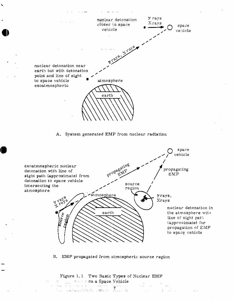
d any source region in contact with it and the electron transportaround it even in a vacuum.2 Consider some general space ve-hicle such as a satellite as shown in figure 1.1. Let us di-vide the EMP cases into two basic types: source region and nonsource region. Figure 1.1A shows the source region case wherethe nuclear weapon detonation point has a clear line of sightto the space vehicle so that an intense pulse of y rays and Xrays travels at the speed of light and produces high energyelectrons by interaction with the object thereby creating thesource region in the vicinity of the object. This is the sys-tem generated EMP. Of course there are EMP signals propagatedfrom the detonation point to the space vehicle but due to thesmall size of the source region these signals are not verylarge, at least from an EMP standpoint.3~4 In contrast to thissituation figure l.lB shows the case that a large EMP sourceregion in the atmosphere of the earth radiates an EMP out tothe space system. The detonation point may be deep in the at-mosphere or, of greater interest, it may be a high altitudedetonation with a quite large atmospheric source region with apropagation path missing the earth’s surface and reaching thespace vehicle after passing through a portion of the ionosphere.This propagated and dispersed EMP is not considered in thisnote, but there are techniques to simulate this which willhopefully be considered in some future notes.
Considering then the general case shown in figure 1.1A wehave the general problem of the system generated EMP plus othereffects associated with the nuclear radiation (of all types).For this case there are TRE phenomena in the system electronicsassociated with the same y rays and X rays (traveling at thespeed of light to the space vehicle) which also produce thesystem generated EMP. While our considerations here are pri-marily concerned with simulating the system generated EMP usinghigh energy photons, TRE interactions inevitably accompany suchsimulation.
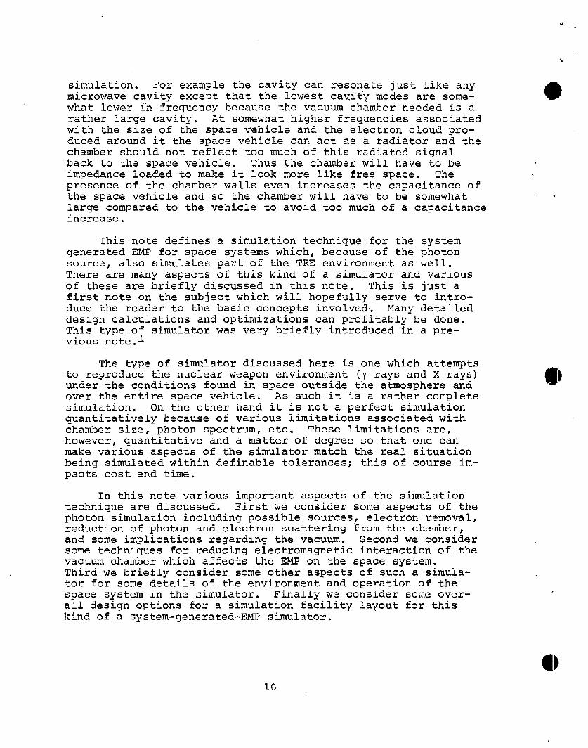
In the system generated EMP it is the presence of the sys-tem itself in the photon flux which produces the EMP source re-gion. As illustrated in figure 1.2 the y rays and X rays fromthe nuclear detonation travel from the nuclear detonation atthe speed of light and are essentially unattenuated on the wayto the space vehicle; the pulse width (time spread) is also es-sentially the same as at the detonation position. On interact-ing with the space vehicle these photons produce various ef-fects such as the direct TRE effects on the electronic
.
●6
t.
nucleardetonationclosertospacevehicle
‘“”””-/$’@
CJ,.fj$
~:nucleardetonationnear /
0earthbutwithdetonation 0
0pointand lineofsighttospacevehicle *’ atmosphereexoatmospheric
y raysX rays
*~ o space/0 vehicle
0
A. System generatedEMP from nuclearradiation
o space
,Hl vehicle
exoatmosphericnucleardetonationwithlineofsightpath(approximate)from
~$09%$.#~’’~~r::~ting
detonationtos~acevehicle .*/ ,.intersecting~h~ 0 ‘“ source /
A /atmosphere
----/- region /
yrays,Xrays
nucleardetonationintheatmospherewithlineofsightpath(approximate)fc]rpropagationofEMPtospacevehicle
.
B. EMP propagatedfrom atmosphericsourceregion
Figure1.1 Two BasicTypes ofNuclearEMP-‘on a SpaceVehicle

6’
#
thoseelectronspulledhack tothe space vehicleby theelectromagneticfieids
forward
electrons
InternalERIP isinsidethespace
vehicle
backwardejectedelectrons
ExternalEMPisindicated.1 indicatescurrent.A netpositivechargeisinducedon thevehicleinsideanegativeexternalspace chargeduringthefirstpartofthepuise.
Yrays and Xraysincidentfrom anucleardetonation
.
Figure 1.2 System GeneratedER4P on a Space Vehicle

components in the space system. Of concern in this note arethe high energy electrons emitted in various directions fromthe various parts of the space system and the associated elec-tric and magnetic fields and current and voltage densitieswhich produce currents and voltages at various places of con-cern in the system. This phenomenon is the system generatedEMP which can often be split into two types: external and in-
,- ternal. The internal EMP is associated with the high energyelectrons driven into the inner cavities of various kinds inthe system. For the internal EMP the electromagnetic geometryis determined principally by the space system itself, particu-larly if there is little penetration of electromagnetic signal!~to or from the system exterior so that the internal electromag-netic phenomena can be treated as occurring in one or moreclosed cavities. For the external system generated EM?, how-ever, the space around the system is also quite important.Thus for a simulation test with y rays and\or X rays incidenton the space system the proximity of other objects around thesystem which can influence the fields etc. can be quite impor-tant and has a significant impact on the simulator design.
There are other particles which travel from near the nu-clear detonation to the space system such as neutrons and highenergy electrons. However these particles arrive quite spreadout in time so that the pulse width, rise time, etc. are largecompared to transit times of interest on the space system andlarge compared to the y ray and X ray pulse widths. The spreaclin pulse width is also accompanied by a decrease in pulse am-plitude. The associated electromagnetic transients on thespace system are then also significantly reduced making theseparticle fluxes less significant from an EMP standpoint. Whileone could include various such particle fluxes in a simulatorof this type these are lower c)rderquestions, such as particu-larly in the case of neutrons which introduces other complica-tions such as radioactive activation of the simulator site andthe system under test.
In simulating the system generated EMP on a space vehiclethe space vacuum is quite impc~rtantso as to give the same non-linear electron transport in and around the space vehicle. Inthis note we consider a simulation approach for which the spacesystem is essentially at the earth’s surface. Thus some kindof vacuum test chamber to cont~ainthe space system is required.
L This chamber is the “space” pa,rtof the simulator, but it hasmany other features besides vacuum which significantly affectthe simulation. The chamber scatters photons and electronsproduced by a photon source such as a flash X-ray machine or anuclear weapon. The photon source is, of course, the otherfundamental part of the simulator and could be one or moreflash X-ray machines or even a nuclear weapon, say in an under-ground test context. Besides reducing the photon and electronscattering from the chamber walls there are various electromag-netic effects of the cavity which can interfere with the
.-—
simulation. For example the cavity can resonate just like anymicrowave cavity except that the lowest cavity modes are some-what lower in frequency because the vacuum chamber needed is arather large cavity. At somewhat higher frequencies associatedwith the size of the space vehicle aridthe electron cloud pro-duced around it the space vehicle can act as a radiator aridthechamber should not reflect too much of this radiated signalback to the space vehicle. Thus the chamber will have to beimpedance loaded to make it look more like free space. Thepresence of the chamber walls even increases the capacitance ofthe space vehicle and so the chamber will have to be somewhatlarge compared to the vehicle to avoid too much of a capacitanceincrease.
This note defines a simulation technique for the systemgenerated EMP for space systems which, because of the photonsource, also simulates part of the TRE environment as well.There are many aspects of this kind of a simulator and variousof these are briefly discussed in this note. This is just afirst note on the subject which will hopefully serve to intro-duce the reader to the basic concepts involved. Many detaileddesign calculations and optimizations can profitably be done.This type of simulator was very briefly introduced in a pre-vious note.l
The type of simulator discussed here is one which attemptsto reproduce the nuclear weapon environment (y rays and X rays)under the conditions found in space outside the atmosphere andover the entire space vehicle. As such it is a rather completesimulation. On the other hand it is not a perfect simulationquantitatively because of various limitations associated withchamber size, photon spectrum, etc. These limitations are,however, quantitative and a matter of degree so that one canmake various aspects of the simulator match the real situationbeing simulated within definable tolerances; this of course im-pacts cost and time.
In this note various important aspects of the simulationtechnique are discussed. First we consider some aspects of thephoton simulation including possible sources, electron removal,reduction of photon and electron scattering from the chamber,and some implications regarding the vacuum. Second we considersome techniques for reducing electromagnetic interaction of thevacuum chamber which affects the EMP on the space system.Third we briefly consider some other aspects of such a simula-tor for some details of the environment and operation of thespace system in the simulator. Finally we consider some over-all design options for a simulation facility layout for thiskind of a system-generated-EMP simulator.
.
10

L —.
—
II. Some Aspects of the Photon and Electron Environment
First let us look at the photon source which is going toinitiate electron motion on and thereby in the vi.ci.nityof thespace system. There are various designs of such sources thatone might consider. Some basic questions regarding the photonsource can be posed in terms of the incident photon environmentproduced over the test volume occupied by the space vehicle.Comparing various aspects of this environment (in terms of thephotons directly or in terms of the electrons knocked off aspace vehicle or other simplified object) to those associatedwith y rays and X rays from typical exoatmospheric nuclear det-onations one can estimate how complete certain features of thesimulation are i.neach_case considered.
For the photon environment there i.sthe general problem c)fmaking it intense enough over the entire space system. Supposethis environment is to be simulated as a photon flux passingthrough some cross section area As which might typically becircular with radius rs. This area can be thought of as thearea of a cross section area of a cylinder with the cylinderaxis parallel to the photon clirection from the bomb to thespace system. The space system is contained entirely withinthe cylinder. Of course the photons reaching the space systemcan be better thought of as in a cone, but this cone is verynearly a cylinder near the space system since the photons aretraveling very-nearly parallel at typical large distances fromthe bomb r (compared to rs) c)finterest.
If U is the entire energy released by the nuclear detona-tion* then the energy released as prompt y rays and as X rayswhich go far from the detonation position can be represented as
u= furYY
Ux z fxu (2.1)
The fractional energy in gamma rays fy may typically be a fewtenths of a percent which is somewhat less than say 3.5% whichis the fractional energy released as ganunarays in a typicalfission.5 On the other hand most of the energy comes out inthe form of X rays so that fx is close to one, say .7 or .8.The y ray spectrum is the fission spectrum plus that associatedwith neutron interactions with various materials and has an av-erage photon energy in the few MeV range. The average photonenergy of the X rays is much lower. Considered together the yrays and X rays give a photon spectrum which covers a broadrange of photon energies peaking toward the low energy end ofthis spectrum. Since the electrons emitted from the materials
*AII units are rationalized MKSA. While yields may bementioned in tons or energies in eV they must still be put intc}formulas in terms of joules.
11
(making up the space system) have energies which are a signifi-cant fraction of the photon energies, then the emitted electronspectrum is very dependent on the incident photon spectrum.The electron trajectories in the presence of the electromag-netic fields generated in and around the space vehicle are de-pendent on the electron energy. If the fields generated aresufficiently large the problem is then nonlinear making it de-sirable for a simulator to have as nearly the same photon spec-trum and photon pulse time history as a nuclear weapon, andsince photon spectrum can depend on the weapon design perhapsmore than one photon spectrum fordesirable.
For relating the y ray and Xons we have
1 ton S 109 calories
1 calorie = 4.1868J
so that.
1 ton s 4.1868 X 10⁹J
As an example then one might takecorresponding to an approximately
simulation testing would be
ray energies to typical weap-
(2.2)
,.
(2.3)
u= 10~6 J for the yield,2.4 megaton weapon. Suppose
,
as shown in figure 1.1 the nuclear detonation is exoatmosphericwith line of sight also exoatmospheric to a satellite in syn-chronous orbit so that the distance from the center of theearth is about 40 Mm. Let this distance also be the distancefrom the detonation point to the satellite. Also let fy = .002and fx = .8 to further specify the example.
In free space the photon energy per unit area falls off asUi(4~r2) where r is the distance from the detonation point.Thus the energy flux per unit area from y rays and from X rayscan be written as
‘Y f u@y=—=4~r2 y 4mr2
(2.4)Ux
+x=”—= fx~47ir2 4mr2
In these equations any asymmetry inincluded. Of course the y rays and
the weapon output is notX rays will not be uniformly
12

u
radiated into each increment of solid angle. If $r is the unitvector in the r direction th$n these results can include fac-tors which are functions of er which are normalized so that theintegral over the full solid angle (4r) is unity; the presentapproximation just has a uniform l\(47r)as this factor. Thesame applies to the formulas that follow in that er is not in-cluded in such functions as photon spectrum, etc. To i~cludeeffects of weapon asymmetry one may explicitly include er andintegrals over the solid angle, or one may use the present re-.$ults referred to any particular direction (i.e., particularer) with bomb yield, etc. ad:justedaccordingly.
The space system as seen from the weapon lies in an areaAs through which the simulator is to put photons. Taking As ascircular with As = nr~ we then have y-ray and X-ray energiesrequired as
(2.5)
Similarly one can define a tckal energy flux per unit area as
which gives a total energy referred to As written as
(2.6)
(2.7)
For our example case let r~ = 5 m and assume that this in-cludes solar panels and anything else associated with the spacesystem in the circular area As. Our example case for comparingsimulator performance (which will crop up throughout the note)can then be summarized as
Example weapon
[
U= 1016 J , f =Y
.002 , fx = .8
and (2.8)space system r = 40Mm , rs = 5 m
—
—
13

w
This implies
Example weaponand
space system
i
$0 ‘ .5 Jm-2 , 00=40J
$7 s 10-3 Jm-2 , @Y
=8 X10⁻²J (2.9)
0’ @.4 Jm-2 , .... =30J
Certainly from an energy viewpoint such numbers look quitetractable, even for a rather inefficient conversion of electronbeam energy to photon energy in a flash X-ray machine.
Not only might one consider the energy flux associatedwith the photons; there are various other characteristics ofthe photon flux which have significance to our simulation prob-lem. In its most general form the photons can be representedby a time dependent spectrum Sp with the normalization
(2.10)
The subscript p is used to denote photons (and similarly e forelectrons) and $ is used for particle energy (units are joulesin formulas). The units of Sp are then (Js)-~. The time vari-able implies evaluation of s
Eat some position in space, or for
our problem this could be ta en as retarded time
t* =ti-: (2.11)
since we are neglecting any atmospheric or other effects on thephotons propagating to the space system. While the limits onthe integrals are over -~ < t < m and O ~ *P < L=these can bereduced to only those values of t and Yp for which the spectrumfunction is non zero. Note that the spectrum function is writ-ten as a scalar; we are assuming that the photons are randomlypolarized with a uniform distribution in polarization angle. Apurely energy spectrum can also be defined as
/
!w
SPOJP) = -m p PS ($ ,t)dt (2.12)

which is then automatically asnormalized
/
m
S ($ )d$p = 1OPP
Having defined a
(2.13)
. spectrum function various parameters canbe defined suchsense as
as an average photon energy in a time dependent
(2.14)
per
the
‘avg
unitSince sp istime then
the number of ph,otons unit energy and
Jw
rip(t) s s ($ ,t)d+pOPP
(2.15)
is the distributiontime normalized as
function for
the
lumber of photons per unit
j
02
np(t)dt = 1-Cn
(2.16)
thenphoton pulseThe average photonbe defined as
for entire
!m
IJp (t)np-m avg
Tp =avg
=
(t) dt
.
H02 co
~ S ($ ,t)d~pdt-m OPPP
(2.17)

u
These spectral considerations can be applied to the y raysand X rays separately simply by using the subscripts y and x inplace of p. The distinction between y rays and X rays is basedon the physical processes of their generation in the nuclearweapon. From the viewpoint of the space system, however, bothare just photons and distinction can only be made on the basisof the energies +P of the individual photons. One might thenalso define a fractional energy of the bomb yield in photons as
fP
Efx+f=fxY
(2.18)
which is then approximately .8 for our example case. If onewishes an arbitrary split can be made in the photon spectrum ata $P of roughly 100 keV, calling those of lower energy X raysand those of higher energy y rays.6
The average y-ray energy Tyav is roughly 1 MeV and thedetailed spectrum is affected by tfleweapon design as evidencedby the fact that only a small fraction of the y rays escape.The temperature inside the nuclear detonation is of the orderof 10 keV corresponding to a 15 keV average particle ener y(3/2 times the temperature expressed in terms of energy).?Again the detailed spectrum of the X rays escaping from theweapon is affected by the weapon design as is discussed in var-ious classified reports as well as reference 6. While in thisnote we do not consider the detailed aspects of y-ray and X-rayspectra, the photon spectrum used in a simulator for the systemgenerated EMP will have a significant influence on the currentand charge generated on the space system.
As an example of an analytic spectrum function that isoften used consider the Planck or black body spectrum which wedesignate by Sb (time independent}. Let +0 be the temperatureof the effective black body radiator (which is 2/3 of the meanenergy in a simple case). With ~b as the photon energy, thenumber of photons in an incremental energy interval has thedistribution function7
(2.19)
Note that the distribution function for photon energy (insteadof number of photons) has a $3 factor instead of ~~. This dis-tribution is also often used in terms of incremental wavelength(instead Of in remental energy, or equivalently frequency) in
!5which case a $b term appears instead of +? for the energy dis-tribution.
.
16

.
From
Thusergy
Here we need the Riemann zeta function defined by8
2c(~) = k-a (Re(u) > 1)k=l
/
~a-l
= T+ ~“~dv (Re(a) > 1) (2.20)
the normalization condition of equation 2.13 we have
/[
m 2 i“b/$o1 =B ,+be 1-1d+b
o
= B@(3)L(3) = 2B@3) (2.:21)
our distribution function for photon number per unit en-is
For reference we have
C(3) = 1.202 ‘“”
G(4)m
= .900 ““”
(2.:!2)
(2.23)
The average photon energy fc~rthe black body distribution is
17

.
#
(2.24)
The peak of the black body spectrum (for photon number per unitenergy) is found from
Setting this to zero and calling the value of ~b for this peakas +bo we have
v~
[1+bo/*o
02-—=+:e ‘ - 2
(2.26)
which gives
as the spectrum peak. Note that this is less than the averagephoton energy.
Spectra like the black body distribution for X rays or thefission spectrum for y rays or actual measured or calculatedweapon spectra can be used for detailed transport calculationsto describe the photon interaction with the space system. Theresults can be compared with those produced by the photons froma flash X-ray machine. Of course an X-ray machine does notgive the exact same spectrum as a nuclear weapon. In particu-lar it is difficult and inefficient for an X-ray machine usingthe standard Bremsstrahlung production from an electron beam ona target to produce a photon spectrum with an”average photonenergy even approaching that from the weapon X rays. It istypically much higher, even in the MeV ranger but the hundreds
.
18

.
z
o. of keV range can and has been done with accompanying loss ofefficiency.
In order to compare various flash X-ray machines as photonsources for our simulator one can define several characteris-tics of the photon flux and see how they compare to the weaponflux. These characteristics or figures of merit should be
., _based on the various physical effects of significance which re-sult from the i“ncidentphot:on flux. We have already mentioned
‘-thetotal photon energy il~uminating the space system in the.- area As. However other large scale parameters can also be con-
sidered. These parameters can be thought of as weighted aver-ages of the photon spectrum with the weighting chosen accordingto the physics of particular important phenomena associatedwith the photon interaction. Thus one may reduce the considera-tion of the exact details of the photon spectrum and flux to afew numbers which characterize some of its most important fea-tures.
One of the macroscopic:parameters of the photons from theweapon is the dose rate which is the power deposited in thesystem of interest on a per unit mass basis. This has units ofwatts/kilogram abbreviated W/kg (preferred to rads/s or roen.t-gens/s). Integrating this over the entire radiation pulsegives the dose in J/kg (which is also the same as (m/s)2 or aspeed squared) . The dose and dose rate can be important forTRE interactions as an example. Another example would be thelocal energy deposited in a material simply from the viewpointof local heating and associated shock wave generation (at suf-ficiently large dose levels).
Now the dose and dose rate are not only functions of thephoton spectrum, but also of the atomic element or elementscomprising the material. I?urthermore the dose and dose ratecan vary as a function of position in the object (i.e. spacesystem) due to changes in the material composition and/or at-tenuation and scattering o:fthe photons. To estimate the dc)serate one can take a mean f:reepath for photon absorption intypical materials. Of course this varies somewhat between r~a-terials for any given photon energy, but if this is expressedin terms of a mass type of cross section (m2\kg) then the mate-rial density is factored out and the results only depend some-what insensitively on the atomic number (Z) of the material, atleast in the few MeV range where Compton scattering is dominant.Since for dose we are interested in the energy absorbed by t:hemedium then we do not want the total photon collisions per unitmass but instead the photon energy deposited. Thus we want themass absorption coefficient instead of the mass linear attenua-tion coefficient.
kg.this
Call this massFor any givenquantity as a
absorption coefficient M(~p) with units m2/atomic number Z one can calculate or look upfunction of +P the photon energy.9 This
19

quantity could be subscripted to indicate what Z or Z combina-tion this applies to. For low Z materials in the middle of theCompton region, say 1 MeV, M will be like .003 m2/kg. Forhigher photon energies pair production takes over (not very im-portant for our cases). For lower photon energies the photo-electric
frecess with an absorption coefficient proportional to
roughly Z /@ takes over.9 Thus at the very low photon energiesM is greatly increased and is very Z dependent.
One can define a mean mass absorption coefficient using agiven photon spectrum as
(2.28)
where the weight factor VP is used because we are weighting en-ergy absorption. Here we have used the time independent spec-trum although the time dependent form may be used as well togive
For a given Z or Z combination the mean mass absorption coef-ficient is then one useful macroscopic pararieterto character-ize the photons from the weapon or from another kind of X-raysource.
Call the dose rate waveform d(t) normalized such that
ICn
d(t)dt = 1-m
The total dose is then dporays) . This is related tonpo as
(2.30)
(and similarly for y rays and Xthe number of photons per unit area
Jm
d=P.
np M($p)~pSp(~p,t)d~p = fip 7P npo 0 avg avg o
/
(2.31)w
dp d(t) =‘P.
M(~o)~psp($p,t)d~p = Mp (t)@ (t)np rip(t)o 0 avg Pavg o
9
20

o wheretionsdosesation
subscripts, as before, allow one to separate the contribu-from various parts of a photon spectrum. Note theseare incident doses in that no attenuation or other alter-of the incident photon spectrum is included.
To get a feel for what the total dose is for our examplecase consider various photon energies and the associated mass
. . absorption coefficients for aluminum (using ref. 9) and the as-sociated doses for our 1016 J bomb at 40 Mm distance. For sim-plicity pick a monoenergetic photon spectrum and use that en-ergy for the calculations. Using just the total bomb energy ateach photon energy withenergy flux per unit areaing table.
opo ‘ .4-J-m-2 as the incident photonfor our example case gives the follow-
Photonenergy
10 keV
100keV
1 MeV
10 MeV
Table
Photonnumberfluxper unit
P)area (n
,*, x ,.’:{’
13 -23.1 X lo m
3*1 x # ~-’
,,~x # #
Approximatemass
absorptioncoefficient Approximatein aluqinum dose (d )
‘“I)A1) P.Al
2.4 m’/kg .96 J/kg
.0038m2/kg .0015J/kg
.0026m2/kg .001 J/kg
.0018m2/kg .0007J/kg
Approximateaveragedoserate(: )‘Al
.96X 108w/kg
1.5 x 10⁵w/kg
1 X 10⁵ W/kg
.7 X 105W/kg
2.1 Approximate Dependence of Photon Number Fluxper Unit Area and Dose on Photon Energy forMonoenergetic Photons from Example Weapon
As one can readily see the incident dose does not vary markedlyover the energy range 100 keV’to 10 MeV. However in going from100 keV down to 10 keV (and even lower) there is a very signif-icant change in the dose (associated with the photoelectricprocess) . Thus from a dose viewpoint (for a given incident en-ergy flux per unit area) the low end of the spectrum (belowabout 100 keV) can be quite important. The actual incidentdose for our example weapon depends on the detailed character-istics of the photon,,spectrmi and may be referred to other ma-terials besides alumlnum. This dose would seem, however, to beone useful comparison between a nuclear weapon (such as our ex-ample weapon) and a flash X-ray machine or other photon sourceas part of a simulator. Besides the total incident dose onemight similarly compare the incident dose rates based on thetime _history of the photon n~er and energy, comparing peaks,
0
rise times, etc. For our example weapon we might take a char-acteristic time of 10-8 seconds as a rough number for estimates.
21

.
Dividing the dose by this time (tp) gives an average dose rateduring.the pulse as
dP.
ap5—‘P
which is included in table 2.1.
(2.32)
As included in table 2.1 another useful number to charac-terize the photons is the number of photons per unit area.This is distinguished from the total energy per unit area ofthe photons. Let npo be the total (time integrated) number ofphotons per unit area at the space system, and szmilarly fornxo and nyo. Then nposp(~b) is the number of photons per unitarea per unit energy, nponp(t) is the number of photons perunit area per unit time, and nPosP(4P,t) is the number of pho-tons per unit area per unit energy per unit time. This numberof photons per unit area is related to the photon energy perunit area $po as
OP =1‘~pnp Sp(Vp)dVp = np ~po 0 0 0 avg
@po
‘P. = flPavg
Similarly in a time dependent sense we can write
Ja
OP OP(t) = $Pnp sp(vpft~dvp = +P (t)np rip(t)o 0 “o avg o
@p @p(t)
np rip(t)= ~ 0 (t)o Pavg
(2.33)
(2.34)
where @p(t) is the photon power Per unit area waveform normal-ized so that
22
(2.35)

4
This gives the time dependent photon number per unit area as
electron spectra associated with variousus choose a simple flat plate example of
4P (t)n“(t) = @
‘P. P P. Vp (t)avg
(2.36)
These formulas can all be applied to X rays and y rays by sub-stituting X and y respectively for p throughout. In additionto the energy per unit area a,nddose one can also look at thephoton number per unit area t:ocompare a nuclear weapon (as inour example case) to some other photon source for our simulator.Relating the energy flux per unit area to the dose gives
d ‘R+P. Pavg P.
(2.37)
dp d(t) = Mp (t)4P @p(t)o avg o
The mass absorption coefficient then provides a direct relationbetween the two kinds of quantities.
One reason to consider t;henumber of photons per unit areais because this quantity is related to the number of electronsemitted per unit area of the surfaces on the space system. Itis this emitted charge which is the source for the system gen-erated EMP. Each photon from the weapon or other source arriv-ing at the space system produces some number of electrons ~(!p) .These electrons have some distribution in energy +e and solidangle Q@ with respect to the incoming photons described by somedistribution function g($P,~61,Qe)normalized such that
,,
Hm
g($p,4e,Qe)dQed4 = 1\ o all Qe e (2.38)
Of course there can be some variation in rIand g depending onthe specific system geometry and materials and the position onany particular surface of the system from which the electronsare being emitted. There is also some time delay for the elec-trons to emerge from the materials but this is neglected in ourconsiderations.
Since there is much possible variation in the system geom-etry then some simple geometry would help in comparing the
photon spectra. Letuniform thickness,
23
uniform material composition,rection of propagation of the
and perpendicular to &r (the di-photons). Furthermore let the
flat plate be large enough that edge effects can be ignored andtreat the problem on a per-unit-area basis. Such a geometryquite naturally divides the electrons into two categories, theforward scattered and back scattered electrons which can be de-noted by subscripts f and b respectively on quantities such asthe fractional numbers of electrons aridthe distribution func-tions for energy and direction. There is still the question ofwhat plate thickness to choose for the standard of comparison.Since we are interested in the effects associated with largecurrent densities of these electrons then perhaps a thin plate,one electron range thick at the maximum electron energy associ-ated with a photon of energy ~p, would be appropriate.
Since the photon mean free path is generally much largerthan the range of an electron produced by that photon for mostenergies and materials of interest then we might consider anunattenuated photon flux in the material for this calculationof the electrons escaping from both sides. This avoids the is-sue of how thick to make the plate as long as it is thickenough to have reached the final equilibrium electron spectrum.Of course the photon mean free path is a strong function of $pat low photon energies (in the X-ray region) so that for agiven plate thickness which is thicker than the largest elec-tron range (associated with the largest energy photons) theplate can be many photon mean free paths thick at the low X-rayenergies giving a significant photon attenuation. Neglectingphoton attenuation in the plate then can lead to a significantoverestimate of the nuniberof low energy forward scatteredelectrons while having negligible effect on the backscatteredelectrons. Thus our present definition neglecting photon at-tenuation can be a useful way to compare electron yields fromdifferent photon spectra, but it does not give all the answers.For other comparisons one can just leave the plate thickness asa parameter in the problem.
Note that once the electron has left the system surface itis not followed any farther for the present comparison tech-nique. Further collisions of the electron with the system sur-faces can produce yet more electrons coming from the surfaces.In the case of large photon fluxes per unit area the currentdensity leaving the system can be large enough to make theproblem nonlinear, altering the electron trajectories. Itwould be desirable to make photon spectrum comparisons beforehaving to solve the nonlinear electron trajectories as a simplerway to understand something about the adequacy of the photonspectrum from a source of interest.
n
●
The dose comparison for the photon spectrum depends on thechoice of a material, particularly affecting the results forlow photon energies of interest. For the electron yield calcu-I.ationsone also needs to choose a material or regard this
24
choice as a parameter in the comparison. For first order corn-parisons one might choose a common material such as aluminum.Then an infinite homogeneous thick aluminum slab (for example)neglecting photon attenuation would form a basis for comparingphoton spectra (and numbers) on the basis of electron numberyield, energy, and direction, This type of comparison specifi-cation can be applied to the dose comparison as well.
Having defined a technique for comparing electron yields(such as, for example, the one discussed above) one can thenconsider various quantitative features of the electrons pro-duced. This characterizes some important features of the elect-rons in a few numbers. The fractional number of electrons (c)relectron yield) produced by the incident photon spectrum isfound by ~ver-ag”lngover fi($p)for both time and energy as
This
. .
can be considered an electron ~enerationrelated time dependent elect:ronefficiency
so
Jco
6= (t)np(t)dtPavg -w ‘Pavg
Typical electron fractions
(2.39)
efficiency. Acan be defined as
(2.40)
r. r.= JJ n(~p)sp(+p,t)d+pdt (2.41)
-m o
are somewhat dependent on the inci-dent photon spectrum as well as the material of interest.Again aluminum is used as the material for making comparisons,In reference 6 an estimate is made of the electron fraction as-sociated with incident X rays, giving an electron fraction ofabout 5 x 10⁻⁴ at a $
$of 30 keV with a dependence of about l~fil
far from absorption e ges. Another reference summarizes someof the spectra and electron fractions for incident X rays show-ing the increasing electron fractions for low photon energies,,loFor $
Eabout 5 keV the electron fraction can be a few percent,
The p otoelectric process which dominates the low energy photoninteraction has a large influence on this kind of electron frac-tion variation. Going to higher energies for yMeV rangeprocess.about 7 x
the dominant photon interaction is byThe electron fraction for10-3 (as in reference 6).
25
such photoiVarious of
rays in the fewthe Comptonenergies isthe theoretical
notes deal with electron fluxes in air associated with MeV pho-tons. Calculations have been made for various photon spectragiving, for example, an electron fraction for forward scatter-ing of 3 x 10⁻³ for a fission y-ray spectrum.1~
The electron fraction discussed here has been for electronsemitted from both sides of the assumed infinite slab of alumi-num. one can use ~f($p) for a forward scattered fraction andvb(~p) for a backscattered electron fraction. For low photonenergies for which the photoelectric process is dominant theelectrons are made to move initially at about a right angle tothe incident photons. This results in roughly equal magnitudesfor Vf and rib,each roughly half of ~. As the photon energy is’increased the Compton process takes over and the electrons areejected predominantly in the forward direction. This resultsin ~f approaching rlwhile qb becomes a small fraction of U.
Having the electron fraction in various forms we can lookat the total number of electrons and associated current density.The number of electrons per square meter leaving the slab fromboth sides can be written in time dependent form as
/
02
ne ne(t) = nP
v($p)sp(~p~t)d+p =o 00
where the electron emission waveform
~
mne(t)dt = 1
-m
The total electron emission per unit
(t)np rip(t)‘P
(2.42)avg o
is normalized so that
(2.43)
area is then
/
m
n =e ‘Po’ -mnPavg /
(t)np(t)dt = n ‘v (Tp)Sp($p)dOpo P00
= : (2.44)Pavg‘P.
The current density, taking all leaving electrons from bothsides as contributing with the same sign to this current den-sity (even though oppositely directed) is just
26

*
o Je(t) = -e ne ne(t)o
(2.4!5)
e = 1.602 ’00 X 10-19 C
where e is the magnitude of the electron charge and Je is thenet current density leaving. The total charge per unit areaemitted is
Jco
sie‘“ Je(t)dt = -e ne-m o
(2.46)
If one wishes, the electrons per unit area, current density,and charge per unit area can be separated in forward and back-ward components with subscripts f and b respectively simply byusing ~f(~p) and ~b($p) in the inte9rals.
The number of electrons per unit area can also beto the incident photon energy per unit area (which canveniently measured) from equation 2.33 as
‘avg ~n =e.
Vp ‘oavg
which requires that one knowerage electron fraction. In
the average photon energy
relatedbe con-
(2.4’7)
and av-
ne ne(t) =‘avgYP
(t) @p Op(t)o“ oavg
a time dependent form this is
(2.4:3)
The current density and the associated charge emitted from thesurfaces of a space system are clearly important effects of theincident photons from an EMP point of view. This places greatimportance on the average electron fraction. If the photonsare specified in terms of energy flux per unit area then theaverage photon energy is also very important. Sometimes theincident photons may be specified in terms of dose. Then fromequations 2.37 we can write
27

.
.
fip davg P*
n =eo VP =P
avg avg
ne ne (t) =o
(2.49)
‘Pav(t)dp (t)
o$P (t}Mp (t)avg avg
. .
In such a case it is also important to know the mass absorptioncoefficient.
While the time dependent current density of electronsemitted from the space system is one of the most important pa-rameters to consider in designing a simulator for the systemgenerated EMP on a space vehicle, other parameters also affectthe resulting EMP. The resulting current and charge densitiesin the space inside and outside of the space system depend notonly on the emitted charge but also on the subsequent spatialand temporal behavior of the electrons. This subsequent behav-ior depends on the energy and direction of the emitted elec-trons as well as the number of electrons. Remember that forlarge numbers of electrons the problem is nonlinear. Thus onemust be concerned (for the larger current levels in particular)with the average energy of the emitted electrons and how thiscompares to the energies associated with the position changesof the electrons in ‘the electromagnetic fields. The vector andscalar potentials may be more convenient for considerations ofthe electron energy +e. For example in the static limit onlythose electrons with $e/e greater than or equal to the negativeof the scalar potential of the space system with respect to in-finity can possibly escape from the space system. While theaverage electron energy does not completely characterize theinteraction of the electrons with the fields it still is a firstorder way to compare different electron spectra for the fieldsthey will produce.
Again for our infinite aluminum plate one can separate theelectrons into forward and backscattered parts and consider anaverage energy for each with appropriate subscripts added tothe following results. With the electron fraction rl(~p)anddistribution function g($Pr~e,Qe) (normalized as in equation2.38) we have the time dependent spectrum of the electronsemitted at each time as
28
.
with
In a
with
e
/
_l”wn(VP)9(I$
fip oavg
the normalization
time independent
se (ve,Qe,t)d~ed$edtP
sense this is
Ilx
se Weme) = se (veirQe,t)dtP -m P
the normalization
Hw
se ($e , Qe)df~ed$o all Qe p
e
Adding subscripts f and b with thedians or half a sphere
1
(2.51.)
(2.52)
(2.53)
normalizations over 27Tstera-
29

.
forward
backward
and usin’gthe presumably known ~f and rtbwhere
Tlf+?lb=rl
(2.54)
(2.55)
then sepf($e~~e,t), Q t), Sepf($e,fle),and Sep ($e,~e)Rote that‘ep~(~~’t~~ same manner as above.are all readily obtaine
this also invo~ves Calculating ~pfavg(t) and ~pbavg(t) as wellas ~Pfavg and ~pbavg.
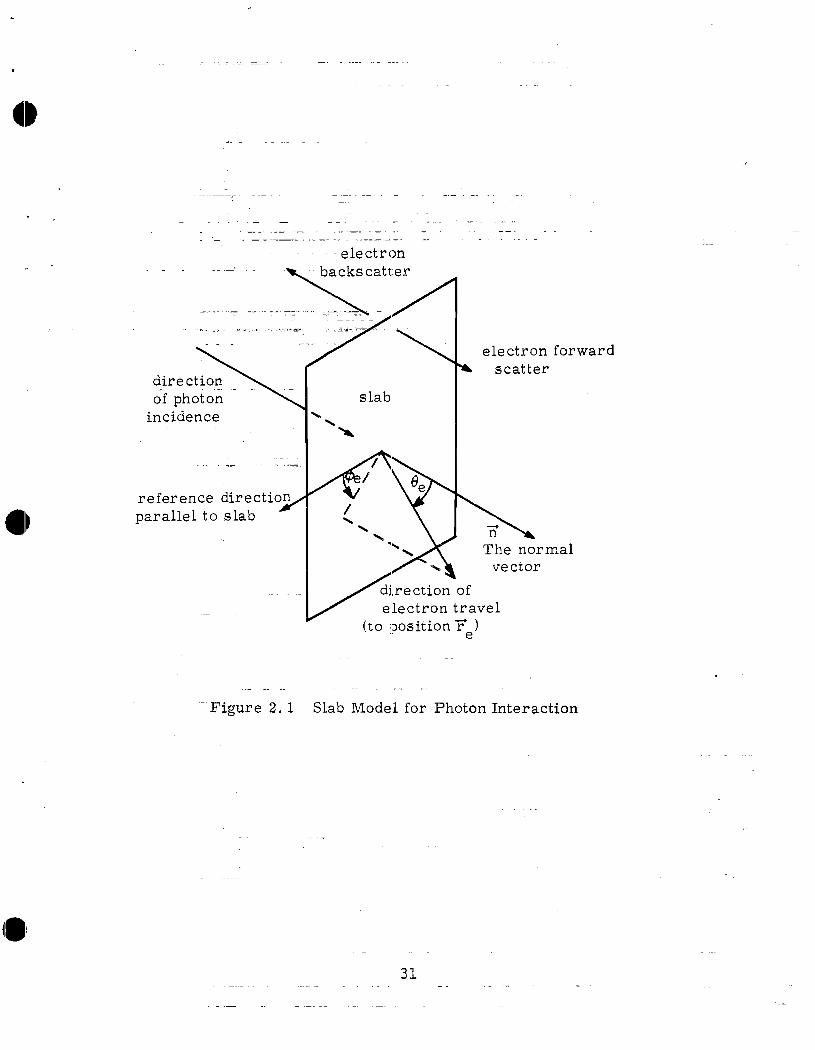
Figure 2.1 shows an infinite slab which is perpendicularto the direction of incidence of randomly polarized photons(with uniformly distributed polarization angle). Consideringthe electrons emitted from some incremental area of the slabthen by symmetry their directional distribution is uniform withrespect to @e and onl
$depends on ee where Oe is the angle from
a normal to the slab and @e is the azimuthal angle around thisnormal from some arbitrary reference axis parallel to the slab.Forward scatter has O ~ 6e < ‘Ir/2and backscatter has m/2 < ee< x. The electron distribution function for this slab geometry~an be written as
(2.56)
I
where g is still considered on a per-unit-solid-angle basis.The normalization is now
H‘m 2’IT
J
‘lTgs(Vp,$e,6e) sin(ee)d$ed~e = 2W gs($p,+e,ee) sin(0e)d6e
00 0
= 1 (2.57)
since the incremental solid angle is just
d~e = sin(ee)d$edfle
30
(2.58)
.
,
0
.,
.-
.
electron
‘-\directionofphotonincidence
referencedirection/
parallelto slab
slab
electronscatter
forward
\ xThe normal
d )l! g
e
/\\\
‘\\
-%
/
vector
directionofelectrontravel
(topositionT’e)
Figure 2,1 SlabModel forPhotonInteraction
.
Subscripts f and b can be used with gs as well as with g.
Besides the electron ‘energy being considered one mightconsider something about the electron direction as well. Onemight look at the average velocity to see how fast the charge ismoving away from the slab. For O < f3e< m/2 the average veloc-ity of the forward scattered electrons is reduced in magnitudebeca~se they are not all traveling parallel to the normal vec-tor n (or along ee = O). The velocity of an individual electronis given by
i
*
.-.-
. .
22
“[()]
1/2
+ mecVe($e?eef$:) = 1 - ~ c:re
(2.59)
where
2’mec = .511 MeV
z 2.998 x 10⁸ m/s
c=&’
(2.60)
and where ~ is the electron rest mass, c is the speed of lightin vacuum, P. is the permeability of free space, So is the per-mittivity of free space, and ere is a unit vector in the direc-tion of electron travel. For the slab model we have the averageelectron velocity for the forward scattered electrons at thetime of electron emission as
forward
32

.-.
0 and similarly for the backscattered electrons by changing sub-scripts f to b and changing the limits on the 13eintegration to‘lT/2< @e < ~. By integrating C)ver-m < t < @ after multiplyingby n~f(t)–(or neb(t)) time ind~~pendentaverages are alSO ob-tained. Remember that nef(t) and neb(t) are normalized so thatthe complete time integral is cme.
The average electron energy is a significant fraction ofthe energy of the photons producing the electrons. For low en-ergy photons for which photoelectric interaction is important
- the initial electron energy is most of the photon energy but itloses energy on moving through the slab. Those that leave theslab can then have roughly half of the photon energy on the av-erage. At higher photon energies for-which the C6mpton processis dominant the electron is initially produced at a significantfraction of the photon energy, say half, making the escapingelectrons still have say a quarter of the incident photon en-ergy. Thus average electron energy is closely related to aver-age photon”energy and in the example problem using monoener-getic photons in table 2.1 the electron energy would have aboutthe same variation as the photc)nenergy. In considering a dis-tributed photon spectrum, however, the variation of the elec-tron fraction rl($p)has some influence, weighting the electronenergy toward those +p values having the larger rI. The averageelectron velocity is strongly influenced by the electron energyand therefore by the photon energy in line with the above dis-cussion. However, the velocity is not simply proportional tothe energy, shifting the averaging somewhat. The electron an-gular distribution as a function of 6e also varies with Yp and+e, also shifting the averaginq process somewhat. Still theseare generally small factors compared to the dominant influenceof the photon energy and even electron fraction dependence onphoton energy.
In this section various aspects of the incident photonspectrum and number per unit area have been considered from theviewpoint of average quantities associated with resulting ef-fects of the photon interaction. This reduces the photons tosome discrete numbers such as energy flux per unit area, numberper unit area, average photon energy, average mass absorptioncoefficient, dose, average electron fraction, number Of eleC-trons per unit area, average electron energy, average electronvelocity, and photon pulse characteristic time. Note that manyof these quantities require the definition of an idealizedspace system such as an aluminum slab one electron range thickand perhaps neglecting photon attenuation in the slab. Manymore characteristic numbers can be defined if one wishes. Ingeneral it will be a difficult task to exactly reproduce thedesired nuclear weapon photon spectrum in a simulator using saya flash X-ray machine. However one must have some way of judg-ing if he is even getting close or which parameters are beingexceeded and which are deficient. This allows for progressive
33

.
improvement in theare rather naturalism (as elaborated
simulation. The parameters discussed hereones and these with their associated formal-above) should form a useful basis for char-
acterizing photon sources for both calculational (design) pur-poses and experimental measurements.
.-.
.-
034
. .
.
@III. Some Aspects of the Photon and Electron Simulation
A photon source for the simulator must illuminate a spacesystem with a photon flux over some area As (= nr~) which wetake as circular (for convenience) with radius rs. One part ofthe simulator design is this photon source. The total simula-tor involves much more than just the photon source, such as thevacuum tank to hold the space system and various equipment as-sociated with the vacuum system. Thus one might even have morethan one X-ray machine, for example, for different photonsources. One might also start out with a not very large flashX-ray machine and as time goes on replace this machine withprogressively better machines.
There ar~ ‘va”rioustypes of pulsed photon sources one mightuse for such a simulator. In order to closely approximate thedesired weapon photon spectrum and time history one might use asmall nuclear device in an underground test context. Due tothe required vacuum system for the space system environment anunderground test could be rather difficult. The lack of re-peatability on any short time scale limits the usefulness ofsuch tests. Nevertheless duplicating the weapon X-ray spectrumcan be very difficult for a large flash X-ray machine becauseof the comparatively low photo:nenergy for which such X-ray ma-chines are quite inefficient given the present state of the art,Thus one cannot completely dismiss the possibility of nuclearweapon sources for the simulator. While most of the discussionof the simulator design assumes the use of flash X-ray machinesources the same design features for the remainder of the simu-lator can be applied for the most part in the case of a nuclearweapon source or other type of pulsed photon source.
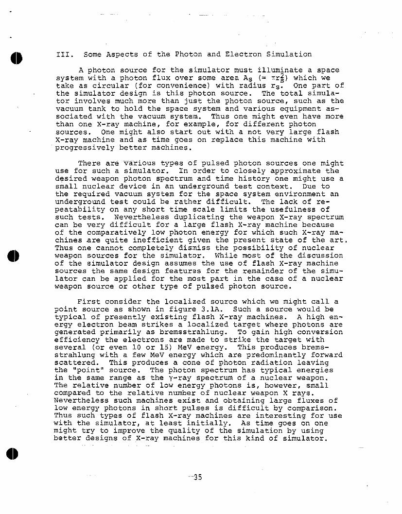
First consider the localized source which we might call apoint source as shown in figure 3.1A. Such a source would betypical of presently existing flash X-ray machines. A high en-ergy electron beam strikes a localized target where photons aregenerated primarily as bremsstrahlung. To gain high conversionefficiency the electrons are made to strike the target withseveral (or even 10 or 15) MeV energy. This produces brems-strahlung with a few MeV energy which are predominantly forwardscattered. This produces a cone of photon radiation leavingthe “point” source. The photon spectrum has typical energiesin the same range as the y-ray spectrum of a nuclear weapon.The relative number of low energy photons is, howeverl smallcompared to the relative number of nuclear weapon X rays.Nevertheless such machines exist and obtaining large fluxes oflow energy photons in short pulses is difficult by comparison.Thus such types of flash X-ray machines are interesting for usewith the simulator, at least initially. As time goes on onemight try to improve the quality of the simulation by usingbetter designs of X-ray machines for this kind of simulator.
.—
35
* gridshieldto suppressJ noisefrom pulserand
.
associatedelectronscatcher ~
forelectron:i ocollimator
k beam , 1 #“-vac&um_ ~ .-. - 1photonsource
!3{ ;
. #-”-1
II
I(electronbeam
+
---- r I 10
target) /-:- S1 Ic outer-— .....kr z o~
volume~: I boundarycentralaxis———— ——9 e~-————— ——— —— --f
Containhlg _
ofphotonbeam I ofphoton”t photon?.
l%
_E<hotons I s;%: [ beamI and --- t I
I electrons-\_
electron :I
-wrerriovalI
--- -:<___ :I region : ---1 L’-
-use magneticandf~ II I1 or electricfields : I
A. Pointsource
electronremoval gridshieldto suppressregion. ~oisefrom puker-and
collimation
Y~~associatedelectrons
region .r’ --r
M1:
t I I [.photon& I I I~source I 111.region i 111:
t I I 1:I I I 1:I [ I l:—I i 1 l:’I I I 1:[ II 1;I I I 1.I Ill:I Ill:LT Ll_J: .
I .
vacuurfi ~--- 7I 11, If volume I, containing
centralaxisofarray space i——— ——— ——— —ofphotonbeams I system I
1 I
I I
f (t I-----1
B. Distributedsource
Figure 3,1 Two Kinds ofX-Ray Sources
36

● ✎✍✎
.
0 Typical high photon eneugy point sources for this kind ofsimulator can be characterized by some half cone angle 9C as infigure 3.1A. This angle is chosen so that for O < 0 < 6C thephoton flux has some desired degree of uniformity: C~llimatethe photon cone at this angle to get rid of unwanted photonsthat can interact with the simulator structure but are not go-”ing to be used to interact with the space system. If ~ is thedistance to the space system from the approximate point sourcethen the photon simulation radius rs is just
r = 2 tan(flc)= !Lec[l+ 0(0:)]s for Oc + O (3.1.)
Then given rs because of the size of the”space system thispoint source can be positioned so as to just illuminate all thespace system. Given the total photon number, energy, etc. inthis cone then the maximum densities (on a per unit area basi%)available from this source a:refixed basically by dividing byAs.
For comparison to our example 1016 J weapon at 40 Mm dis-tance as in equations 2.8 and 2.9 and table 2.1 we have pickedrs =5m. Let us also briefly look at typical large flash X-ray machines. For sake of discussion consider the operatingcharacteristics of the Hermes IX machine.~2 This produces a ’70ns wide bremsstrahlung pulse from an electron beam with elec-tron energies of roughly 10 MeV giving a 4000 rad dose (in wa-ter) at 1 m from the tantalum target. At 9° off the beam axisthe photon dose is down to about .6 of the axial value. Thusfor our example machine (neglecting dose conversion from waterand noting that 1 rad is 100 erg/ginor 10-2 J/kg) we then take
exam-piemachine
Given the rs
examplemachine
andspacesystem
[“ec ~ .05 IT= .157 radians
(3.2)dP.
= 40 2-2 J’/kg
value we have
[
rs =5m
2= 31.5 m
d=P.
.04 J/kq
(3.3)
37

.
.
Comparing this dose to what appears in table 2.1 we see thatthis is more dose than our example weapon would give if all ophotons were 100 keV but less dose than it would give if allphotons were 10 keV. Thus a Hermes II type machine looks inthe ballpark as far as dose is concerned, but this neglects ‘many subtleties. The weapon has a distributed photon spectrumfor which the dose (or perhaps the dose that penetrates to acertain depth.of aluminum) must be evaluated. .,
There are, of course, various other comparisons betweenthe example machine (with space system) and the example weapon(with chosen distance). For example the photon pulse from Her-mes II has a pulse width of 70 ns while for our example weaponwe use a nominal 10 ns for a characteristic time. The averagephoton energy for our example machine is a few MeV while theweapon photon spectrum is dominated by the X rays with muchlower energy. The same discrepancy is then also noted for theaverage energy of the electrons emitted from the space system(using the previously discussed slab model) due to the closerelation of the energy of the emitted electrons to the energyof the incident photons. Considering the average electron ve-locity a 1 MeV (not including rest mass) electron has a speedof about .94 c while a 10 keV electron has a speed of about .2c. Of course there is some difference in the direction of theemitted electrons but the relative speeds are somewhat closerthan the relative energies.
Convert the dose to energy per unit area through a massabsorption coefficient. Taking an average photon energy13~Z4of 1.6 MeV we have a mass absorption coefficient of about .0025m2/kg. Then the energy per unit area and number of photons perunit area are
examplemachine
andspacesystem
Comparing the
“Op = 16 J/m2o
= 1 x 10¹⁴ m-2.nPo
(3.4)
number of photons per unit area to the resultsfor the example weapon in table 2.1 the comparison is not un-favorable except for very low average weapon photon energies.One would come to a similar conclusion about the comparativenumber of electrons per unit area emitted from the idealizedspace system (slab model) . The energy per unit area is muchlarger than that for the example weapon (equations 2.9). Thusour example machine for some parameters exceeds the exampleweapon while for other parameters the example machine is defic-ient. Thus existing flash X-ray technology can do a partialsimulation of the weapoh photons to the required levels. How-ever, some aspects are not closely simulated indicating that
38
.
.
0further development of such X-ray machine technology is neededto better tailor the photon spectrum. The above results indi-cate that some parameters can even be reduced if needed (suchas the photon energy flux) in the process of better tailoringthe photon spectrum. In building a simulator for the systemgenerated EMP on space systems one might even begin testingwith a particular X-ray source and then change it for somethinf3better as tests become more detailed and sophisticated and bet-ter X-ray source technology is available.
One of the directions one might pursue in developing bet-ter fiash .X_-ray__m_achige.SEOz..thi.sapp+igqki.on +s,the distribu-ted photon source concept as illustrated in figure 3.lB. Thiskind ‘of simulator does not require large photon fluxes oversmall areas. The space system is generally quite large com-pared to the usual exposure volumes used in TRE tests withflash X-ray machines. Why start with a very intense photonflux over some small area and then expand it to a large testarea? By spreading out the photon source over dimensions com-parable to the space system size the photon intensity near thedistributed source need be no larger on the average than thephoton intensity at the space system. One might even tailorthe direction and intensity of the photons coming out of thesource to improve the uniformity in spectrum, numbers, and di-rection at the space system. Having a much larger photonsource area one can generate more photons, generate a betterphoton spectrum, and/or have a better time history of the pho-ton pulse. There is now more space in which to cram electronbeams, anodes, etc. allowing o“neto improve various aspects ofthe photon output.
This kind of photon source might typically be an array ofsmall sources_ (cathodes, electron beams, and anodes) arrangedin a pattern of unit cells which fit toge-theras simple planargeometric figures such as squares, regular hexagons, and equi-lateral triangles. Each cell can have its own return currentpaths, returning the beam current, thereby isolating an elec-tron beam in one cell from those in other cells. Thus an arrayof photon sources can reduce the problem of generating highcurrent electron beams and make it easier to lower the electronenergy in the beams and thereby lower the average energy of thebremsstrahlung, although at a decrease in conversion efficiency.One might integrate all these individual sources into a morecontinuous source provided return currents are distributedthroughout the electron beam which is traveling toward thebremsstrahlung target. Such current paths, say on small wires,,can effectively isolate one part of the beam from another.Such added current paths can be oriented such that some areparallel to the electron beams while others are perpendicularto the beams to effectively alter some of the macroscopic fea-tures of the ratio of electric and magnetic fields associatedwith the beams (or beam array) . The added current paths mightthen be oriented at some optimally chosen angle to achieve
39

.
similar effects. If standing waves of the electron beam insuch a structure are troublesome one might introduce some ran-dom variations in the positions of such current paths dependingon the details of ,the problem. Figure 3.2 shows some variousneutralizing current path geometries one might consider. Ofcourse for some cases one may not drift the beam but positionthe cathodes fairly close to the anodes so that while the mag-netic field neutralization is needed the electric field neu-tralization is avoided. However if the cathodes, or some ofthem, are far b&hind the anodes to reduce packing problems and/or to spread out the cathodes over a larger area than the anodearray (thereby having a convergent electron beam array) thenbeam drifting is required and gases, metallic conductor arrays,and/or some combination of the two might be profitably used.In addition a magnetic field parallel to the beam may help incontrolling it. In a beam array such a guide field may need tobe periodically reversed to keep the guide magnetic field linesclosed on themselves so as not to significantly fringe out tothe space system.
The cathodes and anodes can also be designed to fit intothe distributed photon source array. The cathodes can be sepa-rated from one another or some other technique can be used toallow the return current paths to pass through the cathode re-gion so as to isolate portions of the electron beam array fromone another. Each cathode might be further segmented in vari-ous designs such as are used to obtain good field emissioncharacteristics as required for the beam admittance (or perhapshere admittance per unit area).
Perhaps more significantly the anode can be split up inseveral ways to improve the conversion efficiency from elec-trons to photons, particularly low energy photons. This can beachieved by using multiple anodes for the electron beam to passthrough consecutively, each anode being only an appropriatefraction of an electron range thick. The direction to the tar-get would be off at some angle from the beam so that the lowenergy photons which are produced somewhat isotropically onlyhave to travel part way through one of the anode foils on theway to.the space system. This is compared to each electron inthe beam which passes through a large number of anode foils.Another way to achieve this effect is to make the electron beammake multiple passes through a single thin foil. If the passesare all through the same area then the local space charge den-sity is increased, limiting the current density somewhat. Themultiple pass might be achieved through electric fields by puls-ing the anodes positive with respect to the cathodes which areelectrically grounded to the pulser body. One might have twocathodes to each anode, one on either side producing two elec-tron beams traveling in opposite directions. If one of thecathodes is in the way of the desired photons it could be madeessentially transparent by making it look like a screen wheremost of the cross section area would be holes. To this dual
.
40

.
, 0 indicatesthepositionofan electronbeam.
@) and @ indicatepatternsofalternatedirectionsforguidemagneticfieldsin
9B adjacentcellsforcasesoftriangular
● indicatesthepositionofand squarecells.These requireadditional
a currentreturnconductor.coilsor permanentmagnets. Forhexagonalcellsalternatingdirectionscan se accomplishedingroupsofcells.
● ● ●
triangularce11s
A. Some geometries
square“cells hexagonalcells
forreturncurrentpaths
pathsparalleltobeam
togetherwithbeams inarrays
I
Some pathsalsopointoutofthe
page,
Some pathsalsopointoutofthe
page.
pathsperpendicularcombinedtobeam paralleland
perpendicularpaths
Egcd
Most pathsparallelto
are notthepage,
B. Currentand chargeneutralizationconductingpaths
9)distributedinelectronbeams
pathsatangletobeam
Figure3,2 DiscreteCurrentand Charge NeutralizationConductorsinE;lectronBeams and Beam Arrays
41

.
cathode arrangement one could also add a guide magnetic fieldas well as various additional beam directing conductors andgases. Figure 3.3 shows some of these numerous possibilities.
Magnetic fields can also be used to make multiple passanodes. One can simply make the electrons race around as in acyclotron by using a magnetic field perpendicular to the elec-tron beam. The electrons could be made to strike the same foilonce or twice in one circular path. One or more special en-trances for the electron beam(s) would be needed to inject theelectron beam(s) into the transverse magnetic field. In such ascheme multiple foils could also be used and the approximateelectron paths need not be circular (or spiral as a better ap-proximation) but might be helical (with a spiral decay). An-other scheme might have oppositely directed magnetic fields onopposite sides of a foil, both fields being parallel to thefoilt by having the foil itself at least transiently carry partof the guide-field-producing current. Such a combination ofguide magnetic fields would make the electrons circle in oppo-site directions on opposite sides of the foil and thereby makethe electron cloud drift along the foil as the electrons passedback and forth through it. Clearly there are many schemes formaking electrons make multiple passes through thin foils so asto reduce the attenuation of those low energy photons producedin the anodes which are headed toward the target. Perhaps somecombination of electric and magnetic field geometries with foilgeometries such as those above will prove optimum.
As part of an optimum anode design one can control therelative distances that electrons and photons of interest travelthrough anode foils. Since the space system is in one generaldirection from the anodes then the anode foils can be alignedsuch that their surfaces are approximately perpendicular tothis direction. The photons of interest then have a minimumfoil thickness to traverse. However the electrons in the beamsneed not travel in this same direction. Their paths througheach anode can be significantly larger than the foil thicknessby striking the anode at some optimum grazing incidence angle.Thereby the electrons can deposit a greater fraction of theirenergy while still keeping the foil thin to allow more of thelow energy photons to escape in the direction of interest. Theratio of electron travel distance through the foil to the foilthickness is then greater than one and can be thought of as oneof several possible figures of merit for the anode array design.
Since the lowest energy photons that propagate to the spacesystem come from the last part of the foil thickness (becauseof the high photon attenuation in the foil at sufficientlysmall photon energy) then the foil might even be laminated orcomposed of several thinner foils. The foil nearest the spacesystem would be chosen to have atomic number Z to optimize toproduction of the very lowest energy photons. The next foilback would be designed with slightly higher energy photon ●
42

.
0
direction to
/
I direction to
t
I direction
system underI
systemI
to systbm
test
I I
1 I1
I
secondelectron I
second
:::? I ~,< ! *
elect ron
electron
, ,-electron
Ielectron I electron
beam beam
. . I
multiple anodes perpendicular I multiple anodes slanted
to beam1“
at same angle to beam
pxsibleguide
magneticfield
!
A. Multiplethinanodes
direction
ft
I
to system cathodes in thisdirection should I
be mostlytransparent. I
1
electronbeam
1
I
-4
I
anode typical
+I
electron
t
pathI
electronbeam I
I
anode pakeci positive withrespect to one or more I“grounded” cathodes. ..-
I
directionto system
1
‘ @ %%::cthe electrons
.*
electronspiral
anode
rin~t electronIx?am (shieldedfrom magneticspiraling field)
b
electron beam spiraledin magnetic field
1 beam
I
I multiple anodes slantedin alternate directions
II
I directionto system
t
@ magnetic
I
field
I I
electron
~anodeeu-4re.tI
It
for field
input @ magnetic
I
electronbeam
fie Id
1‘ (shielded)
! reversed magnetic fieldon opposite sides of anode
Et Multiplepass ofelectronbeam throughone anode
direction to
4
electrons have some spreadsystem in direction of travel due to
I scattering.
‘~ 4
morephotons
path of typical I
incidentphoton in anode
L to additiona 1r
electron beamfoils
for electrons
electrons withreduced energy
C. Increasingratioofelectrontophotontraveldistanceinanode
Figure 3.3 Anode Geometries forTo Photon Conversion
IncreasingEfficiency
Electron
43
production in mind, and so on with successive layers. It isnot clear how much improvement if any one can achieve this waybut it is something to consider.
Now we don’t want photons going everywhere with all direc-tions in this simulator. We wish to illuminate only the spacesystem, and illuminate it with photons traveling in approxi-mately one direction. A technique which should then be consid-ered is collimation. First consider collimation in the case ofa single point source as illustrated in figure 3.1A. The con-cept of collimation is rather straightforward in this case. Atsome position between the idealized point source and the spacesystem place a thick photon attenuator with a hole in it whichallows only those photons directed toward the space system topass through the hole, the rest being severely attenuated.There is some scattering of photons off the “edge” of the col-limator hole but such scattering can be considered in the de-tailed design of the collimator. Multiple collimator assem-blies can be considered so as to improve the overall co2lima-tion. Generally one would like the collimator assembly to befairly close to the photon source so that the collimator assem-bly does not approach the space system so closely so as to makethe other items which come after the collimator be placed un-necessarily close to the space system and thereby increase someof the electromagnetic distortion associated with the presenceof the simulator structure.
lf one uses the distributed source type of photon genera-tor as shown in figure 3.lB then the collimation problem issomewhat more complex. If one attempts to collimate the photonbeam as a whole then the distributed photon source must bemoved far away if it is to look like a point source for a col-limator to effectively remove the photons not directed at thespace system while removing no photons which are directed atthe space system. Such a collimator for the whole beam thendoes not look very attractive because a far away photon sourcemeans small efficiency in getting photons to the space system.If one notes that the distributed photon source can be made ofmany small sources, such as indicated by the patterns shown infigure 3.2, then the collimation can be done fairly close tothe distributed source. Each small photon source can be colli-mated in a manner like that shown in figure 3.1A for a singlesource. Each small source would then send a photon beam througha collimator at its own optimally chosen angle to illuminatethe space system (and very little more than this).
One of the undesirable byproducts of the photon source iselectrons directed toward the space system. These need to bedeflected away from the space system such that they do not en-ter the test chamber. Note that one cannot simply stop thesewith a slab of material because the photons knock electrons offsuch a slab to replace the removed electrons. Perhaps the
44

.
,
ecurrent of such electrons can be reduced, at least for the low
energy electrons by having a very thin layer of low Z (atomicnumber) material as the last material on the photon source.This layer would be one electron range thick at some appropri-ate small electron energy. This layer should be thin enough tc)not appreciably attenuate the low energy photons.
The removal of the electrons in the photon beam can be ac-complished by static electric and/or magnetic field distribu-
. tions. One method would use a negatively charged grid with re-spect to the photon source and the vacuum chamber to turn theelectrons back. Of course the grid potential has to be largerin magnitude than the largest electron energy divided by theelectron charge. Note that between the grid wires the poten-tial does not have as great a magnitude as on the wires. Whilethe photons themselves knock electrons off the_grid this is acomparatively small number because of the small wire size inthe grid.15 Of course one can also minimize the electron emis-sion from the grid by minimizing the atomic number of the gridmaterial and by the use of low atomic number coatings on thegrid wires. How effective this technique is depends on the en-ergy of the photons and electrons being generated. For elec-trons in the 100 keV range this technique should be rather ef-fective. However, for megavolt electrons the required grid po-tential becomes rather large. In such cases magnetic deflec-tion may be more interesting and transverse electric fields mayalso be useful. For a distributed source such transverse mag-netic and/or electric fields may need to be periodically re-versed in the photon source array so that polarities of thetransverse electron removal fields reverse between adjacentsmall photon sources. Certainly one does not want a large mag-netic field from the photon scurce to appear at the space sys-tem. A similar technique for turning back the electrons fromthe photon source is to operat:ethe anode(s) and other parts ofthe photon source(s) at a positive potential with respect tothe vacuum tank etc. This technique can also be combined withthe negative electron repelling grid.
There is in general a fair amount of electrical noise sig-nals generated by the photon source. This should be shieldedfrom the space system without much intervening material (whichwould emit electrons due to the photon environment) . A gridwith wires running in two or more directions so as to interlacewith conducting connections forms such a shield. This grid canalso be the electron repelling grid.
This grid concept is also useful for reducing the electronbackscatter (due to both incident photons and incident elec-trons) from the walls of the vacuum tank. As shown in figure3.4 there &re ‘various grid schemes possible. Such a gridstructure can completely surround the space system with the in-nermost grid forming an approximate Faraday cage surroundingthe space system and keeping out external electromagnetic
(g)
-45

.._...._ . . ...-
11 ~ vacuum
-.
The potentialonthissideisnegative(almost-V) withrespecttothetankwall. /’
v
many such sourcesspread aroundtankwall
gridwithwiresintwo directionswithelectricalcontactatcrossings
A. Singlenegativegridnear vacuum tankwall
low atomic numbereIectronemitter
\
The potentialonthissideis slightlypositivewithrespecttothetankwall.
L
●
a /m
1’many such connectionsfrom gridtotankwaLl*
I‘e
/ spreadaround tankwall●
e-●
c >!e- e-vacuumtankwall
gridwithwiresintwo directionswithelectricalcontactatcrossings
B. Positiveelectron-emittingsurfacebetweentankwalland groundedgrid
Figure 3.4 ElectronTrapping
46
Grid Structures
many such sourcesspreadaroundtankwall

.
signals. While this makes the volume internal to the grid aresonant cavity one can place electromagnetic damping struc-tures inside this volume as discussed later in this note. Thevolume behind the innermost grid can also support resonancesbut these can also be damped with resistive loading in posi-tions to intercept the transient signals such,as at the powersupplies which charge the grids. Resistors can also be placedin the grid structures or extra electron emitters themselves,except for the innermost grid since the innermost grid is in-tended to be an approximate Faraday cage. Various other struc-tures for electromagnetic damping, such as those to be dis-cussed later, can also be placed outside the innermost grid andinside the vacuum tank if desired.
Figure 3.4A shows the case of a single grid at negativepotential inside the vacuum tank. This is perhaps the simplesttype of structure for repelling the electrons from the wallsyet not turning back the electrons arriving from the space sys-tem. The space system is then at some negative potential (notquite the negative grid potential) given by the potential ofthe test volume before the photon pulse arrives provided thatthe space system was at the vacuum tank potential before charg-ing the grid and leakage currents to or from the space systemcan be neglected or compensated for. One disadvantage of thistechnique is that if one wishes to transmit electrical signalson conducting wires from the inner volume near the inner gridto outside the vacuum tank then conducting wires cannot be usedwithout introducing large potentials (in magnitude) into theinner volume and/or at the vacuum tank on the wires of interest.Note that the tank wall can be coated on the inside with lowatomic number material to reduce the electron emission.
An alternate grid structure is that shown in figure 3.4B.In this case the innermost grid is electrically shorted to thevacuum tank wall. Between this grid and the tank wall there isa low atomic number electron emitter plate maintained at a Pos-itive potential with respect to the g>id and tank wall. Th~S
emitter intercepts the electrons emitted from the tank wall;the potential turns back the electrons emitted from this spec-ial emitter toward the emitter (up to some maximum energy notquite the magnitude of the electron charge times the bias po-tential) . This emitter need not be a continuous sheet; thereshould be holes throuqh it for electrical connections. Itcould be a “venetian ~lind” type of structure to try to havethe direction of maximum electron emission not toward the mid;it must, however, be opaque to electrons coming from the t~nkwall over most of its area. This general type of electrontrapping structure has the advantage of allowing electricalsignal paths (wires) to pass frc>mthe tank wall to the gridwithout a potential change. However, the potential of the in-ner volume is not quite that of the grid due to the influenceof the electron emitter structure between the grid and tankwall.
47

.
.
In these various electron trapping schemes there are con-nections which must be made between the various layers (grids,emitters, tank wall) to maintain them at certain relative po-tentials. When the photons and electrons arrive at thesestructures there will be a significant fast transient electro-magnetic pulse throughout these structures. The grid struc-tures etc. must have a high frequency response for maintainingthe desired potentials throughout the pulse within some toler-ance. The various connections between the layers (shorts andpower supply connections) should then be placed closer than thefastest times in the pulse. The lead and power supply imped-ances should also be sufficiently small so as to not limit theresponse time for maintaining the desired potentials.
The effectiveness of the grid system for reducing electronbackscatter depends on the electron (and photon) energies. Ifthe electron energy is low because of the photon source beingdesigned to give only low energy photons then the grid systemcan be quite effective in trapping the electrons. On the otherhand if high energy (say MeV) photons are emitted by the photonsource then the required grid potentials can get to be quitelarge. If~ however, the grid is used at a lower potential thenone can still trap the corresponding lower energy electrons.
For trapping the high energy electrons and photons as wellone can use a get-lost hole. As indicated in figure 3.5 such a“hole” would be located so as to intercept the photons,directlyfrom the source which pass through the space system. If thehole is sufficiently deep compared to its diameter then the re-sulting electrons and photons scattered from the walls of thehole are attenuated geometrically before returning to the testvolume. One could still have the grid system covering the in-side of the remainder of the vacuum tank and cover the get-losthole as well for extra electron removal and to complete the in-ner approximate Faraday cage. Inside the hole which interceptsthe main photon beam one can place additional electric and mag-netic field distributions to bend the electron paths back tothe walls. It is this portion of the tank wall in direct il-lumination of the photon beam (except for some attenuation fromthe space system) which is most significant from the point ofview of electron and photon backscatter.
. .
The question of the energy of the incident photons isfairly important in determining the number and energy of the
‘electrons emitted from the space system materials. The photonspectrum from photon sources such as flash X-ray machines willbe limited by technology (which should improve with time). Onemight try to compensate for undesirable aspects of the photonspectrum by coating parts of the space system with materials ofappropriate atomic number to shift the electron spectrum and/ornumbers in the desired direction. Such materials should alsobe chosen so as not to interfere with the electrical character-istics of the system.
48
a“. I
region of sparse wires with one or more grids
resistors to absorb electromagnetic at various potentialsvacuumenclosure
. energy to reduce electronbackscatter fromvacuum enclosure
/
\ *
0 AI
elect;=removed fromphoton beam. h\ I
None of the incidentphoton beam is here.
nSystemunderteat
u
None of the incidentphoton beam is here.
I\!
;/ \l,This volume has
additional featuresfor removingbackscattered~lectrons throughstatic fields andgeometry ofscatterers.
Any get -losthole is alsoin this volumetn which casethe vacuumenclosure mightbe extended
farther
\ The innermost of these grids effectivelyforms a Faraday cage to shield outexternal electromagnetic noise.
Ii’igure3.5 Photons From a pulsed PhotonSource Drivingan 13xoatmosphericSystem ina Test Chamber withPropertiesApproximating Free Space

.
.
Figure 3.5 gives a rough overall view of the test chambergeometry, showing the photons incident from one side with thespecial backscatter reduction system (including get-lost hole)on the opposite side. The grid system surrounds the space sys-tem and isolates it from the vacuum tank wall. The electromag-netic damping structure is inside the grid structure to coupleto the fields in the test volume; this is discussed in latersections. The test chamber is evacuated to simulate space con-ditions. However, some residual gas is left because vacuumsystems are not perfect. How good a vacuum is required dependson several factors which will now be briefly indicated.
First the residual gas should be small enough that thenumber of electrons produced by photon interaction with the gasis small compared with the number knocked off the space system.Viewed another way only a small fraction of the photons fromthe photon source should scatter off the gas molecules. Thisimplies that the photon mean free path (for first scatter) belarge compared to the maximum dimension of the test volume.Second the trajectories of the electrons knocked off the spacesystem should not be altered by scattering in the gas. Thismeans that the typical electron ejected from the space systemshould on the average scatter significantly less than once intraveling across the test volume. For this purpose a scatteris counted as such if it makes any significant change in theelectron’s energy or direction. Third the number of low energyconduction electrons (ionization) generated in the backgroundgas by scattering of the high energy electrons (and photons)should be small compared to the number of electrons knocked offthe space system. This implies that each high energy electronknocked off the space system should on the average produce muchless than one electron-ion pair in the background gas in travel-ing across the test chamber.
There are other effects associated with the background gasand the associated drifting of the low energy electrons in it.In particular the space system is charged positive by the pho-ton pulse and the charge is eventually neutralized in space byions and low energy electrons.6 In the type of simulator con-sidered here this could be accomplished by the introduction oflow energy electrons from electron guns connected to the tankwall and/or inner grid with appropriate power supplies. Thenumber and time history of such electrons would have to be ap-propriately controlled. There is also the problem of electri-cal breakdown in the background gas because bf the grid poten-tials and the transient fields associated with the system gen-erated EMP. The background gas number density should be smallenough to avoid such breakdown by allowing the lower energyelectrons moving under the influence of the fields to travelacross the test volume while producing negligible additionalionization due to collisions.
50
.
@
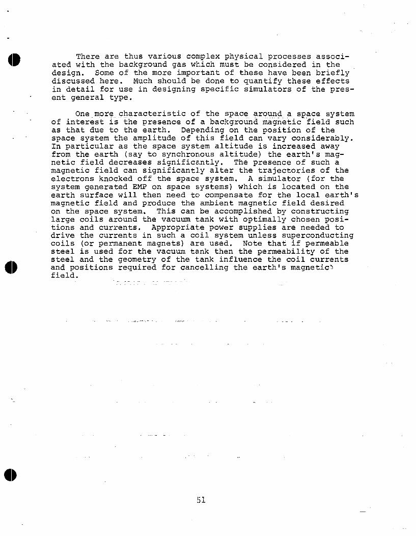
.
(B There are thus various complex physical processes associ-ated with the background gas which must be considered in thedesign. Some of the more important of these have been brieflydiscussed here. Much should be done to quantify these effectsin detail for use in designing specific simulators of the pres-
. ent general type.
One more characterist<c_of the space around a space systemof interest is the presence of a background ma”gnetic field suchas that due tc the earth. Depending on the position of thespace system the amplitude of this field can vary considerably.In particular as the space system altitude is increased awayfrom the earth (say to synchronous altitude) the earth’s mag-netic field decreases significantly. The presence of such amagnetic field can significantly alter the trajectories of theelectrons kno.cke.d..o.fft.h.e..spacesystem. A simulator (for thesystem generated EM? on space systems) which is located on theearth surface will then need to compensate for the local earth’smagnetic field and produce the ambient magnetic field desiredon the space system. This can be accomplished by constructinglarge coils around the vacuum tank with optimally chosen posi-tions and currents. APProFN~@te power supplies are needed todrive the currents in such a coil system unless superconductingcoils (or permanent magnets) are used. Note that if permeablesteel is used for the vacuum tank then the permeability of thesteel and the geometryand positions requiredfield.
of the tank influence the coil currentsfor canceling the earthls magnetic’>
!;1
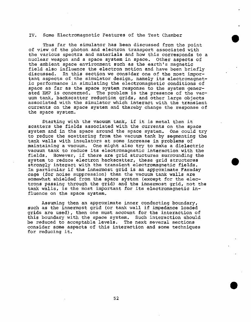
.
.
Iv. Some Electromagnetic Features of the Test Chamber
Thus far the simulator has been discussed from the pointof view of the photon and electron transport associated withthe various spectra and materials and how this corresponds to anuclear weapon and a space system in space. Other aspects ofthe ambient space environment such as the earth’s magneticfield also influence the electron motion and have been brieflydiscussed. In this section we consider one of the most impor-tant aspects of the simulator design, namely its electromagnet-ic performance in simulating the electromagnetic conditions ofspace as far as the space system response to the system gener-ated EMP is concerned. The problem is the presence of the vac-uum tank, backscatter reduction grids, and other large objectsassociated with the simulator which interact with the transientcurrents on the space system and thereby change the response ofthe space system.
Starting with the vacuum tank, if it is metal then itscatters the fields associated with the currents on the spacesystem and in the space around the space system. One could tryto reduce the scattering from the vacuum tank by segmenting thetank walls with insulators at some increase in problems ofmaintaining a vacuum. One might also try to make a dielectricvacuum tank to reduce its electromagnetic interaction with thefields. However, if there are grid structures surrounding thesystem to reduce electron backscatter, these grid structuresstrongly interact with the transient electromagnetic fields.In particular if the innermost grid is an approximate Faradaycage (for noise suppression) then the vacuum tank walls aresomewhat shielded from the space system (except for the elec-trons passing through the grid) and the innermost grid, not thetank walls, is the most important for its electromagnetic in-fluence on the space system.
Assuming then an approximate inner conducting boundary,such as the innermost grid (or tank wall if impedance loadedgrids are used), then one must account for the interaction ofthis boundary with the space system. Such interaction shouldbe reduced to acceptable levels. ‘Thenext several sectionsconsider some aspects of this interaction and some techniquesfor reducing it.
52
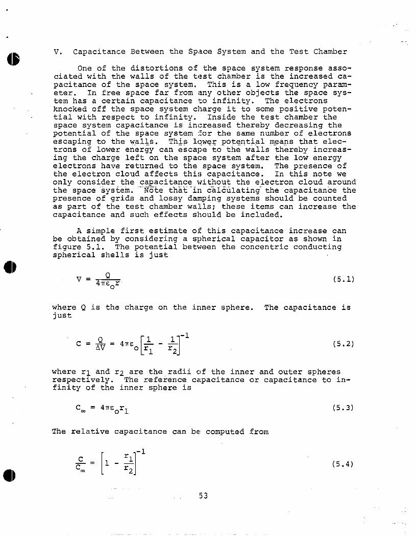
v. Capacitance Between the Space System and the Test Chamber
One of the distortions of the space system response asso-ciated with the walls of the test chamber is the increased ca-pacitance of the space system. This is a low frequency param-eter. In free space far from any other objects the space sys-tem has a certain capacitance to infinity. The electronsknocked off the space system charge it to some positive poten-tial with respect to infinity. Inside the test chamber thespace system capacitance is increased thereby decreasing thepotential of the space system for the same number of electronsescaping to the walls. This lqwer potential means that elec-tro-nsof lower energy can escape to the walls thereby increas-ing the charge left on the space system after the low energyelectrons have returned to the space system. The presence ofthe electron cloud affects this capacitance. In this note weonly consider the capacitance without the electron cloud aroundthe space system. Note t-hai-incalculating’ the capacitance thepresence of grids and lossy damping systems should be countedas part of the test chamber walls; these items can increase thecapacitance and such effects should be included.
A simple first estimate of this capacitance increase canbe obtained by considering a spherical capacitor as shown infigure 5.1. The potential between the concentric conductingspherical shells is just
Qv=—4meor
where Q is the charge on the inner sphere.just
c Q
[1
11-1‘E=4~&oq-q
(5.,1)
The capacitance is
(5.2)
where rl and r2 are the radii cjfthe inner and outer spheresrespectively. The reference capacitance or capacitance to in-finity of the inner sphere is
The relative capacitance can be computed from
[1-1
c ‘1—=cm l-—
‘2
(5.3)
(5.4)
53
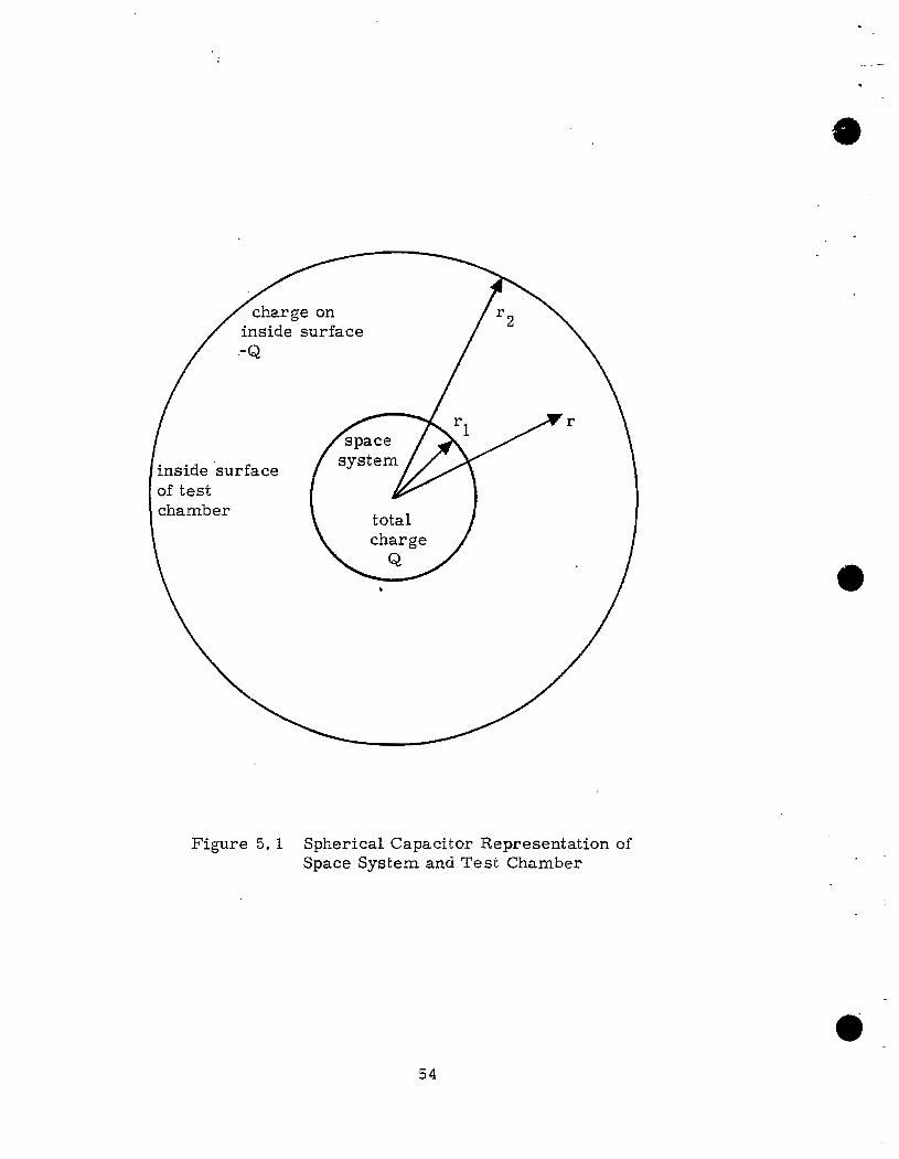
.
—
.
insidesurfaceOftestchamber
Figure 5,1 SphericalCapacitorRepresentationofSpace System and ll?estChamber
54

.
,
9P The relative capacitance increase
[1-1
ACc-C~=lrl—=cm cm -F--’ 1
2
[1-1,
‘121-7 ==‘2 2
which for rl/r2 + O is
2AC ‘1
(( ))‘1—=—
C. . r2 ‘o ~
is
[1-1
‘2 ~—-‘1
(5.5)
(5.6)
This relative capacitance increase is one figure of merit forthis type of simulator; it should be kept small compared to 1.
The relative capacitance increase can be calculated forvarious shapes of space systems and inner chamber walls (in-cluding grids and damping structures) . A useful approach tothis problem is to approximately separate the space system ge-ometry from the chamber geometry. To do this one can defineeffective values of rl and r2 from two separate electrostaticboundary value problems. Consider the space system with somenet charge in free space and calculate Cm, its capacitance toinfinity. Use this to define #
c;-
‘1 ‘~ (5.7)eff
This is a special type of mean radius for the space system.
As one goes farther away from a charged space system infree space the equipotentials are approximate spheres. Findingthe best fit for the center of these approximate spheres in thelimit of large rad~us for the equipotential surfaces defines anelectrical center rcl for the sl?acesystem. The electricalcenter can also be equivalently defined from
; =“Jspace (5.8)
55
●
where p(~) is the charge density on $he system. Note then thatfor a coordinate system centered on rc~ the system has no elec-tric dipole moment. The leading term in the potential andelectric field expansion comes from the electric monopole mo-ment (or total charge) given by
Q=.1 P(:)dV (5*9)spacesystern
The position of the electrical center of the space system issometimes cbvious from the symmetry of the space system or ofthe idealized shape representing it.
Having reduced the space system to an effective radius andan effective center let us do something similar for the testchamber. Assuming that the space system is very small comparedto the inner test chamber dimensions (including grids, dampingsystems, etc.) then replace the space system by an arbitrarilysmall charged sphere of radius ro. Move this test sphere in-side the test chamber until its capacitance to the test chamberis minim~zed. Find the limit of this position as r. + 0. Thisdefines rc2r the electrical center of the test chamber. Insome cases of test chamber geometries the position of this min-imum may not be unique and/or there may be relative minima inthe test volume. However such cases are not very useful fortest chamber design if one wishes to test only one space systemat a time.
Having found the electrical center ~c2 of the test chamberone can then find the effective radius r2eff for the insid$ ofthe test chamber. With the small test sphere centered on rc2calculate the capacitance and use
(5.10)
which comes by replacing rl by r. and r2 by rz f in equation4.2 and then taking the+limiting case of a smaf$ test sphere.Note that the position rc~ of minimum capacitance for the smalltest sphere is that position which maximizes r2eff.
In calculating r2eff one must include the various equip-ment attached to the inside of the tank walls. This includesthe grids for electron capture and the electromagnetic dampingsystem which may be also sparse like a grid so as to emit fewelectrons in the photon and electron environment incident on it.The innermost of these sparse structures is the most important
56

.
,
0 for determining r2eff. As a first rough estimate of r2eff onecould simply choose an average radius from the geometric centerof the test chamber (assuminf,~appropriate symmetry) to the in-nermost conducting (even fin~tely conducting) materials whichwould be placed inside the vacuum tank connected to the tankwalls through various impedances, etc. Since these structuresare somewhat sparse then r2e~.fis somewhat larger than an esti,-mate which assumes these strictures a conducting surface at theinnermost position. The actual r2eff is increased and theextra distance can be estimated for grid like structures using
.’ various boundary value problems such as for two dimensionalgrids.16
By use of the technique of spherical inversion the inter-ior boundary value problem fc)rr2eff can be converted into anexterior boundary value ~robl.emin which the arbitrarily smalltest sphere centered on rc2 is converted into an arbitrarilylar~e sphere approaching infinity.17 The inversion is centeredon rc2. By this procedure the calculation of r2e$f is con-verted into a calculation for rleff (with appropriate conver-sion factors) with a somewhat.altered shape. One can thenchoose an appropriate geometry (such as an ellipsoid) for theinverted exterior geometry and invert it back to an interiorproblem of interest so_a_sto tabulate r~eff for various inter-ior chamber shapes.
For the exterior problem such as used for calculatingrleff, the effective radius of a space system, there are manyshapes that one could consider and tabulate. One of the sim-pler of these is the ellipsoid which has a closed form solutionin terms of an elliptic integral.17 An ellipsoid with three‘separateprincipal-axis radii,gives some flexibility in tryingto approximate objects of interest. By using such a shape toenclose a space system of interest one can obtain an upperbound on rleff. Such a shape inscribed inside the outer bound-aries of a space system (if conducting) can be used to obtain alower bound on rleff. An average of upper and lower bounds canbe used as an approximation of rleff.
This low frequency capacitance between the space systemand the test chamber is one of the definable parameters for theinteraction of the two. There are various detailed boundaryvalue proble~s to be+solved and tabulated for rleff and r2eff(as well as rcl and rc2 in some cases). Various geometriessuch as ellipsoids, el~iptic cylinders, rectangular parallele-pipeds, etc. can be considered. For cases that the internaltest chamber dimensions are not much larger than the externalspace system dimensions then the problem does not quite splitinto a separate consideration of the space system and testchamber parameters as outlined above. Such more complex mutualinteraction problems can also be considered. Many specificboundary value problems need to be considered in detail to def-
,)initively understand this type of system-simulator interaction.
57

.
One effect of the capacitance increase is to allow moreelectrons toreach the cavity walls than would escape to infin-ity from an object in free space. The potential between thespace system and the cavity walls is also less than the poten-tial to infinity for the same object in free space. This ef-fect can be partially compensated by giving the space system aninitial positive charge. This charge can be introduced througha high value resistor string (with small cross section) from apower supply connected to the innermost electron trapping grid(and damping structure) or to the tank wall. The resistorstring would have large enough resistance that no significantcurrent can flow through it during times of interest for thesimulated system generated EMP. This technique has a drawback,however, in that it alters the electron trajectories outsidethe space system at early times during the pulse, whereas astate of no initial charge would give a more realistic simula-tion at early times. Of course, one could test the space sys-tem with various different initial charges in the same simula-tor. After tests this charging system can also be used to dis-charge the space system.
Part of the charge (negative) that escapes to the tankwalls should ideally return to the space system (if it were inspace) at some time characteristic of the round trip time ofelectrons of less than, but near, the energy of the electronsthat escape from the space system. One might do this throughresistive paths to the space system, but this would have thesignificant disadvantage of only returning these electrons tochosen discrete positions on the space system conductors. Fur-thermore such resistive paths would complicate the design ofeither or both the equipment for placing an initial charge onthe satellite and the paths for returning electrons to thespace system. One could better place electron guns at variouspositions around the tank wall (or on the innermost electrontrapping grid) to reintroduce electrons with an appropriateslowed down waveform and at appropriate energies.
Note that capacitance increase is only an approximate wayto characterize the increase in electron loss to the tank wall.In the presence of space charge the capacitance changes. Thusone can define a capacitance change under space charge limitedconditions. Such calculations would be a helpful addition tothe usual capacitance calculations. However in the real trans-ient situation such a steady state calculation with spacecharge will not be accurate either.
58

.
.
96 VI ● General Considerations for the Use of Discrete LoadingAntennas on the Wall of the Test Chamber
Now move to somewhat higher frequencies, frequencies suchthat the associated wavelengths are of the order of the dimen-sions of the internal vacuum chamber dimensions. In such afrequency range a cavity is resonant at various discrete fre-quencies if the cavity is lossless. Among other problems to beconsidered the cavity resonances excited by the electronsemitted from the space system (and other sources such as thephoton generator, electrons from the walls, etc.) need to beconsidered. These resonances should be damped to improve thesimulation at late times (compared to the characteristic timesassociated with the cavity size). There are various detaileddesigns for the damping system one might use. However, allthese designs must have the characteristic of not greatly in-terfering with the desired electromagnetic characteristics ofthe cavity at other significant frequencies, such as with thecapacitance reduction at low frequencies or with the reflectionreduction (from the cavity walls, damping structures, etc.) athigher frequencies. There are many desirable performance char-acteristics for the type of simulator under discussion. Theoptimum simulator design for ~3ivensimulator and space systemsizes is one which takes all of these performance features intc)account and compromises .~ong them so as _toobtain the best
4)
overall performance and minimizes the “errors” associated withthe simulator across the entire frequency band of interest.What is best in one frequency band may be incompatible withgood performance in other frequency bands and would then bediscarded in favor of other approaches.
One way to introduce loss into the cavity resonances is bythe addition of small electric and magnetic dipole antennaswith lossy impedance loading onto the cavity walls. Thesewould be placed so that the electric antennas would couple tothe cavity modes at positions where the electric field perpen-dicular to the cavity wall is large. Similarly the magneticantennas would be placed so that they are coupled to large mag-netic fields tangential to the cavity wall. These types ofdamping structures are indicated in figure 6.1 for single elec-tric and magnetic dipole antennas as well as combinations ofthese. Note that for any one location on the cavity wall (in-nermost grid for electron trapping) there are three field comp-onents of interest associated with the cavity modes, one elec-’tric and two magnetic. Correspondingly there are one electricand two magnetic dipole moment components of interest that canbe induced in loading antennas on the cavity wall. For thelower order cavity modes with antennas small compared to thecavity dimensions the antennas can be considered electricallysmall. Va.riou.snotes deal.with the characteristics of suchelectrically small antennasO-18~19
59
L
%27-/.
77779%7electric
m“,electricand magnetic
(onlyone magneticcomponent)
Only one mode is
degenerateso thatmore loadsareneeded toalsodamp therotationsofthismode.There are alsomany othermode patterns.
shown here. This istheEl,Ior TM1, ~mode. This mode is
6 s
magnetic
A, Generaltypesofloading
.“
zL4
z‘5
electricand magnetic(twoorthogonalmagneticcomponents)
antennas
@is theangleoftheprojectionofr on thexy planefrom thepositivex axis.
r
Yexample oftwo loading
v ‘osi’ions
. —
o
.
B. Loadingdipolesatdiscretepositionsinsidea sphericalcavity-
Figure 6,1 DiscreteLoadingon Cavitywalls
60

.
.
0 The load impedances (ZL in figure 6.1A) on the electricallysmall dipole antennas can have various characteristics. Theymight be frequency independent resistances. They could also bean inductor plus a resistor on the electric antennas or a ca-pacitor plus a resistor on the magnetic antennas. The elementvalues could be chosen to make the antenna with its loading im-pedance resonant at some desired frequency such as a cavityresonance frequency and thereby increase the damping of thatcavity resonance if the resistance is optimally chosen. Adamped cavity mode, however, has a complex resonance frequencyand this prevents a lossy rescmant coupler from attaining anarbitrarily large rate of energy extraction from the cavityfields. Using active devices in the load impedance one canperhaps increase the damping coefficient, but at a cost of com-plexity. Certainly it would be good to do some detailed calcu-lations for such small loading antennas with various types ofimpedances. However, there is a fundamental problem with smallan-tennas-which leads to low damping efficiencies, namely theantennas are small leading to small coupling to the cavityfields. One can avoid this problem by making large distributed.coupling structures as will be discussed later.
Another problem with resonant damping structures is that,there is not only one mode to damp. There are many cavitymodes (including degenerate modes) to damp. This leads to manyresonant frequencies for even the lower order modes that onewould consider in.the response of such a cavity to a ratherbroadband EMP. It is not sufficient to damp only one mode.This requires that the individual damping antennas operate atmany discrete frequencies or be broadband enough to cover thesame frequency band, or that the various modes be damped byseparate damping antennas thereby leading to a large number ofsuch damping antennas.
One of the disadvantages of using discrete damping anten-nas on the cavity wall is mode conversion. If one determinesthe cavity modes and resonant frequencies for an unloaded cav-ity and then introduces a disc:reteload not only are the var-ious re-sonancesshifted but the original modes are coupled to-gether. Equivalently this can be considered as shifting themode distributions over the inner cavity surface. As an exan-ple the spherical symmetry of a spherical cavity is destroyedby the introduction of discrete damping antennas so that theindividual spherical vector wave functions do not give the re-sulting natural modes of the cavity with damper(s) . If thereis only a little damping of the cavity modes due to smallcoupling to the small loading antennas, then the damping anten-nas can be considered as perturbations in using the undampedcavity modes. However, small damping is not what is wanted fora good simulator.
One would like the resonances to damp out in say a cycleor less. Thinking of the damped resonances as complex resonant
61

.
—
frequencies, then damping corresponds to moving poles off theiu axis (s = Q + i.ubeing the complex frequency plane) so thatthe magnitude of the real part of s at the pole in the left halfplane is of the order of (or larger than) the magnitude of theassociated imaginary part of s. If Sa = Qa + iua is the reso-nant (or natural) frequency then Qa (or -Oa) is what is referredto as the damping constant. One would like to minimize lua/!_lalfor each resonance Sa of concern.
If one wishes to damp many low order cavity modes usingdiscrete small loading antennas then many antenna positions areneeded. This results from the many mode patterns for the vari-ous resonances and the resulting variation among the modes ofthe positions on the cavity wall for maximum coupling and forthe positions of nulls. To illustrate some of these problemsconsider the spherical cavity as illustrated in figure 6.lB.In this figure only the mode with smallest resonant frequencyis shown; this is the E~,l or TM1 ~ mode. One can couple intothis mode where the magnetic fiel~ is maximum or where theelectric field is maximum as shown in figure 6.lB. However,this mode is degenerate and can be rotated through any angleabout the coordinate center. One can find three independentorientations for this mode with say the electric field maximum(magnetic field null) positioned on the x, y and z axes to de-fine the linearly independent modes. TO couple to the electricfield maxima of the three modes requires at least three elec-tric dipole antenna dampers; for coupling to the magnetic fieldmaxima requires at least two magnetic dipole damper positionswith two magnetic dipole components for the loading antennasused at one of these positions (or magnetic dipole loading atmore positions) .
As one goes to higher order modes for a sphere the degen-eracy is more severe requiring more discrete damping antennasfor the higher order modes. The modes for the s herical cavity
5arise from the spherical wave functions given by O
f(k)(yr)Yn,m,a(6,@)~(~) (y:) = n‘n,m,a
f(~)(yr)= f(fi)’(yr)Pn,m,a(O,@) + n Yr dn,m,a(O,$)n
62

.
+-($)
IM,CJYZ)= vx W:,(Y‘y;)](6.1)
The spherical harmonics are
Y e(e,$) =/
P:(coS (e)) ~cOs@$’) ~~sin (MO) =0, 1, 2, ““*nrmro
3SI,rn,a(e’$)= ‘syn,rn,o(e’o) = ‘r x %,m,o(g’o)
3 e(e,$) = 36n,nt,o
where the index a stands for esubscriptfunctions
is a unit vector forare
(even) or o (odd) and ~ with athat coordinate. The Legendre
63

,
—-
.
P:(E) = (-l)m(l
Pn(G} = P“(g) =
The spherical Bessel functions are
. .
n1)
denoted by f~$~(yr) where
(6.3)
.’
f(l)(yr)n = in(yr) = injn(kr)
(6.4)
f(2) (yr) = kn(yr) = i-n-2h~2) (kr)n
where the propagation constant is
where the psrmittivity s, permeability I-L,and conductivity adepend on the specific uniform, isotropic medium under consid-eration. Ot
??fforms of spherical Bessel functions such as
yn(kr) and h (kr) can also be used as convenient. The spher- 0ical Bessel !?unctionscan be calculated from
(6.6)
A prime superscript on a spherical Bessel function indicatesthe derivative with respect to the argument. Solutions of Max-well’s equations caribe constructed in spherical coordinates bylinear combinations 0$ these wave functions. For solutionswithout sources only M and N functions are needed for thefields as
64
,
.
0
which hasas giving
‘1,1
which can
(6.7)
where a tilde - indicates the Laplace transform and where thewave impedance is
“m (6.8)
Solutions for the interior modes of a perfectly conductingsphere are found by setting L = 1 (to constrain that the fieldsbe well behaved at r= O) and by constraining that the tangen-tial electric field be zero cm the spherical surface r = a.There are two types of modes, The En,n! or TMnfnl modes arebased on the electric field in terms of * functions; the Hn,nl
ff~g$;~ns.modes are based on the electric field in terms of
The E1,I mode in figure 6.lB is associated withn= landm= 1 in the fifunctions. The resonant frequenciesfor the E modes are found from
[un,n,in(un,n,)]’ = O
which has the first few zero:; ([oin(o)l‘ being excluded) at
%,10 z i2.744, ‘2,1(,= i3.870 (6.10)
which can be set equal to ya to obtain the resonant frequency,,The H mode resonant frequencies are found from
in(v ,) = Onfn(6.l:L)
the first few zeros (the zero at in(o) being exc~ud~~didentically zero fields) at
s +J4.493 ,‘2,1 = &i5.763 (6.12)
be set equal to ya to obtain the resonant frequencies.
65
.
. .
The mode functions on a spherical surface are vectorsphe$ical harmonics. The normal electric field appl es only tothe N vector wav~ functions and is contained ih the $ sphericalharmonics. The M type electric fields have no radial electricfield and so electric loading antennas on the cavity wall donot apply for Hn,n~ (o$ TEn,n’) modes. The tangential magneticfiel~ is given by the R spherical harmonics for E modes and bythe Q spherical harmonics for H modes. One can consider thepatterns of the fields at r = a and some texts have a few plotsof this for various modes.21 For the higher order modes thesepatterns on r = a become rather complex with many sign rever-sals for the various field components. Correspondingly theyare highly degenerate and a linear combination of such degener-ate modes (for a single resonant frequency Sa) forms a “new”mode with shifted null positions (many of them) for a particu-lar field component. For discrete damping antennas enough an-tenna positions are needed for each Sa to couple to all the de-generate modes so that there is no combination which givesnulls for the appropriate field component at all the positionsof the coupling antennas for that Sa.
As a convenient example the spherical cavity is being con-sidered in this note. However, one might distort this geometrysomewhat in a real simulator of the type presented by this note.This will remove some or all of the mode degeneracy and splitthe associated resonant frequency into several such resonantfrequencies. This cavity distortion still leaves one with manymodes and more resonant frequencies to damp. One should also onote that the presence of the space system in the test chamberwill also alter the resonant frequencies and modal distribu-tions and each different shape and size of space system willalter these somewhat differently. Thus the optimum positionsand impedances associated with resonant dampers can change be-tween tests, thereby complicating matters.
In order to quantify the attainable damping for the vari-ous modes using discrete damping antennas on the cavity wallsthere need to be some detailed boundary value problems workedout; these are beyond the scope of the present note but willhopefully be done in the future. From the present discussion,however, it is clear that there are significant disadvantagesin this technique. These disadvantages are removed somewhat bythe use of continuous damping structures as are discussed next.The continuous damping structures at least have the advantagesof being large and thereby coupling more efficiently to themodes, as well as coupling to most or all of the cavity modes.The use of a large number of discrete damping antennas becomesa continuous damping structure in the limit of an infinitelylarge number of damping antennas. One might note that somecombination of discrete and continuous damping structures mayalso be useful butto determine their
such designs requireadvantages, if any.
66
de~ailed calculation=
.
.
e VII. Impedance Loaded Shell Inside Cavity and Away from theWall for Damping Cavity Resonances
Let us go on to consider simple continuous damping struc-tures. With an assumed spher~.calcavity of radius r = a as in-dicated in figure 7.1 let us include a spherically symmetricdamping structure inside the perfectly conducting surface atr a. This use of spherical symmetry in the damping structureke=ps the mode distribution unchanged with respect to f3and $;
the ,rdependence of the modes is changed in general, however.
Consider a spherical shell of radius r = b and sheet im-pedance 2s as an example of a continuous damping structure asshown in figure 7.1. The cavity parameters are those of freespace with
(7.1.)
With Zs/Zo and b/a as parameters (although Zs may be frequencydependent) one may consider the damping of the cavity modes.
First consider the E modes which have the form for O z r ‘:b as
E( p(l);(:,s) = &fn,m,a(Y:)
o
and for b < r < a as
Ei(z,s) =
{
+(1)&M ‘(2) (y:)}o 1 n,mra(yz) + a2Mn,m,a
(7*:))
(7.:3)
Constraining the tangential electric field at r = a to be zerogives
67

o
Cr=o“p
impedanceconductor
z~
Figure 7.1 Impedance Loaded ShellforDampingCavityResonances
68
...

.
*
o ~l[yain(ya) 1‘ + a2[Yakn(ya) 1‘ = O
and constraining thethrough r = b gives
(7.4)
tangential electric field to be continuous
(al - l)[ybin(yb)]’ + a2[ybkn(yb)]’ = O (7.5)
The surface current density on the surface r = b is,-
3+($,s) = +5(:,s) (7=6)s
r=b
and the tangential magnetic field is discontinuous through r = baccording to
This gives another equation for the coefficients as
[ybin(yb)]’~{ (al - l)in(yb) + a2kn(yb)] =o yb
For convenience we have the Wronskians
w{in(~),kn(c)} = in(~)k;(~) - i:(c)kn(~) = -L-2
W{~in(L),Lkn(G)} = Lin(q)[Ckn(g)l ’ - [Cin(L)l’Ckn(C) = -1.
Let us combine equations 7.5 i~nd7.8. First substitute foral - 1 giving
z‘a2{-ybin(yb) [ybkn(yb)l’ + [ybin(yb)l’ybkn(yb)}Z.
= {[ybin(yb)l ’}2
(7.7)
(7.10)
which reduces to
69

.
= >{ [ybin(yb)]‘]2a2 ~, (7.11) oNext substitute for a2 giving
>(CL1- 1) {ybin(yb)[ybkn(yb)]’ - [ybin(yb)]’ybkn(yb)}o
= [ybkn(yb)]’[ybin(yb)]’ (7.12)
which reduces to
- >[ybkn(yb) l’[ybin(yb)l’%=1 ~
Combining equations 7.4, 7.11, and 7.13 then gives
/
[yain(ya)]’ 1 - #[ybkn(yb) l’[ybin(yb)1’s }
+ [yakn(ya)l’>{ [ybin(yb)l’}2 = Os
(7.13)
(7.14)
.
Note for 2s = @ so that the damper is removed this result re-duces to
[yain(ya)]’ = O , [kajn(ka)]’ = O (7.15)
as required for a lossless spherical cavity. For 2s = O it re-duces to
[ybin(yb)]’ = O (or [kbjn(kb))r = O)
(7.16)
[yain(ya)]’[ybkn(yb)]’ - [yakn(ya)]’[ybin(yb)]’ = O
the first of these giving the interior resonances for a sphereof radius b and the second giving the resonances between twospherical shells (perfectly conducting) of radii b and a.
●70
>
.4
4B
.
Let
and rewrite equation 7.14 as
(7.17)
[yain(ya)]’{zs - [ybkn(yb)]’[ybin(yb)]’}
+ [yakn(ya)l‘{[ybin(yb)]’}2 = o (7.18)
Now if ya = un,n~ is a solution for zs + @ and/or b + a (bothof which give a cavity of radius a) then the shifted resonancecan be written as un,n~ + Aun,nr or u + A for short. Note that(with zero excluded)
[u ,i (Un,n,)]’ = On,no no
(7.19)
Then expand the various,d/a and small frequency
noting that
yb =(u+A)~=(u
functions in a Taylor series for smallshift A where
(7.20)
+A)(l- $)=u+A-~u-~A (7.21)
Then equation 7.18 can be expanded for small d/a and A as
1A[uin(u)]” + $[uin(u)] ‘“ + ()(A3)I
/{“z-
S [uJcn(u)l’+O(A-& -:A)~
.[[A-~u ]-~A [uin(u)]’’+O((A-~u-= ‘A)2)~
1
71
,.,
1+ [ukn(u)]’+O(A-$$*-gu
0~{[ a. 1-~A 2{[Uin(U)]”]2
.-
= 0 (7.22)
Retaining only up through second order terms we have
A[uin(u)]’rzs+ ;[uin(u)lf”z~[
-A A-~u-$1A {[uin(u)]r’}2[ukn(u)l’
[ 1
2+ A-~u- ~A {[uin(u)]’’}2[ukn(u)]’
= 0(A3)+O(A2(A-~u-~A)) +O(@u-$&]2)+0([A-@~A]3)
(7.23)
which can be shortened as
A2A[uin(u)]”z~ + ~[uin(u)]’” z~
i-[
du--a 1[ 1-~A A-~u-~A {[Uin(U) ]’r}2[tdCn(U)]’
=0 (7.24)
Now neglect the A2 terms compared to A and neglect the (d/a)Aterms with respect to d/a or A to obtain the approximation
(7.25}
as the equation for the change in natural frequency for smalld/a but any zs. In another form we write this out more explic-itly as
72
.
0
.
(Aun,n ‘)~zs-~ ‘n,n~[un,n~in(un,n~) ]’’[un,n~kn‘“n,n~ \)],/
+ [~un,n~[un,n:in(un,n:)lff[un,n:kn(un,n:)l1 ‘o (7.2~)
from which AUn,nI can be readily solved in terms of d/a and zs.The un,n: for the unloaded cavity are found for the first fewmodes (equations 6.10) as
‘1, 10= i2.744~
U1,20= i6.117
‘2, 10z i3.870 ,
‘2, 20z i7.443
(7.27)
‘3,10= i4.973,
‘3,20c i.8.722
The approximate relation of Aun n’ to zs and d/a can nowbe determined for the lower order mo~es. Note that as zs + OJwe have Aun,nl + O as is required physically. Also as zs + Owe have Aun,nl + (d/a)un,n& which is also quite reasonable as asimple perturbation on the cavity radius from a to b. Onewould like to be able to choose an optimum zs for any given d/a.An optimum zs requires a definition of the optimum Aun,nl. Letus adopt as our definition of an optimum natural frequency onewhich has the maximum argument in the second quadrant of thecomplex frequency plane. This maximizes lQal/\ual for the com-plex frequency. For small Aun,n~, since un,n~ (unperturbed) isa pure imaginary number, the definition is approximately thesame as minimizing Re[Aun,n~] .
Now zs can be complex if one chooses. If one requiresthat it be realizable from passive elements then it is re-stricted somewhat. For the p:resentlet us make zs a real andpositive number corresponding to a simple resistive shell.Write an equation for Aun,nl as well as for its real part as
Aun,n,
u= -($n,nr[zs - :an,n, }-l
n,n~u
ct:an,n’ =U n,n~[unrn~in(un,n~)]’’[un,n~kn(un,n’)]’o
73

.
.
Differeritiati~g”with respect to zs and factoring gives
or
or
(7.29)
(7.30)
(7.31)
.-
so that the optimum value for resistive zs is
I(7.32)
which is a rather simple result with the optimum resistive zsdirectly proportional to d/a. Substituting this result back
into equations 7.28 we have the small Aun,nl resulting from
optimum resistive 2s as
dAun,n, = ‘u l~;,nla n,no
1~ct ,1jl-1=~-+
(%’ = -an,nt{~an,nll - an,nl}n,n~ n,n’ 1
(7.33)
74

-.
@
T
/a\2-a a .lIi= -Im[an *2/ay - (a+w=z 2 t
Thus for the optimum resistive zs theproportional to d/a.
!Imn, n,l
frequency
Starting with the differential equation
-Re[an,n,l}-1
shift is also
(7*34)
then we can write
U2 +n(n+l)n,n~a u
=
n,n’ u u ,irl(un,n’ n,no n,n~) ‘Un,n$kn(un,nl)]‘
o 0 0(7.35:)
From a Wronskian (equations 7.9) we have
a =-n,n’
U:,n ,+n(ni-1)0unrn;
(7.36)- n(n+l)= -un,n; u-n,n’
0
since [<in(~)]’ = O at ~ = Un,n&. Thus ~n,nl is pure imaginary.
The result for a’ can be further simplified. Consider thespherical Bessel functions. We have the relations
h(2) (~)n = jn(g) - iyn(~)
(7.37)
75
.
.
By considering the small argument asymptotic formso
in(~) = ~2n::), ,[l+o(G31 , kn(c) = ~-n-l(2n-l)!![l+ O(~)]..
jn(~) = En
. .
~2n+1)1![l+o(G2)l , Yn(g) = -&-n-1 (2n-l)!![l+O(~2)]
.
h(l) (~) = -ig-n-l (2rI-l)!![l+ o(&)] ,n
(7.38)
h(2) (g) = i~-n-ln (2n-l)!![l+ O(&)]
oneFor
can find the signs of the functions for small arguments.convenience we also have (to complement equations 6.6)
m
h(l)(g) = i-n-lg-l eigz (n+@)! -Bn 8! (n- ~)!(-izg)
@=o
so that
m
“-n-2kn(+= 1
gives the appropriate functions for incoming waves.
Now letting
(7.40)
(7.39)
u = ipn~n~ - n,n’ (7.41)
we have
76

-..an,n’
=U nrn~[un~n$n-(un ~n~)‘-”‘Un,n;kn‘Un,n’)]‘o
= -Pn,n’[pn,n’]n(pn, n’)] ’’[pn,n’hA2)(pn,nl)]’
= ip.,n,n’ [pn,n,jn(pn,n,)ll’[pn,n,Yn(Pn,n,)1’
(7.42)
since
[pn,n,jn,n, (pn,n,)l’ = O (7.43)
defines the roots pn,nl (= -i~~n,n~)for the unloaded cavity.All the pn,nl are real (the un,n’ being imaginary) as is re-quired for a lossless cavity. T~e jn(~) and yn(~) are realfunctions for real & (or imaginary C) as well as all their de-rivatives. Therefore an,nl must be purely imaginary as ob-served above.
As discussed in another note20 the zeros of spherical Bes-sel functions fn(~) and combinations like ~fn(~) and their de-rivatives have only simple zeros for c # O. Thus
[Pn,n ,jn(pn,n,)l” # O
and from a Wronskian one can also show (equations 7.9)
[Pn,nlYn(Pn,n!H ‘ + o
(7.44)
(7.45)
so that
an,n’ + 0(7.46)
Now the zeros of [pn,nljn(pn,n!)]” alternate between thosefor [pn,nljn(pn,nt)]’ and so the sign of [pnrnljn(pn,nl)]” al-ternates between adjacent roots pn,n~ as n’ 1s varied. When[&jn(g)l’ changes sign (at its zeros) then [~yn(g)l’ cannot
,change.sign.(from the Wronskian) nor can ~jn(~) change sign(from the differential equation); the same argument appliesaround the zeros of other similar combinations of three terms.Consider two adjacent zeros of [ jn(~)]’ which we denote by PIand p“. Write out the Wronskian 5
w{Ejn(C),~yn (E)l=~jn($) [EYn(~)l’- [gjn(&)l’Eyn(g) = 1 (7*47)
77

.
At the endpoints of our interval
(7.48)
Since jn(&) has opposite sign at the two ends p,p’ then so must ‘[&Yn(&)l’. Thus [&yn(~)]’ must have at least one zero betweenp and p’. Considering two adjacent zeros of [~yn(~)]‘ a simi-
.-
lar argument shows that [Ejn(?)]’ must have at least one zeroin this new interval. Combining the two results shows that thezeros of [&jn(E)]’ and [Eyn(c)]~ must alternate on the real Eaxis (neglecting ~ = 0). Thus the sign Of [pn,n~yn(pn,nl)]’must alternate for adjacent roots (successive n’). Since theexpression for C%nn! has a product of two terms with alternat-ing signs then lm~an.n~l must have the same siqn for all n’(for any given n).
--,-.Considering the result for-aq,nf for large
un,n~ for which it is negative imaginary for positive w givesfor all n,n’ (which are indexed
Re[an,n,] = O , Im[an,n,]
Using this result for an,n~
~1
n,n’ = [l-il-l=*
for positive u)
<o (7.49)
in equations 7.33 gives
(7.50)
which holds for all n,n’ corresponding to the roots pn,n~ .Thus for optimum choice of zs (which does depend on n,n’) wehave for small d/a the result
Aul+id=— .
n,n’ 2 a ‘n,n~ = + :Iun,n, ~a
(7.51)
with real part negative and imaginary and real part positive asrequired physically where only positive pn,nl have been consid-ered. For negative pn,nl the imaginary part is negative.
As examples and to obtain a few numbers we tabulate thefirst several anrnt as
al,l = -i2.015 ,alr2 = -i 5.790
a2,1 =-i2.320 ,
a2r2 =-i 6.637
(7.52)
a3,1 =-i.2.561 ~
a3,2 =-i 7.346
78

@Considering the El,l mode for d/a = .1 we have
,29(5z~ =“gm,”
*’J1,l’U1,10 = .05 + i .05
and for d/a = .2 we have
.&f3~.nzs ‘ R?(I’15, AUl,l/Ul,Lo = .1 + i.1
(7.53)
(7.54)
Equation 7.51 readily extends these results to other E modeswith optimum choices of resistive zs for the individual modes.
Second consider the H modes which have the form forO’<r<bas
Eo+(l)ii(i?,s)= -TN
o n,m,a (y&)
and for b < r < a as
(7.55)
“’ (7.56)
Constraining the tangential electric field at r = b to be zerogives
Blin(ya) + 62kn(ya) = O (7.57)
and constraining the tangential electric field to be continuousthrough r = b gives
(61- l)in(yb) + f32kn(yb)= O (7.58)-
The surface current density on the surface r = b is

andr =
3J6,+,S) = +W,s)s r=b
.
(7.59)9
the tangential magnetic field is discontinuous throughb according to
+er X {fi(~ts)IK=b+ - ‘(zrs)lr=b-} = ‘s(e!+rs) (7.60) -
This gives another equation for the coefficients as
z
[
[ybin(yb)lr [ybkn(yb)]’
~ (61-1) Yb + 62}=,in(yb) (7.61)
oyb
,
Combine equations 7.58 and 7.61. First substitute for
61 - 1 giving
~f3{-[ybin(yb)l’ybkn(yb) + Win(yb)[ybkn(yb)]’}02
= {ybin(yb)}’
which a Wronskian relation (equations 7.9) reduces to
s’ = ->{ybin(yb)}’s
(7.62)
(7.63)
Next substitute fOr 62 giVin9
Zs~(e~ -l) {[ybin(yb)l’ybkn(yb) -Ybin(yb) [ybkn(yb)l’}o
= Ybkn(yb)ybin(yb) (7.64)
which reduces to
%=2+ >ybkn(yb)ybin(yb)
s
80
I

.
.—
0 Combining equations 7.57, 7.63, and 7.65 then gives
Iin(ya) 1 + >ybkn(yb)ybi,n (yb)I
s J
Z.- kn(ya) ~{ybin(yb)};~ = o
s
Note for Zs = m so that the damperduces to
in(ya) = O , jn(ka) = Cl
(7.66)
is removed this result re-
(7.67)
as required for a lossless spherical cavity.duces to
For 2s = O it re-
in(yb) = O (or jn(kb) = O)
(7.68)
ink -kn(ya)in(yb) = O
the first of these giving the interior resonances for a sphereof radius b and the second giving the resonances between twospherical shells (perfectly conducting) of radii b and a.
Equation 7.66 can be rewritten as
yain(ya){zs+
- yakn(ya)
ybkn (yb)ybin (yb)}
{ybin(yb)}2 = o
Expand this solutionya + = so that
in(v ,) =0n,no
with zero excluded.
(7.69)
around vn~n~ which is a solution for
(7.70)
Then expand the various functions in aTaylor series for small d/a and small frequency shift A. Notethat

(7.71)
where v is short for vn,nl and A for Avn,nl . Then expand equa-tion 7.69 for small d/a and A as
[
2A[vin(v)]’ + ~[vin(v)]’’+0(A3)
}
.[ Jzs+/vkn(v)+O(A-$;A)\
-1vkn(v) +OIA-$.@ A))
= o (7.72)
Retaining only up through second order terms we have
A[vin(v)] ‘zs+ $[vin(v)][
“zs+A @V-1
:A {[vin(v)]’}2vkn(v)
[ 1
2- A-;v- ~A {[vin(v)]’}2vkn(v)
= 0(A3) +O(A2[A-~V-~A)) +O(AIA-~V-~A)2)
which can be shortened as
.
.-
0’-
(7.73)
82
.
.
(D A[vin(v)] ‘z~+ ~[vin(v)l”z~
[
+d ~v+1[
:A A-$T-1
~A {[vin(v)]’}2vkn (v)
Now neglect A2 with respectspect to d/a or A to obtain
‘z.+: v[A-:vl’vin(v)’
or
(7.74)
t.oA and neglect (d/a)A with re-the approximation
‘vkn(v) = O (7.75)
(Avn,n‘){zs+~vn,n~ ‘vn,n~in,n’(vn,n~)]’vn,n~kn ‘vn,n~)1
- [:vnln:r’vnrn;in?n:(vnrn’)l’vntn:kn(vn?n:)‘0 ‘7”7’)
from which Avn,n! can be solved in terms of d/a and zs. Thevn,n~ for the unloaded cavity are found for the first few modes(equations 6.12) as
V1,10 = i4.493, ‘1,2C)= i7.725
‘2,10u i5.763, v2,2a
z i9.095 (7.77)
‘3,10E i6.988, ‘3,20
= i10.417
The approximate relation of Avn,n~ to zs and d/a can nowbe determined for the lower c)rdermodes. Note for zs + @ thatAvn,n’ + O. As zs + O we have Avn,nt + (d/a)vn,n& consistentwith the results for the E mades. Again let us consider anoptimum zs for any given d/a based on minimizing Re[Avn,n’] forsmall Avn,nl as before.
Let zs be a real and positive number corresponding to asimple frequency independent resistive shell. Then we canwrite
83
.

.
~5f3 =n,n~[vn,n~in(vn,n~)]‘Vn,n;kn(vnrn;)-v
n,n’ -
Forthe
and
the H modes this equation is of theE modes (equations 7.28) giving the
2s = :li3 1n,n’
a resulting frequency shift as
(7.78)
same form as that foroptimum resistive zs as
(7.79)
dAvn,n, = –v ~’a n,n~ nln’
(7.80)
These results are the same as those for the E modesferent constants in the formulae.
From a Wronskian (equations 7.9) we can write
t3 = -vn,n’ n,n~
with dif-
(7.81)
since Vn,n&in(Vnrn~) = O at ~ = un,n~o Thus Sn nl is pureimaginary. Considering only the roots for positive w then we ‘have
Re[~n,n,] = O , Im[8n,n,] < 0
Using this result for ~~,n’ in equations 7.80 gives
(7.82)
.-
084
\

o B:,n, = [l-i]-l = * (7.83)
which holds for all n,n’ (n = 1, 2, 3, .... n! = l.,2, 3, ...).For small d/a then we have (with optimum z~)
Av ~l+i~v =n,n’ 2 a n,n~ + $vn,n, I
o(7.84)
Note that
— .—
so that both E and H modes have the same optimum damping forsmall d/a. The values for optimum zs vary depending on n,n’and on whether E or H modes are being considered.
Considering the Hl,l mode for d/a = .1 we have
.yY~3zs =.*,
*V1,l’V1,10 = .05 + i.05
and for d/a = .2 we have
$q~.
zs = i49.3 ,
%,lh,l =.1+i.1o
(7.86)
(7.87)
Equation 7.84 readily extends these results to other H modeswith optimum choices of resistive zs for the individual modes.
A rather interesting result is that both Aunfnl/un,n~ andAv t/vn,n~ have the same form with zs scaling with ~n,nl and~n~~~ in the two cases respecizively. For a given small d/a thetrajectories of Au and Av are the same in the normalized com-plex frequency plane as zs is varied. Another interesting re-sult for these trajectories, taking Au as an example, is foundfrom equations 7.28 as
85
.
.
a ‘sld~~+l=-- -2aaz~ (7.88)
.— -du~
For resistive zs with un,n& an the positive imaginary axis thisresult leads to
(7.89)
so that the trajectories of Aun,nr and Avn,nr are circles inthe normalized complex frequent
7plane for resistive zs and
small d/a with radii (1/2)(d/a) un,n~l and (1/2)(d/a)~vn,nlIrespectively.
Note that the simple results only apply for small d/a withfrequency bounded. As one goes to higher order resonant modesthen d/a must be made smaller so that it is still small com-pared to a (complex) radian wavelength. The value of d/a canbe such as to place the resistive damper at a null of the tan-gential electric field of a given resonant mode and thus giveno damping for that mode. One can find such unwanted values ofd/a, or equivalently b/a, for the lower order modes by choosingtwo values of n’ for a given n and given E or H mode and con-sidering the ratios
ub n,n~—=au n,n~
where n“!> n“ >modes are -
or
vb n,n~—=av
n,n;’!o
1. Some of these
(7.90)
ratios for the lower order
86

.
0
.
‘1, 10 ‘2,10 ‘3,10— = .449 , — =!.520 , — s .570‘1,20 ‘2,20 ‘3,20
(7.91)
‘1, 10
‘1,20.582 ?
‘2, 10
‘2, 20.634
‘3,10— E .671‘3,2 o
For small d/a (or b/a near 1) these critical values can beavoided for the lower order modes. As one goes to higher fre-quencies then for small d/a one will get no damping if d is aninteger number of half wavelengths for imaginary s (= iu).This points’out a general limitation on the effectiveness of aresistive sheet damper for reducing reflections of the higherfrequencies (say from space system resonances) from the cavitywalls. The damping structure can be made of more than oneshell, however, or given some thickness as a liner which isconsidered in the next sectio:nfor comparison.
Note that Zs can have forms other than a simple resistance,but one must be careful because this damping and reflection re-duction structure has to perform well for many modes and over alarge frequency band. Simply concentrating on damping one res”-onant mode (say the lowest frequency one, the El,l mode) doesnot lead to an optimum simulator design. However, other inter--esting forms of Zs, including reactive elements, need furtherconsideration in future notes from the viewpoint of making thedamping structure more effect~Lvelybroadband.
Another task left for a future note is a detailed numeri-cal study of the mode damping for arbitrary b/a (in the range Oto 1) from equations 7.18 and 7.69 for resistive Z.Swith()< Zs < @c These equations also are the starting point forcofiside~ingother forms of zs. Note that the approximate poleshifts considered in this section are for small shifts from theundamped modes with resonant frequencies on the iu axis. Otherpoles may arise in the left half of the complex frequency planewith various forms of passive damping structures and these canalso be found and their behavior studied. Additional indiceson the poles (beyond n,n’) may be useful in such cases.
87

.
.
VIII . ImpedaticeLoaded Liner Inside Cavity and in Contactwith the Wall for Damping Cavity Resonances
As illustrated in figure 8.1 let the region for b < r c abe a uniform’isotropic medium with constitutive parameters e,p, a, wave impedance Z, and propagation constant y. The mediumfor O < r < b has the parameters of free space which can bedistin~uished by a subscript O (including on 20 and ye).
Consider first the E’modes which have the form for(l:r<bas
Eo+(~)if(i?,s)= TMo n,m,a (yo:)
and for b < r z a as
(8.1)
(8.2)
Constraining the tangential electric field at r = a to be zerogives
~l[Yain(Ya)l ’ + a2[yakn(ya)l~ = o (8.3)
At r = b both tangential electric and magnetic fields must becontinuous~ thereby
[ybin(yb)]‘
al yb
giving
[ybkn(yb)]‘+ C%2
yb
[Yobin(Yab)1‘=
‘ob
(8.4)
alin(yb) + a2kn(yb) = ~in(yob)o
From these equations first eliminate al to give
88

.
.
0
perfectconductor
Figure 8.1 Impedance Loaded Liner in ContactwithCavityWall forDamping Resonances

.
~2{@in (Ybl[Ybkn(Yb)1 ‘ - [ybin(yb)]‘ybkn(yb)}
= (yb)2 .~ln(yb) [Yabin(Yob)l~ - $Yb[ybin(yb) 1‘in(yob) (8.5)o 0
which a Wronskian relationship reduces to,,
(yb)2 .a2 = -~~n(yb) [yobin(yob)l‘+ $yb[ybin(yb) l’in(yob)
o 0(8.6)
. .
Next eliminate a2 to give
al{[ybin(yb)l’ybkn(yb) - ybin(yb) [ybkn(yb)]’}
which reduces to
(yb)2“k (Yb)[Yobin(yob)]‘- Z.al = yob n
~yb[ybkn(yb) ]’in(yob] (8.8)
Note that if the parameters of the linerinner cavity then a2 = O and al = 1 (thefrom a Wronskian relation) .
are the same as thelatter result coming
Combining equations 8.3, 8.6, and 8.8 gives
[[yain(ya)]‘ ybkn(yb) [yobin(yob)]‘- $-[ybkn(yb)]‘yobin(yob)~
o
+ [yakn(ya}l’~-ybin(yb) [yobin(yob)l’+!
$[ybin(yb) l’yobin[yob)fo
= o (8.9)
For y = y. and Z = 20 so that the damper is removed this resultreduces to
90
.
0[yoain(yoa)]’ = O
as required. For a + ~ with fixed s, p, and s we have
=
Consider
-1@iF{l + O(cr-%
(8.10)
(8.11.)
the asymptotic forms of the spherical Bessel functionsfor large arguments as for IGI + ~ with larg(~)l ~ 7r/2- 6 with6>00 From equations 6.6 we have
~in(~) = e;~[1 + O(G-1)1
-3[1 + o(~-l):l~kn(~) = e
e~[~in(~)]’ = ~[1 + O(~-:L)]
[Zkn(C)I’ = -e-L[l + O(K-L)]
For IGI + @ with larg(~)l = ~/2 we have
-~][1 + o(~-1)]Gin(G) = +[ec + (-l)n+L e
-C[l + ()(~-l)jLkn(L) = e
-L] [1 + o(~-1)][Gin(C)l’ = ~[eC + (-1)11e
[Gkn(G)l’ = -e-G[l + O(U-l)]
Define
(8.1;!)
(8.13)
91

.
(8.14)
and rewrite equation 8.9 as
[yain(ya)]’{ybkn(yb) [yobin(yob)]’-zl[ybkn(yb) ]’yobin(yob)} . .
+ [yakn(ya)l’{-ybin(yb) [yobin(yob)l’+zk[ybin (yb)l’yobin(yob)1
= o {8.15)
Now let y +~ (from a + ~) with Iarg(y)l ~ m/2 - 6 with 6 > 0giving
~ya‘L)]{-e-yb[l+O((yb)-l)l [Y. ~ o~[1 -t-O((ya) bi (yb)l’
+Ze ‘yb[l+O((yb)k ‘1)lyobin(yob)}
‘ya[l+O((ya)1
eyb-e -1)1 -~[l+O((yb) ‘1)1[yobin(yob)1‘
eyb+ Zk ~[l+o((yb) -l)lyobin(yob)
1
= o (8.16)
Neglecting terms proportional to ey(b-a), but not those propor-tional to ey~a-b) (since a > b) gives
{-[yobin(yob)]f+ z~yobin(yob)}[1+0( (yb)-l)] =O(e-y(a-b)) (8.17]
Note that
Z,=<= @i&=$? (8.18)
so that as ]yl + w with Iyol bounded we have in the limit
92
,.
.
0 [yobin(yob)]’ = O (8.19)
as the equation for the E mode resonant frequencies correspond-ing to a perfectly conducting cavity of radius b.
As an.aid to considering the solution of equation 8.15 forsmall d/a consider first the effective impedance at r = b.Neglect the form of the fielc[sfor r < b for the moment andconsider the ratio of the tar~gential‘electric and magneticfields at r =b. For thisas
purpose equations 8.2 can-be written
&b /r=b[
\=Eon(n+l) a(1
in(yb).—
yb
1[ybin(yb)]‘
+al “ yb
(8.20)E#(:,S)/r=b = f{alin(yb) +a2kn(yb) }~n,m,a(O,@)
Then choosing ~ and ~ pola$itie$ suc8
that 3 x 3 is in the ~rdirection and ~oting+that R = -er x (so that the tangentialcomponents of E and H are simply related for all 0,$) then wehave an effective wave impedance at r = b as
[ybin(yb)]‘ [ybkn(yb)]‘
‘b al—+a
yb 2 yb‘bE~=- alin(yb) + a2kn(Yb)
(8.21)
Using equation 8.3 for the boundary condition at r = a gives
[yain(ya)]‘[ybkn(yb)]‘ - [yakn(ya)]‘[ybin(yb)]‘
‘b=- ~ - [yakn(ya)]‘ybin(yb) (8.22)
Using the relation
93

.
.
we can write far the impedance at r = b
(8.23) ‘
-[-yakn(-ya)]‘[Ybkn(yb)I ‘+ [yakn(ya)1‘i-ybkn(-yb)]‘ (8 24)
‘b = ~ ‘[-ybkn(-yb)l “
where a prime indicates the derivative with respect to the argu-ment (ya, -yar etc.) of the Bessel function.
For large /yal (and thus large lyb~ since d/a is taken asa constant (small)) we have
%=
=
-1 -%+ouyb)-l-ya[l+o((ya)-l)~ew[l+o((yb)-l
‘a[l+o((yal-e )le -+]% ‘L)]em[l+O((@)-l) 1
‘a[l+o((ya) ‘ya[l+O((ya)‘Yb[l+o((yb) )1-e-e ‘1)]e )1
e‘d[l+o((ya)‘l)]-e‘Ydil+o((ya)-1)1
eyd[l+O((ya)‘l)]+e‘ydIl+o((ya)-l)~(8.25)
If Ieyd +to
‘b =
e-ydl is bounded away from O then this result reduces
eyd - ~-ydd[l + O((ya) -1) 1
eyd + e-Y
l-e-2yd
I + e-2yd[1 + O((ya)-1)1
(8.26)
.
0
Note that for a plane wave incident perpendicular to a slab ofthickness d with a perfectly conducting backing this result isexact so the result is physically quite reasonable. Also note
that while Iyal is large for this estiimate Iydl need not belarge since d/a is small. For small Iydl this reduces to
94

.
.
0 %2=\d - ;(yd)3+0( (yd)5)~[l+O((Ya)Zb=z ,Y -1)1
= spd~l -~(yd) 2+o((yd) 4)\[l+o((Ya)‘b -1)1
For comparison consider the result for small Iyal.this we have
Ckn(c) = (2n - 1)!!c-n + o(~-n+~)
[Lk-(~)l’ = -n(2n -lL ,,
n-l-lGin(C) = (2nC+ 1)!!
(8.27)
For
(8.28).n+3
+ 0((, ).—
[~in(~)l’ = (2nn++l?j!! ‘nn+2
+ O(K )
From equation 8.22 we then have
‘b -n~~~~) (ya)n(yb)-n-l[l+O(ya)]+n~~~~) (ya)-n-l(yb)n[l+O(ya)l
%=T=- =( a ‘(yb)-ntl+o(ya)l+~(Ya)2ni-ly) ‘n-l(yb)n+l[l+o(Ya)1
-n n+l~ n(n+ l)(~) - n(n+ l)(~)’
=—yb -n n+l—[l+O(ya)]
(n+l)(~) + n(~)
1l+n~ -1+ (n+l)~= n(n+l)
+ 0({:]2)
yb
I(n+l)[l+n~]+ n[l-(n+l)~] + 0([$2) ‘l+O(ya’]
yb -++o(:)]u+o(Yw = ‘(::’):F+O(:)][l+o(Ya)J=n(n+l) d
‘b = :;;::] :[,+0(:)][l+o(ya)l= :;;;:)a :[1+0(:)][,+o(Ya)l
95

This result is quite different from that for large ]yal (but notnecessarily large Iyd/) in equations 8.27. Note that this re-sult is for E modes and for small ya the Bessel functions cor-respond to near fields of electric antennas with large E/Hratios. The result of equations 8.27 corresponds to the farfield form of the functions for which E\H is like the wave im-pedance of free space (before the perfectly conducting boundaryis introduced) .
In our case of interest lyoal is of order one, so ifIYl ‘~ IYol the results of equations 8.26 apply. The results ofequations 8.29 apply for small Iyal which requires even smaller~yoal so one is considering frequencies for which cavity reso-nances are not of concern, but capacitance is of concern (sec-tion V).
For convenience the equation for the cavity resonances canbe written for the E modes in terms of the impedance at r = b as
‘b [yobin(yob)]’—=-Z. yobin(yob)
or in terms of 21
‘b Z . “= - [yobin(yob)]’——z 20 = ‘bzk yobin(yob)
(8.30)
(8.31)
Now expand equation 8.31 around un,n~ which satisfies
[unrn,i (Un,n,)]’ = Oon o(8.32)
for which we have (as in the previous section)
yoa =U + Aun,n: n,n’
[1
(8.33)
yob =yoal-$ =U +Au ‘~un,n;
-~Aunrn’ a n,ng n,nf
Abbreviating these terms as u and A we have
96

>
For Zbing to
uin(u)
[uin (
‘A]3)~u)]’”+0 (A-$-=
(8.34)
let us use the approximation for large lyal (correspond-large o) without assuming the size of Iyd I. Also then
expand
ya
yd
z.X4
a
[s11(0+ SC)]1/2a = (spu)l/2a[l +0(0-1) ]
()
(y a)l/2 Uoa 1/2
o [1+ O(CJ-l)]
I/W
[ 1( )
1/2ul/2 l+~$+O(A2) ~ [1+0(0-1) ]
00
pyouyoad—— —— —Ho Y = P. @ a
=dpu+A.——a PO yd
combination for yd at the unperturbed resonances
(8.35)
as
97—-—
1/2
()
1/2r ~ Ydl~=~ = (sn,n,U(a+Sn,n,S})l’2d=(~) U1’2A [1+0(0-1)1
n,nt o 00 m
(8.36)
1Ayd-r= ~:r [l+o(a-l)]
Now expand
~2yd-2~ -e-2r[l+o(a-1)]: ;
u+A=~2yd-2~ +e21’ ~r+(yd-r) (8.37)
Dropping the O(a-~) terms for simplicity and expanding in terms-G A we haveU.L u
Then
Fromtion
= 1- e-2r d p ~+O(A)-—~+e-2r a P. r
we can write
l-e-2r d P u———~+e-2i7 apo r “ -[@~l
the differential equation
(8.38)
[uin(u)]“
Uln (u) (8.39)
for the spherical Bessel func-terms (equation 7.34) we have
98

.
,
(D
4)
[un,n
,in(un,n,)]” u~,n,+n(n+l)o 0 0=
u .,1 (un,no n n,n~)
Lun,n~
1 +n(n+l) =
.L
un,n’o
an,n’.—un,n~
(8.40)
where an.nl was introduced in the previous section (equation7.36). ‘-Thenwe have
Au
I
un,n’ ~ d
n,n’o P L l-e-2ru
~l+r—:-n,n~ n,n’ U. f l+e-2r 1
(8.41)
Note thatimpedance at r
this can also be written in terms of a general=bas
Aun,n’=~+l abun,n~
—qaan,n’
(8.42)“
where Zb is evaluated at the frequency corresponding to un nl .Note that this assumes lZb/Zol << 1 so that the change in heeffective wall’impedance from zero is sufficiently small thatthe shift in resonant frequency is also small and that IZbldoes not get too large at (or too near) this resonant frequency.There are various forms of Zb that one might choose so as tooptimize the shift of the resonant frequency. Equations 8.42show how much damping they achieve for small d/a (and smalllZb/Zol) with a somewhat simpler form than that in equation8.40.
In’using a form of Zb in equations 8.42 one should be care-ful that approximations for Zb are accurate. For example sec-tion VII considers the case of y = y. but with a surface imped-ance added at r = b. Such can be found from equation 8.24(with y = yo) with the parallel addition of 2s. In such a caseZb would be approximated by expanding yob as a small perturba-tion from yea. This would not give the simple form of resultfor Zb as in equation 8.26 since yoa is of the order of a con-stant (unless we consider the result for large n’ and thuslarge lUn,n&/). For the present we are considering lyl >> Iyolso that the result of equation 8.26 applies. Equation 8.41then gives the result for small d/a.
99

.
.
Now an,nI is negative imaginary (equation 7.49) for posi-tive imaginary un,n~ 9ivin9 o
u’nrn’-1<7 ‘~o
n,.n’(8.43)
In order to minimize the real ,part of Aunrnl we then need
Re [Au 1 ‘n,n;
[
-2rn,n’ = d ~m p n-e. —
\u a an,n~’ n,nr P. ~ 1 + e-2”r1
(8.44)
Let p be real (and typically equal Po). Then we need to mini-mize Im[v] where
For this purpose approximate
r = (s~((s + se))l/2d
1/2d[l + c)(c#) ]= (Sva)
= (spa)~/2d
= (&J’2dWith (sn,n~a)/c = un,n~ then we have
giving
(8.45)
(8.46)
(8.47)
oI.oo
.
@
—=l+ij sech2 (r) - 1
r{~tanh(I’)j
(8.48)
Since $ is real we wish to f~.ndr. such that
[nn sech2(ro)
1- +tanh(ro) = O
0(8.49)
with
r. = (1 + i)$o
(8.50)v =o ~L-tanh(ro)
o
The numerical solution to these equations is
!JO = 1.127
r. = 1.127 + il.127(8.51)
v’=o .582 - i.417
Figure 8.2 shows v plotted as a function of ~. Note that Im[v]has a single minimum and smoothly rises toward zero on bothsides of this minimum. Also note that Re[v] starts at 1 andmonotonically decays to zero as $ varies from O to CO.
Next then we define
un,n’Pn,n’ :l+aovo
n,n’(8.52)
101

.
01.0
.9
.8
●7
.6
.5
.4
.3
.2
.1
0
-*1
-.2
-.3
-.4
-,5
.
.
.
.
.
.
.
.
.
.
.
I I 1 I I t I
o 1 2 3 4 5 6 7 8
$
.
Figure8.2 FactorinlrnpedanceofLiner
102

–- .+ –=.–
has valueswhich for the various n,n’
W1 = .208 + i.568 , !J7*= .386 + i .441
~ .0297
s -.130
+ i .696 , .348
.309
find
+ i .468
+ i .495
the conductivity for
~2,2 (8.53)
+ i.810,‘3,2
Given a particular un,nl we canoptimum damping (with real p? from
(8.54)
or
(8.55)
frequency shift (for real U) isThe resulting resonant
Aun,n’un~n:
which for u = PO is
Aun,n,~d
u ~lln,n,n,n~
(8.57)
examples considerAsfor v =have
the conductivity and frequency shiftEll,lmode for d/a = .1 for which we‘JO. Consider the
103

aodzo = 9.260 , AyyJl,JQ = .0208 + i .0568 (8.58)
and for d/a = .2 for which we have
aodZo = 4.630 , Aul,liul,lo ‘ .0416 + i .1136 (8.59)
Equations 8.55 and 8.57 readily extend these results to other Emodes.
Compare the liner results (equations 8.53 and 8.57) forthe optimum damping for each E mode to the corresponding resultsfor the shell (equation 7.51). Note for the shell that themagnitude of the damping coefficient is .5(d/a)lul for smalld/a. However, for the liner the optimum damping is differentfor each mode and the magnitude of the damping coefficient isgreater than .5 for small n’ while it is less than .5 for largenF. For small n’ (say n’ = 1) also note that the damping isgreater for larger n. In all, the optimum damping with theliner is about the same as with the shell. For the lowestorder mode, the E~,~ mode, the liner gives a coefficient of.568, or about a 14% improvement (again for small d/a and p =Po).
Second consider the H modes which have the form forO~r<b
3(;,s) = o n,m,a(yoz)~ fi(l)
Eo+(1)fi(;,s)= -=No n,m,cf(yo~)
(8.60)
and for b < r < a as
I
+(1)ii(~,s)= E. S M
+(2) +)1 n,m,o (Y~) + @2Mn,m,a(yrlj
(8.61)
Constraining the tangential electric field at r’= a to be zerogives
~lin(ya) + f32kn(ya)= O (8.62)
.-‘*
-
104
—
#
At r = b both tangential electric and magneticcontinuous, thereby giving
[ybin(yb)]’.
‘1 + $2yb
Eliminating (31gives
62{ [ybin(yb)l’ybkn(yb) -
= in(yob)
fields must be
[ybkn(yb)]’ ~ [yobin(yob)]’
‘yb ‘~ yob
= [ybin(yb)]’ybin(yob)
which reduces”
i32 = [ybin(yb)
to
]‘ybin(yob)
ybin(yb) [ybkn(yb)]’}
.- Z (yb)4.
~ ~ln(Yb) [ybi (yob)]’n
Z (yb)2.1 (yb)[ybin(yob)l ’~ yob n
*
Eliminating 82 gives
Sl{ybin(yb) [ybkn(yb)l’ - [ybin(yb)]‘ybkn(yb)}
= [ybkn(yb)]’ybin(yob) - ~ ‘yb)2kZ. ~ n(yb)[Yobin(yob)]’
(8.64)
(8.65)
(8.66)
which reduces to
% =-[ybkn(yb) ]‘ybin(yob) + $ ~kn(yb) [yobin(yob)]‘
-.v w
Note that if the parameters of the linerinner cavity then-f32= OWronskian relation) .
Combining equations
and 61 = 1 (the
and
are the same aslatter due to a
(8.6’7)
the

.
~-[ybkn(yb)l’yobin(yob) + ~yain(ya)l z ybkn(yb) [yobin(yob)]”J
1+-yakn(ya) [ybin(yb)l’yobin(yob) - ~ ybin(yb) [yobin(yab)l’~
= o (8.68)
For y = y. and Z = Z. so that the damper is removed the resultreduces to
in(yoa) = O
as required. For o + ~ with fixed s, p, and s we can.useasymptotic forms of equations 8.11 through 8.13 to give
eya
~[l+O((ya)-l )l~e‘yb[l+O((yb) ‘1)]yobin(yob)
+zke ‘yb[l+O((yb) ‘1)][yobin(yob)1‘I
1
~yb+ e-ya[l+o((ya)-l)l ~[l+o((yb) -l)lyobin(yob)
~yb- zg~[l+O( (yb)-~)l[yobin(yob)l’~
.
(8.69)
the
9
= o (8.70)
Neglecting terms proportional to eY(b-a), but not those propor-tional to eY(a-b) gives in the limit
in(yob) = O (8.71)
as the equation for the H mode resonant frequencies correspond-ing to a perfectly conducting cavity of radius b. In terms ofthe normalized liner wave impedance ZI we have
,
106
●
o yain(ya) {-[ybkn(yb)l ’yobin(yob)+ziybkn (yb)[yobin(yob)l’}
+ yakn(ya){[ybin(yb)l ’yobin(yob) -zRybin(yb) [yobin(yob)l’}
(8.72)
This is the equation for determining the natural frequenciesfor the H modes for arbitrary d/a (with O : d/a : 1).
For the H modes the wave impedance at r = b can be foundfrom the fields there which are
3(2,s) E {Slin(yb) +~:lkn(yb)}~n,m,o(et$)r=b = o
(8.’73)
where again a prime “indicatesthe argument (yb, -yb) of the
E.
.{[
in(yb) kn(yb)
a(~,s) ~=b = -~ n(n+l) !31~+ ~2~
J [ybin(yb)I‘ [ybkn(yb)]’l~n,m,a(e,$lt
+ @l(
—+62yb yb f ~
Comparing $r X i to ~ and noting that ~r x ~ = b we have
~=-Slin(yb) +@2kn(yb)
‘bsz [ybin(yb)]’ [ybkn(yb)]’’61 Yb —+s2 yb
(8.”?4)
Using equation 8.62 for the boundary condition at r = a 9ive~s
yain(ya)ybkn(yb) -yakn(ya)Ybin(yb)1 (8.’75)
‘b = ‘yain(ya) [ybkn(yb)l’-yakn(ya) [yb~n(yb)l
Converting the in functions to kn functions from equations 8.23gives another form for the impedance at r = b as
- [-yakn(-ya)1[ybkn(yb)1 + [Yakn(ya)1[-ybkn(-yb)I(8.76)
‘b = [-yakn(-ya)1[ybkn(yb)1‘+ [yakn(ya)][-ybkn(-yb)] ‘
the derivative with respect toBessel function.
107
●
●
For large Iyal with small d/a we have
o
-eya[l+o((ya)~~)le-m[l+o((ybj-11] ~‘w[l+O((yb)-l)]+e-ya[l+O((ya)-L)]eW[l+O((yb)-~]]
‘b= -e‘a[l+O((ya) )Ie - ‘ya[l+O((ya)-l)]eW[l+O((yb)‘1)]
.‘yd[~+o((ya)~~)1eyd[l+O((ya)-l)]-e= (8.77)‘yd[l+o((ya) 11‘d[l+O((ya)-l)]+ee
If leYd +duces to
‘b =
which ismodes;
For
e-Ydl is bounded away from zero then this result re-
+ o((ya)-~)l
l-e -2yd
~ + e-2yd[1 + O((ya)-L) 1 (8.78)
the same result (equations 8.26 and 8.27) as for the E
small !Ya! the normalized impedance at r = b reduces(from equation 8~75) to
‘b A( a- 2rl+ly) ‘+l(yb)-n[l+O(ya)1-+(ya~-n(yb)n+~ ‘1+‘(Y’)]
%=T=-+( an+l(yb)-n-l[l+O(ya)]-~(ya) ‘n(yb)n[l+O(ya)Jan-i-ly)
-n-l
(:) -[y=yb-n-1 ~[l+O(ya)]
n(:) +(ni-1)(~)
11+- (n+l)~-
}
l+n~+o(F]2)= yb
[ al+(n+l)~-n:]+o((:) z) ’l+o(y~)lnl+(n+l)~
(8.79)

*
.
0 ‘b= s~b~
[[l+o(~]][l+o(ya)]=svd l+o(~]][l+o(ya)]
Note th.a.t_the_re.suit...fo~ sm.al_l__Iya I differs from that for largeIyal. For small lyal the H modes have Zb inductive while the Emodes (equations 8.29) have Zb conductive and capacitive (inparallel). This result is quite similar to that for large Iyalin equation “8.78,particularly if /ydl is small for which wehave
‘b= yd[l + O(yd)][l + O((ya)-1)1 (8.80)
This result for the H modes is quite different than that forthe E modes. Note that the E modes differ from the H modes inthat the E modes have large radial electric fields near thecavity wall (or damper).
As in the case of the E modes let Iyoal be of order one(bounded above and below) with Iy I >> Iy. I so that the resultof equation 8.78 applies for the H modes. In terms of a gen-eral impedance at r = b the equation for the cavity resonancescan be Mitten for the H modes as
‘b ‘b Zyobin(yob)
—= .—Z. z Z. = ‘bzi = - [yobin(yob)]’
Expand this equation around vn,n~ which satisfies
in (v )0=n,n~
(8.81)
(8.82)
for which we have
yoa ‘v + Avn,n~ n,n’
‘(8.8.3)
yob[1
- tiv -d=yoa l-$ “v + AV
n,n’ nln’ a n,n~ ~Avn, n,o
Abbreviating these terms as u and A we have
109

.
(8.84)
where the second derivative term in the denominator is zero be-cause of the differential equation (equation 7.34). .
The results of equations 8.35 through 8.38 for Zb can becarried over for the H mode case with v replacing u giving
Then we can write
_-++jl-e-2rdpv~+e-2rapoI’
*For a general impedance at r = b we have
Avnrn,~g- 1 ‘b
v —qavn,n~ n,n~
o
(8.85)
(8.86)
(8.87)
o
For the special impedance form in equation 8.85 we have
Avn,n, ~d
[
-2r+p-= 1
vn,nr 0’ 1 + e-zr!o
(8.88). .
110
,=o

-“
{P
where v has been considered in equations 8.45 through 8.51.The minimum real part of Av is found at r = r. for which v = VooFor p = PO the optimum Av for small d/a is then found from
Avn,n,
v = @ - Vo] = [.418 +n,n~
u
which is conveniently independent
i .417]: (8.8!2)
of n,n’ for the relative fre-quency shift. Note that the damping coefficient magnitude is.417(d/a)lvl. This is less damping under optimum choice of athan is achieved for the_E mode damping for small d/a. For theH modes the”li”nergives less damping than the shell (equation7.84) for which the magnitude of the damping coefficient forsmall d/a and p = P. is .5(d/a)Ivl.
The optimum choice of liner conductivity is found fromequation 8.55 with u replaced by v giving
.
As examples considerfor p = PO. Consider the
P.
lJ2.541
~o
(8.90)
the conductivity, and frequency shift:H~,l mode for d/a = .1 giving
crodzo= 5.654 , ‘v~,@~,lo ‘ ●0418 +
and for d/a = .2 giving
Equations 8.89 and 8.90 readily extend thesemodes.
The results for small dla for the linerply only for frequency low enough or d smallsmall compared to a radian wavelength. Note
i .0417 (8.91,)
i .8345 (8.92)
results to other H
of thickness d ap-enough that d isthat the liner
cannot be-placed at a position of ~ero electric field for anunperturbed mode since the liner has finite thickness. In thisrespect the liner is superior to the sheet considered in sectionVII. The liner can be used to give a more uniform reflectioncoefficient for high frequency waves incident on the cavitywall from inside the cavity. This is considered further in thenext section.
111
The liner parameters E, P, a can have various more comp~exforms if desired. Again, however, one should be careful tochoose these parameters to give good mode damping over a largerange of frequencies corresponding to many modes. This ques-tion needs further detailed study.
A future note will hopefully numerically study the modedamping characteristics for arbitrary b/a from equations 8.15and 8.72. Various forms of s, p, and a can then be considered.One must also be concerned with the realizability of these pa-rameters using three dimensional arrays of lumped elements.There is some advantage in also using only passive elements insuch an array.
112.
..

.
.
s
.
IX.
well
Impedance Loaded Liner Inside Cavity and in Contact with-——=
the Wall for Reducing High Frequency Reflections
Having considered the resonances-of the test chamber asas sheet and liner dampers for damping these resonances
let us consider this phenomenon from another viewpoint, that ofreflections from the cavity wall (including sheets, liners,etc.). Cavity resonances correspond to a combination of out-ward and inward propagating waves which are related to eachother such that the fields are well behaved at r = O (satisfyMaxwell’s equations with no singularity there).
With a ,space system in the test chamber as indicated infigure 9.1 the cavity modes are changed. Some of the reso-nances are associated with the resonances (natural frequencies)of the space system. The reflections from the walls of thetest chamber alter the natural frequencies of the space system.A convenient way to consider the reduction of the effect of thecavity walls on the space system resonances is to minimize thereflection coefficients of the outgoing waves from the spacesystem at the cavity walls.
Considering a spherical.test chamber with a space systemat the center of the test chamber, let us represent the fieldsradiated from the space system in terms of outward propagatingspherical waves and consider the reflection coefficients forconverting the outward propagating waves into inward propagati-ng waves. This does not include the nonlinear effects associ-ated with the electron cloud which extends out toward the chamb-er walls. It is a limited,,but useful, view of the problem.
Since the space system ideally has linear dimensions smallcompared to 2b, then the radian wavelengths corresponding toresonances of the space system are also small compared to b.The cavity resonances without the space system present are alsoclosely spaced between resonances, in the sense that lAs/sl issmall between adjacent resonances for large resonant frequen-ties Isl for which there are many wavelengths across the cavity.As the natural frequenciessideration of a continuoustion from the cavity wallsof reflection reduction isquencies.
becoma closer together then a con- -frequency dependence of the reflec-is more significant. The viewpointthen most appropriate at high fre-
Consider first the E waves (those with a radial componentof the electric field) for O < r < b as
113
.

*
.
system generatingwaves which propagatetoward cavitywall
Figurefor
Representthisregionby electricand magneticdipoles@ and =)and otherhigherorder terms, o(Thereisalsoa monopole termassociatedwithnet charge.)
9.1 Impedance Loaded Liner in ContactwithCavityWaUReductionofReflectionofWaves Back Toward theSpace System
114

.
(9.1)
where the -yo~ argument indicates the incoming wave and re is areflection coefficient for the E waves. Note that at r = b thereflection coefficient can be written somewhat differently sothat it can be directly related to the impedance Zb consideredin the previous section. Nc}tethat in the definition of thespherical vector wave functions (equations 6.1) the kn(-yor)functions can be used, but the functions fn(yr) and their de-rivatives use yr as the argument. In the case of kn(-yor) itis convenient to shift the derivatives to those with respect to-yr so that derivatives are with respect to the argument of theBessel function.
Equating the rati~ of ~angential electric and magneticfields at r = b (with er x il= -~) gives
[yobkn(yob)]‘ [-yobkn(-yob)]‘+ re
~= yob yob
20 ‘bz~ = - kn(yb) + rekn(-yb)
[yobkn(yob)]‘ + re[-yobkn(-yob) ]‘=-
yobkn(yob) - re[-yobkn(-yob)l (9.2)
where the primes indicate derivatives with respect to the Bes-sel function argument, yb ox -yb in this case. Solving for regives
‘b[yobkn(yob)1‘ + ~ yobkn (yob)
r o=-e ‘b[-yobkn(-yob)]‘ - @-yobkn (-yob)]
o
(9.3)
From section VIII the appropriate impedance for the linerplus perfectly conducting wall, Zb, is given by equations 8.22and 8.24 for E waves. Note that the propagation constant inthis case is y instead of y. so that the net result is rathercomplex. Note for CJ+ ~ (large Re[y]) with s = iu that Zb + O.With Zb = O we have
115

.
.
r =-e
[yobkn(yab)]’
[ynbkw(-yAb)]{u Al u
corresponding to a perfectly conducting wall at r = b.s = iu and notj.ng.that
11
then on the
r =-e
lrel =
fL
imaginary frequency axis for Zb = (1we have
[ikobkn(i.kob)]‘
[ikobkn(ikob}]‘
1
(9.4)
For
(9.5)
(9.6)
\
Similarly if yo = y so that there is no added liner onecan substitute from equation 8.24 and obtain
[yobkn(yob)]’
‘e=- [-yobkn(-yob)]‘ (9.7)
which also has magnitude 1 on the iu axis. Note that re couldbe defined so that for a + ~ one would have re + -I.rtherebyreferencing the reflection coefficient to r = b. This would beaccomplished by replacing re by re[-yobkn(-yob)l’/[yobkn (yobll~in equations 9.2 and 9.3. Suppose then we define
[-yobkn(-yob)l’Pe ❑ re [yobkn(yob)l‘
(9.8)
This removes the phase delay from r = O to r = b and back andis convenient to use in some cases.
For small Iyobl the reflection coefficient reduces to
._
116

r =e
.=
Pe =
-n(yob)‘b‘n-l[l +O(yob)] + ~(yob)-n[l +O(yob) 10
“
-n (-yob)‘b‘n-l[l +O(yob) ] - ~(-yob)-n[l +O(yob) 1
u
(-l)n(l + O(yob) 1
(-l)n+l[l +
-1 + O(yob)
O(yob)lre
Note thatsmall [Sl
this assumes fixed o > 0 so that small Iyobl impliesand thus a constant non zero Zb from equations 8.29.
For large lyobl the reflection coefficient reduces to
re
yob ‘b-yob
-e [1 + O((yob)-l)] + ye [1 + O((yob)-l)]o (9.10)=-
yob ‘b -yob-e [1 +O((yob)-l)l - ~e [1 + O((yob)-l)]
Referenced to r = b we have
For large
Pe =
w
(9.11)
l-yo [-yobkn(-yob)1‘
Iyob I this is
1- ‘b~[1 + O((yob)-l)lo.
1+ ‘b@ + O((yob)-l}]u
117
17
.
‘b - ‘OZb -1-Z. (9.I.2)
This last result i.sexactly what one would expect for a planewave normally incident on a plane stratified structure with animpedance Zb at its front (input) surface. This last form willbe-later us~d with the high frequency form of Zb in order todiscuss minimizing Pe in a broadband sense.
Consider next the H wavesof the magnetic field) for O <
3(;,s) =0/ n,m,a(yo:) +
~ jfi(2)
Equatingatr=b
(9.13)
{
Eo +(2)ii(:,s)= -r Nn,mra(yot)
o
the ratio o$6
tangential electric and magnetic fields(with er X = ) gives
‘bkn(yob) + rhkn(-yob)
~ = ‘bzL = - [yobkn(yob)l’ [-yobkn(-yob)]‘+ rh
yob yob
yobkn(yob) - rh[-Yobkn(-Yob)]=-
[yobkn(yob)]‘ + rh [-yobkn(-yob)]‘(9.14)
Solving for rh gives
(9.15)
For a + @ (large Re[y]) with s = iu there results Zb + O.With Zb = O we have
,–
0118
.
[
‘h =
,yobkn(yob)
[-ynbk=(-y-b)1 (9.16)w lL u
corresponding to a perfectly conducting wall at r = b. Fors = iu and noting the conjugate symmetry of the kn functions
‘h =
lr~l
ikobkn(ikob )
[-ikobkn(-ikob)]
Similarly if yo = y so that there is nocan substitute from equation 8.76 and obtain
yoakn(yoa)
‘h = [-yoakn(-yea)]
which also has magnitude 1the reflection to r = b by
‘h
Ph
(9.17)
liner one
(9.18)
on the iu axis. One can reference
[-yobkn(-yob)]Phs-rhybky
on(o b)
For small Iyobl the reflection coefficient
(yob) ‘b‘n[l+O(yob)] - ~n(yob) -n-l[l+o(yob)]n
‘b-(-yob)-n[l+O(yob)] -- ~n(-yob) -n-l[l+o(yob)]o
(-l)n[l +O(yob) ]
(-1)n+l [l+ O(yob)]rh
-1 + O(yob)
(9.19)
to
(9.20)
119
Note that this assumes thatsmall then Zb from equationsling one of the yob terms in
For large lyobl the refl
yal is also small. If d/a is also8.79 is proportional to s cancel-the above expression for rh.
ection coefficient ,reduces to
-yob ‘b -yobe [l+O((yob)-l)] - ~e [l+o((yob)-~)l
o‘h = - yob (9.21)
-e [1 +O((yob) -l] -Zb yob~e [1+O((yob) -l)]o
Referenced to r = b we have
Ph
‘b [yobkn(yob)1‘,1+7
o Yobk~(yab)
‘bk--‘b [-YO n{-yob)]‘l-~
o[-yobkn(-yob)]
For large ~yobl this is
1- ‘b@ + O((yob)-l)l
ph=- 0
‘b1.+ ~[1 + O((yob)-l]]o
‘b - ‘O
‘b + ‘O
This result is the same as that forthe result for a plane wave normallyified structure with an impedance Zbface.
~e for largeincident onat its fron
IYOWa plane
t (input)
(9.22)
(9.23)
It isstrat-sur-
For small d/a with a uniform liner with large Iyal (im-plied by large ~yob[) equations 8.26 and 8.78 give for both Eand H waves
.—
Ii’
.
120
‘b—=Z.
for largeincludingfor large
‘b Z Z1-e -2yd——z Z. = ‘bzi = ~~ + e-zyd (9.24)
IYa I ‘hich is 9~~nl ~:a~everal alternative ~ondition~,large s, p, a, The reflection coefficient
E and H wives isIYoal for both,
‘bl-ro“ (9.25]
Consider some cases to obtain a proximate forms for thereflection coefficients. TFirst let yod~p/po << 1 with YO
u real. Let G :>> ls~~ so that weand
~dz
‘bq’
with
v
r
+
P
(9.26)
=(1+
real.
i) (~) 1’2d
Then we have
1- + yodvo
1+ $ yodvo
2\
(~w) )-L+; 2yodv+0 (
o
(9.27)
121
.
..
With y d positive imaginary the magnitude of p is minimized forsmall 71yod by minimizing the imaginary part of v. As consid-ered in section VIII (equations 8.44 through 8.51) for which wehave the optimum choice of $, I’,and v as
r. = 1.127 + i.1.127
v = .582 - i.417o
For a given frequency onefrom equations 9.26. Thecient is
(9.28)
can choose an optimum conductivitymagnitude of the reflection coeffi-
IP] = 1 + 2~lyod]nn[vl (9.29)‘o
which for optimum choice of conductivity gives
IPI =1- .834~PO
This shows that until
yod 1 (9.30)
yod]~/po approaches 1 only small reduc-tions of the reflection coefficient are achievable. Larcreu/urnlowers the frequency for which a certain reduction of lp~ is-‘-achievable but the most interesting case has B = MO since thereflection reduction (damping) structure should be sparse toavoid photon and electron collisions thereby precluding largevolumes of magnetic materials.
‘Now let lyod~ ~> 1 so that we also have Iydl >> 1, atleast on the iu axis. Let a << ~s[s so that we have
(9.31)
.-
●▼
,
122
.=
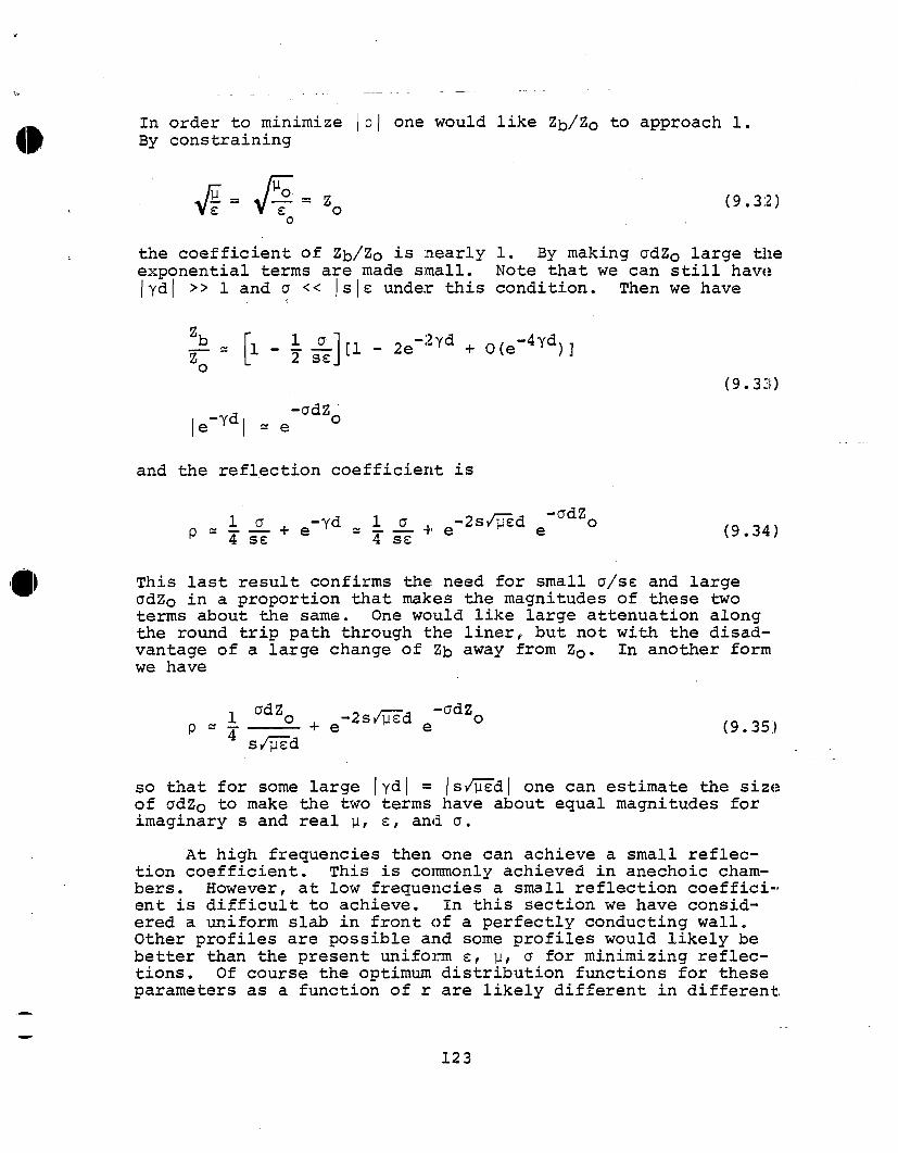
InBy
order to minimize lp\ one would like Zb/Zo to approach 1.constraining
I!=fi=zo (9.3;2)o
the coefficient of Zb/Zo is nearly 1. By making odZo large theexponential terms are made small. Note that we can still haveIydl >>1 and ~ << 1s Ic under this condition. Then we have
[
~= ~ -1020 1T = ‘1 - 2e-2yd + O(e-4yd) ]
(9.33)
and the reflection coefficient is
laP
-d+ e y = ~~+ e-2s@sd e-adzO-—‘4s& 4 SC (9.34)
This last result confirms the need for small ff/scand large6dZo in a proportion that makes the magnitudes of these twoterms about the same. One would like large attenuation alongthe round trip path through the liner, but not with the disad-vantage of a large change of Zb away from 2.. In another formwe have
(9.35)
so that for some large Iydl = Is~d I one can estimate the sizeof adZo to make the two terms have about equal magnitudes forimaginary s and real p, s, and a.
At high frequencies then one can achieve a small reflec-tion coefficient. This is commonly achieved in anechoic cham-bers. However, at low frequencies a small reflection coeffici-ent is difficult to achieve. In this section we have consid-ered a uniform slab in front c]fa perfectly conducting wall.Other profiles are possible and some profiles would likely bebetter than the present uniform c, p, u for minimizing reflec-tions. Of course the optimum distribution functions for theseparameters as a function of r are likely different in different,
123

frequency bands. At high frequencies approximate techniquessuch as a WKBJ solution of Maxwell’s equations are appropriate.
h interesting form of distribution for the constitutiveparameters for r between b and a is
where the identity dyadic is
(9.36)
(9.37)
This form of inhomogeneous anisotropic medium as the dampingand reflection reduction liner still preserves the sphericalsymmetry of-the cavity so that the E and H nmdes still have thesame form as before for r < b and do not couple to each other.For many practical cases one can simply use p = ~. while a + sehas the more general form in equations 9.36 where yr(r,s) andyt(r,s) are chosen so as to be approximately realizable by ar-rays of passive elements.
This general fc?rmof liner given by equations 9.36 needsto be considered in detail from the viewpoints of shifting thenatural frequencies (damping resonances) and reducing reflec-tion magnitudes. Given forms for yr(r,s) and yt(r,s) one needsto consider the approximation of these by arrays of discreteelements. Such arrays do not give the same results as continu-ous distributions and the differences between the two need tobe quantified. Figure 9.2 indicates such a three dimensionalarray. If there is no mutual coupling between elements then Yris directly associated with yr(r,s} for currents in the r di-rection and Yt is directly associated with yt(r,s) for trans-verse currents. Note that displacement current (~) has to beadded to the current through Yr and Yt when designing Yr and Ytto approximate the desired yr and yt.
Note that the use of discrete elements in a damper arrayalso complicates the calculation of the low frequency capaci-tance of the space system with respect to the test chamber.
\ Some effective position of the surface of the liner can be cal-culated for such capacitance purposes.
—
.
h placing a liner inside a cavity the array of elementswill need to allow for the wall curvature which will make theelement spacing vary as one looks at different positions around
124

<
possiblotherginthisregion
Yt
\to spacesystem
Figure 9,2 Three DimensionalArray ofAdmittancesConnectedtoInnermost ElectronTrapping GridF’orReflectionReductionand Damping ofResonances
b
125
,
the liner. The pattern of the element interconnections mayalso need to be changed at various locations to allow for thiscurvature. As the pattern and spacing change the element val-ues Yr and Yt need to be changed so that yr(rfs) and yt(r,s)are correctly approximated. One should account for the shapeof the small volume associated with each Yr and Yt so as tohave the proper relation between the current density averagedover the appropriate cross section and the electric field.Note that the Yr and Yt elements should be small so as to mini-mize collisions of the photons and electrons from the space ve-hicle with these elements. These elements also need sufficientradiation hardness so that their circuit values do not appre-ciably change and noise signals are reasonably small. In somecases these elements might be simple resistive wire.
In a spherical cavity with the space system in the center,waves from the space system reflect back to the space systembecause of the symmetry. One might move the space system offcenter to reduce this reflection problem. Alternatively onemight distort the cavity shape so as to break up any focusingaction back toward the space system. Other cavity shapes suchas finite circular cylinders, rectangular parallelepipeds, andellipsoids are then of interest. The damper design may becomemore complex in some of these geometries. Various such prob-lems need to be considered in detail so as to optimize the testchamber design.
.,
126

i
tor/
Inclusion of Some Other Nuclear and Space EnvironmentalEffects and Instrumentation in the Simulator
There are various requirements on the design of a simula-for the system generated EMP on space systems besides those
associated with the quality of the EMP environment generated.The space system has to be able to function in its normal oper-ational configuration. This implies various features for thesimulator facility depending on each specific space system.For power some-spa”cesyst@rnsdepend on solar energy so the sim-ulator should have light with an appropriate spectrum illumi-nating the solar panels. Normal operational telemetry is alsoneeded so that the space system can function as designed. Thispresents special problems for telemetry antennas near the tankwalls and reflections of the telemetry signals from variousparts of the simulator.
The space system needs to be positioned properly with re-spect to the incident photons. This requires special insulat-ing supports which do not significantly interact with the pho-ton and electron environment. Such dielectric supports must berather sparse... The temperature (and associated heat flow) ap-propriate to the space system configuration needs to beachieved. This is also influenced by the space vacuum condi-tions being simulated. As discussed previously the vacuum con-ditions are important for the electron transport; likewise theearth’s magnetic field is also important.
—
—
There are various other nuclear effects that one might in--elude in a system generated EMP simulator. One might includelate arriving particles (compared to photons) such as neutrons,,electrons, and other charged and neutral particles. Thesewould be provided by separate sources near the photon sourceand would be time tied to the photon source to have the variousparticle fluxes arrive at the proper times relative to theother particles and with the proper waveforms. One might alsoinclude the low energy photons in what is considered the ther-mal range as an appropriate thermal flash with a special gener-’ator.
Instrumentation is important both for simulator performanceand space system response. Electromagnetic fields and relatedelectromagnetic quantities can be monitored near the innermostelectron trapping grid and vacuum tank wall without too muchdifficulty, although transformers with high voltage insulationmay be needed in some cases. For monitoring currents andcharges on the space system one needs telemetry for transmit-ting pulse waveforms using an appropriate modulation scheme.Such a telemetry channel or channels must operate without sig-nificant errors right through the pulse. In other words itmust be radiationtelemetry link on
hard. Furthermore the portions of such athe space system must be small enough and so
127

configured that they do not significantly affect the electro-magnetic response of the space system and in particular thosequantities being measured. Other instrumentation includes mon-itors on the performance of the photon pulser and sensors forthe photon environment produced. Various recording instrumentsand associated recording and control rooms (or other substi-tutes) are also needed.
.
,
1
0 ~128

XI. Overall Simulator Geometry
4BHaving considered many features of”this type of system
generated EMP simulator, some in more detail than others, letus consider what such a simulator might look like from an over-all viewpoint. There are some features which constitute largeportions of such a simulator. First there is the test chamberconsisting of vacuum tank, electron and photon trapping struc-:tures, and damping and reflection reduction structures. Thespace system is placed roughly in the center of this test cham-ber. Second there is a pulseclphoton generator. If a pointsource type of photon generator is used a conical volume isneeded to expand the photons into the test volume. A distrib-uted source photon generator c:anbe placed right next to thetest chamber without a large extension as in tie case of thepoint source. Of course one might construct a point sourcewith conical extension and later convert it to a distributedsource with lower photon energy and perhaps use the conical ex-tension of the vacuum tank to house the distributed source pho-ton generator. One might alsclhave two photon generators, saywith different photon spectra, connected onto the test chamberfrom two different directions. These pulse generators might beused for separate tests. Note that an entry position into thetest chamber is needed to take in and remove the space system.There may also be several electron pulse generators around theboundary of the test chamber for replacing electrons (at alater time) lost from the test volume to the test chamber walls.
Various supporting features, some of it rather large, arealso needed. Coils with power supplies of some type are neededaround the vacuum tank to control the simulation of the earth’smagnetic field in the test chamber. One or more instrumenta-tion rooms are needed for controlling the photon pulserr simu-lated earth’s magnetic field, vacuum in the test chamber, solarpower to the space system, etc. The space system normal oper-ating functions need to be monitored and associated telemetryprovided. This instrumentation room or rooms must also recordvarious transient test data for both the simulator and thespace system. Part of the overall simulator structure might belarge mechanical supports for various items. There is also alarge vacuum pump system to be included. Radiation shieldingis also needed for personnel safety.
suchlatin
There are some optionala simulation facility.,gother nuclear effects .
items that one might include inSome of Wese could be for simu-
These might involve very low en-ergy photons, electrons, neutrons, etc. One might be wary ofintroducing neutrons, however, due to the associated activationproblem.
Figure 11.1 shows a few options for the overall simulatorLayout including the test chamber, pulser, space system entry,and instrumentation (and control) room(s) . As figure 11.1A
129

.
)
photonsource
testchamber
\
groundlevel/////
/ ‘---”h.strumentationand control
room
photonsource
testchamber/
i L--—Jinstrumentationand controlroom
pointphotonsource
A. Photonspropagatinghorizontally
testchamber
P-1spacesystementry
4
ground and controllevel room
//
photonsource
testchamber
1 spacesystementry
4
ground////
\/
level
*< insrutierdationpnoton
and controlsource room
pointphoton distributedphotonsource source
.
B. Photonspropagatingvertically
Figure 11.1 Some OverallC onfigurationsfortheSimulator
130

indicates one might have the direction of photon travel paral-lel to the earth surface. With the simulator laid out likethis, other photon machines can be added which also propagatephotons parallel to the earth toward the space system, but atsome a-ngleother than that of the first photon machine with re-spect to the test chamber and space system. If there is asingle instrumentation and control room it could be placedadjacent to the test chamber at a position which minimizes itsdistance to the main photon pulser”.
As indicated in figure l;L.lBone might have the directionof photon travel upward away :Eromthe earth surface. In such aconfiguration one might place the simulator on the side of ahill so that the pulser, instrumentation and control room, andspace system entry into the test chamber could take place ondifferent levels, all of which would have access to earth sur-face on their own levels. Additional photon pulsers can beadded which propagate photons horizontally. Such pulsers coulcibe placed on a level about the same as the center of the testvolume so as to have ready access from the earth surface on thehillside.
131

XII. Summary
This type of simulator for the system generated EMP isquite different from the common EMP simulators which do nothave nuclear radiation as part of the environment. Its majorcomponents are a pulsed photon source (with appropriate col.Li-mation) and a test chamber which should not significantly back-scatter photons and electrons (in which respect it is partiallya large vacuum tube) and should not significantly alter thespace system response to the system generated EMP (in which re-spect it is partially an anechoic chamber) . There are many de-tailed design calculations needed to optimize the various elec-tromagnetic characteristics of this type of simulator; thisnote considers some of these calculations. There are other de-sign details to be considered in depth which are not linearclassical electromagnetic such as nuclear radiation transport,atomic physics, and nonlinear interaction of electrons (andother charged particles) with the system generated EMP fields.
There is considerable flexibility in the simulator designin the sense that there are alternative designs of pulsers,test chamber shape, and physical layout in connecting the vari-ous major parts together. Such a simulator also can be nmdi-fied after its initial construction in that new radiation puls-ers can be added or changed at later times.
The present note deals with simulation of the system gen-erated EMP on space systems such as satellites. The techniquesdiscussed here can be modified to apply to EMP simulation fornuclear source regions in air. Zn such a case one still needsa pulsed photon machine but the test chamber design and the re-quired air density are somewhat different, but similar consid-erations in the test chamber design are still required.~
.
,%
.
,,
+
\
132

XIII. References
1. Carl E. Baum, Sensor and Simulation Note 151, EM.PSimula-tors for Various Types of Nuclear EMP Environments: An InterimCategorization, July 1972.
,i
2. Capt Carl E. Baum, Interaction Note 76, Electromagnetic“y Pulse Interaction Close to Nuclear Bursts and Associated EMP
Environment Specification, July 1971.
3. W. J. Karzas and R. Latter, Theoretical Note 27, Electro-magnetic Radiation from a Nuclear Explosion in Space, October1961.
4. B. R. Suydam, Theoretical Note 86, Electromagnetic Signalfrom a Bomb Burst in Vacuo, August 1959.
5. S. Glasstone, cd., The Effects of Nuclear Weapons, gov’tprinting office, 1964.
6. Conrad L. Longmire, Theoretical Note 124 (including clas-sified appendix) , External System Generated EMP on Some Typesof Satellite Structure, August 1971. -
7. R. P. Feynman, R. B. Leighton, and M. Sands? The FeynmanLectures on Physics, vol. 1, Addison Wesley, 1966, pp. 41-47.
8. M. Abramowitz and I. A. Stegun, cd., Handbook of Mathemat-ical Functions, ‘AMS 55, National Bureau of S-tandards,1964.
9. R. D. Evans, The Atomic Nucleus, McGraw Hill, 1955, chap-ters 23 through 25.
10. Capt Clovis R. Hale, cd., Theoretical Note 121, A Reviewof Internal EMP Technology, April 1971.
11. Lt Jerry A. Sawyer, Calculation of High-Energy SecondaryElectron Emission, AFSWC-TDR-63-50, August 1963.
12. T. H. Martin, K. R. Prestwich, and D. L. Johnson? Radia-tion Production Note 3, Summary of the Hermes Flash X-Ray Pro-
., gram, October 1969.
13. L. G. Kelly, L. D. Posey, and J. A. Halbeib, A MagneticCompton Spectrometer for High Intensity Pulsed Gamma-Ray En-vironments, IEEE Trans. on Nuclear Science, NS-18 no. 1, Feb-ruary 1971, pp. 131-141.
14. L. D. Posey, private communication, November 1971.
15. Lt Carl E. Baum, Sensor and Simulation Note 15, Radiationand Conductivity Constraints on the Design of a Dipole Electric:Field Sensor, February 1965.
133

.“
16. Lt Carl E. Baum, Sensor and Simulation Note 21, Impedanceand Field Distributions for Parallel Plate Transmission LineSimulators, June 1966.
17. W. R. Smythe, Static and Dynamic Electricity, 3rd cd.,McGraw Hill.,2968, chapter V.
18. Capt Carl E. Baum, Sensor and Simulation Note 38, Param-eters for Some Electrically-Small Electromagnetic Sensors,March 1967. t
19. Capt Carl E. Baum, Sensor and Simulation Note 125, SomeCharacteristics of Electric and Magnetic Dipole Antennas forRadiating Transient Pulses, January 1971.
20. Carl E. Baum, Interaction Note 88, On the Singularity Ex-pansion Method for the Solution of Electromagnetic InteractionProblems, appendix B, December 1971.
21. J. A. Stratton, Electromagnetic Theory, McGraw Hill, 1941,chapter IX.
“*
.
,
134