in defense of parsimony and insight uri shamir
TRANSCRIPT

In Defense of Parsimony and Insight
Uri Shamir
Hydraulics & Waterways Council/WDSA Luncheon & Awards Lecture

In Defense of Parsimony with Insight
Uri Shamir
Hydraulics & Waterways Council/WDSA Luncheon & Awards Lecture

Parsimonyeconomy in the use of means to an end
[also: being careful with money or resources, even stingy]
William of Ockham (c. 1287–1347) an English Franciscan friar and scholastic philosopher
Ockham/Occam's RazorA scientific and philosophical rule requiring that the simplest of
competing theories be preferred to the more complex

The message:Use the simplest model
(conceptual, verbal, mathematical, computational) that meets the
needs of the issue at hand (in terms of the model’s complexity, spatial and temporal detail, parameters, data)

Today’s focus: models for watershed response and for design and management
of water supply systems

Hydrology and Watershed Response

James Clement (Jim) Dooge(1922 – 2010)
1959
Sherman, L.K. (1932) Streamflow from rainfall by the unit-graph method, Engineering News Record 108, 501-505

Dooge, J.C.I. (1997) "Searching for Simplicity in Hydrology“Surveys in Geophysics 18, 511–534
Types of simplification:
(a) simplification of the governing equations;
(b) reduction of the state space, i.e. the number of dependent variables;
(c) reduction of the solution space, i.e. the number of independent variables;
(d) reduction of the parameter space, e.g. by freezing a slowly varying parameter;
(e) simplification of the driving function e.g. Fourier analysis.
James Clement (Jim) Dooge(1922 – 2010)

Dynamic Hydrology McGraw-Hill, 1970Feb. 1928 -

Eagleson, P. S. (1972), “Dynamics of flood frequency”, Water Resources Research, 8(4), 878-898.Derived PDF of runoff and other output parameters, from PDF of rainfall properties “routed” through a simplified watershed model. 20 pages of analytical derivations + graphs of comparison with real data
Analytical derivation
PDF of rainfall properties
Catchment properties
PDF of output


Pete Eagleson had seven(!) papers, 72 pages (!) in a single 1978 issue of Water Resources Research Vol.14, No. 5, pp. 705-776, on “Climate, soil, and vegetation”
1. Introduction to water balance dynamics
2. The distribution of annual precipitation derived from observed storm sequences
3. A simplified model of soil moisture movement in the liquid phase
4. The expected value of annual evapotranspiration
5. A derived distribution of storm surface runoff
6. Dynamics of the annual water balance
7. A derived distribution of annual water yield

Eagleson, P. S. (1978), Water Resources Research Vol.14(5), 741-748
Climate, soil, and vegetation: 5. A derived distribution of storm surface runoffAbstract: The Philip infiltration equation is integrated over the duration of a rainstorm of uniform intensity to give the depth of point surface runoff from such an event on a natural surface in terms of random variables defining the initial soil moisture, the rainfall intensity, and the storm duration. In a zeroth order approximation the initial soil moisture is fixed at its climatic space and time average, whereupon by using exponential probability density functions for storm intensity and duration, the probability density function of point storm rainfall excess is derived. This distribution is used to define the annual average depth of point surface runoff and to derive the flood volume frequency relation, both in terms of a set of physically meaningful climate soil parameters.

Question: what is the response time scale of surface flow in natural
watersheds
Efrat Morin et al., WRR (2002)


Rainfall
Flow at outlet
Rainfall excess
Infiltration
Lateral flow
Hillslope routing
Channel routing
Upstream inflow
Model of a sub-catchment

The responses of the sub-catchments are cascaded in the
watershed topology to generate the total watershed response

The effect of catchment characteristics on the response time scale using distributed model and weather radar information (Morin et al., WRR 2002)
0
5
10
15
20
00 12 00 12 00 12 00Time
Rai
nfal
l int
ensi
ty (m
m/h
)
Catchmenthydrological
response
0
10
20
30
40
00 12 00 12 00 12 00Time
Run
off d
isch
arge
(cm
s)
Ramon98 km2, arid,RTS = 30 min
Evtach48 km2, rural,RTS = 2 hours

0.000
0.010
0.020
0.030
0.040
0.050
0 100 200 300Time scale (min)
PD (1
/min
)
0.000
0.010
0.020
0.030
0.040
0.050
0 100 200 300Time scale (min)
PD (1
/min
)
0.000
0.010
0.020
0.030
0.040
0.050
0 100 200 300Time scale (min)
PD (1
/min
)
0.000
0.010
0.020
0.030
0.040
0.050
0 100 200 300Time scale (min)
PD (1
/min
)
0.000
0.010
0.020
0.030
0.040
0.050
0 100 200 300Time scale (min)
PD (1
/min
)
0.000
0.010
0.020
0.030
0.040
0.050
0 100 200 300Time scale (min)
PD (1
/min
)
0
2
4
6
8
10
12
14
00 12 00 12 00 12 00Time
Rai
nfal
l int
ensi
ty (m
m/h
) 5 minutes
012345678
00 12 00 12 00 12 00Time
Rai
nfal
l int
ensi
ty (m
m/h
) 30 minutes
0
1
2
3
4
5
6
00 12 00 12 00 12 00Time
Rai
nfal
l int
ensi
ty (m
m/h
) 60 minutes
0
1
2
3
4
00 12 00 12 00 12 00Time
Rai
nfal
l int
ensi
ty (m
m/h
) 180 minutes
0
1
2
3
00 12 00 12 00 12 00Time
Rai
nfal
l int
ensi
ty (m
m/h
)
360 minutes
0
5
10
15
20
25
30
00 12 00 12 00 12 00Time
Run
off d
isch
arge
(cm
s) Outlet runoff
0.000
0.010
0.020
0.030
0.040
0.050
0 100 200 300Time scale (min)
PD (1
/min
)
0
1
2
3
4
5
6
00 12 00 12 00 12 00Time
Rai
nfal
l int
ensi
ty (m
m/h
) 90 minutes
0
5
10
15
20
25
30
00 12 00 12 00 12 00Time
Run
off d
isch
arge
(cm
s) Outlet runoff
The Response Time Scale (RTS):The time scale at which the PD of rainfall equal to the PD of runoff
90 min

Can a simple lumped parameter model simulate complex transit time distributions? Benchmarking experiments in a virtual watershed
Daniel Wilusz (JHU), Reed Maxwell (CO School of Mines), Anthony Buda (USDA), William Ball (JHU), Ciaran Harman (JHU)
The student's Award for Best Paper at AGU December 2016
Transit Time Distribution (TTD)


Urban Stormwater ManagementAnalytical solutions for Derived PDFs

Howard, C.D.D. (1976) “Theory of Storage and Treatment-Plant Overflows”, Journal of the Environmental Engineering Division, ASCE, 102(4), 709-722 Chuck HowardUri Shamir & Chuck Howard
Chuck Howard & Uri Shamir
Management of urban stormwater: Analytical-Probabilistic model

Smith, D.I. (1980) “Probability of Overflows for Stormwater Management”, MSc Thesis, University of Toronto Department of Civil Engineering
Howard, C.D.D. (1976) “Theory of Storage and Treatment-Plant Overflows”, Journal of the Environmental Engineering Division, ASCE, 102(4), 709-722 Chuck Howard
Howard, C.D.D., P.E. Flatt, and U. Shamir, "Storm and Combined Sewer Storage-Treatment Theory Compared to Computer Simulation," Grant No. ... III," EPA-600/8284-l09a&b, USEPA, Cincinnati, Ohio, 1989. of Urban Stormwater," EPA-400/3-79-023, USEPA, Washington, D.C., May, 1979.
Uri Shamir & Chuck HowardChuck Howard & Uri Shamir
Barry Adams and Fabian Papa (2000) “Urban Stormwater Management Planning with Analytical Probabilistic Models”, Wiley
Management of urban stormwater: Analytical-Probabilistic model

Given a population of rainstorms, calculate the probabilities of volumes, durations, and inter-storm times -- what is the probability of untreated overflows into the receiving waters
p = overflow, P[p>p0] = Probability of overflow exceeding a stated value p0s = storageΩ = treatment rate capacityb = inter-storm time (exponential, with parameter Ψ)Ψ = 1/(average inter-storm time interval)v = storm volume, (exponential with parameter ζ)ζ = 1/(average storm volume)P[p>p0] = Probability of overflow exceeding a stated value p0t = storm duration (exponential, with parameter λ)λ = 1/(average storm duration)φ = runoff coefficient

SWMM is a distributed, dynamic rainfall-runoff simulation model used for single event or long-term (continuous) simulation of runoff quantity and quality from primarily urban areas. Original SWMM was designed for evaluation of combined sewer overflows (CSOs).
The History and Evolution of the EPA SWMM – Storm Water Management Model (2012)Wayne Huber (OSU) and Lary Roesner (CSU)

A diagnostic assessment of evolutionary algorithms for multi-objective surface water reservoir control Jazmin Zatarain Salazar, Patrick M. Reed, Jonathan D. Herman, Matteo Giuliani, Andrea Castelletti, Advances in Water Resources 92 (2016) 172–185

Water Distribution Systems

Upgrading the Boston Primary Distribution System (1967)
Charles A. Maguire & Assoc., 1968
Work with Chuck Howard, at Charles A. Maguire &Assoc.


The problem: upgrade system performance to meet future demands in the target year
Charles A. Maguire & Assoc., 1967

Approach: a network solver which solves directly for all three types of unknowns - heads, consumptions, link (pipe, pump) properties -
thereby reducing the number of trial-and-error simulations


Main result: a sequence for cleaning and lining pipes, to restore the capacity required to meet future demands
Charles A. Maguire & Assoc., 1967
We imposed two constraints: The pressures should not be reduced while the
sequence of cleaning and lining proceeds Do not change the flow direction in a pipe before it has
been cleaned and lined
Outcome: restoration of system performance with only very few additions, avoiding large capital investment

City of Calgary, Hydraulic Study for Connecting a New Supply, 1970
Underwood McLellan & Assoc., 1970
Determine the economic size of the new pipeline Determine the connection to the city distribution
system Determine the location of storage Engineering analysis: 200 node network model
Cost per network solution ~$ 100. Cost is proportional to (#of nodes)2
Surrogate Model: 19 node reduced network model (“Grey Box”) retaining main and critical demand points and representative conveyance links. Cost per network solution ~$1 Rationale: for the problem at hand do not need a
full network solution, only the pressure and flow “map”
Existing source
From new source

Determine the economic size of the new pipeline Determine the connection to the city distribution
system Determine the location of storage Engineering analysis: 200 node network model
Cost per network solution ~$ 100. Cost is proportional to (#of nodes)2
Surrogate Model: 19 node reduced network model (“Grey Box”) retaining main and critical demand points and representative conveyance links. Cost per network solution ~$1 Rationale: for the problem at hand do not need a
full network solution, only the pressure and flow “map”
Underwood McLellan & Assoc., 1970
City of Calgary, Hydraulic Study for Connecting a New Supply, 1970
From new source
Existing source

Optimal Operation of the Haifa System
Elevations from sea-level to 500 m~100 pressure zones
Shamir & Salomons, JWRPM, 2008

Optimal Operation of the Haifa System
Wadi Risha
KM 4.5
Vulcan
Shamir & Salomons2008
SeaSea
Sea

Optimal Operation of the Haifa System
Shamir & Salomons2008
Detailed Model867 nodes, 987 pipes

Detailed Model867 nodes, 987 pipes
Haifa Water Distribution Model – for optimal operation
Reduced Model77 nodes, 92 pipes
Shamir & Salomons, JWRPM, 2008

Shamir & Salomons, JWRPM, 2008

Pressure at Node 93 - Reduced vs. Full ModelLevel at Tank 12 - Reduced vs. Full Model
Shamir & Salomons, JWRPM, 2008

BATtle of the Attack Detection ALgorithms (BATADAL)http://batadal.net/schedule.html
Annual Water Distribution Systems Analysis SymposiumSacramento, California, U.S.A.May 21-25, 2017
Organizing Committee: Ricardo Taormina, Stefano Galelli, Nils Ole Tippenhauer
Graphical representation of C-Town water distribution system

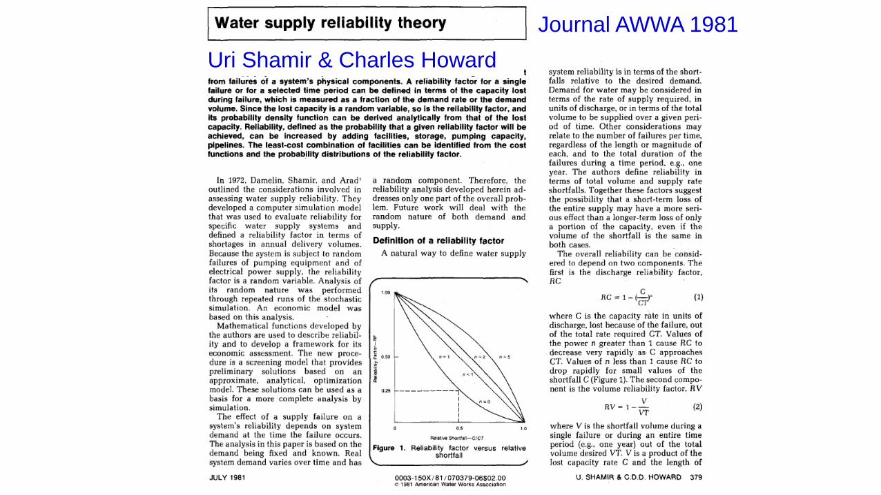
Reliability of Water Supply Systems
University of Calgary - 8 May 2007
Journal AWWA 1981Uri Shamir & Charles Howard

Effect of Storage on Reliability
Minimum Cost curves vs Reliability
Standby Pumping Capacity vs. Storage and for given Reliability
Rel
Reliability
Reliability
Min Cost
SBP
Storage
Shamir & Howard, JAWWA 1981
Tradeoffs between: pumping capacity, storage, cost & reliability
Min Cost path
Storage

Water Supply ReliabilityRegional Municipality of Ottawa-Carlton – 1995
Charles Howard and Associates Ltd.

Municipality of Ottawa-Carlton, 1995

Demand Elasticity
Shortage as fraction of daily demand
Shortage
Cost
(K$/day)
Larger (negative) Elasticity Lower Loss
Municipality of Ottawa-Carlton, 1995

Supply/Demand (%)
Annual
Cost
$M
Shortage
Capital
Total Cost
Reliability
Reliability
Municipality of Ottawa-Carlton, 1995

An analytic approach to scheduling pipeline replacementUri Shamir and Charles D.D. HowardJournal of the American Water Works Association, Vol. 71, No. 5, pp. 248-258, May 1979
Developed for Calgary, to address the problem of ~1,000 pipe breaks per year, with a total repair cost of ~1.5 M$ per year
Data: statistical projection of breaks/year based on historical data + cost of repairing a break and of replacing the pipe + interest rate

Models for Operational Management of the Israeli
National System

Western Galilee Aquifer
Carmel Aquifer
Coastal Aquifer
N. EastMountain
AquiferEastWest
Lake
Tel Aviv
Jerusalem
Haifa
Negev Aq.
Arava Aq.
Kinneret Watershed
Main WaterSystems
Av. replenishment (mcm/year)Med. Sea to Jordan R. ~ 1,700 Considered for Israel ~ 1,200
Integrated National and Regional Water Systems
~25% Beyond Israel’s border

Natural Replenishment (mcm/year)
1973-1992Av = 1,848SD = 684
1993-2009Av = 1,643SD = 465
1973-2009Av = 1,748SD = 584
Cum. Deficit~1,770 mcm
Cum. Deficit 1,526+ mcm
1991/1992 - 3,839 mcm (Pinatubo?)
All Sources from Mediterranean Sea to Jordan River (exc. Gaza)
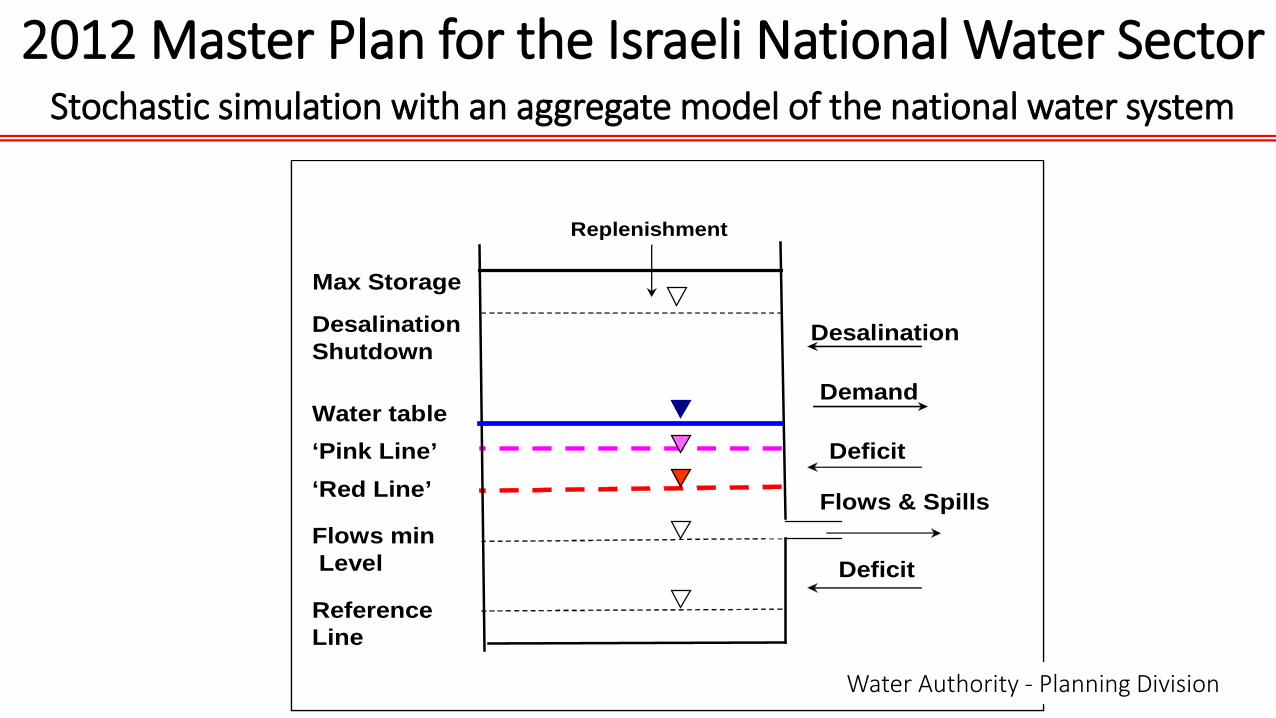
Max Storage
Desalination Shutdown
Water table‘Pink Line’‘Red Line’
Flows min Level
Reference Line
Replenishment
Desalination
Demand
Deficit
Deficit
Flows & Spills
Max Storage
Desalination Shutdown
Water table‘Pink Line’‘Red Line’
Flows min Level
Reference Line
Replenishment
Desalination
Demand
Deficit
Deficit
Flows & Spills
2012 Master Plan for the Israeli National Water SectorStochastic simulation with an aggregate model of the national water system
Water Authority - Planning Division

התפלה נדרשת כתלות במדיניות אמינות אספקה*
0100200300400500600700800900
1,0001,1001,2001,3001,4001,5001,6001,700
2015 2020 2025 2030 2035 2040 2045 2050שנה
"קמ
מלה,
פלת
ה
75% 90%95% 100%מחסור מקסימאלי 250 מלמ"ש תוכנית מאושרתתוכנית מומלצת
נבחנה על בסיס תרחישים שהוגדרו *
Development of Desalination Capacity for the Required Reliability
Desa
linat
ion
Capa
city
, mcm
/yea
r
Water Authority - Planning Division
Max shortfall 250 mcm/yr Approved planRecommended Plan

60
Ashkelon: 100 mcm/y (2006)120
Palmachim: 45 mcm/y (2007) 90
Hadera: 100 mcm/y (2009) 127
Sorek: 150 mcm/y (2016)
PlannedWith Ashdod (full) 587 mcm~50% of the average natural fresh water
Ashdod: 100 mcm (?)Some difficulties encountered
+ Brackish GW desalination 55 mcm/y

National Model with Natural and Desalinated Waters
Objective: minimum total annual cost - of production, transport and delivery.
The results are monthly and annual water productions, flows and salinities, displayed directly on the schematic and in tables.
Can page through the annual and monthly results - shown on the schematic.

National Model with Natural and Desalinated Waters
A model run takes several seconds and the results are available in real time - at working and policy sessions –so that different conditions, data, policy parameters, and design changes can be tested and evaluated interactively.
The deterministic model can operate as a kernel for stochastic optimization.

Jordan-Israel Water Agreement
A component of the Jordan-Israel 1994 Peace Treaty

Pragmatic & parsimonious Where (location: Yarmouk, Jordan River, GW in the Arava)
When (season: winter, summer)
Allocations (between the Parties from each of several sources)
The rule: A gets a low firm quantity, B gets all the rest
Quality (of the water transferred by A to B)
Cost (price B pays to A)
Israel-Palestinian Water Agreement 1995 (Oslo II, Interim) – similar approach re allocation of sources

Messages

Use the simplest model (conceptual, verbal, mathematical, computational) that meets the
needs of the issue at hand (in terms of the model’s complexity, spatial and temporal detail, parameters, data)

Do not be swayed merely by the advent of fancier, more complex and detailed models, nor by the
access to ever greater computing power

Spend more effort and time on insight than on computation

I have great expectations for Data Mining, Big Data, Evolutionary Algorithms
They have their role in gaining insight to data, to system performance, to underlying principles
But for creative engineering and management they may mask the need for in-depth thinking and are not ideal for communication with and among stakeholders and decision makers

And bear in mind that:The model is a platform for
disciplined discourse, in support of decision making
Uri Shamir, ~1995

In Support of Parsimony and Insight
Uri Shamir
Hydraulics & Waterways Council/WDSA Luncheon & Awards Lecture