in copyright - non-commercial use permitted rights ...28684/... · the stability of dark matter...
TRANSCRIPT

Research Collection
Master Thesis
The stability of dark matter cusps
Author(s): Zemp, Marcel
Publication Date: 2003
Permanent Link: https://doi.org/10.3929/ethz-a-005187379
Rights / License: In Copyright - Non-Commercial Use Permitted
This page was generated automatically upon download from the ETH Zurich Research Collection. For moreinformation please consult the Terms of use.
ETH Library

The Stability of Dark Matter Cusps
Marcel Zemp
ETH Zurich
November 2002 - February 2003
Diploma Thesis
carried out at the Institute of Theoretical Physics of the University of Zurichunder supervision of Prof. Dr. Ben Moore.
Version 1.2

ii

Contents
I Introduction and Fundamentals 1
1 Dark Matter 31.1 Cosmological Framework . . . . . . . . . . . . . . . . . . . . . . . . . . . . . . 3
1.1.1 Friedmann-Robertson-Walker Universe . . . . . . . . . . . . . . . . . . 31.1.2 Hubble Law . . . . . . . . . . . . . . . . . . . . . . . . . . . . . . . . . 41.1.3 Concordance Model of Cosmology . . . . . . . . . . . . . . . . . . . . 4
1.2 Mass Estimation Tools . . . . . . . . . . . . . . . . . . . . . . . . . . . . . . . 61.2.1 Mass-to-Light Ratio . . . . . . . . . . . . . . . . . . . . . . . . . . . . 61.2.2 Virial Theorem . . . . . . . . . . . . . . . . . . . . . . . . . . . . . . . 6
1.3 Evidence for Dark Matter . . . . . . . . . . . . . . . . . . . . . . . . . . . . . 81.3.1 First Speculation about Dark Matter . . . . . . . . . . . . . . . . . . . 81.3.2 Dark Matter on different Scales . . . . . . . . . . . . . . . . . . . . . . 8
1.4 Dark Matter Candidates . . . . . . . . . . . . . . . . . . . . . . . . . . . . . . 111.4.1 Estimations of the different Mass Components . . . . . . . . . . . . . 111.4.2 Classification of Dark Matter . . . . . . . . . . . . . . . . . . . . . . . 111.4.3 Baryonic Dark Matter . . . . . . . . . . . . . . . . . . . . . . . . . . . 111.4.4 Non-baryonic Dark Matter . . . . . . . . . . . . . . . . . . . . . . . . 12
2 Modelling Dark Matter Halos 152.1 Statistical Mechanics and Potential Theory . . . . . . . . . . . . . . . . . . . 15
2.1.1 Phase Space and Distribution Function . . . . . . . . . . . . . . . . . 152.1.2 Collisionless Boltzmann Equation . . . . . . . . . . . . . . . . . . . . . 162.1.3 Poisson Equation . . . . . . . . . . . . . . . . . . . . . . . . . . . . . . 162.1.4 Steady-state Solutions . . . . . . . . . . . . . . . . . . . . . . . . . . . 16
2.2 Cuspy Halos . . . . . . . . . . . . . . . . . . . . . . . . . . . . . . . . . . . . . 172.2.1 Density Profile for r ≤ rvir . . . . . . . . . . . . . . . . . . . . . . . . 172.2.2 Scale Radius and virial Radius . . . . . . . . . . . . . . . . . . . . . . 182.2.3 Characteristic Density . . . . . . . . . . . . . . . . . . . . . . . . . . . 182.2.4 Density Profile for r ≥ rvir . . . . . . . . . . . . . . . . . . . . . . . . 192.2.5 Categories of Density Profiles . . . . . . . . . . . . . . . . . . . . . . . 20
2.3 Calculating the Distribution Function . . . . . . . . . . . . . . . . . . . . . . 202.3.1 Spherical Systems and Anisotropy Parameter . . . . . . . . . . . . . . 222.3.2 General Solution for an isotropic Velocity Dispersion . . . . . . . . . . 222.3.3 Derivatives of the Density Profile . . . . . . . . . . . . . . . . . . . . . 23
2.4 Halos with constant Density Core . . . . . . . . . . . . . . . . . . . . . . . . . 252.4.1 Density Profile . . . . . . . . . . . . . . . . . . . . . . . . . . . . . . . 25
iii

iv CONTENTS
2.4.2 Distribution Function . . . . . . . . . . . . . . . . . . . . . . . . . . . 262.4.3 Characteristic Density . . . . . . . . . . . . . . . . . . . . . . . . . . . 27
II Simulations 29
3 Shell Model Halos 313.1 Initial Conditions . . . . . . . . . . . . . . . . . . . . . . . . . . . . . . . . . . 31
3.1.1 Dark Matter Halo . . . . . . . . . . . . . . . . . . . . . . . . . . . . . 313.2 Simulation and Results . . . . . . . . . . . . . . . . . . . . . . . . . . . . . . . 31
3.2.1 Stability . . . . . . . . . . . . . . . . . . . . . . . . . . . . . . . . . . . 32
4 Sinking Black Hole 334.1 Initial Conditions . . . . . . . . . . . . . . . . . . . . . . . . . . . . . . . . . . 33
4.1.1 Dark Matter Halo . . . . . . . . . . . . . . . . . . . . . . . . . . . . . 334.1.2 Black Hole . . . . . . . . . . . . . . . . . . . . . . . . . . . . . . . . . 33
4.2 Simulation and Results . . . . . . . . . . . . . . . . . . . . . . . . . . . . . . . 334.2.1 Dynamical Friction Time . . . . . . . . . . . . . . . . . . . . . . . . . 344.2.2 Evolution of Density Profiles and Anisotropy Parameters . . . . . . . 344.2.3 Stability . . . . . . . . . . . . . . . . . . . . . . . . . . . . . . . . . . . 35
5 Merger Sequence 375.1 Initial Conditions . . . . . . . . . . . . . . . . . . . . . . . . . . . . . . . . . . 37
5.1.1 Dark Matter Halo . . . . . . . . . . . . . . . . . . . . . . . . . . . . . 375.1.2 Black Hole . . . . . . . . . . . . . . . . . . . . . . . . . . . . . . . . . 385.1.3 Merger Set-up . . . . . . . . . . . . . . . . . . . . . . . . . . . . . . . 38
5.2 Simulation and Results . . . . . . . . . . . . . . . . . . . . . . . . . . . . . . . 395.2.1 Black Hole Separation . . . . . . . . . . . . . . . . . . . . . . . . . . . 395.2.2 Halo Merger Time . . . . . . . . . . . . . . . . . . . . . . . . . . . . . 395.2.3 Black Hole Merger Time . . . . . . . . . . . . . . . . . . . . . . . . . . 405.2.4 Evolution of Density Profiles . . . . . . . . . . . . . . . . . . . . . . . 40
6 Halos with constant Density Core 436.1 Initial Conditions . . . . . . . . . . . . . . . . . . . . . . . . . . . . . . . . . . 43
6.1.1 Dark Matter Halo . . . . . . . . . . . . . . . . . . . . . . . . . . . . . 436.1.2 Merger Set-up . . . . . . . . . . . . . . . . . . . . . . . . . . . . . . . 43
6.2 Simulation and Results . . . . . . . . . . . . . . . . . . . . . . . . . . . . . . . 436.2.1 Stability . . . . . . . . . . . . . . . . . . . . . . . . . . . . . . . . . . . 436.2.2 Mergers . . . . . . . . . . . . . . . . . . . . . . . . . . . . . . . . . . . 44
III Appendix 47
A Some useful astrophysical Constants 49

CONTENTS v
B Where is the maximum circular Velocity reached? 51B.1 Criteria for maximum circular Velocity . . . . . . . . . . . . . . . . . . . . . . 51B.2 Moore Profile . . . . . . . . . . . . . . . . . . . . . . . . . . . . . . . . . . . . 52B.3 NFW Profile . . . . . . . . . . . . . . . . . . . . . . . . . . . . . . . . . . . . 52B.4 Concentration Relation . . . . . . . . . . . . . . . . . . . . . . . . . . . . . . 53B.5 Merger Sequence - Exact Results . . . . . . . . . . . . . . . . . . . . . . . . . 54
C Software Tools 55C.1 Available Software . . . . . . . . . . . . . . . . . . . . . . . . . . . . . . . . . 55
C.1.1 MAKEHALO . . . . . . . . . . . . . . . . . . . . . . . . . . . . . . . . 55C.1.2 PKDGRAV . . . . . . . . . . . . . . . . . . . . . . . . . . . . . . . . . 55C.1.3 TIPSY . . . . . . . . . . . . . . . . . . . . . . . . . . . . . . . . . . . . 55C.1.4 Super Mongo . . . . . . . . . . . . . . . . . . . . . . . . . . . . . . . . 55
C.2 Self-written Programs . . . . . . . . . . . . . . . . . . . . . . . . . . . . . . . 56C.2.1 Composeascii . . . . . . . . . . . . . . . . . . . . . . . . . . . . . . . . 56C.2.2 Readstarxv . . . . . . . . . . . . . . . . . . . . . . . . . . . . . . . . . 56
D Detailed Halo Specifications 57D.1 HALO A . . . . . . . . . . . . . . . . . . . . . . . . . . . . . . . . . . . . . . 57D.2 HALO B . . . . . . . . . . . . . . . . . . . . . . . . . . . . . . . . . . . . . . . 58D.3 HALO C . . . . . . . . . . . . . . . . . . . . . . . . . . . . . . . . . . . . . . . 58D.4 HALO D . . . . . . . . . . . . . . . . . . . . . . . . . . . . . . . . . . . . . . 59D.5 HALO E . . . . . . . . . . . . . . . . . . . . . . . . . . . . . . . . . . . . . . . 59D.6 HALO F . . . . . . . . . . . . . . . . . . . . . . . . . . . . . . . . . . . . . . . 60D.7 HALO G . . . . . . . . . . . . . . . . . . . . . . . . . . . . . . . . . . . . . . 60

vi CONTENTS
List of Figures
1.1 Cosmic triangle . . . . . . . . . . . . . . . . . . . . . . . . . . . . . . . . . . . 51.2 Circular velocity curve for NGC 6503 . . . . . . . . . . . . . . . . . . . . . . . 10
2.1 Moore and NFW density profiles . . . . . . . . . . . . . . . . . . . . . . . . . 21
3.1 Density profiles for shell model halo . . . . . . . . . . . . . . . . . . . . . . . 32
4.1 Density profiles for sinking black hole simulation . . . . . . . . . . . . . . . . 344.2 Anisotropy parameter for sinking black hole simulation . . . . . . . . . . . . . 354.3 Density profile and anisotropy parameter for reference simulation . . . . . . . 36
5.1 Circular velocity curves for merger sequence . . . . . . . . . . . . . . . . . . . 385.2 Black hole separations . . . . . . . . . . . . . . . . . . . . . . . . . . . . . . . 415.3 Dark matter density profiles for merger sequence . . . . . . . . . . . . . . . . 42
6.1 Density profiles for a single cored halo . . . . . . . . . . . . . . . . . . . . . . 446.2 Density profiles for cored halos after merger . . . . . . . . . . . . . . . . . . . 45
B.1 Circular velocity curve for a Moore and a NFW profile . . . . . . . . . . . . . 54
vii

viii LIST OF FIGURES

Preface
The decision to do my diploma thesis in the area of numerical research in astrophysics cameafter I took the course in Astronomy by Prof. Dr. Ben Moore in summer term 2002. Iwas fascinated by the movies and pictures from the simulations that were shown during thelectures. Especially one movie showing the formation of structure in a large cube of theuniverse was very impressing. This revealed to me the enormous facilities that lie in this forme to that date totally unknown field of science and I decided to do my diploma thesis innumerical simulations.
In this thesis, I investigated the stability of dark matter halos e.g. What happens to thedensity profile if a black hole is sinking to the centre of the halo? How is a halo mergeraffected if the initial halos contain a central supermassive black hole? Does violent relaxationestablish a new cusp in a merger with initially cored halos? These were the main questions Itried to answer in this thesis.
This diploma thesis is organised the following way. In part I, an overview chapter on darkmatter is presented followed by the basic concepts and underlying theory in chapter 2. Inpart II, I present the results of the performed simulations and part III is the appendix.
At this place, I would also like to take the opportunity to thank Prof. Dr. Ben Moore forhis ideas and inspiration for this diploma thesis and always having time for me to discussthe results although his busy schedule has only a few spare places. I owe also a lot toStelios Kazantzidis. He introduced me to his programs and found always time to answer myquestions. In addition, I would like to thank to Jurg Diemand who executed my simulations atthe SCSC in Manno and the new supercomputer (zBox) of the group of Ben Moore. Further,I thank all the people at the Institute of Theoretical Physics of University of Zurich for theirhospitality and helpfullness, especially all the people in the group of Ben Moore.
After this diploma thesis, I’m convinced that computer simulations combined with inputparameters from observations are one of the most promissing tools to answer the questionsof today’s cosmology and astrophysics.
Marcel Zemp1
February 2003
1E-mail: [email protected]
ix

x LIST OF FIGURES

Part I
Introduction and Fundamentals
1

Chapter 1
Dark Matter
The aim of this chapter is to give an overview of the dark matter topic. It is not intended togive a complete survey. Thus, not too much details are presented and it is meant to give theidea of the basic concepts. The only exception is the virial theorem which is completely derivedhere as an example for the beauty of classical mechanics and its application to astrophysics.
1.1 Cosmological Framework
In order to see how the dark matter problem arises, one needs to understand the underlyingframework of the modern standard model of cosmology and its basic concepts.
1.1.1 Friedmann-Robertson-Walker Universe
The basic theory for the Friedmann-Robertson-Walker Universe is the theory of general rel-ativity. Under the assumption of isotropy and homogeneity the metric takes the form1
ds2 = dt2 −R2(t)[
dr2
1− kr2+ r2
(dϑ2 + sin2(ϑ)dϕ2
)](1.1)
and is called the Robertson-Walker metric. The radial comoving coordinate is denoted by r,ϕ and ϑ are the angular coordinates, k is the curvature parameter and R(t) is the expansionfactor.
Einstein’s famous field equation Gµν = 8πGTµν + Λgµν in its general form with the cosmo-logical constant Λ reduces with this metric to the Friedmann equation
(R
R
)2
=8πG
3ρ +
Λ3− k
R2. (1.2)
The Hubble parameter at any epoch is defined by
H ≡ R
R= 100× h km s−1 Mpc−1 (1.3)
where h ≈ 0.7 at this epoch. The definition of the critical density at any time is given by
1As usual in cosmology and general relativity, we set the speed of light c ≡ 1.
3
4 CHAPTER 1. DARK MATTER
ρc ≡ 3H2
8πG= 1.879× 10⁻²⁶ h2 kg m−3 . (1.4)
Thus, we obtain form the Friedmann equation 1.2 with Ωi ≡ ρi
ρcfor any epoch
1 =∑
i
Ωi . (1.5)
This equation determines the contribution of every possible energy component in the universe,e.g. non-relativistic matter, relativistic matter, dark energy (ΩΛ ≡ Λ
3H2 ) and the curvaturepart (ΩK ≡ − k
R2H2 ).
1.1.2 Hubble Law
Hubble investigated the spectral features of galaxies and showed in 1929 that they displayed ashift to longer wavelengths that is proportional to the distances to the galaxies. The redshiftz is defined as
z ≡ λobserved − λemitted
λemitted. (1.6)
In the limit of small redshifts, z ¿ 1, it follows from the relativistic Doppler effect that z ≈ vc .
So we can write the famous Hubble law2 as
v = Hd , (1.7)
where H, the Hubble parameter introduced in equation 1.3, is the proportionality parame-ter.3 This general tendency for all celestial objects to drift away from each other due to theexpansion of the Universe is called the Hubble flow.
1.1.3 Concordance Model of Cosmology
From many observations e.g CMB spectra (Cosmic Microwave Background) or supernovaeIa follow constraints to the different possible parameters in cosmology. The parameters areinternally consistent and the result is the concordance model of cosmology with the followingimportant parameters at this epoch4
Ω0M ≈ 0.3 Ω0
Λ ≈ 0.7 Ω0R ≈ 10−5 Ω0
K ≈ 0 h0 ≈ 0.7 .
The subscript M means matter, Λ denotes dark energy (Λ-Term), R stands for radiation, Kis for curvature and h is the Hubble parameter as defined in 1.3.
We see that at this epoch the universe is not any more radiation dominated as it was before theradiation decoupled form the matter and we can neglect the influence of radiation nowadays.Throughout this paper we will work with these values of the parameters. These values of thecosmological parameters are consistent with the latest results found by WMAP [1].
2From d ≡ R(t)r and v ≡ d = R(t)r, the Hubble law follows directly.3Therefore, one chooses to quote lengths in astrophysics l ∝ h−1, e.g. 1.23 h−1Mpc. From equation 1.4
follows that masses are also quoted with a proportionality to h−1, e.g. 1× 10¹² h−1M¯.4Values of the cosmological parameters at this epoch are denoted by a super- or subscript 0.

1.1. COSMOLOGICAL FRAMEWORK 5
Figure 1.1: The cosmic triangle represents the three parameters ΩM , ΩK and ΩΛ. SCDMdenotes the Standard Cold Dark Matter model with ΩM ≈ 1.0, ΩΛ ≈ 0 and ΩK ≈ 0, OCDMis the Open Cold Dark Matter model with ΩM ≈ 0.3, ΩΛ ≈ 0 and ΩK ≈ 0.7. The remainingmodel with a non-zero cosmological constant Λ and ΩM ≈ 0.3, ΩΛ ≈ 0.7 and ΩK ≈ 0 is calledthe ΛCDM model. Each point in the diagram satisfies the Friedmann condition 1.5. Thefavoured model from the observations is the ΛCDM-model (our concordance model).

6 CHAPTER 1. DARK MATTER
1.2 Mass Estimation Tools
The mass-to-light ratio and virial theorem are two tools to estimate the mass of objects in theuniverse as e.g. galaxies and clusters of galaxies. The virial theorem is a beautiful applicationof classical mechanics.
1.2.1 Mass-to-Light Ratio
All light emitting objects can be characterised by the emitted energy per unit mass. Thisparameter is called the mass-to-light ratio M/L between the dynamical mass M and theluminosity L. For cosmological purposes, the mass-to-light ratio is expressed in units of solarmass per solar luminosity, M¯/L¯.
There can be shown that for stars in the main sequence of the Hertzsprung-Russell diagramthe luminosity L and the mass M are related by (L/L¯) ∝ (M/M¯)n where n ≈ 3.5 − 4.Thus, a 10 M¯ star has M/L ≈ 10−3M¯/L¯ whereas a 0.1 M¯ star has M/L ≈ 103M¯/L¯.
1.2.2 Virial Theorem
When an astrophysical system has formed and reaches an equilibrium state (e.g. galaxies)then this astrophysical system is called virialised and we can apply the virial theorem.
For a system of N mutually gravitating particles with masses mα and positions xα, thecomponents of the moment of inertia tensor I are defined by
Ijk ≡N∑
α=1
mαxαj xα
k . (1.8)
From the first time derivative
dIjk
dt=
N∑
α=1
mα
(xα
j xαk + xα
j xαk
), (1.9)
follows immediately the second time derivative
d2Ijk
dt2=
N∑
α=1
mα
(xα
j xαk + 2xα
j xαk + xα
j xαk
). (1.10)
The acceleration of the particle α caused by the gravitational force of the other particles isgiven by
xαl =
N∑
β=1β 6=α
Gmβxβ
l − xαl
|xα − xβ|3 . (1.11)
After substituting this result into equation 1.10 we obtain
d2Ijk
dt2= 2
N∑
α=1
mαxαj xα
k +N∑
α,β=1β 6=α
Gmαmβ
(xβj − xα
j )xαk + xα
j (xβk − xα
k )|xα − xβ|3 . (1.12)

1.2. MASS ESTIMATION TOOLS 7
We define the components of the kinetic energy tensor K by
Kjk ≡ 12
N∑
α=1
mαxαj xα
k . (1.13)
In an analogous way, we define the components of the potential energy tensor W5
Wjk ≡N∑
α=1
mαxαj xα
k (1.14)
= GN∑
α,β=1β 6=α
mαmβ
xαj (xβ
k − xαk )
|xα − xβ|3 (1.15)
= −12
G
N∑
α,β=1β 6=α
mαmβ
(xαj − xβ
j )(xαk − xβ
k)|xα − xβ|3 , (1.16)
where the last line is obtained by symmetrisation and it is explicitly obvious that the potentialenergy tensor W is symmetric, Wjk = Wkj .
By going back to equation 1.12 we identify the first term on the right side by 4Kjk and thesecond term by Wkj + Wjk = 2Wjk and we finally obtain
12
d2Ijk
dt2= 2Kjk + Wjk . (1.17)
Equation 1.17 is called the tensor virial theorem.
If we take the trace of each tensor i.e. I ≡ tr(I) and use our condition that the astrophysicalsystem is virialised so that d2I
dt2= 0, then equation 1.17 becomes the scalar virial theorem
2K + W = 0 (1.18)
where
K ≡ tr(K) =12
N∑
α=1
mα
3∑
i=1
(xαi )2 =
12
N∑
α=1
mαv2α (1.19)
W ≡ tr(W) = −12
GN∑
α,β=1β 6=α
mαmβ
3∑
i=1
(xαi − xβ
i )2
|xα − xβ|3 = −12
GN∑
α,β=1β 6=α
mαmβ
|xα − xβ| (1.20)
are the kinetic energy and the potential energy respectively. If we denote the total energy byE = K + W , then an alternative expression of the scalar virial theorem is
E = K + W = −K =12W (1.21)
5Also known as the Chandrasekhar potential energy tensor.
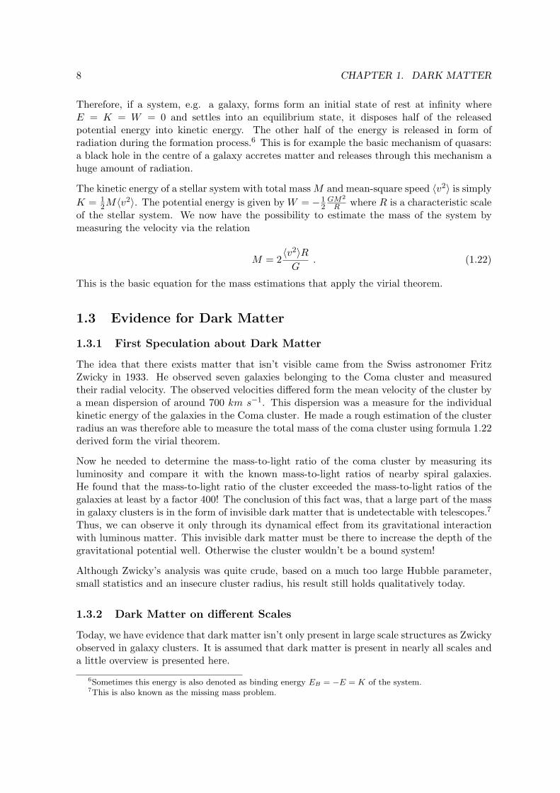
8 CHAPTER 1. DARK MATTER
Therefore, if a system, e.g. a galaxy, forms form an initial state of rest at infinity whereE = K = W = 0 and settles into an equilibrium state, it disposes half of the releasedpotential energy into kinetic energy. The other half of the energy is released in form ofradiation during the formation process.6 This is for example the basic mechanism of quasars:a black hole in the centre of a galaxy accretes matter and releases through this mechanism ahuge amount of radiation.
The kinetic energy of a stellar system with total mass M and mean-square speed 〈v2〉 is simplyK = 1
2M〈v2〉. The potential energy is given by W = −12
GM2
R where R is a characteristic scaleof the stellar system. We now have the possibility to estimate the mass of the system bymeasuring the velocity via the relation
M = 2〈v2〉R
G. (1.22)
This is the basic equation for the mass estimations that apply the virial theorem.
1.3 Evidence for Dark Matter
1.3.1 First Speculation about Dark Matter
The idea that there exists matter that isn’t visible came from the Swiss astronomer FritzZwicky in 1933. He observed seven galaxies belonging to the Coma cluster and measuredtheir radial velocity. The observed velocities differed form the mean velocity of the cluster bya mean dispersion of around 700 km s−1. This dispersion was a measure for the individualkinetic energy of the galaxies in the Coma cluster. He made a rough estimation of the clusterradius an was therefore able to measure the total mass of the coma cluster using formula 1.22derived form the virial theorem.
Now he needed to determine the mass-to-light ratio of the coma cluster by measuring itsluminosity and compare it with the known mass-to-light ratios of nearby spiral galaxies.He found that the mass-to-light ratio of the cluster exceeded the mass-to-light ratios of thegalaxies at least by a factor 400! The conclusion of this fact was, that a large part of the massin galaxy clusters is in the form of invisible dark matter that is undetectable with telescopes.7
Thus, we can observe it only through its dynamical effect from its gravitational interactionwith luminous matter. This invisible dark matter must be there to increase the depth of thegravitational potential well. Otherwise the cluster wouldn’t be a bound system!
Although Zwicky’s analysis was quite crude, based on a much too large Hubble parameter,small statistics and an insecure cluster radius, his result still holds qualitatively today.
1.3.2 Dark Matter on different Scales
Today, we have evidence that dark matter isn’t only present in large scale structures as Zwickyobserved in galaxy clusters. It is assumed that dark matter is present in nearly all scales anda little overview is presented here.
6Sometimes this energy is also denoted as binding energy EB = −E = K of the system.7This is also known as the missing mass problem.

1.3. EVIDENCE FOR DARK MATTER 9
Dwarf Spheroidals and globular Clusters
Small stellar systems as dwarf spheroidals orbiting the Milky Way provide through theirdynamics evidence for dark matter. Dwarf spheroidals are small galaxies with about 106
stars and have a similar luminosity to globular clusters. There exist several of them thatorbit our Galaxy and by measuring the velocities of the individual stars one finds that theyare moving at v ≈ 10 km s−1. From the observed mass of stars, these velocities are an order ofmagnitude larger than expected. To bound these fast stars to the dwarf spheroidal there hasto be an additional mass that is invisible. Thus, dwarf spheroidals are completely dominatedby dark matter and are the smallest systems within which dark matter is observed.
In contrast, globular clusters are 10-100 times smaller but have a similar amount of starsas dwarf spheroidals. A stream of stars escaping these stellar systems is detected. Thegravitational field of the Milky Way removes the least bound stars from the globular cluster.It therefore appears that globular clusters don’t contain any dark matter. These tails ofescaping stars are called tidal streams.
Galaxies
A very crucial evidence for dark matter comes from rotation curves of spiral galaxies. Mostof the galaxies in our universe are spiral galaxies, like our own host galaxy the Milky Way.The stars and gas in these spiral galaxies move on circular orbits within a thin disk. It isobserved, that after a steep rise in the central region, the velocities remain constant. Fromthe centripetal force F = mv2
r and Newton’s law of gravity F = GM(r)mr2 follows the relation
GM(r)r2 = v2
r and therefrom directly the definition of the circular velocity at radius r for aspherical system
vc(r) ≡√
GM(r)r
, (1.23)
where M(r) denotes the accumulated mass function. This implies that in the inner regionwhere the velocity rises linearly the mass is proportional to M(r) ∝ r3 and therefore hasclose to constant density. In regions where the circular velocity is constant, the accumulatedmass is proportional to the radius r, M(r) ∝ r and the mass density drops like ρ(r) ∝ r−2.8
The transition region from inner, constant density region, to the outer, flat rotation curveregion occurs at the scale radius rs. Once r becomes greater than the extent of the mass, oneexpects the velocities to drop v ∝
√r−1, thus called Keplerian region.
By using the 21 cm emission lines of clouds of neutral hydrogen9 the velocities v can be mea-sured at much larger radii. These observations showed that the circular velocities still remainconstant and that there is no sign of the expected Keplerian fall-off. A simple explanation ofthese flat rotation curves is, that galaxies are surrounded by massive dark matter halos thatextend to larger radii than the optical disks.
This idea of an additional mass component to the visible component is also supported bystudying the velocities of very fast stars that are bound to our galaxy, the Milky Way. To
8Models with such a density profile are called isothermal.9Due to nucleus-electron spin interaction, the level 1S1/2 of hydrogen is splitted into a doublet and the
degeneracy is broken. The energy difference between these two levels corresponds to a photon with wavelengthλ ≈ 21 cm.
10 CHAPTER 1. DARK MATTER
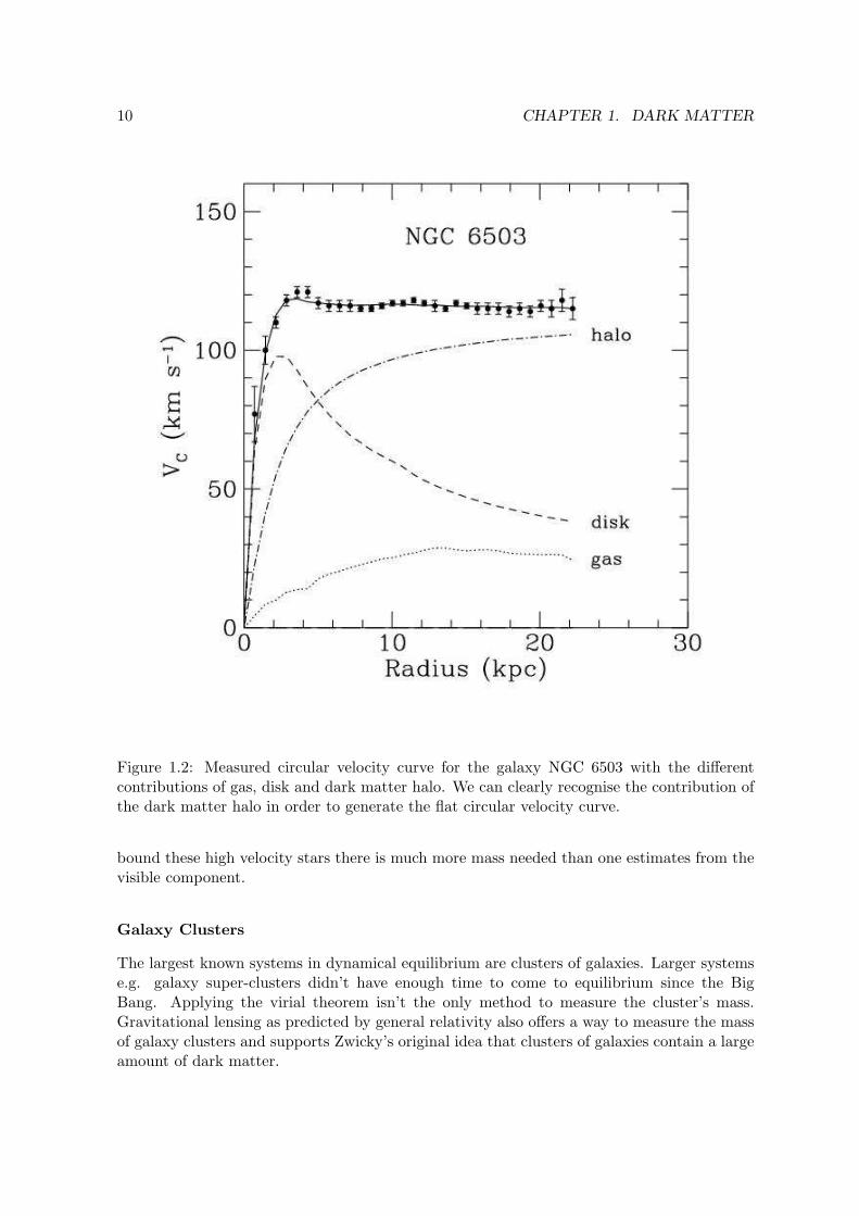
Figure 1.2: Measured circular velocity curve for the galaxy NGC 6503 with the differentcontributions of gas, disk and dark matter halo. We can clearly recognise the contribution ofthe dark matter halo in order to generate the flat circular velocity curve.
bound these high velocity stars there is much more mass needed than one estimates from thevisible component.
Galaxy Clusters
The largest known systems in dynamical equilibrium are clusters of galaxies. Larger systemse.g. galaxy super-clusters didn’t have enough time to come to equilibrium since the BigBang. Applying the virial theorem isn’t the only method to measure the cluster’s mass.Gravitational lensing as predicted by general relativity also offers a way to measure the massof galaxy clusters and supports Zwicky’s original idea that clusters of galaxies contain a largeamount of dark matter.

1.4. DARK MATTER CANDIDATES 11
1.4 Dark Matter Candidates
We have seen previously that there is a large amount of invisible dark matter in the universe.So the natural question is: What is the nature of this dark matter?
1.4.1 Estimations of the different Mass Components
Galaxy clusters represent a quite fair sample of all the different possible kinds of matter withintheir volume because they have formed from a very large region of space. From modern massestimations of clusters also using the virial theorem or gravitational lensing it is found thatΩ0
M ≈ 0.3. Since one assumes that galaxy clusters are good samples of the matter content inthe universe this is a good method to give an estimation of the fraction of Matter ΩM in theuniverse.
From observations, we know that the luminous matter content in clusters and galaxies is onlyΩ0
L ≤ 0.01. It is quite astonishing that the luminous matter contributes less than 1 % of thecritical density and only a few per cent of the total matter! So, a large fraction of the totalmass is supplied by dark matter!
The primordial nucleosynthesis gives us the possibility to estimate the baryon content Ω0B
of our universe. Combined with observational data, it is found that Ω0B ≈ 0.04. Thus, by
comparing Ω0B with Ω0
L we find that a baryonic and a non-baryonic component of dark matteris needed!
1.4.2 Classification of Dark Matter
There exist different schemes to characterise the dark matter. As we’ve seen, an obvious oneis to divide the candidates into baryonic and non-baryonic dark matter.
An other way to categorise them is by their velocity. A dark matter species is called ”hot”if it was moving at relativistic speeds at the time when it decoupled from the plasma. It iscalled ”cold” if it was moving non-relativistically at that time.
1.4.3 Baryonic Dark Matter
It is not a great surprise that baryonic dark matter should exist because we know alreadynon-luminous, baryonic dark matter e.g. planets, black holes, white dwarfs etc. Since allthese candidates are quite massive they contribute to the cold dark matter component.
MACHOs
The main baryonic candidates are the Massive Astrophysical Compact Halo Object (MA-CHO) class of candidates. The term MACHO collects a wide range of condensed baryonicmatter objects that could contribute to dark matter halos:
• White DwarfsA white dwarf is what stars like our Sun become when they have exhausted theirnuclear fuel. Near the end of its nuclear burning stage, such a star ejects most of itsouter material (creating a planetary nebula), until only the hot core remains, whichthen settles down to become a very hot (T > 100000 K) young white dwarf. A white
12 CHAPTER 1. DARK MATTER
dwarf cools down the next billion years since it has no way to keep itself hot unlessit is accreting matter from a nearby star and reaches the Chandrasekhar mass limit(≈ 1.44 M¯) and explodes in a supernova Ia.10
• Brown DwarfsBrown dwarfs are spheres of hydrogen and helium with masses below 0.08 M¯, which isthe critical mass required in order to be able to commence hydrogen burning (fusion).So they never begin nuclear fusion of hydrogen.
• PlanetsJupiter-like planets with masses ≈ 0.001 M¯ could also be dark matter candidates asmore and more extrasolar planets are discovered nowadays.
• Black HolesBlack holes with masses around a few solar masses created by the collapse of an earlygeneration of stars which were very heavy so that not much heavy elements were pro-duced are also candidates for dark matter.
In order to detect MACHOs one uses the microlensing effect. When a MACHO in the MilkyWay’s halo passes near the line of sight of a background star, it is expected from generealrelativity that the luminosity of the background star will temporarily rise. There are manycollaborations around the world that try to find such microlensing events by detecting thischaracteristic increase of the star’s luminosity curve.
Gas
From X-ray observations of elliptical galaxies one knows that many have large halos of X-rayemission. The size of these halos is a few times the optical radius of the galaxy. This X-rayflux may come from hot ionised gas which has been heated up and pushed out by some heatingmechanism (supernova heating).
X-rays were also found on galaxy cluster scales. It was discovered that clusters of galaxies areimmersed in halos of million degree gas. This hot gas is a byproduct of the galaxy formationprocess and emits large amounts of energy in the form of X-rays.
Also neutral hydrogen gas could contribute to the dark matter in the halos. But from obser-vations, we know that this delivers only a small fraction.
1.4.4 Non-baryonic Dark Matter
Particle physics provides a large number of possible candidates for non-baryonic dark matter.Most of these particles are motivated by supersymmetry, which is a theory that tries to unifygeneral relativity and quantum field theory. But also particles that are already known fromthe standard model of particle physics e.g. neutrinos are non-baryonic dark matter candidates.All these particles are often called by the term WIMPs, which stands for Weak InteractingMassive Particles.
10Since this Chandrasekhar mass limit is an universal limit for the stability of the white dwarf, one assumesthat supernova are ideal standard candles.

1.4. DARK MATTER CANDIDATES 13
Neutrino
Neutrino oscillation experiments carried out by the Super-Kamiokande group in Japan haveproved that neutrinos are massive. According to theory, Neutrinos should be changing be-tween the three neutrino types (νe, ντ and νµ) if they had mass. The experiment is executedas follows: Cosmic rays from the sun hit Earth’s atmosphere and produce muon neutrinosνµ. So, in the daytime, the detector in Japan detects these muon neutrinos νµ. However, atnight, when Japan is in darkness, the detector detects fewer muon neutrinos νµ.
Therefore, the Super-Kamiokande group concluded that during their journey through theEarth, the muon neutrinos νµ changed into tau neutrinos ντ thus proving that they havemass. Because the neutrinos are relativistic they are hot dark matter particles. But theirmass is much less than 10 eV and they are therefore ruled out as a major contribution tonon-baryonic dark matter since Ων ≈ 0.004.
Neutralino
Supersymmetry provides a huge particle zoo which contains also dark matter candidates.One of the most promissing one is the lightest stable supersymmetric particle, the neutralino.Combined arguments from accelerator searches and cosmological observations result in thefollowing mass window for the neutralino, 30 GeV < mχ < 3 TeV . Compared to the protonmass of mP = 938.3 MeV , the neutralino would be a very heavy particle and is therefore acold dark matter candidate.
Axion
Another dark matter candidate outside the standard model of particle physics is the axion.The axion arises because the QCD Lagrangian contains a term which predicts an electricdipole moment of the neutron dn = 5.2× 10⁻¹⁶θ e cm where θ is a parameter. From experi-ments, the upper limit for the neutron dipole moment is given by dn < 6.3×10⁻²⁶e cm, whichmeans θ < 10−10. So, the question is why does this θ parameter have such a small value,when it naturally would have a value near unity? This is called the strong CP problem, andone way to resolve this problem is to introduce a new Peccei-Quinn symmetry which predictsa new particle - the axion.
The axion is the Goldstone boson of the Peccei-Quinn symmetry which forces θ = 0 atlow temperatures today. At high temperatures in the early universe, the axion was mass-less. However, when the temperature of the Universe cooled below a few hundred MeV(QCD energy scale), the axion became massive. Again, combined arguments from acceleratorsearches and cosmological observations result in the following mass window for the axion,10−6eV < mA < 10−3eV . Since the axion is produced cold and never thermalized, it is agood cold dark matter candidate.

14 CHAPTER 1. DARK MATTER

Chapter 2
Modelling Dark Matter Halos
A FORTRAN program written by Stelios Kazantzidis [10] was the starting point for thisdiploma thesis. The program enables to build dark matter halos with a given density profilewhich are stable. Some fundamentals of the underlying theory that describes such a darkmatter halo are explained. These form the theoretical core of the dark matter halo generatingprogram MAKEHALO.
2.1 Statistical Mechanics and Potential Theory
2.1.1 Phase Space and Distribution Function
To describe the behaviour of a dark matter halo, we introduce a function f(x,v, t) whichgives the distribution of the dark matter particles in the phase-space Γ. It is defined, thatf(x,v, t) d3x d3v is the mass of the dark matter content within a small volume d3x d3v at thepoint (x,v) in phase-space Γ. This function is called the distribution function or phase-spacedensity and it is clear for physical reasons, that f(x,v, t) ≥ 0 everywhere in phase-space Γ.
The distribution function is a function of seven variables. If we know f(x,v, t0) at a giventime t0, we can determine the positions and velocities of the particles in our system for anytime t via Newton’s law of gravity and therefore calculate f(x,v, t) for that time t.
We write for the coordinates in phase-space Γ
(x,v) ≡ w = (w1, . . . , w6) , (2.1)
and for the velocity in phase-space Γ
w = (x, v) = (v,F) = (v,−∇Φ) , (2.2)
where F is the force per unit mass, which can be written as F = −∇Φ, where Φ is theappropriate potential as we know from potential theory.1 Such a force F is called conservative.
1If we write the force per unit mass F(x, t) = G∫
x′−x|x′−x|3 ρ(x′, t)d3x′ where G is the gravitational constant
and we define Φ(x, t) ≡ −G∫
1|x′−x|ρ(x′, t)d3x′ then the relation F = −∇Φ follows immediately from the well
known relation ∇ 1|x′−x| = x′−x
|x′−x|3 .
15

16 CHAPTER 2. MODELLING DARK MATTER HALOS
2.1.2 Collisionless Boltzmann Equation
The dark matter only interacts gravitationally and there are hardly any encounters, so thatwe can make the approximation that we can describe the dark matter as a collisionless system.The forces are conservative and therefore Liouville’s theorem holds and the volume of the flowin phase-space is conserved. The flow is described by an incompressible fluid in phase-space.
So we can write
df
dt=
∂f
∂t+
6∑
α=1
∂f
∂wαwα
=∂f
∂t+
3∑
k=1
xk
∂f
∂xk+ vk
∂f
∂vk
=∂f
∂t+ v · ∇f −∇Φ · ∂f
∂v= 0. (2.3)
Equation 2.3 is called the Collisionless Boltzmann Equation, sometimes also known as VlasovEquation. The last line holds because the system is conservative and collisionless! Thedistribution function f(x,v, t) is a solution of the Collisionless Boltzmann Equation for acollisionless system.
2.1.3 Poisson Equation
We define the mass density ρ(x, t) at the point x in real space and time t as
ρ(x, t) ≡∫
f(x,v, t)d3v. (2.4)
This is the fundamental integral equation that connects the distribution function f(x,v, t)and the density profile ρ(x, t).
The density ρ(x, t) is also related to the gravitational potential Φ(x, t) via the Poisson Equa-tion
4Φ(x, t) = 4πGρ(x, t) (2.5)
as we know again from potential theory.2
2.1.4 Steady-state Solutions
Since we’re only interested in steady-state solutions, we demand that the density profile isonly a function of x and independent of time t. One has to solve the coupled equations 2.3,2.4 and 2.5 without time dependence in order to get a solution for our system in equilibrium.Models which are based on such a solution are called self-consistent models.
Equation 2.4 relates the density ρ(x) to the distribution function f(x,v) and there are twoapproaches to generate self-consistent models, the ”f to ρ” and the ”ρ to f” approach. In the
2With the relation 4 1|x′−x| = −4πδ(x′ − x), where δ is the Dirac delta function, the Poisson Equation
follows immediately form the definition of the potential.

2.2. CUSPY HALOS 17
first method, the ”f to ρ” approach, one makes an assumption for the distribution functionf , which satisfies the Collisionless Boltzmann Equation 2.3 and calculates the density fromequation 2.4. Finally, one solves consistent equation 2.5 to get the potential Φ(x). The dis-advantage of this method is the lack of control over the resulting density profile. In the othermethod, the ”ρ to f” approach, one gives the desired density ρ(x) and calculates the poten-tial Φ(x) from the Poisson equation and gets the distribution function f(x,v) by invertingequation 2.4. Having the distribution function, it is straightforward to initialise the particlepositions and velocities. One has now the possibility to generate the N-body realization of adark matter halo. This is the approach that is used in the program MAKEHALO written byStelios Kazantzidis.
2.2 Cuspy Halos
2.2.1 Density Profile for r ≤ rvir
Studying the structure of dark matter halos analytically in the non-linear regime of the growthof gravitational instabilities is a very complex problem. Since the analytical treatment isvery difficult, many people studied the dark matter halo structure with numerical N-Bodysimulations. One is especially interested in spherical symmetric systems in equilibrium. Theresult of these studies [25], [12] showed that dark matter halos have cuspy density profileswhich can be fitted by the general formula
ρ(r) = ρ01
(rrs
)γ·(1 +
(rrs
)α)(β−γα )
, r ≤ rvir . (2.6)
The parameters α, β and γ control the slope of the profile; γ characterises the inner slope andβ the outer slope of the density profile whereas α controls the transition between the innerand outer region.
We express the r-independent parameter ρ0 as function of the critical density for closure ofthe universe ρ0
c
ρ0 ≡ δchar · ρ0c , (2.7)
with the definition of the critical density in equation 1.4 (at this epoch). We will determinethe characteristic density δchar later, which is just a dimensionless parameter.
Since we’re interested in the logarithmic slope of the profile 2.6, we calculate therefore
ln(ρ(r)) = ln(ρ0)− γ ln(
r
rs
)− β − γ
αln
(1 +
(r
rs
)α), r ≤ rvir . (2.8)
With
dr
d ln(r)=
deln(r)
d ln(r)= eln(r) = r (2.9)
we get for

18 CHAPTER 2. MODELLING DARK MATTER HALOS
d ln(ρ(r))d ln(r)
=dr
d ln(r)· d ln(ρ(r))
dr
= r ·−γ
1r− β − γ
α
α rα−1
rαs
1 +(
rrs
)α
= −γ − (β − γ)
(rrs
)α
1 +(
rrs
)α , r ≤ rvir . (2.10)
2.2.2 Scale Radius and virial Radius
We see now that the scale radius rs is the definition of locus where the transition betweenthe inner and outer slope takes place and the logarithmic slope takes the average value
d ln(ρ(r))d ln(r)
∣∣∣∣rs
= −β + γ
2. (2.11)
The virial radius rvir is defined as the distance from the centre of the dark matter halo withinwhich the mean density is ∆ times the present critical density ρ0
c . One often chooses ∆ totake on a fixed value, most common ∆ = 200. The other way is to choose ∆ to depend onthe cosmological parameters ΩM and ΩΛ according to the following relation [5]
∆(ΩM , ΩΛ) = 178 (Ω0M )0.45 (2.12)
for the case of ΩM +ΩΛ = 1 what we assume according to the concordance model of cosmology.With Ω0
M ≈ 0.3 at this epoch we obtain ∆ ≈ 103.5. In MAKEHALO, this value was used.This gives us the possibility to define the virial mass Mvir of the dark matter halo which isjust the mass within the virial radius rvir
Mvir ≡ 4π
3r3vir ∆ ρ0
c . (2.13)
We can define the scale radius rs by
rs ≡ rvir
c, (2.14)
where c is called the concentration, which is another dimensionless parameter to characterisethe dark matter halo.
2.2.3 Characteristic Density
The characteristic density δchar isn’t independent of ∆ and c and can now be determined.From
Mvir ≡ 4π
3r3vir ∆ ρ0
c = 4π
∫ rvir
0r2ρ(r)dr
= 4π δchar ρ0c
∫ rvir
0
r2
(rrs
)γ·(1 +
(rrs
)α)(β−γα )
dr (2.15)

2.2. CUSPY HALOS 19
it is easy to see that after dividing both sides by r3s and doing the substitution x ≡ r
rs, we get
for
δchar(∆, c) =∆3
c3
I(c)(2.16)
where
I(c) =∫ c
0
x2−γ
(1 + xα)(β−γ
α )dx . (2.17)
2.2.4 Density Profile for r ≥ rvir
It is obvious that density profiles with an outer slope of β > 3 describe a finite mass model.Halos with β ≤ 3 lead to a cumulative mass distribution that diverges at least logarithmi-cally. These profiles are not valid out to arbitrarily large distances and one is normally onlyinterested in the dynamics within the virial radius rvir. We need therefore to truncate thedensity profile. Instead of cutting off the density profile sharply at the virial radius rvir, wechoose an exponential cut-off that sets in at the virial radius rvir and lets the profile decayon a scale rdecay
ρ(r) = ρ01
cγ · (1 + cα)(β−γ
α )
(r
rvir
)ε
exp(−r − rvir
rdecay
), r ≥ rvir . (2.18)
The logarithm of the density is
ln(ρ(r)) = ln
(ρ0
1
cγ · (1 + cα)(β−γ
α )
)+ ε ln
(r
rvir
)− r − rvir
rdecay, r ≥ rvir (2.19)
and we get, as in a similar way before,
d ln(ρ(r))d ln(r)
= ε− r
rdecay, r ≥ rvir . (2.20)
For a smooth transition at the virial radius rvir between the inner and outer profile it isrequired that the logarithmic slope is continuous
d ln(ρ(r))d ln(r)
∣∣∣∣rvir
=−γ − βcα
1 + cα, r ≤ rvir (2.21)
d ln(ρ(r))d ln(r)
∣∣∣∣rvir
= ε− rvir
rdecay, r ≥ rvir (2.22)
and therefore
ε =rvir
rdecay− γ + βcα
1 + cα. (2.23)
20 CHAPTER 2. MODELLING DARK MATTER HALOS
2.2.5 Categories of Density Profiles
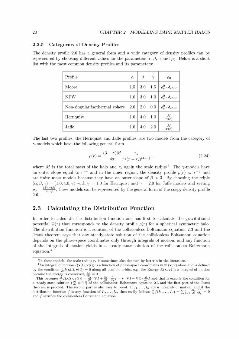
The density profile 2.6 has a general form and a wide category of density profiles can berepresented by choosing different values for the parameters α, β, γ and ρ0. Below is a shortlist with the most common density profiles and its parameters:
Profile α β γ ρ0
Moore 1.5 3.0 1.5 ρ0c · δchar
NFW 1.0 3.0 1.0 ρ0c · δchar
Non-singular isothermal sphere 2.0 2.0 0.0 ρ0c · δchar
Hernquist 1.0 4.0 1.0 M2πr3
s
Jaffe 1.0 4.0 2.0 M4πr3
s
The last two profiles, the Hernquist and Jaffe profiles, are two models from the category ofγ-models which have the following general form
ρ(r) =(3− γ)M
4π
rs
rγ(r + rs)(4−γ), (2.24)
where M is the total mass of the halo and rs again the scale radius.3 The γ-models havean outer slope equal to r−4 and in the inner region, the density profile ρ(r) ∝ r−γ andare finite mass models because they have an outer slope of β > 3. By choosing the triple(α, β, γ) = (1.0, 4.0, γ) with γ = 1.0 for Hernquist and γ = 2.0 for Jaffe models and settingρ0 = (3−γ)M
4πr3s
, these models can be represented by the general form of the cuspy density profile2.6.
2.3 Calculating the Distribution Function
In order to calculate the distribution function one has first to calculate the gravitationalpotential Φ(r) that corresponds to the density profile ρ(r) for a spherical symmetric halo.The distribution function is a solution of the collisionless Boltzmann equation 2.3 and theJeans theorem says that any steady-state solution of the collisionless Boltzmann equationdepends on the phase-space coordinates only through integrals of motion, and any functionof the integrals of motion yields in a steady-state solution of the collisionless Boltzmannequation.4
3In these models, the scale radius rs is sometimes also denoted by letter a in the literature.4An integral of motion I(x(t),v(t)) is a function of phase-space coordinates w ≡ (x,v) alone and is defined
by the condition ddt
I(x(t),v(t)) = 0 along all possible orbits, e.g. the Energy E(x,v) is a integral of motionbecause the energy is conserved, dE
dt= 0.
This becomes ddt
I(x(t),v(t)) = ∂x∂t· ∇I + ∂v
∂t· ∂
∂vI = v · ∇I −∇Φ · ∂
∂vI and that is exactly the condition for
a steady-state solution(
∂I∂t
= 0 !)
of the collisionless Boltzmann equation 2.3 and the first part of the Jeanstheorem is proofed. The second part is also easy to proof. If I1, . . . , In are n integrals of motion, and if thedistribution function f is any function of I1, . . . , In, then easily follows d
dtf(I1, . . . , In) =
∑nk=1
dIkdt
∂f∂Ik
= 0and f satisfies the collisionless Boltzmann equation.

2.3. CALCULATING THE DISTRIBUTION FUNCTION 21
Figure 2.1: Moore and NFW density profiles. The virial mass of each halo is Mvir =1012M¯/h0 corresponding to a virial radius rvir = 289.2 kpc. For each profile a concen-tration of c = 10 was used so that the scale radii match, and we get rs = 28.92. The twoprofiles have a similar outer slope of ρ(r) ∝ r−3 but differ in the central region where theMoore profile has a steeper rise ρ(r) ∝ r−1.5 whereas the NFW profile is shallower withρ(r) ∝ r−1. For r > rvir, we’re in the cut-off region.
22 CHAPTER 2. MODELLING DARK MATTER HALOS
2.3.1 Spherical Systems and Anisotropy Parameter
One of the simplest systems is a spherical one in which the two mean squared angular velocitiesare equal, v2
φ(r) = v2θ(r). The anisotropy parameter β(r) for a spherical system is defined by
β(r) ≡ 1− v2θ(r)
v2r (r)
. (2.25)
With the definition of the dispersion of the i velocity component
σ2i (r) = v2
i (r)− v2i (r) (2.26)
and assuming that the velocities are randomly distributed so that vi(r) = 0 we get
β(r) = 1− σ2θ(r)
σ2r (r)
. (2.27)
If for a spherical system, the radial velocity dispersion is equal to the each of the angularvelocity dispersions, σr = σφ = σθ then one calls the velocity dispersion tensor to be isotropic.
With σ2t ≡ σ2
φ + σ2θ = 2σ2
θ we obtain in the isotropic case
β(r) = 1− 12
σ2t (r)
σ2r (r)
. (2.28)
Hence, we expect for an isotropic velocity dispersion tensor an anisotropy parameter β = 0.
2.3.2 General Solution for an isotropic Velocity Dispersion
The distribution function f of these isotropic systems depends only on the energy per unitmass E, f = f(E). With d3v = 4πv2dv, E = 1
2v2 + Φ and dv = dEv the integral equation 2.4
becomes
ρ(r) = 4π
∫ 0
Φf(E)
√2(E − Φ) dE . (2.29)
The density ρ(r) can also be regarded as a function of Φ, ρ = ρ(Φ). Thus we see
1√8π
ρ(Φ) = 2∫ 0
Φf(E)
√E − Φ dE . (2.30)
After differentiating both sides with respect to Φ, we obtain
1√8π
dρ(Φ)dΦ
=∫ Φ
0
f(E)√E − Φ
dE = −i
∫ Φ
0
f(E)√Φ−E
dE . (2.31)
This is an Abel integral equation5 with the solution
f(E) = − 1√8π2
[∫ E
0
(d2ρ
dΦ2
)1√
Φ− EdΦ +
1√−E
(dρ
dΦ
) ∣∣∣∣∣Φ=0
], (2.32)
and was first found by Arthur Eddington in 1916.5The so called Abel integral equation a(r) =
∫ r
0
b(s)(r−s)α ds, 0 < α < 1 has the following solution
b(s) = sin(απ)π
[∫ s
0dadr
1(s−r)1−α dr + a(0)
s1−α
].

2.3. CALCULATING THE DISTRIBUTION FUNCTION 23
2.3.3 Derivatives of the Density Profile
We need therefore to calculate the first and second derivatives of the density ρ with respectto the potential Φ and express these terms as functions of the first and second derivatives ofthe density ρ with respect to r. With dΦ
dr = GM(r)r2 for a spherical symmetric system, where
M(r) denotes the mass within radius r, we get
dρ
dΦ=
dr
dΦ
(dρ
dr
)=
r2
GM(r)
(dρ
dr
). (2.33)
For the second derivative
d2ρ
dΦ2=
d
dΦ
(dρ
dΦ
)=
(d2r
dΦ2
)(dρ
dr
)+
(dr
dΦ
)2 (d2ρ
dr2
)(2.34)
we need to calculate
d2r
dΦ2=
d
dΦ
(r2
GM(r)
)
=(
dr
dΦ
)d
dr
(r2
GM(r)
)
=(
dr
dΦ
)(2rM(r)− 4πr4ρ(r)
GM2(r)
), (2.35)
where we have used ddrM(r) = d
dr
∫ r0 4πx2ρ(x)dx = 4πr2ρ(r).
We obtain now
d2ρ
dΦ2=
(d2r
dΦ2
)(dρ
dr
)+
(dr
dΦ
)2 (d2ρ
dr2
)
=(
r
GM(r)
)2 [r2
(d2ρ
dr2
)+
(2rM(r)− 4πr4ρ(r)
M(r)
)(dρ
dr
)]. (2.36)
Equation 2.36 is a general formula with the derivatives of the density profile ρ′ and ρ′′ asinput. One needs only to calculate the first and second derivative of the density profile withrespect to r.
For later convenience, we introduce the term
τ(r) ≡(
r
rs
)γ
·(
1 +(
r
rs
)α)(β−γα )
(2.37)
which is nothing else than the denominator in the density profile 2.6.
For the derivative of τ with respect to r, we obtain

24 CHAPTER 2. MODELLING DARK MATTER HALOS
dτ(r)dr
=γ
r
(r
rs
)γ
·(
1 +(
r
rs
)α)(β−γα )
+(
r
rs
)γ
·(
β − γ
α
)(1 +
(r
rs
)α)(β−γα−1) α
rs
(r
rs
)α−1
= τ(r)
γ
r+
(β − γ
rs
) (rrs
)α−1
1 +(
rrs
)α
≡ τ(r) · η(r) , (2.38)
where we made the definition
η(r) ≡ γ
r+
(β − γ
rs
) (rrs
)α−1
1 +(
rrs
)α , (2.39)
and calculating its derivative with respect to r, we obtain
dη(r)dr
= − γ
r2+
(β − γ
r2s
)(r
rs
)α−2 (α− 1)(1 +
(rrs
)α)− α
(rrs
)α
(1 +
(rrs
)α)2 . (2.40)
For the profile 2.6, we get for the first derivative in the case r ≤ rvir
dρ(r)dr
=d
dr
[ρ0
τ(r)
]
= ρ0−τ(r)η(r)
τ2(r)= −ρ(r) η(r) , r ≤ rvir . (2.41)
With
λ(r) ≡(
r
rvir
)ε
exp(−r − rvir
rdecay
)(2.42)
and its derivative
dλ(r)dr
=d
dr
[(r
rvir
)ε
exp(−r − rvir
rdecay
)]= λ(r)
[ε
r− 1
rdecay
](2.43)
we get in the case r ≥ rvir
dρ(r)dr
=d
dr
[ρ0
τ(rvir)λ(r)
]
=ρ0
τ(rvir)λ(r)
[ε
r− 1
rdecay
]
= ρ(r)[
ε
r− 1
rdecay
], r ≥ rvir . (2.44)
2.4. HALOS WITH CONSTANT DENSITY CORE 25
For the second derivative, we obtain in the case r ≤ rvir
d2ρ(r)dr2
=d
dr[−ρ(r) η(r)]
= ρ(r)η2(r)− ρ(r)dη(r)dr
= ρ(r)
[(ρ′(r)ρ(r)
)2
− dη(r)dr
], r ≤ rvir , (2.45)
and for the case r ≥ rvir
d2ρ(r)dr2
=d
dr
[ρ(r)
[ε
r− 1
rdecay
]]
= ρ(r)[
ε
r− 1
rdecay
]2
− ρ(r)ε
r2
= ρ(r)
[(ρ′(r)ρ(r)
)2
− ε
r2
], r ≥ rvir . (2.46)
We can now have a closer look at the solution 2.32 for our distribution function. We see thatdρdΦ
∣∣Φ=0
= 0 for our density profiles. The remaining integral will be evaluated numerically.
2.4 Halos with constant Density Core
2.4.1 Density Profile
How could one modify the density profile 2.6 in order to get a core with constant densitywithin a so called core radius without loosing the outer characteristics of the density profile?The simplest answer is, that we just add a constant κ in the denominator of the density profile2.6. Thus, our density profile for a halo with constant density core looks like
ρ(r) =ρ0
τ(r) + κ, r ≤ rvir , (2.47)
and in the cut-off region
ρ(r) =ρ0
τ(rvir) + κλ(r) , r ≥ rvir . (2.48)
Here we will also use the abbreviation terms τ(r) 2.37, η(r) 2.39 and λ(r) 2.42 introducedearlier in this chapter.
How does one define the core radius? This question leads to a related question. Where willκ become important. This question is easy to answer. The κ-term becomes important whenit is as large as the τ -term, τ(r) ≈ κ. So we define the core radius rcore by the relation
κ ≡ τ(rcore) . (2.49)

26 CHAPTER 2. MODELLING DARK MATTER HALOS
2.4.2 Distribution Function
We saw in equation 2.36, that its only input are the first and second derivatives of the densityprofile with respect to r. We need therefore again to calculate these expressions.
In the case r ≤ rvir, for first derivative of the density profile 2.47 we obtain
dρ(r)dr
=d
dr
[ρ0
τ(r) + κ
]
= ρ0−τ(r)η(r)[τ(r) + κ]2
= −ρ(r)τ(r)
τ(r) + κη(r) , r ≤ rvir , (2.50)
and for the case r ≥ rvir
dρ(r)dr
=d
dr
[ρ0
τ(rvir) + κλ(r)
]
=ρ0
τ(rvir) + κλ(r)
[ε
r− 1
rdecay
]
= ρ(r)[
ε
r− 1
rdecay
], r ≥ rvir . (2.51)
If we want again a smooth transition at the virial radius rvir, we obtain for
dρ(r)dr
∣∣∣∣rvir
= −ρ(rvir)τ(rvir)
τ(rvir) + κη(rvir) , r ≤ rvir , (2.52)
dρ(r)dr
∣∣∣∣rvir
= ρ(rvir)[
ε
rvir− 1
rdecay
], r ≥ rvir , (2.53)
and therefore for
ε =rvir
rdecay− rvir
τ(rvir)τ(rvir) + κ
η(rvir) =rvir
rdecay− τ(rvir)
τ(rvir) + κ
[γ + βcα
1 + cα
]. (2.54)
For the second derivative, we calculate
d2ρ(r)dr2
=d
dr
[−ρ(r)
τ(r)τ(r) + κ
η(r)]
= ρ(r)(
τ(r)τ(r) + κ
η(r))2
− ρ(r)τ ′(r)[τ(r) + κ]− τ(r)τ ′(r)
[τ(r) + κ]2η(r)
−ρ(r)τ(r)
τ(r) + κη′(r)
= ρ(r)τ(r)
[τ(r) + κ]2[τ(r)η2(r)− κη2(r)− τ(r)η′(r)− κη′(r)
], r ≤ rvir ,(2.55)

2.4. HALOS WITH CONSTANT DENSITY CORE 27
and
d2ρ(r)dr2
=d
dr
[ρ(r)
[ε
r− 1
rdecay
]]
= ρ(r)[
ε
r− 1
rdecay
]2
− ρ(r)ε
r2
= ρ(r)
[(ρ′(r)ρ(r)
)2
− ε
r2
], r ≥ rvir . (2.56)
A little cross check shows, that all the results are compatible with the previous deduced resultsfor the density profile without core. By setting κ = 0, all the expressions calculated in thissection reduce to the normal results we’ve calculated for the density profile without core 2.6.
2.4.3 Characteristic Density
We now only need to calculate the new expression for the characteristic density δchar in thecase of the density profile for a core 2.47. From
Mvir ≡ 4π
3r3vir ∆ ρ0
c = 4π
∫ rvir
0r2ρ(r)dr
= 4π δchar ρ0c
∫ rvir
0
r2
(rrs
)γ·(1 +
(rrs
)α)(β−γα )
+ κ
dr (2.57)
it is easy to see that again after dividing both sides by r3s and doing the substitution x ≡ r
rs,
we get for
δchar(∆, c) =∆3
c3
I(c)(2.58)
where now
I(c) =∫ c
0
x2
xγ (1 + xα)(β−γ
α ) + κdx . (2.59)

28 CHAPTER 2. MODELLING DARK MATTER HALOS

Part II
Simulations
29


Chapter 3
Shell Model Halos
With the wish to get a higher resolution in the inner region of a dark matter halo where wewanted to study the stability of the cusp slope, the idea of dividing the halo into differentshells was born. For each shell one should be able to choose the number of particles and onecan in this way choose the needed resolution in the shell. Hence, the first step was to modifythe original code by Stelios Kazantzidis [10].
The code was modified in the following way. One could in maximum have 3 shells:
shell 1 rmin ≤ r ≤ rshell1
shell 2 rshell1 < r ≤ rshell2
shell 3 rshell2 < r
By either setting rshell1 = 0 or setting both shell radii to 0, one could also choose 2 or 1 shellmodels. Thus, this code also produces halos without shells as the original code did.
By choosing the number of particles in each shell, one could have the requested resolutione.g. high resolution with a lot of particles in the centre (shell 1) and a low resolution in theouter region with fewer particles (shell 3). By choosing an individual gravitational softeninglength for the particles in each shell, we prevent to the effect that heavy particles kick outthe lighter particles.
3.1 Initial Conditions
3.1.1 Dark Matter Halo
We set up a dark matter halo with a Moore profile and virial mass Mvir = 1012M¯. The shellradii were rshell1 = 2 kpc respectively rshell2 = 50 kpc and we had 200000 particles in the firstshell, 70000 particles in the second shell and 30000 particles in the third shell.
The gravitational softening was for the light particles in shell 1 ε1 = 0.1 kpc, for the mediummass particles ε2 = 1 kpc and for the heavy particles ε3 = 10 kpc. We call this model HALOA and further details can be seen in the appendix D.1.
3.2 Simulation and Results
The main interest was if this shell model is stable. So, we let it evolve with PKDGRAV andchose a time step ∆t = 0.1 Gyr.
31

32 CHAPTER 3. SHELL MODEL HALOS
Figure 3.1: (left) Density profile of shell model HALO A with different softenings. (right)Density profile for HALO A with equal softenings for all particles.
3.2.1 Stability
What we can clearly see in figure 3.1 is that in the case with different softenings, the centraldensity drops by nearly a factor of 5! In order to rule out an effect of the larger softenings ofthe medium and heavy mass particles, we performed a simulation of the same model but withequal softenings. In that case, even more particles are scattered out by the heavy particlesthat are now more pointlike due to the smaller softening.
It is not that clear in detail why the shell model failed, but since we wanted to create a modelthat is at least stable from a few softening length on, we dropped the idea of the shell modelhalo and worked form now on with single mass models.

Chapter 4
Sinking Black Hole
Does a sinking black hole produce a constant density core? That’s the question we would liketo answer here. In this simulation, we let a black hole sink to the centre of the equilibriumdark matter halo and investigate how this perturbation affects the density profile of the darkmatter halo.
4.1 Initial Conditions
4.1.1 Dark Matter Halo
We choose a Moore profile for the halo with a concentration of c=7.5 and a virial massMvir = 1012 M¯. The total number of particles in the halo is 2 × 10⁶ and a softening ofεDM = 0.1 kpc was chosen for the dark matter particles. Let’s call this halo HALO B.Further details can be seen in D.2.
4.1.2 Black Hole
The black hole had a mass of MBH = 107 M¯ and the gravitational softening of the blackhole was also εBH = 0.1 kpc.
Two simulations were performed. In each of these two simulations, the black hole was setinto the dark matter halo at the position xBH = (0, 1, 0) kpc where the point (0,0,0) is thecentre of the dark matter halo. In the first simulation, the black hole had a velocity ofvBH1 = (90, 0, 0) km s−1 which corresponds to the circular velocity at the radius r = 1 kpcfor HALO B, vc(1 kpc) ≈ 90 km s−1. For the second version, we chose half the velocity vectorof version 1 vBH2 = (45, 0, 0) km s−1
4.2 Simulation and Results
The time evolution was executed with PKDGRAV and a time step of ∆t = 0.1 Gyr waschosen.
33

34 CHAPTER 4. SINKING BLACK HOLE
4.2.1 Dynamical Friction Time
Due to the effect of dynamical friction1, the black hole sinks to the centre where we have thedeepest potential well. So, the time when the black hole reaches the centre and stays therehad to be determined.
For the first simulation with the fast black hole (vBH1 = (90, 0, 0) km s−1), the dynamical fric-tion time tf1 ≈ 1.3 Gyr was found and for the slower black hole with vBH2 = (45, 0, 0) km s−1,we got tf2 ≈ 0.5 Gyr.
4.2.2 Evolution of Density Profiles and Anisotropy Parameters
We were especially interested in the change of the density slope in the central region r < 1 kpc.What is the effect of the black hole while it is spiralling in and to what degree will the densityprofile change after the black hole reached the centre? We plotted therefore the initial densityprofile, the profile after the dynamical friction time tf1 respectively tf2 and after 1.5 Gyr afterthe black hole reached the centre.
Figure 4.1: (left) Density profiles for the fast black hole vBH1 = (90, 0, 0) km s−1. (right)Density profiles for the slow black hole vBH2 = (45, 0, 0) km s−1. In each case, the initialprofile, the profile after the dynamical friction time tf1 = 1.3 Gyr respectively tf2 = 0.5 Gyrand after tf1 + 1.5 Gyr = 2.8 Gyr respectively tf2 + 1.5 Gyr = 2.0 Gyr is presented.
We observe in both cases a flattening of the density profile in the very central region. Sincethis might also be an effect of the low resolution (although we used 2× 10⁶ particles for thehalo) or an effect of the softening or any other parameter we don’t have under control, weperformed a reference run of the halo without sinking black hole in order to test the stability.See chapter 4.2.3 for the results.
1The motion of a massive body in a sea of matter produces an overdensity of matter behind the body whichleads to a deceleration of the body due to the higher gravitational force from behind. This effect is calleddynamical friction.

4.2. SIMULATION AND RESULTS 35
We also investigated the change of the anisotropy parameter β(r). In the central region, weobserve no relevant change than the usual fluctuations already present in the initial conditionsmost likely due to low resolution. But an increase of the anisotropy parameter in the outerregion made us very suspicious since this was not expected from simulations performed pre-vious [10]. What is the effect of this shift in the velocity structure to more radial velocities?This was also a reason to do a reference simulation in order to see if the black hole is involvedin this effect or not.
Figure 4.2: Evolution of the Anisotropy parameter for the fast black hole (left) and the slowblack hole (right). In the central part, we have some fluctuations already present in theinitial conditions (IC). But in the outer region, the anisotropy parameter increases due tounexpected reasons.
4.2.3 Stability
For several reasons as mentioned above, we performed a reference run of the single halo weused for the sinking black hole experiment. There was no change in the parameters of thesimulation. The only difference to the previous simulations was that the black hole wasremoved form the initial conditions.
We observed, that the change in the density profile in the central region is very large and thatthe halo is more or less stable beyond ≈ 5 × εDM . So we can’t do any statement about theeffect of the sinking black hole. What we see is, that in the case of the halo with black hole,the flattening isn’t that large. So, the simulations with the black hole are even more stable.We don’t know at the moment if the black hole is really responsible for this better stabilityof the halos at the centre.
In the outer region of the halo, we observe an increase in the density profile between 10 kpc−200 kpc and a stronger cut-off around 300 kpc. Since we also observe an kinetic energyof the total system that is approximately 10 % to low, we assume that this change of the

36 CHAPTER 4. SINKING BLACK HOLE
Figure 4.3: Density profile (left) and and anisotropy parameter (right) for the reference runin order to test the stability. We can clearly see that we can’t rely on the central part of ourdensity profiles.
density profile is due to infalling material. This is also supported by the observed increase ofthe anisotropy parameter in exact the same range. Due to the infall, the velocity structuredeparts from the initial isotropic case to a more radial velocity structure.
The conclusion form this reference run is, that we can’t observe an effect of the black holesince we have larger effects from the evolution of the single halo. This little instabilities ofthe halo may have different reasons as already mentioned above. But also some bad choice ofparameters for the simulation could have caused some effects. This is sill a topic for furthertests.

Chapter 5
Merger Sequence
In a sequence of mergers of dark matter halos with different central density profile slopesand each halo containing a central massive black hole, we investigated how the merger timedepends on the slope and how the density profile changes.
5.1 Initial Conditions
5.1.1 Dark Matter Halo
We started with a Moore profile halo with (α, β, γ) = (1.5, 3.0, 1.5), fixed α and β for theother halos and changed only the central slope γ:
Halo name (α, β, γ)
HALO C (1.5,3.0,1.5)
HALO D (1.5,3.0,1.0)
HALO E (1.5,3.0,0.5)
HALO F (1.5,3.0,0.0)
The virial mass of each halo was Mvir = 1012M¯ which gives a virial radius rvir = 289.2 kpc.The concentration cγ of each halo was chosen so, that the radius where the maximum circularvelocity is reached, rvcm, is the same for each halo. This was done empirically. From the halocreating program, we produced the circular velocity curve for each halo profile with equalconcentration c = 7.5 and therefore equal scale radius rs = 38.56 kpc and ruled out the rvcm:
γ = 1.5 rvcm = 48.20 kpc = 1.25 rs
γ = 1.0 rvcm = 79.70 kpc = 2.07 rs
γ = 0.5 rvcm = 106.35 kpc = 2.76 rs
γ = 0.0 rvcm = 129.70 kpc = 3.36 rs
This can also be verified in figure 5.1. If we choose for HALO D a concentration of c1.0 = 10,we obtain the following concentrations cγ :
c1.5 = 6.04 c1.0 = 10.0 c0.5 = 13.4 c0.0 = 16.2 (5.1)
37

38 CHAPTER 5. MERGER SEQUENCE
Figure 5.1: (left) Halo profiles with equal contentration c = 7.5. The virial mass was Mvir =1012M¯ corresponding to a virial radius rvir = 289.2 kpc and therefore to a scale radiusrs = 38.56 kpc. (right) Halo profiles now with concentrations according to equation 5.1. Themaximum circular velocity is reached for each profile at rvcm ≈ 60 kpc.
These concentrations were used for HALO C to HALO F and the resulting circular velocitycurve can be seen in figure 5.1.
Since this empirical result wasn’t quite satisfying, an exact calculation was performed. Un-fortunately this was done after the simulations have started already. The details and resultsof this calculation can be found in the appendix in equation B.24. But the empirically foundrelation 5.1 and the exact results B.24 agree quite good.
In order to get more particles near the centre, the number of particles was also increased forshallower profiles. The gravitational softening of the dark matter particles was in each halothe same, εDM = 0.1 kpc. More details on the specific halo parameters can be found in theappendix D.3 to D.6.
5.1.2 Black Hole
The black hole in the centre of each halo had a mass of MBH = 107M¯ and was set in withoutvelocity. The softening of the black hole was chosen also to be εBH = 0.1 kpc.
5.1.3 Merger Set-up
In each merger, we put in two halos with a central black hole. The first halo (with blackhole) was set in at x1 = (0, 0, 0) kpc and the second one at x2 = (0, 500, 0) kpc. So, they wereinitially separated by 500 kpc. The velocity of the first halo was v1 = (0, 0, 0) km s−1 andthe second halo had v2 = (0,−150, 50) km s−1 ≈ (0,−vc(rvir), 1
3vc(rvir)). This was for eachof the four mergers the same.

5.2. SIMULATION AND RESULTS 39
5.2 Simulation and Results
For the time step in the PKDGRAV, ∆t = 0.01 Gyr was chosen in order to get a niceresolution of the paths of the black holes spiralling around each other.
5.2.1 Black Hole Separation
In figure 5.2 we plotted the separation of the two black holes versus time. For the cases ofγ = 1.5 and γ = 1.0, we let it evolve for 6 Gyr and in the other two cases, the simulationtime was 8 Gyr.
As we actually expect, we can clearly recognise form figure 5.2, that for the very first encounterof the black holes, the central slope of the density profile doesn’t play any role. We find forthe time of the first minimal approach tfa and the separation dfa:
γ = 1.5 tfa = 1.99 Gyr dfa = 32.31 kpc
γ = 1.0 tfa = 1.99 Gyr dfa = 31.73 kpc
γ = 0.5 tfa = 1.99 Gyr dfa = 32.47 kpc
γ = 0.0 tfa = 1.99 Gyr dfa = 31.81 kpc
So, for all mergers, the first approach happens after tfa = 1.99 Gyr and the black holes areroughly separated by dfa ≈ 32 kpc. The detailed internal structure plays only a role for latertimes when the halos ”feel” the different central density slope.
The orbits of the black holes decay more rapidly the steeper the central density profile is dueto dynamical friction. In the cases of γ = 1.5 and γ = 1.0 we can even define a merger time ofthe black holes tbm. See section 5.2.3 for further details. If one wants to analyse the mergerprocess in detail, one has to start with a better resolution and smaller softening lengths or onehas to use a refined simulation in a later stage of the simulation. Due to the large softening inour simulation, the black holes scatter around and have approximately an average separationof d ≈ 0.5 kpc.
But for the two shallow profiles with γ = 0.5 and γ = 0.0, the black holes oscillate in the largecore established by the merging process. They never come close enough that they will evermerge once! This has an important consequence. If supermassive black holes are really theproduct of mergers of black holes, then the central halo density profile mustn’t be γ ≤ 0.5!
5.2.2 Halo Merger Time
How do we define the point in time when the two halos have merged? We defined the halomerger time thm by the the time of the first minimal approach of the black holes after whichthe density profile is stable for distances larger than 1 kpc. We found the following mergertimes:
γ = 1.5 thm = 4.55 Gyr
γ = 1.0 thm = 5.01 Gyr
γ = 0.5 thm = 6.15 Gyr
γ = 0.0 thm = 5.51 Gyr

40 CHAPTER 5. MERGER SEQUENCE
The shallower the central density profile is, the longer it takes the two halos to merge. Thisgeneral tendency is is not valid in the case of a complete flat central density profile. Here,the merged halos reache relatively early an equilibrium state.
5.2.3 Black Hole Merger Time
We’ve chosen a softening length εBH = 0.1 kpc for the black holes. That means that they inaverage never come closer than approximately the softening length in our simulation. Hence,we define the black hole merger time tbm by the first minimal separation of the black holeswhere we found before a maximum separation smaller than 0.5 kpc. With this definition, wefind in the case of the two most steepest central density profiles:
γ = 1.5 tbm = 4.72 Gyr
γ = 1.0 tbm = 5.82 Gyr
For the other two cases we couldn’t define a black hole merger time this way. Actually, theywill never merge since they are wandering around in the large core with a flat density profileestablished by the merger.
5.2.4 Evolution of Density Profiles
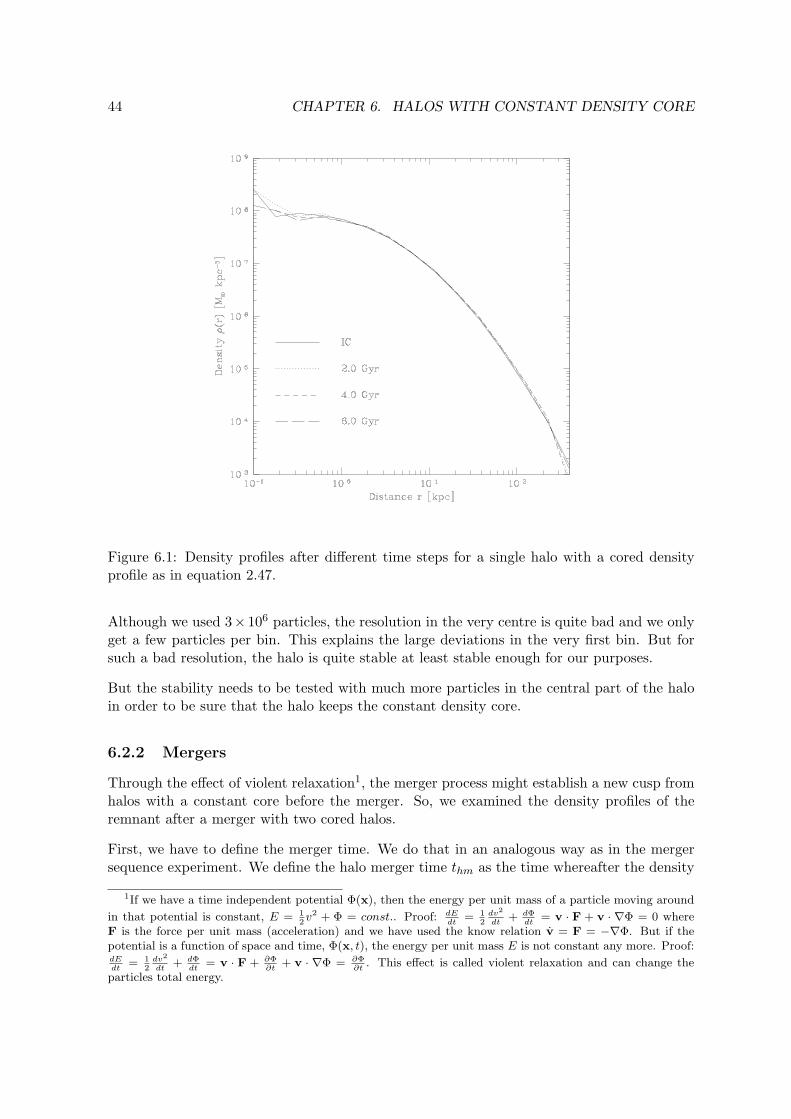
A very interesting question is: What happens with the density profile? In figure 5.3 we haveplotted the density profiles for each merger after the halo merger time thm defined in section5.2.2.
In all the profiles with a non-zero γ, we see a clear flattening of the density profile. Since thesingle halos are only stable beyond a few softening lengths, we can’t rely on the profile in thevery centre. But there is a clear tendency for flatter profiles after the merger.
By the shift of the density profile curve after the merger compared to the initial halo densityprofile, we see that the volume in phase-space is quite well conserved. The shift correspondsapproximately to the factor two (log10(2) ≈ 0.3) in more mass in a given phase-space volumed3x d3v. At least in the outer part of the density profile, this seems to be true whereas wesee the deviations in the central part due to the flattening of the profile.

5.2. SIMULATION AND RESULTS 41
Figure 5.2: Separation of the black holes for the different density profiles. In the cases ofγ = 1.5 and γ = 1.0, the black holes will merge after 4.72 Gyr respectively 5.82 Gyr. In theother two cases the black holes won’t merge. Please also notice the different time scales ofthe upper and lower plots.

42 CHAPTER 5. MERGER SEQUENCE
Figure 5.3: Density profiles of the finally merged dark matter halos. The initial densityprofiles (IC) of the two halos are compared with the profiles of the merged halos after thehalo merger time thm defined in section 5.2.2.

Chapter 6
Halos with constant Density Core
We created halos with a constant density core with a profile 2.47. First, their stability wasexamined and later two merger between two cored halos were performed to see if through themerger process a new cusp is produced.
6.1 Initial Conditions
6.1.1 Dark Matter Halo
In order to create halos with a density profile 2.47, the original code of MAKEHALO had tobe modified. With the modified program, we created a halo with outer density characteristicslike the Moore profile (1.5,3.0,1.5). The core radius, as defined in 2.49, was set to rcore = 2 kpc.The virial mass was Mvir = 1012 M¯ and in total we had 3 × 10⁶ particles. The softeninglength of the dark matter particles was εDM = 0.1 kpc. We call this halo model HALO Gand further details can be seen in appendix D.7.
6.1.2 Merger Set-up
We set up two merger scenarios. The first merger consited of two HALO G halos and wasset up the following way: we set in the first halo at x1 = (0, 0, 0) kpc and the second was setin 500 kpc apart at x2 = (0, 500, 0) kpc. The velocities were again v1 = (0, 0, 0) km s−1 andv2 = (0,−150, 50) km s−1. So, the initial conditions had angular momentum.
The second merger had the same initial positions but different velocities: v1 = (0, 0, 0) km s−1
and v2 = (0,−150, 0) km s−1. The second halo is heading directly to the first one.
6.2 Simulation and Results
For the time evolution with PKDGRAV, a time step of ∆t = 0.1 Gyr was used.
6.2.1 Stability
The first test of course was a stability test: How stable are these cored halos? We let thereforea single model G halo evolve for 6 Gyr.
43
44 CHAPTER 6. HALOS WITH CONSTANT DENSITY CORE
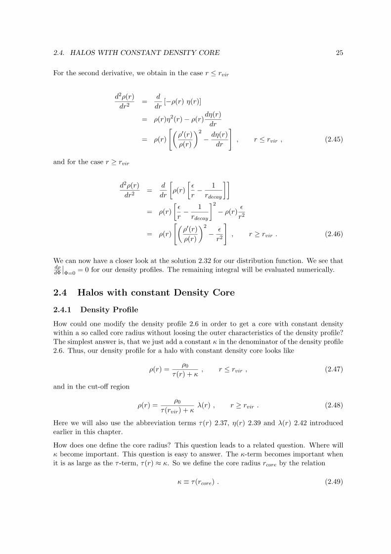
Figure 6.1: Density profiles after different time steps for a single halo with a cored densityprofile as in equation 2.47.
Although we used 3× 10⁶ particles, the resolution in the very centre is quite bad and we onlyget a few particles per bin. This explains the large deviations in the very first bin. But forsuch a bad resolution, the halo is quite stable at least stable enough for our purposes.
But the stability needs to be tested with much more particles in the central part of the haloin order to be sure that the halo keeps the constant density core.
6.2.2 Mergers
Through the effect of violent relaxation1, the merger process might establish a new cusp fromhalos with a constant core before the merger. So, we examined the density profiles of theremnant after a merger with two cored halos.
First, we have to define the merger time. We do that in an analogous way as in the mergersequence experiment. We define the halo merger time thm as the time whereafter the density
1If we have a time independent potential Φ(x), then the energy per unit mass of a particle moving around
in that potential is constant, E = 12v2 + Φ = const.. Proof: dE
dt= 1
2dv2
dt+ dΦ
dt= v · F + v · ∇Φ = 0 where
F is the force per unit mass (acceleration) and we have used the know relation v = F = −∇Φ. But if thepotential is a function of space and time, Φ(x, t), the energy per unit mass E is not constant any more. Proof:dEdt
= 12
dv2
dt+ dΦ
dt= v · F + ∂Φ
∂t+ v · ∇Φ = ∂Φ
∂t. This effect is called violent relaxation and can change the
particles total energy.
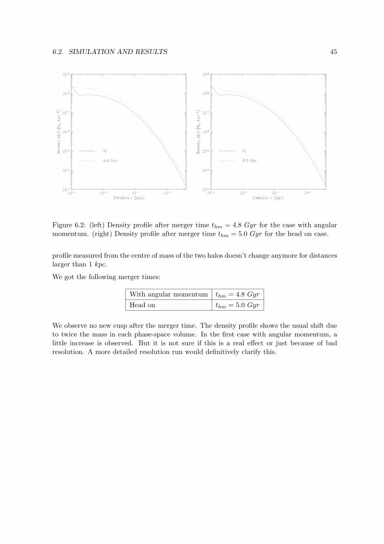
6.2. SIMULATION AND RESULTS 45
Figure 6.2: (left) Density profile after merger time thm = 4.8 Gyr for the case with angularmomentum. (right) Density profile after merger time thm = 5.0 Gyr for the head on case.
profile measured from the centre of mass of the two halos doesn’t change anymore for distanceslarger than 1 kpc.
We got the following merger times:
With angular momentum thm = 4.8 Gyr
Head on thm = 5.0 Gyr
We observe no new cusp after the merger time. The density profile shows the usual shift dueto twice the mass in each phase-space volume. In the first case with angular momentum, alittle increase is observed. But it is not sure if this is a real effect or just because of badresolution. A more detailed resolution run would definitively clarify this.

46 CHAPTER 6. HALOS WITH CONSTANT DENSITY CORE

Part III
Appendix
47


Appendix A
Some useful astrophysical Constants
Speed of Light (exact) c ≡ 2.99792458× 10⁸ m s−1
Year yr = 3.156× 10⁷ s
Light-year lyr ≡ c · yr
= 9.461× 10¹⁵ m
Astronomical Unit AU = 1.496× 10¹¹ m
Parsec pc ≡ AU/ tan(1′′)= 3.086× 10¹⁶ m
= 3.262 lyr
Solar Mass M¯ = 1.989× 1030 kg
Solar Luminosity L¯ = 3.826× 1026 J s−1
Gravitational Constant G = 6.672× 10⁻¹¹ m3 s−2 kg−1
= 4.301× 10⁻⁶ km2 s−2 kpc M−1¯
Hubble Parameter H = 100× h km s−1 Mpc−1
Critical Density ρc ≡ 3H2
8πG
= 1.879× 10⁻²⁶ h2 kg m−3
= 277.6× h2 M¯ kpc−3
49

50 APPENDIX A. SOME USEFUL ASTROPHYSICAL CONSTANTS

Appendix B
Where is the maximum circularVelocity reached?
One is often interested where for a given density profile the maximum circular velocity isreached. This will happen at a radius rvcm. We will investigate how this radius rvcm isrelated to other characteristic distances in the profile and derive a relation between rvcm andthe scale radius rs.
B.1 Criteria for maximum circular Velocity
As we saw previously in equation 1.23, the circular velocity is defined by
vc(r) ≡√
GM(r)r
. (B.1)
Taking the derivative of the square of this equation, we get
2vc(r)dvc(r)
dr=
GM ′(r)r −GM(r)r2
. (B.2)
With the condition for an extremum, dvc(r)dr
∣∣∣rvcm
= 0, we obtain
M(rvcm) = M ′(rvcm)rvcm (B.3)
and therefrom
1 =d ln(M(r))
d ln(r)
∣∣∣∣rvcm
. (B.4)
By using again M ′(r) = ddrM(r) = d
dr
∫ r0 4πx2ρ(x)dx = 4πr2ρ(r), the following alternative
condition can be derived∫ rvcm
0x2ρ(x)dx = ρ(rvcm)r3
vcm , (B.5)
where ρ(r) denotes the density profile. This equation is not that simple to solve in generaland we concentrate therefore on the special cases of a Moore and a NFW profile in order tocalculate the integral on the left side with the mathematical software tool Maple.
51
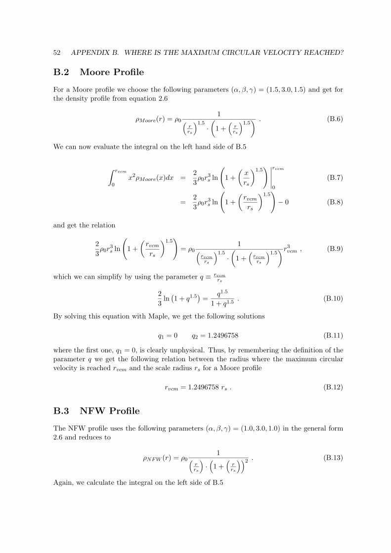
52 APPENDIX B. WHERE IS THE MAXIMUM CIRCULAR VELOCITY REACHED?
B.2 Moore Profile
For a Moore profile we choose the following parameters (α, β, γ) = (1.5, 3.0, 1.5) and get forthe density profile from equation 2.6
ρMoore(r) = ρ01
(rrs
)1.5·(
1 +(
rrs
)1.5) . (B.6)
We can now evaluate the integral on the left hand side of B.5
∫ rvcm
0x2ρMoore(x)dx =
23ρ0r
3s ln
(1 +
(x
rs
)1.5)∣∣∣∣∣
rvcm
0
(B.7)
=23ρ0r
3s ln
(1 +
(rvcm
rs
)1.5)− 0 (B.8)
and get the relation
23ρ0r
3s ln
(1 +
(rvcm
rs
)1.5)
= ρ01
(rvcmrs
)1.5·(
1 +(
rvcmrs
)1.5)r3
vcm , (B.9)
which we can simplify by using the parameter q ≡ rvcmrs
23
ln(1 + q1.5
)=
q1.5
1 + q1.5. (B.10)
By solving this equation with Maple, we get the following solutions
q1 = 0 q2 = 1.2496758 (B.11)
where the first one, q1 = 0, is clearly unphysical. Thus, by remembering the definition of theparameter q we get the following relation between the radius where the maximum circularvelocity is reached rvcm and the scale radius rs for a Moore profile
rvcm = 1.2496758 rs . (B.12)
B.3 NFW Profile
The NFW profile uses the following parameters (α, β, γ) = (1.0, 3.0, 1.0) in the general form2.6 and reduces to
ρNFW (r) = ρ01(
rrs
)·(1 +
(rrs
))2 . (B.13)
Again, we calculate the integral on the left side of B.5

B.4. CONCENTRATION RELATION 53
∫ rvcm
0x2ρNFW (x)dx = ρ0
(r4s
rs + x+ r3
s ln(rs + x)) ∣∣∣∣∣
rvcm
0
(B.14)
= ρ0
(r4s
rs + rvcm+ r3
s ln(rs + rvcm)− r3s − r3
s ln(rs))
(B.15)
and derive the following relation
ρ0
(r4s
rs + rvcm+ r3
s ln(rs + rvcm)− r3s − r3
s ln(rs))
= ρ01(
rvcmrs
)·(1 +
(rvcmrs
))2 r3vcm (B.16)
which we can also simplify by using the q ≡ rvcmrs
parameter and dividing by r3s
11 + q
+ ln(rs) + ln(1 + q)− 1− ln(rs) =q2
(1 + q)2(B.17)
leading to
ln(1 + q) =q + 2q2
(1 + q)2. (B.18)
We calculate the solutions again with Maple and obtain
q1 = 0 q2 = 2.1625816 (B.19)
where the first one, q1 = 0, is again unphysical. Thus, we get the following relation betweenthe radius where the maximum circular velocity is reached rvcm and the scale radius rs for aNFW profile
rvcm = 2.1625816 rs . (B.20)
B.4 Concentration Relation
If one wants now to scale a Moore profile and a NFW profile with the same virial mass andthus have equal virial radii rvir for both halos so that the radii where the maximum circularvelocity is reached are the same, we get a condition for the associated concentrations.
From the equality of
rvcm,1 = α1rs,1 = α2rs,2 = rvcm,2 (B.21)
we get witch ci ≡ rvirrs,i
α1
α2=
rs,2
rs,1=
c1
c2. (B.22)
With α1 = 1.2496758 and α2 = 2.1625816 we obtain the relation between the concentrationof the Moore and a NFW profiles so that the profiles match at the maximum circular velocity
cMoore ≈ 0.5779 cNFW (B.23)

54 APPENDIX B. WHERE IS THE MAXIMUM CIRCULAR VELOCITY REACHED?
Figure B.1: Circular velocity curve for a Moore and a NFW profile. The virial mass of eachhalo is Mvir = 1012M¯/h0 corresponding to a virial radius rvir = 289.2 kpc (locus wherethe two curves intersect). For the NFW profile a concentration of cNFW = 10 was used andaccording to B.23 a concentration of cMoore = 5.8 was used for the Moore profile. Hence, themaximum circular velocity is reached for both profiles at rvcm ≈ 62 kpc.
B.5 Merger Sequence - Exact Results
For the sequence of mergers with the profiles (1.5, 3.0, γ) where γ takes the values γ = 1.5,1.0, 0.5, 0.0 the relation between the locus where the maximum circular velocity is reachedrvcm and the scale radius rs were calculated in a similar way as before:
Profile Relation(1.5, 3.0, 1.5) rvcm = 1.2496758 rs
(1.5, 3.0, 1.0) rvcm = 2.0549297 rs
(1.5, 3.0, 0.5) rvcm = 2.7473910 rs
(1.5, 3.0, 0.0) rvcm = 3.3712527 rs
If we choose for the nearly NFW profile (1.5,3.0,1.0) a concentration of c1.0 = 10, we obtain
c1.5 = 6.081 c1.0 = 10.00 c0.5 = 13.37 c0.0 = 16.41 (B.24)

Appendix C
Software Tools
C.1 Available Software
C.1.1 MAKEHALO
This program was written by Stelios Kazantzidis and provides a tool for creating stableequilibrium halos with density profile 2.6 for an arbitrary choice of the parameters (α, β, γ).All the halos used in this diploma thesis were created by using MAKEHALO or a littlemodified version for creating halos with density profile 2.47. The theoretical fundamentals ofthis program are presented in chapter 2. A detailed description of the code and stability testsof halos can be found in [10].
C.1.2 PKDGRAV
To evolve the simulations in time the program PKDGRAV which stands for Parallel K-Dtree GRAVity was used. This program was written by Joachim Stadel and Thomas Quinnand is a state-of-the-art, multi-stepping, parallel N-body code.
C.1.3 TIPSY
TIPSY (Theoretical Image Processing SYstem) is a program written by Neal Katz andThomas Quinn and is able to visualise, manipulate and analyse N-body systems. It wasmainly used to create density profiles of dark matter halos and produce movies of dark matterhalo mergers.
Along with TIPSY come some nice programs as totipnat, totipstd, ascii2bin and bin2ascii inorder to convert human readable ASCII-files into Tipsy readable bin- or std-files for example.
More details can be found on:http://www-hpcc.astro.washington.edu/tools/tipsy/tipsy.html
C.1.4 Super Mongo
Super Mongo is a nice program written by Robert Lupton and Patricia Monger to createplots. All the plots in this document were produced with Super Mongo.
More details can be found on:http://www.astro.princeton.edu/∼rhl/sm/
55

56 APPENDIX C. SOFTWARE TOOLS
C.2 Self-written Programs
C.2.1 Composeascii
Composeascii is a little FORTRAN program that adds two Tipsy-ASCII-files. One can choosea shift in space and velocity of the second system with respect to the first one. This programwas mainly used to set black holes into dark matter halos or creating the merger set-ups.
C.2.2 Readstarxv
This C-program program reads out the time, position and velocity of a star particle from aTipsy-std-file and writes it into an ASCII-file. This was used to get the positions of the blackholes in the merger simulations.

Appendix D
Detailed Halo Specifications
D.1 HALO A
Virial mass Mvir 1012 M¯/h0
Concentration c 7.56Density Profile (α, β, γ) (1.5, 3.0, 1.5)Total number of particles 300000Number of particles in shell 1 200000Number of particles in shell 2 70000Number of particles in shell 3 30000Number of particles within virial radius 296231Total Mass (≡ 1.1 ·Mvir) 1.571× 10¹²M¯Mass in shell 1 5.510× 10⁹M¯Mass in shell 2 4.183× 10¹¹M¯Mass in shell 3 1.148× 10¹²M¯Mass per particle in shell 1 2.755× 10⁴M¯Mass per particle in shell 2 5.976× 10⁶M¯Mass per particle in shell 3 3.825× 10⁷M¯Gravitational softening shell 1 ε1 0.1 kpc
Gravitational softening shell 2 ε2 1 kpc
Gravitational softening shell 3 ε3 10 kpc
Crossing time at scale radius tcross(rs) 0.1989 Gyr
Virial radius rvir 2.892× 10² kpc
Scale radius rs 3.825× 101 kpc
Minimum radius rmin 3.825× 10⁻⁵kpc
Shell radius rshell1 2 kpc
Shell radius rshell2 50 kpc
Outer grid radius router 2.263× 10³ kpc
Inner grid radius rinner 3.825× 10⁻⁵kpc
Decay length rdecay 2.892× 101 kpc
Half-Mass radius rh 1.037× 10² kpc
57

58 APPENDIX D. DETAILED HALO SPECIFICATIONS
D.2 HALO B
Virial mass Mvir 1012 M¯/h0
Concentration c 7.5Density Profile (α, β, γ) (1.5, 3.0, 1.5)Number of particles 2000000Number of particles within virial radius 1817330Total Mass (≡ 1.1 ·Mvir) 1.571× 10¹²M¯Mass per particle 7.857× 10⁵M¯Gravitational softening εDM 0.1 kpc
Crossing time at scale radius tcross(rs) 0.1989 Gyr
Virial radius rvir 2.892× 10² kpc
Scale radius rs 3.856× 101 kpc
Minimum radius rmin 3.856× 10⁻⁵kpc
Outer grid radius router 2.264× 10³ kpc
Inner grid radius rinner 3.856× 10⁻⁵kpc
Decay length rdecay 2.892× 101 kpc
Half-Mass radius rh 1.037× 10² kpc
D.3 HALO C
Virial mass Mvir 1012 M¯/h0
Concentration c 6.04Density Profile (α, β, γ) (1.5, 3.0, 1.5)Number of particles 1000000Number of particles within virial radius 908816Total Mass (≡ 1.1 ·Mvir) 1.571× 10¹²M¯Mass per particle 1.571× 10⁶M¯Gravitational softening εDM 0.1 kpc
Crossing time at scale radius tcross(rs) 0.2611 Gyr
Virial radius rvir 2.892× 10² kpc
Scale radius rs 4.787× 101 kpc
Minimum radius rmin 4.787× 10⁻⁵kpc
Outer grid radius router 2.268× 10³ kpc
Inner grid radius rinner 4.787× 10⁻⁵kpc
Decay length rdecay 2.892× 101 kpc
Half-Mass radius rh 1.118× 10² kpc
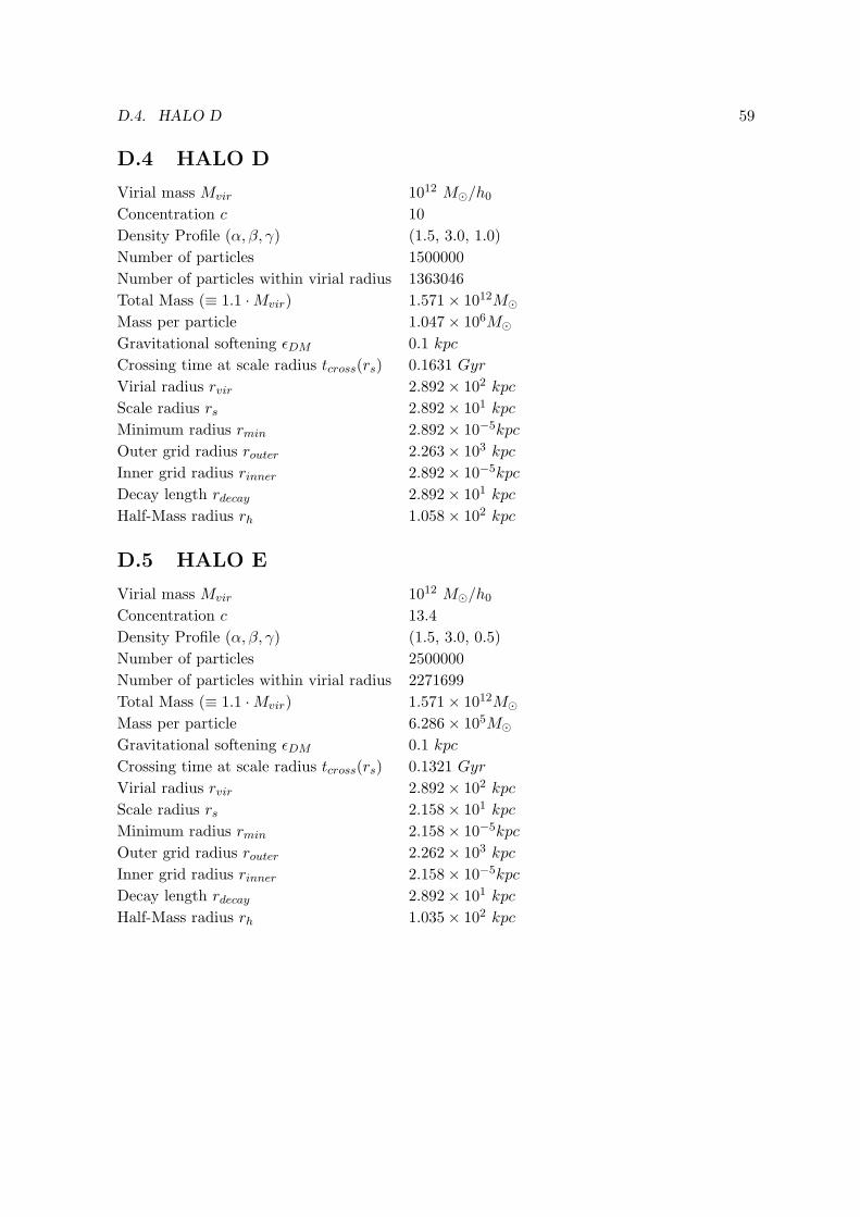
D.4. HALO D 59
D.4 HALO D
Virial mass Mvir 1012 M¯/h0
Concentration c 10Density Profile (α, β, γ) (1.5, 3.0, 1.0)Number of particles 1500000Number of particles within virial radius 1363046Total Mass (≡ 1.1 ·Mvir) 1.571× 10¹²M¯Mass per particle 1.047× 10⁶M¯Gravitational softening εDM 0.1 kpc
Crossing time at scale radius tcross(rs) 0.1631 Gyr
Virial radius rvir 2.892× 10² kpc
Scale radius rs 2.892× 101 kpc
Minimum radius rmin 2.892× 10⁻⁵kpc
Outer grid radius router 2.263× 10³ kpc
Inner grid radius rinner 2.892× 10⁻⁵kpc
Decay length rdecay 2.892× 101 kpc
Half-Mass radius rh 1.058× 10² kpc
D.5 HALO E
Virial mass Mvir 1012 M¯/h0
Concentration c 13.4Density Profile (α, β, γ) (1.5, 3.0, 0.5)Number of particles 2500000Number of particles within virial radius 2271699Total Mass (≡ 1.1 ·Mvir) 1.571× 10¹²M¯Mass per particle 6.286× 10⁵M¯Gravitational softening εDM 0.1 kpc
Crossing time at scale radius tcross(rs) 0.1321 Gyr
Virial radius rvir 2.892× 10² kpc
Scale radius rs 2.158× 101 kpc
Minimum radius rmin 2.158× 10⁻⁵kpc
Outer grid radius router 2.262× 10³ kpc
Inner grid radius rinner 2.158× 10⁻⁵kpc
Decay length rdecay 2.892× 101 kpc
Half-Mass radius rh 1.035× 10² kpc

60 APPENDIX D. DETAILED HALO SPECIFICATIONS
D.6 HALO F
Virial mass Mvir 1012 M¯/h0
Concentration c 16.2Density Profile (α, β, γ) (1.5, 3.0, 0.0)Number of particles 3000000Number of particles within virial radius 2726534Total Mass (≡ 1.1 ·Mvir) 1.571× 10¹²M¯Mass per particle 5.238× 10⁵M¯Gravitational softening εDM 0.1 kpc
Crossing time at scale radius tcross(rs) 0.1213 Gyr
Virial radius rvir 2.892× 10² kpc
Scale radius rs 1.785× 101 kpc
Minimum radius rmin 1.785× 10⁻⁵kpc
Outer grid radius router 2.261× 10³ kpc
Inner grid radius rinner 1.785× 10⁻⁵kpc
Decay length rdecay 2.892× 101 kpc
Half-Mass radius rh 1.028× 10² kpc
D.7 HALO G
Virial mass Mvir 1012 M¯/h0
Concentration c 7.5Density Profile (α, β, γ) (1.5, 3.0, 1.5)Number of particles 3000000Number of particles within virial radius 2726534Total Mass (≡ 1.1 ·Mvir) 1.571× 10¹²M¯Mass per particle 5.238× 10⁵M¯Gravitational softening εDM 0.1 kpc
Crossing time at scale radius tcross(rs) 0.2034 Gyr
Virial radius rvir 2.892× 10² kpc
Scale radius rs 3.856× 101 kpc
Minimum radius rmin 3.856× 10⁻⁵kpc
Outer grid radius router 2.264× 10³ kpc
Inner grid radius rinner 3.856× 10⁻⁵kpc
Decay length rdecay 2.892× 101 kpc
Half-Mass radius rh 1.053× 10² kpc
Core Radius rcore 2 kpc
κ 1.195× 10⁻²
Bibliography
[1] Bennett Charles et al., First Year Wilkinson Microwave Anisotropy Probe (WMAP)Observations: Preliminary Maps and Basic Results, 2003, [26]:astro-ph/0302207
[2] Binney James, Tremaine Scott, Galactic Dynamics, 1994, Princeton University Press,ISBN 0-691-08444-0
[3] Carollo Marcella, Frontiers in Astrophysics, 2003, Lecture Notes,http://www.exp-astro.phys.ethz.ch/frontiers/
[4] Cruz Fidel, Merritt David, Galactic Mergers with Supermassive Black Holes, 2001,[26]:astro-ph/0106358
[5] Eke Vincent, Cole Shaun, Frenk Carlos Cluster Evolution as a diagnostic for Ω, 1996,MNRAS, 282, 263-280
[6] El-Zant Amr, Shlosman Isaac, Dark Halos: The Flattening of the Density Cusp by dy-namical Friction, 2001, [26]:astro-ph/0103386
[7] Ferrarese Laura, Merritt David, Supermassive Black Holes, 2002, [26]:astro-ph/0206222
[8] Griest Kim, The Nature of the Dark Matter, 1996, Lectures presented at the InternationalSchool of Physics ”Enrico Fermi” Course ”Dark Matter in the Universe”, Varenna, 25July - 4 August, 1995http://web.mit.edu/∼redingtn/www/netadv/specr/012/012.html
[9] Hernquist Lars, An analytical Model for spherical Galaxies and Bulges, 1990, ApJ, 356,359-364
[10] Kazantzidis Stelios, Magorrian John, Moore Ben, Mayer Lucio, Generating equlibriumdark matter haloes, 2003, Preprint in preparation
[11] Kolb Edward, Turner Michael, The Early Universe, 1990, Addison-Wesley, ISBN 0-201-11603-0
[12] Kravtsov Andrey, Klypin Anatoly, Bullock James, Primack Joel, The Cores of DarkMatter-dominated Galaxies: Theory versus Observations, 1998, ApJ, 502, 48-58
[13] Lilly Simon, Astrophysical Cosmology, 2003, Lecture Notes,http://www.exp-astro.phys.ethz.ch/cosmology/
[14] Moore Ben, Governato Fabio, Quinn Thomas, Stadel Joachim, Lake George, Resolvingthe Structure of Cold Dark Matter Halos, 1998, ApJ, 499, L5-L8
61

62 BIBLIOGRAPHY
[15] Moore Ben, Dark matter, 1999, RSPTA, 357, 3259-3276
[16] Moore Ben, Quinn Thomas, Governato Fabio, Stadel Joachim, Lake George, Cold col-lapse and the core catastrophe, 1999, MNRAS, 310, 1147-1152
[17] Merritt David, Milosavljevic Milos, Dynamics of Dark Matter Cusps, 2002, [26]:astro-ph/0205140
[18] Merritt David, Single and binary Black Holes and their Influence on nuclear Structure,2003, [26]:astro-ph/0301257
[19] Milosavljevic Milos, Merritt David, Formation of galactic Nuclei, 2002, [26]:astro-ph/0103350
[20] Navarro Julio, Frenk Carlos, White Simon, The Structure of cold dark Matter Halos,1996, ApJ, 462, 563-575
[21] Primack Joel, The Nature of Dark Matter, 2001, [26]:astro-ph/0112255
[22] Scheck Florian, Mechanik, 1996, Springer, ISBN 3-540-61235-1
[23] Straumann Norbert, Kosmologie I, Lecture Notes
[24] Widrow Lawrence, Distribution Functions for cuspy dark Matter Density Profiles, 2000,ApJ, Supplement Series, 131, 39-46
[25] Zhao Hong Sheng, Analytical models for galactic nuclei, 1996, MNRAS, 278, 488-496
[26] Homepage of arXiv.org e-Print Archive:http://arxiv.org/
[27] Homepage of The NASA Astrophysics Data System:http://adswww.harvard.edu/