impulse measurements in earthing systems
TRANSCRIPT

- 1 -
Impulse Measurements in Earthing Systems
by
Deepak Lathi
A Thesis submitted in partial fulfillment
of the requirements for the degree of
Doctor of Philosophy
November 2012
School of Engineering
Cardiff University

- 2 -
Acknowledgements
I am very much thankful to my supervisors, Prof. A. Haddad and Dr. H. Griffiths, for
providing me an opportunity to work on this project. I am highly indebted to them, for their
valuable guidance and encouragement during the course of this project.
My special thanks are due to Megger Ltd., for sponsoring this project and providing the earth
tester and kit for use during the laboratory measurements and the field tests. I am grateful to
Mr. Graham Heritage, Mr. Daniel Hammet and Mr. Clive Pink of Megger Ltd., for the useful
discussions we had during the project progress meetings held at regular intervals.
I am highly obliged to Dr. Dongsheng Guo for his constant support during the laboratory
measurements and the field tests. The fruitful discussions which I had with him all along the
project duration helped me expedite to achieve the deliverables of the project. I am also
thankful to Dr. Noureddine Harid for his valuable support during the experiments and useful
discussions on the experimental results.
Last but not the least I would like to thank my wife Mitali, for her patience and continued
support and motivation during my studies at Cardiff.

- 3 -
Impulse Measurements in Earthing Systems
Table of Contents
Abstract .................................................................................................................................... 15
Chapter 1: Introduction ........................................................................................................ 17
Contributions of thesis ............................................................................................................. 17
1.1 Power system safety requirements ............................................................................ 18
1.2 Human Safety ............................................................................................................ 19
1.3 Functions of Earthing system .................................................................................... 20
1.4 Earthing System Safety requirements ....................................................................... 21
1.5 Recent trends in earthing impedance measurement .................................................. 23
1.6 Objectives of the project on impulse measurements in the earthing system ............. 26
1.7 Thesis Outline ........................................................................................................... 26
Chapter 2: Literature review of earthing measurement techniques ..................................... 29
2.1 Introduction ............................................................................................................... 29
2.2 Methods of measurement of earth impedance ........................................................... 30
2.2.1 Fall of potential method ..................................................................................... 31
2.2.2 Two-point method .............................................................................................. 34
2.2.3 Three point method ............................................................................................ 35
2.2.4 Ratio method ...................................................................................................... 36
2.2.5 Staged fault test .................................................................................................. 36
2.2.6 Single clamp earth resistance testing method .................................................... 36
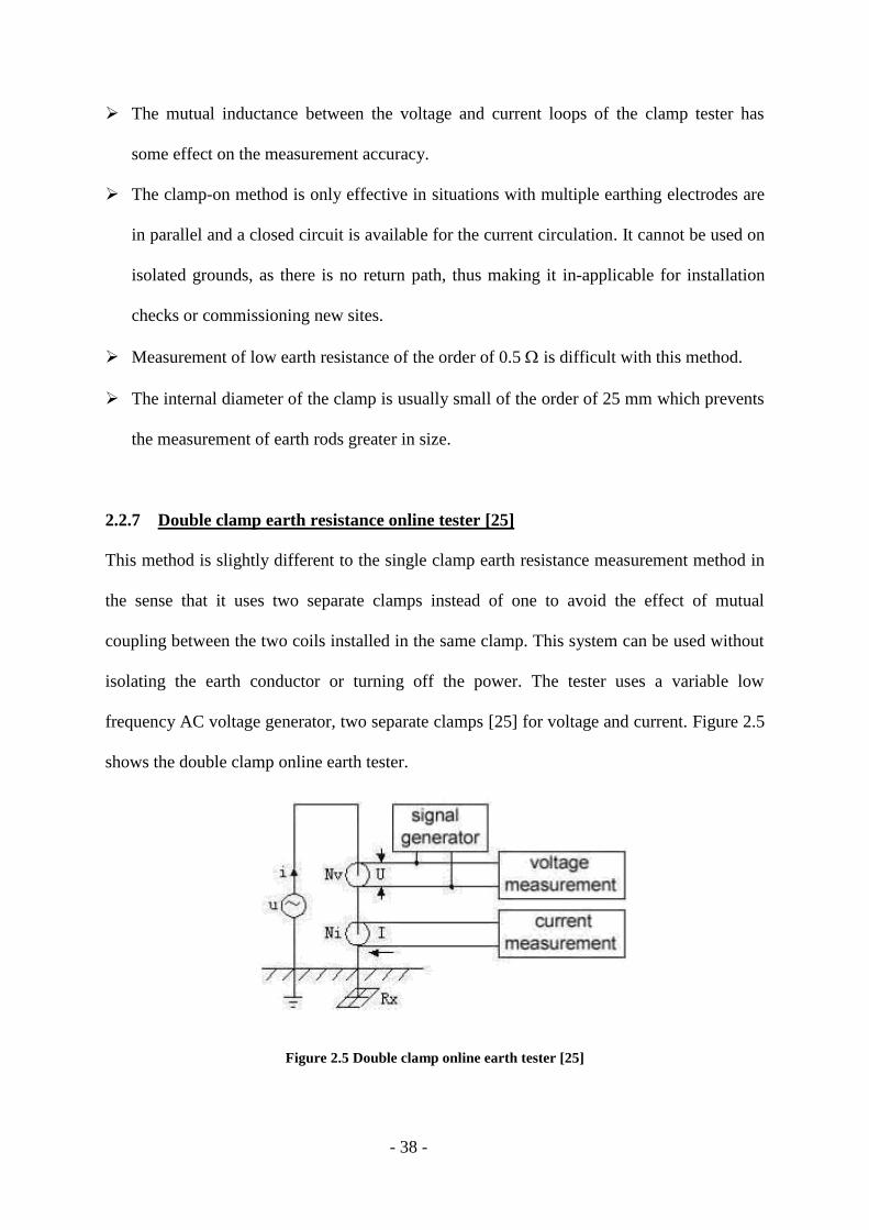
2.2.7 Double clamp earth resistance online tester [25] ............................................... 38
2.2.8 Attached rod technique (ART) by Megger [24] ................................................ 40
2.3 Comparative study of earth testers ............................................................................ 41
2.3.1. Commercially available earth testers ................................................................. 41

- 4 -
2.4 Smart ground meter [27] ........................................................................................... 44
2.5 Effect of pin spacing on the measured earth impedance ........................................... 49
2.6 Conclusion ................................................................................................................. 52
Chapter 3: Determination of accuracy of transducers and preliminary laboratory tests ..... 54
3.1. Introduction ............................................................................................................... 54
3.2. Voltage transducers ................................................................................................... 54
3.3. Current transducers ................................................................................................... 57
3.4. Laboratory tests of earth resistance meters and earth impedance measurement
system (IMS) ........................................................................................................................ 59
3.4.1. DET 2/2 laboratory tests .................................................................................... 59
3.4.1. IMS laboratory tests ........................................................................................... 60
3.4.2. ABEM Terrameter laboratory tests .................................................................... 61
3.1 Laboratory tests of impedance measurements of soil and electrolytes ..................... 62
3.2 Conclusion ................................................................................................................. 76
Chapter 4: Description of test sites and facilities ................................................................ 78
4.1. Overview of Llanrumney fields test site ................................................................... 78
4.2. Overview of Dinorwig test site ................................................................................. 82
4.2.1. Water resistivity measurements ......................................................................... 83
4.2.2. Resistivity measurement survey on 09/05/2007 ................................................ 84
4.2.3. Resistivity measurement survey on 19/07/2007 ................................................ 85
4.2.4. Resistivity measurement survey on 01/08/2007 ................................................ 87
4.3. Experimental set up at Dinorwig Test Site................................................................ 88
4.4. Description of earthing impedance measurement (IMS and Impulse) systems ........ 92
4.4.1. Cardiff University Impedance Measurement System (IMS) ............................. 92
4.4.2. Radio Frequency System (RF) ........................................................................... 95
- 5 -
4.4.3. Impulse current injection system ....................................................................... 95
4.5. Measurement of resistivity at test site locations with ABEM Terramer ................... 95
4.5.1. Measurement of Resistivity at Llanrumney fields ............................................. 95
4.5.2. Measurement of Resistivity at Dinorwig ......................................................... 100
4.6. Summary ................................................................................................................. 104
Chapter 5: Characterisation of earth electrodes under variable frequency and impulse
energisation using full scale field tests .................................................................................. 106
5.1. Tests on single earth rod at Llanrumney test site .................................................... 107
5.1.1. Earth resistance / impedance tests on single earth rod ..................................... 107
5.1.2. Low Voltage Impulse Tests on Single Earth Rod ............................................ 111
5.2. Tests on single earth rod at Dinorwig test site ........................................................ 114
5.2.1. Rod ‘earth’ impedance ..................................................................................... 117
5.2.2. Variable frequency earth impedance measurement ......................................... 117
5.2.3. Low voltage impulse tests ................................................................................ 120
5.2.4. Effect of current magnitude on measured earth impedance of signle rod at
Dinorwig ........................................................................................................................ 121
5.3. Tests on 3m x 3m grid at Llanrumney test site ....................................................... 123
5.4. Tests on 5m x 5m grid at Dinorwig test site ........................................................... 126
5.4.1 Tests on the electrode Grid 1 ........................................................................... 126
5.4.2 DC earth resistance of Grid 1........................................................................... 127
5.4.3 Current magnitude dependence of the impedance of Grid 1 ........................... 127
5.4.4 Low voltage impulse tests on Grid 1 ............................................................... 127
5.4.5 Tests on the electrode Grid 2 ........................................................................... 127
5.5. Tests on the horizontal electrode ............................................................................. 131
5.5.1 DC earth resistance of Horizontal Electrode 2 ................................................ 132

- 6 -
5.5.2 The current magnitude dependence of impedance of Horizontal Electrode 2 . 132
5.6. Tower base tests at Llanrumney .............................................................................. 133
5.6.1. Purpose built test Tower base (TTB) ............................................................... 133
5.6.2. Operational tower (VP9) tests .......................................................................... 136
5.7. Large area earthing system at Llanrumney ............................................................. 137
5.7.1 Ring Earthing System connected with Test Tower Base ................................. 137
5.7.2 Cluster of Three Rods connected with Horizontal Electrode at Llanrumney .. 139
5.7.3 Cluster of Three Rods at Llanrumney .............................................................. 140
5.8. Discussion of test results ......................................................................................... 141
5.8.1 Comparison of FFT from impulse and swept frequency results ...................... 141
5.8.2 Frequency dependence of earth electrode impedance ..................................... 144
5.8.3 Dependence of earth electrode impedance on injected current magnitude ...... 145
5.8.4 Impulse response of earth electrode impedance .............................................. 145
5.9. Conclusion ............................................................................................................... 145
Chapter 6: Comparison of experimental results with simulation ...................................... 147
6.1. Computer modelling ................................................................................................ 147
6.1.1 Concentrated earthing systems ........................................................................ 147
6.1.2 Cluster of rods of the ring earthing system at Llanrumney ............................. 154
6.1.3 Operational 275kV tower base (VP9) .............................................................. 155
6.1.4 Comparison of simulation with experimental test results (Dinorwig test site) 158
6.2. Conclusion ............................................................................................................... 162
Chapter 7: Analysis of current and frequency effects on earth resistance and earth
impedance 163
7.1. Introduction ............................................................................................................. 163
7.2. Soil conduction review ............................................................................................ 163

- 7 -
7.3. Analysis of measured effect of frequency on impedance of earth electrode .......... 164
7.4. Frequency dependence of clay water electrolyte properties: an overview .............. 166
7.5. Effect of current on the measured earth impedance ................................................ 169
7.6. Nonlinear current effect .......................................................................................... 171
7.7. Comparison of variation of normalized impedance with current density ............... 176
7.8. Conclusion ............................................................................................................... 177
Chapter 8: Conclusion and Future Scope of Work ............................................................ 179
8.1. Advantages and limitations of different earthing measurement techniques ........... 179
i) Switched DC Technique: ....................................................................................... 180
ii) Variable frequency AC Technique:........................................................................ 180
iii) FFT from impulse and calculating the impulse resistance from the waveforms: .. 181
8.2. Validity range of earthing measurement techniques ............................................... 182
8.3. Feasible current and frequency ranges for earth impedance measurement ............. 183
8.4. Future scope of work ............................................................................................... 185
References .............................................................................................................................. 187
Appendix A1 .......................................................................................................................... 195
A1.1 Specifications of the voltage transducers ............................................................ 195
A1.2 Specifications of the current transducers ............................................................. 196
A1.2.1 LILCO BROADBAND CURRENT TRANSFORMER ................................ 196
A1.2.2 Stangenes Pulse Current Transformer ............................................................ 199
- 8 -
List of Figures
Figure 2.1 Typical set up of fall of potential test ..................................................................... 32
Figure 2.2 Fall of potential profiles ......................................................................................... 33
Figure 2.3 Two-point method [11] ........................................................................................... 34
Figure 2.4 Clamp on earth resistance testing .......................................................................... 37
Figure 2.5 Double clamp online earth tester [25] .................................................................... 38
Figure 2.6 Attached rod technique (ART) measurement (Megger) [24] ................................ 40
Figure 2.7 Sample waveform of the pseudorandom signal [27] .............................................. 45
Figure 2.8 Smart Ground Meter [27] ....................................................................................... 46
Figure 2.9 Measurement set up for smart earth meter [27] ...................................................... 46
Figure 2.10 Percentage error in computed grid resistance as a function of pin spacing [63] .. 51
Figure 3.1 Test setup for calibration of differential probes ..................................................... 55
Figure 3.2 Determination of the accuracy of the voltage transducer SI 9000 serial number
26950........................................................................................................................................ 56
Figure 3.3 Determination of the accuracy of the voltage transducer DP25 serial number
20080843.................................................................................................................................. 56
Figure 3.4 Test set up for comparison of current transducers .................................................. 57
Figure 3.5 Comparison of current transducers ......................................................................... 58
Figure 3.6 Measurement of Cropico MTS1A standard 1Ω resistance with DET 2/2 ............. 59
Figure 3.7 Measurement of Cropico MTS1A standard 1.9Ω resistance with DET 2/2 .......... 60
Figure 3.8 Measurement of Cropico MTS1A standard 10Ω resistance with DET 2/2 ........... 60
Figure 3.9 Measurement of resistance with Cardiff University Impedance Measurement
System ...................................................................................................................................... 61
Figure 3.10 Measurement of resistance with ABEM Terrameter ............................................ 61
Figure 3.11 Test set-up for laboratory tests on the soil and water. .......................................... 62

- 9 -
Figure 3.12 Effect of frequency on the impedance of 3.24% wet sand filled in the test cell . 63
Figure 3.13 Effect of frequency on the impedance of dry sand filled in the test cell ............. 64
Figure 3.14 Effect of frequency on the impedance of tap water filled in the test cell ............ 65
Figure 3.15 Effect of frequency on the impedance of distilled water filled in the test cell .... 66
Figure 3.16 Effect of frequency on the impedances of various conducting mediums filled in
the test cell ............................................................................................................................... 67
Figure 3.17 Effect of current magnitude on the impedance of 3.24% wet sand filled in the
test cell ..................................................................................................................................... 68
Figure 3.18 Effect of current magnitude on the impedance of tap water filled in the test cell
.................................................................................................................................................. 69
Figure 3.19 Effect of current magnitude on the impedance of dry sand filled in the test cell 70
Figure 3.20 Effect of current magnitude on the impedance of distilled water filled in the test
cell ............................................................................................................................................ 71
Figure 3.21 Effect of DC current magnitude on the impedance of different current mediums
filled in the test cell .................................................................................................................. 72
Figure 3.22 Effect of AC current magnitude on the impedance of different current mediums
filled in the test cell .................................................................................................................. 72
Figure 3.23 Variation of impedance of water with frequency ................................................. 73
Figure 3.24 Variation of resistivity of water with frequency ................................................... 74
Figure 3.25 Percentage change in resistivity of water with frequency from 20Hz to 120kHz
with increasing electrolyte concentration ................................................................................ 75
Figure 4.1 Plan view of University test site at Llanrumney showing outline of installed test
electrodes ................................................................................................................................. 79
Figure 4.2 Tower footing construction of one leg of tower base ............................................. 80
Figure 4.3 Plan view of the four legs of the Tower base ......................................................... 80

- 10 -
Figure 4.4 Isometric view of 3m x 3m grid ............................................................................. 81
Figure 4.5 Plan view of ring earthing system .......................................................................... 81
Figure 4.6 Plan of the lower reservoir at Dinorwig power station showing water resistivity
test locations............................................................................................................................. 83
Figure 4.7 Water resistivity and conductivity measurement results on 19/07/2007 ................ 86
Figure 4.8 Side view of the test set up at Dinorwig ................................................................. 89
Figure 4.9 Plan view of test set up 1 (injection source placed in the test cabin 150m away
from the test object) ................................................................................................................. 89
Figure 4.10 Plan view of test set up 1 (injection source placed near the test object) .............. 91
Figure 4.11 View of 5m x 5m grid installed at the far end of the pontoon chain .................... 92
Figure 4.12 Principle of operation of lock-in amplifier ........................................................... 93
Figure 4.13 Impedance Measurement System ......................................................................... 94
Figure 4.14 Electrodes spacing in Wenner configuration ........................................................ 97
Figure 4.15 Gradient array layout showing the position of electrodes for a measurement of
Wenner configuration with s factor of 8 and n factor of 2. ...................................................... 97
Figure 4.16 Soil resistivity survey lines at Llanrumney .......................................................... 97
Figure 4.17 Soil resistivity survey performed on 23rd
January 2009 ....................................... 98
Figure 4.18 Soil resistivity survey performed on 1st April 2009 ............................................. 99
Figure 4.19 Measured apparent resistivity against Wenner spacing...................................... 101
Figure 4.20 Two dimension resistivity distributions ............................................................. 103
Figure 4.21 Resistivity of lake bed in two measurements ..................................................... 104
Figure 5.1 Test set-up for measurement of earth impedance of single earth rod ................... 108
Figure 5.2 Earth impedance tests with IMS on a single 2.4m earth rod ................................ 110
Figure 5.3 Variation of impedance with current ................................................................... 111
Figure 5.4 Low voltage impulse (LVI1) test waveforms ....................................................... 112

- 11 -
Figure 5.5 Low voltage impulse (LVI2_B) test waveforms .................................................. 113
Figure 5.6 Comparison of FFT of impulse waveforms and frequency scan of earth
impedance for single rod ........................................................................................................ 113
Figure 5.7 Plan view of test set up for testing single rod at Dinorwig test site ..................... 114
Figure 5.8 Effect of current magnitude on measured earth resistance ................................... 116
Figure 5.9 Plots of measured and simulated earth impedance magnitude with frequency .... 119
Figure 5.10 Lumped parameter circuit model for a rod electrode ......................................... 120
Figure 5.11 Low voltage impulse test results on a 0.8m rod ................................................. 121
Figure 5.12 Effect of current magnitude on earth impedance of single rod at Dinorwig test
site .......................................................................................................................................... 122
Figure 5.13 Effect of frequency on earth impedance of single rod at Dinorwig test site ...... 122
Figure 5.14 Experimental setup for tests on 3m x3m grid at Llanrumney test site ............... 123
Figure 5.15 Effect of current on earth impedance of 3m x 3m grid ...................................... 124
Figure 5.16 Impulse waveforms ............................................................................................ 125
Figure 5.17 Variation of impedance with frequency scan and that computed from the FFT of
impulse ................................................................................................................................... 126
Figure 5.18 Plan view of test set up for testing 5m x 5m earth grid and horizontal electrode at
Dinorwig ................................................................................................................................ 128
Figure 5.19 Current dependence of earth impedance of a Grid 1 at 20Hz and 52Hz ............ 129
Figure 5.20 Current dependence of earth impedance of a Grid 1 at DC current (ABEM) .... 129
Figure 5.21 Effect of frequency on earth impedance of 5m x 5m grid at Dinorwig test site 130
Figure 5.22 Comparison of Swept frequency and FFT from impulse methods of measurement
of earth impedance of 5m x 5m earth grid. ............................................................................ 130
Figure 5.23 Effect of frequency on earth impedance of horizontal electrode at Dinorwig test
site .......................................................................................................................................... 131

- 12 -
Figure 5.24 Current magnitude dependence of earth impedance of a horizontal electrode .. 133
Figure 5.25 Set up for measuring earth impedance of test tower base at Llanrumney .......... 134
Figure 5.26 Effect of frequency on tower earth impedance tested at Llarumney .................. 135
Figure 5.27 Effect of current on tower earth impedance tested at Llanrumeny .................... 135
Figure 5.28 Comparison of effect of frequency on earth impedance of tower base tested at
Llanrumney ............................................................................................................................ 137
Figure 5.29 Effect of frequency on large area earthing system at Llanrumney ..................... 138
Figure 5.30 Test set up for Cluster of Three Rods with Horizontal Electrode ...................... 139
Figure 5.31 Variation of impedance with frequency (Cluster of Three Rods with Horizontal
Electrode) ............................................................................................................................... 139
Figure 5.32 Plan view of test set up (Cluster of Three Rods) ................................................ 140
Figure 5.33 Variation of impedance with frequency (3 rod cluster)...................................... 140
Figure 5.34 FFT of slow impulse waveform with different windowing functions ................ 142
Figure 5.35 FFT of fast impulse waveform with different windowing functions (enlarged
view) ...................................................................................................................................... 142
Figure 5.36 Comparison of measured earth impedance obtained from frequency scan with the
earth impedance computed from FFT of measured impulse signals ..................................... 143
Figure 5.37 Comparison of AC steady state measurements with impulse ............................ 144
Figure 6.1 Isometric view of 3m x 3m grid ........................................................................... 148
Figure 6.2 Tower footing construction of one leg of tower base ........................................... 149
Figure 6.3 Plan view of the four legs of the Tower base ....................................................... 150
Figure 6.4 Comparison of simulated and measured earth impedance of single rod .............. 150
Figure 6.5 Comparison of simulated and measured earth impedance of 3mx3m grid .......... 151
Figure 6.6 Comparison of simulated and measured earth impedance of test tower base ...... 151
Figure 6.7 Comparison of simulated and measured earth impedance of cluster of rods ....... 155

- 13 -
Figure 6.8 Comparison of simulated and measured earth impedance of cluster of rods ....... 155
Figure 6.9 Comparison of simulated and measured earth impedance of operational 275kV
tower base VP9 with overhead earth wire connected ............................................................ 157
Figure 6.10 Comparison of simulated and measured earth impedance of operational 275kV
tower base VP9 with overhead earth wire dis-connected ...................................................... 158
Figure 6.11 Comparison of simulated and measured earth impedance of Rod 2A ............... 160
Figure 6.12 Comparison of simulated and measured earth impedance of Grid 1 .................. 160
Figure 6.13 Comparison of simulated and measured earth impedance of Grid 2 .................. 161
Figure 6.14 Comparison of simulated and measured earth impedance of single rod at
Dinorwig ................................................................................................................................ 161
Figure 7.1 Model of conduction of electric current through soil micro-pores reproduced from
[44] ......................................................................................................................................... 164
Figure 7.2 Effect of frequency on earth impedance for various electrodes ........................... 165
Figure 7.3 Normalized effect of frequency on earth impedance ........................................... 165
Figure 7.4 Conductivity dispersion in soil sample [46] ......................................................... 167
Figure 7.5 Effect of current on earth impedance ................................................................... 170
Figure 7.6 Normalized effect of current on earth impedance ................................................ 171
Figure 7.7 Current dependence of electrode electrolyte interface observed by Ragheb and
Geddes.................................................................................................................................... 174
Figure 7.8 Frequency response and current dependence of the electrode-electrolyte interface
resistance observed by Ragheb and Geddes [62] ................................................................... 175
Figure 7.9 Polarization effect observed during field tests (Effect is pronounced at lower
frequencies ~20Hz to 100Hz) ................................................................................................ 175
Figure 7.10 Comparison of normalized effect of current density on earth impedance .......... 177

- 14 -
List of Tables
Table 2.1 Summary of the comparison of the commercially available earth testers ............... 41
Table 2.2 Summary of comparison of commercially available earth testers ........................... 43
Table 2.3 Computed grid resistance error range ...................................................................... 51
Table 3.1 Groups of current transducers formed for testing purpose ...................................... 57
Table 4.1 Typical water resistivity measurement results on 09/05/2007................................. 85
Table 4.2 Water resistivity measurement results on 01/08/2007 ............................................. 87
Table 4.3 List of earth electrodes tested at Dinorwig test site ................................................. 92
Table 4.4 Two layer soil model used for simulation ............................................................. 100
Table 4.5 Resistivity model of Dinorwig test site.................................................................. 102
Table 5.1 Comparison of measured earth resistance / impedance with analytical impedance
................................................................................................................................................ 117
Table 5.2 Parameters of the impulse waveforms ................................................................... 121
Table 6.1 Two layer soil model of Llanrumney test site used for simulation ...................... 147
Table 6.2 Seasonal variation in the measured earth impedance ............................................ 153
Table 6.3 Two layer soil model of operational 275kV tower base at Llanrumney test site . 156
Table 6.4 Resistivity model of Dinorwig test site.................................................................. 158
Table 6.5 List of earth electrodes tested at Dinorwig test site ............................................... 159
Table 7.1 Values of constants for different electrode metals tested ...................................... 172
Table 7.2 Calculated values of polarization impedance ........................................................ 174
Table A1.1 Technical specifications of SI 9000 .................................................................... 195
Table A1.2 Technical specifications of DP25 ....................................................................... 196

- 15 -
Abstract
The behaviour of earth electrodes at power frequency conditions is well known. Several
studies are going on at present, to understand the behaviour of earthing systems at transient
impulse and high frequency conditions. The study of impulse measurements in earthing
systems was carried out during this project, to understand the soil electromagnetic behaviour
towards high frequency and variable AC/DC/impulse current magnitudes. Several
measurement techniques and instrumentation used for the measurement of the earthing
systems were surveyed. The limitations and the advantages of each approach have been
identified, and the range of application determined. Extensive experiments were performed
on the practical earth electrodes at the Cardiff University test site at Llanrumney, and at the
Dinorwig power station earthing facilities. These experiments have revealed that there is
reduction of impedance of earth electrodes over the frequency range 20Hz to 120kHz.
Moreover, a pronounced effect of DC current magnitude was observed on the earth resistance
of the electrodes over the range of 1mA to 500mA. The numerical modelling of the test
configurations did not show the reduction in earth impedance over the frequency range 20Hz
to 120kHz. To understand the different trends shown by the experiments and simulation, and
the effect of frequency and current magnitude, a geological literature survey was carried out.
This survey revealed that when the soil water electrolyte solution is subjected to high
frequency electrical currents, it exhibits conductivity dispersion phenomenon. Conductivity
dispersion is a phenomenon where conductivity of the clay water electrolyte solution
increases by about 30% over a frequency range 20Hz to 100kHz. The geological literature
survey also revealed that the polarisation effect in the soil water electrolyte is responsible for
the non-linear current effect.
Moreover, during this project, a new technique of FFT from impulse, was proposed to
measure the earth electrode impedance, over a frequency range which is an inherent

- 16 -
component of the impulse signals. The FFT from impulse signals, showed a good agreement
of the measured earth impedance of the earth electrodes, with the measured earth impedance
using the variable frequency scan method. FFT from impulse technique has an advantage
over the variable frequency scan method, from the point of view of the time required for the
measurement and the simplicity of the test source, for the measurement of the earth electrode
impedance. Such a technique, could have impact on the testing at high current magnitudes,
where impulse generation is much easier. Finally, the future scope of work is presented to
explore the measurement of earth electrode impedance above the frequency of 120kHz and
current magnitudes above 5A.

- 17 -
Chapter 1: Introduction
Contributions of thesis
1. Surveyed the measurement techniques and instrumentation used for earthing systems
measurements. The limitations and advantages of each approach have been identified and
the range of application determined.
2. Variable frequency AC, DC and impulse tests have been conducted on several full scale
earth electrodes at the University earthing test site at Llanrumney and the Dinorwig
power station earthing test facility.
3. The extensive experimental data has been analysed and compared with numerical
modelling of the test electrode configurations.
4. In particular, the measured earthing impedances of various electrodes were found to be
frequency dependent, over the range 20Hz to 120kHz. The impedances of the practical
earth electrodes reduced up to 30% when the frequency of injected current was increase
from 20Hz to 120kHz. The effect of frequency was attributed to the conductivity
dispersion phenomenon revealed by the geological literature survey. Furthermore, the
measured earth electrode impedances were also found to be AC / DC current dependent
for injected current magnitudes below 100mA, with a pronounced effect for DC currents.
The current dependence was attributed to soil polarisation phenomena observed in the
geological literature survey.
5. A new FFT analysis of impulse test data was proposed and applied in this work. Good
agreement was obtained between the frequency dependence determined by the FFT
approach and the results from the direct injection of variable frequency current. Such
approach could have important significance for testing of high current magnitudes, where
impulse generation is much easier.

- 18 -
1.1 Power system safety requirements
The demand for electrical power has been rising due to rapid economic development in the
last century. In order to meet this increased demand, the size and capacity of power stations
and substations continue to increase. This growth in capacity and greater interconnection has
led to a continued increase in fault current levels. It is desired to have zero tolerance
protection system for compact gas insulated substations which are characterised by fast
transients and proximity to the public utilities. The tall wind power installations are prone to
lightning strikes. The interconnected high and medium voltage power systems require
limitation of the step, touch and transferred earth potentials to the permissible values. The
high voltage transmission systems close to the public access areas demand heightened safety
of equipment and personnel. The proximity of high voltage transmission systems to
communication circuits demands very high reliability of power system protection. It is also
important to limit the back flashover voltages during direct lightning strike. One of the key
factors to provide the heightened safety and reliable means of protection lies in the efficient
design and maintenance of low impedance earthing systems. The role of electrical earthing
systems is also crucial in maintaining the continuity of service of the power supply. In the
event of fault, the resulting high-magnitude currents have to be interrupted as fast as possible
in order to protect the electrical equipment and personnel working in the vicinity. These
conditions necessitate an efficient earthing system which helps with effective and fast
discrimination of the fault currents from the load currents. Efficient earthing systems in co-
ordination with the protective relays also help in discriminating the locations of the faulty
zones and thereby isolating them effectively before the fault spreads to a wider area. The
advanced electronic equipment installed for protection and control purpose in the modern
power installations are susceptible to the dangers due to the rise of earth potential [1].
Effective earthing systems keep the rise of earth potential within safety limits. The

- 19 -
telecommunications circuits running adjacent to the power lines may get subjected to earth
potential rise due to transferred earth potentials and thereby get damaged. If the earthing
impedance is low, the earthing system will be able to absorb high currents without the earth
potential rising to dangerously high levels during lightning strikes. If the earthing impedance
is high, the lightning strike can cause back flashover directly involving a phase conductor. To
obtain safety from direct lightning strikes, an essential aspect is to adopt adequate earthing
system, with the eventual need for additional measures such as shielding and overvoltage
limiting equipment. It is important to limit the current amplitude of lightning strikes incident
in protected zones to be carried by the power circuits by appropriately diverting it to the
earthing circuits. However, in the case of power system short circuit faults, the currents are
inherently originating from the power circuits which will have to be interrupted by the
protective relays in the shortest possible time period. Low impedance earthing systems help
with faster determination of the fault currents by the protective relays which operate on the
combination of sensing the rate of change of current with time and absolute magnitude of the
fault current. The magnitude of earth impedance is an important performance indicator of the
earthing system.
1.2 Human Safety
The tolerance of human beings subjected to shock scenarios depends on the amount of
current passing through the human body, which in turn depends on the earth potential rise.
Dalziel et al. [2, 3] and Beigelmeier et al. [4] suggested that the electric currents below 5mA
can be safely conducted by human body. Electric currents above 5mA can cause effects on
the human body depending on the individual weight, duration of exposure and magnitude of
the current. However, electric currents above 200mA to 300mA for more than 1 second
duration [4] can be severely harmful to human beings as it causes ventricular fibrillation

- 20 -
(heart muscles resulting in interference with rhythmic contractions of the ventricles and
possibly leading to cardiac arrest).
1.3 Functions of Earthing system
Earthing systems are required to manage the transfer of fault energy in such a manner as to limit
the risk to people, equipment and system operation to acceptable levels. An earthing system is
required to perform this function for the life of the electrical network for which it is installed, for
the range of configurations of the network and nearby infrastructure that are foreseeable. The
earthing system may need to be augmented over time so as to continue to fulfil this function. The
earthing system is required to limit the level of transient voltage and power frequency voltage
impressed on electrical equipment. It is also required to provide appropriate current paths for fault
energy in such a manner that those fault energies do not impair equipment or equipment
operation. System events/disturbances may otherwise cause extensive damage to equipment and
associated ancillary equipment such as insulation breakdown and thermal or mechanical damage
from arcing, fires or explosions. The earthing system is required to ensure proper operation of
protective devices such as protection relays and surge arresters to maintain system reliability
within acceptable limits. It is intended to provide a potential reference for these devices and to
limit the potential difference across these devices. The earthing system is required to achieve the
desired level of system reliability through facilitating the proper and reliable operation of
protection systems during earth faults. This entails reliable detection of earth faults and either
clearing the fault or minimising the resulting fault current. In order to meet the foregoing
operational requirements earthing systems need to be adequately robust and able to be monitored.
Robustness - The earthing system, its components and earthing conductors shall be capable of
conducting the expected fault current or portion of the fault current which may be applicable and
without exceeding material or equipment limitations for thermal and mechanical stresses.

- 21 -
Ongoing monitoring – The earthing system shall be designed and configured to enable the system
to be tested at the time of commissioning and at regular intervals as required, and to enable cost
effective monitoring of the key performance parameters and/or critical items.
1.4 Earthing System Safety requirements
The safe earthing system is expected to meet the following objectives,
a) Provide means to carry electric currents into the earth under normal operating conditions,
fault conditions, switching transients and lightning strike without the rise of earth potential
exceeding the safe limits and to maintain continuity of the service [5].
b) Provide safety of the operating personnel in the vicinity of the earthing system by limiting
the amplitude of the step, touch and transferred earth potentials during power system fault
conditions and transient phenomenon such as lightning.
A transmission line surge arrester conducts a lightning surge to a low impedance earthing
systems to protect the surrounding insulators from the excessive flashover voltages which
would have otherwise developed. It is desired that the earthing system provides least
impedance path to the flow of lightning impulse currents, transient surge fault currents and
power frequency fault currents to limit the rise of earth surface potentials within the
permissible values. It is, therefore, required to study the behaviour of the earthing systems
under these different conditions to predict its effectiveness. The impedance of an earthing
system depends on various factors such as the soil resistivity and permittivity of the general
mass of the earth carrying the surge currents, the geometry of the earthing electrode and the
magnitude and wave front rise time of the current surge. The aging of earthing conductor
system as a result of corrosive action of the soil also affects the impedance of earthing
system. These aspects pose many challenges in designing an effective earthing system such
as to cope with the seasonal changes in the resistivity of soil and the aging effects due to

- 22 -
corrosion properties of various soil will have to be adequately predicted during the design
phase. In addition to verifying the design of earthing systems at new stations to meet the
requirements, the adequacy of the earthing system performance at existing stations, especially
at the very old stations where the earthing grid design is unknown, has to be monitored
periodically to ascertain its efficiency.
Lightning protection of transmission lines has attracted a lot of attention of electrical
engineers in the past. Initial efforts were in the direction of reducing the induced voltages due
to lightning strike on the transmission lines. But later on, it was observed that it was the direct
lightning strike which resulted in outages of high voltage power transmission circuits. Efforts
were then made to shield the overhead open wires with an earth wire running on the top of
the transmission towers. Lightning earths are expected to have least possible impedance to
high frequency currents. Lightning surge characteristics of an earthing system have an
influence on electromagnetic transient behaviours in low-voltage and control circuits. The
lightning surge phenomena are important factors for determining the insulation level of the
power transmission equipment. Hideki Motoyama [12] conducted experiments on earth mesh
to evaluate the lightning surge characteristics by analysis of transient potential rise at various
points in the earth mesh. The theoretical analysis of lightning surge characteristics by Sunde
[13] is well known. The soil resistivity and the electric permittivity ε are frequency
dependant [14]. The magnetic permeability is in general equal to permeability of free space
0. Power transmission line earthing systems are usually assumed as extended earthing
systems. Leonid Grcev [15] observed that the propagation effects are dominant in early time
in the extended earthing systems, when the earthing systems are subjected to fast front
lightning currents. He analysed the dynamic behaviour of such earthing systems taking into
consideration the propagation effects. The wavelength of the electromagnetic wave in the soil
depends on the soil resistivity. Therefore, the classification of the earthing systems as

- 23 -
concentrated or extended may be quite different in different soils for a particular current
impulse.
The first strike of a lightning surge is characterised by the frequency components in the range
of few tens of kHz to few hundreds of kHz. Similar-frequency currents exist in switching
transients. The frequencies of the order of few MHz are present in the subsequent return
strokes of a lightning surge. These phenomena were the motivation behind studying the
behaviour of the earthing systems over a high frequency range. Most of the commercial earth
resistance testers measure earthing resistance by injecting switched DC signals into the earth
electrode. This resistance is an estimate for predicting the behaviour of the earthing system
under power frequency conditions. However, the behaviour of earthing systems during
lightning strike or transient faults is considerably different from that at power frequency and
low currents.
1.5 Recent trends in earthing impedance measurement
Conventional instruments generally inject switched DC signals at low frequency (typically
128 Hz) to measure the resistance of the earthing system. However, in case of the large
earthing systems, the DC resistance is quite low while the inductive reactance is generally
higher in magnitude, so it becomes relevant to measure the impedance of the earthing system.
The measurement of impedance of the large earthing system requires injection of the AC
currents at the frequencies close to the power frequencies. On the other hand, if a spectrum of
transient surges and lightning surges is observed, then it reveals various components of low
and high frequencies. High frequency components are a result of the fast rising wave fronts
and the low frequency components are contributed by the wave tail of the surges. In order for
the earthing system to be effective, it should be able to control the earth potential rise during
the absorption of the power frequency fault currents as well as transient frequency surges.

- 24 -
The impulse behaviour of the wire-type electrodes, buried horizontally, differ quite markedly
depending on whether or not electrode length is negligible, in comparison with wavelength of
transient phenomena. The distinction between the concentrated and extended electrodes is
based on the importance of the inductance terms compared with the resistance terms.
Therefore, besides considering the maximum slope of the impulse current front, it is
necessary to consider soil resistivity too, because if the soil resistivity is high, it results in
increase in resistive drop in relation to the inductive drop. Mazetti et al. [41] presented a
mathematical model to analyse the transient behaviour of buried earth wire when fed at one
side by an impulse current similar to a lightning stroke. In case of a lightning strike, the
earthing has to absorb the lightning energy in a very short duration [30]. Considering that the
flow of current (electrons) is at the speed of light, a 0.2 s rise time (wave front) of lightning
restrike phenomenon will result in the length of lightning current flow up to 30 meters (speed
of light x rise time) by the time wave front is over. So, a 30 meter rule is being used in the
Lightning earthing systems, which shows that the effective length of a lightning earthing
system is up to 30 meters, indicating that the earthing system beyond this point will not play
any role in absorbing the energy of a lightning restrike. Injecting various frequency current
waveforms in the earthing system and analysing the response of earthing to these waveforms
provides an order of magnitude impedance of the earthing system over a range of various
frequencies. Previous studies [6, 7] have indicated that the behaviour of earthing systems
excited by lightning impulse and phase to earth faults considerably differ from that of low
frequency injection. Jong-kee et al. [33] experimentally measured the earth impedance of
mesh type earth grid in the frequency range from 0.1 Hz to several hundred kHz. The
published studies of the transient behaviour of earth electrodes of various forms (horizontal
wires, vertical rods and mesh networks) from the theoretical [34-37] or experimental [38-40]
point of view helped in improving the knowledge of performance of earthing systems in

- 25 -
lightning conditions. Leonid Grcev and Markus Heimbach [6] did transient analysis of large
earthing systems to study the influence of soil resistivity, location of feed point, grid size,
depth, conductor separation, earth rods and shape of the lightning current impulse, on the
transient performance of earth grids of different sizes.
Rong Zeng et al. [8] developed a new method of measuring earth impedance. According to
the theoretical analysis carried out by them, it is proposed that there lies a fixed voltage
electrode position between the earth electrode and current electrode position in fall of
potential method irrespective of the length of the current electrode from the earth electrode.
Based on this analysis they proposed to calculate this position which they named as a
compensating position of the potential electrode with the help of a computer programme.
Following inputs are required for their programme such as soil resistivity data of various
locations in the vicinity of earthing system, earthing system topology, length of current
electrode from the earth electrode. The resulting potential distribution profile gives guidance
on where the potential probe should be placed, so as to get the value of the true earth
resistance. Griffiths et al. [32] used the Lock-in amplifier technique to inject variable
frequency signal in the earthing system under test. From the experiments, they found out that
injecting the frequencies of 48 Hz and 52 Hz gives the least effect of background noise at a
power frequency of 50 Hz. They successfully tested the earthing impedance measurement
system based on lock in amplifiers on different substations and transmission environments.
Rong Zeng et al. [8] used the swept frequency method to measure the impedance of earthing
systems. In their system, the effect of noise at power frequency was eliminated by measuring
the impedances at several different frequencies other than the power frequency and then
interpolating the earth impedance at the power frequency. The earth impedance was
measured over a frequency range of 30Hz to 100Hz and the earth impedance at power
frequency was interpolated from these measurements. They [8] used software to evaluate the
- 26 -
compensating position of the voltage electrode by analyzing the soil structure, earthing
system and the position of the current electrode.
CIGRE Working Group C4.2.02 [69] showed that the variable high frequency method, used
with a strict operational method, or the use of a classical earth tester with a ring current
transformer to measure the injected current, appear to be the most accurate methods for
making measurements on towers with earth wires, especially on towers which have a high
value of earth resistance or are very close to a substation. However, for most towers in a line
the widely used method based on the injection of a high frequency current gives sufficient
accuracy, taking into account the limitations for towers located very close to a substation.
1.6 Objectives of the project on impulse measurements in the earthing system
The project on impulse measurements on earthing systems aimed at characterising the
earthing systems at higher frequencies. The behaviour of earthing systems under the power
frequency conditions has been extensively studied in the past. The behaviour of the earthing
systems under the lightning frequency and transient surge conditions is of interest in this
project to devise new techniques of measuring the impulse earth impedance to predict the
behaviour of the earthing systems under high frequency conditions. Megger and Cardiff
University jointly funded this project with a view to develop earthing measurement
techniques for impulse conditions. In this context, at the start of this project a survey of recent
trends in earthing measurement techniques and impulse behaviour of earthing systems was
carried out.
1.7 Thesis Outline

- 27 -
This chapter outlined the importance of earthing systems in the power installations and
summarized the interest of the researchers in measuring the earthing impedance to lightning
and surge currents.
Chapter 2 deals with the literature survey performed to assess the present trends in earthing
impedance measurement techniques. Different methods of measurement of earth impedance
are discussed in Chapter 2 with a view to understand the applicability of the earthing
measurement techniques to various earthing systems such as concentrated and distributed
earthing systems. Subsequently, the comparative analysis of the capability and limitations of
the commercially available instruments for measuring earth impedance / resistance is
presented.
Chapter 3 outlines the determination of the accuracy of the voltage and current transducers
used in the field tests and preliminary laboratory tests performed to calibrate the transducers
with the standard resistance. The soil sample impedance and electrolyte water solution
impedance measurements made with the AC / DC and variable frequency sources are also
reported in Chapter 3.
Chapter 4 describes the test sites and earthing set-ups available at two experimental test sites.
The reason for the selection of the Dinorwig test site is explained in Chapter 4 with a view to
perform the earthing measurement tests in the uniform resistivity conditions so as to compare
with the simulation results. The overview of the Cardiff University Impedance Measurement
System, Impulse Generator, RF Generator, Megger make DET 2/2, DET 4TC DC resistance
testers and ABEM LUND resistivity measurement systems is provided to introduce the
sources used during the field tests of earthing systems. The soil resistivity surveys performed
at Llanrumney test site are discussed in details in Chapter 4.
The measurements carried out on various earthing systems at the two test sites are presented
in Chapter 5. The core contribution of this thesis is given in Chapter 5. A series of earthing

- 28 -
measurement tests performed during this project are discussed in details along with the test
set-up. The test results are discussed at length for each experiment. The effect of current
magnitude and frequency on the impedance of earthing systems are elaborated with the
experimental observations.
Chapter 6 presents the comparison of the experimental results with the simulations performed
on the test set-ups and geometry of the earthing systems represented in the CDEGS software.
The soil resistivity obtained from the soil resistivity surveys was used in the CDEGS
modelling to predict the earthing impedance. The differences in the experimental and
simulation results for the non-homogenous soil conditions are discussed in Chapter 6. The
effect of current magnitude and the frequency on the measured earth impedance observed in
the field was not displayed by the modelling of earth electrode configurations. Reasons for
this difference are discussed in Chapter 6.
Chapter 7 provides the survey of geo-physics literature where the effect of current magnitude
and frequency is observed on the resistivity of the soil. The analysis of the geo-physical
literature provides an insight into the experimentally observed phenomenon of variation of
the earthing impedance with the current magnitude and frequency of the injected signal. The
soil electromagnetic behaviour is discussed in Chapter 7.
Chapter 8 presents the conclusions derived from the present project and proposes the
feasibility of the different techniques for the impulse measurements in the earthing systems.
The advantages and limitations of different impulse measurement techniques are presented in
Chapter 8. Finally suggestions for future work are presented.

- 29 -
Chapter 2: Literature review of earthing measurement
techniques
This chapter comprises literature review on earthing measurement techniques, a comparative
study of commercially available earth testers and detailed description of smart ground meter
(SGM) developed by EPRI and recent trends in earthing impedance measurements for power
frequency and impulse conditions.
2.1 Introduction
Three phase power systems are earthed by connecting one or more selected neutral points to
buried earth electrode systems. Such earths are referred to as system earths. According to the
way the neutral is connected to the earth, electrode systems are categorised as solidly earthed
or impedance earthed. Impedance earthed systems can be classified as resistance, reactance or
resonant types. In the UK power system, solid earthing has been adopted on networks
operating at 66 kV up to 400 kV [16]. At the transmission level 275 kV / 400 kV, the power
system is multiple earthed and is operated as a mesh system. This practice reduces
transformer capital costs, where graded insulation can be used and surge arresters of lower
temporary over-voltage rating can be employed. At voltage levels from 6.6 kV to 66 kV, the
system is normally radial configured and earthed at a single point corresponding to the
neutral or derived neutral of the supply transformer. On networks at 33 kV and below, low
resistance earthing is used. Reactance earthing and resonant earthing have the disadvantage
of high transient over voltages and hence are rarely used. A system is classified as effectively
earthed when the single phase to earth fault current is more than or equal to 60 % of the
magnitude of three phase short circuit current. Generally, when the earth impedance value is
greater than 1 Ω the reactive component of the impedance may be negligible, and the earth
impedance can be termed as earth resistance. However, this may not be the case always as for

- 30 -
example the chain earth impedance of the towers for high voltage overhead lines may have
earth impedance value greater than 1 Ω and simultaneously have a significant value of the
reactive component. In other words, it may be considered that for the concentrated earthing
systems if the earth impedance is greater than 1 Ω then it can be safely treated that the
reactive component of the earthing impedance is negligible and the earth impedance is
mainly contributed by the earth resistance. The reactive component is generally taken into
account when ohmic value of the earthing under test is less than 0.5 Ω.
Usually the approach to building an earthing installation for a power station or substation is
‘do what they did last time’ [31]. It has been observed that the old earthing installations may
not be adequate enough to handle high fault currents or not sufficiently robust and configured
to maintain the safety of the power system. As continuous monitoring of the earthing systems
is not always feasible, the deterioration in the earthing system over time may go unnoticed.
This fact demands extra care during design and installation stages. Periodical measurement of
earthing system performance is required by ENATS 41-24 to account for the seasonal
changes as well as the operational integrity.
2.2 Methods of measurement of earth impedance
The impedance of an earthing system is usually determined with alternating current of power
frequency to avoid possible polarization effects when using direct current [5]. When the
power frequency current is injected into the earthing system under test, care has to be taken to
avoid the interference in measurement system due to the power system leakage currents. It is
generally considered to inject the current signal at the frequency close to the power frequency
such as either close to 48Hz or 52Hz but not exactly at 50Hz (when the power system
frequency is 50Hz) to avoid the power frequency signal interference which can distort the
measurement results. Commercially available earth testers tend to inject the switched DC

- 31 -
signal at a frequency of 96Hz to 128Hz to avoid the interference with the fundamental
component and the third harmonic component of the power frequency signals of 50Hz or
60Hz power system frequency.
The generally used methods for measurement of earthing resistance as described by various
authors [10], [18], [20], [23], [25] are fall of potential method, two-point method, three-point
method, ratio method, staged fault test, single clamp earth resistance testing, double clamp
earth resistance testing and attached rod technique. These methods are briefly described in the
following text. The three point method and the ratio method are derived from the analytical
calculations related to the fall of potential theory. The two point method and clamp method of
measuring earth resistance should be limited to small earthing systems. It should be noted
that the measured ohmic value is called resistance. However, when the measured ohmic value
of the resistance is generally less than 0.5Ω, there is a reactive component that should be
taken into account if the earthing system is of a relatively large extent.
2.2.1 Fall of potential method
This method involves passing a current in the earth electrode whose resistance is to be
measured and recording the influence of this current in terms of potential between the earth
electrode under test and an electrode P as shown in the Figure 2.1. Prior to the conduction of
the fall of potential test, the earth electrode may be disconnected if possible from the system
to which it is providing protection. However, the fall of potential method of measuring earth
impedance can also be carried out with the earth electrode connected to the power system
provided that the earth leakage current from the power system is measured appropriately. As
shown in the Figure 2.1, current ‘I’ is passed through the test electrode E and the current
electrode C.

- 32 -
Figure 2.1 Typical set up of fall of potential test
This causes distribution of earth surface potential along the surface of the earth. The earth
surface potential profile along the electrodes C, P and E will have a curve as shown in the
Figure 2.2. Potential is measured with respect to the earth test electrode E. The ratio of V / I =
R (apparent resistance) is then plotted as a function of probe spacing. The potential electrode
is gradually moved away from the electrode under test in steps. A value of resistance is
obtained at each step. This resistance is plotted as a function of distance, and the value in
ohms at which this plotted curve appears to level out is taken as the true resistance value of
the earthing system under test. In order to obtain a flat portion of the curve, it is necessary for
the current electrode to be placed outside the influence of the earth to be tested as shown in
Figure 2.2. For large earthing systems, the spacing required may be impracticable and other
methods of interpretation can be used. A theoretical analysis of the fall of potential technique
[18] shows that placement of potential probe P at the opposite side with respect to electrode C
i.e. (P2) will always result in a smaller measured apparent resistance compared with the true
resistance.

- 33 -
Figure 2.2 Fall of potential profiles
However, the arrangement of P2 as shown in Figure 2.1 has the advantage of reducing the
mutual coupling between test leads. If reasonably large distances between P2 and C are
achieved (with respect to the electrode E under test), then according to [19] it is possible to
use this method to obtain a lower limit for the true resistance of electrode E. When P is
located on the same side as electrode C and away from it (P1), there is a particular location
which gives the true resistance.
The correct spacing may be very difficult to determine, especially if the earth grid has
complex shape [19]. The correct spacing is also a function of soil configuration [21]. The
required potential probe spacing x when the probe is between E and C and when the soil is
uniform, is such that the ratio x/d = 0.618. This was first proved by E.B. Curdts [20] for small
hemispherical electrodes. From the above statements, it is clear that the following conditions
should be met to apply the 61.8 % rule.

- 34 -
The soil has to be uniform
A large spacing should be maintained between the electrodes E and C
The reference origin for the measurement of spacing must be determined. For large earthing
systems, some authors introduced the concept of electrical centre and the method of
determining the impedance of extensive earth systems embedded in uniform soils is described
in a paper by Tagg [23]. It should be noted, however, that there is no proof that the electrical
centre is a physical constant (such as a centre of gravity) which is not influenced by current
electrode location and its characteristics.
2.2.2 Two-point method
In this method as shown in Figure 2.3, the total resistance of the unknown and an auxiliary
earth are measured [11].
Figure 2.3 Two-point method [11]
This method is generally used to measure the resistance of a single rod driven earth which has
metallic water pipes in close vicinity and which can be used as an auxiliary earth. The earth
resistance of metallic water pipes without insulating joints is assumed to be of the order of 1
Ω which is low in relation to the driven earth resistance which is usually of the order of 25 Ω.
The resistance of the auxiliary earth (metallic water pipes) is assumed to be negligible in
comparison with the resistance of the unknown earth, and the measured value of the
resistance is taken as the resistance of the unknown earth. This method is not suitable for low

- 35 -
resistance earths. This method can be used for driven earths where a rough estimate of earth
resistance is required.
2.2.3 Three point method
This method [11] involves the use of two test electrodes with the resistance of the test
electrodes taken as R2 and R3. The resistance of the earth electrode under test is taken as R1.
The resistance between each pair of electrodes is measured and designated as follows
R12 – Resistance between earth electrode and test electrode 1
R13 – Resistance between earth electrode and test electrode 2
R23 – Resistance between test electrode 1 and test electrode 2
We know
2112 RRR --------- (2.1)
3113 RRR --------- (2.2)
3223 RRR --------- (2.3)
Solving the simultaneous equations, (2.1), (2.2) and (2.3) we get
2
2313121
RRRR
-------- (2.4)
Thus, by measuring the series resistances of each pair of earth electrodes and substituting the
resistance values in to (2.4), the value of earth resistance can be calculated. If the magnitude
of the resistance of two test electrodes is comparatively higher than the earth electrode, then
this method will not give accurate results. The spacing of the test electrodes for driven earths
should be more than 5 meters. This method is not suitable for large area earthing systems
[11].

- 36 -
2.2.4 Ratio method
In this method [11], the resistance of the electrode under test is compared with a known
resistance, usually by using the same electrode configuration as in the Fall of Potential
Method. As this method is a comparison method, the ohmic readings are independent of the
test current magnitude. The test current magnitude can be kept high enough (few tens of
milli-amps) to give adequate sensitivity.
2.2.5 Staged fault test
The most representative measurement of the earth impedance of an installation is the staged
fault test [11]. This test produces realistic fault current magnitudes and by using the remote
voltage reference the rise of earth potential and earth impedance can be calculated. The
staged fault test is seldom performed due to economic penalties and the system operational
constraints. Staged high current tests may be required for those cases where specific
information such as the integrity of the earthing system is desired on particular earthing
installation.
2.2.6 Single clamp earth resistance testing method
In this method [24], the auxiliary test probes for injecting current and measuring the voltages
are not needed when measuring the earth resistance. Earth resistance can be measured
without disconnecting the connections between the earthed body and the metal work of the
electrical plant. This means that there is no need to turn off the equipment power or
disconnect the earth rod. The clamp-on methodology is based on Ohm’s Law (R=V/I).
Figure 2.4 shows the typical set-up of the clamp-on earth tester.

- 37 -
Figure 2.4 Clamp on earth resistance testing
A known voltage is inductively applied to a complete circuit with the help of the source coil
inside the clamp of the earth tester inducing the voltage. The resulting current flow in the
earthing circuit due to the induced voltage is measured by the current coil installed in the
same clamp of the earth tester. The resistance of the circuit can then be calculated by taking
the ratio of the induced voltage and the circulated current in the earthing circuit. It has to be
ensured that the earthing system under test is included in the current circulation loop. The
clamp-on earth tester measures the resistance of the path traversed by the induced current. All
elements of the loop are measured in series. This method assumes that only the resistance of
the earthing system under test contributes significantly.
According to the manufacturer (Megger), this method has the following disadvantages,
If the frequency of AC current injected into the earth by the tester happens to be of the
same as that of disturbance current in the earth, then the accuracy of the readings are
seriously affected.
- 38 -
The mutual inductance between the voltage and current loops of the clamp tester has
some effect on the measurement accuracy.
The clamp-on method is only effective in situations with multiple earthing electrodes are
in parallel and a closed circuit is available for the current circulation. It cannot be used on
isolated grounds, as there is no return path, thus making it in-applicable for installation
checks or commissioning new sites.
Measurement of low earth resistance of the order of 0.5 is difficult with this method.
The internal diameter of the clamp is usually small of the order of 25 mm which prevents
the measurement of earth rods greater in size.
2.2.7 Double clamp earth resistance online tester [25]
This method is slightly different to the single clamp earth resistance measurement method in
the sense that it uses two separate clamps instead of one to avoid the effect of mutual
coupling between the two coils installed in the same clamp. This system can be used without
isolating the earth conductor or turning off the power. The tester uses a variable low
frequency AC voltage generator, two separate clamps [25] for voltage and current. Figure 2.5
shows the double clamp online earth tester.
Figure 2.5 Double clamp online earth tester [25]

- 39 -
The frequency of injected current can be automatically adjusted so as to eliminate the effects
of earth disturbance current frequency. As shown in Figure 2.5, ‘V’ is the voltage applied to
the voltage clamp by the signal generator. By electromagnetic induction, voltage ‘v’ will be
induced in the earth loop. This voltage is given by the equation
vN
Vv --------- (2.5)
Where Nv is the number of turns on the voltage clamp.
The induced voltage ‘v’ produces an electric current ‘i’ in the earth loop. This current is
given by the equation
xR
vi --------- (2.6)
where Rx is the Resistance of the earth path.
The current measured by the current clamp can be expressed as iN
iI
Where Ni is the number of turns on the current coil.
We know i
vRx --------- (2.7)
i
vx
NI
NV
R
--------- (2.8)
iv
xNNI
VR
--------- (2.9)
If the value of Nv and Ni are set as 1, then the earth resistance can be worked out as
I
VRx --------- (2.10)
In order to improve the anti-interference ability of the tester, the frequency of the AC voltage
produced is kept variable and typically can be chosen automatically from four values as 94

- 40 -
Hz, 105 Hz, 111 Hz and 128 Hz. These frequencies avoid the interference from the
fundamental power frequencies of 50Hz or 60Hz and their third harmonics.
2.2.8 Attached rod technique (ART) by Megger [24]
The Attached Rod Technique (ART) method of testing [24] provides some of the advantages
of clamp-on testing (not having to disconnect the ground electrode) while remaining true to
the theory and methodology of fall-of potential testing. A fall-of-potential measurement can
be made without disconnecting the ground electrode if additional measurements were made
with an earth leakage clamp meter (milliamp meter). In case of an interconnected earthing
system if the fall of potential test is carried out, it will measure the effective resistance of the
interconnected earthing systems. If the earthing resistance of the individual earthing system is
of interest, then it is necessary to know the current carried by the individual earthing system
during the test conditions. This is accomplished with an additional clamp-on meter used in
the ART as shown in Figure 2.6.
Figure 2.6 Attached rod technique (ART) measurement (Megger) [24]

- 41 -
It involves three steps. (a) The first step is to measure the effective resistance (R) of the entire
system using a typical fall-of-potential configuration with the applied voltage V, (b) The
second step is to measure the total current (I) being injected into the system and (c) The third
step is to measure the amount of current (I1) flowing to the rest of the interconnected system
other than the earthing under test. The difference of the current (I) and the current (I1) gives
the current (Ie) passing through the earthing system under test. Using this current, the
resistance of the earthing (Re) system under test can be calculated as follows,
e
eI
IRR --------- (2.11)
2.3 Comparative study of earth testers
This study was undertaken to understand the features and limitations of some commercially
available earth testers.
2.3.1. Commercially available earth testers
The comparison of the features and limitations of the various commercially available earth
testers are summarized in the Table 2.1 and Table 2.2
Table 2.1 Summary of the comparison of the commercially available earth testers
Feature: Test current / frequency range and noise rejection capabilities
Fluke 1625 GEO
Earth Tester
Measurement at automatically / user selectable test frequencies of 94,
105, 111, 128 Hz is provided to mitigate the effects of interference
due to the power frequency and harmonic noise. It can inject test
currents up to 250 mA ac @ 20/48V AC.
AEMC Instruments, Automatically seeks optimum measurement test current and test

- 42 -
Digital Earth
Resistance Tester,
Model 6470
frequency from 40 to 513Hz to avoid interference with the power
frequency and harmonic noise. It can inject test currents up to 250
mA ac @ 16/32V DC.
Omicron (CPC 100 +
CP CU1)
It has automatic / manual frequency selective measurement of the test
system that allows testing at typically 30 to 100 Hz. Narrow band
digital filtering is provided to mitigate the effect of power frequency
and harmonic noise. It is capable of injecting test currents up to 100A
AC in the large earthing systems having low earthing impedance in
the range of 0.05Ω to 0.2Ω. While test currents of up to 10A AC can
be injected in the earthing systems with resistance of 25Ω to 300Ω.
Megger (DET 2/2) User selectable test frequencies in the range of 105 Hz to 160 Hz.
Maximum test current is 50 mA. It is capable of max noise rejection
of 40V peak to peak and 14V RMS @ 50/60 Hz sinusoidal.
Megger (DET4TC) It can inject test current of 4.5 mA @ 25V / 450 µA @ 50V. Noise
rejection of 40V peak to peak and 14V RMS is possible. It can
measure earth noise voltage/current. Maximum probe resistances
allowed are 100k @ 50V range, 50k @ 25V range and 5k for
10mΩ resolution.
ABEM Terrameter
SAS 1000
Automatic or user selectable currents of 1, 2, 5, 10, 20, 50, 100, 200,
500, 1000 mA @ voltages up to 400 V (800 V peak to peak) and
maximum output power of 100W @ 50% duty cycle. Current pulse
length is 0.1 to 4 seconds.
Comments: All the commercially available earth resistance / impedance testers have an
adequate power frequency noise rejection capability. Omicron-make instrument has the
maximum current injection capability of up to 100A which makes it suitable for measuring

- 43 -
large earthing systems. Remaining earth testers have a limited current injection capability
which makes them suitable only for the small and medium earthing systems. ABEM
Terrameter is capable of measuring earth resistance at a wide current range (1mA to 1A) at
maximum 100W power level. This feature makes it suitable for use as a DC variable current
source of measuring earth resistance to study the effect of current magnitude on the earth
resistance.
Table 2.2 Summary of comparison of commercially available earth testers
Feature: Types of measurements performed.
Fluke 1625 GEO
Earth Tester
It can perform two/three/four-terminal method of measurement of
earth resistance, fall of potential test and soil resistivity
measurements. It is capable of operating at a maximum potential
stake and current stake resistances of 100 kΩ. Stakeless
measurement is possible with current and voltage clamps. Resolution
of earth resistance measurement is up to 1 mΩ. It can also measure
earth impedance at 55 Hz AC.
AEMC Instruments,
Digital Earth
Resistance Tester,
Model 6470
Two/three/four-terminal method for measurement of earth resistance,
Fall of Potential test and soil resistivity measurements (user
selectable resistivity test method: Wenner or Schlumberger) can be
performed with this instrument. It indicates individual test electrode
resistance, test voltage, current and frequency during measurement to
help identify if the test electrode resistance is not excessively high
and sufficient test current is injected in to the earthing system under
test. Resolution is up to 10 mΩ
Omicron (CPC 100 +
CP CU1)
It is suitable for measurement of earth impedances of large
substations [16]. It can measure step and touch voltages. Earth
impedance measured at high magnitudes of test current to reflect
more accurately the earth resistance at fault current levels.
Megger (DET 2/2) Two/three/four-terminal method for measurement of earth resistance,
Fall of Potential test and resistivity measurement can be performed.
Touch and Step potential measurement is possible. It can indicate the

- 44 -
potential probe / current probe resistance or noise interference if they
are too high. Resolution is up to 1 m.
ABEM Terrameter
SAS 1000
It is capable of measuring earth resistance and performing soil
resistivity surveys with an automatic logging of Wenner /
Sclumberger configuration measurements using multiple stakes
installed in the soil over the area of soil survey.
Comments: All the commercially available earth testers are capable of measuring earth
resistances and touch and step potentials. Majority of the earth testers are capable of
performing stakeless measurements except the AEMC instruments model 6470 and Omicron
earth tester. However, Omicron earth tester is the only instrument capable of performing
measurements for the large earthing systems. All the commercially available earth testers
measure the earth resistance / impedance at power frequency levels. No instrument is capable
of measuring the earth imepdances at lightning frequency levels or transient surge frequency
levels. All the commercially available earth testers are capable of measuring soil resistivity.
ABEM Terrameter LUND imaging system is especially suitable for carrying out 2D / 3D soil
resistivity surveys.
2.4 Smart ground meter [27]
Smart ground meter (SGM) [27] measures the earth impedance at various frequencies by
injecting a pseudorandom signal in the earthing system under test. A sample of
pseudorandom signal is shown in Figure 2.7. It is an AC signal of typically 28V peak to peak
magnitude and having random frequency components in the range of 0 to 400Hz. The Smart
ground meter is an instrument for earth impedance testing with computer based techniques.
An electric current as shown in Figure 2.7 is injected for a short duration into the earth
electrode under test, and the return current is collected from the current electrode placed at a
sufficiently long distance so as to be out of reach of the influence of earth. This instrument
integrates the hardware and software to measure the earth impedance, soil resistivity, tower
earth resistance, touch, step and transferred earth potentials.

- 45 -
Figure 2.7 Sample waveform of the pseudorandom signal [27]
The earth impedance measurement function can be applied to any existing earthing system of
an energised or de-energised facility. It measures the earth impedances of the system
consisting of all interconnected earthing electrodes as well as nearby earths connected via
shield and neutral wires. The smart ground meter generates a pseudorandom signal across the
black and red terminals. As shown in Figure 2.8 the black terminal is connected to the earth
under test and the red terminal is connected to an auxiliary current probe. As a result, a
current circulates between the earth under test and the auxiliary current electrode. The
circulating current generates a potential distribution on the soil.

- 46 -
Figure 2.8 Smart Ground Meter [27]
The SGM samples soil potential at six locations via six voltage probes installed at six
locations in the vicinity of earth under test as shown in Figure 2.9. In addition, the SGM
monitors the injected electric current. The raw measurement data consists of earth potential
differences (GPD) between the earthing system under test and six voltage probes due to the
current injected by SGM.
Figure 2.9 Measurement set up for smart earth meter [27]
From these data, the impedance of the earthing system under test is extracted using
estimation methods and error correction techniques using the software installed in the SGM.
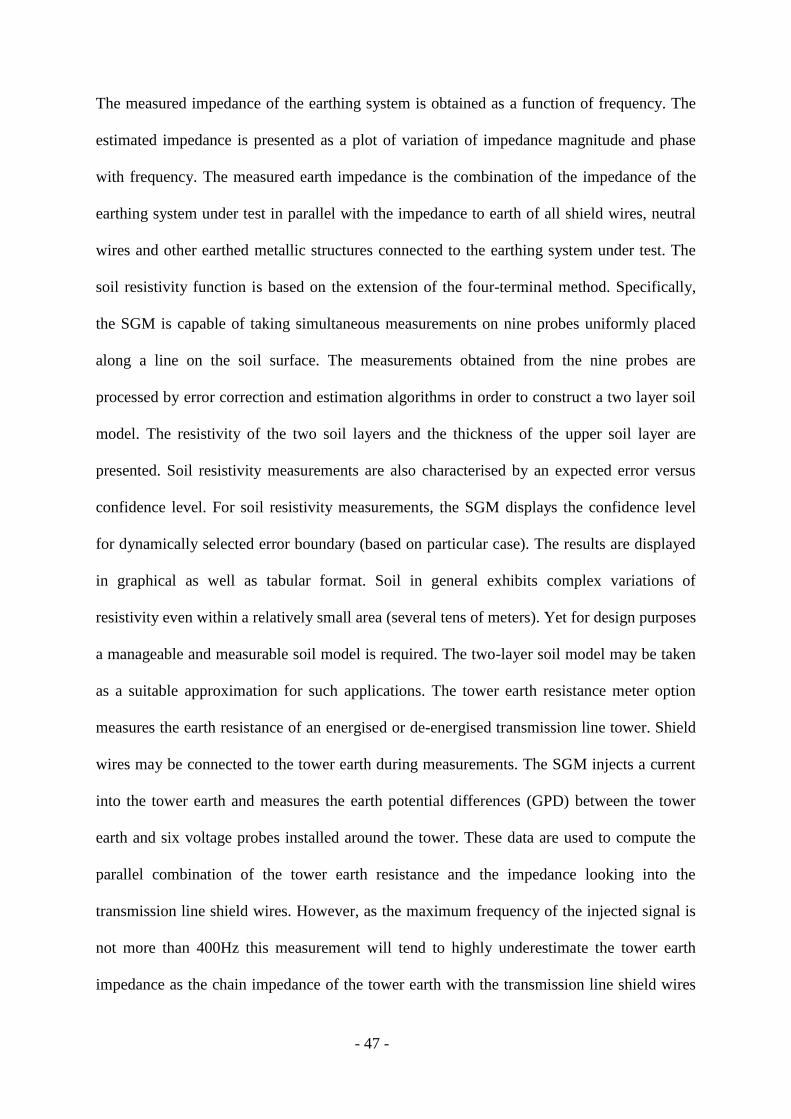
- 47 -
The measured impedance of the earthing system is obtained as a function of frequency. The
estimated impedance is presented as a plot of variation of impedance magnitude and phase
with frequency. The measured earth impedance is the combination of the impedance of the
earthing system under test in parallel with the impedance to earth of all shield wires, neutral
wires and other earthed metallic structures connected to the earthing system under test. The
soil resistivity function is based on the extension of the four-terminal method. Specifically,
the SGM is capable of taking simultaneous measurements on nine probes uniformly placed
along a line on the soil surface. The measurements obtained from the nine probes are
processed by error correction and estimation algorithms in order to construct a two layer soil
model. The resistivity of the two soil layers and the thickness of the upper soil layer are
presented. Soil resistivity measurements are also characterised by an expected error versus
confidence level. For soil resistivity measurements, the SGM displays the confidence level
for dynamically selected error boundary (based on particular case). The results are displayed
in graphical as well as tabular format. Soil in general exhibits complex variations of
resistivity even within a relatively small area (several tens of meters). Yet for design purposes
a manageable and measurable soil model is required. The two-layer soil model may be taken
as a suitable approximation for such applications. The tower earth resistance meter option
measures the earth resistance of an energised or de-energised transmission line tower. Shield
wires may be connected to the tower earth during measurements. The SGM injects a current
into the tower earth and measures the earth potential differences (GPD) between the tower
earth and six voltage probes installed around the tower. These data are used to compute the
parallel combination of the tower earth resistance and the impedance looking into the
transmission line shield wires. However, as the maximum frequency of the injected signal is
not more than 400Hz this measurement will tend to highly underestimate the tower earth
impedance as the chain impedance of the tower earth with the transmission line shield wires

- 48 -
connected to the other towers. This measurement will provide a significantly lower
impedance reading at a frequency of 400Hz. It is shown later in this thesis, in Fig. 5.28, that,
to estimate the tower earth resistance, a frequency of injected current will have to be more
than 30kHz. This is one of the limitations of Smart Ground Meter while trying to use it to
measure the tower earth resistance with shield wires connected. An identification algorithm
determines the contribution of the shield wires and eliminates this contribution from the
measured total impedance. The algorithm is based on the observation that the shield wire
impedance is predominantly reactive while the tower earth impedance is resistive. Moreover,
the shield wire resistance and reactance are functions of frequency. The algorithm takes
advantage of this frequency dependence to extract the tower earth impedance from the
measured data. The algorithm also provides the statistical measures of the measurement
accuracy, which is expressed in terms of expected error versus confidence level. The
presented results consist of the tower earth impedance plotted as a function of frequency. The
touch and step voltage function measures the actual touch and step voltage at a substation as a
function of the fault current. The measurement is performed at up to six points near the
earthing system. A required input for this function is the fault current available at the location
of the earthing system. The data analysis takes into consideration the effect of the proximity
of the current return electrode on the measured touch and step voltages. The additional data
required for this measurement function are the co-ordinates of the voltage probes, current
return electrode and approximate size and shape of the earthing system.
A personal computer is used to compute the values of potential gradients and current at
various locations to generate the values of earth impedances at various frequency levels. The
signal acquisition unit acquires, filters and attenuates the signals to the suitable level for
further processing. There is also a current source unit which circulates the test current into the
earth electrode under test. There are six voltage probes with a set of three voltage probes each

- 49 -
in an insulated flexible conduit. These probes are used for recording the potential at various
points in relation to the earth under test. It also consists of one assembly of current return
electrode.
2.5 Effect of pin spacing on the measured earth impedance
The minimum geographical extent required to measure the earth impedance with sufficient
accuracy (linear pin spacing required between the injection electrode and the return current
electrode and the orthogonal pin spacing required between the injection electrode and the
potential reference electrode) is of interest from the point of view of area constraints faced
during the measurement of the large area earth electrodes. The effect of pin spacing on the
earth resistance depends on the geometrical extents of the earthing electrode and the soil
resistivity pattern of the site of earthing [63]. Wenner 4-pin measurement method is generally
used to interpret the layered soil resistivity at the site. It is generally known that larger the
Wenner pin spacing, higher the depth of the soil resistivity sensed. To study the effect of pin
spacing on the measured earth resistance Southey et al. [63] performed computer simulations
based on the measured soil resistivites with different pin spacings and substituted these
values in the computer program to estimate the earth resistance. They considered 152m x
152m earth grid and the two double layer soil resistivity models such as a) 100Ωm layer over
5000Ωm and b) 5000Ωm layer over 100Ωm. They computed grid earth resistance as a
function of top layer thickness sensed by the resistivity measurements. The % error in the
computed grid resistance and safety voltages observed by them is shown in Figure 2.10.

- 50 -
(a) Error in grid perfromance predictions versus maximum pin spacing: 100 Ωm soil layer,
30m (100ft) thick, over 5000 Ωm soil.
(b) Error in grid perfromance predictions versus maximum pin spacing: 100 Ωm soil layer,
152m (500ft) thick, over 5000 Ωm soil.

- 51 -
(c) Error in grid perfromance predictions versus maximum pin spacing: 5000 Ωm soil layer,
30m (100ft) thick, over 100 Ωm soil.
Figure 2.10 Percentage error in computed grid resistance as a function of pin spacing [63]
They concluded that with the resistivity ratios varying from 1:50 and 50:1 (extreme cases
expected in the field) between two layers, the maximum error in the computed grid resistance
depends on the depth of the top layer and maximum pin spacing as shown in Table 2.3.
Table 2.3 Computed grid resistance error range
Maximum pin spacing (% of grid length) Maximum computed grid resistance error
range
40% -50% to +30%
100% -33% to +9%
300% -17% to +(<9%)
From the study conducted by Southey et. al, it can be concluded that for the high over low
resistivity layer model, the pin spacing (between the injection current electrode and return
current electrode) of more than 3 times the maximum grid length is sufficient to minimise the
error within +9% for the computed grid resistance. For the converse resistivity model (low

- 52 -
over high resistivity layer, with deeper top layer), it is desirable to have the pin spacing
(between the injection current electrode and return current electrode) close to 10 times the
maximum grid length to minimise the error (<-10%) in the computed earth resistance. The
pin spacing between the injection electrode and the potential reference electrode is desired to
be such that the potential reference electrode is outside the zone of influence of the earth
electrode under test.
2.6 Conclusion
The literature review revealed that the most reliable method of measurement of earthing
impedance of the practical earth electrodes is the Fall of Potential Method. This method has
been widely used by the commercially available earth resistance measurement testers.
However it is time consuming and labour intensive. Therefore different other methods of
measurements such as three point method, ratio method, clamp-on earth testing method are
used to measure the impedance of earthing system. The behaviour of earth impedance
measurement at the power frequencies has been studied in considerable details in the past and
has led to the development of robust techniques for the measurement of earthing impedance
at power frequencies. Several efforts were also made by the authors in the past and are being
made at present to characterise the behaviour of earthing systems under high frequency and
impulse conditions. However, to know to complete extent, the behaviour of earthing systems
under transient impulse and high frequency conditions it would require further investigation.
These findings will help us propose the suitable measurement techniques to measure the earth
impedances which will be representative at the lightning transient and impulse conditions. It
was noted that the Smart Ground Meter will provide underestimation of the values of the
tower earth resistance as the injected signal from the Smart Ground Meter is less than 400Hz.
This limitation of Smart Ground Meter can be overcome by using a suitable current signal

- 53 -
injection source with a frequency of the order of few tens of kHz. The literature review has
also revealed that the effect of electromagnetic coupling between the test leads, interference
with the leakage power frequency currents circulating in the earthing system and the spacing
between testing electrodes may affect the measurement. Due care is required to be taken to
reduce the error introduced by these aspects. Moreover, in this chapter, the survey of earthing
measurement techniques was carried out, the limitations and advantages of the commercially
available earth testers has been identified and the range of applications of these earth testers
have been determined.

- 54 -
Chapter 3: Determination of accuracy of transducers and
preliminary laboratory tests
3.1. Introduction
The experimental programme in this thesis required the use of several voltage and current
transducers. These transducers were tested in the laboratory with the variable frequency /
voltage / current sources to ascertain their accuracy and characterise their response. The
objective of this exercise was to verify the suitability of the transducers and apply correction
factors if necessary to the values obtained during the experimental campaign. The laboratory
tests were performed on the earth resistance testers to measure the standard resistance.
Laboratory tests were also performed on the conduction mediums such as dry sand, wet sand,
tap water and distilled water to see the behaviour of these mediums to the variable frequency
and variable magnitude current signals.
3.2. Voltage transducers
The voltage transducers used in the test were differential voltage attenuators. Differential
voltage measurement was required to decouple the electronics measurement systems from the
power frequency noise present in the earthing systems under test. Attenuation was necessary
to bring the level of the measured signals to sufficiently lower amplitudes compatible with
the electronics measurement systems. The technical specifications of SI 9000 and Chauvin
Arnoux make DP25 voltage probes are as follows. The accuracies of both the potential
transducers is specified as 2%. The selectable attenuation values are 20 and 200 for the
SI9000 voltage probe and 20, 50 and 200 for the DP25 voltage probe. The input impedance is
2MΩ/2.5pF for the SI9000 voltage probe and 4MΩ/1.2pF for the DP25 voltage probe. The
3dB bandwidth of SI9000 and DP25 voltage probes is DC to 25MHz and DC to 15MHz

- 55 -
respectively. Both the voltage probes are capable of measuring a voltage signal of fastest rise
time up to 24nS. The maximum input to ground voltage capability of SI 9000 is 700V RMS
at attenuation setting of 200 and 70V RMS at attenuation setting of 20. DP25 is capable of
measuring maximum of 600V RMS between input to ground at all the attenuation settings.
Appendix A1 gives the detailed specifications of the voltage probes tested in the laboratory.
The test setup used during laboratory tests on transducers is shown in Figure 3.1 and the test
results are shown in the Figure 3.2 and Figure 3.3.
Figure 3.1 Test setup for calibration of differential probes
A standard signal generator was used with test voltages in the range of 0-5V and frequencies
over the range 20 Hz to 1MHz as a source. Output of the signal generator was directly fed
into a duly calibrated Lecroy oscilloscope (Waverunner 64xi) to measure the input voltage
level. The output of the differential voltage attenuator transducer was fed into the channel 2
of oscilloscope. The two signals were compared. Figure 3.2 and Figure 3.3 shows the
percentage error of the signal for the output of the transducer compared with the direct signal
measurement.

- 56 -
Figure 3.2 Determination of the accuracy of the voltage transducer SI 9000 serial number 26950
Figure 3.3 Determination of the accuracy of the voltage transducer DP25 serial number 20080843
The transducers were tested over a frequency range 20 Hz to 1 MHz. The different potential
transducers tested had a measured error of less than ± 3% over a complete frequency range.
These calibration curves obtained were used to apply the correction factors to the values of
measured voltages during the experiments.

- 57 -
3.3. Current transducers
A comparison of the frequency response of different current transducers was made. The
transducers included LILCO CT, Stanganes current transformers and Tektronix make current
probes. In the test set up shown in Figure 3.4 the current transducers to be compared were
used for measuring the same current generated by a standard signal generator over the
frequency range 20 Hz to 10 MHz.
Figure 3.4 Test set up for comparison of current transducers
The current transducers were tested in four groups as shown in the Table 3.1.
Table 3.1 Groups of current transducers formed for testing purpose
Group No. Current transducers included in the group
Group No. 1 LILCO CT and Tektronix current probe
Group No. 2 Tektronix probe, Stanganes CT serial nos. 12316, 13370 and 13971.
Group No. 3 LILCO CT and Stanganes CT serial nos. 8042 and 8043
Group No. 4 LILCO CT and Stanganes CT serial nos. 8042, 8043 and 13967
The current transducers were grouped to a maximum number of four to facilitate waveform
measurements on the four channel Lecroy oscilloscope. Same current was passed through the
current transducers in each group to measure their response to current magnitude and
frequency. LILCO CT and Tektronix current probes are wide bandwidth transducers while
the Stanaganes CT’s were the pulsed CT’s. The detail specifications of the current
transducers is provided in the Appendix A1. The LILCO CT and Tektronix current probe

- 58 -
were tested over a wide band of frequencies 20Hz to 200kHz. The Stanganes CT’s were
tested over a frequency range of 1kHz to 1MHz. LILCO CT was used to measure the
standard cropico resistance for a low frequency response. The accuracy of LILCO CT was
found to be highest during the test with the standard resistance measurement. Hence LILCO
CT was used as a reference for comparison of the other current transducers.
Output responses of different current transducers is shown in the Figure 3.5. As seen from
Figure 3.5, the response of the current transducers was in close agreement over the frequency
range 20Hz to 200kHz and 1kHz to 1MHz.
Figure 3.5 Comparison of current transducers
The Stanganes current transformers showed accuracies close to the LILCO CT (less than 2%
error was observed), while the Tektronix probes were comparatively less accurate (about 6%
error was observed). The majority of the subsequent field experiments were performed using
the LILCO CT.

- 59 -
3.4. Laboratory tests of earth resistance meters and earth impedance measurement
system (IMS)
Calibrated resistances using a CROPICO make standard resistance were measured with a
Megger earth resistance tester DET 2/2, the Cardiff University make Impedance
Measurement System (IMS) [42] employing the lock-in amplifiers and the ABEM
Terrameter.
3.4.1. DET 2/2 laboratory tests
The Cropico make standard resistance MTS1A at 1Ω, 1.9Ω and 10Ω settings was measured
with Megger make DET2/2 earth resistance tester. As seen from Figure 3.6, Figure 3.7 and
Figure 3.8, the measured value of resistance was found to be accurate within 0.2 % of the
standard value. DET 2/2 has a facility to measure the DC earth resistance at a low DC
switching frequencies ranging from 105Hz to 160Hz.
0.96
0.97
0.98
0.99
1
1.01
100 110 120 130 140 150 160
Re
sis
tan
ce
(Ω
)
Frequency (Hz)
Figure 3.6 Measurement of Cropico MTS1A standard 1Ω resistance with DET 2/2

- 60 -
1.86
1.87
1.88
1.89
1.9
1.91
100 110 120 130 140 150 160
Resis
tan
ce
(Ω
)
Frequency (Hz)
Figure 3.7 Measurement of Cropico MTS1A standard 1.9Ω resistance with DET 2/2
9.6
9.7
9.8
9.9
10
10.1
100 110 120 130 140 150 160
Re
sis
tan
ce
(Ω
)
Frequency (Hz)
Cropico MTS1A, 10 ohm resistance
Figure 3.8 Measurement of Cropico MTS1A standard 10Ω resistance with DET 2/2
3.4.1. IMS laboratory tests
Figure 3.9 shows the measurement of 1Ω standard resistance with the Cardiff University
make IMS over the frequency range 80Hz to 1kHz. As seen from the Figure 3.9 the measured
resistance value is close to 0.9825Ω over the freqncy range 80Hz to 1kHz.
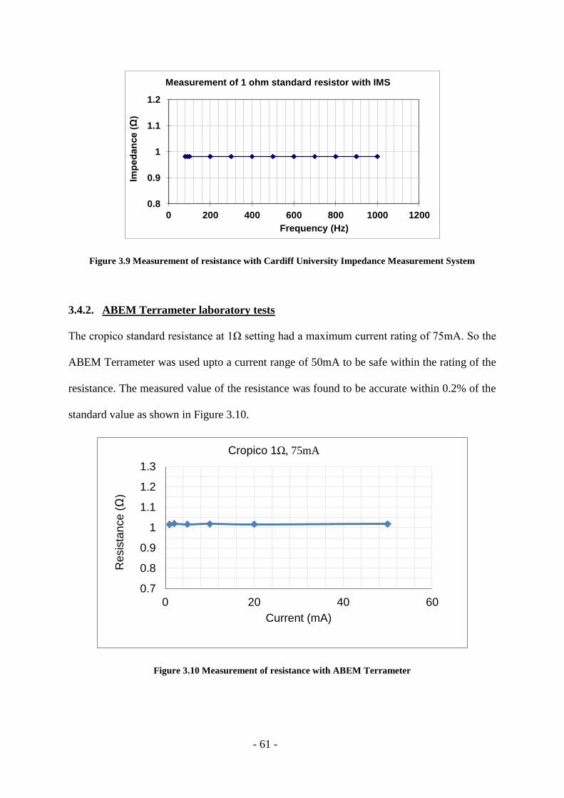
- 61 -
0.8
0.9
1
1.1
1.2
0 200 400 600 800 1000 1200
Frequency (Hz)
Measurement of 1 ohm standard resistor with IMS
Imp
ed
an
ce (
Ω)
Figure 3.9 Measurement of resistance with Cardiff University Impedance Measurement System
3.4.2. ABEM Terrameter laboratory tests
The cropico standard resistance at 1Ω setting had a maximum current rating of 75mA. So the
ABEM Terrameter was used upto a current range of 50mA to be safe within the rating of the
resistance. The measured value of the resistance was found to be accurate within 0.2% of the
standard value as shown in Figure 3.10.
0.7
0.8
0.9
1
1.1
1.2
1.3
0 20 40 60
Resis
tan
ce
(Ω
)
Current (mA)
Cropico 1Ω, 75mA
Figure 3.10 Measurement of resistance with ABEM Terrameter

- 62 -
3.1 Laboratory tests of impedance measurements of soil and electrolytes
Figure 3.11 shows the experimental test set up of the impedance measurement tests
performed in the laboratory controlled environment.
Figure 3.11 Test set-up for laboratory tests on the soil and water.
The objective of these tests were to observe the effect of frequency and current magnitude on
the impedance of distilled water, dry sand, wet sand and tap water respectively. The test cell
was 200mm x 200mm x 200mm (length x breadth x height). The height of the medium
(distilled water / dry sand / wet sand / tap water / electrolyte solution) with which the test cell
was filled was 160mm. The space above the level of 160mm would introduce some stray
capacitance. However, it was found that this stray capacitance is negligible.
Various conducting mediums such as dry sand, 3.24% wet sand, tap water and distilled water
were tested for the measurement of the impedance at frequencies over the range of 20Hz to
100kHz. The current magnitudes were also varied from few milli-amperes to few hundred
milli-amperes. The effect of frequency and the AC / DC current magnitudes was studied
during the experiments performed on the test cell at the Cardiff University laboratory.

- 63 -
Figure 3.12 shows the effect of frequency on the measured impedance of the 3.24% wet sand
filled in the test cell. As seen from the figure there is about 10% reduction in the measured
earth impedance over the frequency range 20Hz to 100kHz. The plots in different colours
denote the impedances observed over the current range 39mA to 780mA.
Figure 3.12 Effect of frequency on the impedance of 3.24% wet sand filled in the test cell
Figure 3.13 shows the effect of frequency on the measured impedance of the dry sand filled
in the test cell. As seen from the figure there is about 30% reduction in the measured earth
impedance over the frequency range 20Hz to 100kHz. The plots in different colours denote
the impedances observed over the current range 3.7mA to 84.9mA.
0
10
20
30
40
50
60
70
80
10 100 1000 10000 100000Frequency (Hz)
3.24% wet sand (39mA to 780mA)
Imp
ed
an
ce (
Ω)
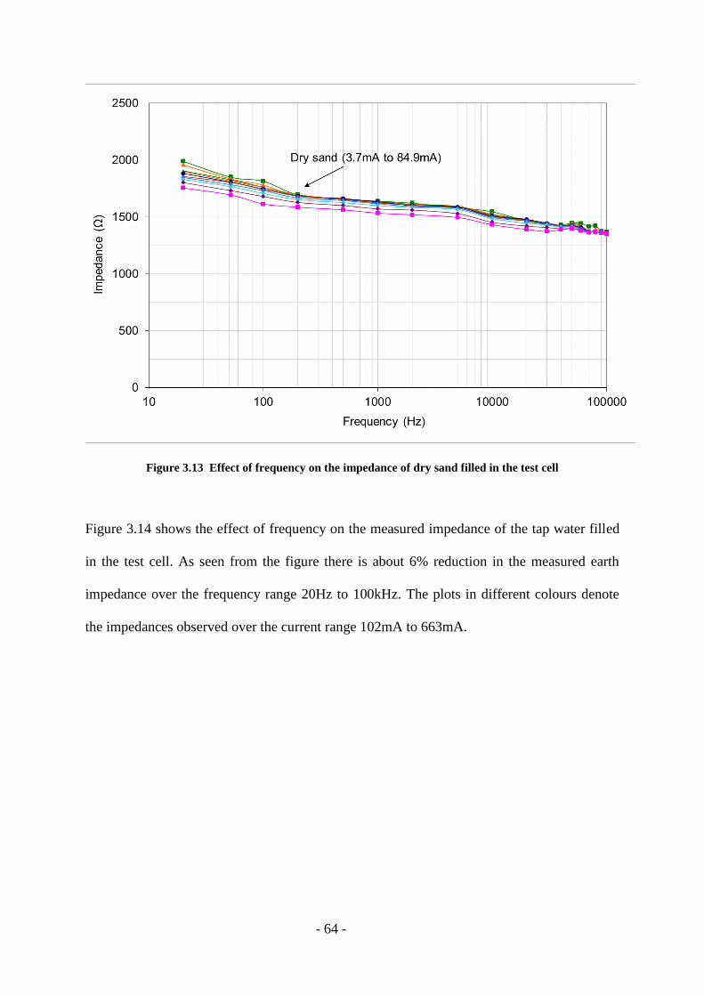
- 64 -
Figure 3.13 Effect of frequency on the impedance of dry sand filled in the test cell
Figure 3.14 shows the effect of frequency on the measured impedance of the tap water filled
in the test cell. As seen from the figure there is about 6% reduction in the measured earth
impedance over the frequency range 20Hz to 100kHz. The plots in different colours denote
the impedances observed over the current range 102mA to 663mA.

- 65 -
Figure 3.14 Effect of frequency on the impedance of tap water filled in the test cell
Figure 3.15 shows the effect of frequency on the measured impedance of the distilled water
filled in the test cell. As seen from the figure there is about 40% reduction in the measured
earth impedance over the frequency range 20Hz to 100kHz. The plots in different colours
denote the impedances observed over the current range 0.52mA to 11.82mA.

- 66 -
Figure 3.15 Effect of frequency on the impedance of distilled water filled in the test cell
As can be seen from Figure 3.16, there is order of magnitude difference between the
measured impedance / resistance of distilled water, dry sand, wet sand and tap water. The
impedance was measured at different frequencies with the IMS system while the DET 2/2
was used to measure the resistance of these mediums.
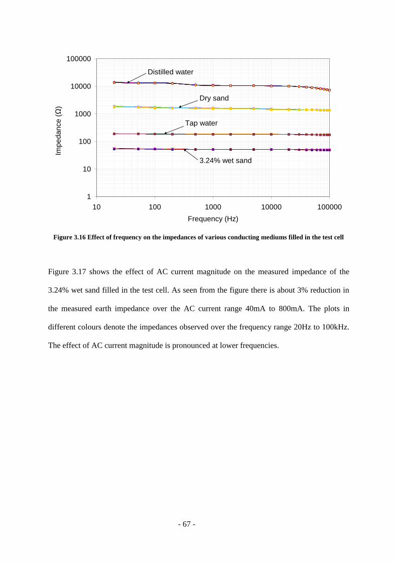
- 67 -
1
10
100
1000
10000
100000
10 100 1000 10000 100000
Frequency (Hz)
Distilled water
Dry sand
3.24% wet sand
Tap water
Imp
ed
an
ce
(Ω
)
Figure 3.16 Effect of frequency on the impedances of various conducting mediums filled in the test cell
Figure 3.17 shows the effect of AC current magnitude on the measured impedance of the
3.24% wet sand filled in the test cell. As seen from the figure there is about 3% reduction in
the measured earth impedance over the AC current range 40mA to 800mA. The plots in
different colours denote the impedances observed over the frequency range 20Hz to 100kHz.
The effect of AC current magnitude is pronounced at lower frequencies.

- 68 -
Figure 3.17 Effect of current magnitude on the impedance of 3.24% wet sand filled in the test cell
Figure 3.18 shows the effect of AC current magnitude on the measured impedance of the tap
water filled in the test cell. As seen from the figure there is about 6% reduction in the
measured earth impedance over the AC current range 40mA to 650mA. The plots in different
colours denote the impedances observed over the frequency range 20Hz to 100kHz. The
effect of AC current magnitude is pronounced at lower frequencies.

- 69 -
Figure 3.18 Effect of current magnitude on the impedance of tap water filled in the test cell
Figure 3.19 shows the effect of AC current magnitude on the measured impedance of the dry
sand filled in the test cell. As seen from the figure there is about 10% reduction in the
measured earth impedance over the AC current range 4mA to 80mA. The plots in different
colours denote the impedances observed over the frequency range 20Hz to 100kHz. The
effect of AC current magnitude is pronounced at lower frequencies.

- 70 -
Figure 3.19 Effect of current magnitude on the impedance of dry sand filled in the test cell
Figure 3.20 shows the effect of AC current magnitude on the measured impedance of the
distilled water filled in the test cell. As seen from the figure there is about 10% reduction in
the measured earth impedance over the AC current range 40mA to 800mA. The plots in
different colours denote the impedances observed over the frequency range 20Hz to 100kHz.
The effect of AC current magnitude is pronounced at lower frequencies.

- 71 -
Figure 3.20 Effect of current magnitude on the impedance of distilled water filled in the test cell
Figure 3.21 and Figure 3.22 show the effect of DC / AC current magnitude on the measured
values of the impedance / resistance of the various mediums tested in the laboratory at
Cardiff University.

- 72 -
10
100
1000
10000
100000
0.0001 0.001 0.01 0.1 1
Current (A)
Distilled water (ABEM)
3.24% wet sand (ABEM)
Tap water (ABEM)
Distilled water (DET 2/2)
Tap water (DET 2/2)
3.24% wet sand (DET 2/2)
Dry sand (DET 2/2)Dry sand (ABEM)
Imp
ed
an
ce
(Ω
)
Figure 3.21 Effect of DC current magnitude on the impedance of different current mediums filled in the
test cell
10
100
1000
10000
100000
0.0001 0.001 0.01 0.1 1
Current (A)
Distilled water @ 52Hz
3.24% wet sand @ 52Hz
Tap water @ 52Hz
Dry sand @ 52Hz
Imp
ed
an
ce
(Ω
)
Figure 3.22 Effect of AC current magnitude on the impedance of different current mediums filled in the
test cell

- 73 -
It was observed that the effect of current magnitude was higher (close to 20% variation in the
impedance of tap water and wet sand over the current range from 1mA to 500mA) in the case
of DC currents as seen from the Figure 3.21 (measurement with ABEM instrument).
Figure 3.23 shows the effect of frequency on the measured impedance of distilled water with
different electrolyte concentration.
Figure 3.23 Variation of impedance of water with frequency
It was observed that as the frequency increases the capacitive effect dominates and the
impedance of distilled water with less concentration of the electrolyte tends to merge towards
the resistance value at the higher frequencies of around 120 kHz. The capacitive reactance
part of the impedance was calculated from the measured phase angle between the voltage and
current for the different frequencies over the range 20Hz to 120kHz. At frequencies close to
120kHz the measured impedance values of the electrolyte solution are close to each other as
both the effects (reduction of the capacitive reactance as well as the sharp reduction of the
0
2000
4000
6000
8000
10000
12000
14000
10 100 1000 10000 100000 1000000
Frequency (Hz)
Imped
ance
(Ω
)
Distillled water
1 drop
2 drops
11 drops
3 drops

- 74 -
resistivity with frequency) seems to be playing the role in reducing the measured impedance
of the electrolyte solution. The effect of frequency on the resistivity of the water is shown in
Figure 3.24.
Figure 3.24 Variation of resistivity of water with frequency
The resistive component of the impedance was computed from the phase angles of the
measured voltages and currents. It was noted that the resistivity of the distilled water with
different electrolyte concentration reduced with increase in the frequency. The effect was
more pronounced for the higher resistivity case.
0
500
1000
1500
2000
2500
10 100 1000 10000 100000 1000000
Frequency (Hz)
Distilled water Distilled water + 1 drop of electrolyte
Distilled water + 2 drops of electrolyte Distilled water + 3 drops of electrolyte
Distilled water + 4 drops of electrolyte Distilled water + 5 drops of electrolyte
Distilled water + 6 drops of electrolyte Distilled water + 7 drops of electrolyte
Distilled water + 8 drops of electrolyte Distilled water + 9 drops of electrolyte
Distilled water + 10 drops of electrolyte Distilled water + 11 drops of electrolyte
Res
isti
vit
y (
Ω-m
)

- 75 -
Figure 3.25 shows the percentage change in the resistivity of the distilled water with
electrolyte solution when the frequency of the injected current signal is varied from 20Hz to
120kHz. As seen from Figure 3.25 the effect of frequency on the resistivity of electrolyte
solution is higher when the concentration of electrolyte is less or in other words it seems from
the laboratory experiments with distilled water and electrolyte solution, that the higher
impedance medium exhibits higher effect of frequency in the range 20Hz to 120kHz.
Figure 3.25 Percentage change in resistivity of water with frequency from 20Hz to 120kHz with
increasing electrolyte concentration
The impedance / resistance of the distilled water was gradually reduced with addition of the
drops of the electrolyte.
The laboratory measurement of the impedances and the calculation of the resistivities of the
conducting mediums from the experiments have shown that there is an effect of frequency on
the impedance and resistivity of the conducting mediums tested. A small effect of the DC
current magnitude was also seen on the resistance of the conduction mediums during the
experiments.
0
5
10
15
20
25
30
35
0 2 4 6 8 10 12
Number of drops of electrolyte
% change in resistivity from 20Hz to 120kHz with number of drops of electrolyte
Ch
an
ge
in
re
sis
tivity (
%)

- 76 -
3.2 Conclusion
The differential voltage transducers were calibrated over the frequency range of 20Hz to
1MHz in the laboratory and their errors were found to be within the range of specifications.
The output of current transducers were compared and found to be in close agreement over the
frequency range 20Hz to 200kHz and 1kHz to 1MHz. The commercially available earth
testers such as DET 2/2, ABEM Terrameter were used to measure the Cropico make standard
resistance in the laboratory and it was found that the measurement was in good agreement
with the standard resistance value. Subsequent to calibration of the voltage and current
transducers, and the commercial earth testers, an experimental measurement campaign for
soil and water resistance, was carried out in the laboratory environment. The measurement of
four different mediums such as dry soil, wet soil, distilled water and tap water was performed
over a frequency range of 20Hz to 100kHz. It was found that there was a noticeable decrease
(up to 30%) in measured impedance of these four mediums over a frequency range 20Hz to
100kHz. Moreover, the experiments for the measurement of the effect of AC/DC current
magnitude on the measured impedance of these four mediums were also performed. It
revealed that the effect of AC current on the measured impedance over the range of current
magnitude from 1mA to 1A was less than 3%. However, the DC current magnitude of 1mA
to 5mA showed a significant reduction (20%) of the measured impedance of the mediums
such as wet sand and tap water. Further tests were also performed on the distilled water and
distilled water mixed with electrolyte solution gradually increasing the conductivity of the
distilled water after each set of measurements of the impedance over a frequency range of
20Hz to 120kHz. These tests revealed slight reduction in the resistivity of the relatively high
conductivity water solution over the frequency range of 20Hz to 120kHz. However, a
significant reduction in the resistivity of distilled water was observed over the frequency
range 20Hz to 120kHz. It is shown in Chapter 7.4 (Figure 7.4) that the conductivity
- 77 -
dispersion observed in the laboratory experiments by Arulanandan [46] and modelled by
Oliver de Lima et al. [45] showed about 33% increase in conductivity of the soil water
electrolyte solution when subjected to increase in frequency in the range 100Hz to 100kHz.
Arulanandan [46] conducted experiments on saturated kaolinite clay-water-electrolyte
systems and found that there are two distinct dispersions, one in the low frequency range (0
to 100 kHz) and the other in the high frequency range (1 MHz to 100 MHz). An increase in
electrical conductivity has also been experimentally observed for clays by [47], [48], [49],
mineralised rocks [50], polymers [51], synthetic membranes [52], ion exchange resins [53]
and polystyrene spheres [54]. The conductivity dispersion characteristics were experimentally
observed in the frequency range of either 0 to 100 kHz or 1 MHz to 100 MHz.

- 78 -
Chapter 4: Description of test sites and facilities
The Cardiff University-developed earth impedance measurement system injects sinusoidal
signal into the earth electrode and captures the earth potential rise to compute the earth
impedance. The measurements performed with the sinusoidal signals near power frequencies
represent the earth impedance values for the power frequency conditions. However, to
measure the earth impedances representative of the lightning frequency and transient surge
conditions, a separate set of measurements is required to be performed at sinusoidal currents
at higher frequencies. In order to study the response of earthing systems, a series of earth
impedance/resistance measurement tests were conducted on different types of earthing
systems including rods, rod clusters, grid, tower base, horizontal electrode and tower line.
AC/switched DC/impulse energisation sources were used in this work to obtain earth
resistance/impedance values of the different systems at different frequency/current
magnitudes and impulse wave shapes. Two outdoor test sites were used; (i) Llanrumney
fields, where a number of earth test electrodes have been installed and (ii) Dinorwig Power
Station lower reservoir.
4.1. Overview of Llanrumney fields test site
Figure 4.1 shows a satellite image of the Cardiff University test field at Llanrumney. As seen
from Figure 4.1, the Llanrumney test site has purpose-built earthing systems such as (i) a 3m
x 3m earthing grid, (ii) a ring earthing system consisting of 8 single earth rods with a
provision to connect them together with a 25 mm2 bare or insulated copper conductor ring.
Each rod has dimensions of 16mm diameter and a length of 2.4m. The bare / insulated copper
conductors are buried approximately 20cm in the earth. The test site also includes in the
centre of the ring a purpose built tower base and an operational 275kV National Grid

- 79 -
transmission tower VP9 (which is not visible in the satellite image) approximately 100m
away from the test tower base.
Figure 4.1 Plan view of University test site at Llanrumney showing outline of installed test electrodes
Figure 4.2 shows the dimensions of the tower footing, the steel reinforcement bars and the
surrounding concrete structure. The distance between the leg stubs on the ground surface is
7m. The tower base is located at the centre of the ring electrode as shown in Figure 4.1. Each
leg of the tower base is a ‘L’ cross-section with the dimensions as shown in the section ‘A-A’
of Figure 4.2. The plan view of four legs of the tower base is shown in Figure 4.3.
The dimensions of the 3m x 3m grid are shown in Figure 4.4. It is made up of a 4 mesh (1m x
1m size) of copper tape with cross section 50mm x 6mm and 2.4m long vertical rods installed
at each corner. The horizontal grid conductors are 3m long.

- 80 -
Figure 4.2 Tower footing construction of one leg of tower base
Figure 4.3 Plan view of the four legs of the Tower base

- 81 -
Figure 4.4 Isometric view of 3m x 3m grid
The Ring Earthing system is made up of 8 rods having 16mm Ø and 1.2m long vertical rods
installed along the periphery of the circle with a 58m diameter. The plan view of ring
earthing system is shown in Figure 4.5.
Figure 4.5 Plan view of ring earthing system

- 82 -
A combination of concentrated and extended earthing systems can be realised from the
individual earthing electrode components at Llanrumney test field. This provides the
opportunity to measure the earth impedance of the following earthing systems
1) Single earth rod – 16 mm ø, 2.4m length
2) 3m x 3m, 4 mesh earth grid
3) 275kV purpose built tower base
4) 275kV National Grid operational tower base VP9 and extended tower line
earthing system
5) Parallel combination of vertical rods connected with insulated copper cable
6) Parallel combination of vertical rods connected with the bare copper cable
forming a horizontal electrode plus vertical electrode arrangement
7) Extended electrode comprising the 275kV purpose built tower base in parallel
with the ring earth electrode (when all the 8 vertical rods are connected with
bare copper cables)
The purpose of the tests at Llanrumney was to study the behaviour of the earthing systems
under the influence of various energisation such as variable current DC / AC, variable
frequency and impulse current injection.
4.2. Overview of Dinorwig test site
Earth impedance measurements performed on earthing systems buried in the soil at
Llanrumney provides representative practical conditions to investigate the behaviour of the
earthing systems at different energisation conditions. However, the soil medium at this test
site is non-homogeneous with horizontally and vertically layered resitivities of the soil
structure. It is well known that the conduction of electric current in the soil is mainly
electrolytic in nature and occurs through the water molecules in the micro-pores of the soil

- 83 -
structure. Hence, it was decided to conduct experiments on test earth electrodes in a
homogenous water medium. The lower reservoir of Dinorwig pumped hydro power station
was chosen to conduct such experiments at it offered the potential of homogenous water
conditions. Dinorwig pumped-storage hydro-electric power station is located in Llanberis,
North Wales, UK. Figure 4.6 shows a plan view of the lower reservoir of the station, which is
approximately 1.8km long and 400m wide. The reservoir is characterised by steep sides and a
relatively flat bottom. The reservoir water level varies over a range of about 15m and, from
power station records, the water level at any given time can be ascertained accurately.
Figure 4.6 Plan of the lower reservoir at Dinorwig power station showing water resistivity test locations
4.2.1. Water resistivity measurements
Initial water resistivity measurements were carried out at positions close to the shore on
09/05/2007, 19/07/2007. Further detailed measurements were carried out on
30/07~01/08/2007 to investigate variations in water resistivity and temperature at different
locations on the lake and also with water depth.
- 84 -
The water resistivity test locations are illustrated in Figure 4.6. Location was chosen as it
corresponds to the central position of the proposed test electrode area. Location is close to
the down-stream outlet while Location is inside the ‘Wellington channel’, the main
channel for the power station. Finally, Locations and were chosen to investigate
resistivity where the water may be less mixed. Location is at the end of the slip road. At
Locations , and , detailed measurements were taken at different depths from the water
surface. At the other locations, readings were taken approximately 0.5m below water
surface.
4.2.2. Resistivity measurement survey on 09/05/2007
Due to the significant rise in the water level of the lake and to prevent the probe of the
resistivity instrument being caught up in the rocks of the lake bed, the probe was retrieved
frequently around Location , according to the water level rise. As a result, all the initial
measurements were restricted to the top layer of water with the probe at a depth of around 1
meter. A representative set of measurements taken on 09/05/2007 is listed in Table 4.1.
In Table 4.1, a log of measurements is shown for readings taken at 30 second intervals
followed by the temperature measured (T˚C). The fourth column shows the actual
conductivity results (S/cm). The fifth column shows the temperature-corrected (to 20˚C)
resistivity results (in Ωcm), based on the actual conductivity measurements. Salinity of the
water and atmospheric pressure are also recorded, shown in columns 6 and 7.

- 85 -
Table 4.1 Typical water resistivity measurement results on 09/05/2007
Date Time
Water
Temperature
(˚C)
Actual Water
Conductivity
(S/cm)
Water
Resistivity
(Ωm)
Salinity
(g/L)
Pressure
(kPa)
2007/05/09 14:15:25 15.22 74 122 0.04 99.78
2007/05/09 14:15:55 15.24 74 122 0.04 99.81
2007/05/09 14:16:25 15.25 74 123 0.04 99.81
2007/05/09 14:16:55 15.26 74 122 0.04 99.81
2007/05/09 14:17:25 15.23 74 123 0.04 99.80
2007/05/09 14:17:55 15.23 74 123 0.04 99.79
2007/05/09 14:18:25 15.23 74 122 0.04 99.79
2007/05/09 14:18:55 15.25 75 122 0.04 99.79
2007/05/09 14:19:25 15.25 75 122 0.04 99.81
4.2.3. Resistivity measurement survey on 19/07/2007
A second set of lake water resistivity measurements, again at Location , were taken on
19/07/2007 at the same position and depth with the first water resistivity measurement. A
rise of water temperature from around 15˚C to around 19~20˚C was recorded, and the actual
conductivity increased from around 74 S/cm to 76~80 S/cm. The water resistivity (after
temperature correction), conductivity and temperature are plotted in Figure 4.7 (a) and (b)
respectively.

- 86 -
(a) Water resistivity (after temperature correction) results
(b) Actual water conductivity measurement results
Figure 4.7 Water resistivity and conductivity measurement results on 19/07/2007
126.8
127
127.2
127.4
127.6
127.8
128
128.2
128.4
128.6
128.8
12:5
7:48
12:5
8:48
12:5
9:48
13:0
0:48
13:0
1:48
13:0
2:48
13:0
3:48
13:0
4:48
13:0
5:48
13:0
6:48
13:0
7:48
13:0
8:48
13:0
9:48
13:1
0:48
13:1
1:48
13:1
2:48
13:1
3:48
13:1
4:48
13:1
5:48
13:1
6:48
13:1
7:48
13:1
8:48
13:1
9:48
13:2
0:48
13:2
1:48
13:2
2:48
Time (hh:mm:ss)
Wat
er R
esis
tivity
(Ω·m
)
17.5
18
18.5
19
19.5
20
20.5
21
21.5
22
22.5
Tem
pera
ture
(°C
)
Watre Resistivity (Ω·m) T (°C)
71
72
73
74
75
76
77
78
79
80
81
12:5
7:48
12:5
8:48
12:5
9:48
13:0
0:48
13:0
1:48
13:0
2:48
13:0
3:48
13:0
4:48
13:0
5:48
13:0
6:48
13:0
7:48
13:0
8:48
13:0
9:48
13:1
0:48
13:1
1:48
13:1
2:48
13:1
3:48
13:1
4:48
13:1
5:48
13:1
6:48
13:1
7:48
13:1
8:48
13:1
9:48
13:2
0:48
13:2
1:48
13:2
2:48
Time (hh:mm:ss)
Wat
er C
ondu
ctiv
ity (µ
S/c
m A
)
17.5
18
18.5
19
19.5
20
20.5
21
21.5
22
22.5
Tem
pera
ture
(°C
)
Watre Conductivity (µS/cm A) T (°C)

- 87 -
4.2.4. Resistivity measurement survey on 01/08/2007
During the site visit 30/07~01/08/2007, a comprehensive set of water resistivity
measurements was carried out across the lake using the test boat. Table 4.2 lists the results
obtained on 01/08/2007 at test Location .
Table 4.2 Water resistivity measurement results on 01/08/2007
Date &
time
Probe
depth
(m)
Water
Resistivity
(Ωm)
Water
Temperature
(˚C)
Actual Water
Conductivity
(S/cm)
01/0
8/2
007
15:3
0 o
nw
ard
0.5 126 19.28 78
1 126 19.28 78
2 126 19.27 78
3 126 19.22 78
4 126 19.16 78
5 126 19.17 78
6 125 19.15 78
7 126 19.16 78
8 126 19.16 78
9 125 19.15 78
10 125 19.16 78
11 125 19.15 79
The results obtained from the water resistivity measurements taken over a period of three
days indicated that
The lake water resistivity varied between 125Ωm and 130Ωm

- 88 -
There was very little variation of resistivity with lake test location or with depth.
A slight reduction in temperature with depth (up to 0.2 ˚C per 10m) was noted.
The results of water resistivity measurements at the reservoir confirm that the water
resistivity and temperature on any given day is largely uniform, both depth-wise and area-
wise.
4.3. Experimental set up at Dinorwig Test Site
A cabin (as test base) was set up 50m from the reservoir, to the right of the station
administration building as shown in Figure 4.6. A motorboat was used to facilitate
installation of the test earthing systems in the reservoir and for carrying out the water
resistivity surveys. Vehicle and boat access to the water was obtained via a slip road.
To enable the test electrodes to be immersed in the lake at a fixed position, a pontoon was
constructed from the shore to the electrode test position. A side view of this construction is
shown in Figure 4.8. In this series of tests, two different test setups were adopted. The
purpose of these comparative tests was to determine whether there are differences in results
when locating the voltage sources a) in the test cabin or b) next to the test object.

- 89 -
Figure 4.8 Side view of the test set up at Dinorwig
Figure 4.9 shows the plan of test set up where the test objects were (a) A 14mm diameter
earth rod with 80cm immersed in water and (b) A 14mm diameter earth rod with 200cm
immersed in water.
Figure 4.9 Plan view of test set up 1 (injection source placed in the test cabin 150m away from the test
object)
Water level
Rod 1: Test object
Rod 2: Touch
voltage Reference
Current injection Lead
Potential measurement lead
Optical fibre
Water
Rock bed and shore
20m
Infin
ite
A total of 128m of floats
Test
Cabin
Earth return electrode

- 90 -
The source (IMS, RF, Impulse generator, DET 2/2 and ABEM terrameter) were placed in the
cabin. Injected current was measured with a Tektronix probe in the cabin. With all the test
instruments located in the test cabin, two channels of fibre optic links were used to enable the
measurement of current and touch voltage at the test electrode. The current measurement
was realised by the Lilco CT and fibre channel EYE and the touch voltage was measured
using DP25 (at 1/50) and fibre channel ‘ABB’. The attenuation of ‘EYE’ channel was
calibrated as 16 in lab but was recalibrated as 24.35 on site before laid out. The attenuation
of channel ABB was verified to be ‘32’, which is similar to previously obtained laboratory
result.
Figure 4.10 shows the plan view of the test set up where the source (IMS, RF, Impulse
generator, DET 2/2 and ABEM terrameter) were placed on the boat near the test object. In
this experiment a single vertical rod (14 mm dia. and 800 mm immersed in water) and the
horizontal tape (5m long and 506mm2 at cross section) were used as test objects.

- 91 -
Figure 4.10 Plan view of test set up 1 (injection source placed near the test object)
Figure 4.11 shows the view from the end of the pontoon towards the test cabin. It also shows
the outline of a 5m×5m grid test earth grid (diagonally oriented) beneath the water surface.
The white vertical poles are used to control the depth of the test electrode. The pontoon is
anchored at multiple positions to the lake bed and shore to maintain a fixed position.
Table 4.3 shows the list of earth electrodes, with dimensional details, tested at Dinorwig test
site. The commonly used geometries such as single earth rod, horizontal conductor and grid
earth electrodes were tested at Dinorwig to understand the behaviour of earth electrodes in
homogenous medium and energised with DC / AC / impulse voltages.
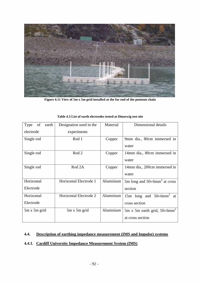
- 92 -
Figure 4.11 View of 5m x 5m grid installed at the far end of the pontoon chain
Table 4.3 List of earth electrodes tested at Dinorwig test site
Type of earth
electrode
Designation used in the
experiments
Material Dimensional details
Single rod Rod 1 Copper 9mm dia., 80cm immersed in
water
Single rod Rod 2 Copper 14mm dia., 80cm immersed in
water
Single rod Rod 2A Copper 14mm dia., 200cm immersed in
water
Horizontal
Electrode
Horizontal Electrode 1 Aluminium 5m long and 506mm2 at cross
section
Horizontal
Electrode
Horizontal Electrode 2 Aluminium 15m long and 506mm2 at
cross section
5m x 5m grid 5m x 5m grid Aluminium 5m x 5m earth grid, 506mm2
at cross section
4.4. Description of earthing impedance measurement (IMS and Impulse) systems
4.4.1. Cardiff University Impedance Measurement System (IMS)

- 93 -
The Cardiff University Impedance Measurement System comprises a variable frequency
signal generator (Perkin Elmer DSP lockin amplifier model 7225) coupled with power
amplifier (QSC PLX 2402) used as a signal source. A Lock-in Amplifier produces a DC
output proportional to the rms value of the AC measured signal. As can be seen in Figure
4.12, the input signal is amplified and then multiplied by the reference signal.
Figure 4.12 Principle of operation of lock-in amplifier
This multiplication process yields a series of signals involving the sum and difference
frequencies of the input and reference signals. If the required signal frequency equals the
reference signal frequency, the difference frequency component is a DC signal and can be
extracted using a low-pass filter. To obtain both amplitude and phase information, two lock-
in outputs are generated (X and Y). The X output is obtained from the product of the input
signal and the reference oscillator signal, while the Y output is derived from the product of
the input signal and the reference oscillator shifted by 90°. After filtering, these outputs
provide the in-phase and quadrature components respectively of the signal phasor, from
which the magnitude (R) and phase value (Φ) can be obtained. The power amplifier has
maximum output power of 2.4kW and, in bridge mode, provides an open circuit voltage of

- 94 -
120V. The output of the power amplifier drives the current into the earthing electrode under
test. Both the current injected into the system and the resulting earth potential rise are
measured with transducers and fed into the inputs of two lock-in amplifiers to calculate the
amplitude of the measured signals at a frequency of the reference signal. The lock-in
amplifiers also compute the phase of the current and Earth Potential Rise (EPR) signals with
respect to the reference signal.
Figure 4.13 shows the assembly of the Impedance Measurement System. A wide band current
transformer model (Lilco 58MH100) was used as the current transducer for field tests.
Figure 4.13 Impedance Measurement System
It has an output rating of 0.1V/A, frequency response 1.5Hz to 20MHz, a capacity to measure
RMS current of 100A, and 20ns response time. The minimum current measured during the
experiments was of the order of few mA. At the minimum current measured during the
experiments it provided a voltage output of few mV. It is to be noted that the IMS system has
a resolution to measure accurately the single level of few hundred microvolts. Differential
probe (SI9000) was used as the potential transducer. It has attenuation settings for 20 or 200,
an accuracy of 2%, an input impedance of 2MΩ, an input capacitance of 2.5pF, a frequency
- 95 -
range DC to 15MHz and a maximum voltage measurement capability of 700V DC / 500V
RMS.
4.4.2. Radio Frequency System (RF)
A Marconi Instruments signal generator 2019A was used as an input to the 25Watts CW,
10kHz to 250 MHz power amplifier to constitute a RF system. The Marconi make signal
generator 2019A has an output frequency range of 10kHz to 1040MHz with a resolution of
10Hz over a frequency range 10kHz to 520MHz and a resolution of 20Hz over a frequency
range of 520MHz to 1040MHz.
4.4.3. Impulse current injection system
A Haefley recurrent surge generator model RSG 481 is used as the signal source used for
impulse tests. The maximum impulse charging voltage of this surge generator is 500V on
open circuit which leads to a maximum test output voltage of approximately 400V. The
components of the impulse generator such as impulse and load capacitances, front and tail
resistors as well as inductances are adjustable in steps. The wave shape can thus be adjusted
over a wide range (depending on the load (earthing system under test) RLC parameters). The
maximum current injected into the earthing system under test depends on the energy stored in
the impulse capacitance and the load RLC parameters. The typical maximum current
obtained in the field with the recurrent surge generator was more than 5A with Test Tower
Base as load.
4.5. Measurement of resistivity at test site locations with ABEM Terramer
4.5.1. Measurement of Resistivity at Llanrumney fields

- 96 -
Based on previous extensive soil resistivity surveys performed along the survey lines as
shown in Figure 4.16, considerable data on soil resistivity for the Llanrumney test site has
been obtained.
In addition, two surveys were carried out during the present project. The soil resistivity
measurement results are shown in Figure 4.17 and Figure 4.18. The Wenner test set up as
shown in the Figure 4.14 was used to map the soil resistivity along the survey line R7 as
shown in Figure 4.16. Measurement of the ground resistivity was carried out by injecting a
controlled current (I) between two electrodes into the ground, while measuring the potential
(V) between two other electrodes. Direct current (DC) or an alternating current (AC) of very
low frequency is used, and the method is often called DC-resistivity. The resistance (R) is
calculated using Ohm's law: R = V / I. The Wenner configuration is a case where the four
electrodes are equally spaced with a separation distance ‘a’. Using the ABEM Terrameter
LUND Imaging System, multi-electrode gradient surveying was carried out by injecting
current with a separation (s+2)a and simultaneously or sequentially picking up all the
potential differences between the potential electrodes with the spacing a (Figure 4.15). Here,
‘s’ is an integer, which means the maximum number of potential readings for a current
injection. Generally, the bigger the separation of the current electrodes is, the deeper is
penetration of the injected current will be. With the smaller spacing of potential electrodes,
the more details of potential variation are obtained. In practical applications, the selection of
spacing ‘a’ and separation ‘s’ will be a trade-off between noise sensitivity, horizontal detail
and depth penetration. In a multi-electrode gradient survey, a large number of current
electrode combinations are used, scanning across the electrode layout with several different
spacings ‘a’ and separations ‘s’.

- 97 -
Figure 4.14 Electrodes spacing in Wenner configuration
Figure 4.15 Gradient array layout showing the position of electrodes for a measurement of Wenner
configuration with s factor of 8 and n factor of 2.
Figure 4.16 Soil resistivity survey lines at Llanrumney
Figure 4.17 and 4.18 were obtained using the computer program called RES2DINV.
RES2DINV is a computer program which determines a two-dimensional (2-D) resistivity
model for the subsurface, by inversion method, for the data points obtained from electrical
imaging surveys using the ABEM Terrameter. The 2-D model used by the inversion program
consists of a number of rectangular blocks. The arrangement of the blocks is loosely tied to

- 98 -
the distribution of the data points in the pseudo-section. The distribution and size of the
blocks is so generated by the program, that, the number of blocks usually do not exceed the
number of data points. The depth of the bottom row of blocks is set to be approximately equal
to the equivalent depth of investigation of the data points with the largest electrode spacing.
The survey using ABEM Terrameter, was carried out with a system where the electrodes
were arranged along a line with a constant spacing between adjacent electrodes. A forward
modelling subroutine was used to calculate the apparent resistivity values, and a non-linear
least-squares optimisation technique was used for the inversion routine.
Figure 4.17 Soil resistivity survey performed on 23
rd January 2009

- 99 -
Figure 4.18 Soil resistivity survey performed on 1st April 2009
The soil resistivity results data shows that there is considerable variation in soil resistivity
both according to the position in the field and also with depth. An illustration of the extent of
such horizontal and vertical variation in soil resistivity can be seen in Figure 4.17 and Figure
4.18. Furthermore, experience has shown [66] that significant seasonal variations in soil
resistivity occur. Accordingly, there is not one one representative simplified model for the
entire test site. In order to obtain more representative simulation models, data from survey
lines as close as possible to each test electrode have been used to construct simplified two-
layer soil models. Table 4.4 shows the details of such models which were obtained for the
single rod, 3mx3m grid, test tower base.
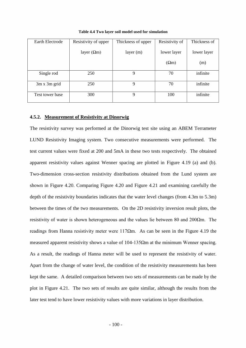
- 100 -
Table 4.4 Two layer soil model used for simulation
Earth Electrode Resistivity of upper
layer (Ωm)
Thickness of upper
layer (m)
Resistivity of
lower layer
(Ωm)
Thickness of
lower layer
(m)
Single rod 250 9 70 infinite
3m x 3m grid 250 9 70 infinite
Test tower base 300 9 100 infinite
4.5.2. Measurement of Resistivity at Dinorwig
The resistivity survey was performed at the Dinorwig test site using an ABEM Terrameter
LUND Resistivity Imaging system. Two consecutive measurements were performed. The
test current values were fixed at 200 and 5mA in these two tests respectively. The obtained
apparent resistivity values against Wenner spacing are plotted in Figure 4.19 (a) and (b).
Two-dimension cross-section resistivity distributions obtained from the Lund system are
shown in Figure 4.20. Comparing Figure 4.20 and Figure 4.21 and examining carefully the
depth of the resistivity boundaries indicates that the water level changes (from 4.3m to 5.3m)
between the times of the two measurements. On the 2D resistivity inversion result plots, the
resistivity of water is shown heterogeneous and the values lie between 80 and 200Ωm. The
readings from Hanna resistivity meter were 117Ωm. As can be seen in the Figure 4.19 the
measured apparent resistivity shows a value of 104-135Ωm at the minimum Wenner spacing.
As a result, the readings of Hanna meter will be used to represent the resistivity of water.
Apart from the change of water level, the condition of the resistivity measurements has been
kept the same. A detailed comparison between two sets of measurements can be made by the
plot in Figure 4.21. The two sets of results are quite similar, although the results from the
later test tend to have lower resistivity values with more variations in layer distribution.

- 101 -
(a) Measurement at 200mA
(b) Measurement at 5mA
Figure 4.19 Measured apparent resistivity against Wenner spacing
Ap
p. r
esis
tivi
ty
(Ωm
)
Wenner spacing a (m)
rho(max)
rho(av)
rho(min)
Ap
p.
resi
stiv
ity
(Ω
m)
Wenner spacing a (m)
rho(max)
rho(av)
rho(min)

- 102 -
(a) Measurement at 200mA
Based on the results of the water resistivity survey, Dinorwig test site was represented as two
layer model as shown in Table 4.5.
Table 4.5 Resistivity model of Dinorwig test site
Depth of layer (m) Resistivity (Ωm)
5.5 115
Infinite 600
These resistivity values were subsequently used for CDEGS simulation purposes by
substituting the actual depth of low resistivity water level at the time of measurements of test
electrodes: Rod 2A (Rod having dimensions 14mm diameter and 96cm immersed in water)
and 5m x 5m grid. Unlike the Llanrumney test site, there is relative ease of the representation
of the resistivity of the conducting medium in the form of horizontally layered model for
Dinorwig test site. The measured resistivity pattern of Dinorwig test site is shown in Figure

- 103 -
4.21. As seen from the inverse model resistivity section of the figure (lower part of Figure
4.21), the upper layer of water (up to about 5m depth) is of fairly uniform resistivity close to
100Ωm. The water level measured at the start of the resistivity measurement was 3.7m. The
resistivity of the bottom layer is gradually becoming higher. The bottom of the lake at the
Dinorwig test site is rocky. The seepage of water through the porous rock may be the cause of
the gradual increase in the resistivity of the lake bottom below 5m depth.
(b) Measurement at 5mA
Figure 4.20 Two dimension resistivity distributions

- 104 -
Figure 4.21 Resistivity of lake bed in two measurements
4.6. Summary
As described in this chapter Llanrumney test site has various practical earthing systems such
as single rod, cluster of rods, horizontal electrode, ring earthing system, 3m x 3m grid, test
tower base and National Grid 275kV operational tower base VP9. The soil resistivity
measurements at Llanrumney test site have shown that there is considerable variation in soil
resistivity both according to the position in the field and also with depth. Furthermore it has
also been observed that the significant seasonal variations in soil resistivity occur.
The Dinorwig test site had a scope of testing the practical earthing systems such as single rod,
horizontal electrode and 5m x 5m earthing grid in the relatively uniform medium as lake
water of the pumped hydro power station. The water resistivity measurements conducted at
various locations of the lower lake Lynn Peris of the Dinorwig pumped hydro power station
indicated that the water resistivity is fairly uniform over a given day. There are some seasonal
variations in the resistivity of water which may be attributed to the difference in
temperatures.

- 105 -
Cardiff University Impedance Measurement System (IMS), Radio Frequency System,
Impulse Current Injection System and ABEM Terrameter soil resistivity systems were also
introduced in this chapter.

- 106 -
Chapter 5: Characterisation of earth electrodes under variable
frequency and impulse energisation using full scale field tests
The earth resistance/impedance of operational power system installations is normally
measured using test equipment generating low injection current magnitudes [11] [31]. For
earth impedance measurements, a sinusoidal signal is injected into the earth electrode and by
measuring the earth potential rise at the point of injection, the earth impedance is calculated
by taking the ratio of the measured voltage to injected current. Such ac tests are normally
performed at frequencies away from the power frequency [8] [24] [25] [32]. Many
commercial ‘composite’ earth testers are available and these use a variable frequency
switched DC energisation and measure the test electrode earth resistance [24]. Previous work
[32] has indicated that quite different values of earth resistance/impedance are obtained when
using test equipment producing different current magnitude, wave shape and frequency.
The high frequency behaviour of earthing systems is of interest in applications where high
frequency currents are to be effectively dissipated in the earth, such as lightning currents or
transient surges. The earthing systems are also expected to keep the step, touch and
transferred earth potentials within the limits specified by the standards [11] [31]. If the safety
voltages and transferred earth potential magnitudes are within the specified limits, it provides
human safety as well as protection to the neighbouring communication circuits during
lightning faults, transient faults and power frequency fault conditions on the electrical power
systems.
The staged fault test employs a test current injection of magnitude similar to the fault current
level into the earthing system under test and then measuring the resulting earth potential rise
(EPR). The ratio of the RMS value of the Earth Potential Rise (EPR) to the RMS value of the
injected current gives the value of earth impedance. This method is rarely used [16] due to
two main drawbacks;

- 107 -
a) It involves disconnecting the earthing system from the circuit which it is protecting, which
may in turn result in the protected system to be cut off from power supply for the duration of
testing.
b) The injection of high current levels similar to the fault current magnitudes is not
economical particularly if the earthing systems to be tested are large such as substation
earthing systems, where the magnitudes of fault currents are high.
Other methods of measuring earth impedance involve the use of relatively smaller
magnitudes of sinusoidal test currents at different frequencies of interest. The ratio of RMS
value of resulting earth potential rise to the RMS value of injected current gives the value of
measured earth impedance of the system. Some instruments use impulse signals to test the
earth impedance. The ratio of the FFT (Fast Fourier Transform) of the resulting EPR impulse
signal to the FFT of the injected current impulse signal will give the values of measured earth
impedance in frequency domain [33] [43].
In order to measure the earthing impedance at variable frequency and current magnitudes, a
series of earth tests were performed at the Cardiff University test site in Llanrumney and at
the Dinorwig Power station test site (lower lake Lynn Peris). The test results were obtained
with different energisation sources such as switched DC/variable frequency, AC/variable
current AC/low voltage impulse. Tests were carried out on earthing systems including an
operational 275kV transmission tower VP9, the test tower base, a small grid (3m x 3m size),
single earth rod, ring earthing, cluster of rods and various Dinorwig test setups. The measured
voltages and currents together with calculated impedance / resistance values are presented
here.
5.1. Tests on single earth rod at Llanrumney test site
5.1.1. Earth resistance / impedance tests on single earth rod

- 108 -
Figure 5.1 shows the test set up for measuring the earth impedance of a single rod with the
Cardiff University Impedance Measurement System (IMS) [32]. The test object was a single
copper rod (Rod 1 of ring earthing system shown in Figure 5.1) with a 16 mm diameter and
buried at 2.4m depth. The test current was injected in the test object (single earth rod) and the
return current was extracted from the test tower base (shown in Figure 5.1), which was 30m
away from the test object. The earth potential rise at the point of current injection in the test
object was measured with respect to a remote reference electrode, as shown in Figure 5.1
which was placed at a distance of 100m from the test object and at 90 to the return current
lead. The test sources were fed from a 240V A.C. power supply via an isolation transformer.
Figure 5.1 Test set-up for measurement of earth impedance of single earth rod
The measured values of the rod earth impedance at different frequencies obtained using the
IMS are shown in Figure 5.2. The earth impedance of a single rod was measured at varying
current magnitudes (few tens of mA to few amperes) although for these initial tests, the
current was not kept constant over the entire frequency range. At any given current
- 109 -
magnitude, there is a reduction of about 10% in the measured earth impedance of a single rod
over the frequency range from 20Hz to 100kHz. It is to be noted that the phase angle of the
measured earth impedance of single earth rod was observed to be less than 5° and capacitive
in nature. This small capacitance effect will result into marginal decrease of the measured
earth impedance. However, the reduction in the measured earth impedance of 10% is found to
be a decrease in the resistive nature, which can be explained by the following statement. It
was calculated that, in order for the capacitive effect to result in the reduction of 10%
impedance, the phase angle should have been more than 30°.
In addition at low frequencies (< 100Hz), there is a pronounced frequency effect for currents
lower than 50mA. This finding has important implications for low current test systems. All
the curves tend to converge at the same point at a frequency of around 100 kHz. It is to be
noted that the IMS (Impedance Measurement System) filters the noise in the measured EPR
signal with the help of a suitable filter. The current was measured with the help of a LILCO
CT with an output of 0.1V/A. The minimum current measured was 13.6mA. At the minimum
measured current during this experiment it provided a voltage output of 1.36mV. It is to be
noted that the IMS system has a resolution to measure accurately the single level of few
hundred microvolts.

- 110 -
50
52
54
56
58
60
62
10 100 1000 10000 100000Frequency (Hz)
Imp
ed
an
ce
(Ω
)13.6mA to 15.6mA
26.3mA to 29.4mA
40.4mA to 45.4mA
890mA to 1806mA
452mA to 1179mA
99.3mA to 112.1mA
Figure 5.2 Earth impedance tests with IMS on a single 2.4m earth rod
Figure 5.3 shows the variation of earth impedance with current for the same set of test results.
As can be seen from the figure the effect of current on earth resistance / impedance is more
significant at low frequency e.g. when the measurement is performed with the ABEM
Terrameter (switched DC frequency of 0.5Hz) and using the IMS at 20Hz. Figure 5.3 also
shows the earth resistance of the single earth rod measured with the DET 2/2 (switched DC
frequency of 128Hz). The earth impedance at frequencies above 100Hz have negligible
variation with current. The effect of current magnitude on the impulse resistance is also
shown in the figure. The impulse earth resistance was calculated from the ratio of the impulse
earth potential rise at the instant of peak impulse current and the peak value of the impulse
current waveform. It was observed that the peaks of the earth potential rise and the current
waveforms occurred almost at the same instant for slow (rise time greater than few hundreds
of µs) and fast (rise time of few µs) impulse waveforms for the single earth rod as shown in
Figure 5.4 and Figure 5.5 respectively.

- 111 -
50
52
54
56
58
60
62
64
66
68
70
72
0.001 0.01 0.1 1 10
Current (A)
Resis
tance /
Im
pedance (
Ω)
ABEM (DC)
DET 2/2
Impulse resistance
20Hz AC
10kHz AC
40kHz AC100kHz AC
Figure 5.3 Variation of impedance with current
5.1.2. Low Voltage Impulse Tests on Single Earth Rod
Slow and fast low voltage impulse tests were performed on the single earth rod to investigate
the behaviour of the earth impedance under various impulse conditions. Typical results of the
injected current and the measured earth potential rise for the slow and fast impulse tests are
shown in Figure 5.4 and Figure 5.5 respectively. The peak values of the injected current and
the earth potential rise recorded during the low voltage impulse tests are also shown in Figure
5.4 and Figure 5.5. The Fast Fourier transformed response of the impulse tests is shown in
Figure 5.6. As can be seen from the figure, the earth impedance is seen to be decreasing as

- 112 -
the frequency content in the impulse signal increases. Comparing Figure 5.2 and Figure 5.6
we can infer that the response of single earth rod to the variable frequency tests closely
resembles to that of the response of the single earth rod to the low voltage impulse tests.
Figure 5.4 Low voltage impulse (LVI1) test waveforms

- 113 -
Figure 5.5 Low voltage impulse (LVI2_B) test waveforms
0
10
20
30
40
50
1 10 100 1000 10000 100000 1000000
Frequency (Hz)
Freq. scan
FFT
Ea
rth
im
pe
da
nce
(Ω
)
Figure 5.6 Comparison of FFT of impulse waveforms and frequency scan of earth impedance for single
rod

- 114 -
5.2. Tests on single earth rod at Dinorwig test site
Figure 5.7 shows the set up for testing a single earth rod at Dinorwig test site. As can be seen
in the figure, the test rod electrode was located at the end of the pontoon. A potential
reference electrode with a floating lead was placed 70m away and perpendicular to the
pontoon. The current return electrode was immersed in the lake towards the shore-end of the
float system. The test electrode comprised a single copper earth rod, 14mm in diameter and
1.2m long. The top end of the rod was fixed to the end section of the floating pontoon in a
vertical orientation. The length of the test rod immersed in water was 0.8m. A single rod,
0.15m long and 9mm in diameter, was used for the ‘90˚’ potential reference electrode. A 5m
long aluminium tape, 50mm×6mm, 0.6m below water surface, was used as the current return
electrode.
Figure 5.7 Plan view of test set up for testing single rod at Dinorwig test site

- 115 -
In previous preliminary tests [43], the voltage sources were located in the test cabin and the
test electrode was energised using a transmission line located along the pontoon. However,
for this particular series of tests, the voltage sources and measuring instruments were located
in the boat adjacent to the test electrode. This arrangement was chosen in order to minimise
the effects of coupling between the test leads. The test sources and instrumentation were fed
from a low-voltage supply installed along the pontoon via an isolation transformer. A short
lead from the boat to the pontoon was used to inject current from the source into the test
object. The current return electrode placed in the water at the shore-end of the pontoon was
connected back to the source using an insulated line laid along the pontoon. An additional
lead was used to obtain potential measurements between the test electrode and the ‘90˚’
reference electrode. Optically-isolated differential voltage probes and current probes were
used for voltage and current measurements respectively. The voltage sources comprised; i)
two DC sources: a ‘composite’ commercial earth resistance tester (DET 2/2) and a geo-
physical resistance meter (ABEM Terrameter), (ii) two AC sources: a variable AF impedance
measurement system (IMS) [42], an RF measurement system, and (iii) a HAEFELY recurrent
surge generator.
A DC resistance of 117.6Ω was measured using the ‘composite’ tester and 118.2Ω was
obtained with the geo-physics earth tester at its highest current setting of 500mA. The
calculated ‘earth’ resistance of the rod using Equation (5.1) [1] is 95.4Ω, assuming a water
resistivity measured at 93.5Ωm.
(5.1)
The ‘earth’ resistance calculated using a commercial earthing software (CDEGS) [67] is
100.3Ω, based on a simplified two-layer medium with a 9m upper-layer of 93.5Ωm, εr=80

- 116 -
(water) and a lower layer of about 600Ωm, εr=1 (lake bed rock). Using the same software,
with the electrode modelled in a single-layer medium having the properties of the water, a
resistance of 98.2Ω is calculated.
It was observed that the measured resistance changes with current magnitude. Figure 5.8
shows the reduction in earth resistance over the range 1mA to 500mA for DC tests using the
geo-physics meter. Although current dependence of earth impedance has been studied
previously, the focus has been on soil ionisation phenomena at very high current magnitudes.
Current dependence of earth resistance at pre-ionisation levels was reported in [14] in the
range 130 to 1300A. However, commercial earth testers usually operate at current
magnitudes below 10A and some instruments generate currents as low as of the order of
100mA. These results suggest that low current magnitude tests may over-estimate the earth
resistance of electrodes compared with the resistance seen at higher current magnitudes of the
levels seen under the fault conditions.
Figure 5.8 Effect of current magnitude on measured earth resistance
110
114
118
122
126
130
0.001 0.010 0.100 1.000
Re
sis
tan
ce
(Ω
)
Current (A)
Rod 2 (ABEM)

- 117 -
5.2.1. Rod ‘earth’ impedance
Using the same test setup as for the earth resistance tests, the ‘earth’ impedance of the rod
was measured using the IMS system. At 50Hz, the measured value was 122.2 with a
current injection of 400mA. For this particular electrode, the value is close to the measured
DC ‘earth’ resistance. The comparison of the measured impedance of the single earth rod at
50Hz with the DC earth resistance and the calculated / simulated values of earth rod
impedance is shown in the Table 5.1.
Table 5.1 Comparison of measured earth resistance / impedance with analytical impedance
Test object: Single rod 14mm Ø, 80cm immersed in water Resistance / Impedance
DC resistance measured with DET 2/2 117.6Ω
DC resistance measured with ABEM 118.2Ω @ 500mA
Impedance @ 50 Hz 122.2Ω @ 400mA
Calculated value of impedance 95.4Ω
Simulated value of impedance with CDEGS software 100.3Ω
As can be seen from the table, the measured earth resistance / impedance at 50Hz are in fair
agreement. However, the analytical calculations show lesser value of the impedance. This
could be attributed to the constraint in accurately estimating the lower layer rock bed
resistivity. The simulation results are further discussed in Chapter 6.
5.2.2. Variable frequency earth impedance measurement
The AC tests were extended to determine the earth impedance over the frequency range 20Hz
to 10MHz and the results are plotted in Figure 5.9. The IMS system was used to test over the
range 20Hz to 40kHz and the source was maintained at a constant current magnitude of
400mA throughout, to eliminate the effect of current magnitude on impedance. The RF
system was employed above 30kHz. As can be seen in Figure 5.9, there is a close overlap in

- 118 -
the results for the common frequencies tested by both systems (IMS and RF) for a frequency
range 30kHz to 40kHz.
Using a lumped-parameter circuit model for a rod-type electrode, as shown in Figure 5.9, the
frequency response of the system was calculated using P-SPICE. The calculated values of R,
L, and C are shown in Figure 5.10 using the previously defined geometric dimensions of the
rod (14mm Ø, 80cm immersed in water) and the water resistivity and permittivity (ρ=93.5Ωm
and εr=80). R, L and C for the vertical rod were calculated using equations (5.2), (5.3) and
(5.4) given by [68]
------ (5.2)
------ (5.3)
------ (5.4)
The calculated frequency response of the rod obtained from the circuit model is also shown in
Figure 5.9 together with values calculated using the CDEGS model with the 2-layer model
(9m upper-layer of 93.5Ωm, εr=80 (water) and a lower layer of about 600Ωm, εr=1 (lake bed
rock)).

- 119 -
Figure 5.9 Plots of measured and simulated earth impedance magnitude with frequency
As can be seen in Figure 5.9, the overall shape of the three curves (one measured and two
simulated) is similar. The shape of the curves is characterised by a relatively flat region of
impedance from low frequency up to the region of 200Hz to 500kHz. Over this lower
frequency range, the measured earth impedance (resistance) is about 20% higher than the
simulated values. However, in the frequency range 20Hz to 40kHz, there is an indication of a
reduction in measured impedance that is not predicted using the conventional earthing system
model that assumes constant resistivity and relative permittivity. Above the 500kHz
frequency, the measured earth impedance falls rapidly. This trend is also observed with the
simulation models which may indicate an increasing capacitive effect.
0
20
40
60
80
100
120
140
1.E+01 1.E+02 1.E+03 1.E+04 1.E+05 1.E+06 1.E+07 1.E+08
Impedance (
Ω)
.
Frequency (Hz)
Circuit model simulation
CDEGSsimulation
Measurement

- 120 -
Figure 5.10 Lumped parameter circuit model for a rod electrode
5.2.3. Low voltage impulse tests
Low voltage impulse tests with different magnitudes and impulse shapes were carried out on
the test rod. The transient ‘earth’ potential rise of the rod was measured with respect to the
‘90°’ reference electrode for a 20/80 current impulse, and the results are shown in Figure
5.11. From the figure, it can be seen that the voltage peak occurs at the same time as the
current peak for this electrode and impulse shape, indicating a mainly resistive behaviour.
The parametric details of the voltage and current impulse recordings are shown in Table 5.2.
With the voltage and current traces in phase, the impulse resistance was calculated as 118.1
by dividing the peak voltage by peak current. This impulse resistance value is very close to
the measured resistance values using the DC earth testers as shown earlier in Table 5.1.
The results of water resistivity measurements at the reservoir (as discussed in section 4.2)
confirm that the water resistivity and temperature on any given day is largely uniform, both
depth-wise and area-wise. However, seasonal variations are evident. Figure 5.12 and Figure
5.13 show the variation of measured earth impedance of various single earth rods (Rod 2:
14mm Ø, 80cm immersed in water, Rod 2A: 14mm Ø, 96cm immersed in water and Rod 3:
14mm Ø, 200cm immersed in water) with frequency and current magnitude of the injected
current.

- 121 -
Figure 5.11 Low voltage impulse test results on a 0.8m rod
Table 5.2 Parameters of the impulse waveforms
Wave shape of current trace Impulse rise time Impulse fall time
18.92μs 82.71μs
Current (A) 0.082
EPR (V) 9.68
R (Ω) 118.1
5.2.4. Effect of current magnitude on measured earth impedance of signle rod at
Dinorwig
The effect of current magnitude on the measured earth impedance is pronounced for the DC
and low frequency AC energisation experiments conducted at Dinorwig test site. It was
observed that the earth impedance of a single rod showed a reduction of about 10% with
increase in frequency (over the range 20Hz to 100kHz) when the measurement was
performed with the injection source placed next to the test object for the case of Rod 2 shown
in Figure 5.13.
-100 0 100 200 300 400 500-1
0
1
2
3
4
5
6
7
8
9
1020080807_Dinorwig_80cm Rod in Water LVI3A1_aver00000
Time (s)
Voltage (
V)
-0.01
0
0.01
0.02
0.03
0.04
0.05
0.06
0.07
0.08
0.09
0.1
Curr
ent (A
)
EPR .
Current
EPR
Current

- 122 -
Figure 5.12 Effect of current magnitude on earth impedance of single rod at Dinorwig test site
Figure 5.13 Effect of frequency on earth impedance of single rod at Dinorwig test site
As can be seen from Figure 5.12, the effect of DC current is more pronounced on the
measured earth impedance when the measurement is performed with ABEM Terrameter as
compared to that performed by the DET 2/2. In the case of ABEM Terrameter, the current is

- 123 -
varied from 1mA to 500mA while the DET 2/2 injects 7mA and 50mA DC currents at low
and high settings of the current.
5.3. Tests on 3m x 3m grid at Llanrumney test site
Figure 5.14 shows the test set up for the experiments on the 3m x 3m earth grid at the
Llanrumney test site. DC / Variable frequency AC / variable current AC / low voltage
impulse injection tests were performed on the 3m x 3m earth grid. The test current was
injected into the 3m x 3m grid and the return current was collected from the Test Tower Base
(TTB) which is 43m away from the 3m x 3m grid.
Figure 5.14 Experimental setup for tests on 3m x3m grid at Llanrumney test site
The variable current test results are shown in Figure 5.15. The effect of current magnitude on
measured earth impedance was investigated by varying test current in both ascending and
descending order. The test results indicate that the direction of change in current magnitudes
does not have any significant effect on the trend. It was also observed that, the effect of
current magnitude on earth impedance is more pronounced at lower frequencies and that, as

- 124 -
the frequency of injected current increases, the grid response in terms of earth impedance to
injected current tends to become flat. It should be noted that the similar effect of current was
observed on the measured earth impedance of the single earth rod as shown in Figure 5.3,
where it is shown that the effect of current is more pronounced at DC and low frequencies
and that, as the frequency increases, the effect of current tends to reduce.
9.0
10.0
11.0
12.0
13.0
14.0
15.0
0.001 0.01 0.1 1 10
Current (A)
ABEM
80kHz30kHz
Impulse5μs risetime
10kHz
1kHz100Hz
20 Hz
DET 2/2 - (12.28Ω)
52 Hz
Impedance (
Ω)
Figure 5.15 Effect of current on earth impedance of 3m x 3m grid
Figure 5.17 shows the variation of earth impedance with a variable frequency test and when
computed from the FFT of measured impulse current and EPR signals shown in Figure 5.16.
For the frequency scan part of the experiment, for investigation of the effect of frequency on
the measured earth impedance, the frequency of the injected current signal was varied from
20 Hz to 100kHz. In other part of the experiment, the impulse current was injected and the
EPR signal was acquired. The impulse current and EPR signals were captured with a Lecroy

- 125 -
waverunner 64Xi oscilloscope. The sampling interval was 200 ns and the sampling depth was
100 ksamples. The time for which the signal was acquired was 200 ns x 100 ksamples = 10
ms. So, the lowest frequency obtained in the computed FFT results is 1/10 ms = 100 Hz and
the FFT plot is in 100 Hz steps up to the highest frequency component of the impulse current
signal. The rise time of the impulse current signal was 8 μs. The results from this analysis
show a reduction of 15% in the magnitude of the earth impedance with frequency (100Hz to
30kHz). The FFT analysis of the impulse tests results, shown in Figure 5.16, gives a similar
trend of reduction of measured earth impedance with frequency increase as that obtained with
the variable frequency test on the 3m x 3m earth grid. It should be noted that the measured
earth impedance with frequency scan and that computed from the FFT from impulse signals
show close agreement over the range 100Hz to 60kHz.
Figure 5.16 Impulse waveforms

- 126 -
Figure 5.17 Variation of impedance with frequency scan and that computed from the FFT of impulse
5.4. Tests on 5m x 5m grid at Dinorwig test site
The plan view of the test set up for measuring the impedance of the 5m x 5m grids and the
horizontal electrode 5m and 15m long is shown in Figure 5.18 (Please refer to Table 4.3
showing details of the various test electrodes used at Dinorwig test site).
5.4.1 Tests on the electrode Grid 1
The first grid (Grid 1) measures 5m5m and comprises 25 equal meshes (each measured
1m1m). The grid is made up of 12 pieces of aluminium strip, and each strip measures
5m50mm6mm. The grid was suspended from a specially constructed floating structure
and was positioned 0.2m below water surface. Grid 2 is dimensionally the same as Grid 1 but
positioned 0.4m below water surface. Figure 5.18 shows the test setup for the measurement
of the earth impedance of Grid 1. The injection sources were placed in the boat next to the
test object. The frequency dependence of earth impedance of Grid 1 was measured with the
‘IMS’ and ‘RF’ system. Figure 5.19 shows the effect of 20Hz AC and 52Hz AC current
magnitude on the measured earth impedance of Grid 1. As can be seen from Figure 5.21, the
- 127 -
impedance is flat up to about 50 kHz for Grid 1 and 100 kHz for Grid 2 and increases
significantly with frequency beyond this value.
5.4.2 DC earth resistance of Grid 1
The DC earth resistance was measured using DET2/2 (10.46Ω at low current setting and
10.44Ω at high current setting) and DET 4TC (10.53Ω for both 25V and 50V settings).
5.4.3 Current magnitude dependence of the impedance of Grid 1
The current magnitude dependence of the earth impedance was measured at 52Hz using the
IMS and the results are shown in Figure 5.19. Comparing Figure 5.19 with Figure 5.12 and
Figure 5.15, it can be said that a similar trend of the effect of current magnitude on the
measured earth impedances is found for the 5m x 5m grid, 3m x 3m grid and the single earth
rod. Figure 5.20 shows the current dependence of earth resistance of Grid 1 when measured
with the geophysical meter (ABEM Terrameter). As can be observed from the figure, the
variation of impedance with current is more pronounced at DC currents less than 10mA.
5.4.4 Low voltage impulse tests on Grid 1
Figure 5.22 shows the comparison between the measured impedance with the impedance
computed with the FFT-based on one low voltage impulse test. The ‘FFT’ method produces
values very close to the results obtained from the swept-frequency AC tests.
5.4.5 Tests on the electrode Grid 2
The same grid (i.e. Grid 1) was lowered to 0.4m below water surface and was tested. The
new configuration is referred to as ‘Grid 2’. The swept frequency response of the impedance
of Grid 2 is also shown in Figure 5.21 (designated as curve C). The measured earth

- 128 -
impedance of Grid 2 is lower than the measured earth impedance of Grid 1 as the depth of
Grid 2 is larger than the Grid1. There is negligible effect of frequency on the measured earth
impedance for Grid 1 and Grid 2 over the frequency range 20Hz to 10kHz and 20Hz to
50kHz respectively. The measured earth impedance of Grid 1 and Grid 2 increases sharply
above the frequency of 100kHz. DC earth resistance was measured by DET2/2 (9.26Ω at low
current setting and 9.27Ω at high current setting) and DET 4TC (9.51Ωfor both 25V and 50V
settings).
Figure 5.18 Plan view of test set up for testing 5m x 5m earth grid and horizontal electrode at Dinorwig

- 129 -
Figure 5.19 Current dependence of earth impedance of a Grid 1 at 20Hz and 52Hz
Figure 5.20 Current dependence of earth impedance of a Grid 1 at DC current (ABEM)

- 130 -
Figure 5.21 Effect of frequency on earth impedance of 5m x 5m grid at Dinorwig test site
Figure 5.22 Comparison of Swept frequency and FFT from impulse methods of measurement of earth
impedance of 5m x 5m earth grid.

- 131 -
5.5. Tests on the horizontal electrode
A horizontal electrode of dimensions 5mx50mmx6mm suspended at 0.20m below water
surface is referred to as Horizontal Electrode 1. A horizontal electrode, made up of 3 pieces
of 5m50mm6mm aluminium strips and suspended at 0.25m below water surface is referred
to as Horizontal Electrode 2. The injection and measurement point was at the centre of the
horizontal electrodes. The test set up for measurement of impedance of horizontal electrodes
is shown in Figure 5.18. The results of the swept frequency on the horizontal electrode are
shown in Figure 5.23. As can be seen from Figure 5.23, the earth impedance is marginally
falling with frequency up to a frequency of around 100 kHz. Above 100kHz, an increasing
trend of earth electrode impedance with increase in frequency can be seen for the Horizontal
Electrode 1.
Figure 5.23 Effect of frequency on earth impedance of horizontal electrode at Dinorwig test site

- 132 -
5.5.1 DC earth resistance of Horizontal Electrode 2
The DC earth resistance of Horizontal Electrode 2 was measured using the DET2/2 (14.63Ω
at low current setting and 14.62Ω at high current setting) and the DET 4TC (14.57 and
14.59Ω for 25V and 50V settings respectively).
5.5.2 The current magnitude dependence of impedance of Horizontal Electrode 2
Figure 5.24 shows the current magnitude dependence of earth impedance of Horizontal
Electrode 2 measured at 20Hz using the IMS. It can be seen that there is a small increase in
the measured earth impedance of the horizontal electrode with the increase in current
magnitude from few mA to about 5A. This trend is opposite to that observed for the other
electrodes tested during the field tests. It is shown in the Chapter 7.7 (Figure 7.10) that with
the current density in the range of 0.003A/m2 to 0.01A/m
2 the measured earth impedance
exhibited a rising trend with the increase in injected current magnitude. The current density in
the horizontal electrode is low as the area of horizontal electrode is sufficiently large. It is to
be noted that the low current injection into the grids / other electrodes with large surface area
will result in low current densities into the earthing electrode under test. It is believed that
this condition will tend to exhibit increasing trend in the measured earth resistance with the
increase in the current magnitude.

- 133 -
Figure 5.24 Current magnitude dependence of earth impedance of a horizontal electrode
5.6. Tower base tests at Llanrumney
5.6.1. Purpose built test Tower base (TTB)
With a low voltage variable frequency AC applied to the test tower base (TTB), its earth
impedance was measured. DC and impulse tests were also conducted on the same electrode.
The test setup is shown in Figure 5.25. It was observed that the earth impedance decreased
with increase in frequency as shown in Figure 5.26. This trend was also seen from tests on
the small grid and the other test electrodes at Llanrumney. The tests carried out on the single
rod immersed in the lake at Dinorwig also showed a similar trend.
An AC test with current varying from 10mA to 2.5A was also performed on the same day,
and as can be seen from Figure 5.27, the measured earth impedance decreased by about 7% at
different tested frequencies. The reduction in earth impedance of test tower base with
increase in current magnitude was most prominent of all the electrodes tested so far. Figure
5.27 also shows that the reduction of earth impedance with current is observed above a
current magnitude of 100mA for the AC tests. The values of impulse resistance (EPR peak
Imp
ed
ance m
ag
nitu
de
(Ω
)
Current (A)
20 Hz

- 134 -
divided by injected current peak) are also shown in Figure 5.27 together with selected results
from the DC and variable frequency AC tests. (Note that the peaks of voltage and current in
these tests occurred at the same time). From the figure, it can be observed that the earth
resistance values from the impulse tests lie between the earth impedance values obtained at
10kHz and 60kHz respectively from the variable frequency tests.
Figure 5.25 Set up for measuring earth impedance of test tower base at Llanrumney
The impulse signals with rise times of 5.1µs and 2.2µs also show a similar trend of reduction
of measured earth resistance with increase in the current magnitude. It should be noted that
the relatively lower frequency components are present in the 5.1µs rise time signals
compared with the 2.2µs rise time signals. Hence, the measured earth resistance with 5.1µs
rise time signals is greater than that measured with the 2.2µs rise time signals.

- 135 -
18
19
20
21
22
23
24
10 100 1000 10000 100000Frequency (Hz)
Z(102.0mA to 130.9mA) Z(644mA to 702mA) Z(949mA to 1057mA)
Z(1308mA to 1388mA) Z(1634mA to 1736mA) Z(2099mA to 2153mA)
Z(2502mA to 2665mA) Z(3165mA to 3377mA) Z(4213mA to 4444mA)Im
pe
da
nce
(Ω
)
Figure 5.26 Effect of frequency on tower earth impedance tested at Llarumney
Figure 5.27 Effect of current on tower earth impedance tested at Llanrumeny
17
19
21
23
25
27
0.001 0.01 0.1 1 10Current (A)
ABEM (DC)
52Hz
60kHz
50kHz
10kHz
5kHz
100Hz
Impulse (Tr = 5.1μs)
Impulse (Tr = 2.2μs)
Imp
ed
an
ce
(Ω
)

- 136 -
5.6.2. Operational tower (VP9) tests
Variable frequency tests were performed on the earthing system of the National Grid 275 kV
operational transmission tower (VP9) at Llanrumney test site. The tests carried out on 2nd
and
12th
June 2008 were made with the overhead earth wire (OEW) connected. Variable
frequency current was injected in one of the leg of VP9 tower base, and the isolated tower
base was used as current return. Further tests were carried to investigate the effect of
disconnecting the earth wire from tower VP9 using a purposely installed pneumatic switch.
Figure 5.28 shows the variation of measured earth impedance with the frequency during these
tests. The measured impedance of the 275kV transmission tower represents the parallel
summation of the chain impedances on both sides of VP9 and the earth impedance of the
individual tower. As the frequency is increased, the earth impedance increases and tends
towards a constant value of about 11.5 above 30 kHz.
With the overhead earth wire (OEW) disconnected, the measured earth impedance of VP9
tower is about 15 at low frequencies (20 Hz to 40 Hz). As the test frequency increases, the
magnitude of impedance reduces. At higher frequencies, (>2 kHz and up to 70kHz ) the
measured earth impedance of VP9 tower is close to 12Ω. With the overhead earth wire
connected, the measured earth impedance of VP9 tower is about 0.2 at low frequencies (20
Hz to 40 Hz). The low value of measured earth impedance of VP9 tower at frequencies
(20Hz to 40Hz) is due to the parallel summation of the chain impedances of the operational
National Grid towers on both sides of VP9. As the test frequency increases, the magnitude of
impedance increases up to about 11Ω over the frequency range 30kHz to 70kHz. The
increase in impedance is the result of inductive effects at higher frequencies. It should be
noted that the measured earth impedance of the VP9 tower at higher frequencies is in close
agreement for both cases of overhead earth: wire connected and disconnected. Figure 5.28
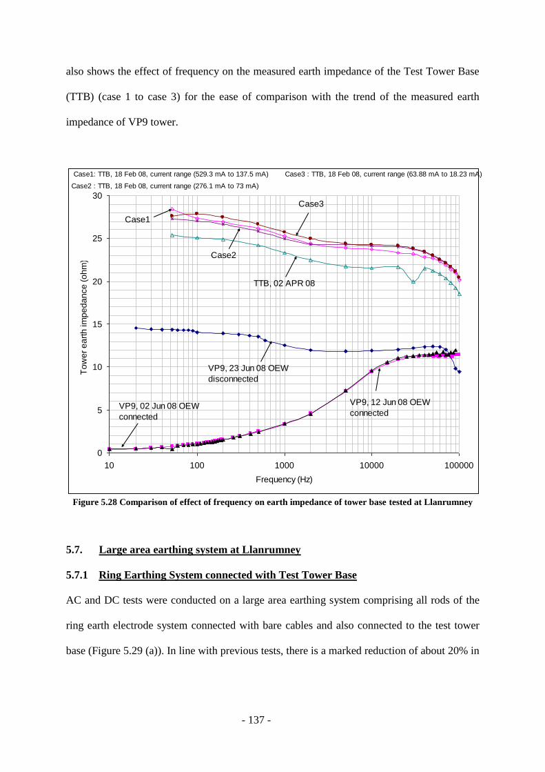
- 137 -
also shows the effect of frequency on the measured earth impedance of the Test Tower Base
(TTB) (case 1 to case 3) for the ease of comparison with the trend of the measured earth
impedance of VP9 tower.
Figure 5.28 Comparison of effect of frequency on earth impedance of tower base tested at Llanrumney
5.7. Large area earthing system at Llanrumney
5.7.1 Ring Earthing System connected with Test Tower Base
AC and DC tests were conducted on a large area earthing system comprising all rods of the
ring earth electrode system connected with bare cables and also connected to the test tower
base (Figure 5.29 (a)). In line with previous tests, there is a marked reduction of about 20% in
0
5
10
15
20
25
30
10 100 1000 10000 100000
Frequency (Hz)
To
we
r e
art
h im
pe
da
nce
(o
hm
)
VP9, 12 Jun 08 OEW
connectedVP9, 02 Jun 08 OEW
connected
VP9, 23 Jun 08 OEW
disconnected
TTB, 02 APR 08
Case2
Case1
Case3
Case1: TTB, 18 Feb 08, current range (529.3 mA to 137.5 mA)
Case2 : TTB, 18 Feb 08, current range (276.1 mA to 73 mA)
Case3 : TTB, 18 Feb 08, current range (63.88 mA to 18.23 mA)

- 138 -
measured DC resistance (ABEM meter) over the range 1mA to 1A and an 8% reduction in
measured AC impedance at 20Hz over the range 200mA to 3A.
A decreasing trend in impedance with frequency was observed over the frequency range of
20Hz to 2kHz, as shown in Figure 5.29 (b). However, for this more extensive earth electrode,
the earth impedance rises sharply above 10kHz. A sharp rise in earth impedance was also
observed from tests on the extended tower earthing system at tower VP9, but in this case, the
upturn in earth impedance occurred at a much lower frequency which attributed to the greater
inductance of the tower line earthing system.
Figure 5.29 Effect of frequency on large area earthing system at Llanrumney

- 139 -
5.7.2 Cluster of Three Rods connected with Horizontal Electrode at Llanrumney
Variable frequency AC tests were carried out on a cluster of three rods connected with
horizontal electrode at the Llanrumney test site. The test set up is shown in Figure 5.30.
Figure 5.30 Test set up for Cluster of Three Rods with Horizontal Electrode
The test results are shown in Figure 5.31. As seen from the figure, the overall decreasing
trend of measured earth impedance is observed over the frequency range 20Hz to 100kHz.
Figure 5.31 Variation of impedance with frequency (Cluster of Three Rods with Horizontal Electrode)
0
2
4
6
8
10 100 1000 10000 100000
Ea
rth
im
pe
da
nce
(Ω
)
Frequency (Hz)

- 140 -
5.7.3 Cluster of Three Rods at Llanrumney
Variable frequency AC tests were carried out on a cluster of three rods at the Llanrumney test
site. The test set up is shown in Figure 5.32, and the test results are shown in Figure 5.33. The
overall decreasing trend of measured earth impedance observed over the frequency range
20Hz to 100kHz is similar to the other electrodes tested at Llanrumney and Dinorwig test
site.
Figure 5.32 Plan view of test set up (Cluster of Three Rods)
Figure 5.33 Variation of impedance with frequency (3 rod cluster)
10
12.5
15
17.5
20
10 100 1000 10000 100000 1000000
Frequency (Hz)
Ea
rth
im
pe
da
nce
(O
hm
)

- 141 -
5.8. Discussion of test results
5.8.1 Comparison of FFT from impulse and swept frequency results
The fast Fourier Transform of the impulse waveform provides the frequency spectrum of the
impulse waveform. The Fast Fourier Transforms of the measured injected current and earth
potential rise (EPR) signals were performed to obtain the magnitudes of these signals in the
frequency domain. The ratio of the EPR to injected current in the frequency domain provides
the earth impedance in the frequency domain. The so-obtained earth impedance in the
frequency domain was compared with the frequency scan measurements of the earth
impedance carried out with the Impedance Measurement System (IMS).
5.8.1.1. Effect of windowing functions on the FFT output of impulse waveforms
To study the effect of windowing function on the FFT output, the slow and fast impulse
waveforms were transformed using FFT function of Origin 7 waveform analysis software. It
was observed that the rectangular windowing function (which is the same as applying no
window function) gives the better results in our case as compared to the results of other
windowing functions. It was observed that the results obtained with the FFT processing
showed the reduction of impedance of earth electrodes with increase in applied frequency,
and the trend was similar to those observed in the field tests with the variable frequency scan
on the earth electrodes tested in the field. FFT analysis of the impulse waveform can be used
to obtain the measured earth impedance values at different frequencies. FFT analysis of the
impulse signal waveforms of injected current and earth potential rise to obtain earth
impedance values can save considerable amount of time and equipment costs as compared to
the frequency scan procedure in the field. The comparison of earth impedance values
obtained from the FFT outputs of the slow/fast impulse signal waveforms using different
windowing functions are shown in Figure 5.34 and Figure 5.35. It was observed that the

- 142 -
Welch windowing function for the slow impulse waveform and the rectangular windowing
function for the fast impulse waveform provided better results for the FFT analysis of the
impulse test results.
Figure 5.34 FFT of slow impulse waveform with different windowing functions
Figure 5.35 FFT of fast impulse waveform with different windowing functions (enlarged view)
40
44
48
52
56
60
10 100 1000 10000
Eart
h im
ped
an
ce o
f sin
gle
ro
d (
Ω)
Frequency (Hz)
Rectangular window
Hamming window
Hanning window
Blackman window
Welch window Slow waveform
50
52
54
56
58
60
100 1000 10000 100000
Eart
h im
pedance o
f sin
gle
rod (
Ω)
Frequency (Hz)
Rectangular window
Hanning window
Hamming window
Blackman window
Welch window
Fast waveform

- 143 -
5.8.1.2. Comparison of FFT of the results obtained at Llanrumney test site
The measured impulse signals of voltage and current obtained from the field tests on the test
earth electrodes at Llanrumney were analysed using FFT and to obtain earth impedance
values as a function of frequency. The FFT results are shown in Figure 5.36, together with
the results of the measured impedance values obtained with the University’s IMS system. For
the single rod, 3m x 3m grid and the test tower base, the results show reasonably close
agreement between the earth impedance obtained with the FFT analysis and the frequency
scan over a restricted frequency range. In the case of the operational tower base VP9, the FFT
results showed a significant variation about the values obtained from the frequency scan.
Preliminary FFT analysis of impulse test results show reasonable agreement with swept-
frequency earth impedance measurements over a restricted frequency range.
Figure 5.36 Comparison of measured earth impedance obtained from frequency scan with the earth
impedance computed from FFT of measured impulse signals

- 144 -
5.8.1.3. Comparison of FFT of the results obtained at Dinorwig test site
Further analysis of experimental results of Dinorwig tests (conducted in June 2009) was
carried out. The comparison of the results of swept frequency and FFT from impulse for Rod
2A and 5m x 5m grid are shown in Figure 5.37. As seen from the figure, there is a close
agreement between the results for Rod 2A and 5m x 5m grid except for some intermediate
frequencies above 1MHz and up to 7MHz in the case of 5m x 5m grid.
Figure 5.37 Comparison of AC steady state measurements with impulse
5.8.2 Frequency dependence of earth electrode impedance
The extensive tests carried out with variable frequency AC and impulse signals, on various
practical earth electrodes showed that, the measured earth impedance decreases with increase
in frequency over the range 20 Hz to 120kHz. The reduction of earth impedance with
frequency is larger with the electrodes embedded in the soil than the electrodes immersed in
water. The overall reduction in the measured earth impedance was in the range of 10% to
30% over the frequency range 20Hz to 120kHz. The phase difference angle between the
measured earth potential rise (EPR) and the injected current was less than 5° over the range
20Hz to 120kHz. It is therefore understood, that the measured earth impedance was

- 145 -
dominantly resistive in nature. The resistivity of the soil surrounding the earth electrodes was
found to be decreasing with the frequency of the injected current.
5.8.3 Dependence of earth electrode impedance on injected current magnitude
A series of tests conducted on the various practical earth electrodes with the variable current
AC/DC/impulse signals showed that there is an effect of the current magnitude on the
measured earth impedance of the earth electrodes. The effect of DC current was found to be
larger than the effect of AC/impulse current. Moreover, it was also observed that the effect of
AC current magnitude above the frequency of 100Hz is lesser than that at the frequencies
below 100Hz for the various earth electrodes. There was a reduction of up to 15% in
measured earth impedance of the various electrodes with the increase in DC current
magnitude from 1mA to 500mA. This aspect is worth noting as various commercially
available earth testers inject currents at current magnitudes close to few tens of mA.
5.8.4 Impulse response of earth electrode impedance
Various practical earth electrodes were tested with slow and fast impulse current signals to
determine the behaviour of earth electrodes with impulse currents. It was observed that the
FFT of impulse provided close agreement of impulse test results with the variable frequency
AC test results. This confirmed that there is a reduction of earth impedance with increase in
frequency over the range 20Hz to 120kHz. The impulse tests carried out with the variable
impulse current magnitudes also confirmed that the effect of increase in impulse current
magnitude is similar to the effect of current magnitudes at the corresponding high frequency
contents in the impulse signal.
5.9. Conclusion

- 146 -
Extensive variable frequency AC/DC and impulse tests have been conducted on the several
full scale earth electrodes at the University test site at Llanrumney and the Dinorwig power
station earthing test facility. The tests results have shown the important aspects of the
reduction of the measured earth impedance with the increase in frequency and current
magnitude. An attempt is made to further investigate the cause of these effects, and is
reported in Chapter 7.

- 147 -
Chapter 6: Comparison of experimental results with simulation
6.1. Computer modelling
Computer modelling was performed with the commercially available software for earthing
analysis, CDEGS [67] which models different earthing systems under multi-layered
resistivity soil conditions. Computer modelling is a useful tool to predict the earth impedance
of the electrode provided that the soil resistivity and geometry of the earth electrodes is
known. By computer modelling, the impedance of the electrode can be calculated before the
actual measurements are performed in the field. If the computer models are made sufficiently
accurate to calculate the earth impedance then this process could help in optimising the
geometry of the earth electrode for a given soil resistivity pattern during the earthing system
design phase. The computer modelling is most often preferred to the actual field
measurements due to the ease of achievement of the desired results.
6.1.1 Concentrated earthing systems
Two layer soil models for the Llanrumney test electrodes were constructed from the soil
resistivity survey results as shown in Chapter 4. The representative two layer soil models for
the single earth rod, 3m x 3m grid and the test tower base and Dinorwig Test Site were shown
in Table 4.4 and Table 4.5 respectively. The soil models are reproduced here in Table 6.1 and
6.4 for ease of reference. Using numerical earthing system simulation software, the geometry
of the earthing systems was represented along with the soil models to compute the earth
impedance of the electrodes at various frequency conditions. The computed values of earth
impedance of a single electrode are shown in Figure 6.4, for frequencies ranging from 20Hz
to 100kHz.
Table 6.1 Two layer soil model of Llanrumney test site used for simulation

- 148 -
Earth
Electrode
Resistivity of upper
layer (Ωm)
Thickness of upper
layer (m)
Resistivity of lower
layer (Ωm)
Thickness of lower
layer (m)
Single rod 250 9 70 infinite
3m x 3m
grid
250 9 70 infinite
Test tower
base
300 9 100 infinite
The geometry of the single rod used for the simulation purpose was taken as 16mm in
diameter and 2.4m long as mentioned in Chapter 4. The geometry of the 3m x 3m earth grid
was used from the Figure 4.4 and is reproduced here in Figure 6.1 for ease of reference. The
geometry for the test tower base was used from the Figure 4.2 and 4.3 and reproduced here in
in the Figure 6.2 and Figure 6.3 for ease of reference.
Figure 6.1 Isometric view of 3m x 3m grid
- 149 -
The measured values of earth impedance of single rod as a function of injection frequency are
also plotted for comparison in Figure 6.4. From several earlier tests, a measure of the
seasonal variation in the ‘50Hz’ impedance values has been obtained, and this is illustrated in
the figure by the vertical bar.
Similarly the comparison of the computed values of earth impedance of the 3m x 3m grid for
frequencies ranging from 20Hz to 100kHz with the measured earth impedance is shown in
Figure 6.5 along with the seasonal variation of the measured earth impedance represented by
the vertical bar.
Figure 6.2 Tower footing construction of one leg of tower base
- 150 -
Figure 6.3 Plan view of the four legs of the Tower base
Figure 6.4 Comparison of simulated and measured earth impedance of single rod
0
20
40
60
80
100
10 100 1000 10000 100000 1000000
Frequency (Hz)
simulated
measured
seasonal variation
Imp
ed
an
ce
(Ω)

- 151 -
Figure 6.5 Comparison of simulated and measured earth impedance of 3mx3m grid
Figure 6.6 Comparison of simulated and measured earth impedance of test tower base
0
5
10
15
20
25
30
10 100 1000 10000 100000 1000000
Frequency (Hz)
simulated
measuredseasonal variation
Imp
ed
ance
(Ω)
0
5
10
15
20
25
30
10 100 1000 10000 100000 1000000
Frequency (Hz)
measured
simulated
seasonal variation
Imp
ed
ance
(Ω)
- 152 -
The comparison of the computed values of earth impedance of the test tower base for
frequencies ranging from 20Hz to 100kHz with the measured earth impedance is shown in
Figure 6.6 along with the seasonal variation of the measured earth impedance represented by
the vertical bar.
From consideration of the measurements and simulations for the single rod, 3m x 3m grid and
the test tower base, the following points are noted;
i) The simulated frequency response of the test electrodes is flat over the range of
frequency, unlike the measured results that exhibit a falling trend of earth impedance
with frequency.
ii) Although a significant seasonal variation is evident in the measured 50Hz impedance,
the simulated impedance values for the rod and grid lie outside this range and are
significantly higher than the maximum measured value. The measured and simulated
values of earth impedance for the tower base are closer.
The falling trend of reduction of the measured earth impedance with frequency is not
reproduced in the simulations. This may be explained by the fact that the simulation software
assumes constant values of soil resistivity and permittivity with frequency. For two out of
three of the test electrodes, the simulations predict much higher values of earth impedance.
This may be due to the fact that a) the positions of the soil resistivity survey lines do not
correspond exactly with the positions of the test electrodes and were taken at different times
which could have resulted in the difference due to the seasonal variations. b) the soil structure
is highly complex and exhibits a wide range of resistivity and, hence, it is difficult to translate
this into a representative simplified two-layer simulation model.
The seasonal variation in the measured impedance of earth electrodes at Llanrumney test site
is shown in the Table 6.2

- 153 -
Table 6.2 Seasonal variation in the measured earth impedance
Type of
Electrode
Earth resistance measured
by DET 2/2 @ high
current (Ω)
Earth impedance measured by
IMS @ indicated current @
50/52Hz
Date of
measurement
Rod 1 of
ring
earthing
system
60.5 ---- 29th
Aug 07
72.6 ---- 15th
April 09
54.0 42.69Ω @ 520mA 22nd
Aug 08
56.8 57.65Ω @ 477mA 15th
Dec 08
Test tower
base
23.9 25.37Ω @ 411mA 2nd
April 08
19.0 18.74Ω @ 190mA 14th
July 08
24.6 ---- 11th
Feb 08
25.7 28.4Ω @ 443mA 18th
Feb 08
17.70 17.72Ω @ 492mA 29th
May 08
21.6 21.22Ω @ 474mA 4th
Nov 08
---- 22.39 Ω @ 301mA 27th
Nov 08
3m x 3m
grid
12.28 11.54Ω @ 329mA 2nd
Dec 08
14.36 ---- 11th
Feb 08
14.13 13.81Ω @ 492mA 14th
Feb 08
13.7 ---- 14th
Jan 09
12.8 13.35Ω @ 273mA 29th
Nov 07
11.51 10.78Ω @ 230mA 8th
Oct 08
---- 12.34Ω @ 345mA 30th
Apr 08

- 154 -
---- 11.98Ω @ 430mA 2nd
May 08
6.1.2 Cluster of rods of the ring earthing system at Llanrumney
The computer simulation of the cluster of rods with two different electrode configurations
was also carried out. These electrode configurations were
a) a cluster of 3 earth rods interconnected with a 44m long bare horizontal ring electrode,
(the test setup and the experimental results are shown in the Figure 5.30 and Figure 5.31)
and b) cluster of 3 earth rods interconnected with 44m long insulated horizontal ring
electrode (the test setup and the experimental results are shown in the Figure 5.32 and
Figure 5.33).
The calculated and measured values of the earth impedance of the electrodes are shown in
Figure 6.7 and 6.8 for frequencies ranging from 20Hz to 100kHz. The following observations
were made from the comparison of simulated results with the measured earth impedance of
the cluster of rods,
i) The measured earth impedance at the point of injection decreases with frequency over
the range 20Hz to 100kHz for the cluster of rods with the bare horizontal electrode;
while the simulated results show a flat frequency response up to 20kHz, above which
there is an increase in earth impedance.
ii) In the case of the cluster of rods connected with insulated cables, the measured earth
impedance shows a reduction of 26% over the frequency range 20Hz to 100kHz. The
calculated values of earth impedance show a marginal reduction in earth impedance in
the higher frequency range.
iii) The magnitude differences between measured and calculated values of earth
impedances at 50Hz for both electrode configurations may be attributed to the

- 155 -
accuracy in estimating equivalent bulk values of earth resistivity used in the computer
model.
Figure 6.7 Comparison of simulated and measured earth impedance of cluster of rods
Figure 6.8 Comparison of simulated and measured earth impedance of cluster of rods
6.1.3 Operational 275kV tower base (VP9)
- 156 -
The geometry used for the operational 275kV tower base (VP9) was similar to that shown in
the Figure 6.2 and 6.3. The soil model used for the simulation of the impedance of the
operational 275kV tower base (VP9) is shown in the Table 6.3
Table 6.3 Two layer soil model of operational 275kV tower base at Llanrumney test site
Earth Electrode Resistivity of
upper layer (Ωm)
Thickness of
upper layer (m)
Resistivity of
lower layer (Ωm)
Thickness of
lower layer (m)
Operational 275kV
tower base (VP9)
250 9 70 infinite
The comparison of simulation and measurement test results for the 275kV operational tower
base (VP9) at Llanrumney shows that
1) In the case of current injection at VP9 with the overhead earth wire connected, there is
a close agreement between the measured and simulated values of earth impedance
over the low frequency range as shown in Figure 6.9. At 100 kHz, the measured earth
impedance of this arrangement is close to the measured earth impedance of the
isolated VP9 (with the overhead earth wire disconnected).

- 157 -
Figure 6.9 Comparison of simulated and measured earth impedance of operational 275kV tower base
VP9 with overhead earth wire connected
2) In the case of the isolated VP9 tower (with the overhead earth wire disconnected), the
simulated earth impedance is constant up to a frequency of 20kHz as shown in Figure
6.10. Between 20kHz and 100kHz, the simulated results show a slight increase in
impedance. The measured earth impedance, however, shows a reducing trend over the
frequency range 20Hz to 100kHz.
0
2
4
6
8
10
12
14
10 100 1000 10000 100000 1000000
Frequency (Hz)
simulated
Imp
ed
an
ce
(Ω)
measured
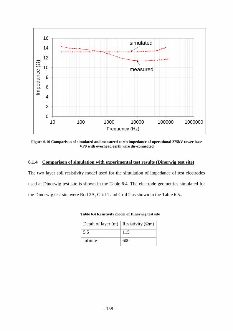
- 158 -
Figure 6.10 Comparison of simulated and measured earth impedance of operational 275kV tower base
VP9 with overhead earth wire dis-connected
6.1.4 Comparison of simulation with experimental test results (Dinorwig test site)
The two layer soil resistivity model used for the simulation of impedance of test electrodes
used at Dinorwig test site is shown in the Table 6.4. The electrode geometries simulated for
the Dinorwig test site were Rod 2A, Grid 1 and Grid 2 as shown in the Table 6.5..
Table 6.4 Resistivity model of Dinorwig test site
Depth of layer (m) Resistivity (Ωm)
5.5 115
Infinite 600
0
2
4
6
8
10
12
14
16
10 100 1000 10000 100000 1000000
Frequency (Hz)
measured
simulatedIm
ped
ance
(Ω)

- 159 -
Table 6.5 List of earth electrodes tested at Dinorwig test site
Type of earth
electrode
Designation used in
the experiments
Material Dimensional details
Single rod Rod 2A Copper 14mm dia., immersed 200cm deep in
water
Grid 1 5m x 5m grid Aluminium 5m x 5m earth grid, 506mm2 at cross
section, immersed 20cm deep in water
Grid 2 5m x 5m grid Aluminium 5m x 5m earth grid, 506mm2 at cross
section, immersed 40cm deep in water
Unlike the Llanrumney test site, there is a close agreement between the simulated and
measured earth impedances at Dinorwig test site for Rod 2A and two depths of 5m x 5m grid
over the frequency range 20Hz to 1MHz as shown in Figure 6.11, Figure 6.12, Figure 6.13
and Figure 6.14. This is due to the relative ease of the representation of the resistivity of the
conducting medium in the form of horizontally layered model for Dinorwig test site. It was
also noted that there are contradictory trends between measurements and simulations above a
frequency of few MHz for both the electrodes. This may be due to the significant
electromagnetic coupling between current injection and potential measurement leads at high
frequencies above few MHz.
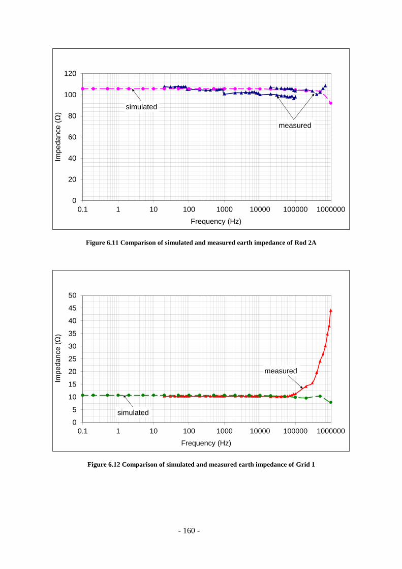
- 160 -
Figure 6.11 Comparison of simulated and measured earth impedance of Rod 2A
Figure 6.12 Comparison of simulated and measured earth impedance of Grid 1
0
20
40
60
80
100
120
0.1 1 10 100 1000 10000 100000 1000000
Imp
eda
nce
(Ω
)
Frequency (Hz)
simulated
measured
0
5
10
15
20
25
30
35
40
45
50
0.1 1 10 100 1000 10000 100000 1000000
Impedance (
Ω)
Frequency (Hz)
simulated
measured

- 161 -
Figure 6.13 Comparison of simulated and measured earth impedance of Grid 2
Figure 6.14 Comparison of simulated and measured earth impedance of single rod at Dinorwig
0
5
10
15
20
25
30
35
40
45
50
0.1 1 10 100 1000 10000 100000 1000000
Impedance (
Ω)
Frequency (Hz)
simulated
measured
0
20
40
60
80
100
120
140
1.E+01 1.E+02 1.E+03 1.E+04 1.E+05 1.E+06 1.E+07 1.E+08
Frequency (Hz)
Imp
ed
an
ce
ma
gn
itu
de
(Ω)
.
Circuit
model
simulation
CDEGS
simulation
Measurement

- 162 -
6.2. Conclusion
The extensive experimental data has been compared with numerical modelling of the test
electrodes. It was observed that the numerical modelling of the test electrodes does not
exhibit the reducing trend of earth electrode impedance with increase in frequency over the
range 20Hz to 120kHz. However the numerical modelling does show sharp reduction in the
earth impedance of earth electrodes above a frequency of few mega-hertz which is mainly
attributed to the capacitive effects in the soil getting dominant above few mega-hertz. It was
also observed that the measured earth impedance of earth electrodes at Llanrumney test site is
different in magnitude to that predicted by the numerical modelling. This was attributed to
the difficulty in representing the heterogeneous soil model in two layer model. However the
measured earth impedance of earth electrodes at Dinorwig test site show a good agreement
which is due to the fact that the homogenous water resistivity is easier to represent in two
layer model.

- 163 -
Chapter 7: Analysis of current and frequency effects on earth
resistance and earth impedance
7.1. Introduction
The results from AC, DC and impulse tests reported in Chapter 5 revealed important
frequency and current magnitude effects on earth resistance and impedance of the various
earth electrodes considered. The calculated and simulated values of earth resistance and
impedance (Chapter 6), however, did not replicate the observed experimental trends showing
a reduction in resistance / impedance over a low frequency and low current range. In order to
explore these findings a more detailed literature search was carried out and an attempt is
made to explain the phenomena involved.
7.2. Soil conduction review
The literature review on soil conduction revealed that there is an increase in the conductivity
of the soil samples tested in the laboratory when the frequency is increased from 1 to 108 Hz
[49]. This effect has been observed by several experimentalists, and this phenomenon is
termed as conductivity dispersion [49] [52] [54] [55]. Figure 7.1 shows a model of electrical
conduction in the soil. As can be seen from Figure 7.1 there are three possible paths of
conduction in the micro-pores of the soil as follows,
a) Solid liquid pathway: Some of the electrical current flows over the soil solid particles
surfaces combined with the electrolytic current flow in the moisture content of the soil
micro-pores.
b) Solid pathway: A small amount of the electrical current flows through the complete
solid pathway.
c) Liquid pathway: A majority of the electric current flows through the liquid pathway.

- 164 -
Figure 7.1 Model of conduction of electric current through soil micro-pores reproduced from [44]
7.3. Analysis of measured effect of frequency on impedance of earth electrode
With reference to the experimental results, Figure 7.2, groups all plots of earth impedances
over frequency of injected current for the various electrodes tested in the field. As can be
seen from the figure, all the electrodes tested show a reduction in measured earth impedance
with increase in frequency over the range 20Hz to 100kHz. To visualise more clearly the
effect of reduction of the measured earth impedance over frequency, the normalised values of
the measured earth impedances were plotted in Figure 7.3. As can be observed from the
figure, there is a decrease of between 10% and 30% in the measured earth impedances of
various electrodes tested in the field.

- 165 -
Figure 7.2 Effect of frequency on earth impedance for various electrodes
Figure 7.3 Normalized effect of frequency on earth impedance
0
20
40
60
80
100
120
140
10 100 1000 10000 100000 1000000 10000000
Imp
ed
an
ce
(Ω
)
Frequency (Hz)
single rod, Dinorwig, 07/08/08
single rod, Dinorwig, 06/08/08
single rod, Llanrumney, 22/08/08
TTB, Llanrumney, 14/07/08
3m x 3m grid, Llanrumney, 02/04/08
cluster of rods, Llanrumney,22/07/08
Isolated VP9, Llanrumney, 21/07/08
Aluminium tape, Llanrumney, 07/08/08
0.5
0.6
0.7
0.8
0.9
1
10 100 1000 10000 100000
No
rma
lize
d im
pe
da
nce
Frequency (Hz)
single rod, Dinorwig
single rod, Llanrumney
Test Tower Base, Llanrumney
3m x 3m grid, Llanrumney
3 rods + horizontal electrode, Llanrumney
Isolated VP9, Llanrumney
5m horizontal electrode, Dinorwig
cluster of rods (8,1,2) with insulated cables connected,Llan

- 166 -
7.4. Frequency dependence of clay water electrolyte properties: an overview
Arulanandan [46] conducted experiments on saturated kaolinite clay-water-electrolyte
systems and found that there are two distinct dispersions, one in the low frequency range (0
to 100 kHz) and the other in the high frequency range (1 MHz to 100 MHz). An increase in
electrical conductivity has also been experimentally observed for clays by [47], [48], [49],
mineralised rocks [50], polymers [51], synthetic membranes [52], ion exchange resins [53]
and polystyrene spheres [54]. The conductivity dispersion characteristics were experimentally
observed in the frequency range of either 0 to 100 kHz or 1 MHz to 100 MHz.
Arulanandan [46] suggested two different mechanisms for these low frequency and high
frequency conductivity dispersions; The increase in conductivity with an increase in
frequency in the low frequency range is due to the increase in the surface conductance of the
soil. The application of the alternating current sets the ions in an oscillatory motion. In clays
and other ion exchangers, the positive counter-ions required to balance the negative fixed
charges on the solid particles are in majority, and hence they impart more momentum to the
water than the co-ions. Thus, there is a net water transfer in the direction of counter-ion
movement. When a current is flowing in the system, there is a net water movement to
accompany the flow. If a low frequency current is passing, there is enough time available for
any pressure gradient to build up. Such a pressure gradient will tend to oppose the flow of the
fluid. Thus, in D.C. steady state, there is an electro-osmotic counter pressure which prevents
the volume flow in the clay water electrolyte solution. The hydraulic flow in the clay water
electrolyte solution is caused by the passage of electric current. The electro-osmotic counter
pressure opposes the hydraulic flow of clay water electrolyte solution, thereby, introducing
the electrical resistivity. At high frequency, when the frequency of the alternating current is
large enough, a stage could be reached when sufficient time is not available for the build up

- 167 -
of a pressure gradient. This stage represents the condition when there is more flow of fluid
and corresponding higher electrical conductivity.
Oliver de Lima et al. [45] developed models for conductivity dispersion and compared it with
the experimental observations of K. Arulanandan [46] for a sodium kaolinite sample (Hydrite
R with 38.8 % water content). It was observed that the conductivity dispersion of sodium
kaolinite sample (Hydrite R with 38.8 % water content) is approximately 0.018 Siemens/m at
100 Hz to 0.025 Siemens/m at 1 MHz. The conductivity dispersion of sodium kaolinite
sample (Hydrite R with 59.5 % water content) is approximately 0.0135 Siemens/m at 100 Hz
to 0.021 Siemens/m at 100 kHz, as shown in Figure 7.4. It was also observed that the
mechanism causing the conductivity dispersion is significantly affected by the size of
particles in clay water electrolyte systems.
Figure 7.4 Conductivity dispersion in soil sample [46]

- 168 -
As seen from Figure 7.4, the increase in conductivity over the frequency range of 20Hz to
100kHz is about 33% of the value at 100kHz. The experimental results for the earth
impedance measurement tests over a frequency range of 20Hz to 100kHz as shown in Figure
7.3, indicate a fall in the impedance value of 10% to 33%. The mechanism of conductivity
dispersion in the soil seems to be the cause of the reduction in the measured earth impedance
with increase in frequency.
Systematic experimental measurements of the electrical properties of shaly materials have
shown that both their conductivity (σ) and permittivity (є) are dispersive in the frequency
domain. Although, individually for water and most silicate minerals, these properties are
almost independent of frequency (ω), the composite properties are appreciably frequency
dependent [55]. If, instead of using a DC source for measurement of resistivity, a variable
low frequency AC source is used, it was found that the measured apparent resistivity of the
subsurface decreases as the frequency is increased [56]. This is because the capacitance of the
earth inhibits the passage of direct currents but transmits alternating currents with increasing
efficiency as the frequency increases [56]. When using a standard four electrode resistivity
spread in a DC mode, if the current is abruptly switched off, the voltage between the potential
electrodes does not drop to zero immediately. After a large initial decrease the voltage suffers
a gradual decay and can take a longer time to reach a zero value. A similar phenomenon is
observed as the current is switched on. After an initial sudden voltage increase, the voltage
increases gradually over a certain time interval to a steady state value. The earth, thus, acts as
a capacitor and stores electric charge and it becomes polarised. The capacitance property of
the earth causes both the transient decay of a residual voltage and variation of apparent
resistivity as a function of frequency.

- 169 -
Laboratory experiments indicated that the electrical energy is stored in rocks mainly by an
electrochemical process [50]. The passage of electric current through a rock as a result of an
externally imposed voltage is accomplished mainly by electrolytic flow in pore fluid. Most of
the rock forming minerals have a net negative charge on their outer surfaces in contact with
the pore fluid and attract positive ions onto this surface. The concentration of the positive
ions extends about 100 µm into the pore fluid, and if this distance is of the same order as the
diameter of the pore throats, the movement of the ions in the fluid resulting from the
impressed voltage is inhibited [52]. Negative and positive ions build up on either side of the
blockage and, on removal of the voltage, the ions return to their original locations over a
finite period of time causing gradually decaying voltage. This effect is known as membrane
polarization or electrolytic polarization [45]. It is most pronounced in clay minerals where the
pores are particularly small. The effect decreases with the increasing salinity of the pore fluid.
When the metallic minerals are present in a rock, an alternative electronic path is available
for current flow.
7.5. Effect of current on the measured earth impedance
As indicated in Chapter 5 the DC tests carried out on earth electrodes at Llanrumney and
Dinorwig have revealed that there is a decrease of more than 20 % in the measured earth
resistance when the injected current is varied from 1mA to 1A. Figure 7.5 shows the plots of
measured earth impedance over the current range 50 mA to 3A for the various electrodes
tested. In general, for the AC tests on the earth electrodes, the reduction in the measured
value of earth impedance was less than 4% as shown in Figure 7.6, when the injected current
was increased from 50 mA to 3A. The reduction in measured earth impedance was less than
1% between 500mA and 3A. However, for one particular electrode viz, the test tower base
(VP9) as shown in Figure 7.6, a more noticeable reduction of up to 7 % was measured over

- 170 -
the current range 50mA to 3A. In order to check the repeatability of the measured values of
tower earth impedance, the AC tests on tower base were repeated; the results of this test
confirmed the previous findings. The decrease of earth resistance with the increase in
magnitude of the DC current is found to be higher than that of the reduction of the earth
impedance with the increase in the magnitude of AC current. It is also observed that the
effect of current on the earth impedance is lower at higher frequency (1 kHz and above)
compared with a lower frequency range (20 Hz to 52 Hz).
Figure 7.5 Effect of current on earth impedance
0
20
40
60
80
100
120
140
160
0.0 0.5 1.0 1.5 2.0 2.5 3.0 3.5 4.0
Current (A)
Imp
ed
an
ce
(o
hm
s)
Single rod, Dino,
31/07/08 & 01/08/08
3m x 3m
grid,
Llan,
02/05/08
Single rod, Llan,
22/08/08
TTB, Llan,
14/07/08
Iso VP9, Llan,
03/07/08

- 171 -
Figure 7.6 Normalized effect of current on earth impedance
7.6. Nonlinear current effect
In an attempt to explain the effect of current density on earth impedance, it was shown that
the measured earth impedances exhibited an increasing trend with increase in current density
in the range of 0.002A/m2 to 0.1A/m
2 and a falling trend above 1A/m
2. It is suggested that the
polarization effect, which is dominant at DC and low frequency AC (up to 50Hz), could be a
possible cause of this current effect. Geo-physical literature survey [50] [56] revealed that the
polarization effect occurs a) inside the micro-pores of the soil where the electric current
transmits between the surface of the soil particles and the pore moisture content, and b) the
interface between metallic electrodes and the soil.
0.92
0.93
0.94
0.95
0.96
0.97
0.98
0.99
1
0.0 0.5 1.0 1.5 2.0 2.5 3.0 3.5 4.0
Current (A)
No
rma
lise
d Im
pe
da
nce
Single rod, Dino,
01/08/08
Single
rod, Llan,
22/08/08
TTB,
Llan,
14/07/08
Iso VP9,
Llan,
03/07/08
f = 50 Hz
f = 20 Hz
f = 5 kHz
f = 1 kHz
f = 52 Hz
f = 10 kHz
f = 1 kHz f = 20 Hz f = 5 kHz
f = 1 kHz
f = 10 kHz
f = 52 Hz

- 172 -
The polarization impedance of metal electrodes and electrolyte interface (Zp) operated at low
current density (0.025mA/cm2) can be calculated as given in [59] using the following
equation,
22005.0
BfAf
SZ p ------------- (7.1)
Where S is the surface area of the electrode in cm2 and Zp is kΩ
A review of literature by Geddes [59] showed that β ranged from 0.38 to 0.78 for several
common electrode metals. Table 7.1 shows the values of constants A, B, α and β for the
common electrodes tested by Ragheb et al. [59] at 100Hz to 100kHz, at current density of
0.25A/m2 [59].
Table 7.1 Values of constants for different electrode metals tested
Electrode metal A B α β
Stainless steel 989 1849 0.760 0.734
Copper 44.3 45.2 0.487 0.482
Aluminium 2427 10814 0.899 0.874
Table 7.2 shows the calculated values of polarization impedance for different electrodes
tested at Llanrumney and Dinorwig for the range of current densities below 0.25A/m2
calculated form the Equation (7.1)
As can be seen from Table 7.2, the polarization impedance for the electrodes tested in the
field is negligible when compared with the measured values of earth impedances above 50Hz
and the low frequency (ABEM 1Hz) measurements show noticeable polarization effects.
The non-linear effect of current magnitude has been observed by Katsube et al. [61] on dry
rock samples and conductive minerals and by Ragheb and Geddes [62] on metallic electrodes
in electrolytes. Katsube et al. [61] have shown that the specimen of rock samples

- 173 -
(serpentinite, asbestos) and conductive minerals (pyrite - FeS2, Cubanite – CuFe2S3, galena
PbS) exhibit the nonlinear current effect. They observed that the nonlinear phenomena
occurred in the serpentinite and galena samples above a critical current density of
3.1 x 10⁻¹⁰
A/cm2 at 10
-2Hz and 3.1 x 10
-7A/cm
2 at 10Hz as shown in Figure 7.8. At the test
frequency of 52Hz (used in the field), the extrapolated nonlinear density would be above 3.1
x 10-6
A/cm2 (above 0.03A/m
2). This is in close agreement with the field tests results which
indicate nonlinearity above a current density of 0.04A/m2, as shown in Figure 7.9. The
frequency response and current dependence of the electrode-electrolyte interface resistance
observed by Ragheb and Geddes [62], shown in Figure 7.8 qualitatively agrees with the test
results of earth impedance measurements for electrodes tested at Llanrumney at different
current magnitudes over the frequency range 20 Hz to 100kHz. The conduction of current in
the soil is mainly electrolytic in nature. The combination of soil water content in the pores
and the soil particles (clay particles) forms an interface through which conduction of
electrical current occurs. Katsube et al. [61] suggested that the electrical non-linear
phenomena occur at the micro-fractures of the soil of less than 1.0 micron thickness or at the
moisture levels that have accumulated thickness of 80 microns. Their calculation was based
on the assumption that the dielectric constant of water is 80.

- 174 -
Figure 7.7 Current dependence of electrode electrolyte interface observed by Ragheb and Geddes
Polarization effect observed in the literature (reproduced from Katsube et. al., “Electrical nonlinear
phenomenon in rocks”, Geo-physics Vol. 38, No.1, February 1973, P. 106-124
Table 7.2 Calculated values of polarization impedance
Electrode type
Surface
area
(m2)
Electrode
material
Frequency
(Hz)
Polarization
impedance
(Ω)
Measured
earth
impedance
(Ω)
3 m x 3m grid,
Llanrumney 2.0160 Aluminium
1 2.75 18.64
52 0.087 12.22
100000 0.00012 9.39
Test tower base,
Llanrumney 7.7760 Steel
1 0.135 23.39
52 0.0073 21.22
50000 7.2E-03 19.26
Isolated VP9,
Llanrumney
7.7760 Steel
1 0.135 14.80
52 0.0073 13.61
10000 1.5E-04 11.84
Rod 2, Dinorwig 0.0335 Copper
1 0.945 123.33
52 0.14 122.89
100000 0.0036 109.38
Rod 1,
Llanrumney 0.0605 Copper
1 0.523 63.87
52 0.078 57.65
100000 0.002 51.26
Grid 5m x 5m,
Dinorwig 6.7200 Aluminium
52 0.026 10.27
100000 3.5E-05 11.26

- 175 -
Figure 7.8 Frequency response and current dependence of the electrode-electrolyte interface resistance
observed by Ragheb and Geddes [62]
Figure 7.9 Polarization effect observed during field tests (Effect is pronounced at lower frequencies
~20Hz to 100Hz)

- 176 -
7.7. Comparison of variation of normalized impedance with current density
Previously reported field and laboratory a.c. tests have shown a trend of reduction of
resistance/impedance of the test electrode of between 2% and 9% over the current range of
between 10mA to about 5A. However, different rates of reduction in earth resistance with
current were observed for different electrodes. Further calculations were carried out so that
the values of earth resistance could be expressed as a function of current density at the
electrode surface. The calculation of current density was achieved by dividing the total
injected current by the total earth electrode surface area in the earth medium. It should be
noted that the current density, as calculated, is an approximate average value. The current
density at a particular point on the electrode varies according to the local surface area and
position relative to the centre and extremity of the electrode. Figure 7.10 (a) to (d) show the
earth resistance of rod, rods cluster, grid, TTB, isolated VP9 and resistance of laboratory test
cell as a function of current density over the range 0.01 to 30A/m2. From the results shown in
the figures it can be said that the electrode resistance is relatively constant up to a current
density of 1A/m2. Between a current density of 1 and 30A/m
2, the earth resistance falls. This
trend applies for all rods, rods clusters, grids horizontal electrodes at both Llanrumney and
Dinorwig. However, there is one exception relating to the test tower base at Llanrumney. For
this particular electrode, the reduction in earth resistance is much greater and it occurs over a
range of much lower current density.

- 177 -
Figure 7.10 Comparison of normalized effect of current density on earth impedance
7.8. Conclusion
The geological literature survey revealed that there is conductivity dispersion in the clay
water electrolyte solution when it is subjected to higher frequency electrical current. The
conductivity dispersion is a phenomenon by virtue of which the conductivity of the clay
water electrolyte increases to about 33% over the frequency range 20Hz to 100kHz. This
phenomenon seems to be responsible for the reduction of earth electrode impedance with the
increase in frequency. The geological literature survey also showed that the polarisation
effect in the soil electrolyte tends to be pronounced at low frequency. The non-linear effect of
current magnitude as a result of the polarisation effect in the soil seems to be responsible for
the pronounced effect of DC current magnitude on the impedance of earth electrodes. It was

- 178 -
observed in the geological literature survey that the nonlinear phenomena occurred in the
serpentinite and galena samples above a critical current density of 3.1 x 10⁻¹⁰
A/cm2 at 10
-2Hz
and 3.1 x 10⁻⁷
A/cm2 at 10Hz. At the test frequency of 52Hz (used in the field), the
extrapolated nonlinear density would be above 3.1 x 10⁻⁶
A/cm2 (above 0.03A/m
2). This is in
close agreement with the field tests results which indicate nonlinearity above a current
density of 0.04A/m2. The frequency response and current dependence of the electrode-
electrolyte interface resistance observed by Ragheb and Geddes [62] qualitatively agrees with
the test results of earth impedance measurements for electrodes tested at Llanrumney at
different current magnitudes over the frequency range 20 Hz to 100kHz.

- 179 -
Chapter 8: Conclusion and Future Scope of Work
The survey of various earthing measurement techniques revealed that the Smart Ground
Meter which operates at a maximum frequency of 400Hz would underestimate the earth of
transmission tower connected with the overhead shield earthing wire. As seen from the
experiments performed on the tower earth measurements of VP9 transmission tower shown in
Chapter 5.6.2 (Figure 5.28) the frequency required to measure the local earth resistance of the
tower base connected with the shield wires is about 30kHz. This aspect shows that the
variable frequency and impulse measurements are important tool during the field tests. It was
also seen during the field tests that measuring the earth resistance of various test electrodes at
low DC currents (DC currents ranging from 1mA to 10mA) overestimates the value of the
earth resistance. Moreover, it was observed that, the current density in the earthing electrodes
during the tests plays an important role in connection with the measured value of the earthing
resistance. A care has to be taken to inject the current such that a sufficient current density is
achieved during the tests to achieve the appropriate value of the measured earth resistance of
the test object.
8.1. Advantages and limitations of different earthing measurement techniques
A number of approaches have been used during the course of this project to
measure/calculate the earth resistance / earth impedance of a variety of earth electrode
systems. These are as follows
1) Switched DC for earth resistance measurement
2) Variable frequency AC for earth impedance measurement
3) Impulse
a. Calculation of impulse resistance from instantaneous voltage at peak current over the
value of peak current V@Ipeak/Ipeak

- 180 -
b. FFT analysis to obtain frequency response
The main findings in this area including the advantages and limitations of these techniques
are summarized as follows:
i) Switched DC Technique:
In this technique, the injected current is typically supplied from a battery driven inverter as a
symmetric square wave DC source (typically 90 to 130Hz for commercial ‘earth testers’ and
around 1Hz for ‘geo-physical’ meters). Such instruments have an output voltage limited to
50V and delivering currents ranging from 1mA to 1A. However, the magnitude of earth
resistance measured with this type of instrument may not be representative of the value of the
earth impedance under a.c. power frequency (depending on the size of earthing system) nor
the characteristics of the electrode under impulse conditions. Experimental tests in this
project have demonstrated that both the magnitude of injected current and switching
frequency affect the measured value of the resistance. The current magnitude effect is greater
at lower switching frequencies and the measurement results have shown that, over this
relatively low-current range, the effect of current is quite small above 100mA. Therefore, the
use of a higher DC switching frequency (e.g. between 90 to 130Hz), above the power
frequency, is beneficial in reducing polarisation effects and mitigating the effects of power
frequency noise. However, over this range of frequency, the inductive component of large
area earthing systems may be significant and this will affect the measurement such that the
reading may neither represent the earth resistance nor the earth impedance of the system.
ii) Variable frequency AC Technique:
The Cardiff University impedance measurement system, IMS, injects variable frequency
current and, with suitable measurement of earth potential rise at the point of current injection,
the frequency response of the earthing system is obtained. Moreover, the frequency selective
lock-in amplifiers provide rejection of noise. Experience has shown that the impedance at

- 181 -
50Hz can be determined by linear interpolation when using test injection frequencies as close
as 2Hz either side of 50Hz, i.e. 48Hz and 52Hz. AC tests at higher frequencies can be used to
measure the earth resistance of an individual transmission tower while connected to its
overhead earth wire (when the injection frequency is set higher than 50kHz). It should be
noted that the time taken for acquiring the required current and EPR data using the current
setup is significant, although this limitation can be overcome if the process of data acquisition
is automated. Under AC tests, care is required to ensure that there is sufficient distance
between the main and auxiliary earth electrodes to avoid coupling between the current
injection and potential measurement leads, and the potential reference electrode is located
sufficiently far away to obtain a reliable earth reference point.
iii) FFT from impulse and calculating the impulse resistance from the
waveforms:
In this technique, the plot of impedance over a desired frequency range is obtained from the
FFT of the impulse signals (injected current and EPR). The results obtained with this
technique have shown good agreement with those obtained from variable AC tests. The
frequency components obtained from the FFT of the impulse signals are limited by the
sampling rate and the sampling depth (time period over which the signal is acquired).
Therefore, in this investigation, two separate impulse waveforms were used; one with a fast
rise time ~ 1µs, and the other with long tail (~ 50ms). In this way, frequency components
ranging from 20Hz to more than 100kHz could be obtained from the FFTs of the impulse
signals. This approach may be susceptible to error if the signal to noise ratio is not
sufficiently high.
Another method related with impulse injection is to calculate the value of impulse resistance
as V@Ipeak / Ipeak. At the instant when the injected current waveform reaches its peak value
in an inductive circuit, the rate of rise of current becomes zero, and the ratio of EPR to

- 182 -
current is a representative of impulse resistance. The effect of current magnitude (although
lower compared to low frequency currents) was observed for the impulse waveforms.
Moreover, the magnitude of the impulse resistance was also affected by the rise time of the
impulse (i.e. lower value of resistance in the case of faster rise time)
In summary the investigations carried out in this work have allowed to reach practical
conclusions on the suitability and limitations of existing / available earth testing measurement
techniques and instrumentation. These conclusions are as follows,
Switched DC test techniques to measure electrode earth resistance should be limited to small
area earthing systems.
For low-current test instruments, a certain minimum current may be required e.g. 100mA.
Variable frequency AC tests require very good noise rejection capability in order to allow
injection close to the power frequency and hence accurate determination of power frequency
earthing impedance.
Impulse tests may be used to determine the impulse resistance with relatively low
source power requirements, although the use of FFT to determine the power frequency
impedance will require further investigation under conditions of realistic background noise.
8.2. Validity range of earthing measurement techniques
From an analysis of measurement results from the project test programme, consideration has
been given to determine a feasible range of test current magnitude and a frequency range
under DC / AC test conditions. In this work it was clearly shown that the non-linear effect of
current is greater at lower frequencies.
The switched DC test instrument such as ABEM Terrameter (approx. 1Hz) has shown the
highest reduction in measured resistance (up to 20%) over the range 1mA to 1A. Further
reduction in measured resistance may occur above 1A. Switched DC tests carried out over a

- 183 -
higher frequency range (105Hz and 160Hz) using the DET2/2 did not reveal any significant
change in measured resistance for any of the test electrodes at the two different current
magnitude settings (7mA and 50mA).
For a.c. tests, in the 48-52Hz frequency range, the phenomenon of resistance reduction with
current is less pronounced (7% over the current range 10mA to 3.5A). The variable frequency
a.c. tests indicated that the current magnitude effect reduces appreciably over the frequency
range 20Hz to 1kHz, above which frequency the reduction of resistance with current
magnitude is negligible. Generally, there was close agreement between the a.c. test using the
Cardiff University IMS system at about 50Hz and the DET2/2 results for the tested electrodes
at Llanrumney and Dinorwig (excluding the VP9 operational tower earthing system). It is
possible that by adopting relatively higher switched DC frequencies (up to 1kHz) for small
earth electrodes, an overestimation of earth resistance due to the non-linear effect of current
can be minimised. However, this would only be applicable to small-area earthing systems
with low inductive reactance at the test frequency.
Impulse tests allowed investigation of earth resistance at higher currents up to 8A. It was
found that by using currents with impulse rise-times in the range 2-60μs, the measured
resistance values (impulse resistance) for the tested electrodes were up to 10% lower than
those obtained at the power frequency a.c. tests. However, FFT analysis of impulse
recordings gave values very close to those obtained using the variable frequency a.c. tests,
including promising close agreement with the ‘50Hz’ resistance values.
8.3. Feasible current and frequency ranges for earth impedance measurement
With the ABEM Terrameter, DC currents within the range of 1mA to 1A have been used in
the past to measure the earth resistance. Extensive testing revealed that there is a pronounced
non-linear behaviour within the DC current range 1mA to 100mA (reduction of measured

- 184 -
earth impedance with increase in current magnitude). The performance of earth impedance
within this current range has not yet been fully explored and clarified. However, it was
established experimentally that the earth impedance readings for current magnitudes above
100mA DC were within the acceptable range (within 5% of the measured values by DET
2/2).
For the case of AC currents used in the field (few tens of mA to few amperes), the earth
impedance measurements (20Hz) was seen to exhibit a maximum reduction of 4% for
different electrodes tested (except for the test tower base where it was up to 7%). It was also
noted that the effect of current magnitude falls appreciably as the test frequency is increased
above 1kHz. Hence, it would be useful to use current magnitudes of 50mA to 100mA at
frequencies above 1kHz to measure earth impedance. Moreover, the use of higher frequency
levels would reduce the effect of power frequency background noise.
The use of test frequencies of 20Hz to 100kHz in the field tests have shown that there is up to
30% reduction in the measured earth impedance over this frequency range. It would be useful
to use the swept frequencies of this range in the practical earthing impedance measurement
instrument to evaluate earth impedance values at the frequencies of interest.
The set-up of the injection system near the test object is helpful to reduce electromagnetic
coupling, and the test results obtained with this set up have provided comparable results for
different earth electrodes tested. As seen from the experiments conducted so far, the input
voltage requirement for impedance measurement increases as the frequency of injected
current is increased. This is because when the injection system is placed near the test object,
the return current lead (typically 50 to 100m long) will contribute to the inductance which
increases linearly with injected current frequency. This means that the input voltage required
to inject the desired magnitude of current at higher frequency is larger compared with the

- 185 -
input voltage required to drive the same amount of current in the earthing system at lower
frequency. If a low inductance lead is used for the return current circuit, then the input
voltage requirement of the injection system may be reduced.
The impulse current injection tests have been conducted on various earthing electrode
systems. An approach to obtain the FFT spectrum from the time domain impulse signals of
current and EPR (earth potential rise) has been introduced in this work. This investigation
demonstrated that the highest frequency under which the response of an earthing system can
be computed by FFT analysis is the frequency component of the initial rise of the impulse
current signal. The rise time of the injected current signal is also influenced by the total
inductance of the earthing measurement circuit. If the inductance of the measurement circuit
is reduced, by selecting low inductance return lead, then the highest frequency under which
the response of an earthing system is computed can be increased. The lowest frequency
component under which the response of an earthing system impedance can be computed is
given by the inverse of the product of the sampling time interval and the sampling depth. For
e.g. if the (10 % to 90%) linear rise time of the current signal is 1μs, the sampling interval is
200ns and the sampling depth is 500ksamples, then the lowest and highest frequency range
under which the response of the earthing system can be computed is 100 Hz to 1 MHz in
steps of 100 Hz each. This analysis will yield a frequency domain response which is
comparable to that obtained from variable frequency test results. It is planned to adopt these
findings in the future impulse current injection tests.
8.4. Future scope of work
In the present project, the effect of current magnitude has been analysed to a fair extent. It
was observed that the current density into the earth electrode during the tests has important
correlation to the effect of current on the measured earth impedance. In future, it would be

- 186 -
useful to further investigate the effect of current density, taking into consideration the
materials such as copper, aluminium and steel. It could be useful to find a critical current
density point in the earth electrode beyond which the current magnitude effects on the
measurements could be reduced.
It would be useful to explore the possibility of developing the computer models that can
accommodate the soil polarisation effects leading to the nonlinear current effect phenomenon
and the conductivity dispersion effects exhibiting the frequency dependence of the earth
impedance measurements.
It is well known that the impulse measurement tests have performed by several
experimentalists in the hundreds of amperes range already and such results could be analysed
using the proposed FFT analysis introduced in this work.
Similarly, the effect of frequency on the measured earth impedance was investigated up to a
frequency of 100 kHz. Above 100 kHz the electromagnetic coupling effect is expected to be
significant which may distort the measurement. A possible solution is to use low inductance
co-axial cables for measurement purposes whenever possible. If the effect of frequency is to
be studied beyond 100 kHz range, and up to 1 MHz range, it would be useful to characterise
the behaviour of earthing systems for the lightning characteristic frequency.

- 187 -
References
[1] Leonid D. Grcev, "Transient Electromagnetic Fields Near Large Earthing Systems",
IEEE Transactions on Magnetics, Vol 32. No. 3 , pp. 1525-1528, May 1996
[2] C. F. Dalziel, "Electric shock hazard", IEEE Spectrum, pp. 41-50, February 1972.
[3] C. F. Dalziel and W.R.Lee, "Re-evaluation of lethal electric currents", IEEE
Transactions on Industry Applications, vol. IA-20, No. 4, pp. 1089, July 1984.
[4] P. G. Beigelmeier and W.R.Lee, "New considerations on the Threshold of Ventricular
Fibrillation for AC shocks at 50-60 Hz", IEE Proceedings, Physical Science,
Measurement and Instrumentation, Management and Education - Reviews, Vol. 127,
No. 2, pp. 103-110, March 1980.
[5] "IEEE guide for safety in AC substation earthing", IEEE Std. 80-2000, pp. i-192,
2000.
[6] L. D. Grcev and M. Heimbach, "Frequency dependent and transient characteristics of
substation earthing systems", IEEE Transactions on Power Delivery, Vol. 12, No. 1,
pp. 172-178, January 1997.
[7] M. Heimbach and L. D. Grcev, "Grounding system analysis in transients programs
applying electromagnetic field approach", IEEE Transactions on Power Delivery,
Vol. 12, No.1, pp. 186-193, January 1997.
[8] Z. Rong, H. Jinliang, and G. Zhicheng, "Novel Measurement system for Grounding
Impedance of Substation," IEEE Transactions on Power Delivery, Vol. 21, No.2, pp.
719 - 725, April 2006.
[9] A. P. S. Meliopoulos, G. Cokkinides, H. Abdallah, S. Duong, and S. Patel, "A PC
based ground impedance measurement instrument", IEEE Transactions on Power
Delivery, Vol. 8, No.3, pp. 1095-1106, July 1993.

- 188 -
[10] P. J. Higgs, "An Investigation of Earthing Resistances", Journal of the Institution of
the Electrical Engineers, Vol. 68, No.402, pp. 736-705, June 1930.
[11] “IEEE Guide for measuring earth resistivity, earth impedance and earth surface
potentials of a ground system, Part I - Normal Measurements”, IEEE Std. 81-1983.
[12] Hideki Motoyama, “Experimental and analytical studies on lightning surge
characteristics of ground mesh", Electrical Engineering in Japan, Vol. 160, No.4, pp.
16-23, September 2007.
[13] Sunde ED, "Earth conduction effects in transmission systems", Dover Publications
Inc.; New York edition, 1968, ISBN-10: 0486618919, ISBN-13: 978-0486618913.
[14] Portela C, “Soil electromagnetic behaviour”, International conference on Grounding
and Earthing, Proceedings, pp 53-58, Belo, Horizonte, Brazil, April 1998.
[15] Leonid Grcev, “Improved design of power transmission line earthing arrangements
for better protection of against effects of lightning, Proceedings of the International
Symposium on Electromagnetic Compatibility (EMC’98 ROMA), Paper C1-7, pp.
100-103, Rome, Italy, 1998.
[16] H Griffiths and N Pilling, Chapter 8, “Earthing”, “Advances in High Voltage
Engineering”, IEE Power and Energy Series 40, Edited by A. Haddad and D. Warne,
The Institution of Electrical Engineers, UK, 2004, ISBN# 0 85296 158 8
[17] Dawalibi F and Mukhedkar D, “Resistance measurement of large grounding systems”,
IEEE Power Engineering Society Meeting, IEEE paper F79656-0, Vancouver, 1979.
[18] Tagg G F, “Earth Resistances”, George Newnes Ltd., London, 1964, ISBN 003210
[19] Tagg G F, “Measurements of the resistance of an earth electrode system covering a
large area", Proceedings of the Institution of Electrical Engineers, Vol. 116, No.3, pp.
475-479, March 1969.

- 189 -
[20] Curdts E B, “Some of the fundamental aspects of ground resistance measurements",
AIEE Transactions, Vol. 77, No.1, pp 760, 1958.
[21] Dawalibi F and Mukhedkar D, “Ground electrode resistance measurement in non-
uniform soils”, IEEE Transactions on Power Apparatus and Systems, Vol. PAS-93,
No. 11, pp. 109 – 116, January 1974.
[22] Dawalibi F and Mukhedkar D, “Modelling of potential distribution around a
grounding electrode”, IEEE Transactions on Power Apparatus and Systems, Vol.
PAS-92, No. 5, pp. 1455-1459, 1973.
[23] Tagg G F, “Measurements of earth electrode with particular reference to earth
electrode systems covering a large area", Proceedings of the Institution of Electrical
Engineers, Vol. 111, No.12, pp. 2118 - 2130, Dec 1964.
[24] “Getting Down to Earth, A Practical Guide to Earth Resistance Testing”, by Megger,
1-866-254-0962, www.megger.com
[25] Liwei Li, Jiyan Zou, Hui Sun, “Research on the New Clamp-on Grond Resistance
On-line Tester Based on AC Variable Frequency”, Proceedings of the 6th World
Congress on Intelligent Control and Automation, Vol. 2, pp. 5286-5289, Dalian,
China, June 21 - 23, 2006.
[26] Kruger M, “Measurement of overhead line and cable impedance values, earth
impedance of large substations and electromagnetic interference between overhead
lines and signal cables using a new technology”, International Conference on
Developments in Power System Protection, Vol.1, pp. 240-243, April 2004.
[27] A.P.Meliopoulos, George Cokkinides, Hanna Abdallah, Steven Duong, Shashi Patel,
“A PC Based Ground Impedance Measurement Instrument” , IEEE Transactions on
Power Delivery, Vol.8, No.3, pp.1095-1106, July1993

- 190 -
[28] A.P.Meliopoulos, Shashi Patel, G. J. Cokkinides, “A New Method and Instrument for
Touch and Step Voltage Measurements", IEEE Transactions on Power Delivery,
Vol.9, No.4, pp. 1850-1860, October 1994.
[29] Jinxi Ma and Farid P. Dawalibi, “Grounding Analysis of a Large Electric Power
Station”, International Conference on Power System Technology, pp.1-6, 2006.
[30] A.J. Surtees, F.D. Martzloff and A. Rousseau, “Grounding for Surge Protective
Devices Ground Resistance versus Ground Impedance”, IEEE Power Engineering
Society General Meeting, 2006.
[31] "ENA Power System Earthing Measurement Guide", EG0, Part - I, Management
Principles, Draft Issue, August 2009.
[32] H. Griffiths, P. Jones, D. Tomlin, N. Harid, A. Haddad, “Proposal for Measurement of
Earth Impedance at High Voltage Electricity Installations Using Variable Frequency
Injection", International Conference on Grounding and Earthing and 2nd International
Conference on Lightning Physics and Effects, Brazil, November 2006.
[33] Jong-kee Choi, Yong-ho Ahn, Sun-guen Goo, Kijun Park, Jin-yul Yoon and Gil-jo
Jung, “Direct Measurement of Frequency Domain Impedance Characteristics of
Grounding Systems”, International Conference on Power System Technology, Vol. 4,
pp. 2218-2221, 2002.
[34] L. Bellaschi, “Impulse and 60 cycle characteristics of driven grounds”, Transactions
of the American Institute of Electrical Engineers, Vol. 60, No. 3, pp. 123-128, 1941
[35] L. Bellaschi, “Impulse and 60 cycle characteristics of driven earths”, in II Trans.
AIEE, vol. 61, 1941
[36] R. Verma, D. Mukhedkar, “Impulse impedance of buried ground wire”, IEEE
Transactions on Power Apparatus and Systems, Vol. PAS-99, No. 5, pp. 2003-2007,
1980.

- 191 -
[37] B.R. Gupta, B. Thapar, “Impulse impedance of grounding grids”, IEEE Transactions
on Power Apparatus and Systems, Vol. PAS-99, No. 6, pp. 2357-2362, 1980.
[38] M. Loboda, R. Kostzaluk, “Model Tests of Surge Properties of Grounding Systems in
Lightning Protection”, 16th International Conference on Lightning Protection, R-5.03,
Szeged, Hungary, 1981.
[39] A. L Vainer, “Impulse characteristics of complex earth grids”, Electrical Technology,
USSR, Vol. 1, 1966
[40] R. Kostzaluk, M. Loboda, D. Mukhedkar, “Experimental Study of Transient Ground
Impedances”, IEEE Transactions on Power Apparatus and Systems, Vol. PAS-100,
No. 11, pp.4653-4660, 1981.
[41] Carlo Mazzetti, Giuseppe M. Veca, “Impulse behaviour of ground electrodes”, IEEE
Transactions on Power Apparatus and Systems, Vol. PAS-102, No. 9, pp. 3148-3156,
1983.
[42] Ulrich Hauser-Ehninger,"A measurement system for the monitoring and measurement
of earthing grid performance at large high voltage substations", PhD Thesis, Cardiff
University, September 2007.
[43] D. Guo, D. Lathi, N. Harid, H. Griffiths, A. Haddad, A. Ainsley, "Large-scale
Earthing Test Facilities at Dinorwig Power Station", International Conference on
Condition Monitoring and Diagnosis, pp.808-811, Beijing, China, April 21-24, 2008.
[44] D. L. Corwin, Leesch, S.M., "Apparent Soil Electrical Conductivity Measurements in
Agriculture," Computers and Electronics in Agriculture, Vol. 46, No. 1-3, pp. 11-43,
2005.
[45] A. L. Olivar de Lima and M. M. Sharma, "A Generalised Maxwell Wagner Theory
for Membrane Polarization in Shaly Sands," Geophysics, Vol. 57, No.3, pp. 431-440,
1992.

- 192 -
[46] K. Arulanandan, "Hydraulic and Electrical Flows in Clays," Clays and Clay Minerals,
vol. 17, No.2, pp. 63-76, 1969.
[47] V. Vacquier, C. R. Holmes, P. R. Kitzinger, and M. Lavergne, "Prospecting for
ground-water by Induced Effect Polarisation," Geophysics, Vol. 22, No.3, pp. 660-
687, 1957.
[48] H. W. Oslen, "Hydraulic Flow Through Saturated Clays," Clays and Clay Minerals,
Vol. 9, No. 1, pp. 131-161, 1960
[49] J. K. Mitchell and K. Arulanandan, "Electrical Dispersion in Relation to Soil
Structure," Journal of Soil Mechanics and Foundations Division, Vol. 99, No. 12, pp.
1113 -1133, 1973.
[50] T. R. Madden and D. J. Marshall, "Induced Polarisation - A Study of its Causes and
Magnitudes in Geological Materials," U.S. Atomic Energy Commission Report,
RME-3160, 80, 1959.
[51] W. Juda and W. A. McRae, "Ion Exchange Material and Method of Making and
Using the Same", US patent 2,636,851, 1953.
[52] K. S. Spiegler and K. Arulanandan, "Radio Frequency Measurements of Ion
Exchange Membranes," Research and Development Report No. 353, U.S.
Government Printing Office, Washington D.C., Report to office of Saline Water, U.S.
Department of the Interior, Washington D.C., 1968.
[53] S. B. Sachs and K. S. Spiegler, "Radio Frequency Measurements of Porous
Conductive Plugs. Ion-Exchange Resin-Solution Systems," Journal of Physical
Chemistry, Vol. 68, No. 5, pp. 1214-1222, 1964.
[54] H. P. Schwan, G. Schwarz, J. Maczuk, H. Pauly, "On the Low Frequency Dielectric
Dispersion of Colloidal Particles in Electrolyte Solutions," Journal of Physical
Chemistry, Vol. 66, No.12, pp.2626-2635, 1962.

- 193 -
[55] G. R. Olhoeft, "Low Frequency Electrical Properties," Geophysics, Vol. 50, No.12,
pp. 2492-2503, 1985.
[56] M. Brooks, P. Kaerey, Ian Hill "An Introduction to Geophysical Exploration", 3rd
Edition, Wiley-Blackwell Publishing, 2002, ISBN: 978-0-632-04929-5.
[57] H. P. Schwan, "Alternating Current Electrode Polarisation," Biophysik, Vol. 3, No.2,
pp. 181-201, 1966.
[58] H. P. Schwan, "Linear and Non Linear Electrode Polarisation and Bilogical
Materials," Annals of Biomedical Engineering, Vol. 20, No.3, pp. 269-288, 1992.
[59] T. Ragheb and L. A. Geddes, "The Polarisation Impedance of Common Electrode
Metals Operated at Low Current Density," Annals of Biomedical Engineering, vol.
19, No.2, pp. 151-163, 1991.
[60] H. H. Sun and B. Onaral, "A Unified Approach to Represent Metal Electrode
Polarization," IEEE Transactions on Biomedical Engineering, Vol. BME-30, No.7,
pp. 399-406, 1983.
[61] T, Katsube, R. Ahrens, L. Collett, “Electrical Nonlinear Phenomenon in Rocks”,
Geophysics, Vol. 38, No. 1, pp. 106-124, 1973.
[62] Ragheb and Geddes, “Electrical Properties of Metallic Electrodes”, Medical and
Biological Engineering and Computing, Vol.28, No.2, pp.182-186, 1990.
[63] R.D. Southey and F.P. Dawalibi, “Improving the reliability of power systems with
more accurate grounding system resistance estimates”, IEEE International Conference
on Power System Technology, Vol. 1, pp. 98-105, Kumning, China, 2002
[64] K. Arulanandan, "Hydraulic and Electrical Flows in Clays," Clays and Clay Minerals,
vol. 17, No.2, pp. 63-76, 1969.

- 194 -
[65] V. Vacquier, C. R. Holmes, P. R. Kitzinger, and M. Lavergne, "Prospecting for
ground-water by Induced Effect Polarisation," Geophysics, Vol. 22, No.3, pp. 660-
687, 1957.
[66] Harid N, Griffiths H, Haddad A, Walker K, "Soil Resistivity Mapping of Non-
Homogeneous Soils", 13th International Symposium on High Voltage Engineering,
pp. 554, Paper P.03.31 Delft, Holland, 2003.
[67] The CDEGS software package (Current Distribution, Electromagnetic Fields,
Grounding and Soil Structure Analysis), Integrated Software for Power System
Grounding/Earthing, Electromagnetic Fields and Electromagnetic Interference Safe
Engineering Services & Technologies Ltd. Canada
[68] Leonid Grcev and Marjan Popov, "On High-Frequency Circuit Equivalents of a
Vertical Ground Rod", IEEE Transactions on Power Delivery, Vol. 20, No. 2, pp.
1598-1603, 2005
[69] CIGRE Working Group C4.2.02: ‘Methods for measuring the earth resistance of
transmission line towers equipped with earth wires’, CIGRE Publication, 2005.
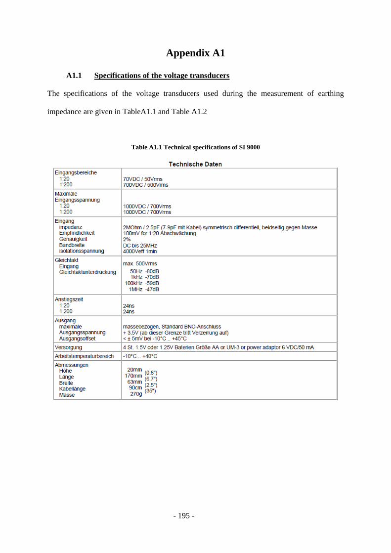
- 195 -
Appendix A1
A1.1 Specifications of the voltage transducers
The specifications of the voltage transducers used during the measurement of earthing
impedance are given in TableA1.1 and Table A1.2
Table A1.1 Technical specifications of SI 9000

- 196 -
Table A1.2 Technical specifications of DP25
A1.2 Specifications of the current transducers
The specifications of the current transducers used during the measurement of earthing
impedance are described in the following sections. The specifications of the current
transducers are shown in the Table A1.3 and Table A1.4
A1.2.1 LILCO BROADBAND CURRENT TRANSFORMER
These current transformers are designed for use as general laboratory instruments
where band width and high-frequency response are to be combined with ease of use.

- 197 -
Model 58MH100
Dimensional Details of LILCO Current Transformer Model 58MH100

- 198 -
Table A1.3 Specifications of LILCO current transformer
Model
number
Output
V/A(1)
RECTANGULAR
PULSE
SINEWAVE
DC
saturation
current
Isat
A
Max.
rms
current
Irms
A
Peak
current
Ipeak
A
Droop
%/ms
Rise
time
ns
I-t
Capability
3dB
Bandwidth Ipeak/f
A/Hz
No
bias
mA s
With
bias
mA s
lf
Hz
hf
MHz
58MH100 0.10 1 20 300 500 1.5 20 2.0 2.0 100 5000
NOTES:
Source impedance - All models have a source impedance of 50R
Load impedance - In the above tables this is assumed to be >50k
50R load - With a 50R load I-t capability is increased by between 20% and 80% and droop
and lf cut-off point are reduced by a factor of 0.6 to 0.85. A 50R load at the receiver and a
50R line should be used where long cables are employed or where the highest frequency
response is required.
Output – Accuracy +/-0.5% at mid-log frequency point, +/-2% within one decade of 3dB
cut-off points. The use of a 50R load will halve the sensitivity
I-t No bias – Lilco broadband current transformers do not require the application any biasing
current to achieve this level of I-t. The use of a 50R load will enhance the I-t capability
significantly.
I-t with bias – these levels are achieved with a dc off-set current equal to Isat. The use of a
50R load will enhance the I-t capability further

- 199 -
58M0020 and 58D0020 – these broadband current transformers have been introduced to
satisfy the measurement demands of EN61000-4-11
A1.2.2 Stangenes Pulse Current Transformer
These current transformers were mainly used for accurately measuring fast impulse currents.
The placement of conductor carrying fast impulse currents in the centre of the axis of the core
was maintained during measurements.
Stangenes Pulse Current Transformer
Table A1.4 Specifications of Stangenes current transformer
Model
No.
Output
(volt/amp)
Accuracy
±0.5%
Inner
Diameter
(inches)
Max.
Current
(amperes)
Peak
Max.
Current
(amperes)
Rms
Square
Pulse
Rise Time
(nanosec)
Square
Pulse
Droop
(%/µsec)
Square
Pulse
IT max.
(amp.sec)
3-0.1A 0.1 2.87 5 k 30 20 0.015 0.03