improving viability of electric taxis by taxi service strategy optimization: a big … · index...

1

Improving Viability of Electric Taxis byTaxi Service Strategy Optimization:

A Big Data Study of New York CityChien-Ming Tseng, Sid Chi-Kin Chau and Xue Liu

Abstract—Electrification of transportation is critical for a low-carbon society. In particular, public vehicles (e.g., taxis) providea crucial opportunity for electrification. Despite the benefits ofeco-friendliness and energy efficiency, adoption of electric taxisfaces several obstacles, including constrained driving range, longrecharging duration, limited charging stations and low gas price,all of which impede taxi drivers’ decisions to switch to electrictaxis. On the other hand, the popularity of ride-hailing mobileapps facilitates the computerization and optimization of taxiservice strategies, which can provide computer-assisted decisionsof navigation and roaming for taxi drivers to locate potentialcustomers. This paper examines the viability of electric taxis withthe assistance of taxi service strategy optimization, in comparisonwith conventional taxis with internal combustion engines. A bigdata study is provided using a large dataset of real-world taxitrips in New York City. Our methodology is to first model thecomputerized taxi service strategy by Markov Decision Process(MDP), and then obtain the optimized taxi service strategybased on NYC taxi trip dataset. The profitability of electric taxidrivers is studied empirically under various battery capacity andcharging conditions. Consequently, we shed light on the solutionsthat can improve viability of electric taxis.

Index Terms—Electric vehicles, big data study, taxi servicestrategy optimization

I. INTRODUCTION

Taxis are an important part of public transportation system,offering both flexibility of private vehicles and shareabilityof public transportation. In many cities around the world,there are usually a large of number of taxis, serving the adhoc demands of commuters. Notably, taxis consume a largeamount of fuel. For example, there are over 13,000 taxisoperating in New York City, which totally travel over 1.46billion kilometers each year1, and consume over 86 millionliters of gasoline. As a result, they emit over 242,900 metrictons of CO2 per year2, which is equivalent to the amountof around 25,650 US households’ average annual CO2 emis-sions3. A viable path toward a low-carbon sustainable societyis to promote electrification of transportation, replacing inter-nal combustion engine (ICE) vehicles by more environment-friendly and energy-efficient electric vehicles (EVs). Electrifi-

S. C.-K. Chau is with the Australian National University. X. Liu is withMcGill University. (Email: [email protected], [email protected]).

This paper appears in IEEE Transactions on Intelligent TransportationSystems (DOI:10.1109/TITS.2018.2839265).

1According to New York City taxi trip dataset in 2013 [1].2Estimated by assuming 67% of New York Yellow taxis as hybrid vehicles

and 33% as ICE vehicles, as in 2016.3The average annual CO2 emission for US household is 9.5 metric tons [2].

cation of private vehicles faces many obstacles, such as cost-effectiveness, availability of home charging infrastructure andusers’ perception. However, electrification of public vehicles(e.g., buses, taxis) would be subject to fewer concerns, witheven a greater potential impact than that of private vehicles.First, public vehicles are used more frequently, whose elec-trification can effectively reduce greenhouse gas emissions.Second, public vehicles are likely to park in common facilities,facilitating the installation of charging stations. Third, publicvehicles generally have shorter life cycles due to frequentusage, and hence, are more ready to be replaced.

Major cities worldwide are introducing plans to phase outconventional ICE public vehicles for electric vehicles. Forexample, Chinese government has initiated several programsto promote electrification of public vehicles for air pollu-tion mitigation [3]. Electric taxi programs were launched inShenzhen (in 2010) and Beijing (in 2014) to convert taxis toelectric vehicles, along with the installation of sufficient EVparking lots and fast charging points. In these programs, thegovernment also offer subsidies to taxi operators. Singaporegovernment plans to roll out a total of 1,000 electric cars to besupported by 2,000 charging points across the city by 2020.

Nonetheless, unlike buses, taxis are often operated as privatebusinesses. Adoption of electric taxis critically depends onthe willingness of taxi drivers to switch to electric taxis fromconventional ICE taxis. However, it is not clear whether taxidrivers are willing to do so. Despite the initiatives from thegovernments, there are notable shortcomings of electric taxis:

1) Constrained Driving Range: One of the barriers pre-venting wide adoptions of EVs is a shorter driving range.With increasing battery capacity, the driving range hasbeen extended to more than 200 kilometers in productionEVs such as Chevrolet Bolt. Generally, the driving rangesof production EVs are sufficient for daily commutes ofpersonal purposes. However, a longer driving range isnormally required by logistic vehicles and taxis (e.g.,more than 300 kilometers). The driving range of high-end Tesla (as in 2017) may suffice to meet the requireddriving distance, but are too costly for practical taxis.

2) Long Recharging Duration: Recharging the battery ofEVs can take considerable time. For example, chargingNissan Leaf with 30 kwh battery capacity can take up to4 hours using mode 3 charging, or half an hour using fastDC charging (without considering queuing delay). Taxistraveling long distances are likely to take more than anhour for recharging between shifts, which is significantly

arX

iv:1

709.

0846

3v2

[cs

.CY

] 1

8 M

ay 2

018

2

longer than ICE taxis with faster refilling of gasoline.3) Limited Charging Stations: Todays, the number of

charging stations are few. Also, some of charging stationsare reserved for specific models or brands with propri-etary connectors. The expansion of charging stations ishampered by electrical infrastructure in certain regions.As a result, electric taxi drivers always need sufficientreserve battery capacity in order to be able to return tocertain known charging stations, in case of emergence.

4) Low Gas Price: Nowadays, the oil price has comedown considerably from historic heights. This reduces theincentive to adopt EVs, as the gasoline is relatively af-fordable, despite cheaper and cleaner electricity sources.Unless carbon tax is introduced to mitigate greenhousegas emissions, gasoline ICE vehicles are still perceivedas cost-effective by the public in general.

These shortcomings are likely to dissuade taxi drivers fromadopting electric taxis. Particularly, it is not easy to operate ataxi under the constraints of shorter driving range and limitedcharging stations, in comparison with conventional taxis. Infact, it has been reported in media that taxi drivers tendedto shun electric taxis. Without taxi drivers’ participation, it isfutile to promote electric taxis. Therefore, it is important toprovide a viability analysis of electric taxis. Such an analysiscan also be used as a basis to determine proper governmentalsubsidies for electric taxis to promote their adoptions.

In this paper, we identify that a key problem of adoptingelectric taxis is the ineffective service strategies practiced bytoday’s taxi drivers. In fact, we show that properly optimizedtaxi service strategies will not suffer from the shortcomingsof electric vehicles. Therefore, there is a need to providean intelligent recommender system to assist taxi drivers toimprove their taxi service strategies, and hence, to increasetheir willingness to switch to electric taxis. In particular, thereis a popular trend of ride-hailing mobile apps, which facilitatesthe computerization and optimization of taxi service strategies,and provide an opportunity of integrating computer-assistedoptimized decisions of roaming and navigation to taxi drivers.

A. Modeling Taxi Service Strategy by MDP

The net revenue of a taxi driver (i.e., the revenue from taxifares minus energy costs) is determined by his/her servicestrategy of passenger searching and efficiency of passengerdelivery. For example, skilful taxi drivers can identify thepopular spots for potential passengers, and deliver passengersefficiently by choosing faster routes. Note that the servicestrategies of taxi drivers can be effectively optimized by uti-lizing a large historical taxi trip dataset for demand prediction.

To optimize taxi service strategies for electric (or ICE) taxis,we first model computerized taxi service strategy by MarkovDecision Process (MDP). MDP is a general framework foroptimizing sequential decision process in the presence ofuncertainty. In summary, we denote a Markov state as thetime and location (and possibly battery state) of a taxi, andan action as the driver’s decision to travel to the next location(and possibly recharging operations). At each location, thereis a probabilistic transition to another location. The transition

is determined by a random event of passenger pick-up. Theuncertainty in taxi service strategy is the pick-up locationand destination of a passenger, which can be estimated bya historical taxi trip dataset.

This MDP model facilitates the optimization of comput-erized taxi service strategies by providing computer-assisteddecisions to taxi drivers. Since human taxi service strategiesare inherently inefficient, optimizing computerized taxi servicestrategies can potentially improve the net revenues of taxidrivers, particularly in presence of constraints of driving rangeand charging stations. Computerized taxi service strategies arebecoming more feasible, because the increasing adoption ofride-hailing mobile apps, which facilitates the integration ofcomputerized taxi service strategies in a recommender systemfor taxi drivers using real-time data analytics from historicaltaxi trip dataset. In this paper, we obtain the optimal policyof MDP that maximizes the revenue of a taxi driver based onNew York City taxi trip dataset, and study the profitabilityof electric taxi drivers under various conditions of batterycapacity and charging modes.

B. Summary

Our contributions in this paper are summarized as follows:1) We formulate an MDP to model computerized electric

taxi service strategies, with explicit consideration of con-straints of EVs, such as battery capacity and locations ofcharging stations.

2) We obtain the optimal policy of the MDP based on a bigdata study using a large dataset of real-world taxi tripsin New York City.

3) We study the impact of factors such as battery capacityand charging modes, and locations of charging stationson the net revenues of electric taxi drivers.

4) We project our study to understand the benefits of a wideradoption of electric taxis (up to 1000 taxis).

II. BACKGROUND

A. Related Work

Analyzing taxi trip dataset has been considered by severalresearch papers in the subjects of knowledge discovery andcloud-based intelligent transportation systems [4]. One ofthe popular topics is the profit/revenue improvement for taxidrivers by developing a recommender system for assisting thedrivers to find passengers more efficiently. The basic idea is toidentify the good taxi service strategies. Several characteristicsof taxi service strategies are reported in [5]. Their studyshows that searching passengers near the drop-off locationof previous passengers results in a higher revenue. Theyalso found that better taxi drivers can deliver the passengersefficiently by choosing a uncongested route. Furthermore,GPS mobility trace from taxis can be used to predict futuretraffic conditions and optimize the route selections [6]. Also,community detection has been applied to the mobility trace toreveal potential similar passengers’ travel patterns, as for socialrecommendation [7] and improving transportation services [8].

Other studies focus on the specific methods for improvingthe profit/revenue of the taxi drivers. One approach in [9]

3

shows that experienced taxi drivers usually waits for pas-sengers at specific locations, and they are usually aware ofparticular events like train arrivals or ending times of movies.

Instead of recommending separate pick-up locations, a bet-ter approach is to maximize the revenue by selecting a routeof a sequence of likely pick-up locations at different times.The top-k profitable driving routes can be computed based ona route network with revenues and pick-up probabilities fromhistorical taxi trip data in [10]. To select an optimal routewith appropriate actions, Markov Decision Process (MDP) isused to maximize the associated revenue in [11]. The optimalpolicy of MDP is determined to improve the taxi driver’sservice strategy. The method of MDP is significantly extendedin this paper to consider the constraints of EVs, such as batterycapacity and locations of charging stations. Our preliminarystudy [12] uses a simplified model, whereas this paper presentsa more realistic model and a more extensive analysis.

For EVs, limited driving range is a barrier preventing wideadoption. Therefore, the estimation of driving range for EVshas been studied in a number of research papers. The drivingrange of EVs is highly affected by driving speed and motorefficiency. A black-box model is widely used in the literatureto predict the energy consumption of EVs and plug-in hybridEVs (PHEVs) [13], [14]. Such a black-box model is used inthis paper to estimate the energy consumption of electric taxis.

There are other studies that investigated the viability ofdeploying electric taxis. For example, the return on investment(ROI) for taxi companies transitioning to EVs was studiedin [15], which considers the mobility trace of yellow cabsin San Francisco. The prior studies usually assumed thatelectric taxi drivers will adopt the same service strategies asdriving a conventional ICE taxi. On the contrary, our studyallows distinctive optimized service strategies for electric taxidrivers, taking into account that EVs have different operatingconstraints than conventional ICE vehicles.

B. New York City Taxi Trip Dataset

We describe the taxi trip dataset of New York City (NYC)of 2013 that is used in our study. In the following, we list theattributes of dataset that are used in our study. For each datarecord (i.e., a trip), it is composed of following attributes:• Taxi ID (also known as medallion ID)• Trip distance and duration• Times of pick-ups and drop-offs of passengers• GPS locations of pick-ups and drop-offs of passengers

We summarize the information of taxi trip dataset in Table I.

TABLE I: New York City taxi trip dataset in 2013.

Attribute QuantityNum. of medallions (i.e., rights to operate a taxi) 13437

Annual average traveled distance per taxi 112,600 kmTotal num. of trips 175M

Average num. of trips per day 450,000Average trip distance 4.2 km

The numbers of taxi trips of NYC dataset on different daysof 2013 are depicted in Fig. 1a. There are about 450K tripsper day and the average trip distance is around 4.2 km. Fig. 1b

displays the pick-up locations on January 16 at 8-9 AM. Thek-means algorithm is employed to cluster the pick-up locationsby 200 clusters. The sizes of circles indicate the numberof pick-up locations. We observe most of pick-ups occur inMidtown Manhattan. Finally, Fig. 1c displays the locations ofcharging stations in NYC [16] that potentially recharge electrictaxis.

III. MARKOV DECISION PROCESS MODEL

In this work, we extend the Markov Decision Process(MDP) framework in [11] to model the computerized servicestrategy of an electric taxi. MDP facilitates the formulationof computerized taxi service strategies, which can be imple-mented in a recommender system for taxi drivers. In general, aMDP comprises of a set of states and a set of possible actionsat each state. Each action transfers the current state to a newstate with a probability and a reward. The objective is to findthe optimal actions in the corresponding states that maximizethe expected total reward.

A. States and Actions

First, we explain the states and actions of the MDP inour setting. A state for an electric taxi is described by threeparameters: current time, current location and battery state, asexplained as follows.• Current Time: We consider discrete timeslots. One minute

is used as the interval of a timeslot.• Current Location: We consider the locations represented

by the nearest junctions, instead of the absolute locations.A road network is constructed using OpenStreetMap(OSM) junction data. Each pick-up or drop-off locationis assigned to the nearest junction in OSM. Let N be theset of all junctions.

• Battery State: We consider discrete levels of state-of-charge of battery of the electric taxi. The feasible batterystate should be within the range [B,B].

We denote the location of a taxi at time t by S(t), and thebattery state by B(t).

The allowable actions at the current junction are the neigh-bors of the junction in the road network, and the rechargingduration, if the electric taxi is subject to recharging at thisjunction. We denote an action from junction i to junction jwith recharging duration τ at i by A = (i → j, τ), where iand j are neighbors in the road network.

B. State Transition and Objective Function

The basic idea of the MDP for computerized taxi servicestrategy is illustrated in Fig. 2. Assuming the current locationis i, action A = (i→ j, τ) is taken. The next location will bej after recharging for a duration τ at i. When entering junctionj, there is a probability of not picking up any passenger,after which the taxi driver will make another action. On theother hand, there is a probability of picking up a passenger,with a random destination. The taxi driver will decide if thecurrent battery state is sufficient to deliver the passenger to

4

0 50 100 150 200 250 300 350

200000

300000

400000

500000

600000

Num

ber

of

taxi tr

ips

0 50 100 150 200 250 300 350

Day

3.5

4.0

4.5

5.0

5.5

Avera

ge d

ista

nce

of

taxi tr

ips

(km

)

(a) Num. of trips and average trip distance of NYCtaxi trip dataset.

(b) Pick-up locations in NYC based onk-means clustering. (c) Charging stations in NYC.

Fig. 1: Overview of NYC taxi trip dataset and locations of charging stations.

Fig. 2: An illustration of MDP for the computerized servicestrategy of an electric taxi.

the respective destination, or the trip is discarded. The detaileddescriptions of MDP are provided in the following.

First, we define several parameters for the MDP as follows.• P

pt (i): The probability of successfully picking up a

passenger at junction i at time t.• P d

t (i, j): The probability of a passenger commuting fromjunction i to junction j at time t.

• T at (A): The required time (mins) for executing action A.

• T tt (i, j): The required traveling time (mins) from junctioni to junction j at time t.

• Eet (i, j): The required energy consumption (kW) from

junction i to junction j at time t.• Ft(i, j): The net revenue of transporting passengers from

junction i to junction j, which is calculated based onthe fare rule of New York taxi and the respective energycosts. There are various surcharges in different times anddays, and hence, the net revenue is time-dependent.

• Uat (i, j): The energy cost from junction i to j at time t.

Note that some of these parameters (e.g., P pt (i), P d

t (i, j),T tt (i, j), Ee

t (i, j)) can be estimated from the taxi trip dataset,which will be discussed in the subsequent section.

Next, we formulate a recurrent equation for describing theMDP, namely, Eqn. (1) (as illustrated in Fig. 3).

If the current location is S(t) = i, after action A = (i →j, τ) has been taken, the next location will be S(t′) = j,

where t′ , t+T at (A). The required time of the action T a

t (A)is computed as follows:

1) If recharging duration τ = 0, the taxi directly goes tojunction j. The required time of action is given by

T at (A) = T t

t (i, j)

2) If recharging duration τ > 0, before driving to junctionj, the taxi first goes to the nearest charging station r(i)to recharge the electric taxi. The required traveling timeis T t

t (i, r(i)) to travel to charging station r(i). Then theelectric taxi is recharged for τ duration and next goesfrom charging station r(i) to junction j, whose requiredtraveling time is T t

t+T tt (i,r(i))+τ (r(i), j). Thus, the total

required time of action is given by

T at (A) = T t

t (i, r(i)) + τ + T tt+T t

t (i,r(i))+τ (r(i), j)

Note that if the state-of-charge of battery is insufficient,certain actions are infeasible (e.g., driving to a distant locationto pick up passengers). Therefore, an action needs to considerthe required energy consumption that can be supported by thecurrent battery state. If the current battery state is B(t) = b,after action A = (i → j, τ) has been taken, the new batterystate at j will be B(t′) = b′ , min{b + τC − Ee

t (i, j) −Eet (i, r(i)), B}, where C is the charging rate, and t′ , t +

T at (A).At junction j, there are three possible state transitions:

(C1) The taxi successfully picks up a passenger at junctionj (say, with destination k) and B(t′) is sufficient todeliver the passenger to junction k and then to thenearest charging station r(k), if necessary. For each k,the probability is P p

t′(j)Pdt′(j, k), subject to the constraint

Eet (j, k) + Ee

t (k, r(k)) +B ≤ b′, such that the resultantbattery state is always larger than the minimal B. Hence,denote the probability of picking up a passenger byprobability P

pt′(j)P

st′(j), where P s

t′(j) is the probabilitythat the destination of passenger is reachable for the taxiunder battery constraint, and is computed by

P st′(j) =

∑k∈N :Ee

t(j,k)+Eet(k,r(k))+B≤b′

P dt′(j, k)

(C2) The taxi successfully picks up a passenger at junctionj, but B(t′) is insufficient to deliver the passenger to

5

R∗[t, i, b, A] =(

1− P pt′(j) +

∑k∈N :Ee

t(j,k)+Eet(k,r(k))+B>b′

Ppt′(j)P

dt′(j, k)

)·R∗[t′, j, b′]

+∑

k∈N :Eet(j,k)+Ee

t(k,r(k))+B≤b′P pt′(j)P

dt′(j, k) ·

(Ft′(j, k) +R∗

[t′+T t

j,k,t′ , k, b′]− Ee

t′(j, k))− Ua

t (i, j)(1)

junction k and then to the nearest charging station r(k).The total probability of such a case is∑

k∈N :Eet(j,k)+Ee

t(k,r(k))+B>b′

P pt′(j)P

dt′(j, k)

(C3) The taxi cannot successfully pick up a passenger atjunction j. The probability is 1− P p

t′(j).Note that the probability that the taxi does not deliver any

passenger (including (C2) and (C3)) is 1−P pt′(j) ·P s

t′(j). Thecomplement of P s

t′(j), i.e., 1− P st′(j) is given by

1− P st′(j) ,

∑k∈N :Ee

t(j,k)+Eet(k,r(k))+B>b

′

P dt′(j, k)

Hence, we obtain

1− P pt′(j) · P

st′(j)

=1− P pt′(j) + P p

t′(j) · (1− Pst′(j))

=1− P pt′(j) +

∑k∈N :Ee

t(j,k)+Eet(k,r(k))+B>b′

P pt′(j)P

dt′(j, k)

For (C1), the taxi driver will receive a fare of amountFt′(j, k), and the next location of the taxi becomes S(t′ +T tj,k,t′) = k. For (C2) and (C3), the taxi driver will not

receive any fare, and will decide to drive to another locationor possibly recharge the taxi.

The objective of the MDP is to maximize the total expectednet revenue. Note that the net revenue of the action is thereceived fare minus the energy cost of the action. The expectednet revenue for an action A = (i → j, τ) at state (t, i, b) isdenoted by R∗[t, i, b, A], which can be computed recurrentlyin Eqn. (1), where• t′ = t+ T a

t (A) and b′ = min{b+ τC,B}.• R∗[t, j, b′] = maxAR

∗[t, j, b′, A] is the maximal ex-pected net revenue in state (t, j, b′) over all possibleactions.

• Uat (i, j) is the energy cost, as computed as follows:

1) If recharging duration τ = 0, the taxi directly goes tojunction j. The energy cost is Ua

t (i, j) = Eet (i, j) · U ,

where U is the unit price, such that U =20 cent/kWhfor electricity and U =2.5 USD$/gallon for gasoline.

2) If recharging duration τ > 0, the taxi goes to thenearest charging station r(i) to recharge the electrictaxi at charging rate C. The energy cost of the actionis given by

Uat (i, j) =

(Eet (i, r(i))+E

et+T t

t (i,r(i))+τ (r(i), k)+τ ·C)·U

We seek to devise an optimal policy π for the MDP thatmaximizes the expected net revenue:

π(t, S(t), B(t)) = arg maxA

R∗[t, S(t), B(t), A

](2)

Fig. 3: An illustration for the recurrent equation Eqn. (1).

To obtain the optimal policy for the MDP, one can usedynamic programming. The dynamic programming algorithmstarts from the last timeslot and then works backwards to thebeginning timeslot. For example, to solve the optimal policyfor a morning shift, the algorithm starts to solve the maximalexpected net revenue at the end of shift, and works backwards.

IV. MARKOV DECISION PROCESS PARAMETERS

In this section, we estimate several parameters of MDP (e.g.,P

pt (i), P d

t (i, j), T tt (i, j), Ee

t (i, j)) from NYC taxi trip dataset.

A. Driving Speed Network

First, we construct a driving speed network from the NYCtaxi trip dataset, for the following purposes:

1) To estimate the traveling time from each junction to thenearest charging station.

2) To estimate the energy consumption of a taxi for a trip.Note that traveling time and driving speed are time-dependentparameters, since they are highly affected by traffic condition,which is estimated from historical trip data. For example, thetraveling time between the same pair of junction i and junctionj will be higher in office hours and much lower at midnight.

The first step of constructing the driving speed network is todetermine the driving path of a taxi. Spatialite [17] is used tocalculate the shortest path for each pair of pick-up and drop-off locations. Spatialite utilizes OpenStreetMap (OSM) data.A resulting path comprises a list of edges (i.e., segments)described by two junctions. We then compare the recordedtrip distance in the taxi trip dataset to the computed shortestpath distance. If the difference is greater than 300 meters,the record is discarded since the driver is likely to take otherroute. For each computed path, the segments of a path arelabeled with the average speed using recorded traveling time

6

and distance. We can obtain the average speed for each taxi triprecord. Each segment has several average speeds by differenttrips. We select the highest speed to represent the drivingspeed of the segment, since this is usually the speed withminimal obstacles. Driving speed networks at different timesare visualized in Fig. 4. We observe there is relatively morecongested traffic in 9 to 10 AM or 4 to 5 PM.

Fig. 4: Visualizations of driving speed networks.

Given the driving speed network, we can estimate thedriving time from the network. We can also estimate theidling time of each trip by subtracting the estimated drivingtime from the recorded traveling time. The detailed steps forcalculating the idling time are described as follows:

1) Average traveling time T tt (i, j): There may be several

trips start from junction i to junction j. However, theirtraveling times may be slightly different. We average thetraveling time of these trips.

2) Driving time T dt (i, j): The shortest path from junction i to

junction j is determined by Spatialite. Then, the drivingtime in each segment is computed by its distance and thedriving speed from the driving speed network.

3) Idling time T it (i, j): The idling time of a trip is obtained

by subtracting the driving time from the average travelingtime, T i

t (i, j) = T tt (i, j)− T d

t (i, j)

0.0 0.2 0.4 0.6 0.8 1.0Distribution of Idling ratio λ

0

300

600

900

1200

1500

Num

ber

0.56

λ̄9, 10

0

30

60

90

120

1500.33

λ̄3, 4

(a) Distribution of idling ratios for 3-4AM and 9-10 AM

0 4 8 12 16 20 24Time of day

0.3

0.4

0.5

0.6

0.7

Media

n idlin

g r

ati

oλ̄

(b) Median idling ratios overa day.

Fig. 5: Hourly distribution of idling ratios and median idlingratio over a day.

To understand traffic conditions, define a metric called theidling ratio of each source and destination pair by λ , T i

t (i,j)T tt (i,j)

.

Denote by λ̄t1,t2 the median of idling ratio between time t1and t2 in the distribution. Fig. 5 shows the distribution of idlingratios. We observe that the median is 56% for 9-10 AM, butonly 33% for 3-4 AM due to less traffic.

B. Passenger Pick-up Probability P pt (i)

The passenger pick-up probability describes the chance ofa taxi driver can pick up a passenger at junction i at time t.Following the idea in [11], we use the numbers of taxis andpick-ups around a particular junction to calculate the pick-upprobability P p

t (i) in τ mins. First, denote the number of pick-ups at junction i from time t to t+τ by Np

t:t+τ (i). To estimatethe number of taxis around junction i in τ mins, denote thenumber of drop-offs from time t−τ to t+τ within δ kilometersdistance from junction i by Nd

t-τ :t+τ (i). Assuming the taxisare vacant after dropping off the passengers and are roamingimmediately around junction i within δ kilometers in τ mins.Thus, pick-up probability P p

t (i) can be estimated by

Ppt (i) =

Npt:t+τ (i)

Npt:t+τ (i) +Nd

t-τ :t+τ (i)(3)

The suitable parameters τ and δ can be obtained from thehistorical taxi trip dataset. For example, τ can be estimated bythe average inter-pick-up duration, the time interval betweenconsecutive pick-ups of a taxi. Using the average drivingspeed, δ can be estimated by the reachable distance in theaverage inter-pick-up duration. Fig. 6a depicts the averageinter-pick-up durations for weekdays and weekends. We ob-serve that it takes more time to find a passenger at 4 AMon weekday and at 7 AM at weekends. Fig. 6b depicts therespective reachable distance in inter-pick-up duration.

In the following study, we set time-varying τ and δ accord-ing to the average inter-pick-up duration and the respectivereachable distance from taxi trip dataset for each hour.

0 2 4 6 8 10 12 14 16 18 20 22 24Hour of day

02468

101214161820

Inte

r pic

kup

dura

tion (

min

)

Weekday

Weekend

(a) Inter-pick-up durations forweekdays and weekends.

0 2 4 6 8 10 12 14 16 18 20 22 24Hour of day

0123456789

Dis

tance

(km

)

Weekday

Weekend

(b) Reachable distances in inter-pick-up durations.

Fig. 6: Parameters for estimating pick-up probability.

C. Passenger Destination Probability P dt (i, j)

The passenger destination probability describes the chancethat a passenger needs to commute from one junction toanother junction. This probability is time-dependent, because,for example, passengers are more likely to commute fromliving places to offices in working hours. One-hour timeslotis used to estimate passenger destination probability fromtaxi trip dataset. In each timeslot, we obtain the numberof trips between each pair of source and destination, and

7

then is normalized by the total number of trips. Denote thedestination probability from junction i to junction j at timet by P d

t (i, j). Denote the number of pick-ups at junctioni by Np

t (i), and the number of corresponding drop-offs atjunction j by Nd

t (i, j). The passenger destination probabilityfrom junction i to junction x is estimated by

P dt (i, j) =

Ndt (i, j)

Npt (i)

(4)

D. Energy Consumption Eet (i, j)

We use a black-box approach to estimate the energy con-sumption for EVs, based on the work in [13], [14]. Theenergy consumption model is based on the average drivingspeed and auxiliary loading. The total energy consumptioncan be decomposed into moving energy consumption andauxiliary loading energy consumption, which can be estimatedby multivariate linear models (see [13], [14] for details):

Eet (i, j) = Emv

t (i, j) + Eaxt (i, j) (5)

Emvt (i, j) = β(α1vt(i, j)

2 + α2vt(i, j) + α3) ·D(i, j) (6)Eaxt (i, j) = `tT

tt (i, j)/60 (7)

where vt(i, j) is the driving speed between junctions i and jat time t, obtained from driving speed network. D(i, j) is thedriving distance between junction i and junction j.

The auxiliary loading `t is highly affected by weathertemperatures which is time variant. The auxiliary loadingcan be estimated from the historic weather temperature andthe average auxiliary loading measurements at particular tem-peratures4. According to New York historical weather andsuggested power load, the average auxiliary loading is between1.5 to 1 kW. The parameter β represents aggressiveness factorto capture the driving behavior. Driver behavior has an impacton the energy consumption of vehicles, as driving range will besignificantly decreased by aggressive acceleration and deceler-ation. Mild driving behavior can save up to 30% to 40% energyconsumption comparing with aggressive driving behavior [19],[20]. Therefore, we define three classes of driving behaviors:i) mild drivers (β = 0.8), ii) normal drivers (β = 1), and iii)aggressive drivers (β = 1.2). Based on previous work [13],the parameters of energy consumption model for Nissan Leafare set as α1 = 0.1554, α2 = −5.4634, α3 = 189.297.

E. Energy Consumption Eet (i, r(i))

The electric taxis should arrive at each junction with cer-tain battery state, which can guarantee them to reach thenearest charging stations. The locations of NYC chargingstation data are obtained from [16]. We consider the chargingstations for general EVs. Note that there are other chargingstations requiring memberships, and are not considered in thisstudy. To estimate the minimum required energy consumptionEet (i, r(i)) to the nearest charging station r(i) at junction i

at time t, the minimum distance between the junction and thenearest charging station is obtained as follows:

4 See [18] for an empirical measurement study

1) Spatialite is used to find the nearest charging station r(i)for junction i in the road network by the shortest distance.

2) The shortest distance is converted into the required driv-ing time based on the driving speed network.

3) The median idling ratio λ̄ is used to estimate the idlingtime at time t.

4) Given the driving speed network and idling time, theenergy consumption Ee

t (i, r(i)) is obtained by Eqn. (5).

F. Taxi Net Revenue Ft(i, j)

The fares are calculated according to the rules for New Yorktaxis. Since there are different kinds of surcharge based ontimes and days, the fare is time-dependent, because of varioussurcharges5. The net revenue of a trip can be calculated bydeducting fuel/electricity cost from the revenue. Therefore, thenet revenue of a trip from junction i to junction j at time t is

Ft(i, j) = F Rt (i, j)− Ee

t (i, j) · U (8)

where F Rt (i, j) is the recorded amount of base fare plus the

surcharges from i to j at time t, and U is the unit price.

G. Charging Rate C

Two types of charging rates are considered in this study:mode 3 charging and (direct current) fast charging. Currently,mode 3 charging is more common than fast charging. Thecharging power of mode 3 charging is 6.6 kW (e.g., for NissanLeaf), whereas the charge power of fast charging is 50 kW.

V. EVALUATION BASED ON NYC TAXI TRIP DATASET

In this section, we apply the MDP to optimize computerizedtaxi service strategies and evaluate the improvement in netrevenues using NYC taxi trip dataset. We first examine thenet revenue of conventional ICE taxis and improvement byMDP under a basic setting with complete knowledge of taxitrip information for one single taxi, which represents the best-case scenario. Next, we study a similar setting for electrictaxis. Then, we relax the basic setting by more realisticsettings: (1) using only historical data as training dataset, (2)an extension to multiple taxis, and (3) considering differentdriving behavior.

A. Basic Setting of ICE Taxi

Setting: This section presents an evaluation study based onone-day data of January 9 2013 in the NYC taxi trip dataset.In Sec. V-G, an evaluation using a whole year’s data will bepresented. First, we note that the NYC taxi trip dataset has onlyrecords of trip distance and duration, and pick-up and drop-offinformation. There is no full mobility data trace of taxis, inparticular when the taxis are roaming without passengers. It

5The initial charge is $2.50. Plus 50 cents per 1/5 mile or 50 cents per60 seconds in slow traffic or when the taxi is stopped. 50-cent MTA StateSurcharge is required for all trips that end in New York City. Another 30-cent Improvement Surcharge is required. Daily 50-cent surcharge is requiredfrom 8pm to 6am. $1 surcharge is required from 4pm to 8pm on weekdays,excluding holidays. Toll fees are ignored since the taxi driver will not receiveany revenue from tolls.

8

0 100 200 300 400 500Estimated net revenues (USD)

0100200300400500600700

Num

ber

224.9 440.3MDP: 0.01%

Median

(a) Estimated net revenues for morn-ing shifts.

0 50 100 150 200Delivery distances of passengers (km)

79.7 155.0MDP: 0.7%

Median

(b) Delivery distances of passen-gers for morning shifts.

0 100 200 300 400 500Estimated net revenue (USD)

213.2 484.3MDP: 0.01%

Median

(c) Estimated net revenues forevening shifts.

0 50 100 150 200Delivery distances of passengers (km)

79.9 168.4MDP: 0.2%

Median

(d) Delivery distances of passen-gers for evening shifts.

Fig. 7: Distributions of estimated net revenues and delivery distances of passengers.

0 2 4 6 8 10 12Working hour (hr)

0

100

200

300

400

500

Num

ber

8.7Median

(a) Working hours for morningshifts.

10 15 20 25 30 35 40 45 50Hourly net revenue (USD/hr)

26.8 36.7MDP: 2.4%

Median

(b) Estimated hourly net rev-enues for morning shifts.

0 2 4 6 8 10 12Working hour (hr)

0

100

200

300

400

500

Num

ber

7.8Median

(c) Working hours for eveningshifts.

10 15 20 25 30 35 40 45 50Hourly net revenue (USD/hr)

30.0 40.3MDP: 4.4%

Median

(d) Estimated hourly net rev-enues for evening shifts.

Fig. 8: Distributions of working hours and estimated hourly net revenues.

is difficult to estimate the exact total travel distance (i.e., in-cluding roaming and passenger delivery). Hence, we estimatea lower bound for the total travel distance by connecting theshortest path between a drop-off location and a subsequentpick-up location. As such, we obtain an optimistic estimationof net revenue (i.e., revenue minus fuel cost) by the lowerbound of total travel distance. We consider a basic setting,such that the optimal policy of MDP is employed in one singletaxi, based on complete knowledge of taxi trip information onthe same day from the dataset. In Sec. V-D, using historicaldata for prediction and multiple taxis will be presented.

Note that it is challenging to evaluate the exact performanceof modified taxi behavior using historical dataset. For example,when a passenger is picked up by a taxi with modified behav-ior, who was originally picked up by another taxi in the dataset,it is not clear how original taxi should behave in the evaluation.Therefore, we consider a simple approach of evaluation, suchthat other taxis always follow the recorded trajectories as inthe dataset, no matter picking up the supposed passengersof the dataset or not. Although this will not attain absoluteaccuracy, this is a simple approach without the knowledge ofthe disrupted behavior of other taxis in real life. Note that ifwe only modify the behavior of a small number of taxis, thenthis simple approach will give rather accurate evaluation.

Also, refueling is not considered for ICE taxis, because ICEtaxi drivers normally fill up the gas tanks between the shifts6.Then the MDP model for an ICE taxi is identical to that ofan electric taxi in Sec. III, but without recharging decisions.

Observations: Based on the NYC taxi trip dataset, Fig. 7ashows the distribution of (optimistically) estimated net rev-enues from all the trips (with 11746 taxi drivers) for morning

6Most NYC taxis operate in two shifts per day. Each normally lasts for 12hours. More than 40% of taxi drivers change shifts at around 5 AM or 5 PM.In this study, we assume that a morning shift is from 5 AM to 5 PM, whereasan evening shift is from 5 PM to 5 AM.

shifts. The blue dashed line indicates the median of taxidrivers. We observe that 50% drivers earn above USD$223.The red dashed line indicates the expected estimated netrevenues when a taxi driver follows the optimal policy of MDPassuming 12 working hours. This taxi driver is expected toearn USD$440. Therefore, optimizing the taxi service strategyenables a taxi driver to earn at most among the top 0.01%.Fig. 7b shows the delivery distances of passengers per taxidrivers. More than 50% taxis travel more than 79 kilometersfor passenger delivery. By optimizing taxi service strategy, ataxi driver is expected to travel up to 155 kilometers for pas-senger delivery. Fig. 7c-7d show the distributions for eveningshifts. The median net revenue is smaller than that of morningshifts because of shorter working hours (Fig. 8c). Also, weobserve that the median delivery distances of passengers forthe evening shift is similar to that of morning shifts.

The computation of expected net revenue of the optimalpolicy of MDP assumes 12 working hours. The distributionof working hours for morning shifts is shown in Fig. 8a. Weobserve that most of drivers work less than 12 hours, andthe median working hours on the day is 8.7 hours. For anormalized comparison, we also study the hourly net revenues,instead of net revenues per shifts. The distribution of estimatedhourly net revenues for morning shifts is presented in Fig. 8b.We observe that the hourly net revenue of MDP driver is thetop 5% in both shifts. We notice that higher hourly net revenueis due to shorter working hour with long trips. Fig. 8c showsthat taxi drivers have shorter working hours for evening shifts,but their hourly net revenues, because of extra surcharge forevening shifts.

Ramifications: Optimizing taxi service strategies can sig-nificantly improve the profitability of taxi drivers. Our evalua-tion based on a basic setting shows that optimized service strat-egy for a conventional ICE taxi can earn at most among the

9

30 50 70Battery capacity (kWh)

300325350375400425450475500

Net

revenue (

USD

)

ICE BenchmarkMode 3 charging

Fast charging

(a) Estimated net revenues ofelectric taxis for morning shifts.


300325350375400425450475500

Net

revenue (

USD

)

ICE BenchmarkMode 3 charging

Fast charging

(b) Estimated net revenues ofelectric taxis for evening shifts.


0

10

20

30

40

50

60

70

Tota

l energ

y c

onsu

mpti

on

(kW

h)

Mode 3 charging

Fast charging

(c) Energy consumptions for morn-ing shifts.


0

10

20

30

40

50

60

70

Tota

l energ

y c

onsu

mpti

on

(kW

h)

From charging station

Original in battery

(d) Energy consumptions forevening shifts.

Fig. 9: Estimated net revenues and energy consumptions of electric taxis.

Mon Tue Wed Thu Fri Sat Sun300

320

340

360

380

400

420

440

Net

Revenue (

USD

)

ICE benchmarkUse Jan./6 (Sun)

Use Jan./6

Use Jan./7

Use Jan./8

Use Jan./9

Use Jan./10

Use Jan./11

Use Jan./12

(a) Estimated net revenues different dates inJanuary as training data with 70 kWh batterycapacity.


320

340

360

380

400

420

440

Net

Revenue (

USD

)

ICE benchmarkUse Jul./14 (Sun)

Use Jul./14 (Sun)

Use Jul./15

Use Jul./16

Use Jul./17

Use Jul./18

Use Jul./19

Use Jul./20

(b) Estimated net revenues different dates in Julyas training data with 70 kWh battery capacity.


320

340

360

380

400

420

440

Net

Revenue (

USD

)

Fast charging

Mode 3 charging

(c) Estimated net revenues usinghistorical data with 30 kWh bat-tery capacity.

Fig. 10: Estimated net revenues using historical data for electric taxis.

top 0.1%. Although this represents the best-case evaluation,the subsequent sections will relax to more realistic settings,and yet still show a considerable advantage.

B. Basic Setting of Electric Taxi

Setting: In this section, we apply a similar basic evaluationbased on the data of January 9 2013 to electric taxis. Weemploy the energy consumption model of Nissan Leaf [13].In fact, the most determining factor of performance of EVsis battery capacity. Hence, the energy consumption modelof Nissan Leaf suffices to provide a generic estimation ofenergy consumption of electric taxis. Usually, the EVs willnot allowed to be overly re/discharged to protect the battery.Therefore, we set the available battery level from 5% to 95%of the capacity. We consider typical settings of battery capacityfor EVs (e.g., 30 kWh, 50 kWh, 70 kWh). Each setting canaffect the recharging decisions and net revenues considerably.

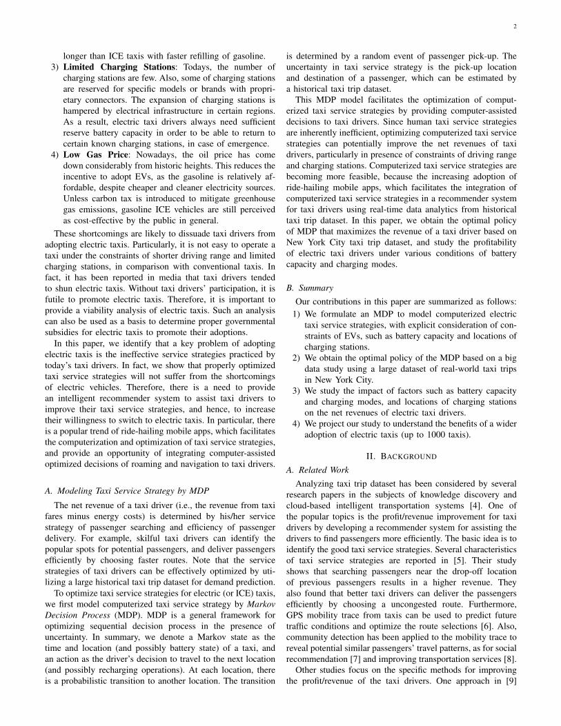
Observations: Figs. 9a-9b show the estimated net revenuesfor electric taxis under different battery capacities. The bluebars represent the net revenues using fast charging, while thered bars represent those using mode 3 charging. We observethat electric taxis equipped with 50 kWh battery can makecomparable net revenues with traditional ICE taxis using fastcharging for morning shifts. Note that in general smallerbatteries require more frequent recharging, which can reducerevenue. EVs with smaller batteries are cheaper. The netrevenue gap between using fast charging and mode 3 chargingis smaller when the battery capacity increases. The estimatednet revenue reaches USD$438 when battery capacity is above50 kWh. The net revenue is higher than that of ICE taxis

using optimized service strategies (i.e., USD$426 benchmark),because electricity cost is cheaper.

Figs. 9c-9d show the driving distances and energy consump-tions under different battery capacities. The blue borderedbar represent the driving distances using fast charging whilered bordered bars represent those using mode 3 charging.The green portions represent the amount of charging energyreceived from charging stations, while gray portions representthe amount from initial batteries. We observe that the totaldriving distance is around 242 kilometers without rechargingfor morning shifts. At night, the electric taxis are expectedto drive longer distances because of less traffic. The requiredenergy consumption without charging for morning shifts is43 kWh, which can be provided by 50 kWh battery (i.e.,45 kWh usable capacity) without recharging. For eveningshifts, the required energy consumption increases to 45.1 kWh.Therefore, electric taxis with 50 kWh battery are then requiredto recharge during shifts.

Ramifications: Optimizing taxi service strategies for elec-tric taxis can improve the profitability of taxi drivers. But theeffect depends on the battery capacity. With more capacity(e.g., 50 kWh, 70kWh), the taxi driver can earn comparablenet revenue with the one of ICE taxi using optimized servicestrategy. It is because that recharging will incur inefficiencyfor electric taxis with a low capacity battery.

C. Using Historical Data for PredictionSetting: The previous basic evaluation of net revenues is

based on MDP using the complete knowledge, which requiresknowing the pick-up demands and locations in a-priori man-ner. However, complete information is difficult to obtain in

10

1 2 3 4 5 6 7 8 9 10Num. of electric taxis in a junction

0.0

0.2

0.4

0.6

0.8

1.0

Rati

o

(a) Histogram of number oftaxis in a junction.

50 200 400 600 800 1000Number of electric taxis

200

250

300

350

400

450

500

Net

revenue (

USD

) Profit

0

50

100

150

200

250

300

Dis

tance

(km

)

Driving distance Delivery distance

(b) Estimated net revenues for multipleelectric taxis with 70 kWh battery ca-pacity.

0 200 400 600 800 1000275

300

325

350

375

400

425

Net

Revenue (

USD

) 70 kWhMon Tue Wed Thu Fir Sat Sun


30 kWh EVfast charging

0 200 400 600 800 1000

30 kWh EVmode 3 charging

(c) Estimated net revenues for multiple electric taxis over year 2013.

Fig. 11: Estimated net revenues for multiple electric taxis.

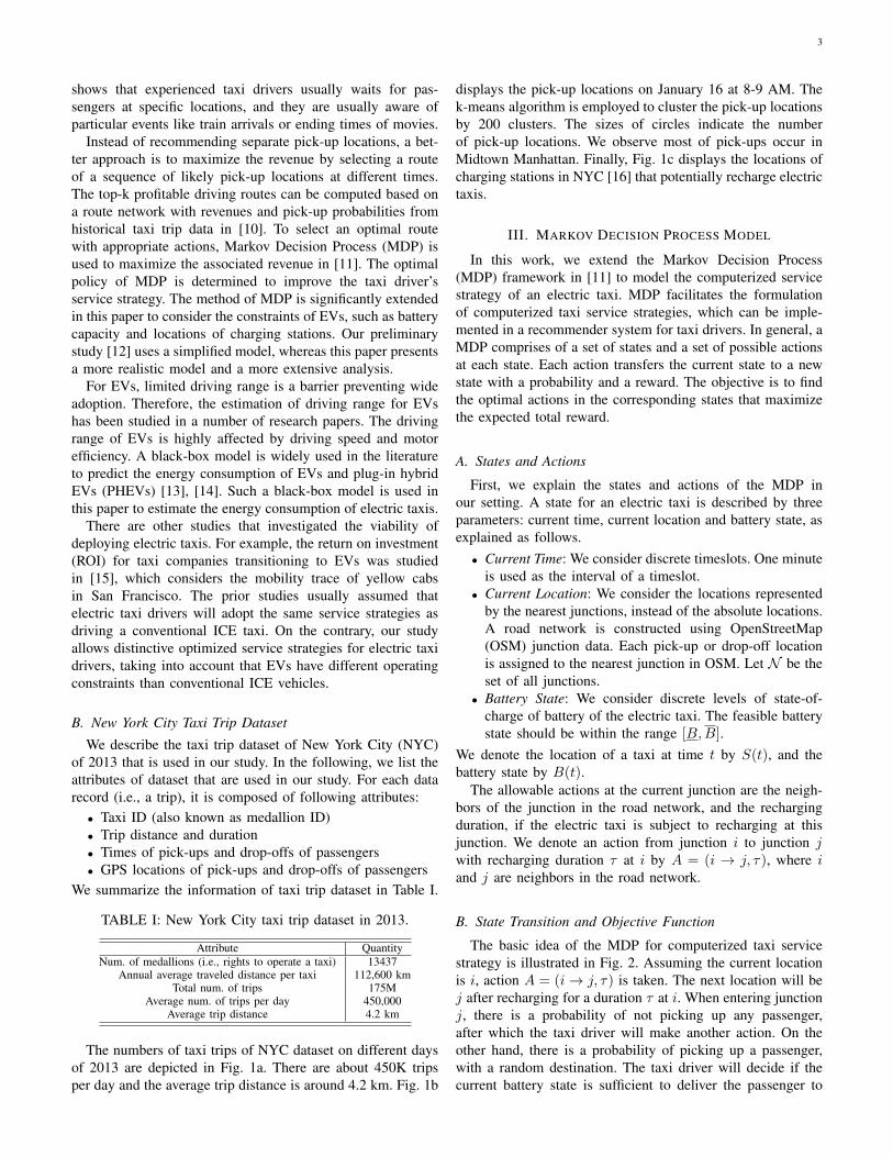
practice. A more practical approach is to use only historicaldata as training dataset for MDP, and then obtain an optimalpolicy as a heuristic for other days. In the following, we usethe optimal policy of MDP obtained from 6th January to 12thJanuary (i.e., the first week after 1st January) as training data.Then we employ the policy to all morning shifts in the yearin the evaluation.

Observations: Fig. 10 shows the estimated net revenueusing one-day training data on different days of a week.We observe that the highest net revenue occurs on Fridaywhile the lowest net revenue occurs on Sunday, becauseof more passengers on Fridays. The figures also show thebenchmark for ICE taxis using historical data (i.e., gray band).In particular, Fig. 10a shows the net revenue of 70 kWh batterycapacity using different dates in January as training data. Weobserve that the training data from 6th January performs thebest while training data from 8th January performs the worst.A taxi driver can receive 7.5% higher net revenue using 6thJanuary data.

Fig. 10c shows the net revenues with the 30 kWh batterycapacity using training data from 6th January. We observe that12% higher net revenue can be obtained using fast chargingthan using mode 3 charging. Electric taxis with 70 kWh batterycapacity can obtain 2.8% higher than 30 kWh battery capacityusing fast charging.

Ramifications: Using historical data for prediction, insteadof complete knowledge, will inevitably reduce the effective-ness. However, this creates a similar effect on ICE taxisthat also use historical data. Hence, optimizing taxi servicestrategies for electric taxis using historical data still achievescomparable net revenues as that of ICE taxis.

D. Multiple Electric Taxis

Setting: The optimal policy from MDP has been previouslyemployed in one single taxi. Next, we employ the optimalpolicy to multiple taxis. The idea is to allow multiple electrictaxis adopt the optimal policy from MDP, while ensuring thenumber of taxis being sent to each location is constrained.Otherwise, this leads to over-provision of taxis at certainlocations. This simple constraint allows us to decouple theindividual MDP decisions. Otherwise, considering a largecomplex problem will be intractable. In practice, we maydisplay the potential net revenue of each junction to the taxi

drivers. The junction will become less desirable, when thenumber of taxis currently present exceeds a certain threshold.Hence, they would not prefer to go to the junction.

We first empirically study the distribution of number of taxisat all the junctions over time from the dataset. We then set oflimit of the number of taxis at each junction according to themean number of taxis at each junction from the dataset. Tosatisfy the constraint, some electric taxis would need to followthe second-best decisions in the optimal policy. Each taxi stateis initialized by the junction and the time according to thedataset. The state of each taxi is tracked and the passengerpick-up probability P p

t (i) is recomputed using Eqn. (3). Weuse the optimal policy based on the data of 6th January.

Observations: Fig. 11a displays the histogram of numberof taxis in a junction. We observe that the number of taxis ineach junction is less than 7 by 99% of time. We set of limitof the number of taxis at each junction according to the meannumber of taxis at each junction from the dataset.

Fig. 11b shows the net revenues of different numbers ofelectric taxis using the optimal policy of MDP on 9 Jan. Weobserve that the net revenue drops to $USD 350 when 1000electric taxis use the optimal policy of MDP. The red barindicates the total driving distance of the taxis and blue barindicates the passenger delivery distance. We observe that thedelivery distance drops but the total driving distance remainsrelatively steady. This implies that the increase of roamingdistance is due to a lower passenger pick-up probability.Fig. 11c shows the average net revenue of multiple taxis overentire year of 2013. We observe that the highest net revenueoccurs on Fridays while the lowest occurs on Sundays. We alsoobserve that the net revenue is less affected by the number oftaxis when mode 3 charging is used. This is because that theelectric taxis require frequent recharging, which may result inless available taxis, and hence, a higher pick-up probability.

Ramifications: If the optimal policy of MDP is deployedup to 1000 electric taxis, then the net revenues will decrease,as a result of diminishing advantage of computerized servicestrategies. These 1000 taxi drivers can still earn as top 1.7%among traditional taxi drivers without computerized servicestrategies.

E. Considering Driving BehaviorSetting: Driving behavior plays an important role in energy

consumption of vehicles. Aggressive driving behavior results

11


300325350375400425450475

Net

revenue (

USD

)

ICE Benchmark

Mild

Normal

Aggressive

(a) Estimated net revenues ofdifferent driving behaviors usingmode 3 charging.


300325350375400425450475

Net

revenue (

USD

)

ICE Benchmark

Mild

Normal

Aggressive

(b) Estimated net revenues ofdifferent driving behaviors usingfast charging.


0

10

20

30

40

50

60

70

Tota

l Energ

y C

onsu

mpti

on

(kW

h)

Mild

Normal

Aggressive

(c) Energy consumption of dif-ferent driving behaviors usingmode 3 charging.


0

10

20

30

40

50

60

70

Tota

l Energ

y C

onsu

mpti

on

(kW

h)

From charging station

Original in battery

(d) Energy consumption of dif-ferent driving behaviors usingfast charging.

Fig. 12: Estimated net revenues and energy consumptions of different driving behaviors.

in more energy consumption. Furthermore, higher energyconsumption rate induces more frequent recharging of EVs,which reduces the net revenues of the taxi drivers. We studythree classes of driving behaviors: i) mild drivers (β = 0.8), ii)normal drivers (β = 1), and iii) aggressive drivers (β = 1.2).

Observations: Fig. 12 shows the estimated net revenues ofdifferent driving behaviors for morning shifts. Fig. 12a showsthe estimated net revenues of different driving behaviors usingmode 3 charging. Mild drivers can receive 14% higher net rev-enue than aggressive drivers when driving 30 kWh Leaf usingmode 3 charging. However, the net revenue is less affectedby different drivers when the battery capacity is sufficientlylarge to eliminate recharging during a shift. Fig. 12b shows theestimated net revenues using fast charging. We observe that thenet revenue is also less affected by different driving behaviorsbecause of shorter recharging duration. Fig. 12 shows theenergy consumption of different driving behaviors. We observethat aggressive drivers consume around 11 kWh more energythan mild drivers.

Ramifications: Although the aggressive drivers consumes20% more energy which only results in $USD2.2 differencefor morning shifts. The result shows that the driving behavioronly has a higher impact on the net revenue when the batterycapacity is insufficient to eliminate recharging during a shift.

F. Considering Different Gas Prices

Setting: To complete the study of viability of electric taxis,we provide a study of ICE taxis’ net revenue under differentgas prices. Note that the current gas price in USA is aroundUSD$2.5 per gallon, while the current gas price in China isaround 7.2 RMB per liter, which is equivalent to $4.5 USD pergallon. We analyze the outcomes of three different gas prices(i.e., $2.5 USD/G, $3.5 USD/G, $4.5 USD/G) considering theoptimal policy of MDP for an ICE taxi.

Observations: Fig. 13 compares the annual net revenues ofICE taxi under different gas prices, with that of electric taxisusing different charging options. We observe that the annualnet revenue with gas price $2.5 USD/G (i.e., the leftmost bar)is slightly higher (about USD$ 4000 higher) than that withgas price $4.5 USD/G. We also observe that the comparablenet revenue can be achieved by 30 kWh EV with fast chargingwhen gas price increases to $4.5 USD/G. However, the annualnet revenue of 30 kWh EV with mode 3 charging is muchlower (about 14% lower), even when the gas price is high.

ICE$2.5

USD/G

ICE$3.5

USD/G

ICE$4.5

USD/G

EV70 kWh

EV30 kWhfast chg.

EV30 kWh

mode 3 chg.

100

120

140

160

Annu

al n

et re

venu

e (U

SD th

ousa

nd)

Fig. 13: Annual net revenues under different gas prices.

Ramifications: We observe that when the gas price in-creases, ICE taxi becomes a less attractive option since its netrevenue decreases. The net revenue of 70 kWh EV is around3% higher than ICE taxi when gas price is $2.5 USD/G, whileit is around 6.6% higher than ICE taxi when gas price increasesto $4.5 USD/G.

G. Annual Evaluation of NYC Taxi Trip Dataset

1) Net Revenue Evaluation:Setting: We employ the optimal policy from 6th January to

different numbers of electric taxis and estimate the annual netrevenues. Fig. 15 shows the distribution of annual workinghours, we observe that the median annual working hour isaround 1800 hours, but many drivers work more than 4300hours, equivalent to working almost 12 hours a day. Therefore,we consider taxi drivers working every morning shift (i.e.,4380 working hours) to estimate their net revenues.

0 1000 2000 3000 4000Annual work time (hr)

0

200

400

600

800

1000

1200

Num

ber

Median

20 40 60 80 100 120 140 160Annual net revenue (USD thousand)

1 MDP EV driver

1 MDP ICE driver

1000 MDP drivers in 70kWh EV (.07%)

1000 MDP drivers in 30kWh EVfast charging (.15%)

1000 MDP drivers in 30kWh EVmode 3 charging (.4%)

Fig. 15: Annual working hours and estimated net revenues oftaxi drivers in 2013.

12

0 50 100 150 200 250 300 350Day of year 2013

20406080

100120140160180200220

Daily

energ

yco

nsu

mpti

on (

MW

h)

70kWh EV

30kWh EVmode 3 charging

ICE

(a) Daily energy consumption ofmorning shifts.

0 50 100 150 200 250 300 350Day of year 2013

70kWh EV

30kWh EVmode 3 charging

ICE

(b) Daily energy consumptionof night shifts.


0

20

40

60

80

100

120

140

Annual energ

y c

onsu

mpti

on

(BW

h)

30 kWh with mode 3 charging

70 kWh

ICE

(c) Annual energy consumption ofdifferent numbers of electric taxis.


0

5

10

15

20

25

30

35

40

Annual C

O2 e

mis

sion

(k m

etr

ic t

ons)

30 kWh with mode 3 charging

70 kWh

ICE

(d) Annual CO2 emission of dif-ferent numbers of electric taxis.

Fig. 14: Daily and annual energy consumption and CO2 emission.

Observations: The right figure in Fig. 15 shows the esti-mated net revenues of different taxi drivers using the optimalpolicy of MDP. There are some observations:• The case of one electric taxi driver using the optimal

policy of MDP can earn 3% higher than that of one ICEtaxi driver.

• The average net revenue of case of 1000 electric taxiswith 70 kWh battery is ranked top 0.07% among tradi-tional taxi drivers without computerized service strategy.

• The average net revenue of case of 1000 electric taxiswith 30 kWh battery using mode 3 charging is ranked top0.4% among traditional taxi drivers without computerizedservice strategy.

The results shows that the optimal policy of MDP can enableelectric taxi drivers to make comparable revenues as traditionaltaxi drivers.

2) Carbon Emission Evaluation:Setting: Besides of net revenues as economic motivation,

an important benefit is the reduction of carbon emission byswitching from ICE taxis to electric taxis. Although electrictaxis do not produce tailpipe emissions, the electricity gridto recharge the battery may still produce emissions. In thissection, we estimate the CO2 emission of electric taxis, ascompared with ICE taxis, with computerized service strategyoptimization. The CO2 emission factors of electricity andgasoline are obtained from eGrid of Long Island [2]:• Emission factor of electricity: 0.7007 kg/kWh• Emission factor of gasoline: 2.348 kg/literObservations: We consider taxis working in all shifts.

Fig. 14a shows the daily energy consumption of 1000 taxisfor morning shifts, while Fig. 14b shows the daily energyconsumption for night shifts. We use miles per gallon gasolineequivalent to convert the consumed gasoline to kWh (i.e., 1gallon of gasoline equals to 33.7 kWh). Fig. 14c shows theannual energy consumption of different numbers of electrictaxis. We observe that ICE taxis consume around 4 times moreenergy than electric taxis. Fig. 14d shows the correspondingCO2 emissions of different numbers of electric taxis. Weobserve that up to 15 thousand metric tons CO2 (equal to 1560home’s energy use for one year) can be saved by replacing1000 ICE taxis by electric taxis.

VI. CONCLUSION

In this paper, we employ Markov Decision Process tomodel computerized taxi service strategy and optimize the

strategy for taxi drivers considering electric taxi operationalconstraints. We evaluate the effectiveness of the optimal policyof Markov Decision Process using a big data study of real-world taxi trips in New York City. The optimal policy canbe implemented in an intelligent recommender system fortaxi drivers. This becomes more viable especially due to theadvent of autonomous vehicles. Our evaluation shows thatcomputerized service strategy optimization allows electric taxidrivers to earn comparable net revenues as ICE drivers, whoalso employ computerized service strategy optimization, withat least 50 kWh battery capacity. Hence, this sheds light onthe viability of electric taxis.

REFERENCES

[1] NYC Taxi & Limousine Commission. (2014) Taxicab Fact Book.[2] USA Environmental Protection Agency. (2017) Greenhouse Gases

Equivalences Calculator.[3] South China Morning Post. (2017) After Hong Kong Failure, China’s

BYD Joins Singapore Launch.[4] E. Wilhelm, J. Siegel, S. Mayer, L. Sadamori, S. Dsouza, C.-K. Chau,

and S. Sarma, “Cloudthink: A scalable secure platform for mirroringtransportation systems in the cloud,” Transport, vol. 30, no. 3, 2015.

[5] D. Zhang, L. Sun, B. Li, C. Chen, G. Pan, S. Li, and Z. Wu,“Understanding Taxi Service Strategies From Taxi GPS Traces,” IEEETrans. Intell. Transp. Syst., vol. 16, pp. 123–135, 2015.

[6] S. Liu, Y. Yue, and R. Krishnan, “Non-Myopic Adaptive Route Planningin Uncertain Congestion Environments,” IEEE Trans. Knowledge andData Engineering, vol. 27, pp. 2438 – 2451, 2015.

[7] S. Liu and S. Wang, “Trajectory Community Discovery and Recommen-dation by Multi-Source Diffusion Modeling,” IEEE Trans. Knowledgeand Data Engineering, vol. 29, pp. 898–911, 2017.

[8] J. Zhao, Q. Qu, F. Zhang, C. Xu, and S. Liu, “Spatio-Temporal Analysisof Passenger Travel Patterns in Massive Smart Card Data,” IEEE Trans.Intell. Transp. Syst., vol. 18, pp. 3135–3146, 2017.

[9] J. Yuan, Y. Zheng, L. Zhang, X. Xie, and G. Sun, “Where to Find MyNext Passenger?” in ACM Int. Conf. Ubiquitous Computing (UbiComp),2011.

[10] M. Qu, H. Zhu, J. Liu, G. Liu, and H. Xiong, “A Cost-effectiveRecommender System for Taxi Drivers,” in ACM Int. Conf. KnowledgeDiscovery and Data Mining (SIGKDD), 2014.

[11] H. Rong, X. Zhou, C. Yang, Z. Shafiq, and A. Liu, “The Rich and thePoor: A Markov Decision Process Approach to Optimizing Taxi DriverRevenue Efficiency,” in ACM Int. Conf. Information and KnowledgeManagement (CIKM), 2016.

[12] C.-M. Tseng and C.-K. Chau, “Viability Analysis of Electric Taxis UsingNew York City Dataset ,” in ACM Workshop on Electric Vehicle Systems,Data and Applications (EVSys), 2017.

[13] ——, “Personalized Prediction of Vehicle Energy Consumption basedon Participatory Sensing,” IEEE Trans. Intell. Transp. Syst., vol. 18,no. 11, pp. 3103–3113, 2017.

[14] C.-K. Chau, K. Elbassioni, and C.-M. Tseng, “Drive Mode Optimizationand Path Planning for Plug-in Hybrid Electric Vehicles,” IEEE Trans.Intell. Transp. Syst., vol. 18, no. 12, pp. 3421–3432, 2017.

13

[15] T. Carpenter, A. R. Curtis, and S. Keshav, “The Return On Investmentfor Taxi Companies Transitioning to Electric Cehicles - A Case Studyin San Francisco,” Journal Transportation, vol. 41, pp. 785–818, 2014.

[16] New York government. (2017) Electric Vehicle Charging Stations inNew York.

[17] A. Furieri. (2017) The Gaia-SINS federated projects.[18] FleetCarma. (2014) Real-world range ramifications: heating and air

condition.[19] C. Bingham, C. Walsh, and S. Carroll, “Impact of Driving Characteristics

on Electric Vehicle Energy Consumption and Range,” IET IntelligentTransport Systems, vol. 6, no. 1, pp. 29–35, 2012.

[20] L. Feng and B. Chen, “Study the Impact of Driver’s Behavior on theEnergy Efficiency of Hybrid Electric Vehicles,” in ASME Intl. DesignEngineering Technical Conference, 2013.

ACKNOWLEDGMENT

The authors would like to thank Srinivasan Keshav andSgouris Sgouridis for helpful suggestions and discussions.

improving viability of electric taxis by taxi service strategy optimization: a big … · index...

Documents