improving the plausibility of the missing at random

Improving the plausibility of the

missing at random assumption in

the 1958 British birth cohort:

A pragmatic data driven

approach

CLS working paper number 2020/6

By T. Mostafa, M. Narayanan, B. Pongiglione,

B. Dodgeon, A. Goodman, R.J. Silverwood

and G.B. Ploubidis

Corresponding author

George B. Ploubidis

UCL Centre for Longitudinal Studies

[email protected]

This working paper was first published in April 2020 by the UCL Centre for Longitudinal

Studies.

UCL Institute of Education

University College London

20 Bedford Way

London WC1H 0AL

www.cls.ucl.ac.uk

The UCL Centre for Longitudinal Studies (CLS) is an Economic and Social Research

Council (ESRC) Resource Centre based at the UCL Institution of Education (IOE), University

College London. It manages four internationally-renowned cohort studies: the 1958 National

Child Development Study, the 1970 British Cohort Study, Next Steps, and the Millennium

Cohort Study. For more information, visit www.cls.ucl.ac.uk.

This document is available in alternative formats. Please contact the

Centre for Longitudinal Studies.

Tel: +44 (0)20 7612 6875

Email: [email protected]

http://www.cls.ucl.ac.uk/

http://www.cls.ucl.ac.uk/

mailto:[email protected]

Disclaimer

This working paper has not been subject to peer review.

CLS working papers often represent preliminary work and are circulated to

encourage discussion. Citation of such a paper should account for its provisional

character. A revised version may be available directly from the author.

Any opinions expressed here are those of the author(s) and not those of the UCL

Centre for Longitudinal Studies (CLS), the UCL Institute of Education, University

College London, or the Economic and Social Research Council.

How to cite this paper

Mostafa, T., Narayanan, M., Pongiglione, B., Dodgeon, B., Goodman, A.,

Silverwood, R.J., and Ploubidis, G.B. (2020) Improving the plausibility of the missing

at random assumption in the 1958 British birth cohort: A pragmatic data driven

approach, CLS Working Paper 2020/6. London: UCL Centre for Longitudinal

Studies.

A peer-reviewed version of this paper can be found in the Journal of Clinical

Epidemiology (Volume 136, August 2021, pages 44-54): https://doi.org/10.1016/

j.jclinepi.2021.02.019

https://doi.org/10.1016/j.jclinepi.2021.02.019

1

ABSTRACT

Making the Missing At Random (MAR) assumption more plausible has implications for

missing data analysis. We capitalise on the rich data of the National Child

Development Study (NCDS - 1958 British birth cohort) and implement a systematic

data-driven approach to identify predictors of non-response from the 11 sweeps (birth

to age 55) of the NCDS (n = 17,415). We employed parametric regressions and the

Least Absolute Shrinkage and Selection Operator for variable selection.

Disadvantaged socio-economic background in childhood, worse mental health and

lower cognitive ability in early life, and lack of civic and social participation in adulthood

were consistently associated with non-response. Using this information, we were able

to restore the composition of the NCDS samples at age 50 and age 55 to be

representative of the study’s target population, using external benchmarks, and

according to a number of characteristics captured within the original birth sample. We

have shown that capitalising on the richness of NCDS allowed us to identify predictors

of non-response that improve the plausibility of the MAR assumption. These variables

can be straightforwardly used in analyses with principled methods to reduce bias due

to missing data and have the strong potential to restore sample representativeness.

KEYWORDS

Attrition; Cohort studies; Longitudinal data; Missing data; Multiple imputation; National

Child Development Study; Non-response.

2

INTRODUCTION

Non-response is unavoidable in longitudinal surveys. The consequences are smaller

samples due to attrition, lower statistical power and decreased representativeness

compared to the originally intended target population. With some exceptions where

complete case analysis is valid(Bartlett, Carpenter, Tilling, & Vansteelandt, 2014;

Daniel, Kenward, Cousens, & De Stavola, 2012; Hughes, Heron, Tilling, & Sterne,

2019), in the majority of analyses of longitudinal data unbiased estimates cannot be

obtained without formally addressing the implications of selection bias due to

incompleteness(Carpenter & Kenward, 2012; Sterne et al., 2009). There is a broad

interdisciplinary consensus that missing data should be dealt with using principled

approaches and it has recently been argued that “complete-case analysis should be

used with the same caution we ascribe to unadjusted estimates, as its validity relies

on strong, often unrealistic assumptions” (Perkins et al., 2018).

Rubin described three missing data generating mechanisms: i) Missing Completely

At Random (MCAR); ii) Missing At Random (MAR); iii) Missing Not At Random

(MNAR) (Hughes et al., 2019; Little & Rubin, 1989, 2002). MCAR implies that the

probability of non-response is not due to any variable (measured or unmeasured)

being associated with the variables in the substantive model of interest, or that there

are no systematic differences between the observed and missing data. MCAR is

partially testable since we can find out whether variables available in our data are

associated with non-response or other forms of missingness. MAR implies that

systematic differences between the missing values and the observed values can be

explained by observed data, or that given the observed/available data, the reasons for

missingness do not depend on unobservables. With some exceptions for specific

missing data patterns (Mohan, Pearl, & Tian, 2013; Robins & Gill, 1997) the MAR

3

assumption is untestable (Molenberghs, Beunckens, Sotto, & Kenward, 2008). The

third mechanism - MNAR - implies that that the available data are insufficient to explain

variation in the probability of missing data. MNAR is also untestable and methods to

deal with this type of missing data generating mechanism rely heavily on further –

usually distributional - assumptions (Muthen, Asparouhov, Hunter, & Leuchter, 2011).

Contextualising the 1958 British National Child Development Study (NCDS) within

Rubin’s framework, we know that the missing data generating mechanism is not

MCAR as previous work (Atherton, Fuller, Shepherd, Strachan, & Power, 2008;

Hawkes & Plewis, 2006) has shown that various variables are associated with non-

response. In practice, as is expected to be the case in the vast majority of longitudinal

surveys, the missing data generating mechanism in most analyses employing NCDS

is MAR or MNAR. Since both are largely untestable and considering that flexible

solutions and software are available that return valid estimates assuming MAR, a

pertinent question is how we can make MAR more plausible. Principled approaches

that deal with missingness, such as Multiple Imputation (MI), Full Information

Maximum Likelihood (FIML) and Inverse Probability Weighting (IPW) assume MAR

and thus are more likely to produce unbiased estimates if careful steps have been

taken to maximise its plausibility (C. K. Enders, 2001; Little & Rubin, 1989, 2002;

Perkins et al., 2018; Wooldridge, 2007). In the missing data methodology literature it

is accepted that making MAR more plausible can be achieved by employing “auxiliary”

– not in the substantive model of interest - variables, either in the imputation phase of

Multiple Imputation (MI), directly in Full Information Maximum Likelihood (FIML)

analysis, or in the derivation of non-response weights(C. E. Enders, 2010; S. R.

Seaman & White, 2011). Effective auxiliary variables are thought to be variables

associated both with non-response and the substantive outcome of interest, as well

4

as variables strongly associated with the substantive outcome of interest only, since

the expectation is that if so, they will also be associated with its missing

values(Carpenter & Kenward, 2012). There is disagreement as to which variables

associated only with non-response/missingness constitute effective auxiliary

variables, with some authors arguing in favour of their inclusion(Collins, Schafer, &

Kam, 2001; C. E. Enders, 2010) and others against(Carpenter & Kenward, 2012).

We capitalise on the rich data available in NCDS and present a systematic data-

driven approach to identify predictors of non-response in all available sweeps. This

has the potential to make the MAR assumption more plausible in applied analyses of

NCDS data as it will allow researchers to identify the subset of predictors of non-

response that are also associated with their substantive outcome of interest and use

these as auxiliary variables. We also investigate whether by using information

available in NCDS we are able to restore sample representatives despite attrition.

METHODS

Data

The NCDS(Power & Elliott, 2006) is one of the oldest and most well-characterised

birth cohort studies, with 10 major follow-ups since birth. The initial sample of 17,415

individuals – consisting of all babies born in Great Britain in a single week in 1958 –

was supplemented with migrants at ages 7, 11 and 16. The most recent follow-up was

at age 55, with high quality prospective data on social, biological, physical, and

psychological phenotypes available at every sweep. In 2002, when respondents were

44-45 years old, a biomedical survey was conducted in more than 9,000 respondents.

We used for the Office for National Statistics Annual Population Survey(Division, 2004

5

- 2017) to obtain estimates of the population distribution of key demographic

characteristics for those born in 1958 and residing in Great Britain in 2008.

Exposures - predictors of non-response

NCDS datasets from the sweeps up to age 50 deposited in the UK Data Service

include a total of 17,412 variables that could potentially be used as predictors of non-

response. However, many of these variables are so called “routed”, where only cohort

members that gave a specific response to a previous question are asked these

subsequent questions. For example, variables with information on the presence of

specific chronic illnesses are routed on a previous question about the presence of any

chronic illness and only those with a chronic illness respond to the subsequent

questions. To avoid sample selection the majority of “routed” variables were excluded

from the analysis. Exceptions included variables related to occupational social class

and employment status. We also excluded binary variables with prevalence less than

1% and variables with item non-response > 50%. We did so as low prevalent

categories in binary variables that cannot be collapsed with others would be

problematic in the multivariable regression models we employ for variable selection.

Similarly, variables with >50% of item non-response in addition to unit non-response

would, in combination with missingness in the other predictors of non-response,

reduce the available data to <10% in later sweeps. Summary scores were calculated

for all scales, further reducing the number of eligible variables. In sweeps where more

than one scale was available that taps into the same construct, we included in the

analysis the one available in most sweeps. Finally, variables that reflect questions

used to derive summary measures such as household income, employment status

and educational qualifications were not selected as summaries were available. This

6

resulted in 587 variables that met the criteria for inclusion in the analysis. They cover

all domains captured by the NCDS (Power & Elliott, 2006), including indicators of

socio-economic position, demographic characteristics, health, health behaviour,

educational attainment, cognitive ability, personality traits, disability, relationships,

social and political participation, biomarkers and others. In addition to these variables

we calculated a summary variable that captures, for each sweep separately, whether

or not cohort members participated in all previous NCDS sweeps.

Outcomes

We used binary variables indicating non-response for each sweep of NCDS from age

7 onwards. We defined non-response as participants who did not take part in the

survey, either because of refusal, the survey team not been being able to establish

contact, or because contact was not attempted. We did not consider as non-response

participants that have died or emigrated since our aim was to identify predictors of

non-response and not of mortality or emigration. We view missing data analysis as an

attempt to restore sample representativeness with respect to a well-defined target

population. The target population of NCDS, and any other longitudinal survey, is

dynamic, as changes occur for example due to mortality. Considering that the NCDS

mortality rate is representative of the population (Figure 1 and Table S1), the target

population in each sweep of NCDS needs to be adjusted accordingly to reflect these

changes. With the exception of modelling mortality as an outcome of interest, including

participants that have died in any form of missing data analysis within NCDS would be

the equivalent of generalising estimates to a non-existent (immortal) target population.

7

Figure 1. NCDS (England and Wales sample) & Office for National Statistics standardised mortality rate for England and Wales

8

Analytic strategy

In order to identify the important predictors of sweep-specific non-response we

employed a three-stage analytic strategy using the identified 587 eligible variables as

input. We opted for a three-stage approach since the majority of the 587 potential

predictors of non-response were not complete and imputing all these variables

simultaneously was not feasible. Non-response at each sweep was analysed

separately throughout the three-stage procedure. The three-stage approach can be

summarised as follows for non-response at sweep t:

• Stage 1: Complete case univariable modified Poisson regressions(Zou, 2004)

of non-response at sweep t on each potential predictor of non-response at

sweep 0, …, sweep t – 1. Retain predictors with p < 0.05.

• Stage 2: Complete case multivariable modified Poisson regressions of non-

response at sweep t on all retained predictors at sweep 0, then separately on

all retained predictors at sweep 1, etc., up to all retained predictors at sweep t

– 1. Retain predictors with p < 0.05.

• Stage 3: MI using all retained variables plus non-response at sweep t in the

imputation model. MI multivariable modified Poisson regressions for all retained

predictors at sweep 0, …, sweep t – 1, adjusted for predictors at all previous

(but not subsequent) sweeps. Retain predictors with p < 0.001.

Stage 3 allowed us to compare predictors of non-response from all stages of the life

course and identify the set that has the potential to maximise the probability of the

MAR assumption for a given NCDS sweep. Estimating a series of models in which

predictors of non-response at a given sweep were adjusted for predictors at previous

(but not subsequent) sweeps preserves the temporal sequence of the life course

9

information available in NCDS while avoiding over-adjustment from conditioning on

variables on the causal pathway between a given predictor and non-response. When

considering non-response at sweep t the number of models estimated was thus t (one

for each sweep between 0 and t – 1). So, for example, when considering non-response

at sweep 6 (age 42), six models were estimated. The first of these models predicted

non-response at age 42 from variables at sweep 0 (birth) that were retained after

Stages 1 and 2.

This allowed us to capture the association between variables available at birth and

non-response at age 42, without adjusting for variables from subsequent sweeps (age

7 onwards) that lie on the causal pathway between our exposures and outcome. The

final of these models predicted non-response at age 42 from variables at sweep 5 (age

33) that were retained after Stages 1 and 2, while also adjusting for variables at

sweeps between 0 and 4 that had been retained after Stages 1 and 2.

In addition to protecting from over-adjustment, this approach ensures the richest

adjustment, since from the results of Stage 2 we know that these are all the variables

from the 587 included in the analysis potentially associated with non-response at a

given sweep. We note that this approach introduces a causal structure based on

temporal sequencing of predictors of non-response as they appear in the various

sweeps of NCDS. The rationale that underlies our decision is influenced by the fact

that variables from early sweeps are relatively “complete” and are therefore more

suitable candidates as auxiliary variables, considering that our ultimate goal is to

inform applied analyses in NCDS.

We relied on P-values within our regression-based approach. We could instead have

considered the magnitude of the association, but this is scale dependent, which is of

particular concern for continuous predictors of non-response. For categorical

10

predictors, the magnitude of the risk ratio for a given category would be dependent on

the choice of baseline category and, in addition, for binary or categorical predictors,

spuriously large (but imprecisely estimated) risk ratios could result from very low

prevalence categories, leading to false positive variable selection.

The above three-stage procedure was repeated considering non-response at each

sweep in turn. We defined “consistent” predictors of non-response to be variables

identified at Stage 3 as predictors of non-response at 50% or more of the sweeps in

which they were eligible to be considered. For example, a variable from sweep 3 (age

16) could potentially be associated with non-response in seven subsequent sweeps.

If such a predictor was associated with non-response in 4 or more subsequent sweeps

it was selected as a consistent predictor of non-response.

In order to investigate whether the predictors of non-response identified at Stage 3

have the potential to restore sample representativeness in NCDS despite attrition, we

compared estimates from NCDS participants at age 50 with the known population

distribution of educational attainment and marital status derived from the Office for

National Statistics Annual Population Survey in 2008. Within this analysis we

compared the relative effectiveness of the identified predictors of non-response

compared to variables associated with education and marital status. We also

investigated whether the original distributions of paternal social class at birth and

cognitive ability at age 7 could be replicated using data from only respondents at age

55 (i.e. disregarding data from non-respondents at age 55).

Statistical modelling

We modelled non-response with a log binomial model with robust standard errors

(modified Poisson regression) that returns risk ratios as non-response after age 23

11

becomes more common (>20%) to avoid bias due to non-collapsibility of the odds ratio

(M. Pang, J. S. Kaufman, & R. W. Platt, 2016; Menglan Pang, Jay S Kaufman, &

Robert W Platt, 2016). At Stage 2 we also employed the Least Absolute Shrinkage

and Selection Operator (LASSO)(Hastie & Qian, 2014) as a robustness check for

variable selection. Group LASSO was used to appropriately consider categorical

variables within the procedure (Yuan & Lin, 2006). Considering that the majority of the

587 variables are not complete, we did not employ the LASSO or any other machine

learning algorithm for variable selection at Stage 3. To the best of our knowledge, we

are not aware of existing theory, let alone software, that allows the combination of MI

with the LASSO or other machine learning approaches. We have therefore opted to

use the LASSO as a form of sensitivity analysis at Stage 2 where missingness is less

of an issue since variables are allowed to compete with others from the same sweep.

However, a Stage 3 sensitivity analysis was also conducted using the variables

selected using the LASSO at Stage 2 but using log-binomial modelling as in the

primary analysis. The LASSO procedure was undertaken using logistic regression as

log-binomial models were not available, and the optimal set of variables was selected

according to the minimum cross-validation error. As results were very similar with log

binomial regressions, we present these (LASSO estimates for sweeps 1 and 2 are

presented in the Web Appendix, and for all other sweeps are available from the

corresponding author).

As the variables included in the analysis at Stage 3 were subject to varying degrees

of missingness, MI was used to impute missing values in the predictors of non-

response We employed MI with chained equations (Azur, Stuart, Frangakis, & Leaf,

2011; Harel et al., 2018; White, Royston, & Wood, 2011) and generated 50 datasets

with imputed values using the previously identified from Stage 2 sweep specific

12

predictors of non-response in the imputation phase. MI was carried out for each

outcome (i.e. non-response at each sweep) separately as different predictors for non-

response at each sweep had been identified from Stage 2. All analyses were

conducted in Stata 14 – 16 and gglasso in R.

Table 1. Participation in the 1958 British National Child Development Study from birth to 55 years

Total cohort Dead Emigrants

Eligible sample Participants

(% of eligible sample)

Birth - 1958 17638 0 0 17638 17415 98.7 Age 7 - 1965 18016a 821 475 16720 15425 92.3 Age 11 - 1969 18287a 840 701 16746 15337 91.6 Age 16 - 1974 18558a 873 799 16886 14654 86.8 Age 23 - 1981 18558 960 1196 16402 12357 75.3 Age 33 - 1991 18558 1049 1335 16174 11469 70.9 Age 42 - 2000 18558 1199 1268 16091 11419 71.0 Age 44 - 2002 18558 1321 1234 16003 9377 58.6 Age 46 - 2004 18558 1323 1272 15963 9534 59.7 Age 50 - 2008 18558 1459 1293 15806 9790 61.9 Age 55 - 2013 18558 1659 1286 15613 9137 58.5

a The original sample was supplemented by migrants born in 1958

RESULTS

Non-response in NCDS

In Table 1 we present descriptive statistics of participation in the NCDS from birth to

55 years. As expected, participation drops with time, with notable sample size

reductions being at age 23, the first sweep where the cohort members were

responsible for participating in the survey instead of their parents, as well as at age 44

for the NCDS biomedical sweep. From the 17,415 cohort members that participated

in the first sweep, 4497 (25.8%) have participated in all 11 sweeps; of all 18,558 cohort

members, 11,232 (60.5%) of cohort members have taken part in 7 or more sweeps of

NCDS.

13

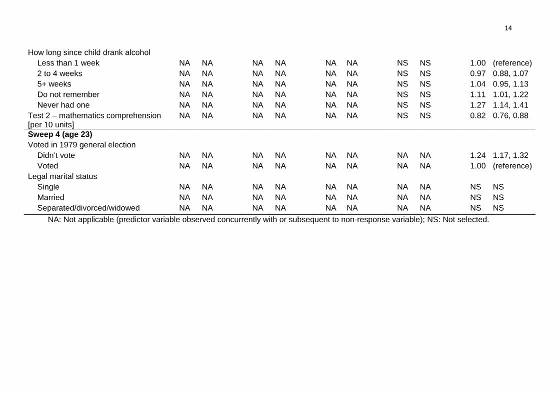
Table 2. Estimated risk ratios and 95% confidence intervals for consistent predictors (selected in at least 50% of possible sweeps) of non-response at sweeps 1-5 (ages 7-33) in the 1958 British National Child Development Study.

Sweep 1 (age 7) Sweep 2 (age 11) Sweep 3 (age 16)

Sweep 4 (age 23) Sweep 5 (age 33)

RR 95% CI RR 95% CI RR 95% CI RR 95% CI RR 95% CI

Non-response at previous sweep(s)

Complete response NA NA 1.00 (reference) 1.00 (reference) 1.00 (reference) 1.00 (reference)

Incomplete response NA NA 5.76 5.28, 6.28 2.84 2.62, 3.06 2.10 1.99, 2.22 2.33 2.21, 2.46

Sweep 0 (age 0)

Number of persons per room [per person] 1.10 1.05, 1.16 NS NS NS NS 1.11 1.08, 1.14 1.11 1.09, 1.13

Sex of child

Male NS NS NS NS NS NS 1.18 1.12, 1.25 1.22 1.16, 1.28

Female NS NS NS NS NS NS 1.00 (reference) 1.00 (reference)

Social class of mother’s husband

I 1.00 (reference) NS NS NS NS 1.00 (reference) 1.00 (reference)

II 0.66 0.51, 0.84 NS NS NS NS 1.01 0.85, 1.21 1.06 0.90, 1.24

III non-manual 0.65 0.49, 0.86 NS NS NS NS 0.91 0.75, 1.10 1.05 0.89, 1.25

III manual 0.59 0.47, 0.73 NS NS NS NS 1.13 0.96, 1.32 1.21 1.04, 1.40

IV 0.72 0.57, 0.92 NS NS NS NS 1.14 0.96, 1.36 1.30 1.11, 1.52

V 0.80 0.62, 1.02 NS NS NS NS 1.46 1.23, 1.73 1.72 1.47, 2.00

Sweep 1 (age 7)

Cognitive ability summary [per unit] NA NA 0.85 0.80, 0.91 NS NS 0.86 0.83, 0.89 0.87 0.84, 0.89

Social problems (alcoholism etc.) [per problem]

NA NA NS NS NS NS NS NS 1.10 1.07, 1.13

Sweep 2 (age 11)

Cognitive ability summary [per 10 units] NA NA NA NA NS NS 0.91 0.88, 0.94 0.89 0.87, 0.92

Sweep 3 (age 16)

Conduct problems [per unit] NA NA NA NA NA NA 1.10 1.07, 1.13 NS NS

14

How long since child drank alcohol

Less than 1 week NA NA NA NA NA NA NS NS 1.00 (reference)

2 to 4 weeks NA NA NA NA NA NA NS NS 0.97 0.88, 1.07

5+ weeks NA NA NA NA NA NA NS NS 1.04 0.95, 1.13

Do not remember NA NA NA NA NA NA NS NS 1.11 1.01, 1.22

Never had one NA NA NA NA NA NA NS NS 1.27 1.14, 1.41

Test 2 – mathematics comprehension [per 10 units]

NA NA NA NA NA NA NS NS 0.82 0.76, 0.88

Sweep 4 (age 23)

Voted in 1979 general election

Didn’t vote NA NA NA NA NA NA NA NA 1.24 1.17, 1.32

Voted NA NA NA NA NA NA NA NA 1.00 (reference)

Legal marital status

Single NA NA NA NA NA NA NA NA NS NS

Married NA NA NA NA NA NA NA NA NS NS

Separated/divorced/widowed NA NA NA NA NA NA NA NA NS NS

NA: Not applicable (predictor variable observed concurrently with or subsequent to non-response variable); NS: Not selected.

15

Predictors of non-response

In the Web Appendix we present the results of the variable selection process we

employed to identify predictors of non-response for all NCDS sweeps (Figures S1 –

S10 and Tables S2-S11). In Tables 2 and 3 we present risk ratios and 95% confidence

intervals from 20 “consistent” predictors of non-response across sweeps of NCDS.

Females and cohort members that took part in all previous sweeps were more likely

to participate in NCDS. Disadvantaged social class at birth and number of people per

room were associated with non-response in most adult sweeps, but not – or even

inversely associated - until age 23, indicating that parents from less advantaged socio-

economic backgrounds were more likely to participate in the survey, but their offspring

were more likely to drop out. Cognitive ability at ages 7 and 11 was consistently

associated with survey participation, whereas conduct problems at age 16 were

consistently associated with non-response. In adult sweeps, a systematic pattern

emerged, with social participation, voting and marriage/cohabitation being associated

with participation in NCDS. Other predictors associated with survey participation

included early life social problems, lower maths comprehension and never having

drank alcohol by age 16. Using the LASSO rather than log-binomial regression at

Stage 2 resulted in the selection of a greater number of variables (Table S12).

However, once the log-binomial Stage 3 was conducted using the LASSO-selected

Stage 2 variables, the resultant final selection of variables differed little from that in the

primary analysis (Tables S13 and S14 vs. S2 and S3).

16

Table 3. Estimated risk ratios and 95% confidence intervals for consistent predictors (selected in at least 50% of possible sweeps) of non-response at sweeps 6-9 (ages 42-55) in the 1958 British National Child Development Study.

Sweep 6 (age 42)

Biomedical sweep (age 44)

Sweep 7 (age 46)

Sweep 8 (age 50)

Sweep 9 (age 55)


Non-response at previous sweeps

Complete response 1.00 (reference) 1.00 (reference) 1.00 (reference) 1.00 (reference) 1.00 (reference)

Incomplete response 3.83 3.57, 4.11 3.37 3.17, 3.58 7.17 6.53, 7.88 6.28 5.71, 6.91 5.93 5.39, 6.54

Sweep 0 (age 0)

Number of persons per room [per person]

1.11 1.09, 1.13 1.08 1.07, 1.10 1.08 1.06, 1.10 1.07 1.05, 1.09 1.06 1.04, 1.08

Sex of child

Male 1.19 1.13, 1.25 1.07 1.03, 1.11 1.14 1.10, 1.19 1.11 1.07, 1.46 1.13 1.09, 1.18

Female 1.00 (reference) 1.00 (reference) 1.00 (reference) 1.00 (reference) 1.00 (reference)


I 1.00 (reference) 1.00 (reference) 1.00 (reference) 1.00 (reference) 1.00 (reference)

II 0.94 0.80, 1.11 1.08 0.95, 1.23 1.09 0.96, 1.25 0.98 0.86, 1.12 1.00 (reference)

III non-manual 1.02 0.86, 1.20 1.14 1.00, 1.30 1.13 0.99, 1.29 1.05 0.92, 1.20 1.11 1.01, 1.22

III manual 1.18 1.02, 1.36 1.25 1.12, 1.40 1.27 1.13, 1.43 1.18 1.05, 1.32 1.35 1.26, 1.43

IV 1.22 1.05, 1.43 1.32 1.16, 1.49 1.34 1.18, 1.52 1.27 1.12, 1.43 1.41 1.31, 1.53

V 1.51 1.30, 1.77 1.55 1.38, 1.75 1.62 1.43, 1.83 1.45 1.28, 1.63 1.69 1.57, 1.82

Sweep 1 (age 7)

Cognitive ability summary [per unit] 0.83 0.80, 0.85 0.85 0.83, 0.87 0.83 0.81, 0.85 0.84 0.82, 0.86 0.82 0.80, 0.84


NS NS 1.04 1.02, 1.06 1.03 1.01, 1.05 1.07 1.04, 1.09 1.04 1.02, 1.06

Sweep 2 (age 11)

Cognitive ability summary [per 10 units]

0.88 0.85, 0.90 0.90 0.88, 0.92 0.89 0.88, 0.91 0.90 0.88, 0.92 0.88 0.86, 0.89

Sweep 3 (age 16)

17

Conduct problems [per unit] 1.08 1.05, 1.11 1.06 1.04, 1.08 NS NS 1.06 1.04, 1.08 1.05 1.03, 1.07


Less than 1 week 1.00 (reference) 1.00 (reference) 1.00 (reference) 1.00 (reference) 1.00 (reference)

2 to 4 weeks 1.05 0.96, 1.14 1.05 0.99, 1.12 1.06 0.99, 1.13 1.04 0.97, 1.11 1.03 0.96, 1.10

5+ weeks 1.08 1.00, 1.18 1.06 1.00, 1.14 1.09 1.02, 1.17 1.02 0.95, 1.10 1.04 0.97, 1.11

Do not remember 1.11 1.01, 1.23 1.14 1.06, 1.22 1.14 1.06, 1.23 1.12 1.04, 1.20 1.12 1.04, 1.19

Never had one 1.27 1.13, 1.42 1.21 1.11, 1.31 1.26 1.17, 1.37 1.21 1.10, 1.32 1.22 1.13, 1.31


NS NS 0.90 0.85, 0.94 0.87 0.82, 0.92 0.88 0.83, 0.93 0.86 0.82, 0.90

Sweep 4 (age 23)


Didn’t vote 1.25 1.18, 1.33 1.13 1.08, 1.19 1.16 1.11, 1.22 1.18 1.13, 1.24 1.16 1.11, 1.21

Voted 1.00 (reference) 1.00 (reference) 1.00 (reference) 1.00 (reference) 1.00 (reference)


Single 1.05 0.97, 1.13 NS NS NS NS 1.04 0.99, 1.10 1.12 1.03, 1.21

Married 1.00 (reference) NS NS NS NS 1.00 (reference) 1.00 (reference)

Separated/divorced/widowed 1.32 1.16, 1.51 NS NS NS NS 1.21 1.09, 1.34 1.24 1.11, 1.38

Sweep 5 (age 33)


Didn’t vote NS NS NS NS 1.12 1.06, 1.19 1.16 1.10, 1.23 1.16 1.11, 1.21

Voted NS NS NS NS 1.00 (reference) 1.00 (reference) 1.00 (reference)

Social capital score (people turn to for advice, support) [per 10 units]

0.81 0.77, 0.85 0.80 0.77, 0.83 0.83 0.80, 0.86 0.83 0.80, 0.86 0.81 0.78, 0.84

Sweep 6 (age 42)

Participated in NCDS V

No NA NA 1.18 1.11, 1.25 1.33 1.24, 1.43 1.28 1.18, 1.39 1.35 1.25, 1.45

Yes NA NA 1.00 (reference) 1.00 (reference) 1.00 (reference) 1.00 (reference)

Intends to move in near future

No NA NA 1.00 (reference) 1.00 (reference) NS NS NS NS

18

Yes NA NA 1.15 1.11, 1.21 1.19 1.12, 1.26 NS NS NS NS

Membership in organisations

No NA NA NS NS 1.14 1.06, 1.23 1.14 1.06, 1.22 1.14 1.06, 1.23

Yes NA NA NS NS 1.00 (reference) 1.00 (reference) 1.00 (reference)

BM sweep (age 44)

Sweep 7 (age 46)

Marital status - de facto

Married NA NA NA NA NA NA NS NS 1.00 (reference)

Cohabiting (living as a couple) NA NA NA NA NA NA NS NS 0.99 0.89, 1.11

Single (and never married) NA NA NA NA NA NA NS NS 1.18 1.07, 1.32

Separated, divorced or widowed NA NA NA NA NA NA NS NS 1.23 1.12, 1.35

Sweep 8 (age 50)

Total number of natural children [per child]

NA NA NA NA NA NA NA NA 1.05 1.03, 1.08

Employer provided pension scheme

No NA NA NA NA NA NA NA NA 1.13 1.06, 1.20

Yes NA NA NA NA NA NA NA NA 1.00 (reference)

NA: Not applicable (predictor variable observed concurrently with or subsequent to non-response variable); NS: Not selected; BM: Biomedical. Note that no biomedical sweep variables were selected as consistent predictors of non-response.

19

Restoring sample representativeness

In Figure 2 we present the prevalence of those with degree or equivalent in the APS

and NCDS. The prevalence of “degree or equivalent” at age 50 is 24.3% based on the

9783 participants that took part in NCDS at age 50. This is higher than expected in the

population based on APS data (18.6-18.9%), indicating that those with higher

educational qualifications tend to drop out less from the survey on average. However,

the estimate after MI from 15,806 NCDS participants alive and residing in Britain is

19.1%, with a confidence interval which includes the estimates using APS data.

Sample representativeness relative to APS estimates could similarly be restored for

the prevalence of “no educational qualifications” (Figure S11) and for marital status

(single and never married, Figure S12). Furthermore, we replicated the original

distributions of paternal social class at birth (Figure S13) and cognitive ability at age 7

(Figure S14).

20

Figure 2. Percentage of those with degree or equivalent at age 50 in the Annual Population Survey and NCDS before and after adjustment for missing data.

APS GB: Annual Population Survey = Born in Great Britain in 1958 (derived by the Office for National Statistics) APS All: Annual Population Survey - Born in Great Britain or elsewhere in 1958 (derived by the Office for National Statistics) NCDS50: Estimate using observed educational attainment at age 50. NCDS50 MI: Estimate after multiple imputation using predictors of educational attainment at age 50 (see below) and predictors of non-response at age 5 (see Table S10) as auxiliary variables. Predictors of educational attainment at age 50: Maternal interest in cohort member’s education at age 7; Overcrowding at age 11; Being off school > 1 month at age 11; Family financial difficulties at age 11; Housing tenure at age 7; Mother reading to CM at age 7; Maternal smoking during pregnancy; Maternal employment (birth to 5 years); Training courses by age 23; Child’s positive activities at school age 11; Parity at birth; Nocturnal enuresis at 7; Ever breastfed; Smoking.

16

18

20

22

24

26

Pe

rcen

tage

with d

egre

e o

r eq

uiv

ale

nt

APS GB(N = 3993)

APS All(N = 4596)

NCDS50(N = 9783)

NCDS50 MI(N = 15,806)

21

DISCUSSION

Summary of findings

We observed prospective associations with non-response in all sweeps of a

population-based birth cohort study. In agreement with the literature on non-response

in longitudinal surveys we found that those from a disadvantaged socio-economic

background and men were more likely to attrit from NCDS and are therefore less

represented in later sweeps of the survey (Atherton et al., 2008; D. Watson, 2003). It

has been argued that those with more advantaged socio-economic status are likely to

appreciate the utility of research and hence have higher propensity to respond.

Similarly, in accordance with existing literature(N. Watson & Wooden, 2009), we have

shown that the intention to move was associated with non-response in subsequent

sweeps, a finding consistent with the evidence on the association between residential

mobility and attrition (Plewis, Ketende, Joshi, & Hughes, 2008). Similarly with

associations reported in the 1946 British birth cohort, we also found that early life

cognitive ability was associated with survey participation(Stafford et al., 2013), a

finding perhaps expected due to the well-known association between early life

cognitive ability and educational attainment (Sullivan, Parsons, Green, Wiggins, &

Ploubidis, 2017). Consistent with a previous follow up of NCDS (Atherton et al., 2008)

we found that early life mental health in the form of conduct problems experienced at

age 16 was associated with non-response in most sweeps of NCDS. Mental health

problems in childhood and adolescence are known to be associated with low

educational attainment, unemployment, unstable family formation, and criminal

offending (Colman et al., 2009; Richards & Abbott, 2009), mechanisms that may

explain the observed association with non-response. In accordance with the existing

literature, we also found those single or divorced/separated or widowed have a higher

22

propensity to attrit than do those married(N. Watson & Wooden, 2009). As expected,

taking part in previous sweeps of NCDS was strongly associated with participation in

all sweeps.

Our data driven approach allowed us to identify predictors of non-response not

previously reported, at least within the context of British birth cohorts. Strong

associations were found between dimensions of social capital and non-response.

Social and civic participation in the form of membership in group activities such as

union membership, voting and having a strong social support network were associated

with survey participation Considering that participating in surveys can be thought of as

a form of social participation itself, these findings may reflect an overall propensity for

participating in activities that are perceived as beneficial for the common good.

We have shown that by employing the identified predictors of non-response and

other analysis specific variables from NCDS we were able to replicate the known

population distribution of educational attainment and marital status obtained from the

APS, as well as the original distributions of paternal social class at birth and cognitive

ability at age 7. These findings imply that improving the plausibility of MAR with

observed data has the strong potential to restore/maintain sample representativeness.

These findings are not in any sense a test for MAR or MNAR, and there likely are

variables in NCDS for which we wouldn’t be able to replicate their known population

distribution, but they indicate that using information from NCDS to maximise the

plausibility of MAR alongside principled methods for missing data handling can reduce

bias. The replication of the known population distribution of those born in Britain, still

alive and residing in Britain from NCDS data despite attrition provides reassurance as

to whether seasonal variation – as NCDS was sampled in a single week in March 1958

– may be another source of bias when generalising findings from NCDS to its originally

23

intended target population (those born in 1958). Seasonal variation at birth is known

to have weak effects on cognitive ability, but is not associated with birth weight (Lawlor,

Clark, Ronalds, & Leon, 2006; Lawlor, Leon, & Davey Smith, 2005). Our findings

indicate that the impact of seasonal variation on NCDS estimates is likely negligible.

Strengths and limitations

Strengths of this study include the availability of a population-based sample with 55

years of follow-up from birth and the systematic data driven approach that allowed us

to capitalise on the rich information available in NCDS. Most studies investigating the

association between survey participants’ characteristics and non-response in

longitudinal surveys have relied on theory-driven approaches, usually limiting their

analysis to socio-economic and demographic characteristics. Limitations of this study

are the unavailability of interviewer information that could be used to inform our models

and the fact that despite the strong multivariable adjustment, NCDS is an

observational study and unavailable in NCDS variables not included in our analysis

and/or measurement error could have biased our results. Furthermore, our results can

only be generalised to those born in 1958 in Britain or close to that year. In future work

we plan to address those limitations by bringing to our analyses information from

administrative data linkages that will soon be available in NCDS, polygenic risk scores,

which have been shown to be associated with attrition (Sallis et al., 2018), and to

extend our analysis to more recently born cohorts such as the 1970 British Cohort

Study, Next Steps and the Millennium Cohort Study to investigate generational

differences in predictors of non-response.

24

Implications for missing data analysis in NCDS

Our findings have implications for missing data handling in NCDS and have the

potential to inform analyses in other longitudinal surveys. Although complete case

analysis is known to return unbiased results in some scenarios, even when the data

are not MCAR (Bartlett et al., 2014; Hughes et al., 2019), in the majority of analyses

of NCDS a principled method would have to be employed to correct for missing data.

The identified predictors of non-response have the potential to be used as auxiliary

variables in addition to the variables of substantive interest to the researcher in order

to maximise the plausibility of MAR in their analysis, especially if they are also

associated with their outcome of interest. Their strong association with non-response

as evidenced by the unadjusted risk ratios for consistent predictors presented in

Tables S15 and S16 further reinforces their usefulness as auxiliary variables. The

inclusion of the identified predictors of non-response as auxiliary variables is

straightforward in the imputation phase of MI and under somewhat more stringent

distributional assumptions in FIML. They can also be used for the construction of

weights that can be used in IPW analysis or analyses where MI and IPW are combined

(S. R. Seaman & White, 2011; Shaun R Seaman, White, Copas, & Li, 2012; Sun et

al., 2018). A publicly available step-by-step user guide based on our results is

available on the CLS website to allow users of NCDS data to appropriately account

for missing data. Associations between early life characteristics and non-response in

adult sweeps are of similar strength to associations between adult characteristics and

non-response Since variables from the early sweeps of NCDS are generally affected

much less by non-response, this implies that early life characteristics carry most of the

information that maximises the plausibility of MAR in NCDS.

25

Conclusion

Capitalising on the richness of NCDS we empirically identified predictors of non-

response that have the potential to improve the plausibility of the MAR assumption

and which can inform analyses with principled approaches for missing data handling

and restore sample representativeness. Identifying strong predictors of non-response

at various stages of the life course has also the potential to inform survey practice to

reduce non-response levels in future sweeps of NCDS and other longitudinal surveys.

26

REFERENCES

Atherton, K., Fuller, E., Shepherd, P., Strachan, D. P., & Power, C. (2008). Loss and representativeness in a biomedical survey at age 45 years: 1958 British birth cohort. Journal of Epidemiology and Community Health, 62(3), 216-223. doi:10.1136/jech.2006.058966

Azur, M. J., Stuart, E. A., Frangakis, C., & Leaf, P. J. (2011). Multiple Imputation by Chained Equations: What is it and how does it work? International journal of methods in psychiatric research, 20(1), 40-49. doi:10.1002/mpr.329

Bartlett, J. W., Carpenter, J. R., Tilling, K., & Vansteelandt, S. (2014). Improving upon the efficiency of complete case analysis when covariates are MNAR. Biostatistics, 15(4), 719-730. doi:10.1093/biostatistics/kxu023

Carpenter, J., & Kenward, M. (2012). Multiple imputation and its application: John Wiley & Sons.

Collins, L. M., Schafer, J. L., & Kam, C.-M. (2001). A comparison of inclusive and restrictive strategies in modern missing data procedures. Psychol Methods, 6. doi:10.1037/1082-989x.6.4.330

Colman, I., Murray, J., Abbott, R. A., Maughan, B., Kuh, D., Croudace, T. J., & Jones, P. B. (2009). Outcomes of conduct problems in adolescence: 40 year follow-up of national cohort. British Medical Journal, 338. doi:10.1136/bmj.a2981

Daniel, R. M., Kenward, M. G., Cousens, S. N., & De Stavola, B. L. (2012). Using causal diagrams to guide analysis in missing data problems. Statistical Methods in Medical Research, 21(3), 243-256. doi:10.1177/0962280210394469

Division, O. f. N. S. S. S. (2004 - 2017). Annual Population Survey, 2004-2017. Enders, C. E. (2010). Applied missing data analysis. New York: Guilford. Enders, C. K. (2001). The performance of the full information maximum likelihood estimator in

multiple regression models with missing data. Educational and Psychological Measurement, 61(5), 713-740. doi:10.1177/0013164401615001

Harel, O., Mitchell, E. M., Perkins, N. J., Cole, S. R., Tchetgen Tchetgen, E. J., Sun, B., & Schisterman, E. F. (2018). Multiple Imputation for Incomplete Data in Epidemiologic Studies. American Journal of Epidemiology, 187(3), 576-584. doi:10.1093/aje/kwx349

Hastie, T., & Qian, J. J. R. J. (2014). Glmnet vignette. 9(2016), 1-30. Hawkes, D., & Plewis, I. (2006). Modelling non-response in the National Child Development

Study. Journal of the Royal Statistical Society: Series A (Statistics in Society), 169(3), 479-491. doi:10.1111/j.1467-985X.2006.00401.x

Hughes, R. A., Heron, J., Tilling, K., & Sterne, J. A. C. (2019). Accounting for missing data in statistical analyses: multiple imputation is not always the answer. doi:10.1093/ije/dyz032

Lawlor, D. A., Clark, H., Ronalds, G., & Leon, D. A. (2006). Season of birth and childhood intelligence: findings from the Aberdeen Children of the 1950s cohort study. Br J Educ Psychol, 76(Pt 3), 481-499. doi:10.1348/000709905x49700

Lawlor, D. A., Leon, D. A., & Davey Smith, G. (2005). The association of ambient outdoor temperature throughout pregnancy and offspring birthweight: findings from the Aberdeen Children of the 1950s cohort. Bjog, 112(5), 647-657. doi:10.1111/j.1471-0528.2004.00488.x

Little, R. J. A., & Rubin, D. B. (1989). The analysis of social-science data with missing values. Sociological Methods & Research, 18(2-3), 292-326. Retrieved from <Go to ISI>://A1989CA03800004

Little, R. J. A., & Rubin, D. B. (2002). Statistical Analysis with Missing Data (Second Edition ed.). Chichester: Willey.

Mohan, K., Pearl, J., & Tian, J. (2013). Graphical models for inference with missing data. Paper presented at the Advances in neural information processing systems.

Molenberghs, G., Beunckens, C., Sotto, C., & Kenward, M. G. (2008). Every missingness not at random model has a missingness at random counterpart with equal fit. Journal of

27

the Royal Statistical Society: Series B (Statistical Methodology), 70(2), 371-388. doi:10.1111/j.1467-9868.2007.00640.x

Muthen, B., Asparouhov, T., Hunter, A. M., & Leuchter, A. F. (2011). Growth modeling with nonignorable dropout: alternative analyses of the STAR*D antidepressant trial. Psychol Methods, 16(1), 17-33. doi:10.1037/a0022634

Pang, M., Kaufman, J. S., & Platt, R. W. (2016). Studying noncollapsibility of the odds ratio with marginal structural and logistic regression models. Stat Methods Med Res, 25(5), 1925-1937. doi:10.1177/0962280213505804

Pang, M., Kaufman, J. S., & Platt, R. W. (2016). Studying noncollapsibility of the odds ratio with marginal structural and logistic regression models. Statistical Methods in Medical Research, 25(5), 1925-1937. doi:10.1177/0962280213505804

Perkins, N. J., Cole, S. R., Harel, O., Tchetgen Tchetgen, E. J., Sun, B., Mitchell, E. M., & Schisterman, E. F. (2018). Principled Approaches to Missing Data in Epidemiologic Studies. American Journal of Epidemiology, 187(3), 568-575. doi:10.1093/aje/kwx348

Plewis, I., Ketende, S. C., Joshi, H., & Hughes, G. (2008). The Contribution of Residential Mobility to Sample Loss in a Birth Cohort Study: Evidence from the First Two Waves of the UK Millennium Cohort Study. Journal of Official Statistics, 24(3), 365-385. Retrieved from <Go to ISI>://WOS:000268961400002

Power, C., & Elliott, J. (2006). Cohort profile: 1958 British Birth Cohort (National Child Development Study). International Journal of Epidemiology, 35(1), 34-41. doi:10.1093/ije/dyi183

Richards, M., & Abbott, R. (2009). Childhood mental health and adult life chances in post-war Britain: insights from three national birth cohort studies.

Robins, J. M., & Gill, R. D. (1997). Non-response models for the analysis of non-monotone ignorable missing data. Stat Med, 16(1-3), 39-56.

Sallis, H., Taylor, A. E., Munafò, M. R., Stergiakouli, E., Euesden, J., Davies, N. M., . . . Zammit, S. (2018). Exploring the association of genetic factors with participation in the Avon Longitudinal Study of Parents and Children. International Journal of Epidemiology, 47(4), 1207-1216. doi:10.1093/ije/dyy060 %J International Journal of Epidemiology

Seaman, S. R., & White, I. R. (2011). Review of inverse probability weighting for dealing with missing data. Stat Methods Med Res, 22(3), 278-295. doi:10.1177/0962280210395740

Seaman, S. R., White, I. R., Copas, A. J., & Li, L. (2012). Combining multiple imputation and inverse‐probability weighting. Biometrics, 68(1), 129-137. Retrieved from https://www.ncbi.nlm.nih.gov/pmc/articles/PMC3412287/pdf/biom0068-0129.pdf

Stafford, M., Black, S., Shah, I., Hardy, R., Pierce, M., Richards, M., . . . Kuh, D. (2013). Using a birth cohort to study ageing: representativeness and response rates in the National Survey of Health and Development. Eur J Ageing, 10(2), 145-157. doi:10.1007/s10433-013-0258-8

Sterne, J. A. C., White, I. R., Carlin, J. B., Spratt, M., Royston, P., Kenward, M. G., . . . Carpenter, J. R. (2009). Multiple imputation for missing data in epidemiological and clinical research: potential and pitfalls. BMJ, 338. doi:10.1136/bmj.b2393

Sullivan, A., Parsons, S., Green, F., Wiggins, R. D., & Ploubidis, G. (2017). The path from social origins to top jobs: social reproduction via education. Br J Sociol. doi:10.1111/1468-4446.12314

Sun, B., Perkins, N. J., Cole, S. R., Harel, O., Mitchell, E. M., Schisterman, E. F., & Tchetgen Tchetgen, E. J. (2018). Inverse-Probability-Weighted Estimation for Monotone and Nonmonotone Missing Data. American Journal of Epidemiology, 187(3), 585-591. doi:10.1093/aje/kwx350

Watson, D. (2003). Sample attrition between waves 1 and 5 in the European Community Household Panel. European Sociological Review, 19(4), 361-378.

Watson, N., & Wooden, M. (2009). Identifying factors affecting longitudinal survey response. Methodology of longitudinal surveys, 1, 157-182.

https://www.ncbi.nlm.nih.gov/pmc/articles/PMC3412287/pdf/biom0068-0129.pdf

28

White, I. R., Royston, P., & Wood, A. M. (2011). Multiple imputation using chained equations: Issues and guidance for practice. Stat Med, 30. doi:10.1002/sim.4067

Wooldridge, J. M. (2007). Inverse probability weighted estimation for general missing data problems. Journal of Econometrics, 141(2), 1281-1301. doi:10.1016/j.jeconom.2007.02.002

Yuan, M., & Lin, Y. (2006). Model selection and estimation in regression with grouped variables. Journal of the Royal Statistical Society: Series B (Statistical Methodology), 68(1), 49-67.

Zou, G. (2004). A Modified Poisson Regression Approach to Prospective Studies with Binary Data. American Journal of Epidemiology, 159(7), 702-706. doi:10.1093/aje/kwh090

29 Appendix

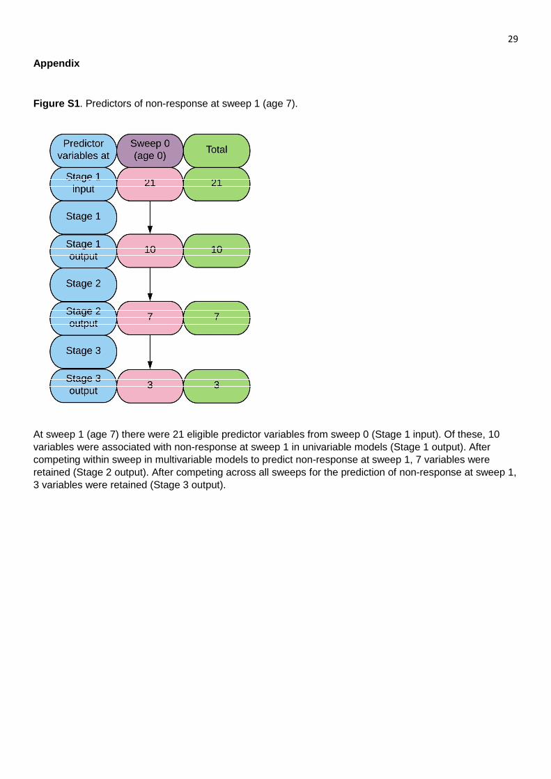
Figure S1. Predictors of non-response at sweep 1 (age 7).

At sweep 1 (age 7) there were 21 eligible predictor variables from sweep 0 (Stage 1 input). Of these, 10 variables were associated with non-response at sweep 1 in univariable models (Stage 1 output). After competing within sweep in multivariable models to predict non-response at sweep 1, 7 variables were retained (Stage 2 output). After competing across all sweeps for the prediction of non-response at sweep 1, 3 variables were retained (Stage 3 output).

30 Figure S2. Predictors of non-response at sweep 2 (age 11).

At sweep 2 (age 11) there were 71 eligible predictor variables across sweeps 0 to 1 (Stage 1 input). Of these, 27 variables were associated with non-response at sweep 2 in univariable models (Stage 1 output). After competing within sweep in multivariable models to predict non-response at sweep 2, 16 variables were retained (Stage 2 output). After competing across all sweeps for the prediction of non-response at sweep 2, 6 variables were retained (Stage 3 output).

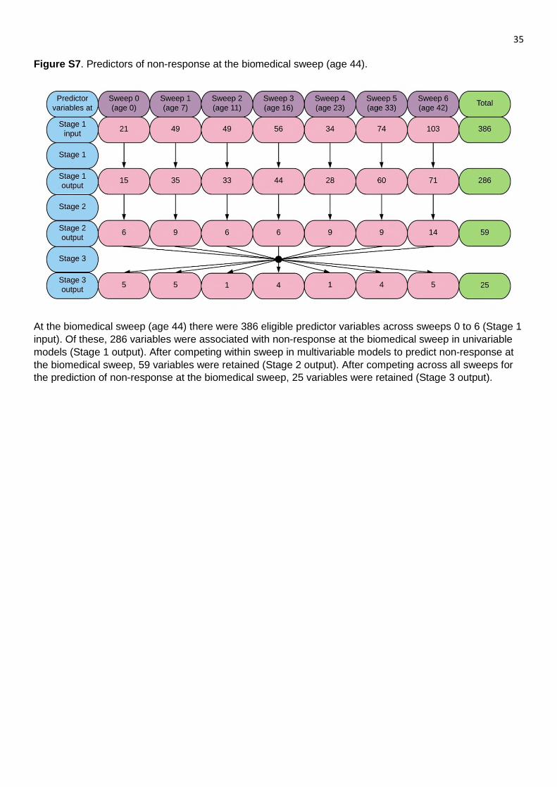
35 Figure S7. Predictors of non-response at the biomedical sweep (age 44).

At the biomedical sweep (age 44) there were 386 eligible predictor variables across sweeps 0 to 6 (Stage 1 input). Of these, 286 variables were associated with non-response at the biomedical sweep in univariable models (Stage 1 output). After competing within sweep in multivariable models to predict non-response at the biomedical sweep, 59 variables were retained (Stage 2 output). After competing across all sweeps for the prediction of non-response at the biomedical sweep, 25 variables were retained (Stage 3 output).


BM: Biomedical. At sweep 7 (age 46) there were 434 eligible predictor variables across sweeps 0 to the biomedical sweep (Stage 1 input). Of these, 321 variables were associated with non-response at sweep 7 in univariable models (Stage 1 output). After competing within sweep in multivariable models to predict non-response at sweep 7, 73 variables were retained (Stage 2 output). After competing across all sweeps for the prediction of non-response at sweep 7, 24 variables were retained (Stage 3 output).


BM: Biomedical. At sweep 8 (age 50) there were 498 eligible predictor variables across sweeps 0 to 7 (Stage 1 input). Of these, 358 variables were associated with non-response at sweep 8 in univariable models (Stage 1 output). After competing within sweep in multivariable models to predict non-response at sweep 8, 59 variables were retained (Stage 2 output). After competing across all sweeps for the prediction of non-response at sweep 8, 27 variables were retained (Stage 3 output).


BM: Biomedical. At sweep 9 (age 55) there were 587 eligible predictor variables across sweeps 0 to 8 (Stage 1 input). Of these, 478 variables were associated with non-response at sweep 9 in univariable models (Stage 1 output). After competing within sweep in multivariable models to predict non-response at sweep 9, 103 variables were retained (Stage 2 output). After competing across all sweeps for the prediction of non-response at sweep 9, 31 variables were retained (Stage 3 output).

39

Table S1. Age-specific mortality rates – NCDS vs ONS data

Age group NCDS observed

deaths Person-years Rate 95% CI ONS rate

0 403 79544 0.005066 0.004595 0.005586 0.005286

5-9 33 78958 0.000418 0.000297 0.000588 0.000423

10-14 29 78823 0.000368 0.000256 0.000529 0.000286

15-19 48 78638 0.00061 0.00046 0.00081 0.000586

20-24 50 78382 0.000638 0.000484 0.000842 0.000643

25-29 46 78158 0.000589 0.000441 0.000786 0.000581

30-34 43 77922 0.000552 0.000409 0.000744 0.000747

35-39 72 77671 0.000927 0.000736 0.001168 0.001043

40-44 118 77205 0.001528 0.001276 0.001831 0.001505

45-49 154 76562 0.002011 0.001718 0.002356 0.002214

50-55 218 75682 0.002881 0.002522 0.003289 0.003166

55-57 197 44825 0.004395 0.003822 0.005054 0.004147

Deaths from ONS; population estimates from the Human Mortality Database. We first compute the entry time (year of birth) and follow-up time (The earlier between time of death and end of observation period, set at 2015). Then, we split the follow-up time for each subject into current age intervals, and then for each interval sum the total follow-up time and outcomes across all subjects. We then estimate a rate for each interval. This was implemented in Stata through the following steps: To expand the records according to current age we specify date of birth as the entry as well as origin of the time scale: stset exit, fail(dead) enter(entry) origin(entry) id(NCDSID) . We then split each person’s total follow-up time into current age intervals. Each person will then have multiple records in the dataset (unless they enter and exit within the same age interval). A new variable ‘ageband’ is created to indicate the age band of the record. stsplit ageband, at (0,5(5)57). Finally, we calculate a rate for each age band: strate ageband, per(1000) // adding ‘per(1000)’ we were able to obtain accurate person-years (table S1 does not include PY per 1,000. All features (e.g. rate) are in “natural” scale.

40 Table S2. Estimated risk ratios and 95% confidence intervals for predictors of non-response at sweep 1 (age 7) (n = 17,262).

Sweep Variable RR 95% CI

Sweep 0 Region

(age 0) North 1.12 0.85, 1.49

Midlands 1.23 0.91, 1.68

East & South East 1.59 1.20, 2.12

South & South West 1.48 1.09, 2.02

Wales 1.00 (reference)

Scotland 1.35 0.99, 1.84

Number of persons per room [per person] 1.10 1.05, 1.16


I 1.00 (reference)

II 0.66 0.51, 0.84

III non-manual 0.65 0.49, 0.86

III manual 0.59 0.47, 0.73

IV 0.72 0.57, 0.92

V 0.80 0.62, 1.02

Results from sequential multiple imputation analyses in which potential predictors of non-response at a given sweep are adjusted for previously identified potential predictors of non-response at that sweep and previous sweeps (i.e. not at subsequent sweeps).



Sweep 0 Mother's present marital status

(age 0) Married/Twice married 1.00 (reference)

Unmarried/Stable union/Separated, divorced, widowed 1.65 1.35, 2.01

Sweep 1 Number of kids under 21 in the household, including living away [per kid] 0.91 0.87, 0.95

(age 7) Common difficulties age 7 (mother) [per difficulty] 0.90 0.86, 0.94

Hospital admissions [per admission] 0.91 0.86, 0.96

Cognitive ability summary [per unit] 0.85 0.80, 0.91

Non-response at sweep 1

Respondent 5.76 5.28, 6.28

Non-respondent 1.00 (reference)




Sweep 0 Region

(age 0) North 1.17 0.94, 1.45

Midlands 1.39 1.11, 1.73

East & South East 1.70 1.38, 2.10



Scotland 0.94 0.73, 1.20


(age 7) Mother worked birth to 5

No 1.20 1.08, 1.33

Yes 1.00 (reference)

Ever breastfed

Never breastfed 1.21 1.10, 1.35

Ever breastfed 1.00 (reference)

Sweep 2 Non-response at sweeps 1-2

(age 11) Complete response 1.00 (reference)

Incomplete response 2.84 2.62, 3.06




Sweep 0 Region

(age 0) North 1.24 1.06, 1.44

Midlands 1.19 1.02, 1.40

East & South East 1.45 1.25, 1.69



Scotland 1.14 0.96, 1.35


Sex of child

Male 1.18 1.12, 1.25

Female 1.00 (reference)


I 1.00 (reference)

II 1.01 0.85, 1.21


III manual 1.13 0.96, 1.32

IV 1.14 0.96, 1.36

V 1.46 1.23, 1.73

Sweep 1 Family moves since child's birth [per move] 1.10 1.08, 1.12

(age 7) Cognitive ability summary [per unit] 0.86 0.83, 0.89

Dad reads to child

Every week sometimes 1.00 (reference)

Hardly ever 1.13 1.06, 1.22

Sweep 2 Area of world in which mother born

(age 11) British islands 1.00 (reference)

Eire & Ulster 1.30 1.13, 1.50

Europe including USSR 1.02 0.83, 1.26

Outside Europe 1.49 1.29, 1.72

Number of family moves since child’s birth [per move] 1.09 1.05, 1.12

Cognitive ability summary [per 10 units] 0.91 0.88, 0.94

Number of household amenities [per unit] 0.91 0.88, 0.95

Sweep 3 Number of family moves since child’s birth [per move] 1.07 1.04, 1.11

(age 16) Sum of favourable learning environments/outcomes re sex educ etc) [per

10 units]

0.88 0.82, 0.94

Conduct problems [per unit] 1.10 1.07, 1.13

Non-response at sweeps 1-3

Complete response 1.00 (reference)





Sweep 0 Number of persons per room [per person] 1.11 1.09, 1.13

(age 0) Sex of child

Male 1.22 1.16, 1.28



I 1.00 (reference)

II 1.06 0.90, 1.24


III manual 1.21 1.04, 1.40

IV 1.30 1.11, 1.52

V 1.72 1.47, 2.00

Sweep 1 Family moves since child's birth [per move] 1.04 1.02, 1.06

(age 7) Social problems (alcoholism etc.) [per problem] 1.10 1.07, 1.13


Summary of medical conditions [per condition] 0.96 0.94, 0.98

Ever breastfed



Sweep 2 Child’s positive activities outside school [per 10 activities] 0.89 0.84, 0.94

(age 11) Cognitive ability summary [per 10 units] 0.89 0.87, 0.92

Number of household amenities per unit] 0.93 0.90, 0.97

Sweep 3 Number of family moves since child’s birth [per move] 1.06 1.03, 1.08

(age 16) How long since child drank alcohol

Less than 1 week 1.00 (reference)

2 to 4 weeks 0.97 0.88, 1.07

5+ weeks 1.04 0.95, 1.13

Do not remember 1.11 1.01, 1.22

Never had one 1.27 1.14, 1.41

Test 2 – mathematics comprehension [per 10 units] 0.82 0.76, 0.88

Sum of favourable learning environments/outcomes re sex educ etc) [per

10 units]

0.86 0.81, 0.91

Sweep 4 Type of current accommodation

(age 23) House 1.00 (reference)

Bungalow 0.92 0.76, 1.11

PB flat 1.23 1.14, 1.33

SC flat 1.13 1.00, 1.27

Other 1.11 0.94, 1.32


Didn’t vote 1.24 1.17, 1.32

Voted 1.00 (reference)

Economic status

Economically inactive 1.10 0.99, 1.21

Full-time education 1.12 0.92, 1.36

Employed 1.00 (reference)

Unemployed 1.20 1.10, 1.31

Number of voluntary activities (youth club, church etc.) 0.94 0.91, 0.97


45








Male 1.19 1.13, 1.25



I 1.00 (reference)

II 0.94 0.80, 1.11


III manual 1.18 1.02, 1.36

IV 1.22 1.05, 1.43

V 1.51 1.30, 1.77

Sweep 1 Cognitive ability summary [per unit] 0.83 0.80, 0.85

(age 7)

Sweep 2 Area of world in which father born

(age 11) British islands 1.00 (reference)

Eire & Ulster 1.14 0.99, 1.31

Europe including USSR 1.12 0.94, 1.34

Outside Europe 1.33 1.17, 1.50

Child’s positive activities outside school [per 10 activities] 0.89 0.85, 0.94


Sweep 3 How long since child drank alcohol

(age 16) Less than 1 week 1.00 (reference)

2 to 4 weeks 1.05 0.96, 1.14

5+ weeks 1.08 1.00, 1.18


Never had one 1.27 1.13, 1.42

Sum of good activities performed outside school [per activity] 0.97 0.96, 0.98


Sweep 4 Legal marital status

(age 23) Single 1.05 0.97, 1.13

Married 1.00 (reference)

Separated/divorced/widowed 1.32 1.16, 1.51


Didn’t vote 1.25 1.18, 1.33


Sweep 5 Type of accommodation

(age 33) Detached house, etc. 1.00 (reference)

Semi house/bungalow 0.99 0.87, 1.12

Terraced house 1.01 0.88, 1.14

Flat/maisonette/Converted flat, rooms, caravan, miscellaneous 1.26 1.11, 1.44

Current member of a Trade Union/Staff Association

None of those 1.15 1.06, 1.25

Yes-Trade Union 1.00 (reference)

Social capital score (people turn to for advice, support) [per 10 units] 0.81 0.77, 0.85

Life contentment score [per unit] 0.95 0.93, 0.98



47



48 Table S8. Estimated risk ratios and 95% confidence intervals for predictors of non-response at biomedical sweep (age 44) (n = 16,003).



(age 0) Abnormality during pregnancy

No 1.00 (reference)

Yes 1.07 1.03, 1.11

Social class of mother's father when she left school

I & II 1.00 (reference)


III manual 1.07 1.01, 1.14

IV 1.02 0.95, 1.11

V 1.12 1.04, 1.21

Sex of child

Male 1.07 1.03, 1.11



I 1.00 (reference)

II 1.08 0.95, 1.23


III manual 1.25 1.12, 1.40

IV 1.32 1.16, 1.49

V 1.55 1.38, 1.75

Sweep 1 Dad stayed on at school after minimum age

(age 7) No 1.12 1.06, 1.20


Attendance

Good attendance 1.00 (reference)

Frequent short absences 1.17 1.09, 1.26

Long absences 1.10 1.02, 1.19

Social problems (alcoholism etc.) [per problem] 1.04 1.02, 1.06


Body mass index [per kg/m2] 1.02 1.01, 1.04

Sweep 2 Cognitive ability summary [per 10 units] 0.90 0.88, 0.92

(age 11)

Sweep 3 Emotional or behavioural problem

(age 16) No abnormality 1.00 (reference)

Any condition or handicap 1.23 1.14, 1.32



2 to 4 weeks 1.05 0.99, 1.12

5+ weeks 1.06 1.00, 1.14


Never had one 1.21 1.11, 1.31



Sweep 4 Voted in 1979 general election

(age 23) Didn’t vote 1.13 1.08, 1.19


Sweep 5 Any work related training course since March 1981

49

(age 33) No 1.12 1.05, 1.19


Number of hospital admissions since March 1981 [per admission] 0.95 0.93, 0.98

Driven/ridden after drinking alcohol in last 7 days

Doesn’t drive 1.14 1.07, 1.21

Yes 0.88 0.80, 0.96

No 1.00 (reference)


Sweep 6 Normally has access to a car or van

(age 42) Yes 1.00 (reference)

No 1.12 1.04, 1.20

Doesn’t drive 1.13 1.05, 1.22


No 1.18 1.11, 1.25



No 1.00 (reference)

Yes 1.15 1.11, 1.21

Has a computer at home

No 1.09 1.04, 1.14










Male 1.14 1.10, 1.19



I 1.00 (reference)

II 1.09 0.96, 1.25


III manual 1.27 1.13, 1.43

IV 1.34 1.18, 1.52

V 1.62 1.43, 1.83


(age 7) No 1.13 1.06, 1.20


Attendance

Good attendance 1.00 (reference)

Frequent short absences 1.16 1.07, 1.25

Long absences 1.09 1.01, 1.18



Sweep 2 Source of family income last year

(age 11) Other sources 1.17 1.09, 1.26

Employment 1.00 (reference)

Child’s positive activities outside school [per 10 activities] 0.93 0.89, 0.97


Sweep 3 Local Authority & voluntary schools

(age 16) Comprehensive 1.05 1.00, 1.11

Grammar 1.10 0.99, 1.22

Secondary modern 1.00 (reference)

Other 1.23 1.11, 1.37

Wish could leave school at 15 – study child

Yes 1.15 1.09, 1.22

No 1.00 (reference)

Uncertain 1.00 0.93, 1.08



2 to 4 weeks 1.06 0.99, 1.13

5+ weeks 1.09 1.02, 1.17


Never had one 1.26 1.17, 1.37


Sweep 4 Number of accidents since 16th birthday [per accident] 1.03 1.01, 1.04

(age 23) Voted in 1979 general election

Didn’t vote 1.16 1.11, 1.22



(age 33) Didn’t vote 1.12 1.06, 1.19

51



Sweep 6 Participated in NCDS V

(age 42) No 1.33 1.24, 1.43



No 1.00 (reference)

Yes 1.19 1.12, 1.26


No 1.14 1.06, 1.23


BM sweep Current legal marital status

(age 44) Single, never married 1.04 0.92, 1.17

Married, first and only 1.00 (reference)

Remarried 1.13 1.02, 1.24


Is current accommodation owned or rented?

Other 1.22 1.11, 1.35

Owner 1.00 (reference)

Non-response at sweeps 1-biomedical



Results from sequential multiple imputation analyses in which potential predictors of non-response at a given sweep are adjusted for previously identified potential predictors of non-response at that sweep and previous sweeps (i.e. not at subsequent sweeps). BM: Biomedical.





Male 1.11 1.07, 1.46



I 1.00 (reference)

II 0.98 0.86, 1.12


III manual 1.18 1.05, 1.32

IV 1.27 1.12, 1.43

V 1.45 1.28, 1.63

Sweep 1 Social problems (alcoholism etc.) [per problem] 1.07 1.04, 1.09

(age 7) Cognitive ability summary [per unit] 0.84 0.82, 0.86

Summary of medical conditions [per one condition] 0.97 0.96, 0.98


(age 11) Conduct problems [per unit] 1.04 1.02, 1.06

Sweep 3 Child's school attendance [per 10 units] 0.97 0.96, 0.98

(age 16) How long since child drank alcohol


2 to 4 weeks 1.04 0.97, 1.11

5+ weeks 1.02 0.95, 1.10


Never had one 1.21 1.10, 1.32




(age 23) Single 1.04 0.99, 1.10




Didn’t vote 1.18 1.13, 1.24


Economic status

Economically inactive 1.10 1.02, 1.17

Full-time education 1.14 0.95, 1.37

Employed 1.00 (reference)

Unemployed 1.16 1.08, 1.24


(age 33) Didn’t vote 1.16 1.10, 1.23



Life contentment score [per unit] 0.96 0.95, 0.98

Sweep 6 Frequency of eating biscuits and cakes of all kinds [per category of

decreasing consumption]

1.04 1.03, 1.06

(age 42) Is current accommodation owned or rented?

Other 1.19 1.10, 1.28

Owner 1.00 (reference)

53


No 1.28 1.18, 1.39


Ever wanted improve your maths?

No 1.13 1.06, 1.21



No 1.14 1.06, 1.22


BM

sweep

Consent to access NHS records

(age 44) Consent not given 1.54 1.35, 1.75

Consent given 1.00 (reference)

How many children do you have living with you aged 18 or less [per child] 0.91 0.86, 0.95

How many natural (biological) children have you ever had [per child] 1.08 1.04, 1.13

Sweep 7 Non-response at sweeps 1-7

(age 46) Complete response 1.00 (reference)





Sweep 0 Mother’s age [per 10 years] 0.93 0.89, 0.97

(age 0) Number of persons per room [per person] 1.06 1.04, 1.08

Parity [per child] 1.04 1.02, 1.05

Social class of mother's father when she left school



III manual 1.08 1.01, 1.15

IV 1.08 1.00, 1.17

V 1.17 1.09, 1.27

Sex of child

Male 1.13 1.09, 1.18





III manual 1.35 1.26, 1.43

IV 1.41 1.31, 1.53

V 1.69 1.57, 1.82


(age 7) No 1.15 1.07, 1.23




Ever breastfed




(age 11) Conduct problems [per unit] 1.03 1.02, 1.05

Sweep 3 Child receiving help at school – backwardness

(age 16) No 1.00 (reference)

Yes 1.13 1.06, 1.20

Child's school attendance [per 10 units] 0.97 0.96, 0.98



2 to 4 weeks 1.03 0.96, 1.10

5+ weeks 1.04 0.97, 1.11


Never had one 1.22 1.13, 1.31




(age 23) Single 1.12 1.03, 1.21




Didn’t vote 1.16 1.11, 1.21


55

Sweep 5 Telephone in home

(age 33) No 1.12 1.05, 1.19


How much physical effort in job [per category] 1.05 1.02, 1.07


Didn’t vote 1.16 1.11, 1.21


Housing tenure

Other 1.14 1.08, 1.21

Owners 1.00 (reference)


Sweep 6 Participated in NCDS V

(age 42) No 1.35 1.25, 1.45



No 1.14 1.06, 1.23


BM sweep Self-rated general health [per category of decreasing health] 1.12 1.06, 1.18

(age 44)

Sweep 7 Marital status - de facto

(age 46) Married 1.00 (reference)

Cohabiting (living as a couple) 0.99 0.89, 1.11

Single (and never married) 1.18 1.07, 1.32

Separated, divorced or widowed 1.23 1.12, 1.35

Sweep 8 Total number of natural children [per child] 1.05 1.03, 1.08

(age 50) Employer provided pension scheme

No 1.13 1.06, 1.20






56 Table S12. Results from sensitivity analysis using LASSO at Stage 2.

Stage 1 variables

Stage 2 variables Predictors Non-response Log-binomial LASSO

Sweep 0 (age 0) Sweep 1 (age 7) 10 7 9 Sweep 2 (age 11) 5 4 5 Sweep 3 (age 16) 10 4 9 Sweep 4 (age 23) 16 4 13 Sweep 5 (age 33) 15 5 9 Sweep 6 (age 42) 14 4 11 Biomedical sweep (age 44) 15 6 10 Sweep 7 (age 46) 16 6 12 Sweep 8 (age 50) 13 8 11 Sweep 9 (age 55) 16 7 13 Sweep 1 (age 7) Sweep 2 (age 11) 22 12 20 Sweep 3 (age 16) 14 9 12 Sweep 4 (age 23) 34 8 10 Sweep 5 (age 33) 35 11 27 Sweep 6 (age 42) 34 4 14 Biomedical sweep (age 44) 35 9 25 Sweep 7 (age 46) 37 10 22 Sweep 8 (age 50) 35 7 22 Sweep 9 (age 55) 38 8 28

57 Table S13. Estimated risk ratios and 95% confidence intervals for predictors of non-response at sweep 1

(age 7) (n = 17,262) after LASSO variable selection at Stage 2


Sweep 0 Region

(age 0) North 1.11 0.84, 1.48

Midlands 1.24 0.92, 1.68

East & South East 1.59 1.20, 2.10



Scotland 1.34 0.99, 1.82


Abnormality during pregnancy

No 1.00 (reference)

Yes 2.23 2.05, 2.43


I 1.00 (reference)

II 0.61 0.48, 0.78


III manual 0.58 0.47, 0.72

IV 0.73 0.58, 0.93

V 0.78 0.62, 1.00


58 Table S14. Estimated risk ratios and 95% confidence intervals for predictors of non-response at sweep 2

(age 11) (n = 17,017) ) after LASSO variable selection at Stage 2.


Sweep 0 Mother's present marital status

(age 0) Married/Twice married 1.00 (reference)

Unmarried/Stable union/Separated, divorced, widowed 1.64 1.33, 2.01

Abnormality during pregnancy

No 1.00 (reference)

Yes 1.47 1.34, 1.62


(age 7) Common difficulties age 7 (mother) [per difficulty] 0.92 0.88, 0.95


Non-response at sweep 1

Respondent 5.49 5.02, 6.00

Non-respondent 1.00 (reference)


59

Table S15. Estimated unadjusted risk ratios and 95% confidence intervals for consistent predictors (selected in at least 50% of possible sweeps) of non-response at sweeps 1-5 (ages 7-33).

Sweep 1 (age 7)

Sweep 2 (age 11)

Sweep 3 (age 16)

Sweep 4 (age 23)

Sweep 5 (age 33)


Non-response at previous sweep(s)

Complete response NA NA 1.00 (reference) 1.00 (reference) 1.00 (reference) 1.00 (reference)

Incomplete response NA NA 6.11 5.62, 6.65 3.02 2.80, 3.26 2.30 2.18, 2.42 2.64 2.51, 2.77

Sweep 0 (age 0)


1.09 1.04, 1.15 NS NS NS NS 1.13 1.10, 1.16 1.14 1.12, 1.17

Sex of child

Male NS NS NS NS NS NS 1.18 1.12, 1.25 1.22 1.17, 1.28

Female NS NS NS NS NS NS 1.00 (reference) 1.00 (reference)


I 1.00 (reference) NS NS NS NS 1.00 (reference) 1.00 (reference)

II 0.66 0.51, 0.84 NS NS NS NS 1.01 0.85, 1.21 1.06 0.90, 1.24

III non-manual 0.65 0.49, 0.84 NS NS NS NS 0.91 0.75, 1.10 1.06 0.89, 1.25

III manual 0.59 0.47, 0.73 NS NS NS NS 1.13 0.96, 1.33 1.21 1.04, 1.40

IV 0.72 0.57, 0.92 NS NS NS NS 1.14 0.95, 1.36 1.30 1.11, 1.52

V 0.80 0.62, 1.02 NS NS NS NS 1.47 1.24, 1.74 1.72 1.48, 2.01

Sweep 1 (age 7)

Cognitive ability summary [per unit] NA NA 0.85 0.79, 0.91 NS NS 0.81 0.79, 0.84 0.79 0.77, 0.81


NA NA NS NS NS NS NS NS 1.13 1.11, 1.16

Sweep 2 (age 11)

Cognitive ability summary [per 10 units]

NA NA NA NA NS NS 0.87 0.86, 0.89 0.85 0.84, 0.86

Sweep 3 (age 16)

Conduct problems [per unit] NA NA NA NA NA NA 1.20 1.17, 1.23 NS NS

60


Less than 1 week NA NA NA NA NA NA NS NS 1.00 (reference)

2 to 4 weeks NA NA NA NA NA NA NS NS 0.99 0.90, 1.09

5+ weeks NA NA NA NA NA NA NS NS 1.12 1.03, 1.22

Do not remember NA NA NA NA NA NA NS NS 1.21 1.10, 1.33

Never had one NA NA NA NA NA NA NS NS 1.60 1.45, 1.77


NA NA NA NA NA NA NS NS 0.70 0.67, 0.73

Sweep 4 (age 23)


Didn’t vote NA NA NA NA NA NA NA NA 1.47 1.38, 1.56

Voted NA NA NA NA NA NA NA NA 1.00 (reference)


Single NA NA NA NA NA NA NA NA NS NS

Married NA NA NA NA NA NA NA NA NS NS

Separated/divorced/widowed NA NA NA NA NA NA NA NA NS NS

NA : Not applicable (predictor variable observed concurrently with or subsequent to non-response variable); NS: Not selected.

61

Table S16. Estimated unadjusted risk ratios and 95% confidence intervals for consistent predictors (selected in at least 50% of possible sweeps) of non-response at sweeps 6-9 (ages 42-55).

Sweep 6 (age 42)

Biomedical sweep

(age 44)

Sweep 7 (age 46)

Sweep 8 (age 50)

Sweep 9 (age 55)


Non-response at previous sweeps

Complete response 1.00 (reference) 1.00 (reference) 1.00 (reference) 1.00 (reference) 1.00 (reference)

Incomplete response 4.50 4.21, 4.81 4.08 3.85, 4.31 8.32 7.59, 9.11 7.32 6.67, 8.04 7.49 6.81, 8.23

Sweep 0 (age 0)


1.14 1.11, 1.16 1.11 1.09, 1.13 1.12 1.10, 1.13 1.11 1.09, 1.13 1.13 1.11, 1.14

Sex of child

Male 1.19 1.14, 1.25 1.07 1.03, 1.11 1.15 1.10, 1.19 1.11 1.07, 1.16 1.13 1.09, 1.18

Female 1.00 (reference) 1.00 (reference) 1.00 (reference) 1.00 (reference) 1.00 (reference)


I 1.00 (reference) 1.00 (reference) 1.00 (reference) 1.00 (reference) 1.00 (reference)

II 0.94 0.80, 1.11 1.08 0.95, 1.23 1.09 0.96, 1.24 0.98 0.86, 1.12 1.00 (reference)

III non-manual 1.02 0.86, 1.20 1.14 1.00, 1.30 1.14 0.99, 1.24 1.06 0.92, 1.21 1.11 1.01, 1.22

III manual 1.18 1.02, 1.36 1.25 1.12, 1.40 1.27 1.13, 1.43 1.18 1.05, 1.32 1.35 1.26, 1.43

IV 1.22 1.04, 1.43 1.32 1.16, 1.49 1.34 1.18, 1.52 1.26 1.12, 1.63 1.42 1.31, 1.53

V 1.52 1.30, 1.77 1.55 1.38, 1.75 1.62 1.43, 1.83 1.45 1.28, 1.64 1.70 1.58, 1.83

Sweep 1 (age 7)

Cognitive ability summary [per unit] 0.78 0.76, 0.81 0.80 0.79, 0.82 0.78 0.76, 0.80 0.80 0.78, 0.82 0.75 0.74, 0.77


NS NS 1.10 1.09, 1.12 1.11 1.10, 1.13 1.10 1.08, 1.12 1.12 1.10, 1.13

Sweep 2 (age 11)

Cognitive ability summary [per 10 units] 0.84 0.83, 0.85 0.86 0.85, 0.87 0.85 0.84, 0.86 0.86 0.85, 0.87 0.83 0.82, 0.84

Sweep 3 (age 16)

Conduct problems [per unit] 1.19 1.67, 1.22 1.16 1.14, 1.18 NS NS 1.17 1.14, 1.19 1.19 1.17, 1.21

62


Less than 1 week 1.00 (reference) 1.00 (reference) 1.00 (reference) 1.00 (reference) 1.00 (reference)

2 to 4 weeks 1.06 0.97, 1.16 1.07 1.01, 1.14 1.07 1.00, 1.14 1.04 0.97, 1.12 1.04 0.97, 1.12

5+ weeks 1.15 1.06, 1.25 1.12 1.05, 1.20 1.17 1.09, 1.25 1.06 0.98, 1.14 1.10 1.03, 1.17

Do not remember 1.20 1.09, 1.32 1.20 1.12, 1.29 1.22 1.14, 1.31 1.17 1.09, 1.25 1.20 1.12, 1.28

Never had one 1.57 1.42, 1.74 1.42 1.31, 1.53 1.50 1.39, 1.61 1.42 1.30, 1.54 1.46 1.36, 1.56


NS NS 0.72 0.70, 0.74 0.70 0.68, 0.72 0.71 0.69, 0.74 0.65 0.63, 0.67

Sweep 4 (age 23)


Didn’t vote 1.45 1.37, 1.54 1.28 1.22, 1.33 1.32 1.27, 1.38 1.34 1.28, 1.41 1.35 1.29, 1.41

Voted 1.00 (reference) 1.00 (reference) 1.00 (reference) 1.00 (reference) 1.00 (reference)


Single 1.06 1.00, 1.13 NS NS NS NS 0.98 0.93, 1.03 1.01 0.96, 1.05

Married 1.00 (reference) NS NS NS NS 1.00 (reference) 1.00 (reference)

Separated/divorced/widowed 1.50 1.43, 1.69 NS NS NS NS 1.32 1.19, 1.46 1.38 1.26, 1.50

Sweep 5 (age 33)


Didn’t vote NS NS NS NS 1.40 1.32, 1.47 1.43 1.36, 1.51 1.46 1.40, 1.52

Voted NS NS NS NS 1.00 (reference) 1.00 (reference) 1.00 (reference)

Social capital score (people turn to for advice, support) [per 10 units]

0.65 0.62, 0.69 0.71 0.69, 0.73 0.72 0.70, 0.74 0.73 0.71, 0.75 0.71 0.68, 0.73

Sweep 6 (age 42)


No NA NA 2.20 2.09, 2.31 1.73 1.64, 1.83 1.70 1.61, 1.80 1.77 1.69, 1.87

Yes NA NA 1.00 (reference) 1.00 (reference) 1.00 (reference) 1.00 (reference)


No NA NA 1.00 (reference) 1.00 (reference) NS NS NS NS

Yes NA NA 1.32 1.25, 1.39 1.31 1.23, 1.39 NS NS NS NS

63


No NA NA NS NS 1.48 1.38, 1.58 1.45 1.35, 1.54 1.55 1.45, 1.66

Yes NA NA NS NS 1.00 (reference) 1.00 (reference) 1.00 (reference)

BM sweep (age 44)

Sweep 7 (age 46)

Marital status - de facto

Married NA NA NA NA NA NA NS NS 1.00 (reference)

Cohabiting (living as a couple) NA NA NA NA NA NA NS NS 1.16 1.03, 1.31

Single (and never married) NA NA NA NA NA NA NS NS 1.48 1.34, 1.63

Separated, divorced or widowed NA NA NA NA NA NA NS NS 1.52 1.40, 1.65

Sweep 8 (age 50)

Total number of natural children [per child]

NA NA NA NA NA NA NA NA 1.06 1.04, 1.09

Employer provided pension scheme

No NA NA NA NA NA NA NA NA 1.58 1.47, 1.69

Yes NA NA NA NA NA NA NA NA 1.00 (reference)

NA : Not applicable (predictor variable observed concurrently with or subsequent to non-response variable); NS: Not selected; BM: Biomedical. Note that no biomedical sweep variables were selected as consistent predictors of non-response.

64

Derivation of consistent predictors of non-response

Cognitive ability at 7: Principal Component Analysis (PCA) score. PCA indicators were the

Problem Arithmetic Test score, Total score on Copying Designs Test, Drawing a Man Test score and the Southgate Group Reading Test score.

Cognitive ability at 11: A general ability test score consisting of 40 verbal and 40 non-verbal

items (range 0 to 80). Children were tested individually by teachers, who recorded the answers for the tests. For the verbal items, children were presented with an example set of four words that were linked either logically, semantically, or phonologically. For the non-verbal tasks, shapes or symbols were used. The children were then given another set of three words or shapes or symbols with a blank. Participants were required to select the missing item from a list of five alternatives.

Conduct problems at 11 and 16: Conduct problems and affective symptoms in childhood

and adolescence were assessed using the modified version of the Rutter ‘A’ scale [1]. This version of the scale was completed by the mothers of the participants at ages 7 and 11 years, and from both mother and teachers at age 16. Mother and teacher reports were employed to capture symptoms both at home and school, as is well known that maternal and teacher reports are weakly correlated and that triangulating information from multiple informants may bring unique insights into children’s behaviour and may predict poor child and adolescent outcomes in ways that the individual informants' reports do not [2]. Conduct problems refer to behaviour such as being disobedient, destructive, being irritable and being involved in fights. A latent summary score of four conduct problems derived from a 2 parameter was included in the analysis. We derived latent summary of conduct problems at 16 by modelling the probability of response to the Rutter items with a 2 parameter probit latent variable measurement model [3, 4] and calculated a latent trait summary score.

Social participation at age 23: Sum of voluntary activities.

Social Capital at age 33: Number of people you turn to for support.

Social participation at age 42: Ever being a member of an organisation (political party, environmental charity, voluntary group, women groups, parents/school/tenant organisations).

Social participation at age 50: Sum score of membership in various organisations: Political

party, Trade Union, Environmental group, Parents, School association, Residents Group, neighbourhood watch, Religious Group or Church Organisation, Voluntary Service group, Other Community, civic group, Social, Working men's club, Sports club, Professional organisation, Scouts, Guides organisation, Other Organisation.

References

1. Rutter, M., J. Tizard, and K. Whitmore, Education, health and behaviour. 1970: Longman Publishing Group.

2. De Los Reyes, A., Introduction to the special section: More than measurement error: Discovering meaning behind informant discrepancies in clinical assessments of children and adolescents. J Clin Child Adolesc Psychol, 2011. 40(1): p. 1-9.

65

3. Muthén, B., A general structural equation model with dichotomous, ordered categorical, and continuous latent variable indicators. Psychometrika, 1984. 49(1): p. 115-132.

4. Rabe-Hesketh, S. and A. Skrondal, Classical latent variable models for medical research. Statistical Methods in Medical Research, 2008. 17(1): p. 5-32.

66

Restoring sample representativeness

In order to investigate whether the identified at Stage 3 predictors of non-response have the potential to restore sample representativeness in NCDS despite attrition, we compared estimates from NCDS participants at age 50 with the known population distribution of educational attainment and marital status derived from the Office for National Statistics Annual Population Survey in 2008. Within this analysis we compared the relative effectiveness of the identified predictors of non-response compared to variables associated with education and marital status. We also investigated whether the original distributions of paternal social class at birth and cognitive ability at age 7 can be replicated using NCDS data from age 55.

67

Figure S11. Percentage of those without educational qualifications at age 50 in the Annual Population Survey and NCDS before and after adjustment for missing data.

APS GB: Annual Population Survey = Born in Great Britain in 1958 (derived by the Office for National Statistics) APS All: Annual Population Survey - Born in Great Britain or elsewhere in 1958 (derived by the Office for National Statistics) NCDS50: Estimate using observed educational attainment at age 50. NCDS50 MI: Estimate after multiple imputation using predictors of educational attainment at age 50 (see below) and predictors of non-response at age 50 (see Table S10) as auxiliary variables. Predictors of educational attainment at age 50: Maternal interest in cohort member’s education at age 7; Overcrowding at age 11; Being off school > 1 month at age 11; Family financial difficulties at age 11; Housing tenure at age 7; Mother reading to CM at age 7; Maternal smoking during pregnancy; Maternal employment (birth to 5 years); Training courses by age 23; Child’s positive activities at school age 11; Parity at birth; Nocturnal enuresis at 7; Ever breastfed; Smoking.

10

12

14

16

18

Pe

rcen

tage

witho

ut e

du

catio

na

l qu

alif

ica

tion

s

APS GB(N = 3993)

APS All(N = 4596)

NCDS50(N = 9783)

NCDS50 MI(N = 15,806)

68

Figure S12. Percentage of those single and never married by age 50 in the Annual Population Survey and NCDS before and after adjustment for missing data.

APS GB: Annual Population Survey = Born in Great Britain in 1958 (derived by the Office for National Statistics) APS All: Annual Population Survey - Born in Great Britain or elsewhere in 1958 (derived by the Office for National Statistics) NCDS50: Estimate using observed marital status at age 50. NCDS50 MI: Estimate after multiple imputation using predictors of marital status at age 50 (see below) and predictors of non-response at age 5 (see Table S10) as auxiliary variables. Predictors of marital status at age 50: Marital status at ages 23, 33, 42, 4 and 46.

10

11

12

13

14

Pe

rcen

tage

sin

gle

& n

ever

marr

ied

APS GB(N = 3993)

APS All(N = 4596)

NCDS50(N = 9789)

NCDS50 MI(N = 15,806)

69

Figure S13. Social class of mother’s husband at birth before and after adjustment for missing data.

Imputation phase of MI included all predictors of response at age 55 (see Table S11) and social class at birth only for cohort members that participated at age 55.

44

.55

5.5

6P

erc

en

tag

e in

pro

fessio

na

l so

cia

l cla

ss

70

Figure S14. Cognitive ability at age 7 before and after adjustment for missing data.

Imputation phase of MI included all predictors of response at age 55 (see Table S11) and cognitive ability at age 7 only for cohort members that participated at age 55.

-.0

50

.05

.1.1

5M

ea

n c

og

niti

ve a

bili

ty a

t a

ge

7

improving the plausibility of the missing at random

Documents