Improving the Measurement of Socially Unacceptable Attitudes and Behaviors With Item Response Theory MARIA ORLANDO, LISA H. JAYCOX, DANIEL F. MCCAFFREY, GRANT N. MARSHALL

WR-383

April 2006

WORK ING P A P E R

This product is part of the RAND Health working paper series. RAND working papers are intended to share researchers’ latest findings and to solicit informal peer review. They have been approved for circulation by RAND Health but have not been formally edited or peer reviewed. Unless otherwise indicated, working papers can be quoted and cited without permission of the author, provided the source is clearly referred to as a working paper. RAND’s publications do not necessarily reflect the opinions of its research clients and sponsors.

is a registered trademark.

1

Improving the Measurement of Socially Unacceptable Attitudes and Behaviors With Item

Response Theory

Maria Orlando, Lisa H. Jaycox, Daniel F. McCaffrey, Grant N. Marshall

RAND Health

*RAND Corporation, Santa Monica CA

†National Cancer Institute

2

Abstract

Assessment of socially unacceptable behaviors and attitudes via self-report is likely to

yield skewed data that may be vulnerable to measurement non-invariance. Item response

theory (IRT) can help address these measurement challenges. This paper illustrates

application of IRT to data from a teen dating violence intervention study. Three factors

reflecting teens’ attitudes about dating violence were identified, and items from these 3

scales were subjected to IRT calibration and evaluated for differential item functioning

(DIF) by gender. The IRT scores displayed superior measurement properties relative to

the observed scale scores, and in 1 of the 3 factors, inferences about group mean

differences were impacted by the presence of DIF. This application demonstrates how

IRT analysis can improve measurement of socially unacceptable behaviors and attitudes.

3

Researchers have devoted considerable attention to the development of prevention

and early intervention programs aimed at changing the manner in which youths think

about and relate to themselves and others. Generally speaking, these programs strive to

reduce the incidence of deviant behavior such as substance use, dating-related youth

violence, and bullying. Although evidence suggests that some of these programs may be

having the desired impact (e.g., Ellickson, McCaffrey, Ghosh-Dastidar & Longshore,

2003; Foshee et al., 2004; Frey et al., 2005; Wolfe et al., 2003), careful assessment of

these interventions can be hampered by two measurement challenges that have not been

fully recognized or addressed by the field. In our view, continued progression of

knowledge in the adolescent prevention field can benefit from wider understanding and

appreciation of the value of modern measurement theory and methods in addressing these

challenges.

Accurate assessment of intervention effects that target socially unacceptable

behaviors and attitudes is difficult primarily because respondents are unlikely to report

engaging in socially unacceptable behaviors or to endorse attitudes that condone these

behaviors. As a result, items and scales developed to measure these constructs typically

yield highly skewed response distributions, especially in samples from the general

population that are typical of prevention studies. The skew in these responses makes the

assumption of continuity untenable, requiring that raw responses be collapsed to two or

three response categories and modeled as binomial or multinomial outcomes. Not only

does this practice obscure variability that may be of interest, it also limits the types of

analyses that can be performed.

4

An additional challenge is that these measures may fail to display measurement

invariance (Reise, Widaman, & Pugh, 1993) according to important demographic

subgroups of interest. At the item level, non-invariance indicates non-equivalent

measurement properties for individuals who have the same overall level of the measured

construct, but are from different subgroups. For example, items assessing attitudes about

dating violence may be particularly vulnerable to non-equivalence according to gender.

Teens of both genders may have similar levels of acceptance of dating violence, but be

differentially accepting of items that portray particular types of violence, or represent the

male as victim rather than perpetrator. The potential non-equivalence across groups can

confound interpretation of observed group differences. To avoid this possible confound,

non-equivalence should be evaluated and taken into account in modeling.

Addressing skewed response distributions and potential measurement non-

invariance is difficult with classical test theory approaches, but can be handled to some

degree with item response theory (IRT; Hambleton & Swaminathan, 1985). No analytic

technique can change a distribution that is mostly zeros into one that is normal, but IRT

can help. First, IRT scoring converts categorical responses into an interval scale allowing

for analysis of continuous outcomes. Second, this non-linear conversion helps alleviate

the impact of highly skewed data by accentuating differences between 0 and 1 and

attenuating differences between single intervals higher up on the scale. Thus, IRT allows

one to assign different weight to responses depending on where they are on the scale.

Furthermore, IRT is well-suited to evaluation of item and scale invariance through

assessment of differential item functioning (DIF; Holland & Wainer, 1993), and provides

5

a useful framework for modeling DIF to yield IRT scores that take the identified DIF into

account.

This paper illustrates the application of IRT to data collected as part of an ongoing

intervention study of dating violence among teens (Jaycox et al., under review). Youth

dating violence is a problem of paramount importance. Various studies indicate that

roughly 20% of all youths have been in abusive dating relationships (Aizenman &

Kelley, 1988; Arias, Samios, & O'Leary, 1987; Bergman, 1992). Focusing solely on past

year prevalence estimates in high school students, approximately 10% of girls and 9% of

boys report exposure to dating violence (Grunbaum et al., 2002). An emerging body of

evidence suggests that exposure to youth dating violence may have pernicious

consequences, leading to increased substance abuse, unhealthy weight control, poorer

health, sexual risk behavior, pregnancy and suicidality among victims (Silverman et al.,

2001; Waigandt et al., 1990).

In the intervention study providing data for this application, scales reflecting

attitudes about dating violence were planned as the main outcome measures. The scales

consisted of multiple items with polytomous Likert-type response options, and the

intention was to treat them as continuous measures for analytic purposes. However,

routine treatment of these data proved unsatisfactory because of the two measurement

challenges discussed above: the response distributions of these items were highly skewed,

and the item content made measurement invariance across gender highly suspect (i.e.,

items addressed opposite-sex dating violence with each gender as perpetrator and victim).

For example, the meaning of an item such as “It is okay for a girl to hit a boy if the he hit

her first” may be somewhat different for a female versus a male respondent, since the

6

respondent may identify more with the person of the same gender. Therefore, in an effort

to optimize the precision of the outcome measures, after determining the factor structure

of the item set, we used IRT to evaluate item and scale invariance with respect to gender.

As part of this process, we also examined the properties of various scoring metrics (i.e.,

raw scores, IRT scores that ignore gender DIF, IRT scores that account for gender DIF)

to identify the best metric for future analyses. Before describing this application, we first

provide a brief overview of IRT and describe the characteristics of IRT that are

particularly useful in this context.

Item response theory

IRT comprises a collection of modeling techniques that offer many advantages

over classical test theory. By considering the correlations among the item responses, IRT

extracts more information from the data than does classical test theory. Thus, more

information can be gained about the relationship between the items on the test and the

construct being measured (Embretson, 1996; Hambleton & Swaminathan, 1985;Lord,

1980). An IRT model specifies the relationship between an individual’s observed

responses to a set of items and the unobserved (or latent) trait that is being measured by

the item set. One result of an IRT calibration is a set of continuous trace lines, most

commonly defined as logistic functions, which describe the probability of endorsing each

response category of an item given the scale value of the latent construct being measured.

For items with dichotomous responses, the two-parameter logistic (2PL) model is

often applied. This model yields a trace line that is described by the location (b) and slope

(a) parameters. The b parameter is the point along the trace line at which the probability

of a positive response for a dichotomous item is 50%. The larger the location parameter,

7

the more of the measured construct a respondent must have to endorse that item. The a

parameter represents the slope of the trace line at the value of the location parameter and

indicates the extent to which the item is related to the underlying construct. A steeper

slope indicates a closer relationship to the construct.

A generalization of the 2PL model that permits estimation of multiple difficulty

parameters associated with ordinal responses is Samejima’s graded response model

(Samejima, 1969, 1997). Let denote an individual’s underlying value on the latent

construct of interest. A general statement of Samejima’s graded model, for ordered

responses x = k, k = 0, 1, 2, …, m, is:

1

1 1( ) *( ) *( 1)1 exp 1 expi ik i ik

T x k T k T ka b a b

,

in which ai is the slope parameter, bik is the item location parameter, and T*(k) is the trace

line for the probability that a response is in category k or higher, for each value of

IRT-Scores. In IRT, the relationship between the item responses and the latent

trait (as represented by the item trace lines) is used to convert item responses into a scaled

estimate of . The trait estimate is on an interval scale that is usually arbitrarily defined

with a mean of 0 and a standard deviation of 1, resulting in a score distribution that is

similar to the z-score distribution (Suen, 1990). Estimating a score using IRT methods

involves the multiplication of all the trace lines corresponding to a person’s responses to

each question. For example, on a three-item test, a response of “no” to the first two items

and “yes” to the third item would result in three trace lines. A posterior distribution is

formed by multiplying the three trace lines together with a prior distribution (that is

usually normal) for the unknown latent construct , and the IRT-score is calculated as the

8

average of this posterior distribution (Thissen & Wainer, 2001). One of the unique

features of IRT is that the reliability of the score estimate is variable, and depends on

where the score lies along the underlying continuum (Hambleton & Swaminathan, 1985;

Suen, 1990), thus IRT scores for individuals have associated standard errors of

measurement that reflect the uncertainty of the estimated score.

IRT and Differential Item Functioning. An IRT model is ideally suited to defining

differential item functioning (DIF), which can refer to situations in which items behave

differently for various subgroups after controlling for the overall differences between

subgroups on the construct being measured (Holland & Wainer, 1993; Thissen,

Steinberg, & Wainer, 1988). For example, if the statement “It is okay for a girl to hit a

boy if the he hit her first” contains gender DIF, the item trace lines will be different

according to gender, either in the sense that the probabilities of endorsement are

uniformly unequal for the two groups (the b parameters are different), or that the item is

more discriminating for one group than the other (the a parameters are different). In

either case, the presence of DIF implies the need for different item parameters according

to group membership, and different item parameters yield different trace lines, resulting

in different scores. Thus, a scale containing an item with DIF according to gender, for

example, would yield non-identical IRT-scores for males and females whose response

patterns were exactly the same, provided that the DIF was identified and accounted for in

the scoring algorithm.

The fact that DIF is characterized by the need for unique item parameters

according to group membership means that DIF can be specifically modeled, and can also

be detected by testing the statistical significance of differences between item parameters

9

for the two groups. There are a number of ways to construct such statistical tests. One

approach that is applied in this paper uses model-based likelihood ratio comparison tests

to evaluate the significance of observed differences in parameter estimates between

groups (Thissen, Steinberg, & Wainer, 1993; Wainer, Sireci, & Thissen, 1991).

The model comparison approach has several advantages: it can be performed

using available software (e.g., MULTILOG, Thissen, 1991; IRTLRDIF, Thissen, 2001), the

definition of DIF is intuitive and clear (a statistically significant difference between item

parameter estimates for the two groups), and the likelihood-based model comparison test

is a common statistical test with known distributional properties. It also has been

suggested that DIF analyses employing model-based likelihood ratio tests are more

powerful than are other DIF detection approaches (Teresi, Kleinman, & Ocepek-

Welikson, 2000; Thissen et al., 1993; Wainer, 1995).

To construct the nested model comparisons, the groups first must be linked so that

the items for both groups can be calibrated simultaneously. The linking serves as a basis

for which to estimate the group mean difference. The best way to link the groups is to

identify a subset of items, referred to as “anchor items,” that are judged a priori to be

unbiased, and to use these as a basis with which to link the groups (Embretson, 1996).

Recent research on the likelihood-based model comparison approach to DIF detection

indicates that a single-item anchor is often sufficient to reliably estimate the group mean

difference (i.e., link the two groups), although an anchor set of 3 or more items is

preferable (Wang & Yeh, 2003). If there is no a priori set of anchor items, they can be

identified in an iterative fashion. The iterations serve to “purify” the linkage, which is

first accomplished based on all the items in the scale (except the item being tested), and

10

finally based on only those items judged to be DIF-free. This purification process is

common to many linking and equating procedures (e.g.Baker, Al-Karni, & Al-Dosary,

1991; Candell & Drasgow, 1988; Raju, van der Linden, & Fleer, 1995).

Once a set of anchor items has been established, each of the studied items can be

tested for DIF relative to the now-specified anchor. For each studied item, all of the

item’s parameters can be first tested as a group by comparing the fit of a model that

estimates separate item parameters for the two groups to the fit of a model that constrains

these estimates to be equal for the two groups. If this model comparison test indicates that

at least one of the study item’s parameters might differ between groups (e.g., at a nominal

= .05), parameter-specific model comparison tests can be constructed and evaluated in

a similar fashion so that the source of the DIF can be identified.

In this study, we used modern measurement theory to first identify the factor

structure of a group of items reflecting adolescents’ acceptance of various forms of cross-

gender aggression. Next, we refined our measurement of the identified factors using IRT,

testing each of the items for DIF according to gender, and evaluating the impact of the

identified DIF on inferences about group differences. The method and results are

described below, and implications for measurement of this particular construct, as well as

extreme attitudes in general are discussed.

Application

Data and Sample

Participants. Data are from a study evaluating a dating violence prevention

curriculum. This evaluation employed an experimental design with random assignment

11

by cluster of 9th grade Health classes in Los Angeles United School District (LAUSD).

Eligible high schools were those serving majority Latino populations. Clusters were

assigned to an immediate or delayed intervention (control group) and both groups were

followed for 6-months. This study uses responses from the first survey administration,

(i.e., the baseline survey prior to any student receiving the intervention), for a sample of

N=2575.1 The sample was nearly evenly split according to gender with 1263 males and

1312 females. The majority (91%) of the participants were Latino, with an average age of

14.5 years (SD= 1.04).

Measure. Analyses examine 14 items reflecting adolescents’ attitudes about

aggression in dating situations. Eight of the items were drawn from the Prescribed Norms

scale (Foshee et al., 1996), and ask respondents to indicate on a 4-point scale (1=Strongly

Agree to 4=Strongly Disagree) their extent of agreement with statements about dating

violence (e.g., “Girls sometimes deserve to be hit by the boys they date”, “It is ok for a

girl to hit a boy if he hit her first”). These 8 items were reverse-scored for analyses so

that for all items, a higher score indicated more acceptance of violence. Six additional

items were between-gender items from an approval of retaliation scale (NOBAGS;

Huesmann & Guerra, 1997). These items ask participants to indicate on a 4-point scale

(1=Really Wrong to 4=Perfectly OK) the extent to which the response to the situation

was acceptable (e.g., “Suppose a girl says something bad to a boy, do you think it’s

wrong for the boy to scream at her?”). Abbreviated content for all 14 items is listed in

Table 1.

1 The analyses reported in Jaycox et al. (2005) use a sample of 2540 students because those analyses excludes blocks of schools (including both those randomized to intervention or control condition) where at least one school failed to provide data or complete the program as assigned. The responses from all students provide information on the measurement model and are included in the current application.

12

Analytic Approach

Assessing Dimensionality. After examining the descriptive statistics for all items,

exploratory factor analyses (EFA) were conducted on the 14 items to determine their

factor structure and create appropriate scales for further analysis. All items were assumed

to be categorical for these analyses, which were conducted in Mplus (Muthen & Muthen,

1998-2004) using the unweighted least squares estimator. EFA solutions were examined

for the entire sample as well as separately for boys and girls. Several criteria were used to

determine the optimal number of factors, including the number of eigenvalues>1, the

scree plot of the eigenvalues, the interpretability of candidate solutions, and the extent of

correspondence across male and female respondents.

IRT DIF Evaluation and Scoring. Factors identified in the EFA were examined

separately using Samejima’s graded IRT model. First, the scales were evaluated for

gender DIF using the likelihood ratio approach implemented with the freeware program

IRTLRDIF (Thissen, 2001). The parameter-specific DIF significance evaluations were

adjusted for multiple tests using the Benjamini-Hochberg adjustment (Benjamini &

Hochberg, 1995) and an overall alpha level of .01. Although these criteria for

significance are rather stringent, it is appropriate to control for multiple tests in the

absence of any a priori hypotheses (i.e., when all items are being tested for DIF).

Additionally, the model comparison approach to DIF detection is fairly powerful (Teresi

et al., 2000; Wainer, 1995), and we were interested in accepting DIF only when there was

strong evidence for its presence.

On the basis of the DIF analyses, we specified a version of Samejima’s graded

IRT model that allowed item parameters with DIF to vary by gender for each scale. The

13

model parameters were estimated and IRT scale scores generated using MULTILOG

(Thissen, 1991), which generates item parameter estimates and standard errors, together

with other summary statistics, including item information, reliability estimates, and the

focal group overall mean and standard deviation (relative to a N(0,1) distribution for the

reference group). In this application, the boys served as the reference group, and the girls

comprised the focal group.

Model checking. Although there are currently no formal absolute tests for IRT

model fit, there are some methods for examining the appropriateness of the model. We

performed two distinct checks to determine whether the model was an adequate refection

of the data. First, we visually examined the concordance between the observed and model

predicted category responses for each item using bar charts. Strong concordance in these

charts would imply that the model is able to re-create the data. Second, we examined

non-parametric models of the item responses using TESTGRAPH (Ramsay, 1993) to

evaluate whether the functional form imposed by the parametric IRT model was

reasonable. In this examination, similarity between the shape of the category response

functions from the parametric and non-parametric analyses would lend support for the

IRT model.

Evaluating scores. The impact of allowing for DIF between genders on the

models and scores was evaluated in several ways. First, plots of category, item, and scale

response functions were generated to provide a visual representation of the effect size of

the DIF. Next, to examine the impact of the DIF more closely at the factor-score level,

IRT-scores were generated for each factor from models that specified the DIF and models

that ignored the DIF. Correlations between the DIF-adjusted and non-DIF-adjusted IRT

14

scores, as well as between each of these IRT scores and observed scale scores were

calculated for each factor, and the corresponding scatterplots were examined to determine

the impact of the IRT calibrations on the score distributions. In these plots, a lack of

correspondence between the IRT scores and the scale scores would imply that the IRT

scoring approach impacts the score distribution (presumably in an advantageous way),

and a lack of correspondence between the IRT DIF-adjusted and IRT non-DIF-adjusted

scores would indicate that the DIF “matters” and should be incorporated into the scoring

model. Finally, t-tests comparing males and females on each of these three types of

scores were generated for each of the factors to determine whether the scoring had an

impact on the estimated group mean differences. Specifically, if the inferences about

group differences varied according to the type of score used, the use of IRT-scores (either

DIF-adjusted or non-DIF-adjusted) for modeling these factors as outcomes would be

supported.

Results

Assessing Dimensionality. The exploratory factor analysis generated 4

eigenvalues>1. Solutions for up to 4 factors were examined, and the 3-factor solution was

adopted for this set of items. The 3-factor solution yielded distinct item loadings, and

provided a better fit to the data than the 2-factor solution. Additionally, all three factors

were clearly interpretable, and the solution was similar across genders. In this solution,

displayed for the full sample in Table 1, 5 of the 8 Prescribed Norms items (PN) loaded

only on the first factor (PN1-PN4, PN6; Cronbach’s alpha=.88). These items all involve

boys hitting their girlfriends under minimal provocation. The distributions of responses to

15

these items were highly skewed and they had very little variance – almost all respondents

chose the “strongly disagree” or “somewhat disagree” options for these items. The

second factor consists of 3 items from the NOBAGS scale (NB) and two from Prescribed

Norms scale: NB3, NB4, NB5, PN5, and PN8 (Cronbach’s alpha=.71). These are all

items about girls’ aggression on boys after some provocation. Item PN5 loaded

significantly on both the first and second factors, but because of the content, it was

included in the second factor. The third factor has 4 items: NB1, NB2, NB6, and PN7

(Cronbach’s alpha=.55). These items are all about boys’ aggression on girls after some

provocation. Item PN7 loaded significantly on both the first and third factors, but because

of the content, it was included in the third factor. Although the internal consistency for

this factor was low, we felt that the factor analysis results and the commonality of the

items’ content strongly indicated that there was a distinct construct to be measured. In

addition, even with low reliability the factor would be adequate for use as an outcome for

purposes of evaluating an intervention, although the low reliability would limit the power

for detecting program effects.

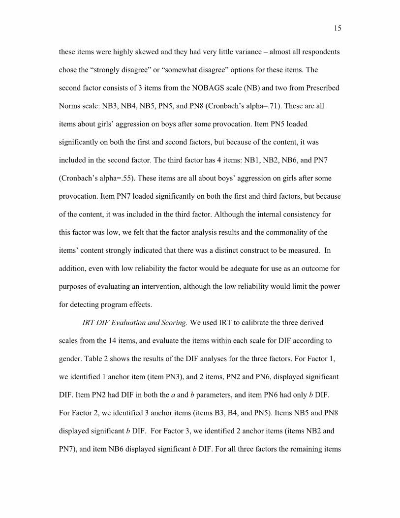
IRT DIF Evaluation and Scoring. We used IRT to calibrate the three derived

scales from the 14 items, and evaluate the items within each scale for DIF according to

gender. Table 2 shows the results of the DIF analyses for the three factors. For Factor 1,

we identified 1 anchor item (item PN3), and 2 items, PN2 and PN6, displayed significant

DIF. Item PN2 had DIF in both the a and b parameters, and item PN6 had only b DIF.

For Factor 2, we identified 3 anchor items (items B3, B4, and PN5). Items NB5 and PN8

displayed significant b DIF. For Factor 3, we identified 2 anchor items (items NB2 and

PN7), and item NB6 displayed significant b DIF. For all three factors the remaining items

16

not explicitly mentioned here showed potential DIF in our initial screening and did not

meet the criteria for being anchor items. However, in the final analyses with the chosen

anchor items, these items did not have significant DIF according to the stringent criteria

used in this application.

The next step was to estimate the parameters of the chosen model for each factor

using MULTILOG. The item parameter estimates and their standard errors from these final

calibrations are reported in Table 3. The items for all three factors tended to be fairly

discriminating with all but one slope estimate exceeding 1.2. In this context, a slope of 1

corresponds to a factor loading of about .5, and a slope of 2 to a factor loading of about

.76 (McLeod, Swygert, & Thissen, 2001; Takane & de Leeuw, 1987). The magnitude of

the item slopes for Factor 1 are somewhat misleading, however, as they are most likely

artificially inflated due to the high degree of covariance relative to variance in these

items. The b-parameter values indicate that higher response categories corresponding to

items in Factor 1 tend to be endorsed only at high levels of acceptance of violence (e.g.,

all b3 values for Factor 1 are higher than 2), whereas items in the other two factors,

particularly Factor 2, represent a broader segment of the underlying continuum they are

measuring. The location parameters for each factor are all estimated relative to a mean of

0 for the boys. Overall, the girls had lower acceptance of violence than boys on all three

factors with means of -.45, -.10, and -.20 for Factors 1-3 respectively.

Assessment of fit strongly supported the use of the IRT models for the items of

Factors 2 and 3, whereas the strong inter-item correlation for Factor 1 might be

inconsistent with the assumptions of the IRT model causing some lack of fit. For all

three factors, the model-predicted category responses for each item corresponded very

17

closely with the observed frequencies, lending support for the models. The non-

parametric item response functions were also reasonably similar to their model based

counterparts, with the exception of items in Factor 1; the category response functions for

items in this factor were steeper and more distinct in the parametric models than in the

non-parametric analysis. This is most likely due to the high degree of covariance among

the item responses (65% of respondents answered 1 to every item on factor 1), which is

utilized directly by the parametric model but not by the non-parametric model. In light of

the lack of correspondence in item trace lines across the two analyses, the parametric IRT

model and corresponding scores for Factor 1 should be interpreted cautiously.

Figure 1 shows the category (top panel) and item (bottom panel) response

functions for girls and boys for item NB5 from Factor 2 (“Suppose a boy hit a girl, do

you think its OK for the girl to hit him back?”). As shown in Table 3, the three location

parameters for this item are all lower for boys than for girls. Thus, the DIF in this item

indicates that controlling for the overall acceptance of girl-on-boy violence, boys are

slightly more accepting than girls of this particular act, being less likely to say it is “really

wrong” and more likely to say it is “perfectly OK.” This results in boys having a higher

expected score on this item than girls with the same level of overall acceptance of girl-

on-boy violence.

Item PN6 from Factor 1 and item PN8 in Factor 2 also show this pattern of DIF

(see parameter values in Table 3). The DIF in item PN2, Factor 1 is more difficult to

interpret because of the difference in the slope parameters. Essentially, this item (“A girl

who makes her boyfriend jealous on purpose deserves to be hit.”) is more strongly related

to the underlying construct of acceptance of violence for girls than for boys. Finally, the

18

observed DIF in item NB6 from Factor 3 (“If a girls hits a boy, do you think its OK for

the boy to hit her back?”) indicates that controlling for the overall acceptance of violence,

girls are slightly more accepting than boys of this particular act, being less likely to say it

is “really wrong” and more likely to say it is “perfectly OK.”

Figure 2 displays girls’ and boys’ expected total scores for each factor as a

function of overall acceptance of violence. This relationship is generated based on the

IRT model that specifies separate item parameters for the DIF items (i.e., the parameters

in Table 3), so the expected total scores differ for boys and girls (if the model did not

account for DIF, the two lines would be completely coincident). In general for Factor 1

(top panel), the DIF does not have a great deal of impact at the factor level (the expected

total score lines for girls and boys are nearly coincident across the continuum), but boys

do have slightly higher expected total scores for this factor than girls with the same

overall level of acceptance of violence, especially at levels of acceptance of violence

between 0 and 1. Modeling the DIF in Factor 2 also results in higher expected total scores

for boys than girls. The effect is perhaps less pronounced than in Factor 1, but is more

constant across the continuum of acceptance of violence. The effect of DIF on the

expected total score for Factor 3 is in the opposite direction. For this factor, modeling the

DIF results in higher expected total scores for girls than boys. The effect is slight, but

discernable between acceptance of violence values of 0 and 2.

A final set of descriptive analyses was conducted to inform the decision regarding

the most appropriate type of scores to use in future analyses, the observed scale scores,

the DIF-adjusted IRT scores, or IRT scores that ignore the DIF. Scatterplots of the scale

scores and DIF-adjusted IRT scores, such as that shown in Figure 3 (for Factor 3)

19

provided a visual representation of how the IRT rescaling affects the score distribution.

(The scale scores range from 5-20 for Factors 1 & 2, and 4-16 for Factor 3). In general,

the IRT scores give more weight when moving up one scale score point at the very

bottom of the scale than when moving up one point somewhere else on the scale,

implying that according to the IRT model, endorsing violence to any extent is a bigger

step than endorsing it a little more than others who have endorsed it. At the high end of

the scale, the change in one scale score point is less important.

The shape of the scatterplots confirmed that the IRT scores would be useful, but

did not clarify whether it was necessary to adjust for the small amount of observed DIF in

the factors. To inform this decision, the estimated group mean differences between girls

and boys were examined on each of the factors using the three different types of scores.

This information, listed in Table 4, indicates that regardless of score type, boys have

higher means than girls (more accepting of violence) for all 3 factors. For Factors 1 and

2, the results are the same regardless of type of score. However, the significance of the

group differences varies for Factor 3 depending on which type of score is used. For

Factor 3, the difference between girls and boys is only significant using the DIF-adjusted

scores. Thus adjusting for the DIF has an impact on inferences about group means for 1

of the 3 factors. Based on this information, we made the decision to use DIF-adjusted

scores in future analyses of these data so that observed gender differences could be

confidently interpreted as true differences, not confounded by a lack of measurement

invariance.

Discussion

20

Measurement of socially unacceptable behaviors and attitudes poses difficult

challenges not easily met by classical test theory methods. Although many individuals do

not endorse item responses reflecting agreement with extreme attitudes, real variability in

attitudes about behaviors such as dating violence does exist. Accurate assessment of

these constructs is essential to inform decisions of policymakers and prevention and

intervention specialists on how best to influence change.

IRT methods offer some potential advantages over methods derived from classical

test theory. IRT can convert categorical responses to an interval scale and can help

alleviate the impact of skewed response distributions. In addition, IRT provides a useful

framework for the evaluation of measurement invariance through DIF analyses. In the

IRT framework, any significant lack of measurement invariance that is identified can

easily be examined and accounted for in both the parameter estimates and resultant

scores. The most obvious source of non-invariance in studies of cross-gender aggression

would be according to gender.

In the application presented here, we found some items that were invariant and

could act as anchor items, and other items that appear to be interpreted somewhat

differently by boys and girls. Given the fact that societal norms are more lenient about

female-on-male violence than male-on-female violence (e.g., Price & Byers, 1999), it is

not surprising that boys and girls might respond to some items differently based on

looking at the problem from differing perspectives. However, such differences can be

very troublesome in studies that include both genders. Basic gender differences,

differential program impact on boys and girls, and interactions with gender could be

misleading if the items are behaving differently based on gender. Thus, IRT’s capacity to

21

account for DIF can increase precision in measurement, and lead to a greater ability to

evaluate hypotheses.

As this application demonstrates, IRT analysis can help address the measurement

challenges associated with assessment of socially unacceptable behaviors and attitudes.

However, an important lesson learned is that the measures currently in existence to assess

attitudes related to dating violence (and other related constructs) are not optimal. Further

research to improve the assessment of socially unacceptable behaviors should consider

non-standard approaches to item generation. For example, in order to understand the

nuances in teen attitudes towards cross-gender aggression, our research team has begun

work that allows teens to articulate their thoughts about dating violence scenarios as they

unfold. Preliminary examination of the data collected to date shows us that (a) a variety

of factors influence teens’ perceptions of dating violence (e.g., whether the perpetrator is

male or female, a friend or a stranger, gender of respondent), and (b) that teens express

approval and disapproval of dating violence in a number of ways. The insights provided

by this exercise can be translated into more appropriate and discriminating items that

teens will respond to with greater variability.

In addition to considering novel approaches such as this, future assessment

development should include evaluation of measurement invariance during instrument

construction. Whether the developer wants to exclude variant items or include them and

adjust for them in the scoring, this practice will provide important information and will

minimize biased inferences about group differences in the construct being measured.

22

References

Aizenman, M., & Kelley, G. (1988). The incidence of violence and acquaintance rape in

dating relationships among college men and women. Journal of College Student

Development, 29(4), 305-311.

Arias, I., Samios, M., & O'Leary, K. D. (1987). Prevalence and correlates of physical

aggression during courtship. Journal of Interpersonal Violence, 2(1), 82-90.

Baker, F. B., Al-Karni, A., & Al-Dosary, I. M. (1991). EQUATE: A computer program

for the test characteristic method of IRT equating. Applied Psychological

Measurement, 15, 78.

Benjamini, Y., & Hochberg, Y. (1995). Controlling the false discovery rate: a practical

and powerful approach to multiple testing. Journal of the royal statistical society,

Series B(57), 289-300.Bergman, L. (1992). Dating violence among high school

students. Social Work, 37(1), 21-27.

Candell, G. L., & Drasgow, F. (1988). An iterative procedure for linking metrics and

assessing item bias in item response theory. Applied Psychological Measurement,

12(3), 253-260.

Ellickson, P.L., McCaffrey, D., Ghosh-Dastidar, B. & Longshore, D.L. (2003). New

inroads in preventing adolescent drug use: Results from a large-scale trial of

Project ALERT in middle schools. American Journal of Public Health, 93(11),

1830-1836.

Embretson, S. E. (1996). The new rules of measurement. Psychological Assessment, 8,

341-349.

23

Foshee, V. A., Bauman, K. E., Ennett, S. T., Linder, G. F., Benefield, T., & Suchindran,

C. (2004). Assessing the Long-Term Effects of the Safe Dates Program and a

Booster in Preventing and Reducing Adolescent Dating Violence Victimization

and Perpetration. American Journal of Public Health, 94(4), 619-624.

Foshee, V. A., Linder, G. F., Bauman, K. E., Langwick, S. A., Arriaga, X. B., Heath, J.

L., McMahon, P. M., & Bangdiwala, S. (1996). The Safe Dates Project:

theoretical basis, evaluation design, and selected baseline findings. American

Journal of Preventive Medicine, 12(5 Suppl), 39-47.

Frey, K. S., Hirschstein, M. K., Snell, J. L., Edstrom, L. V. S., MacKenzie, E. P., &

Broderick, C. J. (2005). Reducing Playground Bullying and Supporting Beliefs:

An Experimental Trial of the Steps to Respect Program. Developmental

Psychology, 41(3), 479-491.

Grunbaum, J. A., Kann, L., Kinchen, S. A., Williams, B., Ross, J. G., Lowry, R., &

Kolbe, L. (2002). Youth Risk Behavior Surveillance - United States, 2001.

Surveillance Summaries. 51(No. SS-4), 1-21.

Hambleton, R. K., & Swaminathan, H. (1985). Item response theory: principles and

applications.Boston, MA: Kluwer-Nijhoff.

Holland, P. W., & Wainer, H. (1993). Differential Item Functioning. Hillsdale, NJ:

Lawrence Erlbaum Associates.

Huesmann, L. R., & Guerra, N. G. (1997). Children's normative beliefs about aggression

and aggressive behavior. Journal of Personality and Social Psychology, 72(2),

408-419.

24

Jaycox, L.H., McCaffrey, D.F., Eiseman, E., Aronoff, J. Shelley, G.A., Collins, R.L., &

Marshall, G.N. (Under review). Impact of a School-Based Dating Violence

Prevention Program among Latino Teens: A Randomized Controlled

Effectiveness Trial.

Lord, F. M. (1980). Applications of item response theory to practical testing problems.

Hillsdale, NJ: Earlbaum.

McLeod, L. D., Swygert, K. A., & Thissen, D. (2001). Factor analysis for items scored in

two categories. In D. Thissen & H. Wainer (Eds.), Test Scoring.Mahwah, New

Jersey: Lawrence Earlbaum & Associates.

Muthen, L. K., & Muthen, B. O. (1998-2004). Mplus Users Guide: The comprehensive

modeling program for applied researchers (3.0 ed.). Los Angeles: Muthen &

Muthen.

Price, E. L., & Byers, E. S. (1999). The Attitudes Towards Dating Violence Scales:

Development and initial validation. Journal of Family Violence, 14(4), 351-375.

Raju, N. S., van der Linden, W. J., & Fleer, P. F. (1995). IRT-Based Internal Measures of

Differential Functioning of Items and Tests. Applied Psychological Measurement,

19(4), 353-368.

Ramsay, J. O. (1993). TESTGRAF - A program for the graphical analysis of multiple

choice tst and questionnaire data (pp. 1-139). User's Manual.

Reise, S. P., Widaman, K. F., & Pugh, R. H. (1993). Confirmatory factor analysis and

item response theory: two approaches for exploring measurement invariance.

Psychological Bulletin, 114(3), 552-566.

25

Samejima, F. (1969). Estimation of latent ability using a response pattern of graded

scores. Unpublished manuscript.

Samejima, F. (1997). Graded response model. In W. J. v. d. L. a. R. K. Hambleton (Ed.),

Handbook of modern item response theory (pp. 85-100). New York: Springer-

Verlag.

Silverman, J. G., Raj, A., Mucci, L. A., & Hathaway, J. E. (2001). Dating violence

against adolescent girls and associated substance use, unhealthy weight control,

sexual risk behavior, pregnancy, and suicidality. The Journal of the American

Medical Association, 286(5), 572-579.

Suen, H., K. (1990). Principles of test theories.Hillsdale, NJ: Lawrence Earlbaum

Associates.

Takane, Y., & de Leeuw, J. (1987). On the relationship between item response theory and

factor analysis of discretized variables. Psychometrika, 52(3), 393-408.

Teresi, J. A., Kleinman, M., & Ocepek-Welikson, K. (2000). Modern psychometric

methods for detection of differential item functioning: application to cognitive

assessment measures. Statistics in Medicine, 19(11-12), 1651-1683.

Thissen, D. (1991). Multilog User's Guide: Multiples, Categorical Item Analysis and Test

Scoring Using Item Response Theory. Chicago, IL: Scientific Software.

Thissen, D. (2001). IRTLRDIF v.2.0b: Software for the computation of the statistics

involved in item response theory likelihood-ratio tests for differential item

functioning:LL Thurstone Psychometric Laboratory, University of North Carolina

at Chapel Hill.

26

Thissen, D., Steinberg, L., & Wainer, H. (1988). Use of Item Response Theory in the

Study of Group Differences in Trace Lines. In H. Wainer & H. Braun (Eds.), Test

Validity (pp. 147-169). Hillsdale, NJ: Lawrence Erlbaum.

Thissen, D., Steinberg, L., & Wainer, H. (1993). Detection of Differential Item

Functioning Using the Parameters of Item Response Models. In P. W. Holland &

H. W. (Eds.) (Eds.), Differential Item Functioning (pp. 67-114). Hillsdale, NJ:

Lawrence Erlbaum Associates.

Thissen, D., & Wainer, H. (Eds.). (2001). Test Scoring. Mahwah NJ: Lawrence Erlbaum

Associates.

Waigandt, A., Wallace, D. L., Phelps, L., & Miller, D. A. (1990). The impact of sexual

assault on physical health status. Journal of Traumatic Stress, 3(1), 93-102

Wainer, H. (1995). Precision and differential item functioning on a testlet-based test: The

1991 Law School Admissions Test as an example. Applied Measurement in

Education, 8(2), 157-186.

Wainer, H., Sireci, S. G., & Thissen, D. (1991). Differential Testlet Functioning:

Definitions and Detection. Journal of Educational Measurement, 28(3), 197-219.

Wang, W.-C., & Yeh, Y.-L. (2003). Effects of anchor item methods on differential item

functioning detection with the likelihood ratio test. Applied Psychological

Measurement., 27, 479-498.

Wolfe, D. A., Wekerle, C., Scott, K., Straatman, A.-L., Grasley, C., & Reitzel-Jaffe, D.

(2003). Dating violence prevention with at-risk youth: A controlled outcome

evaluation. Journal of Consulting & Clinical Psychology, 71(2), 279-291.

27

Table 1. Reference structure correlations from 3-factor EFA solution.

Factor 1 Factor 2 Factor 3

PN1. Girls sometimes deserve to be hit by boys they date. 0.88

PN2. Girl who makes boyfriend jealous on purpose deserves to be hit. 0.85

PN3. OK for boy to hit girlfriend if she did something to make him mad. 0.93

PN4. OK for boy to hit girlfriend if she insulted him in front of friends. 0.89

PN6. Sometimes boys have to hit girlfriends to get them under control. 0.80

PN5. Boys sometimes deserve to be hit by girls they date. 0.49 0.57

NB3. Boy says something bad to girl, OK for her to scream at him? 0.70

NB4. Boy says something bad to girl, OK for her to hit him? 0.86

NB5. Boy hits girl, OK for her to hit him back? 0.53

PN8. It is OK for a girl to hit a boy if he hit her first. 0.54

PN7. It is OK for a boy to hit a girl if she hit him first. 0.64 0.39

NB1. Girl says something bad to boy, OK for him to scream at her? 0.57

NB2. Girl says something bad to boy, OK for him to hit her? 0.54

NB6. Girl hits boy, OK for him to hit her back? 0.73Note: only coefficients .30 are included in this table. Items PN5 and PN7 had loadings

.30 on two factors. Their loadings on factor 1 (italicized entries) were ignored.

28

Table 2. Results of DIF analyses for three factors.

Test for item DIF (3 df) Test for a DIF (1 df) Test for b DIF (2 df)

Factor 1 (PN3 is anchor item)

Item -2LL p -2LL p -2LL p

PN4 3.6 .463

PN1 8.4 .078

PN5 17.5 .001* 4.3 .038 13.2 .004*

PN2 28.9 <.0001* 8.9 .003* 20.0 .0002*

Factor 2 (NB3, NB4, PN5 are anchor items)

Item -2LL p -2LL p -2LL p

PN8 17.9 .001* 3.5 .061 14.4 .002*

NB5 18.5 .001* 3.9 .048 14.5 .002*

Factor 3 (NB2, PN7 are anchor items)

Item -2LL p -2LL p -2LL p

NB1 11.1 .025

NB4 19.6 .001* 0.5 .48 19.1 .0003* Note: Asterisks indicate test was statistically significant at p<.01 after controlling for multiple tests with the NBenjamini-Hochburg adjustment. –2LL is the –2*loglikelihood value for the nested model comparison and is distributed as 2 with the specified df.

29

Table 3. Final item parameter estimates and their standard errors for the three factors.

a b1 b2 b3Factor 1

PN1 2.73 (0.16) 1.08 (0.04) 1.71 (0.07) 2.36 (0.12)

PN3 4.60 (0.31) 1.11 (0.03) 1.72 (0.06) 2.11 (0.09)

PN4 3.79 (0.23) 0.96 (0.03) 1.78 (0.06) 2.16 (0.09)

PN2 – girls 3.47 (0.30) 0.79 (0.05) 1.50 (0.10) 2.14 (0.20)

PN2 – boys 2.75 (0.19) 0.67 (0.04) 1.57 (0.08) 2.26 (0.13)

PN6 – girls 2.38 (0.10) 1.02 (0.06) 1.66 (0.10) 2.46 (0.20)

PN6 – boys 2.38 (0.10) 0.95 (0.05) 1.64 (0.07) 2.36 (0.12)

Factor 2

NB3 1.27 (0.06) -1.55 (0.08) 0.53 (0.05) 2.22 (0.11)

NB4 1.91 (0.09) 0.47 (0.04) 1.61 (0.07) 2.62 (0.12)

PN5 1.10 (0.05) 0.36 (0.06) 1.72 (0.11) 3.30 (0.20)

NB5 – girls 1.57 (0.05) -0.96 (0.06) -0.20 (0.06) 0.76 (0.06)

NB5 – boys 1.57 (0.05) -0.98 (0.07) -0.34 (0.06) 0.62 (0.06)

PN8 – girls 1.72 (0.06) -0.28 (0.05) 0.68 (0.06) 1.51 (0.08)

PN8 – boys 1.72 (0.06) -0.25 (0.05) 0.55 (0.06) 1.34 (0.07)

Factor 3

NB1 0.86 (0.06) -0.95 (0.09) 2.06 (0.15) 4.64 (0.34)

NB2 1.66 (0.18) 2.53 (0.18) 3.31 (0.28) 3.55 (0.32)

PN7 1.58 (0.09) 0.96 (0.06) 2.16 (0.11) 2.95 (0.17)

NB6 – girls 2.54 (0.10) 0.55 (0.04) 1.40 (0.06) 2.22 (0.12)

NB6 – boys 2.54 (0.10) 0.90 (0.05) 1.72 (0.07) 2.41 (0.12)

30

Table 4. Boys’ and girls’ factor means (SD) for 3 different types of scores.

Boys (N=1265) Girls (N=1310) Difference T-value (prob t)

Factor 1

Raw Score 6.474 (2.688) 5.706 (1.996) 0.768 (2.359) 8.15 (<.0001)

Non-DIF IRT -0.038 (0.811) -0.325 (0.649) 0.287 (0.733) 9.89 (<.0001)

DIF IRT -0.008 (0.802) -0.245 (0.637) 0.236 (0.723) 8.26 (<.0001)

Factor 2

Raw Score 10.190 (3.255) 9.761 (3.230) 0.429 (3.242) 3.32 (.0009)

Non-DIF IRT -0.015 (0.825) -0.108 (0.827) -0.093 (0.826) -2.84 (.0045)

DIF IRT -0.004 (0.817) 0.070 (0.834) -0.065 (0.825) -2.01 (.0449)

Factor 3

Raw Score 5.629 (1.728) 5.526 (1.561) 0.103 (1.645) 1.56 (.1185)

Non-DIF IRT 0.090 (0.708) 0.075 (0.694) 0.016 (0.701) 0.56 (.5721)

DIF IRT 0.010 (0.740) -0.094 (0.691) 0.104 (0.716) 3.69 (.0002)

31

NB5 girls (solid) and boys (dotted)

0.00

0.10

0.20

0.30

0.40

0.50

0.60

0.70

0.80

0.90

1.00

-4.5 -4.0 -3.5 -3.0 -2.5 -2.0 -1.5 -1.0 -0.5 0.0 0.5 1.0 1.5 2.0 2.5 3.0 3.5 4.0 4.5

Acceptance of Violence

p(en

dors

emen

t)

Figure 1. Girls’ and Boys’ Category and Item Response Functions for Item NB5 from Factor 2.

NB5 girls (solid) and boys (dotted)

0.00

0.50

1.00

1.50

2.00

2.50

3.00

-4.5 -4.0 -3.5 -3.0 -2.5 -2.0 -1.5 -1.0 -0.5 0.0 0.5 1.0 1.5 2.0 2.5 3.0 3.5 4.0 4.5

Acceptance of Violence

Expe

cted

Item

Sco

re

Really Wrong

Sort of WrongSort of OK

Perfectly OK

32

Figure 2. Girls’ and Boys’ Response Functions for each of the Three Factors.

Factor 1 Girls (solid) and Boys (dotted)

0

2

4

6

8

10

12

14

-4.5 -4.0 -3.5 -3.0 -2.5 -2.0 -1.5 -1.0 -0.5 0.0 0.5 1.0 1.5 2.0 2.5 3.0 3.5 4.0 4.5

Acceptance of Violence

Expe

cted

Fac

tor S

core

Factor 2 Girls (solid) and Boys (dotted)

0

2

4

6

8

10

12

14

-4.5 -4.0 -3.5 -3.0 -2.5 -2.0 -1.5 -1.0 -0.5 0.0 0.5 1.0 1.5 2.0 2.5 3.0 3.5 4.0 4.5

Acceptance of Violence

Expe

cted

Fac

tor S

core

33

Factor 3 Girls (solid) and Boys (dotted)

0

2

4

6

8

10

12

-4.5 -4.0 -3.5 -3.0 -2.5 -2.0 -1.5 -1.0 -0.5 0.0 0.5 1.0 1.5 2.0 2.5 3.0 3.5 4.0 4.5

Acceptance of Violence

Expe

cted

Fac

tor S

core

34

Figure 3. Scatterplot of Factor 3 Scale Scores and DIF-adjusted IRT Scores.

Scatterplot of Factor 3 Scale Scores and IRT DIF Scores

-2

-1

0

1

2

3

4

5

2 4 6 8 10 12 14 16 18

Scale Score

IRT

DIF

Sco

re