HAL Id: hal-00941720https://hal.archives-ouvertes.fr/hal-00941720

Submitted on 4 Feb 2014

HAL is a multi-disciplinary open accessarchive for the deposit and dissemination of sci-entific research documents, whether they are pub-lished or not. The documents may come fromteaching and research institutions in France orabroad, or from public or private research centers.

L’archive ouverte pluridisciplinaire HAL, estdestinée au dépôt et à la diffusion de documentsscientifiques de niveau recherche, publiés ou non,émanant des établissements d’enseignement et derecherche français ou étrangers, des laboratoirespublics ou privés.

Improving the Accuracy of Industrial Robots by offlineCompensation of Joints Errors

Adel Olabi, Mohamed Damak, Richard Béarée, Olivier Gibaru, StéphaneLeleu

To cite this version:Adel Olabi, Mohamed Damak, Richard Béarée, Olivier Gibaru, Stéphane Leleu. Improving the Accu-racy of Industrial Robots by offline Compensation of Joints Errors. IEEE International Conferenceon Industrial Technology (2012), Mar 2012, Greece. �hal-00941720�

Science Arts & Métiers (SAM)is an open access repository that collects the work of Arts et Métiers ParisTech

researchers and makes it freely available over the web where possible.

This is an author-deposited version published in: http://sam.ensam.euHandle ID: .http://hdl.handle.net/10985/7745

To cite this version :

Adel OLABI, Mohamed DAMAK, Richard BEAREE, Olivier GIBARU, Stéphane LELEU -Improving the Accuracy of Industrial Robots by offline Compensation of Joints Errors - 2013

Any correspondence concerning this service should be sent to the repository

Administrator : archiveouverte@ensam.eu

Improving the Accuracy of Industrial Robots byoffline Compensation of Joints Errors

Adel Olabi ∗, Mohamed Damak †, Richard Bearee ∗ Olivier Gibaru ∗and Stephane Leleu ∗∗ Arts et Metiers ParisTech,CNRS,LSIS

8 boulevard XIV, 59000 Lille, France

Email: adel.olabi@ensam.eu† GEOMNIA, Lille, France

Email: m.damak@geomnia.eu

Abstract—The use of industrial robots in many fields ofindustry like prototyping, pre-machining and end milling islimited because of their poor accuracy. Robot joints are mainlyresponsible for this poor accuracy. The flexibility of robots jointsand the kinematic errors in the transmission systems producea significant error of position in the level of the end-effector.This paper presents these two types of joint errors. Identificationmethods are presented with experimental validation on a 6 axesindustrial robot, STAUBLI RX 170 BH. An offline correctionmethod used to improve the accuracy of this robot is validatedexperimentally.

I. INTRODUCTION

Industrial robots are usually used to realize industrial tasks

like material handling, welding, cutting and spray painting.

The mobility, flexibility and important work space of these

robots allow using them in new fields of industry such as

prototyping, cleaning and pre-machining of casts parts as well

as end-machining of middle tolerance parts. These new appli-

cations require high level pose accuracy and to achieve a good

path tracking. Unfortunately industrial robots are designed

to have a good repeatability but not a good accuracy. Their

repeatability ranges from 0.03 to 0.1mm for small and medium

sized robots and can exceed 0.2 mm for big ones. Meanwhile

the accuracy is often measured to be within several millimeters

[1]. This poor accuracy is caused by geometric factors, such as

geometric parameters, joints offset errors and TCP definition,

as well as by non-geometric factors such as compliancess,

thermal effects gear, encoder resolution, gearboxes backlashes

and kinematic errors.

Many fields of investigation are proposed to increase the

accuracy of industrial robots like: robot calibration, process

development and control system (see figure 1). Robot cali-

bration improves the accuracy of positioning by reducing the

deviation between the commanded pose and the real one.

The complete procedure of robot calibration basically con-

sists of four stages: modeling, measurement, identification,

and compensation [2]. In standard kinematic calibration, geo-

metric errors are modeled and compensated; robot joints are

assumed to be perfectly rigid [3]. In non-kinematic calibration,

robot joints compliances and other non geometric errors are

concidered [4]. In [5], authors have worked on modeling the

Cartesian compliance of an industrial robot according to its

joints compliances in order to analyze the system’s stiffness.

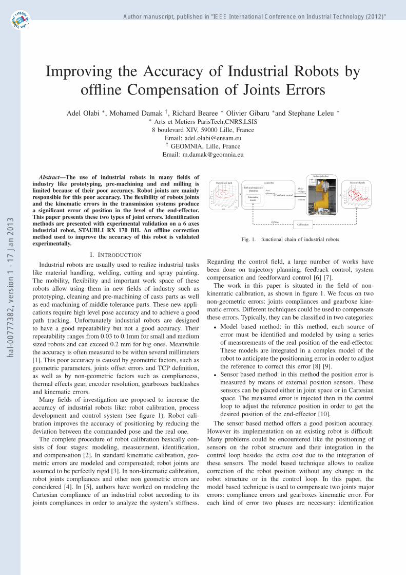
Industrial robot

Theoretical path Measured pathController

Motorvoltages

Path and trajectoryplanning Axes

950 1000 1050 1100 11500

50

100

150

199.4

199.6

199.8

200

200.2

200.4

Y [mm]

X [mm]Z

[mm

]

900 950 1000 1050 1100 11500

50

100

150

199.4

199.6

199.8

200

200.2

200.4

Y [mm]

X [mm]

Z [m

m]Feedback control

Kinematicmodel

voltages

sensors

planningreferences

X [mm]

CalibrationOff line

Fig. 1. functional chain of industrial robots

Regarding the control field, a large number of works have

been done on trajectory planning, feedback control, system

compensation and feedforward control [6] [7].

The work in this paper is situated in the field of non-

kinematic calibration, as shown in figure 1. We focus on two

non-geometric errors: joints compliances and gearboxe kine-

matic errors. Different techniques could be used to compensate

these errors. Typically, they can be classified in two categories:

• Model based method: in this method, each source of

error must be identified and modeled by using a series

of measurements of the real position of the end-effector.

These models are integrated in a complex model of the

robot to anticipate the positionning error in order to adjust

the reference to correct this error [8] [9].

• Sensor based method: in this method the position error is

measured by means of external position sensors. These

sensors can be placed either in joint space or in Cartesian

space. The measured error is injected then in the control

loop to adjust the reference position in order to get the

desired position of the end-effector [10].

The sensor based method offers a good position accuracy.

However its implementation on an existing robot is difficult.

Many problems could be encountered like the positioning of

sensors on the robot structure and their integration in the

control loop besides the extra cost due to the integration of

these sensors. The model based technique allows to realize

correction of the robot position without any change in the

robot structure or in the control loop. In this paper, the

model based technique is used to compensate two joints major

errors: compliance errors and gearboxes kinematic error. For

each kind of error two phases are necessary: identification

hal-0

0777

382,

ver

sion

1 -

17 J

an 2

013

Author manuscript, published in "IEEE International Conference on Industrial Technology (2012)"

Gea

qin Controllor

Sensor

Referecne

MotorControl

KKarbox

KK

qout

qm

Ja

Arm

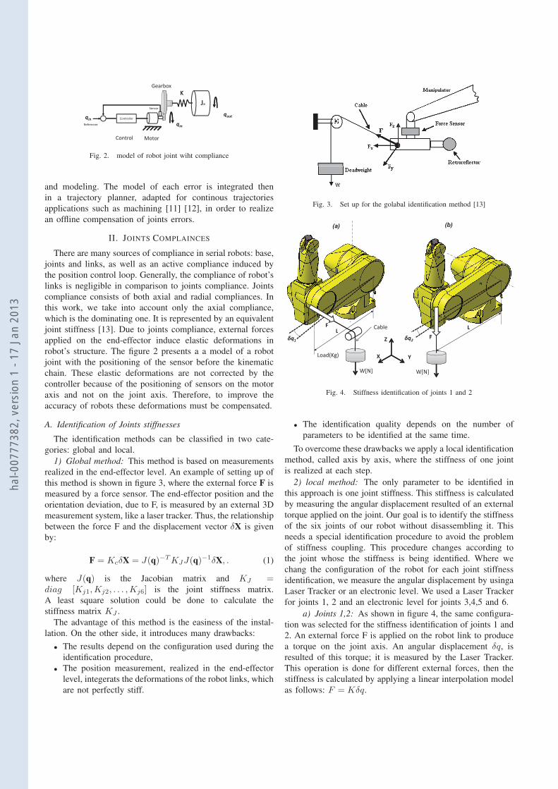
Fig. 2. model of robot joint wiht compliance

and modeling. The model of each error is integrated then

in a trajectory planner, adapted for continous trajectories

applications such as machining [11] [12], in order to realize

an offline compensation of joints errors.

II. JOINTS COMPLAINCES

There are many sources of compliance in serial robots: base,

joints and links, as well as an active compliance induced by

the position control loop. Generally, the compliance of robot’s

links is negligible in comparison to joints compliance. Joints

compliance consists of both axial and radial compliances. In

this work, we take into account only the axial compliance,

which is the dominating one. It is represented by an equivalent

joint stiffness [13]. Due to joints compliance, external forces

applied on the end-effector induce elastic deformations in

robot’s structure. The figure 2 presents a a model of a robot

joint with the positioning of the sensor before the kinematic

chain. These elastic deformations are not corrected by the

controller because of the positioning of sensors on the motor

axis and not on the joint axis. Therefore, to improve the

accuracy of robots these deformations must be compensated.

A. Identification of Joints stiffnesses

The identification methods can be classified in two cate-

gories: global and local.

1) Global method: This method is based on measurements

realized in the end-effector level. An example of setting up of

this method is shown in figure 3, where the external force F is

measured by a force sensor. The end-effector position and the

orientation deviation, due to F, is measured by an external 3D

measurement system, like a laser tracker. Thus, the relationship

between the force F and the displacement vector δX is given

by:

F = KcδX = J(q)−TKJJ(q)−1δX, . (1)

where J(q) is the Jacobian matrix and KJ =diag [Kj1,Kj2, . . . ,Kj6] is the joint stiffness matrix.

A least square solution could be done to calculate the

stiffness matrix KJ .

The advantage of this method is the easiness of the instal-

lation. On the other side, it introduces many drawbacks:

• The results depend on the configuration used during the

identification procedure,

• The position measurement, realized in the end-effector

level, integerats the deformations of the robot links, which

are not perfectly stiff.

Fig. 3. Set up for the golabal identification method [13]

(a)

FL

CableL

q1

Load(Kg) X

Z

W[N]

(b)

L

Y

Fq2

W[N]

Fig. 4. Stiffness identification of joints 1 and 2

• The identification quality depends on the number of

parameters to be identified at the same time.

To overcome these drawbacks we apply a local identification

method, called axis by axis, where the stiffness of one joint

is realized at each step.

2) local method: The only parameter to be identified in

this approach is one joint stiffness. This stiffness is calculated

by measuring the angular displacement resulted of an external

torque applied on the joint. Our goal is to identify the stiffness

of the six joints of our robot without disassembling it. This

needs a special identification procedure to avoid the problem

of stiffness coupling. This procedure changes according to

the joint whose the stiffness is being identified. Where we

chang the configuration of the robot for each joint stiffness

identification, we measure the angular displacement by usinga

Laser Tracker or an electronic level. We used a Laser Tracker

for joints 1, 2 and an electronic level for joints 3,4,5 and 6.

a) Joints 1,2: As shown in figure 4, the same configura-

tion was selected for the stiffness identification of joints 1 and

2. An external force F is applied on the robot link to produce

a torque on the joint axis. An angular displacement δq, is

resulted of this torque; it is measured by the Laser Tracker.

This operation is done for different external forces, then the

stiffness is calculated by applying a linear interpolation model

as follows: F = Kδq.

hal-0

0777

382,

ver

sion

1 -

17 J

an 2

013

q3+ q3

F

Z

q2+ q2

X Y

Fig. 5. Stiffness identification of joints 3

TABLE ISTIFFNESS OF ROBOT JOINTS

Joint N◦ 1 2 3 4 5 6

K[N.m/rad].10−6 0.204 0.85 0.57 0.49 0.12 0.005

b) Joints 3,4,5 and 6: The same strategy,

force/displacement, is applied for joints 3,4,5 and 6.

However, in the cas of joint 3 identification, the application of

an external force on the robot causes an angular displacement

in joints 2 and 3 at the same time, as shown in figure 5.

For this reason two electronic levels are necessary: one is

used as a reference to measure the angular displacement of

axis 2 according to the vertical direction and another one

to measure the combined angular displacements of joints 2

and 3. The positions of joints 2 and 3 are measured before

applying the external torque, the relative angular position

between these two joints before deformation is given by

δq = q3 − q2. After applying the force F, the new values of

the levels are q̂2 = q2 + δq2 and q̂3 = q3 + δq2 + δq3, where

δq2 and δq3 are the angular displacement of the joints. The

difference after deformation is δ̂q = q̂3 − q̂2. Thereby, the

angular displacement of joint 3 is given by:

δ̂q − δq = (q̂3 − q̂2)− (q3 − q2) ,= (q3 + δq2 + δq3 + δq2)− (q2 + δq2) ,

= δq3.(2)

The strategy is used then to measure the stiffness of joints

4,5 and 6. Figure 6 shows the positioning of the electronic

levels during the identification procedure. The table I presents

the values of the joints stiffnesses of our robot, founded by

following the previous procedure.

III. JOINTS KINEMATIC ERROR

The movement transmission in a robot joints is not ideal.

High ratio gearbox induces a kinematic error, noted qerr,

which is given by the difference between the joint anglular

position qout and the motor one qin, scaled by the ideal gear

ratio [14] as follows:

qerr =qin

gear ratio− qout. (3)

This kinematic error could limit the use of industrial robots

for high accuracy demanding applications. This error can reach

(a) q3( )

q2

q(b) q4( )

(c)

q5

Fig. 6. Levels positionning for the identification of joints 3,4 and 5

Se

1st stage:h li l

2nd stage: Jointb é bl

1 2

Motor

ensor

helical gears combiné Stäubli

Fig. 7. Joint robot transmission system

0.01◦ for each joint and generate many 1/10 of mm position

error of the end-effector. The kinematic errors are due to

defaults in the gears shape and inaccuracy in the joints and

gearsboxes components assembly.

The three first joints of our robot are equipped with two

stages of reduction system as shown in figure 7.

• The first level consists of two helical gears.

• The second level is a special reducer made by Staubli,

similar to harmonic drives.

Thus, the kinematic error of each joint is composed of

the defaults of the components of these two stages. Again,

the objective is to measure the kinematic errors without

disassembling the robot. Thereby, the identification is done

by using measurements of the positions of robot links.

c) Identification protocol : To measure the kinematic

error of a robot joint, we perform an angular displacement

of this joint. Then the real position is measured by an external

measurement system and compared to the rotary encoder com-

manded value. To avoid any dynamic effects, this operation

is done by taking measurement in static positions. Thus, the

identification of the kinematic error is done as follows:

• Measuring of the joint angular positions by an external

system, for example a Laser Tracker, in a specified

interval.

• Comparing these measures qr with the joint reference

qtheo to calculate the position error Δq = qr − qtheo.

This error cumulates the stiffness error qstiff and the

kinematic error qgear.

• Calculating the stiffness error by using robot parameters

and then extract the kinematic error.

hal-0

0777

382,

ver

sion

1 -

17 J

an 2

013

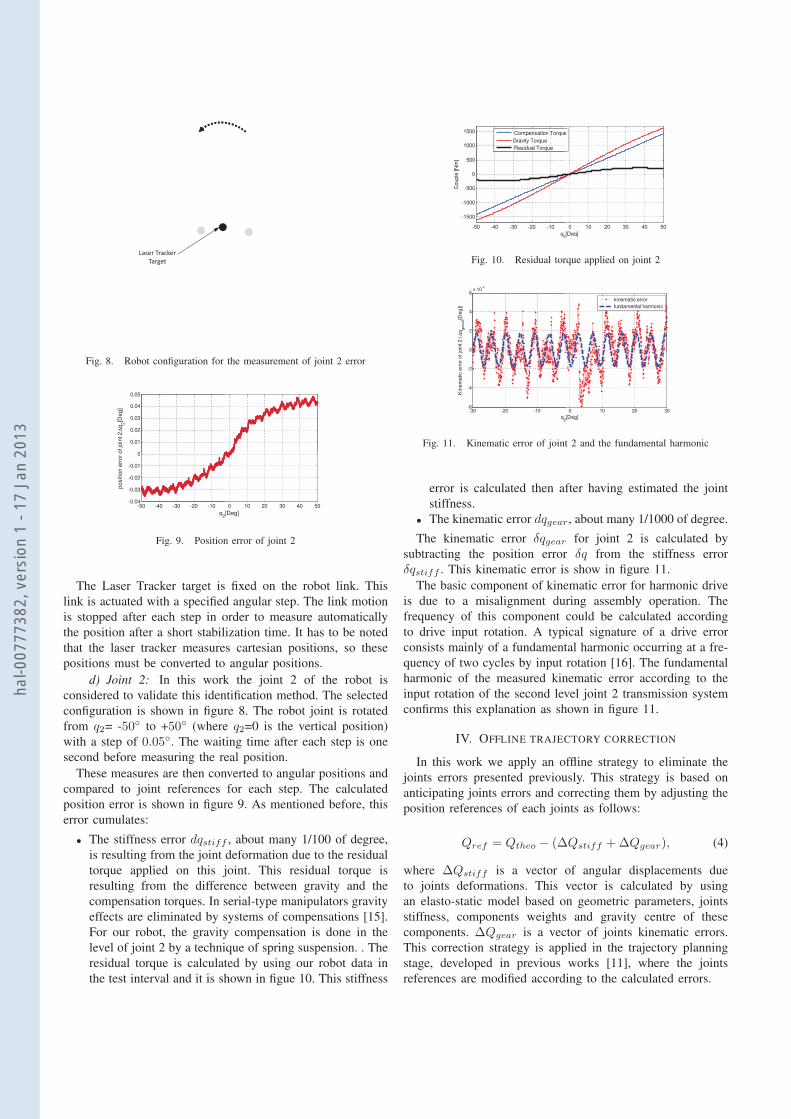
Fig. 8. Robot configuration for the measurement of joint 2 error

0

0.01

0.02

0.03

0.04

0.05

of jo

int 2

Δq 2[D

eg]

-50 -40 -30 -20 -10-0.04

-0.03

-0.02

-0.01

0

q2[

posi

tion

erro

r o

0 10 20 30 40 50[Deg]

Fig. 9. Position error of joint 2

The Laser Tracker target is fixed on the robot link. This

link is actuated with a specified angular step. The link motion

is stopped after each step in order to measure automatically

the position after a short stabilization time. It has to be noted

that the laser tracker measures cartesian positions, so these

positions must be converted to angular positions.

d) Joint 2: In this work the joint 2 of the robot is

considered to validate this identification method. The selected

configuration is shown in figure 8. The robot joint is rotated

from q2= -50◦ to +50◦ (where q2=0 is the vertical position)

with a step of 0.05◦. The waiting time after each step is one

second before measuring the real position.

These measures are then converted to angular positions and

compared to joint references for each step. The calculated

position error is shown in figure 9. As mentioned before, this

error cumulates:

• The stiffness error dqstiff , about many 1/100 of degree,

is resulting from the joint deformation due to the residual

torque applied on this joint. This residual torque is

resulting from the difference between gravity and the

compensation torques. In serial-type manipulators gravity

effects are eliminated by systems of compensations [15].

For our robot, the gravity compensation is done in the

level of joint 2 by a technique of spring suspension. . The

residual torque is calculated by using our robot data in

the test interval and it is shown in figue 10. This stiffness

0

500

1000

1500

ple

[Nm

]

Compensation TorqueGravity Torque Residual Torque

-50 -40 -30 -20 -10

-1500

-1000

-500

q2

Cou

p

e

0 10 20 30 40 50[Deg]

Fig. 10. Residual torque applied on joint 2

0

2

4

6x 10

-3

join

t 2 (

Δq g

ea

r2[D

eg])

-30 -20 -10-6

-4

-2

q2

Kin

emat

ic e

rror

of j

kinematic errorfundamental harmonic

0 10 20 30

2[Deg]

Fig. 11. Kinematic error of joint 2 and the fundamental harmonic

error is calculated then after having estimated the joint

stiffness.

• The kinematic error dqgear, about many 1/1000 of degree.

The kinematic error δqgear for joint 2 is calculated by

subtracting the position error δq from the stiffness error

δqstiff . This kinematic error is show in figure 11.

The basic component of kinematic error for harmonic drive

is due to a misalignment during assembly operation. The

frequency of this component could be calculated according

to drive input rotation. A typical signature of a drive error

consists mainly of a fundamental harmonic occurring at a fre-

quency of two cycles by input rotation [16]. The fundamental

harmonic of the measured kinematic error according to the

input rotation of the second level joint 2 transmission system

confirms this explanation as shown in figure 11.

IV. OFFLINE TRAJECTORY CORRECTION

In this work we apply an offline strategy to eliminate the

joints errors presented previously. This strategy is based on

anticipating joints errors and correcting them by adjusting the

position references of each joints as follows:

Qref = Qtheo − (ΔQstiff +ΔQgear), (4)

where ΔQstiff is a vector of angular displacements due

to joints deformations. This vector is calculated by using

an elasto-static model based on geometric parameters, joints

stiffness, components weights and gravity centre of these

components. ΔQgear is a vector of joints kinematic errors.

This correction strategy is applied in the trajectory planning

stage, developed in previous works [11], where the joints

references are modified according to the calculated errors.

hal-0

0777

382,

ver

sion

1 -

17 J

an 2

013

850900

9501000

10501100

11501200 -50

199.7

199.8

199.9

200

200.1

Z [

mm

]

050

100150

200

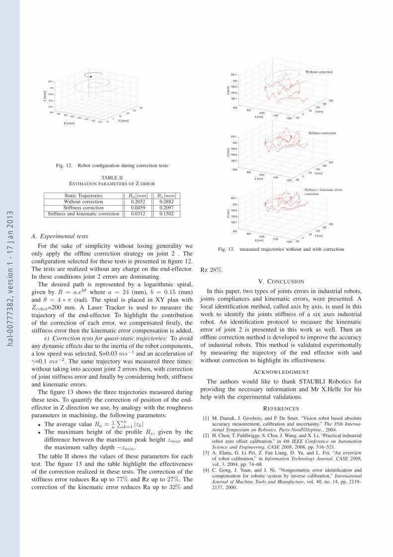
Fig. 12. Robot configuration during correction tests

TABLE IIESTIMATION PARAMETERS OF Z ERROR

Static Trajectories Ra[mm] Rz [mm]Without correction 0.2032 0.2882Stiffness correction 0.0459 0.2097

Stiffness and kinematic correction 0.0312 0.1502

A. Experimental tests

For the sake of simplicity without losing generality we

only apply the offline correction strategy on joint 2 . The

configuration selected for these tests is presented in figure 12.

The tests are realized without any charge on the end-effector.

In these conditions joint 2 errors are dominating.

The desired path is represented by a logarithmic spiral,

given by R = a.ebθ where a = 24 (mm), b = 0.15 (mm)

and θ = 4 ∗ π (rad). The spiral is placed in XY plan with

Zrobot=200 mm. A Laser Tracker is used to measure the

trajectory of the end-effector. To highlight the contribution

of the correction of each error, we compensated firstly, the

stiffness error then the kinematic error compensation is added.

e) Correction tests for quasi-static trajectories: To avoid

any dynamic effects due to the inertia of the robot components,

a low speed was selected, S=0.03 ms−1 and an acceleration of

γ=0.1 ms−2. The same trajectory was measured three times:

without taking into account joint 2 errors then, with correction

of joint stiffness error and finally by considering both, stiffness

and kinematic errors.

The figure 13 shows the three trajectories measured during

these tests. To quantify the correction of position of the end-

effector in Z direction we use, by analogy with the roughness

parameters in machining, the following parameters:

• The average value Ra = 1n

∑nk=1 |zk|

• The maximum height of the profile Rz , given by the

difference between the maximum peak height zmax and

the maximum valley depth −zmin.

The table II shows the values of these parameters for each

test. The figure 13 and the table highlight the effectiveness

of the correction realized in these tests. The correction of the

stiffness error reduces Ra up to 77% and Rz up to 27%. The

correction of the kinematic error reduces Ra up to 32% and

800900

10001100

199.7

199.8

199.9

200

200.1

X [mm]

Z [m

m]

800900

10001100

199.7

199.8

199.9

200

200.1

X [mm]

Z [m

m]

800900

10001100

199.7

199.8

199.9

200

200.1

X [mm]

Z [m

m]

1200 -500

50100

150200

Y [mm]

1200 -500

50100

150200

Y [mm]

1200 -500

50100

150200

Y [mm]

Without correction

Siffness correction

Stiffness + kinematic errorscorrection

Fig. 13. measured trajectories without and with correction

Rz 28%.

V. CONCLUSION

In this paper, two types of joints errors in industrial robots,

joints compliances and kinematic errors, were presented. A

local identification method, called axis by axis, is used in this

work to identify the joints stiffness of a six axes industrial

robot. An identification protocol to measure the kinematic

error of joint 2 is presented in this work as well. Then an

offline correction method is developed to improve the accuracy

of industrial robots. This method is validated experimentally

by measuring the trajectory of the end effector with and

without correction to highlight its effectiveness.

ACKNOWLEDGMENT

The authors would like to thank STAUBLI Robotics for

providing the necessary information and Mr X.Helle for his

help with the experimental validations.

REFERENCES

[1] M. Damak, J. Grosbois, and P. De Smet, “Vision robot based absoluteaccuracy measurement, calibration and uncertainty.” The 35th Interna-tional Symposium on Robotics. Paris-NordVillepinte., 2004.

[2] H. Chen, T. Fuhlbrigge, S. Choi, J. Wang, and X. Li, “Practical industrialrobot zero offset calibration,” in 4th IEEE Conference on AutomationScience and Engineering, CASE 2008, 2008, pp. 516–521.

[3] A. Elatta, G. Li Pei, Z. Fan Liang, D. Yu, and L. Fei, “An overviewof robot calibration,” in Information Technology Journal, CASE 2008,vol. 3, 2004, pp. 74–68.

[4] C. Gong, J. Yuan, and J. Ni, “Nongeometric error identification andcompensation for robotic system by inverse calibration,” InternationalJournal of Machine Tools and Manufacture, vol. 40, no. 14, pp. 2119–2137, 2000.

hal-0

0777

382,

ver

sion

1 -

17 J

an 2

013

[5] E. Abele, M. Weigold, and S. Rothenbcher, “Modeling and identificationof an industrial robot for machining applications,” CIRP Annals -Manufacturing Technology, vol. 56, no. 1, pp. 387–390, 2007.

[6] P. Lambrechts, M. Boerlage, and M. Steinbuch, “Trajectory planningand feedforward design for electromechanical motion systems,” ControlEngineering Practice, vol. 13, no. 2, pp. 145–157, 2005.

[7] W. B. J. Hakvoort, R. G. K. M. Aarts, J. van Dijk, and J. B. Jonker,“Lifted system iterative learning control applied to an industrial robot,”Control Engineering Practice, vol. 16, no. 4, pp. 377–391, 2008.

[8] E. Abele, S. Bauer, S. Rothenbucher, M. Stelzer, and O. von Stryk,“Prediction of the tool displacement by coupled models of the com-pliant industrial robot and the milling process,” in Proceedings of theInternational Conference on Process Machine Interactions, September2008, 2008, pp. 223–230.

[9] E. Abele, J. Bauer, M. Pischan, O. v. Stryk, M. Friedmann, andT. Hemker, “Prediction of the tool displacement for robot millingapplications using co-simulation of an industrial robot and a removalprocess,” in CIRP 2nd International Conference Process Machine Inter-actions. CIRP, jun 2010.

[10] J. Wang, H. Zhang, and T. Fuhlbrigge, “Improving machining accuracywith robot deformation compensation,” in 2009 IEEE/RSJ InternationalConference on Intelligent Robots and Systems, IROS 2009, 2009, pp.3826–3831.

[11] A. Olabi, R. Bearee, E. Nyiri, and O. Gibaru, “Enhanced trajectoryplanning for machining with industrial six-axis robots,” in Proceedingsof the IEEE International Conference on Industrial Technology, 2010,pp. 500–506.

[12] A. Olabi, R. Bare, O. Gibaru, and M. Damak, “Feedrate planningfor machining with industrial six-axis robots,” Control EngineeringPractice, vol. 18, no. 5, pp. 471–482, 2010.

[13] G. Alici and B. Shirinzadeh, “Enhanced stiffness modeling, identificationand characterization for robot manipulators,” IEEE Transactions onRobotics, vol. 21, no. 4, pp. 554–564, 2005.

[14] D. Tuttle, “Understanding and modeling the behavior of a harmonicdrive gear transmission,” Technical report, Massachusetts Institute ofTechnology, 1992.

[15] T. Wongratanaphisan and M. Chew, “Gravity compensation of spatialtwo-dof serial manipulators,” Journal of Robotic Systems, vol. 19, no. 7,pp. 329–347, 2002.

[16] F. H. Ghorbel, P. S. Gandhi, and F. Alpeter, “On the kinematic error inharmonic drive gears,” Journal of Mechanical Design, Transactions Ofthe ASME, vol. 123, no. 1, pp. 90–97, 2001.

hal-0

0777

382,

ver

sion

1 -

17 J

an 2

013