improving software project estimates based on historical data · 2018-03-15 · improving software...
TRANSCRIPT

FACULTY OF ENGINEERING OF THE UNIVERSITY OF PORTO
Improving Software Project EstimatesBased on Historical Data
Bruno Filipe Salgado Fernandes
Master in Informatics and Computing Engineering
Supervisor at FEUP: João Carlos Pascoal de Faria
Supervisor at Altran: Maria da Luz Silva Pereira dos Penedos
27th February, 2014


Improving Software Project Estimates Based onHistorical Data
Bruno Filipe Salgado Fernandes
Master in Informatics and Computing Engineering
Approved in oral examination by the committee:
Chair: Hugo José Sereno Lopes Ferreira
External Examiner: Miguel Carlos Pacheco Afonso Goulão
Supervisor: João Carlos Pascoal de Faria
27th February, 2014


Abstract
Due to the strong competition that exists in today’s markets, it is essential for a company likeAltran, to grow up further in order to be in front of both national and international level. For thisto happen, it is necessary to make good estimates in order to contract and control its projects, butsometimes in practice it isn’t always easy due to several factors. The effort estimation is a crucialstep, to determine project cost, schedule and needed resources. The estimates accuracy is decisiveboth to satisfy current customers and to attract new clients. The current work resulted from aproposal made by Altran, which set very specific and ambitious challenges in order to grow upand improve the current estimation methodology and assist project managers and respective teams.
One of the steps of the current estimation method followed by Altran involves calculatingeffort estimates for the non-development phases (analysis, testing, etc.) based on an effort estimatefor the development phase. To improve that step of the estimation process it is proposed in thisdissertation the usage of an estimation model for the percentual distribution of total project effortper phase. The estimation model is calibrated based on historical data from finished projects.
Two variants of the estimation model are proposed: a simple one, that gives estimates based ona simple averaging from past projects, and a more complex one, that requires the user to indicatethe perceived complexity (low, medium or high) of each project phase, and gives estimates of thepercentual distribution of effort per phase taking into account the historical data and the perceivedcomplexities.
Since the time to perform this dissertation was limited, the validation of the proposed modelsin future projects was not viable and as such a cross-validation method was used. The resultsshowed great potential for improving estimates, compared with the current followed method, andwith strong likelihood that eventually in the future possibly be used to achieve more ambitiousgoals.
Regarding the structure of this document, initially a problem analysis is presented and subse-quently a study is made about the state of the art. The proposed methodology and models are alsodescribed, as well as the performed validation.
In conclusion, this dissertation proposes an improvement of the estimation method followed bythe company, taking advantage of estimation best practices. It is hoped that in future projects theestimation accuracy will improve, leading to a higher satisfaction of all the involved stakeholders.
i

ii

Resumo
Devido à forte concorrência, existente nos mercados atuais, é imprescindível para uma em-presa como a Altran, evoluir ainda mais, de forma a se posicionar na frente tanto a nível nacionalcomo internacionalmente. Para que isso aconteça, é necessário fazer boas estimativas de formaa contratualizar e controlar os seus projetos, mas por vezes na prática nem sempre é fácil, dev-ido a vários fatores. A estimação do esforço torna-se uma etapa fulcral, para que seja possíveldeterminar o custo do projeto, a agenda e os recursos necessários. A precisão das estimativas édeterminante, tanto para satisfazer os atuais clientes, como para atrair novos. O presente trabalhoresultou de uma proposta feita pela Altran, que definiu desafios bem específicos e ambiciosos como objetivo de evoluir e melhorar a metodologia seguida atualmente e auxiliar os gestores de projetoe respetivas equipas.
Um dos passos do método de estimação atual seguido pela Altran envolve calcular as esti-mativas do esforço para as fases que não fazem parte do desenvolvimento (análise, testes, etc.)baseadas numa estimativa do esforço para a fase de desenvolvimento. Para melhorar este passodo processo de estimação, é proposto nesta dissertação, o uso de um modelo de estimação para adistribuição percentual do esforço total do projeto por fase. O modelo de estimação é calibradobaseado em dados históricos de projetos já finalizados.
Duas variantes do modelo de estimação são propostas: um mais simples, que fornece esti-mativas baseadas numa simples média de projetos passados, e um mais complexo, que requer aindicação da complexidade (baixa, média ou alta) de cada fase de cada projeto, e fornecer estima-tivas da distribuição percentual do esforço por fase, tendo em consideração os dados históricos eas complexidades atribuídas.
Uma vez que o tempo para a realização desta dissertação é limitado, a validação dos modelosimplementados em projetos futuros não se torna viável e como tal foi usado o método de cross-validation. Os resultados mostraram grande potencial de melhoria das estimativas, comparandocom o método seguido atualmente, e com forte probabilidade de no futuro ser possível atingirmetas mais ambiciosas.
No que diz respeito à estrutura deste documento, inicialmente é apresentada uma análise doproblema e seguidamente é feito um estudo sobre o estado da arte. É também descrita a metodolo-gia e os modelos propostos, bem como a validação efetuada.
Como conclusão, esta dissertação propõe uma melhoria do método de estimação seguido pelaempresa, aproveitando a vantagem das boas práticas de estimação. É esperado que em projetosfuturos a precisão da estimação melhore, levando a uma maior satisfação de todos os stakeholdersenvolvidos.
iii

iv
Acknowledgements
This section of my dissertation is to express my appreciation for those who over the yearswere by my side during my journey through MIEIC and who were essential for me to successfullyachieve all my goals.
First of all I would like to thank my parents, who were and are my greatest support towardsachieving my goals, and who helped in which ever situation or obstacle. I also thank them for thestability, affection and love they gave me and it is clear that without them it would be impossiblefor me to achieve all my goals.
Secondly I thank my girlfriend, Ana Luisa Oliveira Alves, a fundamental piece in my motiva-tion and inspiration along my course. I thank her for all the support and love that she has shownand I will never forget all the times we had, which were crucial for me to feel as fulfilled as I do.
To João Carlos Pascoal de Faria I thank, for the help, availability and competence demonstratedduring this project, as he was essential for the completion of this dissertation.
To Maria da Luz Silva Pereira dos Penedos, who has helped me to understand the Altransituation and the resources I will be working with, so that I can complete my dissertation, I thank.Her help was crucial so that by the end of this dissertation I can achieve improvements for thecompany.
To João Miguel Quitério, for all his help and follow up in this project. The advice and timespent were decisive so that this dissertation could meet its goals.
To António Augusto de Sousa, who as the director of MIEIC demanded rigor in every task andhas shown total availability.
To Gil Pedro da Silva for the friendship shown during these twelve years, in the good and badmoments.
To José Pedro da Fonseca Fernandes, who as my godfather, always helped me to overcome allthe barriers I encountered and always encouraged me throughout my academic course.
To Ana Mafalda Pinto dos Reis Brandão, for assisting me in this document revision.To all my friends and family in general, for all these years encouraging and helping me
throughout my difficulties. Colleagues and teachers, who witnessed all my journey and whopassed on knowledge allowing me to make it through all the challenges I encountered.
Finally, I thank the FEUP community, including the resources provided, staff and trainingengineers, who helps us become citizens with a great sense of responsibility.
Last, but not least, Altran, to all employees who contributed with their experience so thisdissertation can meet their needs.
Bruno Filipe Salgado Fernandes
v

vi

“If you want to be happy, set a goal that commands your thoughts,liberates your energy, and inspires your hopes”
Andrew Carnegie
vii

viii

Contents
1 Introduction 11.1 Context and Motivation . . . . . . . . . . . . . . . . . . . . . . . . . . . . . . . 11.2 Problem Statement and Goals . . . . . . . . . . . . . . . . . . . . . . . . . . . . 21.3 Methodology and Contributions . . . . . . . . . . . . . . . . . . . . . . . . . . 21.4 Outline . . . . . . . . . . . . . . . . . . . . . . . . . . . . . . . . . . . . . . . 3
2 Situation Analysis and Company Needs 52.1 Overview of Project Types and Management Practices at Altran Portugal . . . . . 52.2 Project Estimation at Altran Portugal . . . . . . . . . . . . . . . . . . . . . . . . 62.3 Company Needs and Ideas for Improvement . . . . . . . . . . . . . . . . . . . . 102.4 Conclusions . . . . . . . . . . . . . . . . . . . . . . . . . . . . . . . . . . . . . 10
3 State of the Art Analysis 113.1 Main Project Estimation Unexpected Problems . . . . . . . . . . . . . . . . . . 113.2 Project Estimation in the CMMI . . . . . . . . . . . . . . . . . . . . . . . . . . 12
3.2.1 CMMI for Development . . . . . . . . . . . . . . . . . . . . . . . . . . 133.2.2 Maturity Levels . . . . . . . . . . . . . . . . . . . . . . . . . . . . . . . 143.2.3 Process Areas of Maturity Level 2 . . . . . . . . . . . . . . . . . . . . . 153.2.4 Specific Goals and Practices Related with Project Estimation . . . . . . . 16
3.3 Main Project Estimation Techniques and Methods . . . . . . . . . . . . . . . . . 303.3.1 Individual Expert Judgment . . . . . . . . . . . . . . . . . . . . . . . . 303.3.2 Estimation by Analogy . . . . . . . . . . . . . . . . . . . . . . . . . . . 313.3.3 Estimation by Decomposition . . . . . . . . . . . . . . . . . . . . . . . 323.3.4 Wideband Delphi . . . . . . . . . . . . . . . . . . . . . . . . . . . . . . 323.3.5 Function Point Analysis . . . . . . . . . . . . . . . . . . . . . . . . . . 343.3.6 Proxy-Based Estimation . . . . . . . . . . . . . . . . . . . . . . . . . . 343.3.7 Constructive Cost Model . . . . . . . . . . . . . . . . . . . . . . . . . . 353.3.8 Agile Estimation . . . . . . . . . . . . . . . . . . . . . . . . . . . . . . 36
3.4 Techniques for Building and Validating Estimation Models from Historical Data . 393.4.1 Linear Regression . . . . . . . . . . . . . . . . . . . . . . . . . . . . . 393.4.2 Ordinary Least Squares . . . . . . . . . . . . . . . . . . . . . . . . . . . 423.4.3 Maximum-Likelihood Estimation . . . . . . . . . . . . . . . . . . . . . 423.4.4 Cross-Validation . . . . . . . . . . . . . . . . . . . . . . . . . . . . . . 433.4.5 Monte Carlo Method . . . . . . . . . . . . . . . . . . . . . . . . . . . . 443.4.6 Bootstrapping . . . . . . . . . . . . . . . . . . . . . . . . . . . . . . . . 45
3.5 Conclusions . . . . . . . . . . . . . . . . . . . . . . . . . . . . . . . . . . . . . 46
ix

CONTENTS
4 Model Proposal for Effort Distribution per Phase 494.1 Introduction . . . . . . . . . . . . . . . . . . . . . . . . . . . . . . . . . . . . . 494.2 Available Historical Data . . . . . . . . . . . . . . . . . . . . . . . . . . . . . . 514.3 Initial Analysis . . . . . . . . . . . . . . . . . . . . . . . . . . . . . . . . . . . 534.4 Metrics for Evaluating the Estimation Accuracy . . . . . . . . . . . . . . . . . . 564.5 Proposed Models for Estimation of the Phase Distribution . . . . . . . . . . . . . 58
4.5.1 Single-Value Model . . . . . . . . . . . . . . . . . . . . . . . . . . . . 594.5.2 Multi-Value Model . . . . . . . . . . . . . . . . . . . . . . . . . . . . . 60
4.6 Model Validation . . . . . . . . . . . . . . . . . . . . . . . . . . . . . . . . . . 634.7 Duration Impact . . . . . . . . . . . . . . . . . . . . . . . . . . . . . . . . . . . 66
5 Conclusions and Future Work 695.1 Conclusions . . . . . . . . . . . . . . . . . . . . . . . . . . . . . . . . . . . . . 695.2 Future Work . . . . . . . . . . . . . . . . . . . . . . . . . . . . . . . . . . . . . 70
References 73
A Dissertation Work Plan 77
B Altran Estimation Templates 79B.1 Altran Template for EDP Projects . . . . . . . . . . . . . . . . . . . . . . . . . 79B.2 Altran Template for Oracle Projects . . . . . . . . . . . . . . . . . . . . . . . . 81B.3 Altran Template of Data Extraction Estimates for Oracle-EBS Projects . . . . . . 85B.4 Altran Template for Change Request Estimates . . . . . . . . . . . . . . . . . . 87
x

List of Figures
2.1 EDP Template Example by Altran. . . . . . . . . . . . . . . . . . . . . . . . . . 82.2 Reference Data (simple component). . . . . . . . . . . . . . . . . . . . . . . . . 82.3 Reference Data (medium component). . . . . . . . . . . . . . . . . . . . . . . . 82.4 Reference Data (complex component). . . . . . . . . . . . . . . . . . . . . . . . 92.5 Oracle Template Example by Altran. . . . . . . . . . . . . . . . . . . . . . . . . 9
3.1 Critical Dimensions of CMMI [Tea10]. . . . . . . . . . . . . . . . . . . . . . . 133.2 CMMI Model Structure [GGK06]. . . . . . . . . . . . . . . . . . . . . . . . . . 143.3 Linear Regression. . . . . . . . . . . . . . . . . . . . . . . . . . . . . . . . . . 413.4 Okun’s Law in Macroeconomics As an Example of the Simple Linear Regression. 433.5 Monte Carlo Method Application to Determine the Lake Area. . . . . . . . . . . 453.6 Bootstrap and Smooth Bootstrap Distributions. . . . . . . . . . . . . . . . . . . 46
4.1 Proposed Estimation Methodology. . . . . . . . . . . . . . . . . . . . . . . . . . 514.2 Process Mechanism of the Models. . . . . . . . . . . . . . . . . . . . . . . . . . 584.3 Activity Diagram of Process Mechanism of the Models. . . . . . . . . . . . . . . 594.4 Correlation Between Analysis + Design Phases with Duration Variable. . . . . . 684.5 Correlation Between the Other Phases with Duration Variable. . . . . . . . . . . 68
A.1 Dissertation Work Plan. . . . . . . . . . . . . . . . . . . . . . . . . . . . . . . . 77
B.1 Cover of EDP Template. . . . . . . . . . . . . . . . . . . . . . . . . . . . . . . 79B.2 Estimates of EDP Template. . . . . . . . . . . . . . . . . . . . . . . . . . . . . 80B.3 Profiles of EDP Template. . . . . . . . . . . . . . . . . . . . . . . . . . . . . . 81B.4 Cover of Oracle Template. . . . . . . . . . . . . . . . . . . . . . . . . . . . . . 81B.5 Effort Sum of Oracle Template. . . . . . . . . . . . . . . . . . . . . . . . . . . . 81B.6 Estimates of Oracle Template. . . . . . . . . . . . . . . . . . . . . . . . . . . . 82B.7 Value Adjustment Factor of Oracle Template. . . . . . . . . . . . . . . . . . . . 83B.8 Guidelines of Oracle Template. . . . . . . . . . . . . . . . . . . . . . . . . . . . 83B.9 Reference Data of Oracle Template. . . . . . . . . . . . . . . . . . . . . . . . . 84B.10 Estimates of Oracle-EBS Template. . . . . . . . . . . . . . . . . . . . . . . . . 85B.11 Assumptions of Oracle-EBS Template. . . . . . . . . . . . . . . . . . . . . . . . 86B.12 Estimates of Change Request Template. . . . . . . . . . . . . . . . . . . . . . . 87
xi

LIST OF FIGURES
xii

List of Tables
4.1 Historical Data Provided by Altran. . . . . . . . . . . . . . . . . . . . . . . . . 524.2 Historical Data Provided by Altran After Normalization. . . . . . . . . . . . . . 524.3 Predicted Effort Percentage Per Phase. . . . . . . . . . . . . . . . . . . . . . . . 544.4 Actual Effort Percentage Per Phase. . . . . . . . . . . . . . . . . . . . . . . . . 554.5 Statistics About the Predicted Effort Percentage Per Phase. . . . . . . . . . . . . 554.6 Statistics About the Actual Effort Percentage Per Phase. . . . . . . . . . . . . . . 564.7 Initial Estimation Error of Each Phase in Each Project and Sample Total Error. . . 574.8 Single-Value Estimation Model Calibrated Based on the Available Historical Data. 604.9 Single-Value Model Total Error. . . . . . . . . . . . . . . . . . . . . . . . . . . 604.10 Multi-Value Estimation Model with T-Shirt Sizes. . . . . . . . . . . . . . . . . . 614.11 Model Calibration. . . . . . . . . . . . . . . . . . . . . . . . . . . . . . . . . . 614.12 Multi-Value Estimation Model . . . . . . . . . . . . . . . . . . . . . . . . . . . 624.13 Multi-Value Estimation Model After Normalization. . . . . . . . . . . . . . . . . 634.14 Multi-Value Model Total Error. . . . . . . . . . . . . . . . . . . . . . . . . . . . 634.15 Single-Value Model Total Error Using Cross-Validation. . . . . . . . . . . . . . 654.16 Historical Data Provided by Altran With Duration Variable. . . . . . . . . . . . . 664.17 Correlation of Each Phase of Each Project with Duration Variable. . . . . . . . . 664.18 New Correlation Dividing the Project Into Two Parts with Duration Variable. . . 67
xiii

LIST OF TABLES
xiv

Abbreviations
ADM Altran Delivery ModelCAM Capacity and Availability ManagementCAR Causal Analysis and ResolutionCM Configuration ManagementCMMI Capability Maturity Model IntegrationCMMI-ACQ CMMI for AcquisitionCMMI-DEV CMMI for DevelopmentCMMI-SVC CMMI for ServicesCOCOMO Constructive Cost ModelDAR Decision Analysis and ResolutionDISS Dissertation Curricular UnitDUnits Delivery UnitsFEUP Faculty of Engineering of the University of PortoFTE Full-time EquivalentIPM Integrated Project ManagementMA Measurement and AnalysisMIEIC Master in Informatics and Computing EngineeringOPD Organizational Process DefinitionOPF Organizational Process FocusOPM Organizational Performance ManagementOPP Organizational Process PerformanceOT Organizational TrainingPI Product IntegrationPMC Project Monitoring and ControlPP Project PlanningPPQA Process and Product Quality AssurancePROBE PROxy-Based EstimationPSP Personal Software ProcessQPM Quantitative Project ManagementRD Requirements DevelopmentREQM Requirements ManagementRSKM Risk ManagementSAM Supplier Agreement ManagementSEI Software Engineering InstituteTS Technical SolutionTSP Team Software ProcessUAT User Acceptance TestingVAL ValidationVER Verification
xv


Chapter 1
Introduction
This dissertation was prepared as part of the DISS (Dissertation Curricular Unit) of the 5th
year of the MIEIC (Master in Informatics and Computing Engineering) at FEUP (Faculty of En-
gineering of the University of Porto).
The dissertation work was accomplished in partnership with the Altran Portugal company. The
need to grow in the software engineering industry is paramount to ensure the competitiveness of
the company in such a dynamic market.
Through this document, it is possible to show some ideas about estimation models, based on
different parameters to be applied in the context of software projects.
This chapter contextualizes the problem, states the main motivation, the dissertation goals,
expected results and provides a small description of the structure of this report.
1.1 Context and Motivation
Altran is a French company, which is very significant in the market’s innovation area for nearly
thirty years. This company has more than 17,000 employees in sixteen countries, France, Ger-
many, Netherlands, Portugal, Spain, United Kingdom, Brazil, China, United States of America,
among others.
In Portugal, Altran is leader in innovation with over 400 employees and is present in multiple
activity sectors such as Financial, Telecommunications & Media, Public Administration, Industry
and Utilities. Present in Portugal since 1998, Altran has since then responded in an outstanding
manner to the market’s challenges. Altran’s headquarters in Portugal has its main focus in provid-
ing solutions and outsourcing activities. This presents a unique business model, which includes
Technological Consulting and Innovation, Organizational and Information Systems.
The mission of Altran Portugal is based on partnering with entities that contribute to the cre-
ation of innovative solutions worldwide. The employees of the group strive to the utmost, using
their skills in order to contribute to the growth of the company, which offers to the costumers the
1

Introduction
best solutions even for the most complex problems and aims at becoming a global leader in inno-
vation. "We give life to the ideas of our costumers, improve their performance through technology
and innovation" [Por13], is one of the slogans of the Altran Portugal.
Regarding the estimation of cost and effort, sometimes it is a bit more complex than it seems.
Through the estimation, the client will know how much the project will cost in terms of time and
money.
The motivation of this dissertation, results from some difficulties that exist at the moment,
regarding the estimation procedures used by Altran Portugal. In an established company such as
Altran, there are many different types of projects, and sometimes the variables that are used differ,
hence the need to create multiple models dedicated to the type of development project. To handle
such complexity a proposition was made to create a flexible estimation model based in different
parameters that support Altran’s project managers and teams in improving their effort estimates,
namely by using historical data. In this way Altran Portugal is able to position itself in the front
line and evolve with regards to high level quality standards. Leading to a higher recognition of
their projects, increase the company’s productivity and costumer relations.
1.2 Problem Statement and Goals
One of the most important stages in the life cycle of each project is the estimation of effort and
cost. Through the latter it is possible to know how much the project will cost, whether in money,
effort or even in terms of required resources to use.
With the creation of this estimation model, which takes into account the techniques used at
the time by Altran, it will be possible to improve some points in future projects. At the moment,
Altran has some models that were created with Excel tools for some projects, however they still
have some gaps. In order to overcome some points, it is intended to create a new model, but
not putting aside the existing models. The creation of this new model aims to overcome some
weaknesses of the current tool, related with the estimation accuracy and accessibility. One of
the weaknesses is that the estimation templates created by Altran embody a set of coefficients
that were defined in an ad-hoc manner and not computed from historical data. Basically, the
creation of the new flexible estimation model based in different parameters will allow support
Altran project managers and teams in improving their effort estimates, namely by using historical
data. At the moment, Altran has an estimation process that meets the requirements of CMMI
(Capability Maturity Model Integration) Level 2, in the area of Project Planning. The creation of
this model takes into account the practices of CMMI, in order to expand also to other areas.
1.3 Methodology and Contributions
This section, describes the methodology and contributions for this dissertation.
2

Introduction
The first steps explored the topic in more detail and existing solutions in order to give room
for innovation. One of the steps was to analyze the state of the art, namely estimation techniques.
Subsequently the current situation of Altran was analyzed.
Then, the historical data provided by Altran was analyzed. This allowed the implementation of
some alternatives that served of improvement of the present processes that Altran currently uses.
They went through a validation phase, by some Altran experts, which assesses if the implemented
solution could lead to a beneficial outcome for the successful development of future projects.
So, it is expected that the Altran methodology with the adjustments that were done improve
the current estimates and subsequently the future projects of this company.
1.4 Outline
Apart from the introduction, this report comprises four chapters.
Chapter 2 describes the current methodology of Altran, analyzing the points which have to
be changed and improved to meet the needs of the company and describes the CMMI model, their
practices and some features considered decisive for this dissertation work.
Chapter 3 describes the state of the art, listing estimation methods and techniques that are
crucial to build the project planning. There are also listed some techniques to build and to validate
estimation models from historical data.
Chapter 4 explains the proposed model for effort distribution per phase, where it made a pretty
short introduction and then the historical data provided by the company are presented. Finally
the model construction is described and its validation and the impact of variable duration in the
developed projects are also exposed.
Finally, in chapter 5 some conclusions are taken and points for future work are described.
3

Introduction
4

Chapter 2
Situation Analysis and Company Needs
This chapter describes the estimation process that Altran Portugal currently uses, in order to
identify its strengths, weaknesses and improvement opportunities.
2.1 Overview of Project Types and Management Practices at AltranPortugal
Altran Portugal reached the maturity level 2 in the CMMI DEV 1.3 model for Development, in
2012. This reference model certifies skills in information technologies, for products and services
development applied in software engineering and systems areas [CKS11].
After acquiring this certification, Altran aims to ensure that the four axes of evaluation - time,
budget, scope and quality, are recognized in the commitments undertaken in projects of their
clients. Achieving this maturity level is aligned with the continuous improvement that Altran has
shown in their services.
The main advantages of having attained this level can be summarized in [CKS11]:
• Improved product quality due to more rigorous processes and better requirements gathering;
• Greater projects predictability;
• Increased credibility in the market;
• Due to the rigor of certification audits, CMMI creates greater competitiveness, since the
presented proposals are more competitive at budget level, by allowing projects to have more
accurate estimate.
The ADM (Altran Delivery Model) consists in four steps, Consultancy & Technical Support,
Competences: Team of Managed Consultants, Projects that focus on Fixed Price Commitments
and finally Outsourced Services. Just steps Fixed Price Commitments and Outsourced Services
5

Situation Analysis and Company Needs
involve estimates. The remaining steps are based on analysing Competences and Skills Com-
mitment. Regarding Fixed Price phase, who is usually called ADM3 sometimes there may be
change requests, which are some extras that the customer or the company think to be relevant to
the project, but in the initial phase were not mentioned. After creating this request the impact is
analysed to determine what this change will have on the project, the alternatives are studied and
the decision if this change is accepted or not. If the request was accepted, the project planning
is revised, implements the change request, validating the change and closes the change request.
If it wasn’t accepted, the change is not implemented and closes the change request. Regarding
Outsourced Services, called for ADM4, these can sometimes be project updates that the company
made for a client, or may also include projects that the customer bought to another client and can
be reformulated by Altran, or start since the beginning of respective project if they feel that it is
impractical to continue the project done so far.
To establish contact with the company, it was noticed that on the current situation, worksheets
are used to estimate effort, before the project starts, then the project is divided into features /
work items whose effort is estimated individually and finally is coupled and distributed by project
phases. Besides that, have effort deviation data and have diary effective effort registration. For
tools that use this time, there is the Clarity at group level, Jira-Issues, Project, Excel, among others.
They also use an open source system, which is the Knowledge Tree that allows an organization to
manage and securely share their documents.
2.2 Project Estimation at Altran Portugal
Altran is currently "certified" at CMMI Level 2, in the area of project planning. The idea is to
analyze the effort estimation of projects, which subsequently also examines the cost and schedule,
which will be calculated according to effort.
At this point, in order to be able to make estimates in various types of projects, Altran has been
using spreadsheets for several built models, in accordance with the parameters required for each
project. Effort is calculated based on the parameters indicated and is represented in the form of
"function points". This conversion is adjusted for the different projects, with the results obtained
at the completion of each project.
When estimates are made for certain projects, data from past projects is taken into account
in order to estimate more correctly based on experience, provided that there is data about the
company or client to which Altran is developing a specific project. Furthermore, Altran, convenes
meetings with various experts in the software projects area, to discuss the various estimates, a
method that is very similar to the method of Wideband Delphi (see section 3.3.4).
By analyzing the data provided by Altran, the methodology currently used was shown to es-
timate the various projects. There are templates for Oracle estimating projects, for example. The
model should be refined in order to adapt to different types of projects, trying to build a model that
is unique, enabling estimation for any type of project. Altran employees agree that estimating each
6

Situation Analysis and Company Needs
type of project with a unique model is not always an easy task, since it can sometimes cause con-
flicts due to certain variables and as a continuous process is not followed. Sometimes the current
method takes several changes, which causes much loss of time to improve and to adapt to different
models. They also agree that when using estimation methods, the results may significantly help to
develop quality projects.
Currently, Altran has estimation models that respond to most of the company’s needs, mainly
relying on the knowledge of experts in the field of software engineering.
In order to make the units of measurement more generic, it was thought to use DUnits (De-
livery Units) instead of calculating directly the effort in the form of (man*day). Thus, these units
will be refined over time and will make the estimation process easier and the results will be more
consistent.
Altran’s projects, are more than software development projects, since consulting, customizing
solutions, training, among others activities are central to the success of a company. Sometimes the
estimation methods and techniques fail to respond in an acceptable manner to all these activities.
Some of the templates used to estimate some types of projects are shown in Figure 2.1 through
Figure 2.5. In Figure 2.1, it is possible to see the various phases that make up the project; the per-
centage is calculated based on Development phase. The total number of FTEs (Full-time Equiva-
lent) are twenty. In the Development phase, ten FTEs were assigned, hence the 50% slice of the
pie chart. For example, in the Analysis phase, as 20% of Development phase, then to calculate the
number of FTEs becomes 0.2*10 = 2 FTEs. Then this value is converted according to the total
number of FTEs and the resulting slice of 10% as can be seen by the graph. The only stage that in
not calculated according to the development phase is Project Management.
Regarding Figure 2.5, it can be seen that there is a reference table for different types of com-
ponents that can be classified as simple, medium and complex. The spreadsheet shows the number
of components of each feature, with the degree of complexity desired. For example, if there is a
simple component in layout functionality, the result is four hours, which is the estimated time in
the reference table as can be seen in Figure 2.2. This value is set automatically by the spreadsheet,
based on the reference table.
These were only a few templates that Altran shared, but there are many more. More details
about Altran templates are shown in appendix B.
7

Situation Analysis and Company Needs
Figure 2.1: EDP Template Example by Altran.
Figure 2.2: Reference Data (simple component).
Figure 2.3: Reference Data (medium component).
8

Situation Analysis and Company Needs
Figure 2.4: Reference Data (complex component).
Figure 2.5: Oracle Template Example by Altran.
9

Situation Analysis and Company Needs
2.3 Company Needs and Ideas for Improvement
Initially, some parameters were collected that will determine the complexity of the project,
such as the type of customer, size of the project, among others. These parameters will influence
the calculation of the effort that will be estimated later.
The Pre-Sale is estimated at the lowest level all the project requirements being evaluated are
described. If the project is approved, the staff of After-Sale will estimate again and reshape so
that the project to be developed is the closest to what the client has in mind, so that it is satisfied
with the work developed. Then follows the execution, to which a deviation percentage (risk) is
assigned, in relation to the estimation made earlier. Next, the templates are used for the type of
project to develop, and at the end we arrive at a result.
Although this methodology is interesting it is not always correct since the deviations given,
may condition a little bit the reality of the estimates that were made to the respective project. As
such, it is intended to include a new step between the execution step and the end of the current
methodology, which will be made a process analysis and feedback. More specifically, through
historical data, provided by Altran Portugal we should set up and apply feedback mechanisms
with adjustment coefficients, before using the templates for each type of project. Some metrics
may also be changed during the execution and may also be changed or improved some templates
for some types of projects, in order to get a result that is more consistent.
Regarding the studied techniques, they can take the advantage of historical data provided by
the company, and from that obtain improvements through speed as in agile methods, PROBE
(Proxy-Based Estimation) (see section 3.3.6), Function Point Analysis (see section 3.3.5), among
others. Other improvements that could be made are that a greatness that is not effort as story
points, function points, use case points, architecture based sizing, among others. May also be used
corrective factors based on risk and project characteristics, through the COCOMO (Constructive
Cost Model) method (see section 3.3.7).
2.4 Conclusions
In conclusion, the estimation model to create may be based on current methodology, where
it will be refined according to the historical data available from previous projects, leading to a
significant improvement of the Altran estimation process. CMMI processes should be taken into
account not to affect the quality of projects to develop and to lead to an increased process maturity
level.
10

Chapter 3
State of the Art Analysis
Project estimation is called "The Black Art" [McC06], since it is too complex and imprecise
in practice, although theoretically it may seem trivial. For an expert to estimate a specific project,
it is not as difficult as people think, but some aspects should be taken in mind.
The result of project estimation is the project cost, schedule and needed resources. It should
also be taken into account the size of the project to develop and what it involves, how to include
software development or any personalization solution that already exists.
This chapter aims to describe the estimation methods and techniques, which are more utilized
for this type of problems, and compare their main advantages and disadvantages.
3.1 Main Project Estimation Unexpected Problems
When someone is estimating a project, some unexpected problems can happen, some more
relevant than others. Here are some of those problems: [McC06]
• Lack of historical data;
• The scope of the project changes later, after the estimation phase was closed;
• Lack of people with experience in software engineering area, in order to estimate some
tasks, time spent unnecessarily in meetings, consultancy, among others;
• The manager does not approve the initial estimate;
• At one point in the project, losing some team members, being necessary to request other
elements that will need training in a very short period;
• A new technology may emerge in the market which will facilitate the entire development of
the product or service to be developed;
• Requirements change.
11

State of the Art Analysis
3.2 Project Estimation in the CMMI
The CMMI is a reference model that contains practices that may be general or specific for
some process areas. These lead to maturity in areas such as software engineering, for example.
These practices allow the improvement of processes for the products development and services.
Briefly, it encompasses the best practices that cover the product lifecycle, from its conception to
delivery and maintenance [CKS11]. The CMMI is divided into three models, CMMI-DEV (CMMI
for Development), CMMI-ACQ (CMMI for Acquisition) and CMMI-SVC (CMMI for Services).
This dissertation will only focus on the CMMI-DEV model [God13]. The CMMI-DEV contains
twenty-two process areas.
Regarding to best practices for software projects, including cost estimation, must follow cer-
tain crucial practices to project success. When we have a project that has about 10,000 function
points or more is a bit more complicated to estimate, as such will need to follow some best prac-
tices like:
• Trained estimating specialists;
• Inclusion of new and changing requirements in the estimate;
• Quality estimation as well as schedule and cost estimation;
• Estimation of all project management tasks;
• Sufficient historical benchmark data to defend an estimate against arbitrary changes;
• Risk prediction and Analysis;
• Inclusion of reusable materials in estimates;
• Comparison of estimates to historical benchmark data from similar projects;
• Software Estimation Tools (CHECKPOINT, COCOMO, KnowledgePlan, Price-S, SLIM,
SoftCost, among others);
• Estimation of plans, specifications, and tracking costs [Jon09].
When an organization adopts the CMMI model, it may have many advantages, among which
stands out the improvement of the quality of their products, which in turn will improve the projects’
performance [GGK06]. Nowadays, due to high competition between companies, these have in-
creased interest in offering to customers, products and services with a lower delivery time with
higher quality at lower costs. Companies have been building products with a higher level of com-
plexity. The company doesn’t always develop all components of a final product. Sometimes, a
company gets some of those components from suppliers and so, together with the components
developed by them, the company reaches a final product or service.
12

State of the Art Analysis
Some organizations develop enterprise solutions and as such, an effective assets management
will be crucial in order to succeed in business area. In order to successfully meet all their goals,
these organizations require an integrated approach in development activities, thus achieving com-
plete the products and services which they set themselves to achieve [CKS11].
Figure 3.1 shows the three dimensions where organizations typically focus on.
Figure 3.1: Critical Dimensions of CMMI [Tea10].
3.2.1 CMMI for Development
CMMI for Development aims to helping organizations improving their development and main-
tenance processes for their products and services. This model brings together a set of best practices
that originate from the CMMI framework. This section describes CMMI for development version
1.3.
The CMMI approach enables process improvement and evaluations, through two different
representations: continuous and staged [CKS11]. These representations enable an organization to
use different approaches to improve according with their interest. The first representation allows
an organization to select a process area or several areas and improve the processes related with that
specific area. It is used for a single process area or selected set of process areas [GGK06]. The
second provides a standard sequence of improvements, serving as a basis for maturity comparisons
between projects and organizations. It is used for a pre-defined set of process areas across an
organization [GGK06].
13

State of the Art Analysis
Figure 3.2: CMMI Model Structure [GGK06].
3.2.2 Maturity Levels
Each maturity level consists of specific and generic practices, which relate to a predefined set
of process areas that aim at improving the overall performance of an organization. Through the
maturity level, it is possible to predict the performance of an organization in a given area or in a
group of areas.
A maturity level is a well-defined evolutionary plateau toward achieving a mature software
process. These levels solidify an organization’s processes in order to prepare that part for the next
maturity level. In order to know when it reaches the next level, it is required to check the goals
that have been met in each set of each process area [CKS11].
There are five maturity levels where each layer specifies the improvement of the current pro-
cess:
1. Initial (ad hoc)At the first maturity level, processes are usually ad hoc and chaotic. In this layer there aren’t
process areas. The organization usually does not provide a stable environment to support the
processes. Some characteristics of the organizations that are at this level is that they tend to
abandon processes in a crisis time and are also characterized by an inability to repeat their
successes [CKS11].
2. ManagedAt the second maturity level, the organization’s projects ensure that processes are planned
and executed in accordance with the stipulated policy. Are monitored, reviewed and evalu-
ated. The process areas of this layer are REQM (Requirements Management), PP (Project
14

State of the Art Analysis
Planning), PMC (Project Monitoring and Control), SAM (Supplier Agreement Manage-
ment), MA (Measurement and Analysis), PPQA (Process and Product Quality Assurance)
and CM (Configuration Management). They will be explained in more detail in section 3.2.3.
The products and services meet the specific descriptions of the process and respective pro-
cedures [CKS11].
3. DefinedAt the third maturity level, processes are well characterized and understood, and are de-
scribed in standards, procedures, tools and methods. The difference between the level 2
(Managed) and level 3 (Defined) relates to the scope of standards, processes descriptions and
procedures in this layer the processes are usually described with a higher accuracy level. The
process areas of this level are RD (Requirements Development), TS (Technical Solution),
PI (Product Integration), VER (Verification), VAL (Validation), OPF (Organizational Pro-
cess Focus), OPD (Organizational Process Definition), OT (Organizational Training), IPM
(Integrated Project Management), RSKM (Risk Management) and DAR (Decision Analysis
and Resolution) [CKS11].
4. Quantitatively ManagedAt the fourth maturity level, the organization and projects establish quantitative goals of
quality and process performance, using them as criteria in managing processes. The process
areas at this level are OPP (Organizational Process Performance) and QPM (Quantitative
Project Management). The performance of quality and processes is understood in statistical
terms and is managed throughout the processes life [CKS11].
5. OptimizingIn the fifth and final maturity level, an organization continually improves their processes
based on a quantitative understanding of the common causes of variation inherent in pro-
cesses. Process areas of this layer are the OPM (Organizational Performance Management)
and CAR (Causal Analysis and Resolution) [CKS11].
3.2.3 Process Areas of Maturity Level 2
The process areas that make up each level of maturity correspond to aspects in the development
of a product or even areas of an organization that will implement the CMMI practices.
Each maturity level consists of different process areas that have goals to meet. Below are
presented, the areas that are part of the maturity level 2 of CMMI.
• REQM - Requirements ManagementThe purpose of the Requirements Management area is to manage products requirements of
15

State of the Art Analysis
the projects and the product components, identifying some inconsistencies between those
requirements and the project plans and work products. Furthermore it also ensures that all
requirements are met and that they meet the expectations of stakeholders [CKS11].
• PP - Project PlanningThe Project Planning area is responsible to establish and maintain plans that define the
activities in the project scope. The requirements and the tasks that must be met are defined
in project planning as well as the necessary resources [CKS11].
• PMC - Project Monitoring and ControlThe purpose of the Project Monitoring and Control is to provide an understanding of the
project progress, so that it can be possible to take appropriate corrective actions when the
project’s performance deviates significantly from the established plan. The great importance
for an organization is that despite having a good preparation, often in practice it is hard to
avoid that have deviations from the plan [CKS11].
• SAM - Supplier Agreement ManagementThe Supplier Agreement Management aims to manage the products acquisition from sup-
pliers. To minimize the projects risk, and beyond cope with products and services, also
manages the support tools to the development and maintenance of these projects [CKS11].
• MA - Measurement and AnalysisThe purpose of the Measurement and Analysis area is to develop and sustain a measurement
capability that is used to support the information management needs. This information
allows estimating how the data influence the actions and the plans of the organization in a
project [CKS11].
• PPQA - Process and Product Quality AssuranceThe Process and Product Quality Assurance area aims to provide staff and management with
objective insight into processes and associated work products. Quality assurance should
begin in the project early stages to establish plans, processes, standards and procedures
that add value the project and meet the project requirements and organizational policies
[CKS11].
• CM - Configuration ManagementThe purpose of the Configuration Management area is to establish and maintain the integrity
of work products using configuration identification, configuration control, configuration sta-
tus accounting and configuration audits [CKS11].
3.2.4 Specific Goals and Practices Related with Project Estimation
There are two categories of goals and practices: generic and specific. Specific goals and prac-
tices are specific to a process area. Generic goals and practices are a part of every process area. A
16
State of the Art Analysis
process area is satisfied when organizational processes cover all of the generic and specific goals
and practices for that process area [Tea10].
Generic Goals and Practices
Generic goals and practices are a part of every process area.
• GG 1 Achieve Specific Goals
– GP 1.1 Perform Specific Practices
• GG 2 Institutionalize a Managed Process
– GP 2.1 Establish an Organizational Policy
– GP 2.2 Plan the Process
– GP 2.3 Provide Resources
– GP 2.4 Assign Responsibility
– GP 2.5 Train People
– GP 2.6 Control Work Products
– GP 2.7 Identify and Involve Relevant Stakeholders
– GP 2.8 Monitor and Control the Process
– GP 2.9 Objectively Evaluate Adherence
– GP 2.10 Review Status with Higher Level Management
• GG 3 Institutionalize a Defined Process
– GP 3.1 Establish a Defined Process
– GP 3.2 Collect Process Related Experiences
Specific Goals and Practices
Each process area is defined by a set of goals and practices. These goals and practices appear
only in that process area.
Process Areas
CAM (Capacity and Availability Management)
A Support process area at Maturity Level 3.
17
State of the Art Analysis
The purpose of CAM is to ensure effective service system performance and ensure that re-
sources are provided and used effectively to support service requirements.
Specific Practices by Goal
• SG 1 Prepare for Capacity and Availability Management
– SP 1.1 Establish a Capacity and Availability Management Strategy
– SP 1.2 Select Measures and Analytic Techniques
– SP 1.3 Establish Service System Representations
• SG 2 Monitor and Analyze Capacity and Availability
– SP 2.1 Monitor and Analyze Capacity
– SP 2.2 Monitor and Analyze Availability
– SP 2.3 Report Capacity and Availability Management Data
CAR
A Support process area at Maturity Level 5.
The purpose of CAR is to identify causes of selected outcomes and take action to improve
process performance.
Specific Practices by Goal
• SG 1 Determine Causes of Selected Outcomes
– SP 1.1 Select Outcomes for Analysis
– SP 1.2 Analyze Causes
• SG 2 Address Causes of Selected Outcomes
– SP 2.1 Implement Action Proposals
– SP 2.2 Evaluate the Effect of Implemented Actions
– SP 2.3 Record Causal Analysis Data
CM
A Support process area at Maturity Level 2.
The purpose of CM is to establish and maintain the integrity of work products using configura-
tion identification, configuration control, configuration status accounting, and configuration audits.
Specific Practices by Goal
18

State of the Art Analysis
• SG 1 Establish Baselines
– SP 1.1 Identify Configuration Items
– SP 1.2 Establish a Configuration Management System
– SP 1.3 Create or Release Baselines
• SG 2 Track and Control Changes
– SP 2.1 Track Change Requests
– SP 2.2 Control Configuration Items
• SG 3 Establish Integrity
– SP 3.1 Establish Configuration Management Records
– SP 3.2 Perform Configuration Audits
DAR
A Support process area at Maturity Level 3.
The purpose of DAR is to analyze possible decisions using a formal evaluation process that
evaluates identified alternatives against established criteria.
Specific Practices by Goal
• SG 1 Evaluate Alternatives
– SP 1.1 Establish Guidelines for Decision Analysis
– SP 1.2 Establish Evaluation Criteria
– SP 1.3 Identify Alternative Solutions
– SP 1.4 Select Evaluation Methods
– SP 1.5 Evaluate Alternative Solutions
– SP 1.6 Select Solutions
IPM
A process area at Maturity Level 3.
The purpose of IPM is to establish and manage the project and the involvement of relevant
stakeholders according to an integrated and defined process that is tailored from the organization’s
set of standard processes.
Specific Practices by Goal
19

State of the Art Analysis
• SG 1 Use the Project’s Defined Process
– SP 1.1 Establish the Project’s Defined Process
– SP 1.2 Use Organizational Process Assets for Planning Project Activities
– SP 1.3 Establish the Project’s Work Environment
– SP 1.4 Integrate Plans
– SP 1.5 Manage the Project Using the Integrated Plans
– SP 1.6 Contribute to Organizational Process Assets
• SG 2 Coordinate and Collaborate with Relevant Stakeholders
– SP 2.1 Manage Stakeholder Involvement
– SP 2.2 Manage Dependencies
– SP 2.3 Resolve Coordination Issues
MA
A Support process area at Maturity Level 2.
The purpose of MA is to develop and sustain a measurement capability used to support man-
agement information needs.
Specific Practices by Goal
• SG 1 Align Measurement and Analysis Activities
– SP 1.1 Establish Measurement Objectives
* Resources, People, Facilities and Techniques.
– SP 1.2 Specify Measures
* Information Needs Document, Guidance, Reference and Reporting.
– SP 1.3 Specify Data Collection and Storage Procedures
* Sources, Methods, Frequency and Owners.
– SP 1.4 Specify Analysis Procedures
* Rules, Alarms, SPC and Variance.
• SG 2 Provide Measurement Results
– SP 2.1 Obtain Measurement Data
* Actual, Plan, Automatic and Manual.
– SP 2.2 Analyze Measurement Data
20

State of the Art Analysis
* Evaluate, Drill Down and RCA.
– SP 2.3 Store Data and Results
* Store, Secure, Accessible, History and Evidence.
– SP 2.4 Communicate Results
* Information Sharing, Dash Boards, Up to Date, Simple and Interpret.
OPD
A process area at Maturity Level 3.
The purpose of OPD is to establish and maintain a usable set of organizational process assets,
work environment standards, and rules and guidelines for teams.
Specific Practices by Goal
• SG 1 Establish Organizational Process Assets
– SP 1.1 Establish Standard Processes
– SP 1.2 Establish Lifecycle Model Descriptions
– SP 1.3 Establish Tailoring Criteria and Guidelines
– SP 1.4 Establish the Organization’s Measurement Repository
– SP 1.5 Establish the Organization’s Process Asset Library
– SP 1.6 Establish Work Environment Standards
– SP 1.7 Establish Rules and Guidelines for Teams
OPF
A process area at Maturity Level 3.
The purpose of OPF is to plan, implement, and deploy organizational process improvements
based on a thorough understanding of current strengths and weaknesses of the organization’s pro-
cesses and process assets.
Specific Practices by Goal
• SG 1 Determine Process Improvement Opportunities
– SP 1.1 Establish Organizational Process Needs
– SP 1.2 Appraise the Organization’s Processes
– SP 1.3 Identify the Organization’s Process Improvements
• SG 2 Plan and Implement Process Improvements
21

State of the Art Analysis
– SP 2.1 Establish Process Action Plans
– SP 2.2 Implement Process Action Plans
• SG 3 Deploy Organizational Process Assets and Incorporate Experiences
– SP 3.1 Deploy Organizational Process Assets
– SP 3.2 Deploy Standard Processes
– SP 3.3 Monitor the Implementation
– SP 3.4 Incorporate Experiences into Organizational Process Assets
OPM
A process area at Maturity Level 5.
The purpose of OPM is to proactively manage the organization’s performance to meet its busi-
ness objectives.
Specific Practices by Goal
• SG 1 Manage Business Performance
– SP 1.1 Maintain Business Objectives
– SP 1.2 Identify and Analyze Innovations
– SP 1.3 Analyze Process Performance Data
• SG 2 Select Improvements
– SP 2.1 Elicit Suggested Improvements
– SP 2.2 Analyze Suggested Improvements
– SP 2.3 Validate Improvements
– SP 2.4 Select and Implement Improvements for Deployment
• SG 3 Deploy Improvements
– SP 3.1 Plan the Deployment
– SP 3.2 Manage the Deployment
– SP 3.3 Evaluate Improvement Effects
OPP
A process area at Maturity Level 4.
The purpose of OPP is to establish and maintain a quantitative understanding of the perfor-
mance of selected processes in the organization’s set of standard processes in support of achieving
22

State of the Art Analysis
quality and process performance objectives, and to provide process performance data, baselines,
and models to quantitatively manage the organization’s projects.
Specific Practices by Goal
• SG 1 Establish Performance Baselines and Models
– SP 1.1 Establish Quality and Process Performance Objectives
– SP 1.2 Select Processes
– SP 1.3 Establish Process Performance Measures
– SP 1.4 Analyze Process Performance and Establish Process Performance Baselines
– SP 1.5 Establish Process Performance Models
OT
A process area at Maturity Level 3.
The purpose of OT is to develop skills and knowledge of people so they can perform their roles
effectively and efficiently.
Specific Practices by Goal
• SG 1 Establish an Organizational Training Capability
– SP 1.1 Establish Strategic Training Needs
– SP 1.2 Determine Which Training Needs Are the Responsibility of the Organization
– SP 1.3 Establish an Organizational Training Tactical Plan
– SP 1.4 Establish a Training Capability
• SG 2 Provide Training
– SP 2.1 Deliver Training
– SP 2.2 Establish Training Records
– SP 2.3 Assess Training Effectiveness
PI
An Engineering process area at Maturity Level 3.
The purpose of PI is to assemble the product from the product components, ensure that the
product, as integrated, behaves properly (i.e., possesses the required functionality and quality at-
tributes), and deliver the product.
Specific Practices by Goal
23

State of the Art Analysis
• SG 1 Prepare for Product Integration
– SP 1.1 Establish an Integration Strategy
– SP 1.2 Establish the Product Integration Environment
– SP 1.3 Establish Product Integration Procedures and Criteria
• SG 2 Ensure Interface Compatibility
– SP 2.1 Review Interface Descriptions for Completeness
– SP 2.2 Manage Interfaces
• SG 3 Assemble Product Components and Deliver the Product
– SP 3.1 Confirm Readiness of Product Components for Integration
– SP 3.2 Assemble Product Components
– SP 3.3 Evaluate Assembled Product Components
– SP 3.4 Package and Deliver the Product or Product Component
PMC
A process area at Maturity Level 2.
The purpose of PMC is to provide an understanding of the project’s progress so that appropri-
ate corrective actions can be taken when the project’s performance deviates significantly from the
plan.
Specific Practices by Goal
• SG 1 Monitor the Project Against the Plan
– SP 1.1 Monitor Project Planning Parameters
– SP 1.2 Monitor Commitments
– SP 1.3 Monitor Project Risks
– SP 1.4 Monitor Data Management
– SP 1.5 Monitor Stakeholder Involvement
– SP 1.6 Conduct Progress Reviews
– SP 1.7 Conduct Milestone Reviews
• SG 2 Manage Corrective Action to Closure
– SP 2.1 Analyze Issues
– SP 2.2 Take Corrective Action
24

State of the Art Analysis
– SP 2.3 Manage Corrective Actions
PP
A process area at Maturity Level 2.
The purpose of PP is to establish and maintain plans that define project activities.
Specific Practices by Goal
• SG 1 Establish Estimates
– SP 1.1 Estimate the Scope of the Project
– SP 1.2 Establish Estimates of Work Product and Task Attributes
– SP 1.3 Define Project Lifecycle Phases
– SP 1.4 Estimate Effort and Cost
• SG 2 Develop a Project Plan
– SP 2.1 Establish the Budget and Schedule
– SP 2.2 Identify Project Risks
– SP 2.3 Plan Data Management
– SP 2.4 Plan the Project’s Resources
– SP 2.5 Plan Needed Knowledge and Skills
– SP 2.6 Plan Stakeholder Involvement
– SP 2.7 Establish the Project Plan
• SG 3 Obtain Commitment to the Plan
– SP 3.1 Review Plans that Affect the Project
– SP 3.2 Reconcile Work and Resource Levels
– SP 3.3 Obtain Plan Commitment
PPQA
A Support process area at Maturity Level 2.
The purpose of PPQA is to provide staff and management with objective insight into processes
and associated work products.
Specific Practices by Goal
• SG 1 Objectively Evaluate Processes and Work Products
25

State of the Art Analysis
– SP 1.1 Objectively Evaluate Processes
– SP 1.2 Objectively Evaluate Work Products
• SG 2 Provide Objective Insight
– SP 2.1 Communicate and Resolve Noncompliance Issues
– SP 2.2 Establish Records
QPM
A process area at Maturity Level 4.
The purpose of the QPM process area is to quantitatively manage the project to achieve the
project’s established quality and process performance objectives.
Specific Practices by Goal
• SG 1 Prepare for Quantitative Management
– SP 1.1 Establish the Project’s Objectives
– SP 1.2 Compose the Defined Processes
– SP 1.3 Select Subprocesses and Attributes
– SP 1.4 Select Measures and Analytic Techniques
• SG 2 Quantitatively Manage the Project
– SP 2.1 Monitor the Performance of Selected Subprocesses
– SP 2.2 Manage Project Performance
– SP 2.3 Perform Root Cause Analysis
RD
An Engineering process area at Maturity Level 3.
The purpose of RD is to elicit, analyze, and establish customer, product, and product compo-
nent requirements.
Specific Practices by Goal
• SG 1 Develop Customer Requirements
– SP 1.1 Elicit Needs
– SP 1.2 Transform Stakeholder Needs into Customer Requirements
• SG 2 Develop Product Requirements
26

State of the Art Analysis
– SP 2.1 Establish Product and Product Component Requirements
– SP 2.2 Allocate Product Component Requirements
– SP 2.3 Identify Interface Requirements
• SG 3 Analyze and Validate Requirements
– SP 3.1 Establish Operational Concepts and Scenarios
– SP 3.2 Establish a Definition of Required Functionality and Quality Attributes
– SP 3.3 Analyze Requirements
– SP 3.4 Analyze Requirements to Achieve Balance
– SP 3.5 Validate Requirements
REQM
A process area at Maturity Level 2.
The purpose of REQM is to manage requirements of the project’s products and product com-
ponents and to ensure alignment between those requirements and the project’s plans and work
products.
Specific Practices by Goal
• SG 1 Manage Requirements
– SP 1.1 Understand Requirements
– SP 1.2 Obtain Commitment to Requirements
– SP 1.3 Manage Requirements Changes
– SP 1.4 Maintain Bidirectional Traceability of Requirements
– SP 1.5 Ensure Alignment Between Project Work and Requirements
RSKM
A process area at Maturity Level 3.
The purpose of RSKM is to identify potential problems before they occur so that risk handling
activities can be planned and invoked as needed across the life of the product or project to mitigate
adverse impacts on achieving objectives.
Specific Practices by Goal
• SG 1 Prepare for Risk Management
– SP 1.1 Determine Risk Sources and Categories
27

State of the Art Analysis
– SP 1.2 Define Risk Parameters
– SP 1.3 Establish a Risk Management Strategy
• SG 2 Identify and Analyze Risks
– SP 2.1 Identify Risks
– SP 2.2 Evaluate, Categorize, and Prioritize Risks
• SG 3 Mitigate Risks
– SP 3.1 Develop Risk Mitigation Plans
– SP 3.2 Implement Risk Mitigation Plans
SAM
A process area at Maturity Level 2.
The purpose of SAM is to manage the acquisition of products from suppliers.
Specific Practices by Goal
• SG 1 Establish Supplier Agreements
– SP 1.1 Determine Acquisition Type
– SP 1.2 Select Suppliers
– SP 1.3 Establish Supplier Agreements
• SG 2 Satisfy Supplier Agreements
– SP 2.1 Execute the Supplier Agreement
– SP 2.2 Accept the Acquired Product
– SP 2.3 Ensure Transition of Products
TS
An Engineering process area at Maturity Level 3.
The purpose of TS is to select, design, and implement solutions to requirements. Solutions,
designs, and implementations encompass products, product components, and product related life-
cycle processes either singly or in combination as appropriate.
Specific Practices by Goal
• SG 1 Select Product Component Solutions
28

State of the Art Analysis
– SP 1.1 Develop Alternative Solutions and Selection Criteria
– SP 1.2 Select Product Component Solutions
• SG 2 Develop the Design
– SP 2.1 Design the Product or Product Component
– SP 2.2 Establish a Technical Data Package
– SP 2.3 Design Interfaces Using Criteria
– SP 2.4 Perform Make, Buy, or Reuse Analyzes
• SG 3 Implement the Product Design
– SP 3.1 Implement the Design
– SP 3.2 Develop Product Support Documentation
VAL
An Engineering process area at Maturity Level 3.
The purpose of VAL is to demonstrate that a product or product component fulfills its intended
use when placed in its intended environment.
Specific Practices by Goal
• SG 1 Prepare for Validation
– SP 1.1 Select Products for Validation
– SP 1.2 Establish the Validation Environment
– SP 1.3 Establish Validation Procedures and Criteria
• SG 2 Validate Product or Product Components
– SP 2.1 Perform Validation
– SP 2.2 Analyse Validation Results
VER
An Engineering process area at Maturity Level 3.
The purpose of VER is to ensure that selected work products meet their specified requirements.
Specific Practices by Goal
• SG 1 Prepare for Verification
29

State of the Art Analysis
– SP 1.1 Select Work Products for Verification
– SP 1.2 Establish the Verification Environment
– SP 1.3 Establish Verification Procedures and Criteria
• SG 2 Perform Peer Reviews
– SP 2.1 Prepare for Peer Reviews
– SP 2.2 Conduct Peer Reviews
– SP 2.3 Analyze Peer Review Data
• SG 3 Verify Selected Work Products
– SP 3.1 Perform Verification
– SP 3.2 Analyze Verification Results
3.3 Main Project Estimation Techniques and Methods
Then there will be presented the most important and used estimation techniques and methods
for the projects estimation in organizations. In each of them there will be a short description, and
a list of the main advantages and disadvantages of their use. Using only one method sometimes
is not enough. To get good project estimation, it is necessary to use several techniques together,
since the final results may be better than using them individually. After an analysis of each one
of the methods, if the results converge, that means that the estimate may be good, but if there is a
deviation, probably means that there are factors that need more attention [McC06].
3.3.1 Individual Expert Judgment
Individual Expert Judgment is an estimation method that is the most used in practice [Jør04a].
Must be managed carefully, and doesn’t need to be informal or intuitive, the most important is to
produce good results. The people who create the best estimates are those that are responsible for
specific tasks such as the time required to write a block of code or write a report, for example.
This is because they have a better sense of the complexity required for each one and productivity
varies greatly from individual to individual. This technique can be summarized in the opinion of
an expert but the way more credible to use it in order to increase the estimate accuracy to create,
is to divide tasks with a higher dimension into smaller tasks. This method also has some problems
when it is used, and as such will subsequently be laid their disadvantages, in order to balance the
positive aspects with the less positive.
Advantages:
• Allows a greater reuse of capabilities of the elements that make up the team;
30

State of the Art Analysis
• There is a bigger decentralization of projects estimation phase;
• As scope of the project, namely each estimate task, sometimes relates to an area that is
directly related to these people, it becomes more reliable to estimate than for example, a
project manager who may not have much experience in this field.
Disadvantages:
• When this technique is used based on the opinion of an expert, this person can be only expert
in writing blocks of code, but that does not mean that he’s expert in estimating;
• Magne Jorgensen [Jør04a] said that the increase of experience in a particular area does not
mean that this will lead to increase of accuracy in estimation of a given area;
• Sometimes managers, developers, among others, tend to evaluate only some components
associated with their knowledge, since they feel more confortable in these areas, which can
lead to certain tasks who are not properly estimated, since no one checked whether these
tasks had all been well estimated.
3.3.2 Estimation by Analogy
Estimation by Analogy is an estimation method, and is considered the most common method
of estimating a project in the software industry. In short, this technique is a process of finding
projects or tasks already completed in order to verify what was estimated, and by analogy, as its
name indicates, to obtain the known effort values.
There are several ways to use this estimation technique. They can be estimated for example by
an expert, through his experience and participation in past projects, where can be used historical
data or even an estimate by a clustering algorithm that aims to look for information on similar
projects.
Advantages:
• Allows a refinement of the parameters to be estimated, by comparing the real results achieved
by the end of the project;
• When using the estimate by analogy with previously completed projects, it is possible to
trace the evolution of an organization, allowing the comparison of results.
Disadvantages:
• Often the technologies used in a particular project become archaic and as such, the results
do not transmit the reality;
• Requires a significant amount of information of historical data, for example, taken from past
projects and when it doesn’t happen this technique becomes impractical;
• Should be taken care when using this technique because sometimes estimates are affected
by the results, the problem context, level of experience, the team maturity, among others.
31

State of the Art Analysis
3.3.3 Estimation by Decomposition
Estimation by Decomposition is a technique of dividing an estimate into several parts, where
each one is individually estimated and at the end exists one aggregation forming only one esti-
mate. This technique is also called "micro estimate" or "bottom up". It is recommended to use this
technique when it is necessary to estimate again the project tasks [Jør04b].
Advantages:
• It leads to a greater understanding of the planning and execution of the project;
• The estimation used by this method may lead to a better accuracy of the estimates, if the
uncertainty of the whole task is high, that is, the task is too complex to be estimated as a
whole.
Disadvantages:
• It can lead to the omission of some activities and underestimates unexpected events;
• Depends strongly on the selection of software developers with some experience;
3.3.4 Wideband Delphi
Wideband Delphi is a structured technique, where estimates are made in groups. Its name
derives from the ancient method called Delphi, developed in 1940, which emerged around the year
1970. It is a method widely used in enterprises, to estimate various tasks and with a fairly high
degree of effectiveness [SG05]. The Delphi method is based on a meeting with a combination of
several experts who estimate a specific task or project, and bootlessly trying to converge the results
in order to reach a consensus [McC06]. As it has been demonstrated that this technique could not
get more accurate results than a group meeting, it was extended to a method that is now called
Wideband Delphi. This method combines the opinion of several experts and should be used in the
initial phase of a project, in systems not known and with a big diversity of areas involved.
This technique removes power to the team manager, which in some cases due to his experience
could theoretically estimate in a more reliable way.
The basic procedures of use of this technique are summarized in the following points [McC06]:
1. The Delphi coordinator presents each estimator with the project specifications and an esti-
mation form.
2. Estimators prepare initial estimates individually. (Optionally this step can be performed
after step 3).
3. The coordinator calls a group meeting in which the estimators discuss estimation issues re-
lated to the project at hand. If the group agrees on a single estimate without much discussion,
the coordinator assigns someone to play devil’s advocate.
32
State of the Art Analysis
4. Estimators give their individual estimates to the coordinator anonymously.
5. The coordinator prepares a summary of the estimates on an iteration form and presents the
iteration form to the estimators so that they can see how their estimates compare with other
estimators’ estimates.
6. The coordinator has estimators meet to discuss variations in their estimates.
7. Estimators vote anonymously on whether they want to accept the average estimate. If any
of the estimators votes "no", they return to step 3.
8. The final estimate is the single-point estimate stemming from the Delphi exercise. Or, the
final estimate is the range created through the Delphi discussion and the single-point Delphi
estimate is the expected case.
The steps 3 to 7 described above, may be performed immediately or by iterations. These steps
may be performed individually, in groups, chat or email, in order to make the participation anony-
mous.
Advantages:
• It is a useful technique when people want to estimate singular items that require inputs with
a low uncertainty;
• This method is effective when one wants to estimate a project in a new business area, a new
technology or a different software kind;
• The fact that several people are contributing for an estimation, promotes collective thinking,
thus helping to resolve conflicts, enabling the identification of some hypotheses and rule out
others;
• This technique can reduce up to 40% the estimation error compared to estimates obtained
by the average of the opinions of each expert;
• It is also an advantageous method for generally improving forecast accuracy and to avoid
wrong results in an uncontrolled manner.
Disadvantages:
• This technique requires time for the team for proper meetings, which leads to an increase of
resources;
• This method is not suitable for detailed estimates and their use becomes impractical under
uncertainty situations.
33

State of the Art Analysis
3.3.5 Function Point Analysis
Function Point Analysis is a technique defined in 1979 [Hel95]. One of the initial criteria for
this method was to provide a mechanism that software developers and users could use to define
the functional requirements. Later it was determined that the best way to gain an understanding
of user needs was to approach the problem from the perspective of how they see the produced
results by an automated system. A major objective of this technique is to assess the ability of a
system through the point of view of the user. In order to achieve this goal the analysis is based on
the various ways in which users interact with computer systems. The five components of function
points that help users in their work, are divided into two groups, Date Functions and Transactional
Functions. The first group includes the Internal Logical Files and External Interface Files. The
second includes External Inputs, External Outputs and External Inquires [Hel95].
A function point is a unit of measure used to express the quantity of features of a business that
an information system provides to a user. The cost, in terms of time or money, of a single unit is
calculated from past projects.
Advantages:
• Allows a better projects or tasks estimation;
• Better understanding of the project, maintaining productivity;
• It is a accuracy technique, to scale, document and communicate the capabilities of a system;
• Function points can be derived from the requirements and as such, are useful when using
methods such as Proxy-Based Estimation (see section 3.3.6).
Disadvantages:
• Gaining proficiency in this method is not easy, since the learning curve is quite long [Fun13];
• The method is very time consuming and as such can become very costly.
3.3.6 Proxy-Based Estimation
PROBE is a method introduced by Watts Humphrey [Hum05] of the Software Engineering
Institute of Carnegie Mellon University, as part of the PSP (Personal Software Process), which is
a discipline that helps software engineers monitoring, testing and improving their work. By this
method it is possible to estimate the size or complexity in T-shirt type sizes, i.e., small, medium or
large, among others, and then convert into numerical values using historical data. This technique
can be used for SQL (Structured Query Language) [Sch06], for example.
The proxy definiton can be understood as an approximation, a replacement or an attribute
relationship that is correlated with another one. For example, if the goal is to estimate the number
of test cases that will be needed for development, a possible proxy could be the number of initial
requirements of the project.
34

State of the Art Analysis
When it gets all the proxies, is possible through the use of historical data to quantify what each
proxy means. Through this methodology is possible to simplify and support the estimation phase,
which consequently increases their accuracy. So, it doesn’t make sense to define a proxy, which
estimate is more difficult than the estimate that it represents.
Advantages:
• When a person is responsible for the estimate of something, for example, the number of
lines of code necessary to implement a functionality, hardly looks for this functionality
and accurately states are needed "X" lines of code to implement. Using this technique, if
we know that this functionality can be translated by a proxy, and that using historical data
usually requires "X" lines of code, this method may become advantageous;
Disadvantages:
• If the number of past projects where the proxy estimated was very low or zero, it isn’t
possible to use effectively this method;
• As the estimate based on a proxy is done by analyzing historical data, it will be need a
database with lots of available information.
3.3.7 Constructive Cost Model
COCOMO is a method that was created by Barry W. Boehm [Boe81] that estimates the devel-
opment time of a product. It is used to aggregate multiple factors and uses corrective factors. This
model uses a basic regression formula with parameters that are derived from data from current
projects and also from future features of the project. It was published for the first time in 1981 and
was created to estimate the effort, cost and schedule of software projects. It was based on a study
of sixty-three designs, where they ranged in size from 2000 to 100,000 lines of code. These mod-
els were based on the waterfall model of software development that was the software development
process which was more prevalent in 1981 [Boe81].
In this method, the effort is calculated according to the program size and a set of cost factors
given according to each phase of the software life cycle. The five phases of the detailed CO-
COMO method are Plan and Requirement, System Design, Detailed Design, Code and Module
Test and Integration and Test. The COCOMO method has three models, the basic, which depends
primarily on the number of lines of code to be produced, the intermediary, which includes not only
the number of lines of code, but also the overall project size, their attributes, the necessary staff,
among other factors, and finally, the advanced model, where the characteristics of the intermediate
model are taken into account, so that people can evaluate the cost of each step of the project to be
implemented [Boe81].
Advantages:
35

State of the Art Analysis
• Estimate deadlines, cost and resources required for each stage of the product life cycle;
• It is a transparent technique, since it is possible to observe how it is used.
Disadvantages:
• Their accuracy is limited due to the lack of factors to explain the differences between tools,
staff quality and experience, use of modern tools and techniques, and other project attributes
that influence the software costs;
• It is difficult to estimate accurately at the project beginning, when most of the effort estima-
tion is required;
• Their success relies heavily on historical data, which are not always available.
3.3.8 Agile Estimation
One of the differences between agile and waterfall is that testing of the software is conducted
at different stages during the software development lifecycle. In the Waterfall model, there is
always a separate testing phase near the completion of an implementation phase. However, in
Agile and especially extreme programming, testing is usually done concurrently with coding, or
at least, testing jobs start in early iterations.
The agile methods are focused on different aspects of the Software development life cycle.
Some focus on the practices (e.g. Extreme Programming, Pragmatic Programming, Agile Model-
ing), while others focus on managing the software projects (e.g. Scrum). Yet, there are approaches
providing full coverage over the development life cycle (e.g. Dynamic Systems Development
Method, IBM Rational Unified Process, while most of them are suitable from the requirements
specification phase on Feature Driven Development, for example. Thus, there is a clear difference
between the various agile methods in this regard [Abr02]
Agile development is supported by a bundle of concrete practices suggested by the agile meth-
ods, covering areas like requirements, design, modeling, coding, testing, project management,
process, quality, etc. Some notable agile practices include: Agile Modeling, Backlogs (Prod-
uct and Sprint), Iterative and incremental development, Planning poker, Test-driven development,
User story, Agile testing, Velocity tracking, among others.
Story Points
Story point is an arbitrary measure used by Scrum teams. This is used to measure the effort
required to implement a story. In simple terms it’s a number that tells the team how hard the story
is. Hard could be related to complexity, Unknowns and effort. In most cases a story point range is
1, 2, 4, 8, 16 or XSmall, Small, Medium, Large, Extra Large. Mostly commonly used series is the
Fibonacci series [Sri14].
36

State of the Art Analysis
Story points create lots of vagueness to agile process. For every team, story size could mean
different things depending on what baseline they chose. If two teams are given exactly the same
stories one can say their velocity is 46 and the other can say 14. Depends on what numbers they
chose.
So if compare velocity between teams that’s a really bad idea as comparing velocity is like
comparing apples and oranges. So do not compare velocity across teams.
Planning Poker
Planning poker, also called Scrum poker, is a consensus-based technique for estimating, mostly
used to estimate effort or relative size of user stories in software development. In planning poker,
members of the group make estimates by playing numbered cards face-down to the table, instead
of speaking them aloud. The cards are revealed, and the estimates are then discussed. By hiding
the figures in this way, the group can avoid the cognitive bias of anchoring, where the first number
spoken aloud sets a precedent for subsequent estimates.
Planning poker is a variation of the Wideband Delphi method (see section 3.3.4). It is most
commonly used in agile software development, in particular the Scrum and Extreme Programming
methodologies.
The method was first defined and named by James Grenning [Gre02] in 2002 and later popu-
larized by Mike Cohn in the book Agile Estimating and Planning [Coh05].
The basic procedures of use of this technique are summarized in the following points [Coh05]:
1. A Moderator, who will not play, chairs the meeting;
2. The Product Manager provides a short overview. The team is given an opportunity to ask
questions and discuss to clarify assumptions and risks. A summary of the discussion is
recorded by the Project Manager;
3. Each individual lays a card face down representing their estimate. Units used vary - they
can be days’s duration, ideal days or story points. During discussion, numbers must not be
mentioned at all in relation to feature size to avoid anchoring;
4. Everyone calls their cards simultaneously by turning them over;
5. People with high estimates and low estimates are given a soap box to offer their justification
for their estimate and then discussion continues;
6. Repeat the estimation process until a consensus is reached. The developer who was likely
to own the deliverable has a large portion of the "consensus vote", although the Moderator
can negotiate the consensus;
7. An egg timer is used to ensure that discussion is structured; the Moderator or the Project
Manager may at any point turn over the egg timer and when it runs out all discussion
37

State of the Art Analysis
must cease and another round of poker is played. The structure in the conversation is re-
introduced by the soap boxes.
The cards are numbered as they are to account for the fact that the longer an estimate is, the
more uncertainty it contains. Thus, if a developer wants to play a 6 he is forced to reconsider and
either work through that some of the perceived uncertainty does not exist and play a 5, or accept a
conservative estimate accounting for the uncertainty and play an 8.
Anchoring can occur if a team estimate is based on discussion alone. A team normally has a
mix of conservative and optimistic estimators and there may be people who have agendas; devel-
opers are likely to want as much time as they can to do the job and the product owner or customer
is likely to want it as quickly as possible.
One of the benefits of this technique is that it minimizes anchoring by asking each team mem-
ber to play their estimate card such that it cannot be seen by the other players. After each player
has selected a card, all cards are exposed at once.
Velocity
Velocity is a capacity planning tool sometimes used in Agile software development. Velocity
tracking is the act of measuring said velocity. The velocity is calculated by counting the number
of units of work completed in a certain interval, the length of which is determined at the start of
the project [Wei14].
The main idea behind velocity is to help teams estimate how much work they can complete in
a given time period based on how quickly similar work was previously completed.
The following terminology is used in velocity tracking:
- Unit of Work
The unit chosen by the team to measure velocity. This can either be a real unit like hours or
days or an abstract unit like story points or ideal days. Each task in the software development
process should then be valued in terms of the chosen unit.
- Interval
The interval is the duration of each iteration in the software development process for which the
velocity is measured. The length of an interval is determined by the team. Most often, the interval
is a week, but it can be as long as a month.
To calculate velocity, a team first has to determine how many units of work each task is worth
and the length of each interval. During development, the team has to keep track of completed tasks
and, at the end of the interval, count the number of units of work completed during the interval.
The team then writes down the calculated velocity in a chart or on a graph.
38

State of the Art Analysis
The first week provides little value, but is essential to provide a basis for comparison. Each
week after that, the velocity tracking will provide better information as the team provides better
estimates and becomes more used to the methodology.
3.4 Techniques for Building and Validating Estimation Models fromHistorical Data
In this section ther are presented some construction and validation techniques of estimation
models from historical data. Some of them are likely to be used in the construction and validation
of the estimation model that will be created.
3.4.1 Linear Regression
This method is used to estimate the expected value of a variable "y", given the values of other
variables "x". In general, the regression aims to estimate a conditional expected value. The use of
the term "linear" is linked in that the response to variables is a linear function of some parameters.
When this doesn’t happen, that is, when it is not a linear function, the model becomes a nonlinear
regression. The linear regression is used more, because of the models that depend of the linear
form of the unknown parameters are easier to adjust than the nonlinear models and also because
the statistical properties of the resulting estimators are easy to determine [Rei08].
The linear regression methods are often adjusted using the Least Squares Method (see sec-
tion 3.4.2). Another way is minimizing the “lack of fit”. The Least Squares approach can be used
to fit models that are nonlinear models.
Some of the applications of the linear regression may be used in some areas such as Trend
line, Epidemiology, Finance, Economics, Environmental Science and in Software.
Linear Regression Equation
For estimate the expected value, it is use an equation that determines the relation between the
both variables.
Yi = α +βXi + εi
Where each variable corresponds to:
Yi - Dependent variable. It is the value that one wants to determine;
α - A constant that represents the intersection of the straight line with the vertical axis;
β - Another constant, which represents the slope (angular coefficient) of the straight line;
Xi - Independent variable, that represents the explanatory factor in the equation;
εi - Variable which includes all the residual factors and the possible measurement errors.
39

State of the Art Analysis
Regarding the behavior of the random εi variable, due to the nature of the factors that encloses.
For this formula to be applied, the errors must satisfy certain assumptions:
• Have to be normal variables with the same variance (σ2);
• Must be independent;
• Must be independent of the dependent variable X.
Simple Regression Confidence Intervals:
S - Standard Deviation.
t =(β −β )
Sβ
∼ tn−2
where:
Sβ=
√( 1
n−2 ∑ni=1 εi
2)
∑ni=1(xi− x)2)
which has a Student’s t-distribution with (n−2) degrees of freedom. Here Sβ is the standard
error of the estimator β .
Using this t-statistic we can construct a confidence interval for β :
β ∈ [β −Sβ
t∗n−2, β +Sβ
t∗n−2] at confidence level (1-y),
where t∗n−2 is the (1− y2)-th quantile of the tn−2 distribution. For example, if y = 0,05 then the
confidence level is 95%.
Similarly, the confidence interval for the intercept coefficient α is given by
α ∈ [α−Sαt∗n−2, α +Sαt∗n−2] at confidence level (1-y),
where:
Sα = Sβ
√1n
n
∑i=1
x2i =
√1
n(n−2)(
n
∑j=1
ε j2)
∑ni=1(x
2i )
∑ni=1(xi− x)2
40

State of the Art Analysis
The confidence intervals for α and β give the general idea where these regression coefficients
are most likely to be. For example in the Figure 3.4 the regression show the point estimates are α
= 0,859 and β = -1,817. The 95% confidence intervals for these estimates are:
α ∈ [ 0.76, 0.96], β ∈ [ -2.06, -1.58 ] with 95% confidence.
In order to represent this information graphically, in the form of the confidence bands around
the regression line, one has to proceed carefully and account for the joint distribution of the es-
timators. It can be shown that at confidence level (1-y) the confidence band has hyperbolic form
given by the equation:
Y |x=ξ ∈ [ α + β ξ ± t∗n−2
√1
n−2 ∑ εi2.(1
n +(ξ−x)2
∑(xi−x)2)) ]
The X2 or Chi-squared coefficient is a value of dispersion for two variables of nominal scale,
used in some statistical tests. Through this coefficient we could understand if the observed values
deviate from the expected value if the two variables were not correlated. Higher the chi-square,
more significant is the relation between the independent variable and the dependent variable. This
value relates to the Chi-Square distribution. This distribution can be simulated from the normal
distribution [MGB74].
Other techniques related to the linear regression method are for example, Bayesian Linear
Regression, Quantile Regression, Mixed Models, Principal Component Regression, Regression
Least-angle and Theil-Sen Estimator [The92].
In the Figure 3.3 it is possible to see one example of this technique.
Figure 3.3: Linear Regression.
41
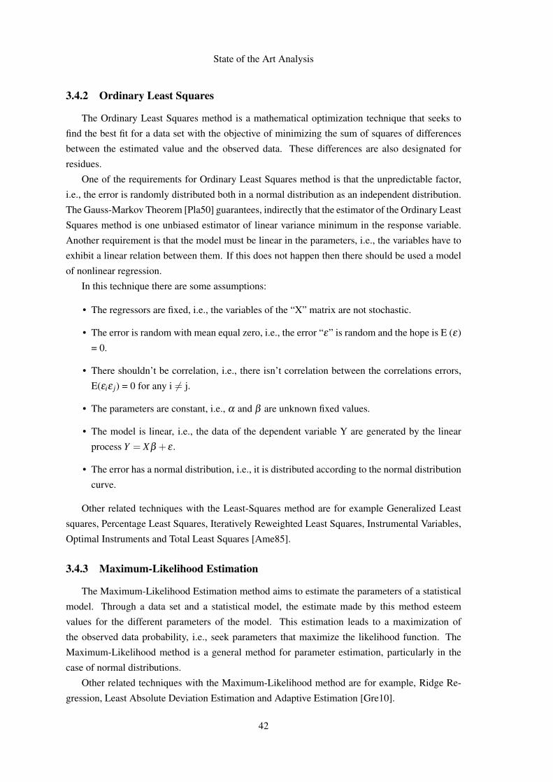
State of the Art Analysis
3.4.2 Ordinary Least Squares
The Ordinary Least Squares method is a mathematical optimization technique that seeks to
find the best fit for a data set with the objective of minimizing the sum of squares of differences
between the estimated value and the observed data. These differences are also designated for
residues.
One of the requirements for Ordinary Least Squares method is that the unpredictable factor,
i.e., the error is randomly distributed both in a normal distribution as an independent distribution.
The Gauss-Markov Theorem [Pla50] guarantees, indirectly that the estimator of the Ordinary Least
Squares method is one unbiased estimator of linear variance minimum in the response variable.
Another requirement is that the model must be linear in the parameters, i.e., the variables have to
exhibit a linear relation between them. If this does not happen then there should be used a model
of nonlinear regression.
In this technique there are some assumptions:
• The regressors are fixed, i.e., the variables of the “X” matrix are not stochastic.
• The error is random with mean equal zero, i.e., the error “ε” is random and the hope is E (ε)
= 0.
• There shouldn’t be correlation, i.e., there isn’t correlation between the correlations errors,
E(εiε j) = 0 for any i 6= j.
• The parameters are constant, i.e., α and β are unknown fixed values.
• The model is linear, i.e., the data of the dependent variable Y are generated by the linear
process Y = Xβ + ε .
• The error has a normal distribution, i.e., it is distributed according to the normal distribution
curve.
Other related techniques with the Least-Squares method are for example Generalized Least
squares, Percentage Least Squares, Iteratively Reweighted Least Squares, Instrumental Variables,
Optimal Instruments and Total Least Squares [Ame85].
3.4.3 Maximum-Likelihood Estimation
The Maximum-Likelihood Estimation method aims to estimate the parameters of a statistical
model. Through a data set and a statistical model, the estimate made by this method esteem
values for the different parameters of the model. This estimation leads to a maximization of
the observed data probability, i.e., seek parameters that maximize the likelihood function. The
Maximum-Likelihood method is a general method for parameter estimation, particularly in the
case of normal distributions.
Other related techniques with the Maximum-Likelihood method are for example, Ridge Re-
gression, Least Absolute Deviation Estimation and Adaptive Estimation [Gre10].
42
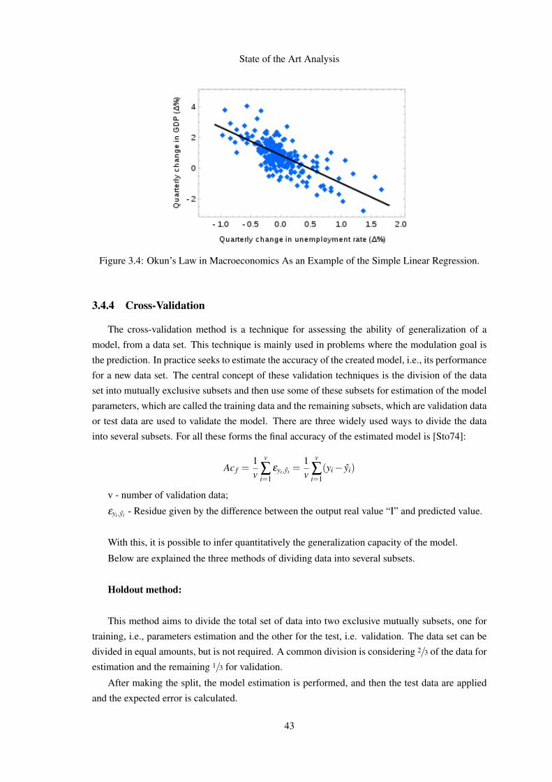
State of the Art Analysis
Figure 3.4: Okun’s Law in Macroeconomics As an Example of the Simple Linear Regression.
3.4.4 Cross-Validation
The cross-validation method is a technique for assessing the ability of generalization of a
model, from a data set. This technique is mainly used in problems where the modulation goal is
the prediction. In practice seeks to estimate the accuracy of the created model, i.e., its performance
for a new data set. The central concept of these validation techniques is the division of the data
set into mutually exclusive subsets and then use some of these subsets for estimation of the model
parameters, which are called the training data and the remaining subsets, which are validation data
or test data are used to validate the model. There are three widely used ways to divide the data
into several subsets. For all these forms the final accuracy of the estimated model is [Sto74]:
Ac f =1v
v
∑i=1
εyi,yi =1v
v
∑i=1
(yi− yi)
v - number of validation data;
εyi,yi - Residue given by the difference between the output real value “I” and predicted value.
With this, it is possible to infer quantitatively the generalization capacity of the model.
Below are explained the three methods of dividing data into several subsets.
Holdout method:
This method aims to divide the total set of data into two exclusive mutually subsets, one for
training, i.e., parameters estimation and the other for the test, i.e. validation. The data set can be
divided in equal amounts, but is not required. A common division is considering 2/3 of the data for
estimation and the remaining 1/3 for validation.
After making the split, the model estimation is performed, and then the test data are applied
and the expected error is calculated.
43

State of the Art Analysis
This approach is more suitable when a large amount of data is available. If the total data set is
small, the expected error can suffer a lot of variation [Koh95].
K-fold method:
The cross-validation method called K-fold, consists in dividing the total data set in "k" mu-
tually exclusive subsets with the same size, and from this, a subset is used for testing and the
remaining k-1 are used for estimation and consequently it is calculated the model accuracy. This
process is performed "k" times switching in a circular manner.
At the end of the "k" iterations it is calculated the accuracy on the found errors by the above
equation. Thus it is possible to obtain a measure with a higher degree of confidence about the
ability of the model to represent the data generating process [Koh95].
Method Leave-one-out:
The Leave-one-out method is a specific case of k-fold, with "k" equal to the total number of
data "N". In this approach are performed "N" error calculations, one for each data.
Despite a thorough investigation into the model variation in relation to the data used, this
method has a high computational cost, it is suitable for situations where little data are available
[Koh95].
3.4.5 Monte Carlo Method
The Monte Carlo method is any method of a class of statistical methods that are based on
massive random samples to obtain numerical results, i.e., repeating successive simulations a lot of
time. These kind of methods have been used for some time in order to obtain numerical approxi-
mations of complex functions where probably is impossible, to obtain an analytical solution, or at
least deterministic.
There are three classes of the Monte Carlo algorithms:
Unilateral Error Monte Carlo:
P - problem ;
A - random algorithm.
So "A" is a Unilateral Error Monte Carlo algorithm that solves "P" if the following require-
ments are met:
• For all configuration "x" that is not a solution of "P", prob (A ( x = YES ) ) ≥ 1/2.
• For all configuration "x" that is not a solution of "P", prob (A ( x = NO ) ) = 1.
44

State of the Art Analysis
In conclusion, whenever the answer is NO, the algorithm ensures the response certainty. How-
ever, if the answer is YES, the algorithm doesn’t guarantee that the answer is correct [Hro04].
Bilateral Error Monte Carlo:
A random algorithm "A" is a Bilateral Error Monte Carlo algorithm which assesses the "F"
problem if there is a positive real number “ε”, such that for all instance of "x" of the "F" [Hro04]:
prob (A (x) = F (x) ) ≥ 1/2 + ε
Not-Limited Error Monte Carlo:
The Not-Limited Monte Carlo algorithms are usually called Monte Carlo algorithms. A ran-
dom algorithm "A" is a Monte Carlo algorithm if for any input "x" of the “F” problem [Hro04]:
prob (A (x) = F (x) ) > 1/2
In addition to the mentioned algorithms there is another algorithm called Metropolis algo-
rithm which is probably the most Monte Carlo method used in Physics and aims to determine the
expected values of the simulated system properties by average over a sample.
The algorithm is designed to obtain a sample that follows a Boltzmann distribution.
The efficiency of the Metropolis algorithm is directly linked to the failure to take into account
the settings probability itself, but the ratio between them, since the ratio between the probabilities
of two settings that are given, can be determined independently of the others [MRR+53].
In Figure 3.5 is possible to see one example of the Monte Carlo Method application.
Figure 3.5: Monte Carlo Method Application to Determine the Lake Area.
3.4.6 Bootstrapping
The bootstrapping method is a resampling method which is used to approximate the distribu-
tion on a sample of a statistical survey data set, as well as to build confidence intervals or perform
45

State of the Art Analysis
hypotheses contrasts about interest parameters. In most cases it is not possible to obtain closed
expressions for the bootstrap approximations and thus it is necessary to obtain a resampling to im-
plement the method . The enormous calculation capacity of the actual computers greatly facilitates
the application of this method that is computationally very expensive.
The great advantage of this method is its simplicity. It’s a simple way to obtain estimates
of standard errors and confidence intervals for complex estimators of complex parameters of the
distribution, as percentile points, proportions, odds ratio, and correlation coefficients. Bootstrap is
also an appropriate way to control and verify the results stability. Although for some problems it
is impossible to know the true confidence interval, bootstrap is asymptotically more accurate than
the normal ranges obtained with variance and normality assumptions of the sample.
However this method also has its negative points. Although under certain conditions boot-
strapping is asymptotically consistent, it does not provide general finite guarantees of the sample.
The apparent simplicity can hide the fact that important assumptions are being made during the
bootstrap analysis, such as the independence of the samples where these would be most suitable
in other approaches [DE83].
In Figure 3.6 is possible to see the Bootstrap and Smooth Bootstrap Distributions.
Figure 3.6: Bootstrap and Smooth Bootstrap Distributions.
3.5 Conclusions
Through estimation methods it is possible to achieve a result with a much higher accuracy
when they are used by organizations to estimate their software development projects. The goal is
to use them individually or together, to obtain the best results, however, due to the limited time
available to complete this dissertation, sometimes it becomes impractical to study in greater detail
each of the methods.
46

State of the Art Analysis
In order to produce quality results, the estimation model to create needs templates with effort
costs per task in each estimation condition. Analyzing the described methods earlier, some of
them may lead to better results according to the projects to develop. According to the context and
company’s needs, probably the techniques of Individual Expert Judgment (see section 3.3.1) and
Wideband Delphi (see section 3.3.4). These techniques should be combined with model based
estimation techniques (e.g., COCOMO and PROBE) that are calibrated based on historical data,
using methods as the ones described in section 3.4.
47

State of the Art Analysis
48

Chapter 4
Model Proposal for Effort Distributionper Phase
In this chapter it is performed an analysis of the objectives of the creation of the estimation
model, analyzing the historical data provided by Altran, that will be crucial to work with the pre-
viously mentioned techniques in order to contribute for some improvements of the future projects
estimation of this company. Moreover, an effort analysis per phase of each project will be taken
and will be described the steps for the estimation model construction. Nearly the end will be ex-
plained the validation of this model and the impact that the variable "Duration" could have, if it
was included in the data analysis, aiming to achieve in the future a more complex and realistic
model.
4.1 Introduction
The proposal of the estimation model emerged with the Altran need to improve estimates of
their projects, including various technological options and thus support the teams that are dedi-
cated to the proposals elaboration for correctly estimate the effort of each project.
The creation of techniques to improve the models currently created by Altran, are more than
tools to improve effort estimates for projects to developed by this company. Through them, used
individually or even together can be minimized as much as possible the estimation error and thus
make the projects to develop more realistic and with higher quality. The idea of estimating the
effort of the projects per phase leads to greater monitoring of the projects, so not too much time is
available in the early phases and then the last phases being left with very little time to complete.
After being implemented these techniques for model creation, validation should be made using
some known techniques that make the model more realistic and not so skewed, and a validation
should also be taken by some experts of the company in order to verify whether the created model
49
Model Proposal for Effort Distribution per Phase
leads to possible improvements that through the models already created would not be possible to
achieve.
In these areas, such as science and technology, the uncertainty degree is usually so great that
exact and always correct estimates are impossible, and then a high error degree is expected and
should be accounted.
Thereafter it will be shown the proposed estimation methodology. This will focus on the
points where this dissertation will have more impact, in order to understand what really exists and
what can actually be changed or added so that in the future Altran can considerably improve their
estimates. In Figure 4.1, it is possible to observe the methodology followed, resembling a cycle
whose starting point is the Planning, specifically the Pre-Sale of a project. This methodology is
applied to various types of Altran projects. Before the projects enter in the Pre-Sale are initially
collected some important parameters to determinate the project complexity, as well as the customer
type and also the project size, for example. These parameters will influence the effort calculation.
Focusing more on this process, which begins with the Pre-Sale, it is noted that this step aims
to describe all the project requirements that will be evaluated. If the latter are approved, it is up
to the After-Sale personnel, who corresponds to the second step of this process, analyze again
the estimates that were made in the Pre-Sale and re-plan the project so that the project to develop
complies with the client requirements, so that he is satisfied with the project developed. Then,
the third step is the execution, where there is a percentage for the deviations, which correspond
to the associated risk with each project regarding the estimation that was taken previously. The
fourth step is to examine, analyze and give feedback about the estimates made and finally in the
last phase the Altran templates are used for each type of project to be developed in order to be able
to reach a satisfactory result.
This methodology is interesting, however, may not be the most accurate, and since the de-
viations are assigned may restrict somewhat the fact that the estimates were calculated for each
project. As such, there is the possibility of moving some metrics during the execution and also to
be able to change or improve some of the templates that currently Altran has for certain project
types, in order to obtain more consistent results. But the point where this dissertation will focus on
will be between the execution phase and the analysis and feedback phase, where a more detailed
analysis and feedback process will be taken. That is, according to historical data provided by
Altran, should be defined and applied feedback mechanisms with adjustable coefficients, before
using the templates for each type of project. Through historical data and techniques that were
already described, it is possible to apply cycle mechanisms on the sample so that the model will
be more reliable.
50

Model Proposal for Effort Distribution per Phase
Figure 4.1: Proposed Estimation Methodology.
4.2 Available Historical Data
This dissertation have a clear direction and meet the Altran needs, would need to be in posses-
sion the historical data from some past projects undertaken by this company. They were carefully
analyzed in order to see where there were gaps and where it is possible to improve so that future
projects have even more quality. The data availability provided by the company, is beyond doubt
one of the most important requirements of this dissertation.
As expected, the company doesn’t have to provide all the data of all projects that developed,
but a significant sample for analysis and the respective validation as realistic as possible. The
experience conducted in the future can then be put in competition with other projects in order to
verify whether it is effective, applied to any type of project.
In order to obtain a reasonable sample, was asked to Altran to make available historical data
from twenty-five past projects [Ann14]. The idea would then pick up on twenty such twenty-five
for estimation, and the remaining five projects would be to validate the model. Then, change the
projects in order to validate the model and make it less skewed and less biased.
Due to some unforeseen events, Altran could only make available historical data from six
projects. Although to be slightly lower than what was expected, there is sufficient data so that can
make an analysis of the sample and at the end using methods such as the Cross-Validation method
(see section 3.4.4), validate the respective model. In future if this work to reaches good results can
also apply these strategies to other projects with a larger sample, with more time, since the time
available for this dissertation is limited.
51

Model Proposal for Effort Distribution per Phase
The Table 4.1 shows the historical data in (man*day) provided by Altran.
Table 4.1: Historical Data Provided by Altran.
As shown in the table above, some projects don’t have separate data for the Development and
Tests phases. In order to make it more consistent, where all projects have the same phases, the
data was normalized by aggregating the Development ans Tests phases for all projects as shown
in Table 4.2:
Table 4.2: Historical Data Provided by Altran After Normalization.
As can be seen from Table 4.2 there are six projects, each one with a start date and an end date.
Each project has five phases [Kay14]:
• Analysis:In this first phase is made a systematic examination and the information or data are evaluated
and therefore the project is divided into several parts in order to verify the interrelationships
of the same. Here are also the requirements raised by the customer and the costumer needs
in the project realization. It’s also taken a specification aims precisely describe the tech-
nologies that will be used in the project implementation.
• Design:The Design phase is the second step in the project lifecycle. In this stage is taken a survey
of the technical requirements and is also taken a survey of the requirements of the reliability
testing. In this stage also, it is described the system architecture to be developed that will
be an abstract representation of the same. This architecture, ensures that the system to be
developed meet the project requirements and also ensure that future requirements can be
added.
52

Model Proposal for Effort Distribution per Phase
• Development and Tests:The third project phase corresponds to the Development project and Test project that aims to
check the proper functioning of the project. To summarize this phase serves to describe what
is necessary to develop the project in accordance with the Analysis and Design phases. The
main objective of Tests phase is to validate the developed project, testing each functionality
of each module, taking into account the details provided in the project first phase. Through
Tests phase could understand the project behavior, to correct some bugs that may arise.
• User Acceptance Testing:Almost at the end, the fourth phase corresponds to the User Acceptance Testing. In this
stage is made a test of Black-box testing to the project before it is made available to the
customer. The goal is to verify that the system meets the requirements established initially
and also the current user needs. Normally these tests are made by a small group of end users
in a similar environment with their environment. Criticisms and corrections will be posted
prior to delivering the project so that the project has a very similar to the expected behavior,
thus minimizing the number of bugs that may appear. Normally the project version at this
stage is called beta testing.
• Go-live:The Go-live phase is the last phase of the project and that the phase which apparently re-
quires less effort. This phase is important because it made the project closing and the last it
is to receive feedback from end users. It also made the system performance monitoring and
when necessary are made some minor adjustments to it. Ideas registration is done for future
design optimization at this phase and are also generated final reports of project management.
Moreover it is also analyzed the project team performance and is given the appropriate feed-
back. To finish, in this phase is also performed keeping the project developed over a number
of days to deal with the client.
The importance of each phase varies from project to project hence the effort to be different.
There are more complex projects than others and in these situations, certain phases will have a
different impact according to the importance they have in the project to develop.
As it is possible to see in all the projects, the data are divided into two parts. One for planned
data (Base) and another for the actual data. Although the planned data are important in the model
creation and as such will be taken into account in the calculations that will be made later, but what
interests analyzing is the actual data.
4.3 Initial Analysis
In this section, will be analyzed the historical data provided by Altran.
As can be seen, according to the data of each phase, was planned that GCU01 project is the
project with less effort. Through the actual data it was also demonstrated. The same happened to
the SRE02 project, but in this case the project which required greater effort.
53

Model Proposal for Effort Distribution per Phase
Looking again at Table 4.1 it can be seen that the Development + Tests phase, has a weight
of approximately 50% in each project. This makes sense, since it is the phase that requires more
effort in most projects of software engineering. It is also observed that the UAT phase, in the
last three projects varies greatly from what is expected to what really happened and certainly will
affect the final project estimation. The Go-live phase is the phase that requires less effort on all
projects and remains consistent in almost all projects. Analysis phase remains consistent in almost
all projects, except for SRE03 project, which is the only one where the predicted data are not
exactly like the actual data and which found a wide variation at this phase in relation to what
was expected. Contrary to the Design phase remains just the same with regard to planned and
what actually happened in GCU03 project. Overall, it is concluded that in the SRE01, SRE02 and
SRE03 projects, there is a greater variation in the data provided in relation to actual data which
may probably be the result of some problem related to the time management devoted to each
phase, since the difference between some phases is very considerable.
The effort of each phase of each project was divided by the total effort of the respective project.
Looking at Table 4.4 which corresponds to the actual data, it appears that the project that had least
value of percentage for effort in the Analysis phase was GCU02 project. The same happens for
GCU03 project, but in this case in the Design phase. Development + Tests phase remains more or
less constant hanging around 50%, which is normal. In UAT phase, the SRE01 project register the
slightest effort. The Go-live phase also maintains uniform in almost all projects.
After checking the facts stated, some assumptions must be made. Probably in the GCU02
project should be giving more attention to the Analysis phase, as well as in GCU03 project should
be giving more attention to the Design phase. Can also be seen as already mentioned in that
particular SRE01, SRE02 and SRE03 projects the predicted data is slightly different from the
actual data.
Table 4.3: Predicted Effort Percentage Per Phase.
54

Model Proposal for Effort Distribution per Phase
Table 4.4: Actual Effort Percentage Per Phase.
Thereafter is calculated, the Mean, Standard Deviation, and Quartiles, Upper and Lower, all
in percentage. Thus it is possible to know the average value per phase and the upper and lower
deviations from this value, for all available projects. This analysis will be done to the predictable
data as to the actual data either. In Tables 4.5 and 4.6 it is possible to view these data that was
calculated using spreadsheets.
Table 4.5: Statistics About the Predicted Effort Percentage Per Phase.
55
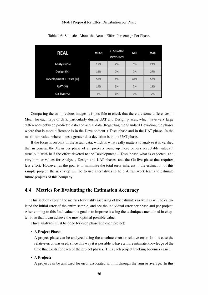
Model Proposal for Effort Distribution per Phase
Table 4.6: Statistics About the Actual Effort Percentage Per Phase.
Comparing the two previous images it is possible to check that there are some differences in
Mean for each type of data, particularly during UAT and Design phases, which have very large
differences between predicted data and actual data. Regarding the Standard Deviation, the phases
where that is more difference is in the Development + Tests phase and in the UAT phase. In the
maximum value, where notes a greater data deviation is in the UAT phase.
If the focus is on only in the actual data, which is what really matters to analyze it is verified
that in general the Mean per phase of all projects round up more or less acceptable values it
turns out, with half the effort devoted to the Development + Tests phase what is expected, and
very similar values for Analysis, Design and UAT phases, and the Go-live phase that requires
less effort. However, as the goal is to minimize the total error inherent in the estimation of this
sample project, the next step will be to use alternatives to help Altran work teams to estimate
future projects of this company.
4.4 Metrics for Evaluating the Estimation Accuracy
This section explain the metrics for quality assessing of the estimates as well as will be calcu-
lated the initial error of the entire sample, and see the individual error per phase and per project.
After coming to this final value, the goal is to improve it using the techniques mentioned in chap-
ter 3, so that it can achieve the most optimal possible value.
Three analyzes must be done for each phase and each project:
• A Project Phase:A project phase can be analyzed using the absolute error or relative error. In this case the
relative error was used, since this way it is possible to have a more intimate knowledge of the
time that exists for each of the project phases. Thus each project tracking becomes easier.
• A Project:A project can be analyzed for error associated with it, through the sum or average. In this
56

Model Proposal for Effort Distribution per Phase
case the average was used because it is more consistent and makes more sense than adding
all the errors associated to the project.
• A Set of Projects:For a set of projects, will also be used average instead sum for the same reasons stated in
the preceding paragraph.
In Table 4.7 it is possible to observe the initial errors for each phase and project.
Table 4.7: Initial Estimation Error of Each Phase in Each Project and Sample Total Error.
As can be seen in SRE03 project, specifically in the Go-live phase, the error was 118%, which
is huge. This error will have great weight in the average of the sample total error. The same
happens with the UAT and Design phases in SRE01 project. The phase where there was a minor
error of the sample, was the Development + Tests phase and the phase where there was a greater
error was in the UAT phase. Regarding projects, the project that contributes with less error for the
final score of the sample error was GCU03 project and the project that contributes with more error
was SRE01 project.
Each error of each phase was calculated using the following formula:
|ActualValue−PlannedValue |(ActualValue+PlannedValue
2 )
But what matters is actually knowing what was the total error of the available sample. So after
calculated all errors of all projects and phases as can be seen in Table 4.7, the next step was make
the average of all present errors and reached a final result as it possible to see in red. As it is
possible to see from the table above, the total error is very large, and it is necessary to minimize
it so that the projects are estimated in a more coherent way. The error module was used since
it allows aggregation. The relative error was used, since sometimes the absolute error isn’t very
significant.
The next section will show the proposed model to achieve less than the result obtained in
Table 4.7.
57

Model Proposal for Effort Distribution per Phase
4.5 Proposed Models for Estimation of the Phase Distribution
In order to be able to minimize the obtained error some models were built. In this section are
explained each of the two models that were conceived to improve the estimates situation of Altran.
Before explaining the calculation of each of the models listed hereafter in Figure 4.2, is illus-
trated how was processed the mechanisms of these models.
Figure 4.2: Process Mechanism of the Models.
The previous Process is illustrated in the following Figure 4.3 through an activity diagram:
58

Model Proposal for Effort Distribution per Phase
Figure 4.3: Activity Diagram of Process Mechanism of the Models.
4.5.1 Single-Value Model
In this model the predicted value for the effort percentage per phase for future projects is
simply the average from the past projects. Then applying the same formula set out in section 4.4
calculate the total error for all projects in order to verify if there were improvements in the error
obtained in Table 4.7.
In the Table 4.8 is possible to see the Single-Value Estimation Model.
59

Model Proposal for Effort Distribution per Phase
Table 4.8: Single-Value Estimation Model Calibrated Based on the Available Historical Data.
The calculation of this model consists; basically do the average of the available historical data.
Looking at Table 4.4 it was described previously, now have to make the average of each phase of
the entire sample.
Table 4.9 shows the estimation errors resulting from applying the model of Table 4.8 for the
projects GCU01 through SRE03. The average estimation is 27%. Although this table cannot be
used to validate the model, because the same data set is used to calibrate and apply the model, it
serves to set a limit on the estimation accuracy that could be achieved with this type of model.
Table 4.9: Single-Value Model Total Error.
4.5.2 Multi-Value Model
Given the significant variance found in the historical data, it was decided to propose another
model in order to further minimize the obtained error. For applying this model, we will require
that the user first estimates in T-shirt sizes (e.g., low, medium or high) the complexity of each
project phase. Then, the model will provide an estimate for the effort percentage depending on the
complexity level and historical data.
In the Table 4.10 it is possible to see the Multi-Value Model.
60

Model Proposal for Effort Distribution per Phase
Table 4.10: Multi-Value Estimation Model with T-Shirt Sizes.
This model consists in to creating a table with the same dimensions as Table 4.4 and along
with this to sort each percentage of each phase of each project, such as low, medium or high, so as
to group this set of percentages. In this way it is possible to know in which phases of each project
that had a minimum effort, which had an average effort and the ones with maximum effort. After,
the calibration factors should be used for the minimum and maximum values in order to optimize
the final error. The complexity table and the calibration factors can be seen in Table 4.11.
Table 4.11: Model Calibration.
The above table as analyzed and it is possible to see that each phase of each project has a
estimation classification. The UAT phase for example only has an average value but for example
the design phase has four average values. The scalars values can be set to be as beneficial to
minimize the total error. According to previous table, the best calibration factor is 1,25 for both
the lower and upper. To minimize the error, the model should allow choosing automatically the
complexity levels and k1 and k2 values.
The next step is to analyze Table 4.4 with Table 4.11 in order to establish conditions between
the two tables, so that, a new table appears with information about new effort new estimation of
each phase of each project, using this new model.
In T-shirt sizes table, the estimation classification should be:
• Medium: basically here the estimates values are equal to the Mean value calculated in
Table 4.6.
61

Model Proposal for Effort Distribution per Phase
• Low: here is→Mean - k1 * σ and respective normalization to 100%.
• High: here is→Mean + k2 * σ and respective normalization to 100%.
Where:
k1, k2 are chosen to minimize the error.
It is noted that k1 and k2 correspond to –StndDev and +StndDev, respectively, according to
Table 4.11.
According to what has been said so at this time it is now possible to obtain a new estimation
of historical data available. In Table 4.12, it is possible to observe the new estimation:
Table 4.12: Multi-Value Estimation Model
As is easily seen, in the previous table, there is a small detail. The sum of the percentages of
all project phases doesn’t give 100%, that means to get the right values of the new estimation has
to adjust these percentages so that the total of all the phases of each project is 100%. To resolve
this, it is relatively easy. Simply just divide the value of each estimate of each phase of each
project by the total sum of the estimates obtained in that project. So the new table, with the data
normalization may be displayed by Table 4.13.
62

Model Proposal for Effort Distribution per Phase
Table 4.13: Multi-Value Estimation Model After Normalization.
Table 4.14 shows the estimation errors resulting from applying the model of Table 4.10 for the
projects GCU01 through SRE03. The average estimation error is 9%. Although this table cannot
be used to validate the model, because the same data set is used to calibrate and apply the model,
it serves to set a limit on the estimation accuracy that could be achieved with this type of model.
Table 4.14: Multi-Value Model Total Error.
How it is easy to understand, the Multi-Value model achieves a sample total error lower than
Single-Value Model. This model improve the initial estimate shown in Table 4.7.
Once constructed the two models, now it’s time to the validation step in order to prove its
effectiveness. In the following section will be displayed the chosen validation form.
4.6 Model Validation
In order to prove that the constructed model is really reliable and even improve Altran current
estimates, it is necessary to use validation techniques already mentioned previously in section 3.4
63

Model Proposal for Effort Distribution per Phase
It was decided to only validate the Single-Value Model relating on the available historical data
average. We choose not to perform a cross validation of the Multi-Value Model because of the
lack of sufficient historical data.
The method chosen to validate the Single-Value Model was the Cross-Validation method out-
lined in section 3.4.4 and then will be shown all the steps for validation.
Starting this process, it is necessary to rebuild the Table 4.6, but considering all projects except
the first, GCU01, since this process is in a cyclical process that aims to calculate the error of each
individual project and at the end is made the average for all projects.
Then to obtain the error of each phase of this project, should be put the column of Table 4.6
regarding this project and compare it with the Mean column of the Table 4.15. Thus, it is obtained
the errors of each phase of the GCU01 project, as shown in Table 4.15.
After calculated the errors for each project, the last step is to calculate the sample total error.
This representation can be seen from Table 4.15.
64

ModelProposalforE
ffortDistribution
perPhase
Table 4.15: Single-Value Model Total Error Using Cross-Validation.
As is to possible to see from the previous figure, using the validation technique, which makes the model chosen less biased and more reliable, the
total error obtained is less than the error that was initially obtained as seen in Table 4.7.
Although this validation reach a better result than the current, it is still necessary that some Altran experts validate the model in order to further
prove its reliability.
65

Model Proposal for Effort Distribution per Phase
4.7 Duration Impact
As it is possible to see from Table 4.1, it was available the start and end dates of each project.
Then, through those dates, it is possible to know the duration of each project. As can be seen in
Table 4.16, each project has duration in days:
Table 4.16: Historical Data Provided by Altran With Duration Variable.
Although this variable was not included in the projects estimation, it is important to refer to
the future, because it may influence the estimation of the projects to be developed by Altan.
Below in Table 4.17 is shown the correlation of the actual effort percentage of each phase.
Table 4.17: Correlation of Each Phase of Each Project with Duration Variable.
The correlation coefficient indicates the strength and direction of the linear relationship be-
tween two variables. The correlation fails to capture dependence in some instances. In general it
is possible to show that there are pairs of random variables with strong statistical dependence and
however have null correlation. For this case should be use other dependence measures.
Then are presented the formulas for calculating the correlation coefficient between two vari-
ables.
Pearson’s Product-Moment Coefficient:
66

Model Proposal for Effort Distribution per Phase
The correlation coefficient ρX ,Y between two random variables X and Y with expected values
µx and µy and standard deviations σx and σy is defined as [RN88]:
ρX ,Y =cov(X ,Y )
σxσy=
(E((X−µx)(Y −µy))
σxσy
where:
E: expected value operator.
cov: covariance.
As:
µx = E(X),σx2 = E(X2)−E2(X)
and similarly for Y, we can also write:
ρX ,Y =E(XY )−E(X)E(Y )
(√
E(X2)−E2(X))(√
E(Y 2)−E2(Y ))
The correlation is defined only if both the standard deviations are finite and not null. The
Cauchy- Schwarz corollary inequality [QS10], the correlation can not exceed 1 in absolute value.
According to what has been said has more sense grouping phases of the project into two parts
in order to stay with only two variables. So, Table 4.17 will stay this way, as can be seen from
Table 4.18.
Table 4.18: New Correlation Dividing the Project Into Two Parts with Duration Variable.
As it is possible to see from the above table, the two correlations are smaller than 1 in absolute
value and have opposite direction because they are symmetrical. Below in Figures 4.4 and 4.5 it
67

Model Proposal for Effort Distribution per Phase
is possible to see the correlation graphs between the duration variable with each of the two parts
of the project.
Figure 4.4: Correlation Between Analysis + Design Phases with Duration Variable.
Figure 4.5: Correlation Between the Other Phases with Duration Variable.
A possible way to take into account project duration is by building a linear regression model
(see section 3.4.1) for the effort percentage for each phase as a function of the project duration.
We don’t build such model because of the lack of sufficient historical data.
Another possibility would consist in discretizing the duration estimates by T-shirt sizes (e.g.,
low, medium or high).
68

Chapter 5
Conclusions and Future Work
In this section some conclusions will be taken and some future work will be suggested.
5.1 Conclusions
It can be concluded that this dissertation addresses of a different way the estimation process
followed by Altran Portugal.
In the first part of this dissertation, some estimation methods were analyzed and techniques,
which are the state of the art and allowed some improvements of the current method used by
Altran Portugal. The current situation of the company was analyzed, too, in order to understand
their needs.
The models provided by Altran, helped to understand some metrics that should be followed
and were important to understand which variables influenced the final calculation of the estimation
error associated with the available sample. It was concluded easily that the historical data regard-
ing to the past projects, that Altran released, was one of the main requirements of this dissertation,
since without them, this dissertation didn’t make much sense.
The model created had as goal use different estimation methods and techniques, along with
the CMMI processes and practices. It should be borne in mind that a model was built to ensure
that in future the management and evolution of that model is easily achieved. It was also expected
that the model created, improve productivity analysis, which so far is a bit limited, and also allow
a more simple and intuitive for those using it.
The main differences added, focused on individual estimation of the distribution per phases of
each project. This way will improve the productivity analysis, as well as allowing a simpler and
easier process estimate. It can be said that it is an innovative approach compared to the existing
one.
Due to limited time for conducting this dissertation, some tests are planned, beyond the scope
of this dissertation, which will aim to assess the reliability of the built model. Some usability tests
69

Conclusions and Future Work
should also be made to avoid certain bugs that may arise and some questionnaires so should also
be made that certain requirements are met, as they are essential for the proper functioning of the
built model.
Increasingly companies invest in these methodologies in order to be able to obtain a greater
long-term productivity and achieve better organize the estimates of their projects.
The proposal goals for this dissertation in general have been met, however, the ambition in
the initial phase, led to an even more comprehensive set of improvements. Anyway, the em-
ployees who followed this project agree that the results were successfully achieved and that the
constructed model is intuitive and satisfying their needs with regarding to the estimation of their
projects. Through what was described in this dissertation it is noted that the model that was val-
idated improve the initial error of the sample provided, approximately in 26%. The other model,
more complex, based on multi-values, wasn’t validated, and as such becomes a little biased state
its improves, however, achieved to values that improved the initial error in 79%.
In the future, after this model begins to be implemented at Altran, it is expected that their teams
are motivated to use this model in different project types, since it has simplified the estimation
process and improve the quality of its estimates.
These evolutions represent a major step in the estimation process and may represent a very
valuable contribution to Altran Portugal.
5.2 Future Work
Although the results have been successfully achieved, should be taken a more detailed anal-
ysis of the problems that may occur and evaluate a set of determinants criteria for the proper
functioning of this type of models.
This version added, is still very premature and new suggestions will be important to increase
the estimation quality through variables more targeted to the project type to implement. Some
tests should be made to validate the proposed model and thus it can be used in Altran upcoming
projects.
One of the improvements for this project may be adding more methods and estimation tech-
niques outlined in the state of the art, specifically in section 3.3.
Some PSP [Hum05] and TSP [Hum99] metrics can be used to study in more detail the pre-
dictability.
In future, there is a possibility to take into account the project type, i.e., different calibrations
for different project types. Furthermore, there is a possibility to have different calibrations factors
(K) per phases.
The expectations for the future is that Altran can successfully manage the available resources
in the company, along with the improvement of the estimation process of the projects to develop.
Finally, is concluded that one of the main threats of this dissertation is its management and the
time available for its completion. So that the goals are successfully achieved, is necessary to plan
and to structure the different work tasks sequentially. However during this first phase there was a
70

Conclusions and Future Work
big effort to get meet deadlines due to interest in work theme and the areas addressed in the same,
trying from start to meet the proposal goals, in order to successfully complete the realization of
this dissertation. At the moment, there is a great motivation to continue to develop this work after
the final delivery, because this work can be more complete and more complex, in order to be more
advantageous for this company.
71

Conclusions and Future Work
72

References
[Abr02] Pekka Abrahamsson. Agile Software Development Methods: Review and Analysis.VTT Technical Research Centre of Finland, 2002.
[Ame85] Takeshi Amemiya. Advanced Econometrics. Harvard University Press, 1st edition,November 1985.
[Ann14] Charles Annis. Central Limit Theorem. Accessed http://www.statisticalengineering.com/central_limit_theorem.htm, Jan-uary 2014.
[Boe81] Barry W. Boehm. Software Engineering Economics. Prentice Hall, 1st edition,November 1981.
[CKS11] Mary Beth Chrissis, Mike Konrad, and Sandy Shrum. CMMI for Development, v1.3:Guidelines for Process Integration and Product Improvement. SEI Series in SoftwareEngineering. Addison-Wesley Professional, 3rd edition, March 2011.
[Coh05] Mike Cohn. Agile Estimating and Planning. Prentice Hall, 1st edition, November2005.
[DE83] Persi Diaconis and Bradley Efron. Computer-Intensive Methods in Statistics. Tech-nical Report 83, Division of Biostatistics, Stanford University, January 1983.
[Fun13] FunctionPoints.org. Function Points Analysis. Accessed http://www.functionpoints.org/function-point-analysis.html, July 2013.
[GGK06] Diane Gibson, Dennis Goldenson, and Keith Kost. Performance Results of CMMI-Based Process Improvement. Technical report, Software Engineering Institute, Au-gust 2006.
[God13] Sally Godfrey. What is CMMI. Accessed http://www.docstoc.com/docs/29849281/What-is-CMMI-%28PowerPoint%29, July 2013.
[Gre02] James W. Grenning. Planning Poker. Renaissance Software Consulting, April 2002.
[Gre10] William Greene. Maximum Simulated Likelihood Methods and Applications, vol-ume 26 of Advances in Econometrics. Emerald Group Publishing Limited, 1st edition,December 2010.
[Hel95] Roger Heller. An Introduction to Function Point Analysis. CrossTalk, The Journal ofDefense Software Engineering, 8(11):24–26, November/December 1995.
73

REFERENCES
[Hro04] Juraj Hromkovic. Algorithmics for Hard Problems: Introduction to CombinatorialOptimization, Randomization, Approximation, and Heuristics. Springer, 2nd edition,April 2004.
[Hum99] Watts S. Humphrey. Introduction to the Team Software Process. Addison-WesleyProfessional, 1st edition, September 1999.
[Hum05] Watts S. Humphrey. PSP(sm): A Self-Improvement Process for Software Engineers.Addison-Wesley Professional, March 2005.
[Jon09] Capers Jones. Software Engineering Best Practices: Lessons from Successful Projectsin the Top Companies. McGraw-Hill Osborne Media, 1st edition, October 2009.
[Jør04a] Magne Jørgensen. A Review of Studies on Expert Estimation of Software Develop-ment Effort. Journal of Systems and Software, 70(1–2):37 – 60, February 2004.
[Jør04b] Magne Jørgensen. Top-down and Bottom-up Expert Estimation of Software Devel-opment Effort. Information and Software Technology, 46(1):3 – 16, January 2004.
[Kay14] Russell Kay. QuickStudy: System Development Life Cycle. Accessedhttp://www.computerworld.com/s/article/71151/System_Development_Life_Cycle, January 2014.
[Koh95] Ron Kohavi. A Study of Cross-Validation and Bootstrap for Accuracy Estima-tion and Model Selection. International Joint Conference on Artificial Intelligence,14(1):1137–1145, August 1995.
[McC06] Steve McConnell. Software Estimation: Demystifying the Black Art. Best Practices(Microsoft). Microsoft Press, March 2006.
[MGB74] Alexander M. Mood, Franklin A. Graybill, and Duane C. Boes. Introduction to theTheory of Statistics. McGraw Hill, 3rd edition, June 1974.
[MRR+53] Nicholas Metropolis, Arianna W. Rosenbluth, Marshall N. Rosenbluth, Augusta H.Teller, and Edward Teller. Equation of State Calculations by Fast Computing Ma-chines. Journal of Chemical Physics, 21(6):1087–1092, June 1953.
[Pla50] Robin L. Plackett. Some Theorems in Least Squares. Biometrika, 1950.
[Por13] Altran Portugal. Accessed http://www.altran.pt/sobre-nos/altran-portugal.html, July 2013.
[QS10] João Filipe Queiró and Ana Paula Santana. Introdução à Álgebra Linear. GradivaPublicações, 1st edition, 2010.
[Rei08] Elizabeth Reis. Estatística Descritiva. Edições Sílabo, 7th edition, 2008.
[RN88] Joseph Lee Rodgers and W. Alan Nicewander. Thirteen Ways to Look at the Correla-tion Coefficient. The American Statistician, 42(1):59–66, February 1988.
[Sch06] Rob Schoedel. PROxy Based Estimation (PROBE) for Structured Query Language(SQL). Technical report, Software Engineering Institute, May 2006.
[SG05] Andrew Stellman and Jennifer Greene. Applied Software Project Management.O’Reilly Media, Inc, 1st edition, November 2005.
74

REFERENCES
[Sri14] Vibhu Srinivasan. What is a Story Point? Accessed http://agilefaq.wordpress.com/2007/11/13/what-is-a-story-point/, February 2014.
[Sto74] M. Stone. Cross-Validatory Choice and Assessment of Statistical Predictions. Journalof the Royal Statistical Society. Series B (Methodological), 36(2):111–147, January1974.
[Tea10] CMMI Product Team. CMMI For Services, Version 1.3. Technical report, SoftwareEngineering Institute, November 2010.
[The92] Henri Theil. Henri Theil’s Contributions to Economics and Econometrics. SpringerNetherlands, 1992.
[Wei14] Jeremy Weiskotten. Velocity: Measuring and Planning an Agile Project.Accessed http://agilesoftwaredevelopment.com/blog/jeremy/velocity-measuring-and-planning-agil, February 2014.
75

REFERENCES
76
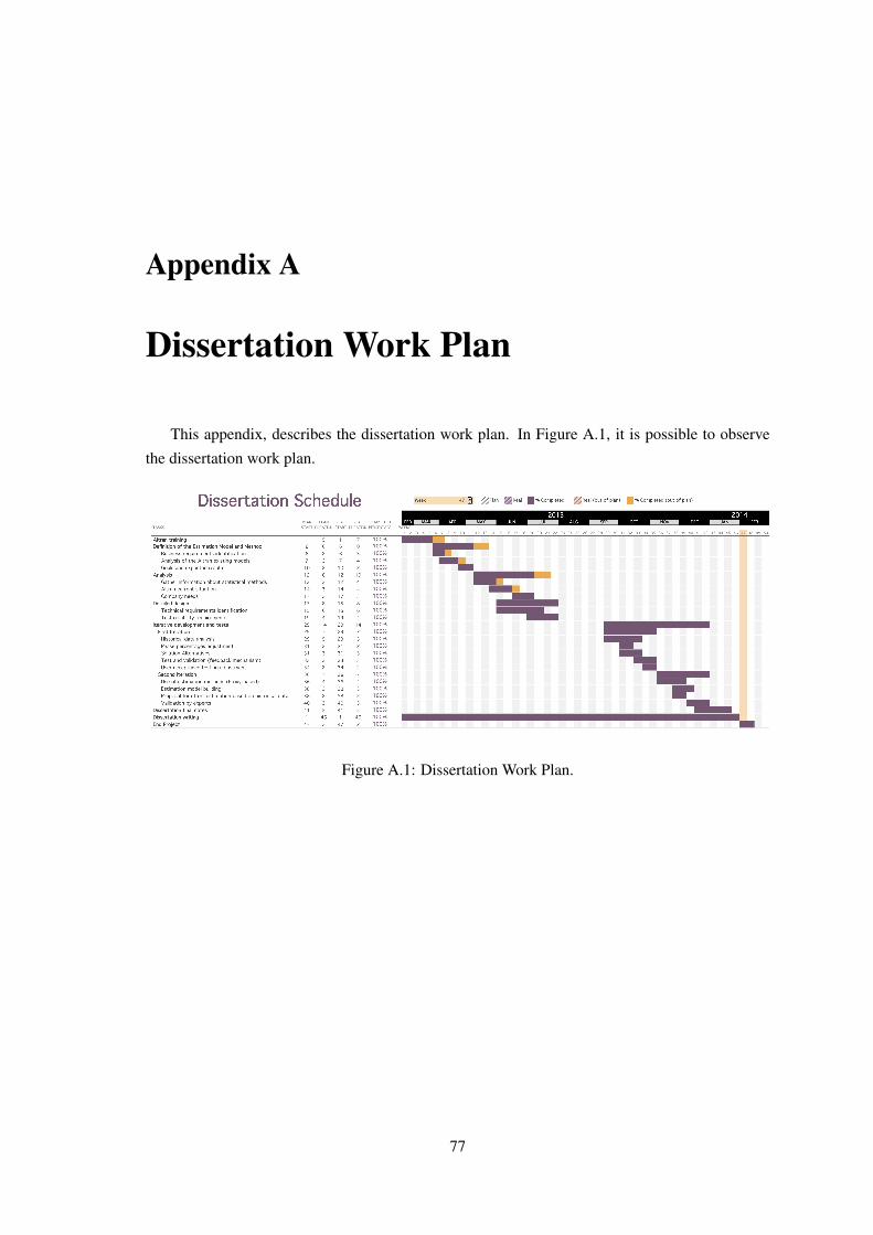
Appendix A
Dissertation Work Plan
This appendix, describes the dissertation work plan. In Figure A.1, it is possible to observe
the dissertation work plan.
Figure A.1: Dissertation Work Plan.
77

Dissertation Work Plan
78

Appendix B
Altran Estimation Templates
This appendix shows some figures that complement others that were shown previously regard-
ing of the estimation models that Altran has currently.
B.1 Altran Template for EDP Projects
This section will show the different parts that constitute the template for Altran projects of
EDP company, in order to understand in more detail the model building.
Figure B.1: Cover of EDP Template.
79

Altran
Estim
ationTem
plates
Figure B.2: Estimates of EDP Template.
80

Altran Estimation Templates
Figure B.3: Profiles of EDP Template.
B.2 Altran Template for Oracle Projects
This section will show the different parts that constitute the template of Altran for Oracle
projects, in order to understand in more details the model building.
Figure B.4: Cover of Oracle Template.
Figure B.5: Effort Sum of Oracle Template.
81

Altran
Estim
ationTem
plates
Figure B.6: Estimates of Oracle Template.
82

Altran Estimation Templates
Figure B.7: Value Adjustment Factor of Oracle Template.
Figure B.8: Guidelines of Oracle Template.
83

Altran
Estim
ationTem
plates
Figure B.9: Reference Data of Oracle Template.
84

Altran Estimation Templates
B.3 Altran Template of Data Extraction Estimates for Oracle-EBSProjects
This section will show the different parts that constitute the template of Altran for Oracle-EBS
projects, in order to understand in more detail the model building.
Figure B.10: Estimates of Oracle-EBS Template.
85

Altran
Estim
ationTem
plates
Figure B.11: Assumptions of Oracle-EBS Template.
86

Altran
Estim
ationTem
plates
B.4 Altran Template for Change Request Estimates
This section will show the different parts that constitute the template of Altran for change request projects, in order to understand in more detail the
model building.
Figure B.12: Estimates of Change Request Template.
87