Improving PH1120 Physics Labs

An Interactive Qualifying Project Report

Submitted to the Faculty of the

WORCESTER POLYTECHNIC INSTITUTE

in partial fulfillment of the requirements for the

Degree of Bachelor of Science

in Physics

By

Bryan Bergeron

Date: August 18, 2012

Advisor:

Prof. Germano S. Iannacchione

Department of Physics

Abstract

The physics labs for WPI's PH1120 course were updated in an effort to make them more

interactive, instructive, and easier to understand. One of the labs was redesigned from the ground

up, otherwise the original lab instructions were used as a starting point. Additionally most of the

lab report questions were rewritten in an effort to make them more relevant to the lab itself, and

to ensure that the students understand the science. Pictures of laboratory equipment and

apparatuses were included so that students know if their assembly is correct.

Acknowledgements

I would like to thank my advisor, Germano Iannacchione, for helping me to find a project

and for helping me to make an easy transition back into school. I would also like to thank lab

manager Fred Hutson, for all of his guidance and assistance.

Table of Contents

Abstract ......................................................................................................................................... 2

Acknowledgements ...................................................................................................................... 3

Project summary .......................................................................................................................... 5

Lab instructions ........................................................................................................................... 8

Lab 1 .................................................................................................................................. 8

Lab 2 .................................................................................................................................. 9

Lab 3 ................................................................................................................................ 12

Lab 4 ................................................................................................................................ 16

Lab 5 ................................................................................................................................ 21

Lab 6 ................................................................................................................................ 27

Lab 7 ................................................................................................................................ 34

Lab 8 ................................................................................................................................ 37

Lab reports ................................................................................................................................. 42

Lab 1 ................................................................................................................................ 42

Lab 2 ................................................................................................................................ 43

Lab 3 ................................................................................................................................ 44

Lab 4 ................................................................................................................................ 46

Lab 5 ................................................................................................................................ 48

Lab 6 ................................................................................................................................ 49

Lab 7 ................................................................................................................................ 52

Lab 8 ................................................................................................................................ 53

Conclusion .................................................................................................................................. 54

Project Summary

In this project I reviewed the lab materials for the PH 1120 electricity and magnetism

class here at WPI, with the purpose of editing them, improving them, expanding upon them, and

in some cases remaking them, for the betterment of the students' learning experience. The

general topic of this project was suggested to me as part of a continual effort by the physics

department to improve all of its freshmen 1000 level sequence physics laboratory assignments;

the goal was to obtain an outsiders perspective of what could be improved. After reviewing some

of the materials I decided that a good area of focus for me would be the PH 1120 labs. I came to

the conclusion that the greatest need for change came from the difficulty a student may have in

understanding what is expected of them, and how what they are doing relates to what they are

learning in lectures, and the subject as a whole. By rewriting much of the lab instructions and

including pictures of what the labs are supposed to look like, I hoped to make them simpler for

the students to understand the process and easier for them to learn the material. I also tried to

improve how the student related what they are doing to the subject by changing or amending the

lab reports, forcing the students to think more critically about what they have done and what it

means. My efforts on this project should make the PH 1120 simpler for students follow and

increase their overall usefulness in improving the students' understanding of the material.

The goal of the physics department in establishing this IQP was to find ways that the

assignments can be improved upon by seeking a student's perspective. As someone who has

learned the material comparatively recently, a student is more likely to anticipate what may

cause new students difficulty; a student should have learned the material recently enough to

remember his own struggles and be able to relate to someone who doesn't know the material,

whereas a professor who has known everything for decades may not always see when something

is unclear. Also it is useful to have someone new look at the material with a fresh pair of eyes

simply for editing purposes. The objective given to me was to use my outside perspective to look

for problems the faculty may have overlooked and to contribute my own ideas to the ever

changing laboratory assignments.

After learning of the assignment I reviewed the laboratory assignments for the first two

classes in the freshmen physics sequence: 1110, and 1120. These two classes are considered

almost compulsory education at WPI, taken by the majority of freshman, often in their first term.

Also of note is that these are the less ambitious of two sets of classes covering the same material,

and are designed specifically for non-physics majors with no prior knowledge of the material.

Because of all this the majority of the students in these courses have no experience in physics

and likely no experience in a laboratory environment at all. Because of this it is more important

than is more advanced physics courses that the instructions given to students be as descriptive

and informative as possible. The laboratory assignments need to be completely up front about

what is expected of the students and need to get them accustomed to the laboratory experience,

as well as show them how to apply the experiments to what they are being taught in lectures.

After reviewing the laboratory assignments for both classes, I concluded that the

assignments for PH1120 were significantly less instructive and informative than those for

PH1110. The assignments for PH1110 gave very clear instructions, and supplied pictures of the

lab equipment and of what the apparatus should look like, provided clear instructions on how to

use them. The PH1120 assignments by comparison were significantly harder to follow so that the

student would sometimes think they were ambiguous, and they lacked pictures of properly set up

apparatuses that would allow students to check what they have done. I decided to dedicate the

bulk of my work on the project to making the instructions easier for the students to understand. I

also found that for many of the labs, the lab report questions did not always properly engage the

student with studying the results of the experiment and understanding what those results mean. I

decided that many of these problems could be improved by rewriting instructions for each of the

labs with more instructive detail, providing pictures of the equipment and properly prepared

apparatuses, and to add or edit lab report questions so as to better promote the students'

knowledge and understanding of the concepts.

I began my work by attending a few of the lab sessions for the class that was being run

concurrently with my project. After observing the students work, and talking to some of them, as

well as others I knew who had completed the class recently, the biggest problem I learned of was

that none of the students were completing the actual experiment for the first two labs. The first

two labs do not require any work with actual equipment, so instead of coming to lab and going

through the experiment, they would simply skip to the lab report questions which could be

answered easily without having done the work. Lab 2, which tasked students with drawing

electric field lines, was especially avoided. The experiment required students to manually draw

in the electric field lines for various configurations of point charges using Microsoft Paint. This

resulted in several problems. It was not sufficiently engaging, as it required to students to go

through the process of saving an image file of the worksheet to their PC so it can be opened in

MS Paint, and to go through an annoying process of struggling to draw decent lines using a

mouse, which does provide nearly the dexterity of an pen and paper. The process was far too

complicated and difficult, and did not provide much benefit to the student anyway. Also the lab

report questions could easily have been answered without having attended the lab. This all set a

bad precedent for future labs, because if students got used to the lab session not being necessary

in the early labs, they may be disinclined to show up or be prepared for later labs. My solution to

this was to redesign how the lab was performed. Rather than have students manually draw

electric field lines, I wrote a lab that would have them use a Java applet to help them visualize

what the lines should look like. The new lab would require students to set up the configurations

of charges in the applet and analyzing the results, thus being more interactive and thought

provoking than the original. Additionally some of the new lab report questions would refer

directly to work the students would had to have already completed in the lab session. The new

lab should better ensure that students will go through with the experiment, and better supplement

their understanding of the concept.

That was just one example of what I found needed to be done. Most of the other labs I

found to require far less comprehensive changes, although I made at least some adjustments to

all of them. Lab 1 for example, which had some of the same problems as lab 2, I concluded could

be fixed by simply making the lab report more thought provoking so as to require students to

think about the work that they did, and also by more explicitly telling students in the instructions

what they were expected to do. Labs 7 and 8 by comparison, I found to be quite well designed

already; the only improvements I could think to make were to edit the instructions for grammar

and clarity, and to rewrite some of the lab report questions to be more thought provoking. For

each of the 8 labs I went through looking for things that were unclear, things that a student might

do incorrectly, and things where the student might not see the significance of why he was doing

it and sought to improve them by rewriting parts of the lab instructions and changing many of the

lab report questions.

Probably the most basic, but arguably the most significant improvements I made to each

of the labs was to include pictures of the apparatus, and to provide a somewhat more consistent

format for the lab instructions. The pictures should help the students to see how everything is

supposed to look when set up correctly, which should cut down on their confusion, limit the

number of questions being asked of the TA's and make the lab time more productive. If a student

is confused about whether they did something correctly, rather than waffling around deciding

whether to ask for help and trying to peak at what everyone else is doing, they can simply refer

to the picture. It will also allow more diligent students to look at the pictures beforehand so they

have an idea of what they will be dealing with before they come to class. I also rewrote many of

the introductions with an eye toward helping to prepare students reading them before class. Also

as previously mentioned I attempted to implement a consistent format for how the instructions

were written. By getting the student used to an order of introduction, purpose, set-up, procedure,

and calculations, they would be more used to what they would be likely to see in labs for more

advanced classes.

The Electric Field

Purpose

To acquaint you with the properties and behavior of the electric fields and to get you accustomed to

what is expected of you in future labs.

For each lab the lab instructions will contain links to a lab data sheet and a lab report. The data sheet is

filled out during the experiment and submitted online at the end of the period. The data sheet is not

graded, but is evidence of you work in the lab; it is also important for practicing the techniques in the lab

and will often be useful for collecting data to be used when completing the lab report. The lab report is

what is actually graded, and consists of questions designed to test your knowledge of the concepts

covered in the lab and may include short-answer questions, calculations based on the processing of raw

data, and critical thinking. Lab reports are to be submitted online by midnight of the day the lab takes

place, and you may begin working on them as soon as the experiment is finished and your data sheet is

submitted online.

Procedure

The electric field is a vector quantity whose magnitude and direction are equal to that of the force felt

by a positive test charge of 1 coulomb placed at the point in question. In this experiment you will be

analyzing the electric field produced by point charges and drawing arrows representing the electric field

vector; the length of which is proportional to the strength of the electric field, and the direction of which

is equivalent to that of the electric field. As a basis for the scale for this lab, a charge of 1 coulomb 1 unit

away from the indicated point should result in an arrow of length 1 unit.

There are THREE parameters to keep in mind in figuring out the strength and direction of the electric

field at a point due to a nearby electric point charge – the POLARITY of the charge (positive or negative),

the MAGNITUDE ׀q׀ of the charge, and the DISTANCE r between the point-charge location and the point

where the electric field is being evaluated. The strength of the electric field at that point of evaluation is

directly proportional to ׀q׀ and inversely proportional to r2. The electric field direction points directly

away from a positive point charge and directed toward a negative point charge. In a situation involving

two or more point charges, the analysis simply involves the linear superposition of the individual effects

of each point charge separately, and that’s a REALLY important aspect of this laboratory exercise.

On the data sheet you are to draw in the arrows for the electric field at the designated point and fill in

the values for the missing quantities. L and Ɵ are the polar coordinates for the arrow and n is the charge

of the point charge.

Electric Fields & Field Lines

pre-lab

The purpose of this experiment is to acquaint you with electric field lines. Remember electric field lines

are lines that trace the direction of the electric field until they terminate at either infinity, or a negative

charge. Before coming to lab, follow the link to a java applet on electric field lines, and take a few

minutes to play around with it to get a feel for how field lines work.

http://www.falstad.com/emstatic/index.html

When the Java window opens up, uncheck the option 'Draw Equipotentials', and on the third

dropdown box select 'Show E lines'. At this point you should have a single positive charge with electric

field lines going away from it in all directions. You can add additional point charges by going to the

'Mouse =' dropdown box and selecting positive or negative draggable charges, and then clicking

anywhere on the display. Experiment with different numbers of charges and moving them around in

different orientations to see how the field lines are affected. Also experiment with adding conductors by

going to the 'Mouse =' dropdown box again and selecting 'Add Conductor (Gnd)'. You can then draw in

conductors by holding down the left mouse button and dragging the cursor. This is also a useful applet

for visualizing field vectors and equipotential lines, but that is not the topic of this lab. As you are going

through lab, try to guess what the field lines will look like before you set up each situation, and explain

to yourself afterward why it looks the way it does.

Purpose

The goal of this lab is to get you to understand how electric field lines work and be able to

visualize what they should look like. You should also have a theoretical understanding of how to

interpret them and what they mean.

Set-up

By now hopefully you have had the opportunity to play around with the applet and have figured

out how it works, but I will explain everything in detail regardless. To start simply follow this link to the

applet and it will pop up. Our focus for this lab is on electric field lines, so deselect the 'Draw

Equipotentials' option, and under the 'Show' dropdown menu select 'Show E lines'. You may want to

adjust the resolution or brightness using the scroll bars however you like. It is important to note that the

brightness at any one point is an indicator of the strength of the electric field at that point, bright white

indicates a strong electric field, and dark green a weak field. You will be adding, deleting, and moving

around point charges as you go along, and to do so you access the 'Mouse =' dropdown box. It is fairly

self explanatory, this box changes what the mouse does. To add charges select 'Mouse = Add (+,-)

Draggable Charge' and click anywhere on the display. To move them around or delete them select 'move

object' or 'delete object' respectably. You can change the strength of a point charge by selecting 'Mouse

= Adjust Charge' and clicking on a point and dragging out a rectangle around the charge, then you can

adjust it using the charge scrollbar that appears. Keep in mind the default charge is ±1 and the scrollbar

allows values between ±2. To add a conductor, select 'Mouse = Add Conductor (Gnd)' and hold down

the left mouse button as you draw in the desired shape. If you screw up drawing a conductor you can

touch it up by selecting 'Mouse = Clear Square' and clicking on any one point to delete a small part of

the conductor.

Procedure

Create the following situations using the controls just described, and as you do so, make sure to

notice several things: How many field line from positive charges are terminating at infinity, conversely

how many starting at infinity are terminating at negative charges, also pay attention to where the

electric field is strongest and where it is weakest, indicated by the brightness of the field lines. Adjust

the brightness dial if necessary, to see exactly where those points are

1. Place a negative charge in the center with a charge of -2 (changed using 'Mouse = Adjust Charge), and

place a positive charge on either side.

2. 5 positive charges in a line along the top, with 1 negative charge in the center.

3. A charge of +2 near one corner, with charges of -1 near both adjacent corners

4. A single negative charge in the center with a conductor drawn as a line going across the bottom .

5. Draw two lines of a conductor that form a square with 1 corner of the screen, and place a positive

charge in the center.

Electric Potential & Determining Resistance

Purpose

In this lab you will demonstrate how to create a simple circuit, and you will learn how to measure

voltage and current, and how to calculate resistance across a resistor using Ohm's law (V = IR; R

measured in ohms = volts/amp = V/A = Ω). You will also hopefully gain some insight into 2 ways in which

uncertainties are calculated, and how they are affected by repeated measurements.

Set Up

Throughout this and future experiments, be sure to NEVER exceed 6.0 V across the voltage meter or 0.6

A through the current meter. Also ensure that the voltage adjust knob is at zero (completely counter-

clockwise) before turning on the power supply and whenever you are not actively taking measurements.

Now using the alligator clips, connect the power supply, ammeter and resistor as shown in the diagram.

Be sure to use for your resistor one of R3, R4, R5, or R6, with a resistance of either 51 or 68 ohms.

Then using another set of alligator clips, attach the voltmeter to the same resistor as shown.

Once the circuit is complete, plug the ammeter and voltmeter into the Vernier LabPro receiver so that

the computer can receive the data and start up Logger Pro.

After making sure the voltage dial is turned all the way in the counter-clockwise direction, you can turn

on the power supply and begin taking data.

Procedure

First zero the measurements by clicking the 0 icon at the top of the screen. Then click “collect” to start

measuring data. After ensuring that the voltage on the power supply is set to 0, click “keep” to record

you first data point. Notice that the graph is a plot of the current on the x-axis and the voltage on the y-

axis. Collect 8 more data points in this way increasing the voltage on the power supply by approximately

.5 volts each time up to a maximum of about 4 volts. Once you have your 9 data points, click “stop” to

end the measurements.

Calculations

Now that you have a set points measuring current and voltage, you want to use them to calculate the

resistance. Because V=IR, and we have plotted V on the y-axis and I on the x-axis the average resistance

will be the slope of the line connecting the data points. Perform a least squares fit on your data by going

to the menu bar and clicking ‘Analyze’, ‘Linear Fit’, then selecting ‘Latest Potential’ and click ok. This will

automatically give you the slope and y intercept of the curve that fits your data. To get our desired

amount of significant figures and the margin of error, right click on the dialog box and select ‘Linear Fit

Options’ and make sure the displayed precision is set to 5 significant figures, and that ‘Show

Uncertainty’ is checked.

Record your measurement of resistance and your uncertainty given by your least squares fit on the data

sheet and repeat the process of taking measurements 3 more times, making sure to set the voltage on

the power supply to zero, and to zero the sensor before each time.

When you have collected and written down 4 slope/uncertainty pairs, then open the Average And Standard Deviation Excel file, enter the 4 5-digit slope values without uncertainties and it will calculate the average and standard deviation of the set, which you should transcribe on your Data Sheet. If your experiment was properly and carefully performed, the calculated standard deviation of the 4-element data set should be of the same order of magnitude as the slope uncertainties recorded from each individual experiment. Any individual measurement should be within 2 standard deviations of the average, barring a mistake or statistical anomaly Technically, the slope average and standard deviation of a set of several identical repetitions of the same measurement (especially if the repetition number is far greater than 4) is the most correct statement of the “true” slope value, but this experiment is intended to show you that one measurement with uncertainty can provide roughly comparable information. And briefly stated, this least-squares straight-line fitting approach is a common way that data are analyzed, out in real world Industrial measurements. In subsequent experiments you will be using this approach to accomplish some significant data analysis, so please don’t promptly forget everything you did or learned today.

Introduction

In this lab you will get your first exposure to the Vernier LabPro equipment and software, which you will

be using throughout the rest of the course. This is a system that allows you to hook up circuits and

magnetic fields and automatically have measurements displayed on a computer. Lab 3 will be about

determining the resistance of a simple circuit.

As you should know by now, electric potential across a circuit is different from the electric fields

from previous labs in that it is a scalar, as opposed to a vector quantity. This means it has no direction,

can be either positive or negative, and can be easily measured. In a circuit, electrons are allowed to

move throughout the conductive material of the wires, and so the electric forces don't behave the same

way that they would in 3 dimensional space. When a battery or power supply causes a potential

difference across a circuit, the electric force is directed along the circuit causing a current.

In you will in particular be working with carbon resistors, which are used in essentially every

circuit on Earth, have a remarkably linear resistance, and strictly adhere to Ohm's law. Some things you

should think about while doing this lab are the differences in Electric forces in circuits and in empty

space, and also pay attention to how uncertainties are calculated, and how you should interpret them.

Electric Potential and RC Discharge

Introduction

In the first part of this lab you will work with potential difference because it is so directly relevant to

lecture discussions about the electric potential. The potential difference between two points is equal to

minus the work required to move a positive test charge of 1 coulomb from one points to the other. Due

to the fact that the electrostatic field is a conservative field, potential difference depends only on the

location of the start and end points and not on the path followed from start to finish. Add to that the

fact that electric potential is a scalar quantity, potential difference promises to be easy to work with. Pay

special attention to the sign however, as it is affected both by direction of travel and by the charge

polarity.

The bulk of this lab will be dedicated to a critically important aspect of modern circuits: capacitance. A

capacitor is a device that stores charge from an active circuit, and when the voltage across the circuit is

released, the capacitor acts as a secondary power source, as the charge slowly dissipates across the

resistor over time. In part 2 you will be calculating capacitance, as well as examining how equivalent

capacitance changes when multiple capacitors are connected in series and in parallel. Something to

think about while doing this is what is happening to the charge in the RC circuits and how the capacitors

are affecting each other when they are connected.

Part 2

purpose

To goal of this lab is to learn how to calculate the capacitance of circuits by plotting both the potential

and the natural log of the potential across the capacitor with respect to time. You will use circuits with

multiple capacitors in both series and parallel combinations, and you will show how capacitance is

affected by these configurations and hopefully understand why it all happens.

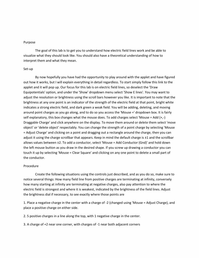
Set-up

Using alligator clips, choose one of the capacitors at your station and hook up the circuit with the

resistor, capacitor, and voltmeter all connected in parallel as shown in the diagram and described by the

lab instructor. Use the resistor labeled R7 on the circuit board, which has a listed resistance of 22,000 Ω

± 5%; the high resistance will prolong the capacitor's discharge making it easier to measure. Do not

attempt to wrap the wire from the capacitor around the prongs of the resistor, just use alligator clips. BE

SURE to connect the capacitor into the circuit properly with the + end (if the capacitor has a polarization

preference) connected to the positive side of the voltage supply, and the – end to the negative side. The

– end should be labeled with a – sign and an arrow pointing to it.

As always, ensure that the voltage control knob is turned completely counter-clockwise at zero before

turning on the power supply and opening the RC LoggerPro template.

Procedure

Zero the reading on the program and turn up the voltage of the power supply to about 5.0 V. Be

prepared to quickly disconnect the + voltage clip lead from the circuit, and then start collecting data. As

soon as the “Collect” button turns red and you see data begin to collect, remove the clip. The capacitor

will begin to discharge through the resistor and you will see the both plots begin to go down, one

following an exponential path with time and the other a downward-sloped straight line. Data collection

automatically stops after 10 seconds. You should turn down the voltage supply to 0 at this point.

Calculations

As you will hear in lecture, a charged capacitor connected to a resistor discharges through the resistor in such a way that the voltage across the capacitor decreases with time according to the equation V(t) = Voe–t/(RC), where Vo is the initial voltage across the capacitor at time t = 0, R is the resistance value of the resistor, and C is the capacitance value of the capacitor. LoggerPro has plotted both V(t) and ln(V(t)) = constant – t/(RC). Whereas V(t) is an exponential, the natural log of the absolute value of V(t) is a straight line of slope magnitude slope = 1/(RC). So the capacitance is equal to C = 1/(R·slope).

On the graph, highlight from near the top of the ln(V(t)) plot (the straight green line) to a point where

the line starts to get noisy(erratic and no longer straight), and perform a least-squares fit. When the

“Select Columns” dialog box opens, deselect “Latest Potential” so that only straight-line graph will be

negative side

positive side

involved. Right click the least-squares data box, open “Linear Fit Options”, and change the settings to

show 5 significant figures and to “Show Uncertainty.” Record your slope and uncertainty values on the

data sheet. Now multiply the reciprocal of the slope magnitude times the manufacturer listed 22,000 Ω

resistance to find the capacitance in the SI unit farads (F). Because the resistance is much too high to

measure with our equipment as you did in lab 3, and because the manufacturer listed uncertainty for

the resistor is 5%, which should be orders of magnitude greater than the uncertainty of your slope

value, the uncertainty of the slope makes no observable contribution to the total uncertainty of the

capacitance. As a result the uncertainty of the capacitance is 5% of your calculation.

More Set-Up

Now the exchange capacitor in the circuit with another one and go through the process again.

Afterwards do it twice more, first with both capacitors connected in parallel, and then with then in

series and record all results. Be careful to always connect the positive side of the capacitor (if polarized)

to the positive side of the voltage supply and zero the reading (with the voltage supply still at zero)

between each experiment.

connected in

parallel

connected in

series

Resistors and Light Bulbs

Introduction

This lab will build on the work you did in lab 3, so you may want to look back to re-familiarize

yourself with how it was done to conserve your lab time. In addition to measuring the resistance of a

single resistor you will be measuring that of multiple resistors connected in series, and again connected

in parallel.

Remember, a series circuit is where multiple resistors are arranged one after the other so that

the current has to travel through both in succession. In this arrangement the combined resistance is

simply the sum of the resistance of the individual resistors. A parallel circuit is where the resistors are

arranged side by side in separate paths so that individual electrons can pass through either and the

current is spread between the two. In this arrangement the combined resistance is Rp = (1/R1 +

1/R2)^−1

Part 1

purpose

The goal of this lab is to measure the resistance of circuits with several types and configurations of

resistors. In so doing you will demonstrate the difference between series and parallel circuits, and you

will show the correlation between calculated values of circuits with multiple resistors. In part 2 of this

lab you will compare the linear carbon resistors to the non-linear resistance of a light bulb.

set-up

First of all make sure the voltage-adjust knob is turned fully CCW (counter-clockwise) whenever you are

not actively taking measurements to avoid accidents. To start with set up a simple circuit exactly as you

did in lab 3 using 1 the 51Ω resistors on the Vernier circuit board. By now you should be familiar with the

equipment, if not you can refer to lab 3 to re-familiarize yourself, or check the Resistor and Light Bulbs

Diagram if you are confused. Once you are certain that your circuit is properly hooked up make sure the

voltage-adjust knob is turned fully CCW before turning on the power supply. Now you are ready to open

the Ohm'sLawSP template, zero the reading and begin collecting data.

procedure

Exactly as you did in lab 3, record 9 data points measuring the voltage and current starting with the

voltage setting at 0V and increasing it to 4V in increments of approximately 0.5V. At each increment

remember to let the system settle for a few seconds and click "keep" to record the measurement. Once

you have all 9 points click "stop" and turn the voltage back to zero.

Calculation

Perform a least-squares fit for your 9 data points and make sure to select "5-significant figures” and

“Show Uncertainties” as in lab 3 and record your slope and uncertainty on the data sheet as they

appear– for the time being you will keep all digits for subsequent calculations. If you did everything

properly, you should find that the slope-value (the resistance of the carbon resistor) has an uncertainty

of only about 0.2% or less! (In the aggregate, these resistors are only specified to a 5% range above and

below the nominal value of each resistor printed on the circuit board.)

more set-up

Now you will repeat the process for different sets of resistors. To clear the graph, on the menu bar click

"Data" and select "Clear All Data". Leave the least squares box open so you don't have to make it again.

Move the alligator clips from the 51Ω resistor to one of the 68Ω resistors and repeat the process of

collecting 9 data points and recording the slope and uncertainty on the data sheet. Once you are done

with both resistors by themselves, hook up the circuit with both resistors connected first in series then

in parallel. Record all calculations on the data sheet.

parallel

series

part 2

purpose

As you have seen, the carbon resistor is AMAZINGLY linear (constant resistance value independent of

the voltage). So are ALL resistors of constant resistance value? Absolutely not! One of the best examples

of a resistor that changes values with applied voltage is the light bulb – as the voltage increases, the

temperature of the filament changes, which causes the resistance to change. The purpose of part 2 is to

see how it does so.

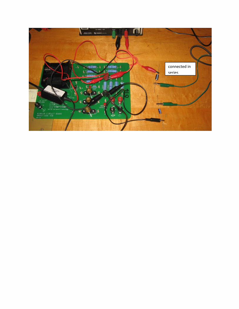
Set-up

Making sure the voltage-adjust knob is set to zero, disconnect the alligator clips from the carbon

resistors and hook up the circuit as you did with the single resistors, this time using the round light bulb

labeled #50 located in one of the three sockets mounted on the circuit board. This time open the

LightBulb.cmbl template and as before zero the measurement and begin collecting data.

Procedure

Record measurements as you have been but with more data points. It is important here to wait several

seconds for the system to reach steady values before recording each data point. Take measurements at

approximate voltages of 0, 0.1, 0.2, 0.3, 0.4, 0.5, 0.6, 0.8, 1.0V, and continue increasing in increments

of .25V up to a maximum of 4.0V. As you are doing this record the minimum voltage where the light

bulb begins to glow on the data sheet. When you are finished click "stop" and turn the voltage

adjustment knob back to zero.

Calculations

Click the m= button on the toolbar. This creates a line tangent to curve made by your data points and

tells you the slope. Move the cursor horizontally to switch between different points keeping an eye out

for 3 things: the maximum and minimum resistance, and the point where the resistance changes most

quickly (the highest slope). When you find them record the resistance and uncertainty at those points on

the data sheet.

Linear vs. Nonlinear Circuits; Magnetic Field Measurements

Introduction

Lab 6 will see you perform 2 very different experiments. For the first you will be building on your work

from last week. You will once again be determining the resistance of both a linear and non-linear circuit,

this time with several resistors connected in both series and parallel. Be sure to review lab 5 because

this lab should test your knowledge of parallel and series circuits, as well as further your understanding

of the differences between linear and non-linear circuits.

In the second experiment you will be making magnetic field measurements using a special device called

a Hall Effect probe, named that way because it uses the “Hall Effect” to make its magnetic field

measurements. All that you need to know about the Hall Effect probe is that it contains a thin, flat wafer

of a semiconductor material and is sensitive to the DIRECTION of the magnetic field as well as its

MAGNITUDE. The wafer is mounted about 1 cm back from the tip of the probe with its SURFACE-

NORMAL parallel to the long axis of the probe. This results in the probe reading the greatest magnetic

field strength (magnitude) when the magnetic field is parallel (or anti-parallel) with the long axis of the

probe. This further means that the probe measures zero field strength when the magnetic field direction

is PERPENDICULAR to the long axis of the probe. This experiment should lead to some interesting

epiphanies regarding magnetism and magnetization.

Part 1

Purpose

To use similar techniques to the ones you have previously demonstrated to examine more complex

circuits, deepening your understanding of the concepts involved.

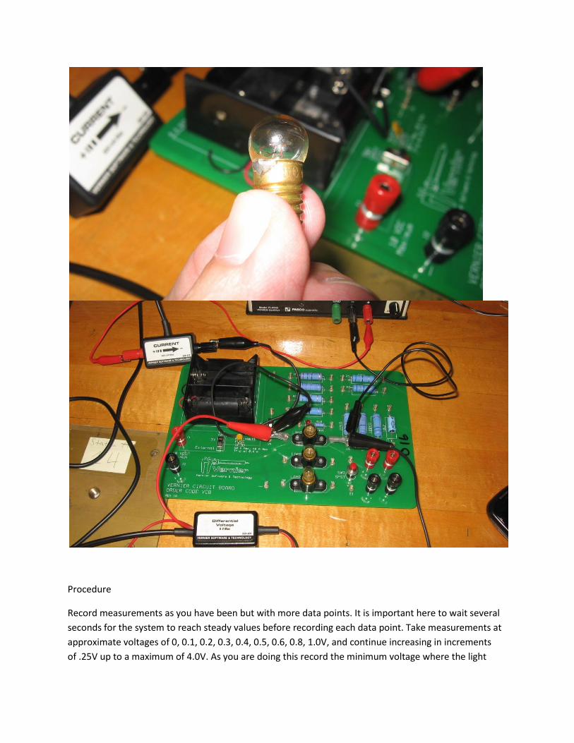
Set-up

Hook up the resistor circuit (as shown in the Circuit Diagram and discussed by your lab instructor)

involving three carbon resistors of labeled values of 10, 51, and 68Ω. Please note that you are to include

as part of the circuit a pair of current sensors for measuring electrical currents through two different

parts of the circuit AND a pair of voltage sensors for measuring the electrical potential difference across

two different parts of the circuit. With these current and voltage measurements, you will be able to

determine the voltage across and current through each of the three resistors. When connecting the

probes to the computer, be aware that the order they are plugged in matters: The first (leftmost)

voltmeter plugged in should be the one measuring across the entire circuit, and the first ammeter

should be the one measuring the beginning of the circuit.

Procedure

Open up the Kirchhoff template, turn the voltage-adjust knob of the power supply fully CCW to the zero position, and then turn the power supply on. Zero the reading and begin collecting data. Use the Keep function to collect data from 0 V to 5 V in 1V increments. Turn the voltage back down to zero when you are finished.

Calculations

Perform a least-squares fit on the upper graph. Right click on the data box that opens up, select “Linear Fit Options,” then choose 5 significant figures and enable “Show Uncertainty”. Record your results on the Worksheet. Do the same with the lower graph, and record those results as well. The I1,V1 data set measures the total values across the entire circuit, so the slope is the equivalent resistance of the entire parallel/series circuit. The result for the I2,V2 data set is the actual measured resistance of the 68 Ω resistor. Note how well the datum points on each graph fit a straight line. Because the carbon resistors are so linear, ALL of the currents and voltages increase linearly as the voltage across the circuit is increased. move your cursor over the upper-right datum point of one of the graphs, and record the I and V values

far that point that appear in the lower left corner of the graph. Do this for both graphs and record the

results on your Data Sheet.

With those two pairs of I,V values, you will be able to calculate the resistance of each of the three

resistors used in the circuit. To do this, go to the Circuit Diagram and next to each resistor in the sketch,

write down the respective voltage across it and the current through it. (Some of these values you have

measured directly. The values not measured you can deduce from the set of measured values. For

example, the voltage across the 51 Ω resistor is your measured V2 value, and the current through the 68

Ω resistor is your measured A2 value. And please be aware that the voltage across the 10 Ω resistor is

NOT equal to the voltage across the entire circuit!) Given the numbers in this sketch, you will be able to

calculate the resistance value of each resistor using Ohm’s law.

More Set-up

Replace the 68Ω carbon resistor with the #50 light bulb that should already be placed in one of the light

sockets (Circuit Diagram 2). Test that all the probes are reading correctly and the bulb is working by

turning up the voltage to about 4 V and back down to 0 V. Zero the readings and take data as you did

before. Notice how the presence of the light bulb changes the shape of the data.

After you've stopped the collection process, turn the voltage supply control knob fully CCW to the 0V

position. In the same manner as before, record the I and V values for the far upper right datum point on

each graph and do the same for the first non-zero datum point on each graph closest to the origin. On

your Lab Report you will be asked to calculate the current through and voltage across each of the 3

resistive elements at both the high- and low-voltage points. This is so that you can calculate a resistance

for each element at both the high and low points in your data set and demonstrate the nonlinear

behavior caused by the light bulb.

Part 2

Purpose

To use the Vernier equipment to demonstrate the Hall effect, and to observe how magnetization can be

easily induced and removed from "soft" magnetic materials.

Procedure

Open the MagField1.cmbl template. Set the range switch on the magnetic field probe to 6.4 mT.

With the magnetic field probe steady on the surface of the lab bench, zero the reading and begin

collecting data. Keeping the magnetic field probe motionless on the bench top, slide the bar

magnet along the table top toward the probe along an extension of the long axis of the probe.

Watch the probe meter reading, and be careful NOT to exceed a magnetic field magnitude of

5 mT (which is just below the upper-reading limit of the magnetic field probe). Move the bar

magnet some distance away, turn it end-over-end, and slide it back directly toward the probe

again. When at a reading of approximately 5 mT magnitude, don’t bring the magnet any closer

but rotate it around its center slowly while watching the magnetic field reading carefully. Rotate

through at least 360°.

Now move the magnet far away from the probe, and this time slide it in along a line perpendicular to

the probe and aimed at a point about 1 cm back from the probe tip(this is where the sensor is). As you

push the magnet closer, adjust the distance of its line of travel either closer or further from the tip in

order to make the probe reading close to zero. Because the magnetic field lines diverge from one

another after leaving the tip of the bar magnet, the magnetic field in the vicinity of the Hall Effect wafer

(inside the probe) will have a small component along the axis of the probe unless the center of the bar

magnet is aimed exactly at the wafer, and by slight adjustment of the bar magnet’s line of travel, you

can aim the center of the bar magnet end directly at the (hidden) wafer, so that the measured field

strength is zero.

At this point you have established that the probe is most sensitive to fields parallel (or

antiparallel) to the probe’s long axis and oblivious to fields that are perpendicular to the long axis

of the probe. (Actually, this field sensitivity varies as the cosine of the angular difference

between the probe axis and the direction of the magnetic field at the wafer.)

Take a paper clip and bring it up to the tip of the probe and turn it end-over-end to ensure that the

paper clip is not magnetized. If it does cause a small reading as you turn it end-over-end, throw

the paper clip vigorously to the floor or against the wall a few times, and that should remove

most of any residual magnetism. (Related admonition: Do NOT drop the permanent magnets on

the floor or on the lab bench. With abuse, even a permanent magnet can lose a bit of its

magnetization.)

Now move the bar magnet to a point some distance away from the probe, and touch one end of

the paper clip to one end of the bar magnet. Holding the paper clip so that it touches the magnet

and sticks straight out straight along the long axis of the magnet, slide this arrangement toward

the probe along the probe’s long axis with the paper clip between the magnet and probe. As the

clip+magnet arrangement approaches the probe a nonzero field value should begin to register,

and as long as the reading never exceeds 5 mT you can bring the free end of the paper clip right

up the flat end of the probe. With the paper clip held firmly in place against the probe, take the

magnet out of contact with the paper clip, bring the magnet back again several times while

watching the probe reading. Repeat the process with the bar magnet turned the other way.

With the clip+magnet touching the end of the probe, leave the magnet in place, and this time remove

the paper clip. Reinsert and remove the paper clip through a few cycles noting the behavior of the probe

reading as you do. Turn the magnet back around so the original side is touching the paper clip again and

do a few more cycles of removing and reinserting the paper clip.

Place the magnet some distance away and touch the paper clip against the probe tip and observe

the probe-reading change as you rotate the clip end-over-end. You should observe that the paper

clip retains some residual magnetization, and you will be asked to describe your observations on

your Lab Report. Now throw the paper clip down on the floor at least two or three times and

repeat the end-over-end measurements as above. What do you observe now?

Here’s the point. In all magnetic materials there are lots of little magnetic domains where all

atoms in a given domain have their microscopic magnetic moments – their tiny bar magnet

equivalents – all lined up in the same direction. In a permanent magnet, all these little domains

can be more or less lined up, giving a large resulting magnetic field. Also these domains tend to

stay lined up for a LONG time unless the temperature of the magnet is raised to a high-enough

level to cause the domains to disalign, or the “permanent” magnet suffers enough dropped-to-

the-floor type abuse. We call such material a “hard” magnetic material (a “hard” magnetic

material requires a LOT of abuse to lose any of its magnetism, but we don’t want our magnets to

lose even 1% – so treat them CAREFULLY). A paper clip, of the other hand, is “soft”. Although

it has domains containing atoms that tend to all be magnetized in the same direction, these

domains only line up cooperatively when an external magnetic field is applied. This alignment

largely disappears when the field is removed. However, “largely” does not mean “completely”.

You’ll no doubt be interested to learn that any residual alignment of domains in soft iron (like a

paper clip) can usually be completely disrupted by a few sharp impacts (like throwing the paper

clip to the floor a few times).

The Magnetic Field

Introduction

In lab 7 you will studying the electric fields produced by solenoids, essentially long coils of tightly packed

wire, which with a current passed through it produces a strong. In a perfect solenoid (one which

stretches to infinity, a little longer than ours) the magnetic field inside the coil is perfectly uniform along

its length, as well as the distance from the central axis, and produce an electric field given by B= μ0nI,

where I is the current, is the rotations in the coil per unit length, and μ0 is a constant. The 400 turn coils

we will be using are not quite so perfect, but they should illustrate the point.

Purpose

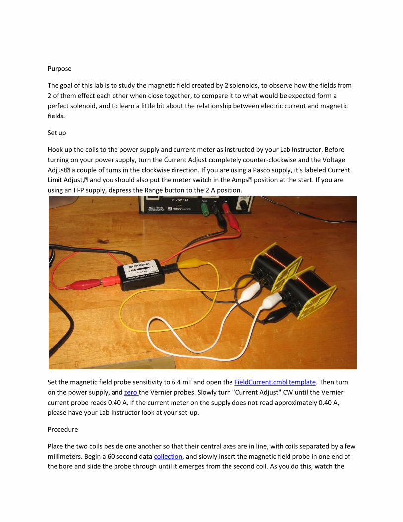
The goal of this lab is to study the magnetic field created by 2 solenoids, to observe how the fields from

2 of them effect each other when close together, to compare it to what would be expected form a

perfect solenoid, and to learn a little bit about the relationship between electric current and magnetic

fields.

Set up

Hook up the coils to the power supply and current meter as instructed by your Lab Instructor. Before

turning on your power supply, turn the Current Adjust completely counter-clockwise and the Voltage

Adjust• a couple of turns in the clockwise direction. If you are using a Pasco supply, it's labeled Current

Limit Adjust,• and you should also put the meter switch in the Amps• position at the start. If you are

using an H-P supply, depress the Range button to the 2 A position.

Set the magnetic field probe sensitivity to 6.4 mT and open the FieldCurrent.cmbl template. Then turn

on the power supply, and zero the Vernier probes. Slowly turn "Current Adjust" CW until the Vernier

current probe reads 0.40 A. If the current meter on the supply does not read approximately 0.40 A,

please have your Lab Instructor look at your set-up.

Procedure

Place the two coils beside one another so that their central axes are in line, with coils separated by a few

millimeters. Begin a 60 second data collection, and slowly insert the magnetic field probe in one end of

the bore and slide the probe through until it emerges from the second coil. As you do this, watch the

magnetic field graph that is being recorded in real time. (Be sure that the probe reading does not exceed

the 6.4 mT level at any time.)

If the coils are creating fields in the same direction, you should see the magnetic field rise to a maximum

value as the probe passes through the first coil, decrease to a relative low point when the field-sensitive

region is halfway between the two coils, and increase again as the probe is slid through the middle of

the second coil. If the coils are creating oppositely directed fields, the field strength at the halfway point

should go through zero and then reverse polarity as you slide the probe through the second coil.

Regardless of which arrangement you start with, slide the probe through the pair of coils at least a

couple of times while recording the field and current readings. Turn the current down to zero, and

reverse the wire connections to just one of the coils, thus reversing its polarity. Turn the current back up

to 0.40 A, and slide the magnetic field probe through both magnets another couple of times, again while

recording the field and current readings.

Now slide the second coil away from the first coil (so that it does not contribute much to the reading of

the probe when the probe is in Coil 1). Zero the probes again, then slide the probe slowly through the

center of the first coil while recording data so that you can obtain a good reading of the maximum field

and corresponding current, which you then should record on your data sheet. Turn down the current to

0.30 A and repeat the above procedure, again recording results on your data sheet. Repeat a third and

fourth time for currents of 0.20 A and 0.10 A.

Introduction

This is the 8th and final lab in PH 1120, and we have 2 very interesting experiments for you to work on.

In the first experiment you will be using the Hall effect probe from the last 2 labs to measure the

magnetic field of the Earth! You will get to see how nature of the probe allows you to not only measure

the magnitude, but also scope out the direction of the magnetic field.

In the final experiment in this class you will be observing an immensely important phenomenon:

electromagnetic induction. As you should already know from lecture, changes in magnetic flux with time

can be used to create a electro-magnetic force, which is the concept behind nearly every power plant on

the planet. This experiment should increase you understanding of induced EMF's and give you practice

in observing their polarity, which should help you to prepare for Exam 4.

Part 1

Purpose

In this experiment you will observe the magnetic field of the Earth using a Vernier magnetic field probe,

finding the direction and strength of the magnetic field vector.

Procedure

Plug the magnetic field probe into the computer and set the sensitivity to 0.3 mT, since the magnetic

field of Earth is too weak to be measured accurately by the higher sensitivity. Open the MagField1.cmbl

template and begin collecting data. During one 60 second recording interval, point the probe in all 3

dimensional directions (including up and down) and make note of the directions of the probe

corresponding to the maximum and minimum magnetic field. They should be in opposite directions. As

you observed last week, the magnetic field probe records its greatest reading when oriented in the

direction of the magnetic field, so this represents the approximate direction of the magnetic field vector

of Earth.

You should find that maximum and minimum readings you just found do not occur in a horizontal

direction. This is because the magnetic field of Earth is similar to what would be produced by having a

long bar magnet spanning the diameter of Earth from the north pole to the south. The field lines should

only be horizontal at the equator. At high latitudes they should have a significant vertical component. In

addition the large quantity of Iron in the structure of Olin Hall distorts the direction slightly, which

should explain if the direction you found is somewhat different from others around the room.

Orient the probe to approximately perpendicular to the orientations you found earlier, so that there

theoretically should be no magnetic field, and zero the reading. Perform another cycle of collecting data,

and this time exhaustively sweep through all directions in the vicinity of both the maximum and

minimum you found earlier. This should get an accurate value for the maximum and minimum field.

Calculation

The difference between the maximum and minimum values for the magnetic field should be equal to

twice the value of the magnetic field of Earth, and if you zeroed the reading correctly the max and min

should have approximately equal magnitudes. Check if your measured field strength is in the vicinity

of .5 = .05 mt (The SI unit is Tesla, but the magnetic field of Earth is usually expressed in the smaller unit

gauss).

Part 2

Purpose

In this experiment you will see how an electro-magnetic force can be induced in a wire when exposed to

a changing magnetic field. You will be using a bar magnet moving through a wire coil to show this.

Set-up

Disconnect the magnetic field probe from the LabPro interface and replace it with a voltmeter. Connect

the red and black leads of the voltmeter to the coil at your lab station, as described by your Lab

Instructor. It may be helpful to extra alligator clips, as the clips from the voltmeter tend to slip off from

the coil. Place the blue foam circular pad on the bench, flat side up, and place the coil on that top flat

surface with the central hole of the coil facing up. Then open the Vernier template labeled

InducedEMF1.cmbl.

Procedure

Click "Collect" to start recording voltage, and then slide the bar magnet at your station rapidly into the

central hole of the wire coil. You should see a voltage spike appear on the recording. Now pull out the

magnet rapidly. You should see another voltage spike, but this time with opposite polarity, why is that?

Experiment with the speed with which you slide the magnet into and out of the coil. In general, the

faster you slide the rod in or out, the bigger the induced EMF will be. As you slow down, however, you

will reach a point where you will see NO effect from the changing magnet field – it’s changing at just too

slow a rate. When the magnetic field is not changing there is no measurable EMF. Turn the magnet

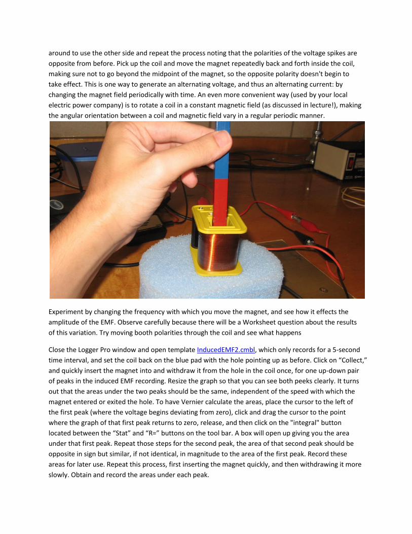
around to use the other side and repeat the process noting that the polarities of the voltage spikes are

opposite from before. Pick up the coil and move the magnet repeatedly back and forth inside the coil,

making sure not to go beyond the midpoint of the magnet, so the opposite polarity doesn't begin to

take effect. This is one way to generate an alternating voltage, and thus an alternating current: by

changing the magnet field periodically with time. An even more convenient way (used by your local

electric power company) is to rotate a coil in a constant magnetic field (as discussed in lecture!), making

the angular orientation between a coil and magnetic field vary in a regular periodic manner.

Experiment by changing the frequency with which you move the magnet, and see how it effects the

amplitude of the EMF. Observe carefully because there will be a Worksheet question about the results

of this variation. Try moving booth polarities through the coil and see what happens

Close the Logger Pro window and open template InducedEMF2.cmbl, which only records for a 5-second

time interval, and set the coil back on the blue pad with the hole pointing up as before. Click on “Collect,”

and quickly insert the magnet into and withdraw it from the hole in the coil once, for one up-down pair

of peaks in the induced EMF recording. Resize the graph so that you can see both peeks clearly. It turns

out that the areas under the two peaks should be the same, independent of the speed with which the

magnet entered or exited the hole. To have Vernier calculate the areas, place the cursor to the left of

the first peak (where the voltage begins deviating from zero), click and drag the cursor to the point

where the graph of that first peak returns to zero, release, and then click on the "integral" button

located between the “Stat” and “R=” buttons on the tool bar. A box will open up giving you the area

under that first peak. Repeat those steps for the second peak, the area of that second peak should be

opposite in sign but similar, if not identical, in magnitude to the area of the first peak. Record these

areas for later use. Repeat this process, first inserting the magnet quickly, and then withdrawing it more

slowly. Obtain and record the areas under each peak.

As a final test, turn the blue foam pad over making sure that it is centered on the black rubber sheet at

your station, and place both well back from the edge of the bench (so that nothing ends up bouncing to

the floor!). Pick up the coil in one hand and hold the magnet vertically suspended over the coil so that

the coil can be dropped through the hole in the coil to land GENTLY in the slot of the blue foam piece.

NOW THIS NEXT IS REALLY IMPORTANT! The coil should be held high enough above the blue piece so

that the magnet does NOT bounce back up anywhere close to the coil, AND the magnet should be held

initially at least an inch above the coil so that it starts out having no effect on the coil. When one partner

has the coil and magnet all lined up, with the magnet ready to drop, the other should click “Collect.”

When the recording starts drop the magnet, and if it drops cleanly through the hole to the foam piece

underneath (and DOESN'T bounce to the floor!!!), that recording should provide good results. (If the

drop wasn’t clean, simply try again.) Determine the area under both the positive and negative peaks in

your recording as before, and record them for use on your Worksheet. Be sure to observe the relative

durations of the two peaks (specifically, are they the same or does one peak have a larger duration than

the other?).

Worcester Polytechnic Institute

Physics Department

PH 1120 - The Electric Field - Lab Report

Your Name & Section: ?

Partner’s Name: ? Date: ?

1. Determine the length and angular orientation of the electric field at the indicated point resulting from the

given 2-charge superposition. State the values and draw an arrow representing the field vector.

2. Solve for the Electric field vector in question 1 again but using Cartesian coordinates. Describe how you

would go about calculating how this value would change if additional points were added

3. Describe 1 change you could make to the diagram in question 1 that would change the field vector in the

following ways, ie. changing charge values, moving or adding a point charge etc. (there may be more than 1

correct answer).

a. Decrease the angle Ɵ by 90 degrees

b. Make the net electric field zero (without removing both charges).

c. Cause the arrow to point to a location 1 unit below where it points in question 1.

j

i

-2

8

Worcester Polytechnic Institute

Physics Department

PH 1120 - Electric Fields & Field Lines Lab Report

Name:_____________; Partner:______________

Section:____________; Date:______________

1. If you were to draw the field lines yourself, and you had a situation with a +10 point charge

in between a -8 point charge and a -4 point charge on either side at equal distances, which

charge would have the most field lines originating or terminating at infinity? What would

you expect the ratios to be?

2. In situation two, describe where the electric field was weakest. You might have expected the

field to be weakest at infinity, explain why it is not.

3. At points very close to a point charge, the field lines should be almost completely unaffected

by other charges. Explain why that is.

4. Is it possible for two electric field lines to ever intersect? Explain.

5. When drawing field lines near conductors (conductors being filled with charge – electrons –

that are free to move around inside the conductor), explain why no field lines are able to

penetrate into the conductor (under electrostatic conditions).

Worcester Polytechnic Institute

Physics Department

PH 1120 - Electric Potential & Determining Resistance Lab

Report

Your Name: ?? Section: ??

Partner’s Name: ?? Date ??

1. Describe the direction of an electric field vector in relation to an equipotential line, and explain why it

is that way.

2. At two random points in a simple circuit, with no resistors or power sources between them, the

potential difference is zero. What does that say about the current and the voltage difference between

them, if anything?

3. Fill out the table below with the results of your four trials, as well as the calculated average and

standard deviation.

Resistance

Values (Ohms)

Uncertainty

(±)

Average

(Ohms)

Standard

Deviation (±)

Worcester Polytechnic Institute

Physics Department

4. Is your standard deviation of the same order of magnitude as the individual slope uncertainties

recorded from each separate experiment? Calculate the ratios of the 4 uncertainties to the standard

deviation. Describe what the two figures represent, and how you would expect the standard deviation

to change with repeated measurements.

5. For each of your slope measurements, are they within they within the sum of that measurement's

uncertainty plus the standard deviation, from the average? What does that say about how accurate the

uncertainties are? Is each measurement with 2 standard deviations of the average? Given the nature of

the standard deviation, how many trials would you have to run before you expect one to be more than

2 standard deviations away?

Worcester Polytechnic Institute

Physics Department

Electric Potential and RC Discharge -- Lab Report

Your Name: ? Partner’s Name: ?

Section: ? Date: ?

1. Using a single point charge of –2, indicate where (how many grid units away) you would place initial

and final points in order to have a potential difference of –3 V. [Note: (

) (

),

begin at page p761and continue through p 770, 13th

edition Young & Freedman and remember that k=1 for our

purposes.]

2. Using a single point charge of –2, indicate where (how many grid units away) you would place initial

and final points in order to have a potential difference of +3 V.

3. Using a single point charge of +8, indicate where (how many grid units away) you would place initial

and final points in order to have a potential difference of –6 V.

4. Using a single point charge of +8, indicate where (how many grid units away) you would place initial

and final points in order to have a potential difference of +6 V.

5. Write down your calculations of the 4 capacitance values in standard format using the 5% uncertainty

discussed in the lab instructions (remember standard format uses one significant figure in the

Worcester Polytechnic Institute

Physics Department

uncertainty unless the lead digit is 1, in which case you use two significant figures, and in either case

you express the main value to the same level of significance as the uncertainty)

6. For circuits with multiple capacitors, those connected in parallel have an effective capacitance equal

to the sum of the value for the individual capacitors. For those connected in series the rule is that the

inverse of the effective capacitance is equal to the sum of the inverses of the individual capacitances.

Calculate the expected capacitances for the parallel and series circuits. Are your calculated values

within the magnitude of the uncertainty of your measured values? Would that still be true if you had

disregarded the 5% uncertainty of the resistor? If so, why do you think that is?

Worcester Polytechnic Institute

Physics Department

PH 1120 - Resistors & Light Bulbs - Lab Report

Name:_____________; Partner:______________

Section:____________; Date:______________

1. In standard form, write down the measured values for all the resistances you measured in the

lab: R1, R2, Rs, Rp, as well as the differential resistances you found in part 2. Remember this

is not the same as what we ask for on exams and summary homework. In standard form the

uncertainty is displayed to one digit, unless the lead digit is one in which case the first 2

digits are displayed. The main value is shown to the same decimal place as the uncertainty.

Notice the difference in the uncertainties for the resistance of the carbon resistors versus

those for the differential resistance of the light bulb, this is because of the number of points

used in the calculations.

2. The equivalent resistance for two resistors connected in series is given by Rs = R1 + R2.

Using your measurements of the individual resistors, calculate the expected value of Rs. Also

calculate the uncertainty using quadrature (the square root of the sum of the squares of the

individual uncertainties, it's just like finding the hypotenuse off a triangle). Compare these

calculated values to the measured values from question 1, the 2 values of Rs should overlap

to within 2 times the uncertainty. This is an important lesson in understanding the industry

standard rules for reporting uncertainty. The uncertainties determined by the least-squares

fitting routine in this experiment represent the precision of their corresponding slope values ,

and the industry-standard rules for presenting numerical results and uncertainties prevent us

from stating more digits than we are entitled to present.

3. Calculate the expected value of the resistance for parallel configuration of resistors using the

equation Rp = (1/R1 + 1/R2)−1

. The rules for calculating the expected uncertainty is much

more complicated here than it was for resistors in a series and is beyond this scope of this

class, so don't bother. Compare your calculated and measured values of Rp using the

measured uncertainty from before and also calculate the percentage deviation between the

two values.

4. State the voltage at which the light bulb first begins to glow. Think about and Describe why

it didn't glow before that.

5. The graph of voltage and current in part 2 clearly doesn't follow a straight line. Why do you

think that is. What do your results say about the light bulb filament and Ohm's law?

Worcester Polytechnic Institute

Physics Department

Linear vs Non-Linear Circuits; Magnetic Field Measurements

Lab Report Your Name: ? Partner’s Name: ?

Section: ? Date: ?

1. Report your least-squares-fit values for both the equivalent circuit resistance and R68 in

industry-standard form (uncertainty rounded to one digit, unless that digit is one, in which

case round the uncertainty to two digits; the main value then rounded to the same place value

as the uncertainty).

2. For the linear circuit, fill in the V, I, and calculated R values for each of the three resistors in

Sketch #1 where indicated. There is enough information to determine everything. (Some of

these I,V values you have measured directly. The values not measured you can deduce from

the set of measured values. For example, the voltage across the 51 Ω resistor is your

measured V2 value, and the current through the 68 Ω resistor is your measured A2 value. And

please be aware that the voltage across the 10 Ω resistor is NOT equal to the voltage across

the entire circuit! Rather, it is the difference V1 – V2.)

Sketch #1

10 Ω

51 Ω 68 Ω

________________ ________

_ ________

_

________________ _________ _________

________________ _________ _________

Worcester Polytechnic Institute

Physics Department

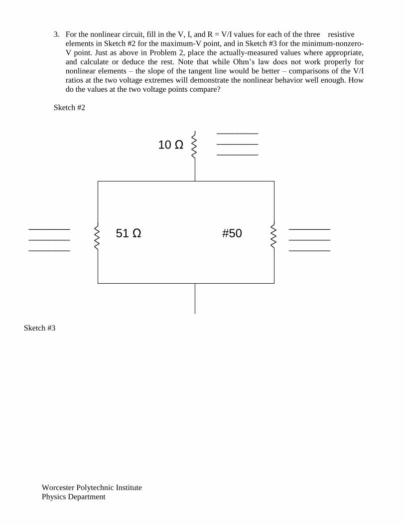
3. For the nonlinear circuit, fill in the V, I, and R = V/I values for each of the three resistive

elements in Sketch #2 for the maximum-V point, and in Sketch #3 for the minimum-nonzero-

V point. Just as above in Problem 2, place the actually-measured values where appropriate,

and calculate or deduce the rest. Note that while Ohm’s law does not work properly for

nonlinear elements – the slope of the tangent line would be better – comparisons of the V/I

ratios at the two voltage extremes will demonstrate the nonlinear behavior well enough. How

do the values at the two voltage points compare?

Sketch #2

Sketch #3

10 Ω

51 Ω #50

________________ _________ _________

________________ _________ _________

________________ _________ _________

Worcester Polytechnic Institute

Physics Department

4. Explain briefly what must be going on with the magnetic field measurement when the

magnet is in a fixed location relative to the Hall Effect probe and a paper clip is slipped in

between the magnet and probe (touching both at either end) and then removed. In other

words, explain briefly your view of why the probe reading changes as the paper clip is

slipped in and out.

5. Explain briefly what must be going on with the paper clip when the probe registers a

magnetic field after the bar magnet is first taken away, but then shows very little magnetic

field after being thrown vigorously to the floor a few times.

10 Ω

51 Ω #50

________________ _________ _________

________________ _________ _________

________________ _________ _________

Worcester Polytechnic Institute

Physics Department

PH 1120 - The Magnetic Field - Lab Report Your Name: ? Partner’s Name: ?

Section: ? Date: ?

1. From the data on your Data Sheet, calculate the ratio of maximum magnetic field to

corresponding current for each of the four pairs of values recorded. Does the maximum field

value at least approximately scale in linear proportionality with the current?

2. For the coil used in your experiment, there were 400 windings in a span of 3.9 cm. Calculate

the magnetic field you would expect to measure inside an infinitely-long solenoid of winding

density 400 turns per 3.9 cm carrying a current equal to the greatest current value on you

Data Sheet.

3. As an added calculation arising from Problem 2, calculate the percent deviation of your

measured maximum magnetic field from that predicted by the ideal solenoid equation.

(Because the coil you used is quite short, your measured maximum field should be about

80% of the solenoid prediction – maybe even a bit more than 80%. Is it?)

4. Describe what would happen to the magnetic field produced if you were to apply an

oscillating current through the coil. How do you think that would affect the voltage across the

coil?

5. A perfect solenoid generates a perfectly uniform magnetic field at all points. Briefly describe

why that is, and why our short coil doesn't quite do the same things.

Worcester Polytechnic Institute

Physics Department

PH 1120 - Electromagnetic Induction - Lab Report Your Name & Section: ?

Partner’s Name: ? Date: ?

1. State the value of your measurement of the magnitude of the Earth’s magnetic, and describe

the direction of the field that you observed at your station. Which of these directions

represents north? How would you expect the vertical component of the direction to change at

different point on the globe?

2. Consider the magnetic induction situation when the magnet is rapidly inserted into a coil,

held motionless, and then rapidly removed from the coil. Explain the forces and phenomenon

involved in this 3-step process, and explain why the polarities of the resulting EMF's are

different.

3. Now compare the situation in Prob. 2 above with the identical situation with the magnet

turned end-for-end. Compare the polarities of the induced EMFs in these two situations, and

explain briefly the reasons behind the polarities observed.

4. Consider the situation where you moved the magnet back and forth in the coil in periodic

fashion, thus inducing a periodic EMF in the coil. Specify the kind of periodic motion that

led to the induced EMF of largest amplitude (rapid back-and-forth, or less rapid back-and-

forth motion). Explain the physical reason for this observed behavior.

5. From the part of the experiment where you found the area under the curves of the graph of

the EMF, calculate the average of the three areas corresponding to the magnet going into the

coil, and then find the maximum percent deviation from this average of the 3 trails. Then do

the same for the 3 areas corresponding to the magnet being removed from the coil. Explain

why the area should be independent of the rate at which the magnet is moved.

Conclusion

In summary, the improvements I have made to the PH1120 labs should help to improve

the students overall learning experience. By being more engaging and more explicit in their

instructions, they should reduce any confusion students may have and help them to complete

their work more quickly and easily. They should also increase the students' understanding of the

material. Additionally the TA's should have to answer fewer questions and fix fewer student

mistakes so that lab times will be more productive and should be completed more quickly.