improving manufacturing systems using integrated discrete event simulation and evolutionary

Improving Manufacturing Systems Using

Integrated Discrete Event Simulation

and Evolutionary Algorithms

Parminder Singh Kang

A Thesis Submitted in Partial Fulfilment of the Requirement of De Montfort

University for the Degree of Doctor of Philosophy

May 2012

De Montfort University

i

Abstract

High variety and low volume manufacturing environment always been a challenge for

organisations to maintain their overall performance especially because of the high level

of variability induced by ever changing customer demand, high product variety, cycle

times, routings and machine failures. All these factors consequences poor flow and

degrade the overall organisational performance. For most of the organisations,

therefore, process improvement has evidently become the core component for long term

survival.

The aim of this research here is to develop a methodology for automating operations in

process improvement as a part of lean creative problem solving process. To achieve the

stated aim, research here has investigated the job sequence and buffer management

problem in high variety/low volume manufacturing environment, where lead time and

total inventory holding cost are used as operational performance measures. The research

here has introduced a novel approach through integration of genetic algorithms based

multi-objective combinatorial optimisation and discrete event simulation modelling tool

to investigate the effect of variability in high variety/low volume manufacturing by

considering the effect of improvement of selected performance measures on each other.

ii

Also, proposed methodology works in an iterative manner and allows incorporating

changes in different levels of variability.

The proposed framework improves over exiting buffer management methodologies, for

instance, overcoming the failure modes of drum-buffer-rope system and bringing in the

aspect of automation. Also, integration of multi-objective combinatorial optimisation

with discrete event simulation allows problem solvers and decision makers to select the

solution according to the trade-off between selected performance measures.

iii

Acknowledgments

In my humble acknowledgement, I would like to convey my gratitude to all the people

who were with me directly or indirectly throughout this long journey.

First and foremost, I wish to thank god who has guided me throughout this journey as

being always with me as strength, determination and courage to pursue this work with

high level of confidence and commitment.

At the professional and academic level, I am really grateful to Dr Riham Khalil and Prof

Dave Stockton (my supervisors) to provide me this opportunity at first instance to work

on this research problem. Essentially, it was impossible to achieve this without their

precious encouragement, advice and guidance and endless support, who never accepted

less than my best effort. Thanks Riham and Dave for your endless guidance and support

in this journey, It is been a pleasure working with both of you.

Especial thanks to De Montfort University and Technology Strategy board to fund this

project (TSB K1532G, Accelerating process excellence using virtual discrete event

process simulation), which enabled me to peruse this research and to all project

collaborates for their valuable feedback.

At personal, I would like to show gratitude to my father and mother for their continuous

support and encouragement, and to my brother who’s endless support allowed me to

focus on my studies, thanks for being there as my elder brother. Words fail to express

my appreciation to my wife whose love and persistence confidence in me, has

encouraged me and always taken-off stress from my shoulders.

iv

I wish to express deep gratitude for all my family members in UK and India for their

love and support. Very special thanks to my uncle Baljit Singh for his invaluable

guidance and has always been a real inspiration to me.

It is a pleasure to thank my second and special family at the lean research group/centre

for manufacturing for their support, suggestions and care. Especially, thanks to

Lawrance Mukhongo for all the great time we spend together and always being there as

my elder brother.

Finally, I would like to thank everybody who was important to the successful realisation

of the thesis, as well as expressing my apology that I could not mention personally one

by one.

v

Declaration

I declare that the work described within this thesis was originally undertaken by me,

(Parminder Singh Kang) between the dates of registration for the degree of Doctor of

Philosophy at De Montfort University, July 2009 to May 2012.

vi

Abstract i

List of Tables xi

List of Figures xiv

Abbreviation and Glossary xvii

Research Dissemination xix

Chapter 1 – Introduction

1.1 Introduction 1

1.2 Need of Synchronous Flow 3

1.3 Lean Philosophy in Synchronous High Variety/Low Volume Manufacturing 4

1.4 Simulation and Combinatorial Optimisation 5

1.5 The Scope of Research 6

1.6 The Aim and Objective 7

1.7 The Structure of Thesis 8

Chapter 2 – Lean Creative Problem Solving and Process Improvement

2.1 Introduction 12

2.2 Brief History of Manufacturing Systems 12

2.3 Lean Philosophy 13

2.3.1 Lean’s Five Principals 15

2.3.2 Waste in Lean 18

vii

2.4 Manufacturing Problems 23

2.5 Lean Creative Problem Solving 26

2.5.1 Characteristics of Effective Problem Solving Process 26

2.5.2 Existing Problem Solving Methods 29

2.5.3 Process Improvement Using Lean Creative Problem Solving Process 34

2.6 Summary 36

Chapter 3 – Combinatorial Optimisation for Process Improvement

3.1 Introduction 37

3.2 Root Cause Analysis as Part of Process Improvement 38

3.2.1 Existing Root Cause Analysis Methods for Process Improvement 39

3.2.2 Process Improvement (PI) 43

3.2.3 Process Improvement Issues 45

3.3 Multi-Objective Optimisation 48

3.3.1 Genetic Algorithms 48

3.3.2 Genetic Algorithm’s Overview 50

3.3.2.1 String Encoding and Objective Function 51

3.3.2.2 Initialisation 52

3.3.2.3 Parent Selection 54

3.3.2.4 Crossover 55

3.3.2.5 Mutation 55

viii

3.3.2.6 Inversion 56

3.3.2.7 Replacement Strategy 56

3.3.2.8 Evaluation 57

3.3.3 Multi-Objective Combinatorial Optimisation 57

3.3.3.1 Existing Multi-Objective Optimisation Approaches 60

3.3.3.2 Proposed Combinatorial Optimisation Framework 63

3.4 Performance Measure (PM) 64

3.5 Summary 66

Chapter 4 – Research Methodology

4.1 Introduction 68

4.2 Research Methodologies Overview 70

4.2.1 Quantitative Research 70

4.2.2 Qualitative Research 72

4.2.3 Triangulation 73

4.3 Research Methodology 73

4.3.1 Discrete Event Simulation Model 74

4.3.2 Multi-Objective Combinatorial Optimisation Model 76

4.4 Proposed Research Framework 77

ix

Chapter 5 – Experimental Results

5.1 Introduction 88

5.2 Experimental Results 89

Chapter 6 – Discussion

6.1 Introduction 119

6.2 Ability to Respond Quickly to the Variability without Compromising the

Organisational Goals 120

6.3 Achieving the Synchronous Flow to Improve the Performance of System in

HV/LV Manufacturing Environment 121

6.4 Contributions of Proposed Methodology 124

6.5 Discussion of Results 129

6.6 Improving Different Performance Measures (PM) by Reducing the Effect of

Variability 135

6.7 Applicability of Proposed Model with the Existing Systems 136

6.8 Adoption of Proposed Method in Different Industrial and Service Sectors 141

Chapter 7 – Conclusion 143

Chapter 8 – Future Work 146

References 148

Bibliography 166

x

Appendix A – Before and After Optimisation Results 169

Appendix B – Developed Graphical User Interface for Combinatorial

Optimisation (SIM-Prove)

187

Appendix C – Optimisation Model Implementation 190

xi

List of Tables

Chapter 2 Lean Creative Problem Solving and Process Improvement

Table 2.1 Traditional Manufacturing System Conditions 24

Chapter 3 Combinatorial Optimisation for Process Improvement

Table 3.1 GA Characteristics 50

Table 3.2 Selection Process 54

Table3.3 Replacement Strategy 57

Table 3.4 Characteristics of Performance Measures 66

Chapter 4 Research Methodology

Table 4.1 Simulation Parameters 78

Table 4.2 Simulation Modelling Element’s Attributes 79

Table 4.3 Product Quantity with Different Work Types 81

Table 4.4 Product Mix with Different Routings 81

Table 4.5 Selected Performance Measures 84

Table 4.6 Combinatorial Optimisation Rules 87

Chapter 5 Experimental Results

Table 5.1a Average Queuing Time and Average Queue Size for 500 Jobs

and Batch Size 1, 5 and 10 91

Table 5.1b % Working, % Waiting, % Changeover and % Stopped for

500 Jobs and Batch Size 1, 5 and 10 92

Table 5.2a Average Queuing Time and Average Queue Size for 1000

Jobs and Batch Size 1, 5 and 10 93



Table 5.3a Average Queuing Time and Average Queue Size for 2000 95

xii

Jobs and Batch Size 1, 5 and 10



Table 5.4 Lead Time and Total Inventory Holding Cost Before and

After Optimisation for 500 Parts 104





Chapter 6 Discussion

Table 6.1 Optimal Production Technology Rules 137

Table 6.2 Theory of constraints Rules 138

Appendix A Before and After Optimisation Results

Table A.1a Average Queuing Time and Average Queue Size for Before

and After Optimisation for 500 jobs and batch size 1 169

Table A.1b % Working, % Waiting, % Changeover and % Blocked for

Before and After Optimisation for 500 jobs and batch size 1 170










and After Optimisation for 1000 jobs and batch size 1

175


Before and After Optimisation for 1000 jobs and batch size 1

176



177

xiii



178



179



180



181



182



183



184



185



186

xiv

List of Figures

Chapter 2 Lean Creative Problem Solving and Process Improvement

Figure 2.1 Lean Creative Problem Solving 34

Chapter 3 Combinatorial Optimisation for Process Improvement

Figure 3.1 Proposed Combinatorial Optimisation Model 51

Chapter 4 Research Methodology

Figure 4.1 Proposed Research Framework 77

Chapter 5 Experimental Results

Figure 5.1a Total Inventory Holding Cost vs. Average Queuing Time 97

Figure 5.1b Lead Time vs. Average Queuing Time 97

Figure 5.2a Total Inventory Holding Cost vs. Average Queue Size 98

Figure 5.2b Lead Time vs. Average Queue Size 98

Figure 5.3a Total Inventory Holding Cost vs. %Working 99

Figure 5.3b Lead Time vs. %Working 99

Figure 5.4a Total Inventory Holding Cost vs. % Waiting 100

Figure 5.4b Lead Time vs. % Waiting 100

Figure 5.5a Total Inventory Holding Cost vs. % Changeover 101

Figure 5.5b Lead Time vs. % Changeover 101

Figure 5.6a Total Inventory Holding Cost vs. % Stopped 102

Figure 5.6b Lead Time vs. % Stopped 102

Figure 5.7a Average Queuing Time before and after Optimisation for 500

Parts without Machine Failure

105

Figure 5.7b Average Queue Size before and after Optimisation for 500


105

xv

Figure 5.7c % Working, % Waiting, % Changeover and % Blocking before

and after Optimisation for 500 Parts without Machine Failure

106


Parts with Machine Failure

107



107


and after Optimisation for 500 Parts with Machine Failure

108



110



110



111



112



112



113



115



115



116



117



117



118

xvi

Chapter 6 Discussion

Figure 6.1 Lead Time before and after optimisation for Batch Size = 1 and

Customer Demand = 500 Parts

123

Figure 6.2 Total Inventory Holding Cost before and after optimisation for

Batch Size = 1 and Customer Demand = 500 Parts

123

Appendix B

Developed Graphical User Interface for Combinatorial

Optimisation (SIM-Prove)

Figure B.1 Setting the Simulation Parameters for Optimisation Process 187

Figure B.2 Genetic Algorithms Optimisation Parameters 188

Figure B.3 Genetic Algorithms Optimisation Results 189

xvii

Abbreviations and Glossary

% Blocked The condition requiring a WorkCentre that has parts to

process to remain idle as long as the queue to which the

parts would be sent is full or waiting for succeeding

WorkCentre to finish the job.

% Changeover It is the waiting time for succeeding workstations that

are waiting for the proceeding workstations to finish the

jobs.

% Stopped It the time work is paused for either short or long term

Interruptions, for instance machine failure.

% Waiting It is the waiting time for succeeding workstations that

are waiting for the proceeding workstations to finish the

jobs.

% Working It is the percentage of time when the WorkCentre is

working

BS Buffer Size

CCR Capacity Constrained Resource

CPI Continuous Process Improvement

CPS Creative Problem Solving

CPSI Canadian Patient Safety Institute

DBR Drum-Buffer-Rope

DES Discrete Event Simulation

DOE Design of Experiments

FJSP Flexible Job-Shop Scheduling Problem

GA Genetic Algorithms

HV/LV High Varity Low Volume

JIT Just-in-Time

JS Job Sequence

xviii

KT Kepner-Tregoe

LT Lead Time

ME Modelling Element

MOO Multi-Objective Optimisation

MTTF Mean Time to Failure

MTTR Mean Time to Repair

OF Objective Function

OPT Optimal Production Technology

PC Paired Comparison

PI Process Improvement

PM Performance Measure

RC Root Cause

RCA Root Cause Analysis

TIHC Total Inventory Holding Cost

TOC Theory of Constraints

TPM Total Productive Maintenance

TPS Toyota Production System

TQM Total Quality Management

TSB Technology Strategy Board

VSM Value Stream Mapping

WIP Work-in-Progress

xix

Research Dissemination

Kang, P. S., Khalil, R. and Stockton, D. (2012) A Multi-Objective Optimization Approach

Using Genetic Algorithms to Reduce the Level of Variability from Flow Manufacturing.

Proceedings of IEEE International Conference on Engineering Technology and Economic

Management, 21 – 22nd May, 2012, Zhenzhou, China, pp. 115 – 119.

He, Y., Ma, W. and Kang, P. S. (2012) On Semi-Bent Functions Niho Exponent, Journal of

China Information Sciences Vol. 55, Issue 7, pp. 1624 – 1630.

Kang, P. S., Singh, G. P. and Sidhu, R. S. (2011) A Descriptive Review of Genetic

Algorithms in Industrial Process Improvement. Proceedings of the International Conference

on Recent Advances in Electronics & Computer Engineering, Eternal University, India, Dec.

2011, pp. 1 – 4.

Kang, P. S. (2011) Use of Genetic Algorithms in Manufacturing Operations Planning. De

Montfort University Research Degree Showcase. May, 2011.

Singh, G. P., Singh, P. and Kang, P. S. (2011) Cloud Server – An Emerging Technology of

Virtualization. Seminar on the Advancements in Computer Technology, Institute of

Engineering and Technology, Bhaddal, India, April. 2011.

Kang, V. K., Kang P. S. and Gupta, M. (2010) Descriptive Review of OSPF. Coimbatore

Institute of Information Technology International Journal of Networking and Communication

Engineering, August, 2010.

Kang, P. S. (2010) Problem Solving Optimisation Using Root Cause Analysis and Genetic

Algorithms, De Montfort University Research Showcase, May, 2010.

xx

Kang, P., Khalil, R. and Stockton, D. (2010) Integration of Design of Experiments with

Discrete event Simulation for Problem Identification. Proceedings of the International Junior

Scientist Conference, April, 2010, Vienna, Austria, pp. 69 – 70.

Khalil, R., Kang, P. and Stockton, D. (2010) Integration of Discrete Event Simulation with

an Automated Problem Identification. Proceedings of International Multi-Conference of

Engineers and Computer Scientists, 13 – 15 Mar., 2010, Hong Kong, pp. 1051 – 1054.

1

Chapter 1 – Introduction

1.1 Introduction

Increased competition in global markets has augmented the manufacturing problems.

This has amplified the need of new, efficient and effective tools and techniques to cope

with these problems. To compete with global economy organisations have to lower the

operational expenses and lead times (LT) by maintaining ever-changing product variety

according to the market/customer demand.

According to Alford et al. (2000), increased product and process variability has caused

escalating cost and complexity in manufacturing systems. High variety/low volume

(HV/LV) manufacturing environment always remained one of the combats that have

kept organisations in the quest of process improvement (PI). Furthermore, there are

numerous entities involved within the manufacturing environment and most of these

entities exhibit dynamic, unpredictable and complicated relationships among them. This

even makes PI more vulnerable to failures as the effect of improving one performance

measure (PM) need to be considered on other PMs before deciding over the optimal

solution. For instance, HV/LV brings numerous challenges for the manufacturers at the

2

operational level to maintain overall performance, such as maintaining lower LTs and

operational cost (Nazarian et al., 2010).

Although high product variety brings a great deal of challenges for organisations at

operational levels to maintain lower LTs and operational cost. However, at the same

time, product variety is designated as one of the most important factors to have a

competitive edge in the global market by offering products and services tailored to a

specific market segment. According to Berry and Cooper (1999), adding product variety

within the customer order can have adverse effect on operational cost and LTs, as

products may have variable setup times, processing times and even follow different

routes. Over the years, numerous techniques have been proposed in implantation of lean

problem solving literature, researchers have regarded synchronous flow as one of the

most effective tools to maintain the high level of organisational performance by

improving the flow of material/information throughout the organisation (Nazarian et al.,

2010; Fresco, 2010; and Naidu, 2008).

This research, therefore, has proposed a methodology for automating the operations

process improvement as a part of lean creative problem solving (CPS) and continuous

process improvement by reducing the effect of variability. To achieve the research aim,

3

proposed methodology addresses the issue of job sequencing and buffer size

optimisation to reduce the lead time (LT) and total inventory holding cost (TIHC).

1.2 Need of Synchronous Flow

Researchers have identified unexpected disturbances as different levels of variability;

for instance, machine breakdowns, variable setup and processing times, ever-changing

customer orders and quality problems that can interrupt the flow of material through the

system, and organisations pay back as increased operational cost and higher LTs

(Nazarian et al. 2010). According to Khalil et al. (2008), disturbances can also be drawn

from the constrained resource (bottleneck), as a bottleneck limits the capacity of the

whole line. In HV/LV manufacturing, it becomes utmost important to reduce the

disturbances because of the product variability involved due to different product types

and product quantities. Researchers have proposed various techniques to achieve the

synchronous flow such as optimal production technology (OPT), Drum-Buffer-Rope

(DBR), buffer management, theory of constraints (TOC) and pull system. Effective use

of such techniques requires an extensive knowledge of variability inherited into each

task and WorkCentre and effect of variability on individual resource utilisation (Khalil

et al., 2008; Wei et al., 2002; and Linhares, 2009).

4

1.3 Lean Philosophy in Synchronous High Variety/Low Volume Manufacturing

According to Shah and Ward (2003), lean philosophy presents a multidimensional

approach that encompasses a wide variety of manufacturing practices, such as just-in-

time (JIT), quality control, cellular manufacturing, supplier management and continuous

process improvement. In HV/LV manufacturing environment, Synchronous flow and

lean philosophy mutually derives PI to reduce the effect of process variability.

According to Khalil et al. (2008), synchronous flow processing is an essential part of

lean philosophy as it provides the infrastructure of pull production and focuses on waste

elimination. For instance, there are a number of strategies that have been applied to

reduce the effect of variability, such as (Khalil et al., 2008; and Nazarian et al., 2010);

a. Line balancing for effective allocation of tasks.

b. Job sequencing to improve the material flow through the setup reductions.

c. Material flow control and use of flexible resources to reduce the effect of

variability.

d. Applying the lean based techniques to reduce the level of variability from the

individual causes.

e. Buffer management to support the cause of variability due to expected (setup’s)

and unexpected (machine failures) causes.

5

In this research, a job sequencing and buffer management problem has been addressed

to reduce the effect of variability. Along this, research here has used the effect of

improvement of different PMs on each other during the PI.

1.4 Simulation and Combinatorial Optimisation

The main motive of this research is to provide a novel method for PI using

combinatorial optimisation and simulation modelling, which may assist organisations to

reduce/manage the effect of process variability. As discussed earlier, under the proposed

methodology, job sequencing and buffer size optimisation problem has been

investigated as a part of PI by reducing the effect of variability. In this research, the

main causes of variability are ever-changing customer demand in product quantity and

type, variable processing times, variable setup times, machine failures and product

routings.

At initial stage, research here has used the drum-buffer-rope (DBR) concept to identify

the constraints in the system and a combinatorial optimisation based solution has been

purposed using Multi-Objective Genetic Algorithm (GA) integrated with Discrete

Event Simulation (DES).

6

Along this, research here has inherited some of the practices of lean philosophy, which

are;

a. Process improvement (PI).

b. Root cause analysis (RCA).

c. Synchronous flow by reducing the effect of variability.

d. Reducing the non-value-added activities.

e. Response to customer demand.

1.5 The Scope of Research

As a part of PI, the main focus of research is to develop an automated lean CPS

methodology to cope with the variability exists in the HV/LV manufacturing

environments. Proposed methodology is tested on a model representing working area at

Perkins. However, proposed methodology can be equally applicable in different

manufacturing and service sectors (Section 6.8) as well as can be used investigating the

different PMs (Section 6.6).

The proposed model can be exemplified on the two major issues involved in

manufacturing systems, which are;

a. Reducing the effect of variability to achieve the synchronous flow.

7

b. Investigating the knock-on effect of performance measures on each other in

process improvement.

1.6 The Aim and Objective

The aim of the research is to develop a novel methodology for automated lean CPS as a

part of operation’s process improvement. The research here will accomplish different

objectives to address the main aim of research. These objectives are;

a. Development of

I. Buffer management system that can operate effectively under the light

of highly variable environment.

II. Addressing the issue of job sequencing to reduce the number of setups

required in the high variety/low volume manufacturing through different

operational level performance measures.

III. Genetic algorithms based multi-objective combinatorial optimisation

methodology to determine the optimal buffer sizes and job sequence in

order to reduce the effect of variability and to promote the synchronous

flow.

8

b. Determining the effect of performance measures on each other during the

optimisation process to bring in the aspect of root cause analysis.

c. Development of an integrated approach using genetic algorithms based

combinatorial optimisation and discrete event simulation modelling to

accommodate rapid changes in manufacturing environment and addressing the

issue of bottleneck and its failure modes in complex high variety/low volume

manufacturing environment.

d. Development of genetic algorithms based combinatorial optimisation

methodology to address the issue of different types of variability in high

variety/low volume complex manufacturing environment, for instance, change

in customer demand, variable setup and processing times.

1.7 The Structure of Thesis

Including an introduction, the research is divided into eight chapters. This section

provides the summary of each chapter.

Chapter 1 gives brief introduction to the research and background for the selected

research topic. Along this, it highlights the aim and objectives for the research.

9

Chapter 2 exemplifies the core component of research, i.e. the lean philosophy, which

will provide a platform to derive the research towards its main aim. It starts by

providing literature review about the lean philosophy, which includes the concept of

lean manufacturing, lean’s five principles and waste in Lean. Further, Chapter 2

exemplifies the fundamentals of the research problem, i.e. manufacturing problems due

to high variety and low volume. This will provide the basis to explore the different

factors that can affect the HV/LV manufacturing environments. Finally, the concept of

the lean CPS and the characteristics of an effective problem-solving process have been

exemplified, which can be utilised in the proposed research method. Along this, chapter

2 illustrates lean CPS as a part of process improvement (PI).

Chapter 3 illustrated the concept of GA based multi-objective combinatorial

optimisation and RCA in context of process improvement. Chapter 3 starts with

introduction and followed by exemplification of RCA in context of PI. Further, it

illustrated the process improvement issues with respect to the main research problem,

i.e. buffer size and job sequence optimisation problem. Next, chapter 3 illustrated the

GA based multi-objective combinatorial optimisation, where GA implementation has

been elaborated with respect to the research problem, i.e. problem encoding, genetic

operators, objective functions (OF) and evolution process illustration using research

10

problem (batch size and job sequence). Finally, chapter illustrates the concept of PM

concept, as PMs are an integral part of this research for quantification and analysis.

Chapter 4 exemplifies the steps undertaken to develop the research methodology. It

illustrates the concept of different research methodologies such as qualitative,

quantitative and triangulation. In this research, triangulation research methodology has

been used to inherit the benefits of both qualitative and quantitative. Further, DES

concept and optimisation model have been described in context of the proposed research

methodology. Finally, chapter 4 elaborates the proposed research framework, where a

GA based multi-objective combinatorial optimisation model has been developed. Along

this, proposed optimisation model is integrated with the discrete event simulation tool

(Simul8) to respond to quick change in customer demand.

Chapter 5 shows the results based on the data collected using proposed methodology.

Chapter 5 exemplifies the results according to the different type of variability, as

defined in Chapter 4. First, this chapter illustrates the failure to identify the bottleneck

using the traditional DBR approach, where correlation analysis is used to identify the

effect of different PM on each other in order to identify the bottleneck resource. Finally,

post optimisation results have shown the improvement through proposed GA based

multi-objective combinatorial optimisation model.

11

Chapter 6 exemplifies the results and the contribution of research towards the existing

knowledge. Result’s discussion has been included based on the PMs identified in

Chapter 4 and according to the data collected using different types of variability. This

chapter discusses the implementation of proposed methodology by considering the

following core components;

a. Implementation of proposed methodology to achieve synchronous flow as a part

of PI in HV/LV manufacturing.

b. Contribution of research towards the existing knowledge.

c. Discussion of results based on the data presented in chapter 5.

d. Reducing the effect of variability by improving different PMs.

e. Applicability of proposed methodology within existing systems.

f. Adoption of the proposed model in different industrial and service sectors.

Chapter 7 concludes the research findings and summarises the contribution of research

in existing knowledge.

Chapter 8 exemplifies the various improvement factors, which can be exploited further

to add value to proposed model, which provides the foundation for continuous

improvement.

12

Chapter 2 – Lean Creative Problem Solving and Process Improvement

2.1 Introduction

This chapter starts with the brief history of the manufacturing systems then exemplifies

the concept of the lean philosophy, where lean’s five principals and seven wastes have

been discussed in context of current research. Further, chapter moves to the modern

manufacturing system problems and their inability to deal with high product variety at

low volume. Finally, this chapter elaborates the concept of lean creative problem-

solving (CPS), where the characteristics of the effective problem-solving process are

taken into consideration for the development of research methodology. Also, this

chapter discusses the implementation of lean CPS as the part of process improvement

(PI).

2.2 Brief History of Manufacturing Systems

In early twentieth century, craft production system failed to cope with dramatically

increased customer demand of cars. As, skilled workforce was spending longer times to

produce a single vehicle, which decreased the throughput and increased the production

cost. These pitfalls of the craft manufacturing system inspired two major industrial

revolutions. The first manufacturing revolution is known as the mass production system,

13

developed by Henry Ford and the second manufacturing revolution was Toyota

Production System (TPS), which further matured into the lean manufacturing

philosophy and widely adopted by many organisations to reap its benefits. Lean

manufacturing combines the concept of craft production and mass production, i.e. high

flexibility at lower cost. For example, it employs teams of multi-skilled workers at all

levels of organisation and uses highly flexible and automated machines for high variety

production.

2.3 Lean Philosophy

Lean thinking is evolved from the TPS, which was introduced in early 1950s’. TPS

introduced a unique engineering approach that focused on continuous organisational

improvement by targeting smooth material flow, flexible operations, waste elimination,

quality and productivity improvement. TPS epitomised the concept of PI through people

involvement in the problem-solving and decision-making process (Burkitt et al., 2009).

According to Ohno (Taiichi Ohno is known as the father of the TPS), quality control,

quality assurance and respect for humanity are the three main factors involved in waste

elimination and PI (Ahuja and Khamba, 2008).

14

Over the last four decades, lean production has become an integral part of

manufacturing landscape by providing improved performance and competitive

advantages (Shah and Ward, 2007). This research here has investigated the problem of

job sequence and buffer sizes as a part of PI to improve production performance by

reducing the non-value added activities to fulfil customer demand under high level of

variability.

Mckellen (2005) has defined lean as, “a production system that considers expenditure of

resources for any goal and service (production for customer) except waste”.

Similarly, Kilpatrick (2003) has exemplified lean as, “A systematic approach to

identifying and eliminating the waste through continuous improvement flow of the

product at the pull of the customer in pursuit of perfection”.

Researchers have regarded lean as a total business philosophy that can be applied to all

aspects and types of manufacturing environments, where the main focus remains to

develop a highly efficient customer focused and streamlined system by removing the

non-value added activities (Al-Kabbi et al., 2009; and Al-Kabbi et al., 2010). Similarly,

lean manufacturing tools are equally applicable to the process of problem solving, as it

assists the attribution of the problem to its causes that can lead to fast and significant

15

definition of root cause (RC) of the problem (Dhafr et al., 2006). Along this, Bhasin and

Burcher (2006) have illustrated that lean can be used at different levels of organisation

for problem solving to investigate the non-value added activities in terms of seven lean

wastes, and this process can derive the organisation towards a common goal of

improved lead times (LT), increased productivity and quality, reduced inventory cost

and work-in-progress (WIP) and higher customer satisfaction. In addition, the solution

to the problem can be standardised and sustained to achieve the long term PI goals. At

the same time, to reap the benefits of lean philosophy it is essential to understand

product and production process variations as these are subjected to diverge according to

change in customer or market demand and supply (Liker and Lamb, 2000).

This highly dynamic and rapidly changing manufacturing environment has increased

the manufacturing problems at the operational level; for instance, some of these

manufacturing problems are illustrated in Section 2.4. This research has investigated the

job sequence and buffer size problems as a part of PI under the high level of variability.

2.3.1 Lean’s Five Principles

Khalil (2005) has summarised lean thinking in five lean manufacturing principles; these

are:

16

a. Identify Customers and Specify Value – this defines the concept of specifying

the value from the customer point of view. Production process can be defined

and analysed with respect to customer values, where a customer can be internal

or external. As, only a small fraction of the total time and effort in any

organisation actually adds value for the end customer. By clearly defining value

for a specific product or service from the end customer’s perspective, the non-

value activities or waste can be targeted for improvement (Hicks, 2007; and

Shah and Ward, 2007).

b. Identify and Map the Value Stream – eliminate the possible steps that do not

create the value for customer. This includes entire set of activities across all

parts of the organisation that involved in jointly delivering the product or

service. This represents the end-to-end process that delivers the value to the

customer. According to Puvanasvaran et al. (2008), the main focus remains to

identify value of these processes to manage and to synchronise the end-to-end

flow according to customer demand, i.e. once you understand what your

customer wants the next step is to identify how you are delivering (or not) that to

them. Value Stream Mapping (VSM) is used to highlight all the non-value-

17

added activities (such as delay, excess inventory and WIP) by comparing current

and future state of the process (Liker and Lamb, 2000).

c. Create Flow – i.e. achieving the flow of product towards end customer using

value creating steps. For instance, according to Womack (2006), typically only

5% of activities add value to the process or customer, but after the value stream

mapping, this can rise to 45% in a service environment. The continuous flow

approach eases the production process by reducing LT, WIP and overall

production cost. Minimising this waste ensures that your product or service

“flows” to the customer lesser interruption, detour or waiting.

d. Respond to Customer Pull – understanding the customer demand and then

creating process to respond accordingly, such that products are only produced,

what the customer wants and when the customer wants (Raman, 1998). The

main aim is to eliminate overproduction, handling and in stock production by

driving production line according to customer demand. Pull system can be

achieved using Kanban by providing material/product when it is requested by

consumer process/customer, i.e. JIT manufacturing (Lee and Lee, 2003).

e. Pursue Perfection – repeat steps 1 - 4 until a state of perfection is achieved.

Creating flow and pull starts with radically reorganising individual process

18

steps, but the gains become truly significant as the entire steps link together. As

this happens more and more layers of waste become visible and the process

continues towards the theoretical end point of perfection, where every asset and

every action adds value for the end customer (Raman, 1998).

According to researchers lean implements a philosophy that will become “just the way

things are done”. It ensures that processes are derived towards the overall organisational

strategy by constant review of processes to ensure that they are constantly and

consistently delivering value to customer. This allows the organisation to maintain its

high level of service whilst being able to grow and flex with a changing environment,

and it does this through implementing sustainable change (Staats et al., 2011; and Jens

et al., 2006).

2.3.2 Wastes in Lean

The essence of Lean philosophy is to achieve high-quality products, customer

satisfaction and higher profitability by using minimal capital investment, human effort

by reducing the non-value added activities i.e. achieving production according to

customer perspective even in highly variable environment such as high variety/low

volume (HV/LV) manufacturing. In other words, “Shortening the production flow by

19

eliminating waste” remains the heart of lean philosophy, i.e. here waste is anything that

interrupts the smooth flow and does not add value to product from the customer

perspective.

Taiichi Ohno suggests that these wastes could account for up to 95% of all costs in non-

lean manufacturing environments. However, there are still some non-value added

activities, which are essential to add value to a finished product. For instance, setup time

is a vital element to add value to final product, but it has no value from customer point

of view. However, according to lean principles setup time needs be reduced to improve

the LT and operational cost, as it cannot be eliminated completely in the HV/LV

manufacturing environment (Kilpatrick, 2003; Liker and Lamb, 2000; and Poppendieck,

2002).

According to lean philosophy non-value added activities can be exemplified into seven

types of wastes, which includes;

a. Overproduction: It is producing more than customer demand, specifications,

and extra features or before time. From organisational point of view,

overproduction can be interpreted as waste of time, resources and material,

which might have used to fulfil other customer’s demand (Kilpatrick, 2003; and

20

Poppendieck, 2002). Overproduction can be reduced by synchronising

production with customer demand, i.e. pull system or JIT production. Proposed

research model exhibits the features of a pull system, as the availability of buffer

capacity initiates the material release into the system (Section 6.7).

b. Waiting: Hicks (2007) has identified waiting as queuing or downstream process

and waiting for upstream activities. More precisely, it is time spent by

succeeding process to get parts from proceeding WorkCentre or raw material,

information, equipment and tools. high level of variability in HV/LV

manufacturing environment is one of the causes of waiting. JIT is one of the lean

tools that can be used to reduce waiting (Kilpatrick, 2003). Furthermore, Koo et

al. (2009) and Agnetis et al. (2004) have identified waiting can be reduced by

reducing the level of variability i.e. improving the synchronous flow. This

research has addressed the issue of waiting by improving the synchronous flow

of material to reduce the effect of variability (Section 6.2).

c. Transportation: can be defined as internal transportation, which is unnecessary

movement of material either from warehouse to factory or between different

WorkCentre’s. For instance, transportation of WIP from one WorkCentre to

another. Poor shop floor layout can be one of the causes of unnecessary

21

movement of material between WorkCentre and delivering raw material to

warehouse instead of point of use. Transportation increases the lead time and

degrades the quality of final product due to handling damages (Hicks, 2007).

Similarly, External transportation includes delivering of raw material from

different distributions or suppliers to the shop floor. Transportation can be

minimised by delivering material to “point-of-use-storage” and by improving

the shop floor layout (Kilpatrick, 2003).

d. Over Processing: is making too much or too early. This is usually because of

working with oversize batches, poor supplier relations and a host of other

reasons. Over processing leads to high level of inventories, this masks many of

the problems within the organization. The aim should be to make only what is

required and when it is required, i.e. JIT philosophy (Hicks, 2007). However,

this can also be reduced by using lean tool such as VSM (Kilpatrick, 2003).

e. Excess Inventory: Excess inventory is frozen asset or value that is beyond the

need to fulfil current customer needs. Raw materials, WIP and finished goods

are some examples of inventory. It requires additional handling and storage

space, i.e. additional operational cost. In addition, it affects the cash flow and

quality of finished products negatively (Hicks, 2007). Researchers have regarded

22

non-synchronous flows as one of the main reasons for the excessive inventory,

which can be because of machine breakdowns, setups, high product variability

and change in customer demand. Achieving synchronous flow, therefore, can

reduce the excessive inventories drastically (Yusuf and Adeleye, 2002; and

Hopp and Spearman, 2001). This research has addressed the problem of buffer

size and job sequence to promote the synchronous flow in order to reduce the

LT and total inventory holding cost (Section 6.3).

f. Defects: It is finished product or service that does not pass quality test or does

not meet customer needs. This leads to wastage of resources, time, asset and

manpower used to produce the product (Hicks, 2007). Kilpatrick (2003) has

exemplified waste from defects into four major categories; material consumed

and labour used in terms of defected products, labour required to rework

defected products and address customer complaints.

g. Excess Motion: It is unnecessary motion or extra work during processing due to

non-standard operations. Standard and well documented operations are essential

to reduce excess motion (Khalil, 2005). Whereas, Hicks (2007) has identified

inefficient layout, defects, reprocessing, overproduction and non-standard

23

working methods are the causes of excess motion. Kilpatrick (2003) has

highlighted VSM as an essential tool to reduce excessive motion.

Besides these seven categories, Kilpatrick (2003) has defined “under-utilised People” as

eighth category of lean waste. Lean provides better work force utilisation and flexibility

i.e. moving the operators where and when needed. For example: physical skills and

creative abilities of people. The main causes of underutilisation can be “poor workflow,

organisational culture, inadequate hiring practices, poor or non-existing training and

high employee turnover” (Kilpatrick, 2003).

In order to minimise waste, researchers have identified a set of “Lean Enablers” or

“Lean Building Blocks” – the method or the way to improve the production line. In

addition to the enablers, lean uses as set of tool and techniques that help in standardising

the work and help in improving overall organisational performance (Kilpatrick, 2003).

2.4 Manufacturing Problems

More often the success of organisations is plagued because of the manufacturing

problems such as high WIP levels, high level of product obsolescence and longer LTs.

This affects the production efficiency, on-time delivery, customer service and writing

24

off products, i.e. increase in overall production cost and decrease in profits (Umble et

al., 2006). These problems need to be solved for the long-term survival of organisation.

From the traditional manufacturing systems perspective, variability in the

manufacturing environments is one of the major performance barriers, as the level of

variability increases; the efficiency of manufacturing system deteriorates sharply. This

performance degradation comes because traditional manufacturing systems were

designed to work with low variability conditions. However, in modern HV/LV

manufacturing organisations derives production process according to customised

customer demand in small volumes. Traditional manufacturing systems are failed to

maintain the competitive advantages in highly dynamic and rapidly changing

environment. These low variability conditions for traditional manufacturing systems

are (Table 2.1) (Khalil et. al, 2008; and Yusuf and Adeleye, 2002);

Table 2.1 (Traditional Manufacturing System Conditions)

a. Stable customer demand

b. High volume and low product variability

c. Limited variation in product design i.e. similar design with limited product

range

d. Limited processing and tools

e. Shorter or less changeovers due to low product variety

f. Limited product routings

g. Continuous production

25

In HV/LV manufacturing environment, traditional manufacturing systems cannot cope

with the variability; therefore, it fails to respond to the customer demand; i.e. such

systems are only designed to operate under low level of variability. According to

researches, it has been revealed that in HV/LV manufacturing environments queue time

contributes highest proportion of the LT, which comes from high level of variability due

to machine breakdowns, setups, different routings and change in customer demand.

Therefore, traditional manufacturing systems are more vulnerable to failures because of

inability to cope with higher level of variability (Yusuf and Adeleye, 2002; Fresco,

2010; and Hopp and Spearman, 2001).

Conclusively, for traditional manufacturing systems high level of variability hampers

LT improvements, decreased flexibility and responsiveness, increased WIP inventory

levels and manufacturing cost and missing due dates. Here, the main cause of longer

lead times is the asynchronous flow between the WorkCentre’s because of jobs spends

longer time in queues than expected due to inability of the traditional flow system to

cope with the high product variability (Fry, 1990; and Frazier and Reyes, 2000).

The core of this research is to develop automated lean CPS methodology as a part of PI,

which is addressed by investigating the problem of job sequencing and buffer

management to reduce the effect of variability in HV/LV manufacturing environment.

26

2.5 Lean Creative Problem Solving

According to Blackstone and Jonah (2008) definition problem is “a thing that is difficult

to deal or to understand” and problem olving is “the act of finding ways of dealing with

problems”.

Nalon (1989) has defined Problem-solving process as “the art of finding way to get from

where you are to where you want to be”. Similarly, George and Frank (1980) have

exemplified problem solving as “a process of acquiring an appropriate set of responses

to a new situation”.

Problem solving is an organisation wide process to fill the gap between the current

knowledge and the one required to achieve the new process state, i.e. exclusion of

output divergence. From operational perspective, problem-solving process follows a

semantic procedure i.e. what is the problem, where the problem is, when it is occurred

and what the extent was (Ho, 1993). Lean CPS can be seen as an essential tool for PI, as

the main focus remains to reduce non-value-added activities.

2.5.1 Characteristics of Effective Problem Solving Process

An effective problem-solving approach increases the efficiency, effectiveness and

sustainability of implemented solution. Along this, researchers have exemplified

27

problem solving as an accompaniment for lean manufacturing (Puvanasvaran et al.,

2008). Some of the essential problem solving characteristics can be given as;

a. Unambiguous problem definition; it is essential to agree on clear and concise

problem definition before solving it. As, ambiguity in problem definition can

lead to solve wrong problem and can degrade the quality of solution in the

problem-solving process. Problem definition should only define the state of

current situation not the associated causes or solution to any cause

(Puvanasvaran et al., 2008). For instance, this research here addresses the

problem of job sequence and buffer management.

b. Structural; structural approach exemplifies a rational and logical process that

provides procedural guidelines for problem solvers (HO, 1993; and Chakravorty

et al. 2008). Proposed methodology here has followed a structured approach

(Figure 4.1).

c. Selection of Input Data and Performance Measures (PM); in order to achieve

better results, input data provided at each phase of problem solving-process and

selected PMs must align with problem definition and organisational goals (HO,

28

1993). Performance measures are used in current research for analysis and to

measure the fitness of selected solution, as exemplified in Table 4.5.

d. Data Validation; this is a vital once data is collected, critical analysis or data

validation signifies the input data (HO, 1993). Input data and results needs to be

validated with respect to defined procedures and constraints in each phase.

Results must be supported by providing appropriate reasoning, facts or data. In

this research, proposed combinatorial optimisation model has integrated with the

discrete event simulation (DES) tool to quantify and validate any changes in

buffer size or job sequence during the optimisation process (Section 4.3.1).

e. Quantitative and Qualitative; depending on the nature of problem, qualitative

or/and quantitative methods can be used for the problem-solving process.

However, according to Gallagher et al. (1993), using both quantitative and

qualitative approach may increase the stability and effectiveness of a problem-

solving process by taking advantages from both methods. It is essential to

identify what technique and when it is required. Research here has used both

qualitative and quantitative methods, as illustrated in Section 4.3.

29

f. Solving by Root Cause; solving a problem by root cause analysis (RCA)

prevents the recurrence by identifying the most basic cause (Puvanasvaran et al.,

2008). Researchers have used various techniques for RCA such as, fishbone

diagram, brainstorming and current reality tree. The use of any of these

techniques depends upon the complexity and nature of problem and available

organisational knowledge. This research has considered the effect of

improvement of different performance measures on each other during the

combinatorial optimisation (Section 6.3).

g. Continuous improvement; problem-solving should be used as a process of

continuous improvement. According to Bateman (2005), problem solving can be

viewed as a part of continuous process improvement (CPI) activity to remove

process waste. Similarly, according to Puvanasvaran et al. (2008), problem-

solving process can be implemented as a supplement to lean manufacturing, to

assist in the process of continuous improvement.

2.5.2 Existing Problem Solving Methods

Over the years, researchers have proposed many problem-solving models. Based on the

problem type these models can be differentiated broadly into two categories, these are;

30

a. Sequential and rational problem-solving model; for simple and easily definable

problems.

b. Cyclical and irrational problem-solving model; for problems those are difficult

to define and are complex.

The main advantage of using a cyclical and irrational approach is that complex and open

ended problems can be solved effectively. However, it doubles the time for the

problem-solving process (Lane and Evans, 1995; and Chakravorty et al. 2008).

On this broad categorisation, different problem-solving methods have been used based

upon the complexity and organisational involvement. These problem-solving

approaches are;

a. 5 Steps Method; Chakravorty et al. (2008) have proposed five steps problem-

solving approach in context of PI to reduce the production cost by reducing time

required to solve problems on the shop floor. Proposed PI method is based on a

sequential and rational problem-solving model, where brainstorming has been

used to identify the problem, potential causes and solutions. Whereas, best

solution is chosen based on the pilot experiments. At the same time, proposed

31

method follows the cyclic and irrational problem-solving approach in case of

open ended problems or when a problem solving process is failed.

b. U.S. Department of Energy Method; U.S. Department of Energy (1992) have

used seven steps structured problem-solving approach to develop preventive

solutions for compliance problems in navy installations. This approach follows a

formal method and has emphasised on clear and concise problem definition,

analysis and verification of results and has used RCA to prevent recurrence,

where several RCA tools have been illustrated that can be used to make the

problem-solving process more effective. However, use of any of these tools

entirely based on factors involved and nature of the given problem.

c. Kepner-Tregoe (K-T) Method; K-T problem solving method uses structured

and rational model to provide a logical problem-solving approach. Ho (1993)

has used K-T approach for PI by reducing the number of rejected parts in pager

manufacturing company. K-T approach follows a logical problem-solving

sequence by critical analysis of available information. However, K-T approach

is only effective when the majority of parameters can be predicted or easy to

identify i.e. no hidden variability or complex interrelationships exist between

processes. Along this, by using K-T approach it is difficult to find RC of a

32

problem in a complex industrial process as analysis is based on simple

questions.

d. Integrated Problem Solving Method; Finlow-Bates et al. (2000), have

integrated K-T approach with RCA and seven tools of total quality management

(TQM) to achieve total productive maintenance (TPM). In this method, K-T

approach has been used to generate problem specifications and to keep catalogue

and control machine failures. Further, statistical process control tools have been

used to identify the new causes introduced to system and to locate common

causes and finally, fault tree analysis based RCA process is used to identify RC

of a problem. However, if RCA approach fails, K-T approach has been used to

identify the main cause of the problem i.e. identified causes may not be the RC

of problem. Also, no method has been provided for solution optimisation and

testing before implementation.

e. Similarly, Motschman and Moore (1999) have proposed problem-solving model

based on corrective and preventive actions for transfusion and medical industry.

WHY analysis and cause-effect-diagram have been used to identify the RC of

problem and Pareto analysis has been carried out to select one RC when there

are more than one RC have been identified. There are three methods have been

33

suggested to solve a problem; do nothing, remedial action and preventive action

but selection of any method are entirely based on the severity and recurrence of

a problem. In addition, selection of best solution is based on brainstorming

process, and no method has been identified for solution optimisation and testing.

Along this, researchers have proposed various PI approaches using design of

experiments (DOE) (Antony et al., 2004; and Kang et al., 2010), decision tree induction

based on intuitionistic fuzzy sets (Chen, 2009), DES and automated data collection

method (Ingemansson and Oscarsson, 2005) and genetic algorithms (GA) (Caskey,

2001).

In Summary, each problem-solving models discussed above include some aspect of the

lean philosophy. However, in this research proposed model brings in the aspect of

automated lean CPS in PI by integrating the concept of combinatorial optimisation and

DES (Section 4.3.1). Furthermore, Research here has investigated the different types of

variability in flow manufacturing system and their effect on different PMs as

manufacturing systems are extremely complex and consist of highly interrelated

processes.

34

2.5.3 Process Improvement Using Lean Creative Problem Solving Process

As discussed in Section 2.5.2 there are different Problem solving methods exists, which

can be seen as a part of PI methodology is lean philosophy. One can simply define PI in

Lean CPS process (Figure 2.1) as;

Figure 2.1 (Lean Creative Problem Solving (Khalil et al., 2010))

a. Identify Problem; Process mapping can be used as one of the lean tools to

identify the problem and improvement opportunities. Bashford et al. (2002) and

Soliman (1998) has exemplified the importance of process mapping in the

continuous process improvement (CPI) context. In this research, buffer size and

job sequence are the two problems considered as a part of PI.

b. Brainstorm Causes; According to (Tudor, 1990) Brainstorming is “A tool used

by teams for creative exploration of options in an environment free of criticism”.

Dunnette et al. (1963) have applied brainstorming in laboratories of Mining and

Manufacturing Corporation and demonstrated advantage of brainstorming

35

instead of individual effort. Gallagher et al. (1993) have exemplified the

brainstorming techniques as a research tool for general practice.

c. Identify RC using Paired Comparison (PC); Researchers have regarded PC is

one of the powerful decision making tools to select the most effective choice

among number of options. Along this, PC is used as one of the most effective

tools to scale an ambiguous quantity in the sensory evaluation (Tsai and

Bockenholt, 2001; and Toriumi et al, 2002). In current research, combinatorial

optimisation has addressed the effect of improvement of different performance

measures on each other during the optimisation process.

d. Generate Potential Solution; Current research has used GA based

combinatorial optimisation to generate the alternative solutions.

e. Test and Implement Selected Solutions; selected solutions needs be tested

before implementation. In current research, solutions are generated using the GA

and optimisation framework has been integrated with the DES tool (Simul8),

which provides an opportunity to test solutions before implementation.

f. Sustain and Plan for Continuous Process Improvement (CPI); from lean

perspective sustaining the implemented solution and continuous improvement

are an integral part of problem solving. As, sustaining is essential to implement

36

solution effectively and to prevent the recurrence of the problem. Along this, the

process of CPI is the key factor in lean implementation, as it can be used to drive

an organisation towards the perfection.

2.6 Summary

PI is an essential part of lean manufacturing philosophy for long time survival of

organisation by maintain the high performance under the dynamically changing goals

and objectives, which are mostly derived from the ever-changing customer demand,

where the effect of variability needs to be reduced to keep lower LT and production

cost. Hence, it is necessary to address the effect of variability to sustain the

organisational performance level. From the organisational perspective, variability at

operations level makes it difficult to achieve the organisational goals. In conclusion, the

effect of variability needs to be reduced, which may assist to sustain product quality

with respect to customer demands, i.e. achieving excellence in product and services by

continuous improvement in the quality of a process. Finding the RC is one the powerful,

visual tool that can be used by anyone, anywhere, anytime. Research here has used

combinatorial optimisation to address the issue of variability and cause and effect of

performance measures on each other. Along, this DES model is integrated with

proposed methodology to make it adoptable in the wider range of problems.

37

Chapter 3 – Combinatorial Optimisation for Process Improvement

3.1 Introduction

This chapter first exemplifies the concept of root cause analysis (RCA) as a part of

process improvement (PI), which discusses the different RCA methods for PI. Along

this, it includes brief introduction about the PI and the PI issues in context of buffer size

and job sequence problem. Further, this chapter illustrated the concept of multi-

objective optimisation, where genetic algorithms (GA) are introduced as a part of multi-

objective combinatorial optimisation methodology. This section provides the insight

about the problem encoding (i.e. job sequence and buffer size), objective function (OF),

evolution process and genetic operators with respect to proposed methodology.

Furthermore, this section includes the existing combinatorial optimisation approached

and proposed combinatorial optimisation framework. Finally, this chapter illustrates the

performance measures (PM), as PMs are an integral part of research measuring the

operational performance before and after the implementation of proposed research

methodology.

38

3.2 Root Cause Analysis as Part of Process Improvement

RCA provides the mechanism for creative problem solving (CPS) by solving problems

from its real bottom line cause. Usually, there are many causes associated with each

problem. In fact, RCA not only helps to solve the problem effectively but also prevents

recurrence. Along this, it helps in understanding and investigation of the different

process and highlight necessary actions to meet organisational goals. RCA can be

defined as one of the essential tools for PI in identification of underlying factors that

have contributed towards the major adverse event, failure or problem such that a

preventive solution can be developed.

Ammerman (1998) has defined RCA as “Process used to systematically detect and

analyse the possible causes of a problem in order to determine preventive action(s)”.

According to Galley (2000), “Root cause analysis is one of the key tools for identifying

and eliminating the causes of loss or non-compliance and it can be applied to almost all

non-compliance issues, defects and incidents in any business”. Similarly, Bergman et al.

(2002) has exemplified RCA as “a structured investigation that aims to identify the true

cause of problem and the actions necessary to eliminate it”.

39

It is important to note that, the aim of research is not to develop a new methodology for

RCA. However, the concept of RCA is used to investigate the effect of improvement of

PMs on each other as a part of combinatorial optimisation.

3.2.1 Existing Root Cause Analysis Methods for Process Improvement

Researchers have used RCA successfully to solve numerous problems and to prevent

adverse events in both industrial and service sectors. For instance, Shojania et al. (2002)

and Canadian Patient Safety Institute (CPSI) (2006) have used structured, and team

based RCA process to improve the patient safety process in healthcare by qualitative

analysis of adversary events, which has shown the reduction in the patient safety

incidents when combined with quantitative analysis. Whereas, Sharma et al. (2007)

have applied RCA to deal with process reliability, availability and maintainability

problems, where fish bone diagram has been used to create cause-and-effect

relationship. Similarly, Madu (2000 and 2005) has incorporated RCA process in the

development of effective and efficient maintenance and reliability management, where

problem identification and RCA process is facilitated by standard tools such as; Check

sheets, Pareto analysis, Brainstorming, Control charts, Benchmarking and Cause-and-

effect diagram. In this research RCA has been epitomised as a retrospective approach

40

for PI, where a preventive solution can be developed to avert similar problem

recurrences.

Jabrouni et al. (2011) has used RCA at the operational layer of the knowledge-based

problem-solving framework to identify relationships between contributory factors, the

root cause/s and identified problem/event. The proposed model has used five Whys

technique for RCA process, where identified root causes are divided into six categories,

i.e. material, equipment, environmental, management, method and management system

causes. It has been noticed that using RCA has increased the efficiency and

effectiveness of the problem-solving process as it provides an opportunity to eradicate

the problem at first instance (Jabrouni et. al., 2011). There are numerous applications of

RCA can be found in problem-solving and PI literature. The application may vary in

terms of implementation approach but the main focus remains same, i.e. to prevent the

recurrence.

For instance, RCA process has been applied successfully for shop floor problem solving

in an automobile assembly plants for process quality improvements using adaptive

learning techniques to solve similar problems and standardisation to maintain long term

solutions (MacDuffie, 1997). Similarly, Pradhan et al. (2007) have exemplified RCA

based early warning system for shop floor quality improvement process using

41

probabilistic reasoning, where ontology been constructed to represent complicated

domain knowledge. Bergman et al. (2002) have used RCA to identify improvement

opportunities by managing the variability issues at different phases of new-product

development in an automobile industry. On the other hand, Ferjencik (2010 and 2011)

has applied RCA to study past accident analysis in explosive’s plant and management

system safety procedures to improve the exiting RCA causal factor based method.

In summary, RCA can be defined as a sophisticated performance improvement and

management tool, which involves breaking a problem into small constituents and

exploration of the cause and effect relationships with respect to problem-solving process

i.e. understanding what, why and how something is happened and to figure out how to

prevent same thing from happening again. Generally, RCA process involves the

sequential analysis of everything happened before, during and after the adverse event

(Shojania et al., 2002; and Hambleton, 2005). Along this, from the perspective of lean

philosophy, RCA can be considered as a part of problem-solving process (i.e. part of PI)

as it exploits the improvement opportunities with long-term sustainable solutions.

Paradise (2007) strongly recommends that effective RCA must fulfil most of the

customer and management expectations.

42

As customer demand is one of the vital factors for long term organisational survival so

the main focus remains on what customer wants and when he wants. These dynamic

conditions can increase the level of variability, which contributes towards the waste

(section 2.3.2) in a production line when not managed effectively. At the same time,

process should be able to fulfil management expectations, such as high profit, low

overall production cost and customer satisfaction. Therefore, according to Paradise

(2007), Jabrouni et al. (2011), (Shojania et al., 2002) and (Dey and Stori, 2004) RCA

process here can target to remove level of variability by identifying “who is the

customer”, “what does he want” and “when does he want”? There are numerous

examples in research literature, where researchers have investigated effect of

performance measures improvement on each other. For instance, Zozom et al. (2003)

has investigated the impact of order release, due date tightness and shop floor dispatch

rules on WIP and tardiness to develop a heuristic algorithm to determine the release

times of new jobs. Proposes approach has analysed the current shop floor conditions to

sequence processes and new machines to minimise the maximum lateness. It is evident

from discussion that variability in processing time, inter-arrival time, setup time and

routings affects the queue size and queuing time. For example, LTs can be improved by

reducing the WIP up to certain extent, but after that critical point LT starts increasing

43

again because of lack of material due to variable processing times and setups (Tangen,

2003; and Chand and Shirvani 2000). Therefore, optimal buffer capacities need to be

determined to achieve improved LT.

It is important to note that, RCA concept is incorporated in this research through

combinatorial optimisation to consider the knock-on effect of PMs on each other, while

automating operations process improvement.

3.2.2 Process Improvement (PI)

As discussed in Chapter 2, improving the synchronous flow of material by reducing

effect of variability can be seen as a part of PI, which enables organisations to provide

high-quality products and services at a rapid rate. It is evident that competition does not

allow extended LTs and higher production costs. Consequently, Organisations are often

suffered to attain the high level of performance in the light of high product and process

variability. In fact, organisations are eventually forced to implement the solutions

without considering the effect of specific PM improvement on other PMs. According to

lean perspective, consideration of the effect of each PM improvement is essential for

effective and long-term solutions. Researchers have shown that PI can increase value

44

added activities, decrease production errors and improve the LT (Freire and Alarcon,

2002; and Khalil et al., 2008).

Process improvement can be defined as “series of actions taken to identify, analyse and

improve a business process to achieve new organisational objectives and goals” (Peter

et al., 2004; and Nicola and Arthur 2002).

There are numerous examples exists in PI literature, where different methods have been

used, such as optimal production technology (OPT) (Verma, 1997; and Ronen and Starr,

1990), theory of constraints (TOC) (Wei et. al, 2002; and Linhares, 2009), Drum-

Buffer-Rope (DBR) (Betterton and Cox, 2009; Stratton, 2010; and Fresco, 2010), buffer

sizing and capacity management. However, selection of any method depends upon the

organisational objectives, goals and present knowledge.

This research has investigated the level of variability in production environment and

customer demand as a part of PI. Proposed method focuses on the automating the

operation’s performance improvement by investigating the buffer management system,

where job sequence and buffer sizes have been optimised. Along this, research has

taken in account the effect of improvement of different PMs on each other, where the

aspect of RCA has been considered through the combinatorial optimisation model.

45

3.2.3 Process Improvement Issues

Researchers have addressed the issue of PI by focusing on the different manufacturing

attributes, such as scheduling, sequencing, machine layout, grouping, batch size and

buffer size. As, discussed earlier, the aim of research is automating the operations

process improvement by addressing the problem of buffer size and job sequence, which

can be given as;

a. Buffer Size; according to Umble and Umble (2006) and Umble et al. (2003),

buffer management mechanism was originally developed to reduce the effect of

variability in DBR system to improve the material flow. The primary concern is

to protect the system against the expected (setup time due to product mix) or

unexpected (machine failure) disruptions.

Along this, other benefits of the buffer management system can be exemplified

as (Gardiner et al., 1993; and Riezebos et al., 2003);

I. Decreased material flow complexity, as the pace is determined by the

constrained resource.

II. Decreased scheduling complexity by generating schedule based on the

constrained resource rather than all resources.

46

III. Provides control over the LT by maintain the appropriate buffer sizes.

IV. Improved mechanism over the Kanban system, as a fixed level of

inventory is maintained throughout the system, and material is pulled as

required in the system.

Therefore, optimal buffer sizes need to be determined for effective buffer

management system. As discussed earlier, in HV/LV manufacturing

environments buffer sizes may be used as one of the solutions to protect the

constrained resources against the variability involved due to machine failure, set

up, customer demand and routings, which is one of the research objectives.

Furthermore, this can be seen as a part of the process improvement

methodology, as it can guard system from potential disruptions by providing

synchronous flow, which may have a direct impact on the manufacturing LT and

total inventory holding cost.

b. Job Sequence; similar to buffer size, job sequence is the other vital factor to

reduce the LT and inventory holding cost by reducing the number of

changeovers due to product mix. For instance, according to El-Bouri (2000), the

sequence in which jobs have been processed determines the performance of

47

organisation as one sequence may increase the LT over other due to variable

cycle time and setups associated with different part types.

Xia et al. (2008) exemplifies the job sequencing problem as the ordering of

different parts on a machine/s, such that the optimal sequence can be obtained

for some measure of effectiveness according to selected performance measures.

Jobs here are subjected to constraints such as setup times and processing times.

According to Burdett and Kozan (2000) and Boysen et al. (2009), job

sequencing is one of the most difficult combinatorial optimisation problems, as a

large number of sequences exists in vast search space with OF values may exist

near to each other. This may increase the possibility of a large number of local

optima. In addition, optimal sequence may not provide noticeable improvements

because of organisational constraints.

Similarly, the other aspect of job sequencing can be seen as due date

assignments, by getting the optimal LTs, which define the total manufacturing

time required to complete the customer order. For instance, according to Veral

(2001), knowing the total time required to fulfil customer order can provide

more reliable due dates. Due dates can be either set externally by customer or

internally by scheduling software, where the internally set due dates reflect the

48

constraints imposed due to the variable setup times and processing times,

product mix, routings and machine failures. Therefore, from the HV/LV

manufacturing and current research perspective, the main focus of job

sequencing remains to decrease the effect of variability due to the setup times

and product mix, which may also assist in the due date assignments and

scheduling.

3.3 Multi-Objective Optimisation

3.3.1 Genetic Algorithms

The idea of using evolutionary approaches for optimisation links back to 60ies after the

introduction of GAs’ by Holland and later were embedded into general framework of

adaptation (Zitzler and Thiele, 1999). There are other evolutionary strategies have been

used within the optimisation framework, such as evolutionary programming, simulated-

annealing and evolutionary strategies. However, research here has used multi-objective

GA for proposed combinatorial optimisation framework and the comparison of other

evolutionary strategies is not under the scope of this research.

Researchers have applied GAs in a wide variety of fields to solve numerous problems,

since their conception in mid-1970s’. For instance, Ismail et al. (2007) have utilised

49

genetic algorithms to find solution of game theory to find an optimal strategy for

players, Jones et al. (1996) have used GA to test results automatically by searching

domain of software for suitable values according to predefined criteria, Kinnear (1993)

has exemplified the implementation of genetic algorithms in evolving iterative sorting

to optimise the alternative parameters, Kim and Han (2000) have used GA approach to

feature discretization and the determination of connection weights for artificial neural

networks to predict the stock price index and Schulze-Kremer and Tiedemann (1994)

have applied GA to manipulate the protein structure based on force field based fitness

function to improve overall solution fitness. Furthermore, GAs have been applied in the

field of manufacturing; for instance Stockton et al. (2004) have applied GA to

investigate a range of problems that can arise during planning and designing

manufacturing operations under different levels of variability to improve the decision

making, cell formation and shop floor layout problems under the high level of

variability to improve the organisational performance based on selected performance

measures (Gupta et al. 1996; Suresh et al., 1995; and Kochhar and Heragu, 1999), line

balancing and job shop scheduling.

The use of GAs in such a wide variety of applications is credited to the following

attributes (Table 3.1) (Konak et al., 2006; and Stockton et al., 2004);

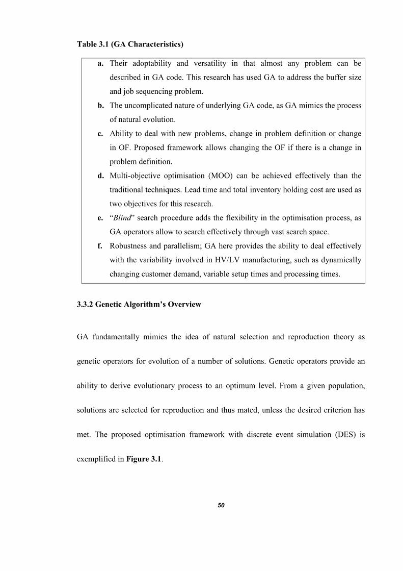
50

Table 3.1 (GA Characteristics)

a. Their adoptability and versatility in that almost any problem can be

described in GA code. This research has used GA to address the buffer size

and job sequencing problem.

b. The uncomplicated nature of underlying GA code, as GA mimics the process

of natural evolution.

c. Ability to deal with new problems, change in problem definition or change

in OF. Proposed framework allows changing the OF if there is a change in

problem definition.

d. Multi-objective optimisation (MOO) can be achieved effectively than the

traditional techniques. Lead time and total inventory holding cost are used as

two objectives for this research.

e. “Blind” search procedure adds the flexibility in the optimisation process, as

GA operators allow to search effectively through vast search space.

f. Robustness and parallelism; GA here provides the ability to deal effectively

with the variability involved in HV/LV manufacturing, such as dynamically

changing customer demand, variable setup times and processing times.

3.3.2 Genetic Algorithm’s Overview

GA fundamentally mimics the idea of natural selection and reproduction theory as

genetic operators for evolution of a number of solutions. Genetic operators provide an

ability to derive evolutionary process to an optimum level. From a given population,

solutions are selected for reproduction and thus mated, unless the desired criterion has

met. The proposed optimisation framework with discrete event simulation (DES) is

exemplified in Figure 3.1.

51

Figure 3.1 (Proposed Combinatorial Optimisation Model)

3.3.2.1 String Encoding and Objective Function

The GA process starts with the initial population of solutions. Each individual in

population represents a solution to the problem, called “Chromosomes” or “Strings”.

Chromosomes are usually expressed as a string of variables; each element of

chromosome is known as “gene”. Chromosome representation is one of the vital factors

52

in GA as it stores problem specific information, which can affect performance and

outcome of the algorithm (Song and Hughes, 2002).

Proposed research methodology has used real number and binary encoding to represent

the job sequence and buffer size problem respectively i.e. problem representation is

based on two chromosomes. The size of chromosome representing buffer sizes (BS) and

job sequences (JS) depends on the number of buffers involved (p) in the system and

number of work types (q) respectively. Along this, evolution process takes place up to n

generations and each generation has m chromosomes (i.e. population size). The main

reason behind using two different type of chromosome is;

a. Binary representation of buffer sizes provides following advantages;

I. Smaller size of population is required even to represent large search

space, as search space can be managed by altering the binary values.

II. Makes genetic operations easier to operate across the large search space.

b. On the other hand, real number representation of job sequence provides easily

manageable relation between job type and quantity.

53

OF provides a mechanism to evaluate the performance/quality of each chromosome. OF

plays, an imperative role in the success of an optimisation process by describing calibre

of each chromosome towards the formulated objective. It is important to note that the

fitness of each chromosome is measured in terms of OF (Tang et. al., 2002).

In this research, two objectives have been used, which are reducing lead time and total

inventory holding cost.

3.3.2.2 Initialisation

Population in GA terminology represents the collection of chromosomes or set of

solutions. Before starting with any GA operation a set of chromosomes is needed i.e. the

subset of solution search space. Generating this subset of solutions is known as

initialisation, which is created randomly in most of the cases (Konak et al., 2006).

In current research, initial population (��) of generation (G) is generated randomly,

where population size m = 20. It is important to note that initial population contains two

types of chromosomes, i.e. to represent buffer sizes (binary chromosomes) and job

sequence (real number chromosomes), both can be represented as;

�� = ��, ��, ��, …… . ��, ��; �� = �� = �

54

3.3.2.3 Parent Selection

Selection method defines how to choose individuals in population that will create

offspring for next generation. Selection process can be affected because of following

factors (Song and Hughes, 2002);

a. Too strong selection halts evolution process by reducing diversity

b. Whereas, too weak selection will result in slow evolution.

Current research has adopted fitness-proportionate selection scheme by using concept of

Tombola. This can be described in following order (Table 3.2);

Table 3.2 (Selection Process)

a. Sort the population “��” of ith

generation (where i < n and n = 100)

according to fitness of individuals, which is derived from the two OFs; “LT”

and “TIHC”.

b. For m individuals generate “(�)(�+ �)/�” tickets and assign tickets

proportionally according to the fitness of each individual.

c. This biases the selection criteria and derives the evolution process towards the

fittest individuals. However, there is still a probability of worst chromosomes

to get selected, which is to;

I. Bring the randomness in the selection process

II. Maintain the diversity in population to prevent premature convergence and

stagnating of the evolution process.

55

3.3.2.4 Crossover

Once the parents have been selected then they are paired for matting. This mating

process is known as crossover, which is derived by crossover probability, typically

around 60% (Konak et al., 2006).

In this research, uniform cross-over has been used, where multiple crossover points are

defined on the basis of random number “r” generated for each selected individual. The

main reason of random uniform crossover is to increase the efficiency and effectiveness

of the algorithm by creating randomness.

3.3.2.5 Mutation

Mutation is an effective and powerful process that entails the random alteration of

gene/genes in selected chromosomes, typically carried out with a very low probability.

The main motive behind mutation is to maintain the diversity within population for

prevention of premature convergence of an algorithm to false peak and stagnation of the

evolution process. Along this, it can increase the diversity of chromosomes to exploit

the solution space (Hu and Paolo, 2007).

In this research, uniform mutation has been used for the job sequence and multi-point

flip bit for the buffer sizes, where multiple mutation points are defined on the basis of

56

random number “r” generated for each selected individual. The main reason of random

uniform mutation is to preserve the original relation between the part number and

quantity. Along this, multipoint mutation increases the efficiency and effectiveness of

the algorithm by allowing to search in wider solution space.

3.3.2.6 Inversion

Inversion defines the concept of rearrangement of chromosome in which either a

segment or whole chromosome is reversed end to end to produce a new child (Chunhua,

2010). This research has used inversion to invert the entire chromosome.

3.3.2.7 Replacement Strategy

Once new population has generated, old population needs to be replaced with new

generation. Current research has adopted generational replacement with elite strategy.

This can be described in Table 3.3;

Note: Elitism force GA to retain some number of individuals, which are copied as such

to next generation without any changes. This may increase the speed of domination of a

super chromosome Tang et al. (2002).

57

Table 3.3 (Replacement Strategy)

a. Generate new population of size “m”, which is equal to the size of old

population; where m = 20.

b. Use elite strategy by keeping “e” best individuals from old generation, where

1 ≤ e ≤ k. Where value of “k” (typical value of “k” is 1 or 2. This can also

derived from the number of objective) must be kept low to maintain

evolution process. In this research, the value of “k” is derived from the

number of OFs i.e. k = 2.

c. Replace “m - k” individuals of old generation with new population.

3.3.2.8 Evaluation

Once the population has been copied to the new generation, it needs to be evaluated

again to check the fitness of new solutions i.e. calculate the fitness of each chromosome

in terms of OF i.e. lead time and total inventory holding cost. In this research, DES tool

(Simul8) has been integrated with the proposed multi-objective GA framework to

validate the fitness of each individual in the current generation.

3.3.3 Multi-Objective Combinatorial Optimisation

According to Konak et al. (2006), “combinatorial optimization is a topic in theoretical

computer science and applied mathematics that consists of finding the least-cost

solution to a mathematical problem in which each solution is associated with a

numerical cost”.

58

Many manufacturing optimisation problems are multi-objective, having been conflicting

with objectives and system constraints, where optimising the single objective can result

in unacceptable results with respect to other objectives. Therefore, the prime motive of

an optimisation is to investigate a set of solutions to satisfy objectives to an acceptable

level without being dominated by any other solution. Multi-objective combinatorial

optimisation here not only relates the objective to a numerical cost but also defines

more than one objective for optimisation (Tamaki et al., 1996; Konak et al., 2006 and

Deb et al., 2002).

Researchers have proposed different optimisation approaches, but applicability of these

approaches in different problem areas is subjected to constraints imposed by the

problem. For instance, too many variables in problem make the optimisation process

harder, as the complexity of interrelationship between these variables makes sometimes

accurate modelling almost impossible. Additionally, existing solution techniques are

often limited by involvement of many qualitative variables (Stockton et al., 2004). Most

of the proposed approaches in optimisation literature are single objective, which are

incapable of dealing with the complexity of the real-world problems, as optimising the

single objective may deteriorate the performance of other organisational objectives. For

59

instance, increasing the input rate of product to the system generally increases the

throughput, but it also increases the WIP (Cochran et al., 2003).

Current research has opted GA based multi-objective combinatorial Optimisation

approach to determine the optimal buffer size and job sequence. Multi-Objective

optimisation has been chosen because of complexity of problems in manufacturing

system and high product variability in flow lines.The main focus of research is to

optimise the job sequence and buffer sizes based on the organisational objectives, which

are lead time and total inventory holding cost by maintaining the system constraints.

Multi-objective combinatorial optimisation elaborates the concept of finding all the

trade-offs between multiple OFs, which are usually conflicting one’s. Along this, GA

provides the advantage over the traditional optimisation approaches such as

mathematical modelling, which are (Xia and Wu, 2005);

a. Reduced computational complexity.

b. Ability to combine the several optimisation criteria and to deal with complex

real-world problems effectively.

60

3.3.3.1 Existing Multi-Objective Optimisation Approaches

There are numerous applications of multi-objective combinatorial optimisation in

different manufacturing process problems. For instance;

Xia and Wu (2005) have applied multi objective swarm optimisation for flexible job-

shop scheduling problem (FJSP) to minimise the makespan and total workload of

machines. Proposed FJSP consist of two sub problems, which are routing and

scheduling sub-problem. Routing sub-problem allows assigning an operation to a

machine from the set of capable machines and scheduling sub-problem minimises the

predefined OF by generating a feasible schedule out of assigned operations. However,

proposed approach doesn’t guarantee to provide an optimal solution, the main motive to

find good-quality solution within a reasonable time (Xia and Wu, 2005).

On the other hand, Cochran et al. (2003) has exemplified the application of multi-

objective GA to solve the scheduling problem for parallel machines, where OF is

minimising the makespan, total weighted completion time and total weighted tardiness.

In order to get the optimal schedule system constraints are maintained, such as; release

times, process times, setup times and due dates. Here proposed algorithm produces too

many unwanted solutions for each objective is evolved separated in sub-populations,

61

which are later combined using weighted sum approach. Along this, it increases

complexity and time for conversion as the number of objectives increased.

Similarly, Jamshidi et al. (2011) has used a multi-objective GA for planning order

release dates for a two-level assembly line to minimise the holding cost and

backlogging cost by using the system constraints as known demand and due dates for

finished product. Again, in the scheduling framework, Ko and Wang (2011) have

applied GA in production scheduling problem to achieve a better trade-off between on-

time delivery, shorter LTs and maximum resource utilisation, where resources and

buffer sizes are considered as constraints. It has been noticed that, as the buffer size

increases the penalty cost increases, which also creates unrealistic schedules. In

proposed approach, buffer sizes are derived from the experimental data, which may not

be valid when system condition changes such as product sequence and resources.

Mansouri (2005) has applied GA based multi-objective optimisation for a job

sequencing in JIT mixed-model assembly lines to reduce the variation of production

rates and number of setups simultaneously due to diversified customer demand. Two

objectives here are conversely related to each other. Proposed research model has used

the elite preserve strategy to retain the best solution from each generation and

62

optimisation process is derived on the basis of production rate variation, number of

setups, number of unique products and total number of units.

Solimanpur et al. (2004) have integrated mathematical model and GA based multi-

objective optimisation to find the optimal cells in order to reduce the LT and cost.

However, using mathematical model, researchers have shown inability to capture all the

complexity of real-world problems. Similarly, Filho and Tiberti (2006) have used GA

for cell layout design, where weighted sum approach has been used to combine the

multiple objectives (i.e. inter cell flow and WIP) to single objective. However, it has

been noticed that as the size of the problem increases the efficiency of the algorithm

decreases i.e. it needs more time for convergence.

In multi-objective optimisation framework, Yang et al. (2012) have exemplified the

application of GA in mixed-model assembly line rebalancing to respond to changing

customer demand in order to reduce the level of variability in the production

environment. The optimisation criterion is based on minimising the number of stations,

workload variation at each station and rebalancing cost. Similarly, Ponnambalam et al.

(2003) have applied multi-objective GA to get the optimal sequences in the mixed

model assembly lines. Proposed approach here has considered three main objectives,

which are minimising the variability in part usage, total setup time and total utility

63

work. Utility work here defines the utility workers required to assist regular workers

during the work load. Proposed model has considered the part usage as a main

constraint at the different level of assembly (for instance, at raw material, product, sub

assembly and component level). However, other types of variability are not considered

such as machine failure or changing customer demand.

In combinatorial optimisation literature, there are other methods used as well, for

instance ant colony mechanism, swarm optimisation, mathematical modelling and water

flow optimisation algorithm. However, GA has always dominated all other techniques

in terms of their applicability in a wide range of problems.

It is important to note the comparison between different optimisation techniques is not

in the scope of this research.

3.3.3.2 Proposed Combinatorial Optimisation Framework

In this research, proposed combinatorial optimisation framework has used the concept

of Pareto optimality with elite preserve strategy. Two dominant solutions are saved in to

the final set of solutions from each generation i.e. one dominant solution with respect to

each OF, which is lead time and total inventory holding cost. This provides a set of

64

optimal solutions for decision makers according the trade-off between lead time and


Along this, in the evolution process chromosome selection (for crossover, mutation and

inversion) is based on the random weighted sum approach to simplify the two

objectives, where random weights are generated for each chromosome to maintain the

population diversity. Also, random weights provide advantages over fixed weights by

not generating the solutions, which are biased according to the assigned weights.

3.4 Performance Measure (PM)

PMs provide basic building block for PI by giving timely feedback of organisational

elements. Researchers have regarded PMs as a foundation for organisational

achievements (Folan and Browne, 2005). Similarly, Lohman et al. (2004) have regarded

PMs as an essential prerequisite for PI, which includes financial and non-financial

measures for process monitoring. The basic idea behind using PMs is to improve overall

organisation’s operational performance.

According to Lohman et al. (2004) “PM is an activity that managers perform in order

to reach predefined goals that can be derived from company’s predefined strategic

65

objectives”. Whereas, Nelly et al. (1996) have defined PM as “a metric used to quantify

the efficiency and/or effectiveness of action”.

PMs play an important role in process improvement to (Folan and Browne, 2005);

a. Measure progress against organisational goals

b. Identify improvement opportunities

c. Quantify and evaluate performance against internal and external standards.

Lean philosophy has successfully implemented and proved using PMs in the area of PI.

This research has opted operational level PMs by comparing and altering output and

input values respectively according to predefined goals. Here, the discrepancy between

the actual and expected value of selected performance measures that can assist the

process of CI by emphasising possible problem areas. However, researchers have

emphasised on the selection of an appropriate PM, as it plays the critical role in success

of organisation. Selection of wrong PM can be a major barrier to success of organisation

by obstructing and misleading the CI process. Table 3.4 illustrates the characteristics of

effective PMs (Folan and Browne (2005), Lohman et al. (2004), Nelly et al. (1996),

Nelly et al. (2000) and Gunasekaran et al. (2001));

66

Table 3.4 (Characteristics of Performance Measures)

a. Selected PMs should consistently contribute towards the organisational goals

such as enhanced effectiveness and competitiveness, better customer care

and increased profitability. This also includes commitment of people

involved at different organisational levels to prevent any miscommunication.

b. PMs should reflect the organisation’s strategy, aims, objectives and

operations to avoid any ambiguity in PI, i.e. PMs should be able to measure

the gap between the actual and expected outcome without any conflict with

other measures.

c. PMs should quantify efficiency and effectiveness of operations based on the

characteristics of organisation’s operations and should be reflected in the

definition of used PMs.

d. PMs should fully liaise with process functionality, i.e. identification of

primary data source and collection method to evaluate and improve

candidate organisational goal.

e. PMs should provide simple, reliable, visible and easily quantifiable

information in order to regulate decision-makers to monitor, control and

improve the candidate problem.

f. PMs should enable problem solver and decision-makers to monitor

performance of several areas simultaneously by identification of different

factors, variables and their interrelationships.

3.5 Summary

This chapter has exemplified the concept of RCA and GA based combinatorial

optimisation to automate the operational performance in context of lean CPS. Research

here has investigated the job sequence and buffer size optimisation to reduce lead time

and total inventory holding cost while maintaining the other system constraints, such as

67

variable processing times, variable setup times, machine failure, product dependent

routings and variable customer demand. The main focus remains here to inherit some of

the core components of lean philosophy, i.e. response to variable customer demand and

reduce the effect of variability to improve synchronous flow by considering the effect of

performance improvement of different PM’s on each other.

68

Chapter 4 – Research Methodology

4.1 Introduction

This chapter illustrates the steps undertaken to build the research methodology. The aim

of this research is to develop a novel method to automate operations in process

improvement (PI). To achieve this aim research here has exploited the concept of drum-

buffer-rope (DBR) to promote the synchronous flow by minimising the level of

variability in high variety and low volume (HV/LV) manufacturing environment. The

proposed method will allow problem solvers and decision-makers to determine the

optimal buffer sizes and job sequence under the operational constraints to reduce the

level of variability. In this research, the effect of variability is measured based on the

fitness functions for combinatorial optimisation model i.e. lead time (LT) and total

inventory holding cost (TIHC). As discussed in chapter 2, there are different

operational constraints that can affect task/process synchronisation as a result of the

different types of variability that can occur in flow production, e.g. high product variety,

low volume, routings and variable customer demand, processing times and setup times.

To achieve this, a multi-objective genetic algorithm (GA) based combinatorial

optimisation model has been proposed to reduce the effect of variability according to

69

selected performance measures (PM). Along this, proposed methodology is integrated

with “Discrete Event Simulation (DES)” model in order to respond to the rapid

changes in customer demand and product mixes.

To achieve research aim, following objectives need to be considered to produce a

comprehensive description of requirements and for practical implementation of a

proposed framework to overcome the manufacturing problems (Section 2.4);

a. Quick response to the mixed level of variability that may affect the order

fulfilment or flow line’s efficiency such as changes in customer demand, product

mix, routings, breakdowns (breakdowns represent long stoppages) and

measuring their effect on different performance measures such as lead time and


b. Task synchronisation within a flow line by identifying bottleneck, i.e. DBR

system.

c. Use of different combinatorial objective functions (OF) to determine the solution

fitness, for instance, lead time and total inventory holding cost.

d. Using GA based combinatorial optimisation and DES tool as an iterative method

for buffer management and controlling job sequencing.

70

e. Considering the effect of improvement of different performance measures (PM)

on each other under optimisation process.

4.2 Research Methodologies Overview

Research methodology is a philosophy that enables researchers to examine critically

various aspects of professional work.

According to Davy and Valecillos (2009) research methodology can be defined as “The

systematic collection and analysis of observations for the purpose of creating new

knowledge that can inform actions and decisions”.

Researchers have regarded it as a philosophy that guides the research towards defined

aims and objectives. Research methodologies can be divided into three categories,

which are “Quantitative”, “Qualitative” and “Triangulation” (Creswell, 2003; and Yin,

2009).

4.2.1 Quantitative Research

Quantitative research is a method to fragment and define phenomena into measureable

groups. The main application of quantitative research is in social and natural sciences

e.g. physics, biology and sociology. In quantitative research evidences are evaluated and

71

refined using an iterative process using mathematical models, theories and hypothesis

for a specific problem domain. In other words, findings are entirely based on analysis of

statistical data i.e. variables and their interrelationships are the fundamental of the

quantitative research. Quantitative research focus is objective rather than subjective

(Davy and Valecillos, 2009). Similarly, according to Will et al. (2002), quantitative

research is a rational knowledge generation approach based on quantitative and causal

relationship between the problem domain specific variables. It is assumed that, the real

life problems and system behaviour can be captured by using an objective/conceptual

model.

Quantitative methodology consists of following steps (Khalil, 2005);

a. Data collection; techniques are surveys and experiments. Random and specific

data samples can be collected on the basis of conditioned and quasi experiment

techniques respectively.

b. Data examination; using mathematical model or hypothesis.

c. Defining relationships by statistical analysis.

d. Finally visualisation of results in the form of tables or charts.

72

Quantitative research can be carried out into three different ways; “Experimental

Techniques”, “Quasi-experimental Techniques” and “Survey Techniques” (Robson,

2006).

4.2.2 Qualitative Research

Qualitative methodology represents a subjective approach rather than objective; based

on detailed description of given problem, procedure, observed behaviour and/or general

opinion. According to researchers, qualitative methods are associated with traditional or

scientific research mainly through interview, focus group, case study, direct observation

and survey. Hence, it needs understanding and co-operation between researchers and

participants to keep context trustworthy and unambiguous as there is always some

degree of presumption by the researcher and inception by the participant (Graneheim

and Lundman, 2004). However, Davy and Valecillos (2009) have described qualitative

methodology more challenging and time-consuming than quantitative.

According to Creswell (2003) “qualitative approach is one in which the inquirer often

makes knowledge claim based primarily on constructivist perspective”.

73

In contrast to quantitative methodology, qualitative methodology allows a researcher to

work with small and focused samples instead of random samples. Qualitative

methodology includes following steps;

a. A data collection method includes content analysis, interviews, observation,

focus group and usability.

b. Detailed description of organisational trends, techniques, process, entities and

deliverables.

c. Analysis of focused information set to identify the problem.

4.2.3 Triangulation

Triangulation is also known as the mixed methodology, which is a combination of both

qualitative and quantitative methodology. Using more than one methodology provides

the multidimensional insight to the research problems. Additionally, triangulation can

overcome the weakness and potential biases of the single methodological approach.

4.3 Research Methodology

This research has used the triangulation as research methodology, i.e. the mix of

qualitative and quantitative data. Initial data has been collected through literature review

and from the collaborator’s feedback as this research is part of a research project funded

74

by Technology Strategy Board (TSB) (Ref: K1532G). Therefore, proposed method

steps were based on data collected through meetings with collaborators beside the

literature review that was carried out. In addition, collaborators were involved in

validation of every step during the development of the proposed method.

The proposed research methodology includes two main components, which are discrete

event simulation (DES) and multi-objective combinatorial optimisation model, as given

in Section 4.3.1 and 4.3.2.

4.3.1 Discrete Event Simulation Model

The method developed within this research has used DES as a tool to represent the

investigated working areas. It acts as an iterative tool with combinatorial optimisation

model to find optimum job sequence and buffer sizes based on given system constraints.

Along this, enables the optimisation model to quantify and validate any job sequence

and buffer sizes during the evolution process. According to the literature review, the

research has summarised some of the benefits of using DES, which are (Banks, 1999;

Banks et al., 1996; and Sandanayake et al., 2008);

75

a. Investigating new operations, procedures, rules and flow. These can be

examined without interrupting and allocating resources in the real life as, post

implementation alterations are expensive and time consuming.

b. Allowing measuring the effect of the variability with respect to time based on

the selected performance measures. Along this, it allows systematic

investigation for problematic areas by controlling the simulation speed and

simulation run time.

c. Ability to illustrate simple to complex systems such as mixed type of flow, i.e.

subassemblies, parallel production and flow production. However, current

research has represented a flow line consist of five work stations.

d. Providing an opportunity to exploit system constraints and their effect on PMs

through the analysis of collected data. For instance, bottleneck analysis can be

performed with respect to Work-in-Progress (WIP) and excessive delays.

e. Observing and analysing the behaviour of the system helps to come with best

possible or optimal solution. In addition, these solutions can be tested before

implementation. For instance, current research has used DES with GA based

76

combinatorial optimisation methodology to find the optimal solution for buffer

management problem.

f. Can be used for training purpose, as decision inputs can be fed back to DES

model and results can be visualised to observe the system behaviour before and

after any changes.

4.3.2 Multi-Objective Combinatorial Optimisation Model

Current research has used multi-objective GA (Section 3.3) to develop combinatorial

optimisation methodology. There are numerous applications of GAs, where they have

been used widely to optimise and improve the performance of the manufacturing

systems (Section 3.3.3.1). Despite manufacturing, there are other various examples,

which exemplify the successful implementation of GAs in real-world problems. Current

research extends the existing optimisation concept to the combinatorial optimisation

that will not only look at providing optimum solution but also the possibility of;

a. integrating combinatorial optimisation with DES model,

b. being a part of lean creative problem solving,

c. investigating the effect of different PM’s improvement on each other, and

d. Developing a buffer management system for task synchronisation.

77

4.4 Proposed Research Framework: Research steps can be given as Figure 4.1:

Figure 4.1 (Proposed Research Framework)

78

Step 1 - Data Collection: initial data needs to be collected for the development of DES

model to represent a real environment, which will be collected from the different

collaborators who are part of the Technology Strategy Board Project ref: K1532G.

DES model represents a flow line of “Five WorkCentre” that are representing a

working area having several system constraints (Step 2).

Step 2 - Develop Simulation Model: Current DES model represents a working area at

Perkins where different type of variability is induced within the model, for example,

variable cycle time, buffer sizes, queuing time, dynamic customer demand, product mix,

routing and breakdowns. Table 4.1 gives an overview of the modelling elements

included in DES model.

Table 4.1 (Simulation Parameters)

Simulation Parameters Value

Simulation Run Time Determined based on customer order, i.e. quantity

ordered by a customer.

Travel Time It was set to Zero, to avoid the effect of any hidden

type of variability that can affect end of simulation

runs results.

Random Time No randomness has been included as model represents

a real working area.

Shift Pattern No shift pattern has been included.

79

Probability Distribution Triangular distribution has been chosen as it provides

an acceptable trade-off between the accuracy of results

and estimation of distribution parameters (Khalil et al.

2010).

Resources Not been identified, as proposed methodology is

looking at the manufacturing process.

It is important to note that the values for triangular distribution are derived by

estimating activity’s absolute minimum, most likely and maximum time values.

Step 3 - Identify Modelling Element (ME) Attributes: Table 4.2 exemplifies the ME,

as used in the DES model. As the model is integrated with the GA based combinatorial

optimisation code, therefore, generic names were given to different WorkCentre within

a working area, i.e. M1 which represents the first WorkCentre on the production line

and so on.

Table 4.2 (Simulation Modelling Element Attributes)

Modelling

Elements

Type Attribute Value

Queue for M1

Queue for M2

Queue for M3

Queue for M4

Queue for M5

Queue Capacity (Number) Infinite; before optimisation no

restriction has been imposed on

queue sizes. However, queue sizes

are derived during the optimisation

process by considering the system

constrains such as batch size.

However, user can have initial

queue capacities if required because

of model change.

M1

M2

WorkCentre Cycle Time (Min) Differ according to the product type,

as exemplified in Table 4.4.

80

M3

M4

M5

Setup Time (Min) Differ according to the product type,

as exemplified in Table 4.4.

Batch Sizes 1, 5, 10

Queue for M1 Queue Inventory Holding Cost £ 0.2 per unit per minute





M1 WorkCentre Machine Failure MTTF (min) = 75,85,95

MTTR (min) = 5,15,25


MTTR (min) = 10,15,20


MTTR (min) = 10,20,30


MTTR (min) = 0,10,20


MTTR (min) = 10,15,20

Step 4 – Generate Different Customer Demand: Customer demand has been taken as

an input to the DES and combinatorial optimisation model to evaluate the proposed

research methodology. Customer demand represents the product type and quantity to be

produced, which can be given as;

a. Product Quantity; variability in terms of different product types, which may

have different or same quantity to be produced as shown in Table 4.3, where

Work Type represents Part Type i.e. different items needs to be produced may

be with different or same quantities. Experiments have been carried out with ten

81

different work types having 500, 1000 and 2000 items to produce in total

quantity, i.e. customer demand.

Table 4.3 (Product Quantity with Different Work Types)

Work Type Quantity (Number of Parts)

1 60 100 100

2 50 200 250

3 30 150 50

4 40 100 200

5 60 100 100

6 50 60 350

7 80 100 300

8 50 40 250

9 60 100 300

10 20 50 100

Total Quantity 500 Parts 1000 Parts 2000 Parts

b. Product Mix; similarly, variability may exist in terms of cycle time, setup time

and route followed by the particular product as exemplified in Table 4.4.

Table 4.4 (Product Mix with Different Routings)

Work Type Job Location Timing (min) Changeover (min)

1 1 M 1 5 0

1 2 M 2 8 30

1 3 M 3 2 10

1 4 M 4 3 0

1 5 M 5 5 20

1 6 Exit 0 0

2 1 M 2 10 70

2 2 M 3 5 10

2 3 M 4 5 0

2 4 Exit 0 0

82

3 1 M 1 7 0

3 2 M 2 15 30

3 3 M 4 3 15

3 4 M 5 3 15

3 5 Exit 0 0

4 1 M 1 8 0

4 2 M 2 30 30

4 3 M 3 4 10

4 4 M 4 5 25

4 5 M 5 3 20

4 6 Exit 0 0

5 1 M 1 6 0

5 2 M 2 10 45

5 3 M 3 9 15

5 4 M 5 4 25

5 5 Exit 0 0

6 1 M 1 5 0

6 2 M 2 15 45

6 3 M 4 2 0

6 4 M 5 3 20

6 5 Exit 0 0

7 1 M 2 15 55

7 2 M 3 3 7

7 3 M 4 2 0

7 4 M 5 2 15

7 5 Exit 0 0

8 1 M 2 8 35

8 2 M 3 3 7

8 3 M 4 2 0

8 4 M 5 2 20

8 5 Exit 0 0

9 1 M 1 5 0

9 2 M 2 12 50

9 3 M 3 3 25

9 4 M 4 4 0

9 5 M 5 5 25

9 6 Exit 0 0

83

10 1 M 2 2 95

10 2 M 3 8 0

10 3 M 5 2 20

10 4 Exit 0 0

It is important to note that terminology used in Table 4.3 and Table 4.4 is from simul8

where;

a. Work Type represents the different part type.

b. Job is the route followed by each part.

c. Location is the work centre where job has been processed.

d. Timing represents the processing time and Changeover represents the setup

time when there is change in the product type.

Step 5 – Identify Performance Measures (PM): According to Blackstone and Jonah

(2008) performance measure can be defined as “a system for collecting, measuring, and

comparing a measure to a standard for a specific criterion for an operation, item/good,

service and business.” As discussed in Section 3.4 PMs are one of the essential

components to address organisational problems, performance gap and other anomalies.

In current research, PMs are used as a part of measuring the different type of variability

quantitatively for analysis and visualisation of results as well as to evaluate the

performance of proposed methodology. Table 4.5 exemplifies the PMs used in current

84

research. Here, lead time and total inventory holding cost are used as the fitness

measure for the combinatorial optimisation method. As exemplified in Table 4.5, other

performance measures are the contributing factor towards the lead time and total

inventory holding cost. Furthermore, these measures are used for initial result’s

analysis.

Table 4.5 (Selected Performance Measures)

Performance Measure Unit of Measurement

1. % Waiting Percentage

2. % Blocking Percentage

3. % Stopped Percentage

4. % Working Percentage

5. % Change Over Percentage

6. Average Queue Size No of Parts

7. Average Queuing Time Minutes

8. Work in Progress No of Parts

9. Total Inventory Holding Cost £ per Part Per Minute

10. Lead Time Minutes

Step 6 – Bottleneck Identification

According to Blackstone and Jonah (2008), bottleneck is “A resource whose capacity is

less than the demand placed upon it”. For example, a WorkCentre is said to be

bottleneck if jobs are processed at the slower rate than demand. In this research,

correlation analysis is used to identify the bottleneck by analysing the lead time and

85

total inventory holding cost against other PM’s, i.e. average queue size, average

queuing time, % waiting, % working and % changeover. This will allow determining

the effect of each modelling element on lead time and total inventory holding cost

according to selected PMs.

According to Fresco (2010), A WorkCentre is said to be bottleneck if WorkCentre is

having;

a. Largest processing queue sizes. Current research has investigated the effect of

average queue size for each WorkCentre on lead time and total inventory

holding cost.

b. Longest waiting time. Investigating the effect of average queuing time for each

WorkCentre on lead time and total inventory holding cost.

c. High level of variability, which can be determined from % waiting, % working,

% changeover and % stopped.

d. Jobs with highest capacity requirements.

e. Higher inter-arrival time than processing capacity.

Note: It is important to note that bottleneck identification, here is only used to

demonstrate that as manufacturing environment complexity and variability increases

86

traditional approaches are not competent enough identifying the bottleneck process. In

the HV/LV manufacturing environment bottleneck identification is difficult as it can

shift with the different product mixes and stochastic features of manufacturing systems.

Current research has proposed combinatorial optimisation model to achieve

synchronous flow in complex and dynamic manufacturing environment, which is

exemplified in step 7.

Step 7 – Development of Drum-Buffer-Rope (DBR) Optimisation Rules:

Research here has developed GA based combinatorial optimisation rules for DBR

implementation. Proposed GA based rules have investigated the cause of variability on

individual WorkCentre but fitness of each solution is measured against the lead time

and total inventory holding cost, i.e. overall system performance.

For proposed model results are collected according to;

a. Firstly, buffer size optimisation

b. Secondly, job sequence optimisation and

c. Finally, Buffer size and job sequence optimisation

The optimisation rules can be given as in Table 4.6.

87

Table 4.6 (Combinatorial Optimisation Rules)

Variables Fitness Function Objective

Buffer Sizes Lead Time and Total

Inventory Holding Cost

Determining the optimal buffer sizes

Job Sequence Lead Time and Total


Determining the optimal job sequence

Buffer Size and Job

Sequence

Lead Time and Total


DBR implementation to achieve process

synchronisation

Step 8 – Carry More Experiments and Continuous Improvement: Carry more

experiments until customer demand has met by introducing the different level of

variability. For example, machine breakdowns, routings and setup times. This will

further allow reducing the effect of different type of variability form the flow line. As,

product mix changes there may be different routings, setup times and process times.

Here, proposed research framework has inbuilt capability to address the

interrelationship between the different performance measure, which allows to optimise

the buffer sizes without knocking out any other performance measure.

88

Chapter 5 – Experimental Results

5.1 Introduction

This chapter exhibits the experimental result on the basis of data collected through the

methodology developed in the Chapter 4. The aim and objectives of research have been

achieved by implementing the research methodology steps as described in Chapter 4.

Initial and post optimisation results are collected by including different level of

variability such as customer demand, product mix, processing times, setup times,

machine failures and routings. All the results are presented with respect to the fitness

functions used for optimisation, i.e. lead time (LT) and total inventory holding cost

(TIHC).

Initial experiments are carried out to identify the constraint resource or problem in the

flow line and correlation analysis is used to demonstrate the complexity of

interrelationships between different modelling elements. Along this, combinatorial

optimisation has been applied to determine the optimal buffer size and job sequence to

reduce the effect of variability and to elevate the constrained resource. Proposed

combinatorial optimisation has shown a significant improvement in the investigated

performance measure, as discussed further in this chapter.

89

5.2 Experimental Results

Step 1 – 5: research here has used both qualitative and quantitative techniques for data

collection, as discussed in Section 4.4. In this research, discrete event simulation (DES)

model is developed based on the data collected, which represents a working area of

Perkins based on the parameters described in Table 4.1.

Initial results are collected according to the different types of variability, i.e.

a. Machine failure, batch size and inventory holding cost per unit as shown in

Table 4.2.

b. Customer demand in terms of product quantity and type, which is described in

Table 4.3.

c. Processing time, setup time and routing i.e. flow of material Table 4.4.

Collected results are shown according to the performance measures described in Table

4.5, which can be given as;

a. Table 5.1a exemplifies the average queuing time and average queue size,

whereas Table 5.1b demonstrates the % Working, % Waiting, % Changeover

and % Stopped for the 500 parts.

90

b. Similarly, Table 5.2a illustrates the average queuing time and average queue

size, whereas Table 5.2b demonstrates the % Working, % Waiting, %

Changeover and % Stopped for the 1000 parts.

c. Finally, Table 5.3a represents the average queuing time and average queue size,

whereas Table 5.3b demonstrates the % Working, % Waiting, % Changeover

and % Stopped for the 2000 parts.

Note: It is important to note that % Blocking is not used in initial analysis; i.e. initial

buffers are used as infinite size, as optimal buffer sizes will be investigated later through

combinatorial optimisation.

91

a. 500 Parts; Table 5.1a represents the average queuing time and average queue size for different batch sizes i.e. batch size 1, 5 and

10.

Table 5.1a (Average Queuing Time and Average Queue Size for 500 Jobs and Batch Size 1, 5 and 10)

Exp. N

o.

Batch

Size

Mach

ine F

ailu

re

Total In

ven

tory H

olding

Cost

Lead Tim

e

Average Queuing Time (min) Average Queue Size (number)

Queu

e for M

1

Queu

e for M

2

Queu

e for M

3

Queu

e for M

4

Queu

e for M

5

Queu

e for M

1

Queu

e for M

2

Queu

e for M

3

Queu

e for M

4

Queu

e for M

5

1 1 No 1,562,810 16,749 166 6,210 0.59 0.04 1.46 3 185 0 0 0

2 1 yes 2,032,863 20,489 268 8,062 3.12 1.85 4.07 4 197 0 0 0

3 5 No 1,159,705 9,386 717 4,464 1.36 0.04 1.63 23 238 0 0 0

4 5 yes 1,311,448 10,742 862 5,032 4.44 2.23 3.79 24 243 0 0 0

5 10 No 925,438 7,966 806 3,505 1.99 0.09 2.39 30 220 0 0 0

6 10 yes 1,084,242 9,287 951 4,101 5.5 2.01 3.75 31 220 0 0 0

92

Table 5.1b illustrates % working, % waiting, % changeover and % stopped for different batch sizes i.e. batch size 1, 5 and 10.

Table 5.1b (% Working, % Waiting, % Changeover and % Stopped for 500 Jobs and Batch Size 1, 5 and 10)

Batch

Size

Mach

ine F

ailu

re

% Working % Waiting % Changeover % Stopped

M1

M2

M3

M4

M5

M1

M2

M3

M4

M5

M1

M2

M3

M4

M5

M1

M2

M3

M4

M5

1 No 10.4 37.8 10.7 7.9 8.9 89.6 0.3 82.1 91.9 69.4 0 61.8 7.1 0.2 21.6 0 0 0 0 0

1 yes 8.5 30.9 8.8 6.4 7.3 76.7 0.1 62.2 75.4 59 0 54.1 8.9 0.2 18.9 14.8 14.8 20.1 18 14.8

5 No 18.5 67.5 19.2 14.1 16 81.5 0.2 75.9 84.6 74.5 0 32.2 4.9 1.4 9.5 0 0 0 0 0

5 yes 16.2 59.1 16.7 12.3 13.9 68.8 0.2 59.2 69.1 62.6 0 26.2 4.6 0.6 8.7 15 14.6 19.5 17.9 14.6

10 No 21.8 79.6 22.6 16.6 18.8 78.2 0.3 73.4 82.9 73.7 0 20.1 4 0.5 7.4 0 0 0 0 0

10 yes 18.7 68.3 19.4 14.2 16.2 66.3 0.2 58.1 67.5 63 0 16.9 3.3 0.4 6.4 14.8 14.7 19.2 17.8 14.5

93

b. 1000 Parts; Table 5.2a represents the average queuing time and average queue size for different batch sizes i.e. batch size 1, 5 and 10.


Exp. N

o.

Batch

Size

Mach

ine F

ailu

re

Total In

ven

tory H

olding

Cost

Lead Tim

e


Queu

e for M

1

Queu

e for M

2

Queu

e for M

3

Queu

e for M

4

Queu

e for M

5

Queu

e for M

1

Queu

e for M

2

Queu

e for M

3

Queu

e for M

4

Queu

e for M

5

7 1 No 4,739,097 28,246 531 9,347 0.31 0.02 1.36 11 331 0 0 0

8 1 yes 5,849,511 29,744 782 11,502 3.74 2.62 4.54 16 387 0 0 0

9 5 No 4,100,013 18,756 3,985 7,225 1.71 0.02 0.96 129 385 0 0 0

10 5 yes 4,530,910 20,912 4,472 7,962 7.91 2.31 2.67 130 381 0 0 0

11 10 No 3,770,431 16,396 1,717 7,118 0.15 0.05 1.55 63 434 0 0 0

12 10 yes 4,290,147 18,898 2,039 8,073 8.84 2.51 3.72 65 427 0 0 0

94



Batch

Size

Mach

ine F

ailu

re


M1

M2

M3

M4

M5

M1

M2

M3

M4

M5

M1

M2

M3

M4

M5

M1

M2

M3

M4

M5

1 No 13.3 46.3 12.8 10.8 9.6 86.7 0.1 78.9 86.5 72.3 0 53.6 8.3 2.7 18.1 0 0 0 0 0

1 yes 12.6 43.9 12.2 10.3 9.1 72.7 0.1 60.4 66.4 63.4 0 41.1 7.2 5.2 12.6 14.7 14.8 20.2 18.1 14.9

5 No 20 69.7 19.3 16.3 14.5 80 0.1 76.9 82.2 80.9 0 30.2 3.9 1.5 4.6 0 0 0 0 0

5 yes 17.9 62.3 17.3 14.5 12.9 67.3 0.1 59.5 66.3 68.8 0 22.9 3.1 1.1 3.5 14.8 14.7 20.1 18.1 14.8

10 No 22.9 79.7 22.1 18.6 16.5 77.1 0.1 74.1 81.1 79.3 0 20.2 3.8 0.2 4.2 0 0 0 0 0

10 yes 19.8 69.5 19.1 16.1 14.3 65.3 0.1 57.7 65.6 67.2 0 15.9 3.1 0.2 3.6 14.8 14.8 20.1 18.1 14.8

95

c. 2000 Parts; Table 5.3a represents the average queuing time and average queue size for different batch sizes i.e. batch size 1, 5 and

10.


Exp. N

o.

Batch

Size

Mach

ine F

ailu

re

Total In

ven

tory

Holding Cost

Lead Tim

e


Queu

e for M

1

Queu

e for M

2

Queu

e for M

3

Queu

e for M

4

Queu

e for M

5

Queu

e for M

1

Queu

e for M

2

Queu

e for M

3

Queu

e for M

4

Queu

e for M

5

13 1 No 25,839,806 66,167 667 25,691 1.67 0.01 0.54 11 776 0 0 0

14 1 yes 33,980,772 85,304 975 33,761 3.51 2.28 2.71 12 791 0 0 0

15 5 No 18,315,468 41,348 9,259 16,269 8.21 2.45 3.71 246 787 0 0 0

16 5 yes 20,455,456 34,195 7,224 13,668 0.41 0.01 0.22 547 977 0 0 0

17 10 No 15,542,509 32,491 2,984 14,883 2.96 0.01 0.81 101 916 0 0 0

18 10 yes 17,800,888 37,446 3,547 17,004 16.33 2.45 6.55 104 908 0 0 0

96



Batch

Size

Mach

ine F

ailu

re


M1

M2

M3

M4

M5

M1

M2

M3

M4

M5

M1

M2

M3

M4

M5

M1

M2

M3

M4

M5

1 No 9.5 40.2 9.8 8.6 8.3 90.5 0.3 87.3 91.3 71.1 0 59.5 2.9 0.1 20.5 0 0 0 0 0

1 yes 7.4 31.2 7.6 6.7 6.4 77.8 0.1 68.9 75.3 58.8 0 53.9 3.4 0.1 19.7 14.8 14.9 20.1 18 15

5 No 35.8 59.2 21.2 24.8 9.5 64.1 0.1 70.7 75.1 90.4 0 40.7 8.1 0.1 0.1 0 0 0 0 0

5 yes 15.2 63.9 15.7 13.8 13.3 69.9 0.7 60.6 65.6 66.5 0 20.5 3.4 2.7 5.2 14.8 14.9 20.3 18 14.9

10 No 19.4 81.9 20.1 18.3 16.9 80.6 0.1 77.7 80.6 78.2 0 18.1 2.2 1 4.8 0 0 0 0 0

10 yes 16.8 71.1 17.4 15.2 14.7 68.4 0.1 60.1 66.4 65.5 0 14.1 2.2 0.5 4.9 14.7 14.8 20.3 17.8 14.8

97

Step 6: to identify the bottleneck, correlation analysis has been performed on the

collected results according to the rules described in the step 6 of Section 4.4.

a. Average Queuing Time; Figure 5.1a exemplifies the degree of correlation

between total inventory holding cost and average queuing time for different

batch sizes.

Figure 5.1a (Total Inventory Holding Cost vs. Average Queuing Time)

Similarly, from Figure 5.1b demonstrates the degree of correlation between lead

time and average queuing time for different batch sizes.

Figure 5.1b (Lead Time vs. Average Queuing Time)

-1.00

-0.50

0.00

0.50

1.00

Queue for M1 Queue for M2 Queue for M3 Queue for M4 Queue for M5

Total Inventory Holding Cost vs. Average Queuing Time

Batch Size 1 Batch Size 5 Batch Size 10

-1.00

-0.50

0.00

0.50

1.00


Lead Time vs. Average Queuing Time


98

b. Average Queue Size; Figure 5.2a, exemplifies the degree of correlation

between total inventory holding cost and average queue size for different batch

sizes.

Figure 5.2a (Total Inventory Holding Cost vs. Average Queue Size)

Similarly, Figure 5.2b, represents the degree of correlation between lead time

and average queue size for different batch sizes.

Figure 5.2b (Lead Time vs. Average Queue Size)

-1.00

-0.50

0.00

0.50

1.00


Total Inventory Holding Cost vs. Average Queuing Size


-1.00

-0.50

0.00

0.50

1.00


Lead Time vs. Average Queuing Size


99

c. % Working; Figure 5.3a, illustrates degree of correlation between total

inventory holding cost and % working for different number of parts.

Figure 5.3a (Total Inventory Holding Cost vs. %Working)

Similarly, Figure 5.3b, illustrates degree of correlation between lead time and %

working for different parts quantity.

Figure 5.3b (Lead Time vs. %Working)

-1.00

-0.50

0.00

0.50

1.00

M1 M2 M3 M4 M5

Total Inventory Holding Cost vs. %Working

500 Parts 1000 Parts 2000 Parts

-1

-0.5

0

0.5

1

M1 M2 M3 M4 M5

Lead Time vs. %Working


100

d. % Waiting: Figure 5.4a, illustrates degree of correlation between total

inventory holding cost and % waiting for different number of parts.

Figure 5.4a (Total Inventory Holding Cost vs. %Waiting)


waiting for different number of parts.

Figure 5.4b (Lead Time vs. %Waiting)

-1.00

-0.50

0.00

0.50

1.00

M1 M2 M3 M4 M5

Total Inventory Holding Cost vs. % Waiting


-1

-0.5

0

0.5

1

M1 M2 M3 M4 M5

Lead Time vs. % Waiting


101

e. % Changeover; Figure 5.5a, illustrates degree of correlation between total

inventory holding cost and % changeover for different number of parts.

Figure 5.5a (Total Inventory Holding Cost vs. % Changeover)


changeover for different number of parts.

Figure 5.5b (Lead Time vs. % Changeover)

-1.00

-0.50

0.00

0.50

1.00

M1 M2 M3 M4 M5

Total Inventory Holding Cost vs. % Changeover


-1

-0.5

0

0.5

1

M1 M2 M3 M4 M5

Lead Time vs. % Changeover


102

f. % Stopped; In current research % stopped refers to the long stoppages. There is

no direct relation between the % stopped and change in customer demand or

batch size. Machine failure is used as type of variability for data collection,

which drives % stopped in the final results. Along this, from Figure 5.6a and

Figure 5.6b, it is important to note that % stopped having weak positive

correlation between total inventory holding cost and lead time.

Figure 5.6a (Total Inventory Holding Cost vs. %Stopped)

Figure 5.6b (Lead Time vs. % Stopped)

-1.00

-0.50

0.00

0.50

1.00

M1 M2 M3 M4 M5

Total Inventory Holding Cost vs. % Stopped


-1

-0.5

0

0.5

1

M1 M2 M3 M4 M5

Lead Time vs. % Stopped


103

Step – 7: this segment describes the results after optimisation according to the variables

described in Table 4.6. Experiments have re-run again to collect the results after

optimisation, and are represented with respect to customer demand in terms of the total

number of parts. Along this, results from different runs are compared according to

different type of variability i.e. machine failure and batch sizes.

It is important to note that each combinatorial optimisation run represents two output

values. As elucidated in the Section 3.3.3.2, number of output values related to each

result is equal to the number of fitness functions, .i.e. from this research’s perspective

it’s lead time and total inventory holding cost.

Therefore, each experiment represents two dominant solutions, i.e. one with respect to

lead time and other with respect to total inventory holding cost and the selection of

solution from these dominant solutions is the choice of a decision-maker.

Note: it is important to note that this chapter only includes graphs for batch size 1.

Processed data for batch size 1, 5 and 10 is included in Appendix A1. Batch size 5 and

10 exhibits the similar trend as batch size 1.

NOTE: Figure 5.7 a – b, 5.8 a – b, 5.9 a – b, 5.10 a – b, 5.11 a – b and 5.12 a – b are

using logarithmic axis.

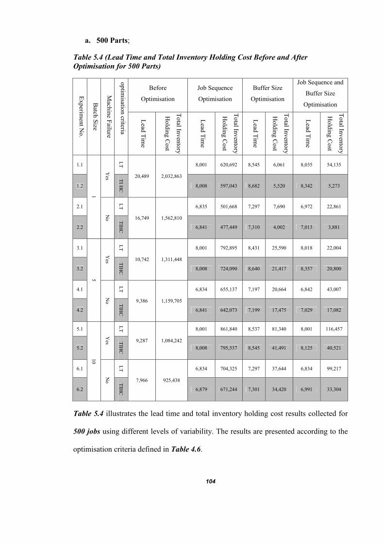
104

a. 500 Parts;

Table 5.4 (Lead Time and Total Inventory Holding Cost Before and After

Optimisation for 500 Parts)

Experim

ent N

o.

Batch

Size

Mach

ine F

ailure

optim

isation criteria

Before

Optimisation

Job Sequence

Optimisation

Buffer Size

Optimisation

Job Sequence and

Buffer Size

Optimisation

Lead

Tim

e

Total In

ven

tory

Hold

ing C

ost

Lead

Tim

e

Total In

ven

tory

Hold

ing C

ost

Lead

Tim

e

Total In

ven

tory

Hold

ing C

ost

Lead

Tim

e

Total In

ven

tory

Hold

ing C

ost

1.1

1

Yes

LT

20,489

2,032,863

8,001 620,692 8,545 6,061 8,035 54,135

1.2

TI H

C

8,008 597,043 8,682 5,520 8,342 5,273

2.1

No

LT

16,749

1,562,810

6,835 501,668 7,297 7,690 6,972 22,861

2.2

TIH

C

6,841 477,449 7,310 4,002 7,013 3,881

3.1

5

Yes

LT

10,742 1,311,448

8,001 792,895 8,431 25,590 8,018 22,004

3.2 TIH

C

8,008 724,090 8,640 21,417 8,357 20,800

4.1

No

LT

9,386 1,159,705

6,834 655,137 7,197 20,664 6,842 43,007

4.2

TIH

C

6,841 642,073 7,199 17,475 7,029 17,082

5.1

10

Yes

LT

9,287 1,084,242

8,001 861,840 8,537 81,340 8,001 116,457

5.2

TIH

C

8,008 795,537 8,545 41,491 8,125 40,521

6.1

No

LT

7,966 925,438

6,834 704,325 7,297 37,644 6,834 99,217

6.2

TIH

C

6,879 671,244 7,301 34,420 6,991 33,304

Table 5.4 illustrates the lead time and total inventory holding cost results collected for

500 jobs using different levels of variability. The results are presented according to the

optimisation criteria defined in Table 4.6.

105

I. 500 Parts without Machine Failure: Figure 5.7a – c compares the results based on

the identified performance measures before and after the job sequence, buffer size and

both job sequence and buffer size optimisation for 500 parts without machine failure.

Figure 5.7a and 5.7b exemplifies the reduction in average queuing time and queue size

respectively after applying the combinatorial optimisation.

Figure 5.7a (Average Queuing Time before and after Optimisation for 500 Parts

without Machine Failure)

Figure 5.7b (Average Queue Size before and after Optimisation for 500 Parts without

Machine Failure)

0.01

0.1

1

10

100

1000

10000


Average Queuing Time before and After Optimisation

Before Optimisation After Job Sequence Optimisation

After Buffer Size Optimisation After Job Sequence and Buffer Size Optimisation

1

20


Average Queue Size before and After Optimisation



106

Figure 5.7c illustrates the results for % working, % waiting, %changeover and % blocking before and after optimisation.

Figure 5.7c (% Working, % Waiting, % Changeover and % Blocking before and after Optimisation for 500 Parts without Machine

Failure)

0

10

20

30

40

50

60

70

80

90

100

M1 M2 M3 M4 M5

% Working, % Waiting, % Changeover and % Blocking before and after Optimisation

% Waiting before Optimisation % Working before Optimisation% Changeover before Optimisation % Blocking before Optimisation% Waiting after job Sequence Optimisation % Working after Job Sequence Optimisation% Changeover after Job Sequence Optimisation % Blocking after Job Sequence Optimisation% Waiting after Buffer Size Optimisation % Working after Buffer Size Optimisation% Changeover after Buffer Size Optimisation % Blocking after Buffer Size Optimisation% Waiting after Job Sequence and Buffer Size Optimisation % Working after Job Sequence and Buffer Size Optimisation% Changeover after Job Sequence and Buffer Size Optimisation % Blocking after Job Sequence and Buffer Size Optimisation

107

II. 500 Parts with Machine Failure: Similarly, Figure 5.8a – c compares the results

based on the identified performance measures before and after the job sequence, buffer

size and both job sequence and buffer size optimisation for 500 parts with machine

failure. Figure 5.8a and 5.8b exemplifies the reduction in average queuing time and

queue size respectively after applying the combinatorial optimisation.

Figure 5.8a (Average Queuing Time before and after Optimisation for 500 Parts with

Machine Failure)

Figure 5.8b (Average Queue Size before and after Optimisation for 500 Parts with

Machine Failure)

1

10

100

1000

10000





1

10

100

1000





108

Figure 5.8c shows the results for % working, % waiting, %changeover and % blocking before and after optimisation.

Figure 5.8c (% Working, % Waiting, % Changeover and % Blocking before and after Optimisation for 500 Parts with Machine

Failure)

0

10

20

30

40

50

60

70

80

90

M1 M2 M3 M4 M5


% Waiting before Optimisation % Working before Optimisation

% Changeover before Optimisation % Blocking before Optimisation

% Waiting after job Sequence Optimisation % Working after Job Sequence Optimisation

% Changeover after Job Sequence Optimisation % Blocking after Job Sequence Optimisation

% Waiting after Buffer Size Optimisation % Working after Buffer Size Optimisation

% Changeover after Buffer Size Optimisation % Blocking after Buffer Size Optimisation

% Waiting after Job Sequence and Buffer Size Optimisation % Working after Job Sequence and Buffer Size Optimisation

% Changeover after Job Sequence and Buffer Size Optimisation % Blocking after Job Sequence and Buffer Size Optimisation

109

b. 1000 Parts


Optimisation for 1000 Parts)

Experim

ent N

o.

Batch

Size

Mach

ine F

ailure

optim

isation criteria

Before

Optimisation

Job Sequence

Optimisation

Buffer Size

Optimisation

Job Sequence

and Buffer Size

Optimisation

Lead

Tim

e

Total In

ven

tory

Hold

ing C

ost

Lead

Tim

e

Total In

ven

tory

Hold

ing C

ost

Lead

Tim

e

Total In

ven

tory

Hold

ing C

ost

Lead

Tim

e

Total In

ven

tory

Hold

ing C

ost

7.1

1

Yes

LT

29,744 5,849,512

15,899 2,439,180 16,574 37,135 16,115 46,474

7.2

TIH

C

15,903 2,109,480 16,994 10,942 16,751 10,873

8.1

No

LT

28,246 4,739,098

13,564 1,821,940 14,107 15,048 13,761 35,328

8.2

TIH

C

13,564 1,821,940 14,220 7,940 14,173 7,887

9.1

5

Yes

LT

20,912 4,530,910

15,903 2,774,240 16,452 75,733 16,136 68,694

9.2

TIH

C

16,136 2,765,210 16,919 43,462 16,597 42,980

10.1

No

LT

18,756 4,100,013

13,564 2,597,910 14,107 41,871 13,739 45,132

10.2

TIH

C

13,571 2,377,530 14,119 35,041 14,171 34,743

11.1

10

Yes

LT

18,898 4,290,147

15,899 3,416,140 16,694 101,108 16,006 196,339

11.2

TIH

C

15,903 2,879,160 16,705 83,823 16,576 84,922

12.1

No

LT

16,396 3,770,432

13,564 2,875,700 14,207 76,280 13,639 207,377

12.2

TIH

C

13,776 2,531,200 14,210 70,485 14,141 68,227

Similar to Table 5.4, Table 5.5 illustrates the results collected for 1000 jobs using

different levels of variability. The results are presented according to the optimisation

criteria defined in Table 4.6.

110

I. 1000 Parts without Machine Failure: Figure 5.9a – c compares the results based on


both job sequence and buffer size optimisation for 1000 parts without machine failure.

Figure 5.9a and 5.9b exemplifies the reduction in average queuing time and queue size

respectively after applying the combinatorial optimisation.



Figure 5.9b (Average Queue Size before and after Optimisation for 1000 Parts


0.01

0.1

1

10

100

1000

10000





1

10

100

1000





111



Failure)

0

10

20

30

40

50

60

70

80

90

100

M1 M2 M3 M4 M5





% Changeover after Job Sequence Optimisation % Changeover after Job Sequence Optimisation





112

II. 1000 Parts with Machine Failure: Here Figure 5.10a – c compares the results

based on the identified performance measures before and after the job sequence, buffer

size and both job sequence and buffer size optimisation for 1000 parts with machine




with Machine Failure)


Machine Failure)

1

10

100

1000

10000

100000





1

10

100

1000





113


Figure 5.10 c (% Working, % Waiting, % Changeover and % Blocking before and after Optimisation for 1000 Parts with Machine

Failure)

0

10

20

30

40

50

60

70

80

90

100

M1 M2 M3 M4 M5










114

c. 2000 Parts


optimisation for 2000 Parts)

Experim

ent N

o.

Batch

Size

Mach

ine F

ailure

optim

isation criteria

Before

Optimisation

Job Sequence

Optimisation

Buffer Size

Optimisation

Job Sequence

and Buffer Size

Optimisation

Lead

Tim

e

Total In

ven

tory

Hold

ing C

ost

Lead

Tim

e

Total In

ven

tory

Hold

ing C

ost

Lead

Tim

e

Total In

ven

tory

Hold

ing C

ost

Lead

Tim

e

Total In

ven

tory

Hold

ing C

ost

13.1

1

Yes

LT

85,304 33,980,772

31,831 9,621,250 32,565 43,552 32,345 259,211

13.2

TIH

C

31,832 8,711,330 33,995 21,884 33,640 215,97.3

14.1

No

LT

66,167 25,839,806

27,094 7,125,940 28,037 29,519 27,446 160,039

14.2

TIH

C

27,094 7,125,940 28,047 15,109 27,998 15,045

15.1

5 Y

es

LT

41,348 20,455,456

31,838 11,268,000 32,724 14,987 324,84.3 131,383

15.2

TIH

C

31,838 11,268,000 32,929 83,794 33,090 84,049

16.1

No

LT

34,195 15,542,509

27,094 11,013,200 28,037 81,832 27,577 123,432

16.2

TIH

C

27,101 9,230,970 28,046 68,167 27,885 67,161

17.1

10

Yes

LT

37,446 17,800,888

31,831 13,234,000 33,001 164,191 32,343 266,318

17.2

TIH

C

31,838 11,663,100 33,001 164,191 32,725 161,613

18.1

No

LT

32,491 15,542,509

27,094 10,697,400 28,038 135,634 27,488 355,010

18.2

TIH

C

27,101 9,678,570 28,037 148,640 27,967 132,773

Finally, Table 5.6 illustrates the results collected for 2000 jobs using different levels of

variability. The results are presented according to the optimisation criteria defined in

Table 4.6.

115

I. 2000 Parts without Machine Failure: Figure 5.11a – c exemplifies the results based

on the identified performance measures before and after the job sequence, buffer size

and both job sequence and buffer size optimisation for 2000 parts without machine





Figure 5.11b (Average Queue Size before and after Optimisation for 2000 Parts


0.01

0.1

1

10

100

1000

10000

100000





1

10

100

1000





116



Failure)

0

10

20

30

40

50

60

70

80

90

100

M1 M2 M3 M4 M5









% Changeover after Job Sequence and Buffer Size Optimisation % Blocked after Job Sequence and Buffer Size Optimisation

117

II. 2000 Parts with Machine Failure: Figure 5.12a – c exeplifies the results based on


both job sequence and buffer size optimisation for 2000 parts with machine failure.

Figure 5.12a and 5.12b exemplifies the reduction in average queuing time and queue

size respectively after applying the combinatorial optimisation.


with Machine Failure)


Machine Failure)

0.01

0.1

1

10

100

1000

10000

100000





1

10

100

1000





118


Figure 5.12c (% Working, % Waiting, % Changeover and % Blocking before and after Optimisation for 2000 Parts with Machine

Failure)

0

10

20

30

40

50

60

70

80

90

M1 M2 M3 M4 M5









% Changeover after Job Sequence and Buffer Size Optimisation % Blocked after Job Sequence and Buffer Size Optimisation

119

Chapter 6 – Discussion

6.1 Introduction

As discussed earlier, high variety/low volume (HV/LV) manufacturing systems are

more vulnerable to failures due to their dynamic and complex nature, which can be seen

as high level of variability induced by the high product mix, changing customer demand

and the manufacturing conditions itself. This not only vitiates the organisational

performance but also increases the manufacturing cost significantly (Bertrand and

Sridharan, 2001; Li, 2003; and Heike et al., 2001). In recent years, researchers have

proposed a number of methods to improve the manufacturing performance under highly

variable environments. For instance, according to Khalil et al. (2008), performance of

HV/LV manufacturing systems can be improved by reducing the level of variability and

by improving synchronisation of flow.

Proposed method here aligns with the research aim, which is automated lean CPS to

achieve process improvement. Genetic algorithm (GA) based combinatorial

optimisation has been integrated with a discrete even simulation (DES) tool. The DES

tool here works in an iterative manner with combinatorial optimisation model, which

may provide the quicker response to rapidly changing customer demand by determining

the optimal buffer sizes and job sequences. Results from the Chapter 5 have shown that

proposed model may have positive effect to improve the operational level measures by

reducing the level of variability and improving the synchronous flow.

This chapter exemplifies the experimental results and further discussion has been made

on the basis of collected data and exiting buffer management models.

120

6.2 Ability to Respond Quickly to the Variability without Compromising the

Organisational Goals

Steering the system in order to respond rapidly toward the high level of variability is

one of the essential factors to maintain organisational performance. In this research,

Lead Time (LT) and total inventory holding cost (TIHC) are considered as two

organisational goals as well as two objectives for combinatorial optimisation, which

may play the vital role in the success of an organisation. Combinatorial optimisation

with DES modelling here provides a tailored system to reduce the existing variability

and assists improving the flow of material. This research has investigated the variability

at the level of;

a. Customer Demand: Customer demand can be seen as a factor for variability in

terms of change in product quantity or product mix. Change in customer

demand quantity or product mix may have adverse effect on the lead time and

total inventory holding cost due to complexity of HV/LV manufacturing

environment, where parts may have different routes to follow and may have

variable setup and cycle times. Increasing the product mix may lead to the

larger number of machine setups. Optimal job sequence and buffer locations

need to be determined to accommodate all these changes in the manufacturing

environment.

b. System Variability: Similar to customer demand, variability induced from the

manufacturing environment itself needs to be examined to achieve the

synchronous flow, as different WorkCentre may have different parts to process,

variable breakdown time and capacity requirements, which may interrupt the

121

synchronous flow. Therefore, buffer sizes need to be optimised in order to

accommodate the proceeding and succeeding WorkStation’s requirements to

sustain the system in case of WorkCentre breakdown or product changeover.

Along this, optimal job sequence needs to be determined to reduce the effect of

interruptions due to the product change.

In summary, proposed combinatorial optimisation model has considered system-level

variability alongside customer demand to sustain the system against inconsistent

machine failures, setups, processing times and product routings. This may work as a

rapid tool to determine the optimal job sequences and buffer sizes to support

dynamically changing manufacturing environments.

6.3 Achieving the Synchronous Flow to Improve the Performance of System in

HV/LV Manufacturing Environment

According to the researchers and as discussed in Section 2.4, it has been observed that

in HV/LV manufacturing environment, non-Synchronous flow of material is one of the

contributors towards extended LTs and higher inventory holding costs (Khalil et al.,

2008). This research has proposed multi-objective GA based combinatorial optimisation

model to reduce the level of variability, which is one of the effective methods that can

be used to accomplish the synchronous flow. Furthermore, the effect of variability can

be reduced by coordinating the flow of material between different resources.

In this research, combinatorial optimisation has reduced the lead time and total

inventory holding cost significantly by optimising the job sequences and buffer sizes

under different type of variability for 500, 1000 and 2000 parts (customer demand) as

122

shown in Table 5.4, 5.5 and 5.6 respectively. After optimisation, the accomplishment of

synchronous flow can be seen as;

a. Once the optimal job sequence has been determined, fewer interruptions

required because of product change.

b. Optimal buffer sizes are determined to accommodate the proceeding and

succeeding WorkCentre in case of machine failure or changeover. Along this, it

provides control over the material release into the system, as the material release

is limited by available buffer capacity.

c. Optimal job sequence and buffer sizes together lead to accomplishment of

synchronous flow.

Along this, other advantages can be seen as lower work-in-progress (WIP) inventories,

improved flow of material and improved overall performance, which also has a direct

impact on the lead time and total inventory holding cost. Here, Figure 6.1 and Figure

6.2 illustrates the lead time and total inventory holding cost improvements for before

and after optimisation for batch size = 1 and customer demand = 500 parts. Similarly,

other results exhibit the same trend, which can be seen from the Table 5.4, 5.5 and 5.6.

123

Figure 6.1(Lead Time before and after optimisation for Batch Size = 1 and Customer

Demand = 500 Parts)

Figure 6.2(Total Inventory Holding Cost before and after optimisation for Batch Size

= 1 and Customer Demand = 500 Parts)

0

3000

6000

9000

12000

15000

18000

21000

Machine Failure No Machine Failure

Lead Time befor and after Optimisation

Before Optimisation Job Sequrence Optimisation

Buffer Size Optimisation Job Sequence and Buffer Size Optimisation

0

250000

500000

750000

1000000

1250000

1500000

1750000

2000000

Machine Failure No Machine Failure

Total Inventory Holding Cost before and after Optimisation

Before Optimisation Job Sequrence Optimisation

Buffer Size Optimisation Job Sequence and Buffer Size Optimisation

124

6.4 Contributions of Proposed Methodology

The contribution of proposed methodology towards knowledge can be given as;

a. Integration of Simulation Tool and Combinatorial Optimisation Method; in

this research, a generic GA based combinatorial optimisation method has been

proposed, which is integrated with DES tool (Simul8) to automate the process

improvement and for a rapid response to dynamically changing manufacturing

environment. The fitness of the solutions is measured based on lead time and

total inventory holding cost, which are the two optimisation objectives too. This

integration provides the adoptability and applicability of proposed methodology

in the wide range of problems, as any change in real-world scenario can easily

be incorporated to the DES model. The main features of proposed integrated

model are;

I. Represents the buffer management problem, where optimal buffer size

needs to be determined to reduce the lead time and total inventory

holding cost.

II. Allows genetic algorithms based combinatorial optimisation model to

generate an optimal job sequence to reduce the level of variability due to

changeovers.

III. Enables different products to follow different routes with variable

processing times and setup times.

IV. Allows change in customer demand, which can be in terms of quantity

or/and product mix.

125

V. Optimisation objectives can be varied according to the organisational

goals and problem to be solved.

VI. Quick response to change in variability and Provides visual

representation for the selected performance measures.

b. Use of Combinatorial Optimisation for Buffer Management and Job

Sequencing; in this research, buffer sizes and job sequence are the two inputs to

the proposed combinatorial optimisation model, i.e. either of these or both can

be optimised at the same time. Customer demand is used as one type of

variability in terms of quantity and product mix. Therefore, even minor changes

in customer demand might distraught the performance of the whole system, i.e.

buffer sizes and job sequence may need to be re-optimised to accommodate the

change in customer demand. Combinatorial optimisation model here provides a

flexible approach for problem solvers and/or decision-makers to select the

specific parameters for improvement. The results have been collected according

to the input to combinatorial optimisation model;

I. Job sequence.

II. Buffer size.

III. Both job sequence and buffer size.

Table 5.4, 5.5 and 5.6 illustrates results for customer demand of 500, 1000 and

2000 parts respectively under the different levels of variability included in the

proposed model. It is important to note that;

I. Job sequence optimisation has improved lead time significantly, as the

focus remains on the minimising the changeovers. There is reduction in

126

total inventory holding cost too, which is only coming from the reduced

changeovers.

II. On the other hand, determining the optimal buffer sizes may assist in

synchronisation of the flow of material, therefore, results has shown

expressively reduced lead time and total inventory holding cost. The

effect of buffer size optimisation can be given as;

1. In case of changeover and machine failure, optimal buffer sizes

may provide the adequate material and capacity for succeeding

and proceeding WorkCentre respectively, which may reduce the

lead time.

2. Along this, buffer size may limit the excessive WIP in the system

and restricts the amount of work released into the system, which

may significantly reduce the lead time and total inventory holding

cost by achieving synchronous flow. This allows system to

behave as a pull system, as material is only released when buffer

capacity is available.

III. Finally, determining the optimal job sequence and buffer size together

inherits the benefits of job sequence optimisation and buffer size

optimisation. This shows improved lead time and total inventory holding

cost on the previous two methods.

c. Dealing with Different Types of Variability; Khalil (2005) has addressed the

deterministic effects of variability and proposed a model to improve the

performance of flow lines in the light of different types of variability. In this

research, however, one type of variability is addressed by investigating trade-off

127

between multiple objectives of the combinatorial optimisation model by varying

the buffer sizes and job sequence. Unlike the single objective optimisation,

where only one objective is optimised (i.e. the main aim remains to find the best

solution) without considering the knock-on effect of optimisation on the other

performance measures.

On the other hand, there are other factors that have been considered in the

proposed optimisation model, which are not directly involved throughout the

process of optimisation. This variability can be exemplified as;

I. Product Mix; a customer order can consist of different type of parts,

having different processing requirements.

II. Customer Demand; customer demand can be changed in terms of

number of parts with respect to individual part or part type itself.

III. Routings; parts may follow different routes according to the WorkCentre

required to process the particular part type.

IV. Machine Failure; machine failure may cause blocking and waiting for

the proceeding and succeeding WorkCentre respectively because of

inadequate buffer capacities.

V. Setup Time; different part types may have different setup times, which

may cause increased lead times and longer processing queues.

VI. Processing Time; WorkCentre may need different processing times for

different products.

128

All these factors are considered by the proposed combinatorial optimisation

model as it exhibits the ability to respond according to change any of these

factors.

d. Inbuilt Root Cause Analysis (RCA); proposed model inherits some of the

principals of the Lean philosophy. While finding the optimal solution it

considers the cause-and-effect relationship between different performance

measures. In proposed combinatorial optimisation model two objectives have

been used i.e. reducing the lead time and total inventory holding cost, which

takes in account the effect of one objective on another. RCA implementation can

be observed from two different aspects, which are;

I. With respect to each objective function; proposed model here considers

the effect of improving one objective on other, as improving one

objective may have adverse effect on other. For instance, reducing buffer

sizes to all “1” or no buffers between WorkCentre can reduce total

inventory holding cost to its minimum level. However, at the same time

lead time can be increased significantly, because system won’t be able to

accommodate high level of variability and complexity of manufacturing

systems.

II. Relation between succeeding and proceeding WorkCentre; while,

deciding the optimal job sequence and buffer size, it’s essential to

consider the interrelationships between the succeeding and proceeding

WorkCentre because of high level of variability and complexity of

manufacturing environment. The proposed model here has taken in

account the relation between the succeeding and proceeding WorkCentre

129

implicitly to accommodate the variability due to setup, processing time,

machine failure and customer demand as product mix and quantity by

providing optimal buffer capacities.

e. Using Combinatorial Optimisation and Simulation Tool as Iterative Method;

proposed model has utilised combinatorial optimisation framework and the DES

model as an iterative method, which inherits the concept of continuous

improvement from the Lean philosophy. As illustrated in the Section 3.3.3,

combinatorial optimisation model can be used both to determine optimal buffer

sizes or job sequence or both job sequence and buffer sizes. Along this, solution

provided by each generation is the improvement over the previous generation,

which mimic the continuous improvement feature of the Lean philosophy.

6.5 Discussion of Results

This segment discusses the results collected through proposed methodology, as shown

in Chapter 5;

a. The proposed method is started by collecting data from the Technology Strategy

Board (TSB) project (Ref: K1532G) collaborators to develop the DES model.

Generic factors have been used to represent the different level of variability in

DES model, i.e. customer demand, product mix, routings, breakdowns,

processing time and setup time as described in Table 4.1, 4.2, 4.3 and 4.4. These

generic factors could be used in different manufacturing environments and are

applicable in both manufacturing and service industry.

b. Similarly, generic PMs (Table 4.5) have been chosen which are equally

applicable in different manufacturing environments and service industry.

130

Proposed combinatorial optimisation based method is evaluated based on the

two OFs, which are;

I. Lead time: time required to fulfil the customer demand.

II. Total inventory holding cost: total cost incurred to accommodate WIP.

c. Along this, other PMs, such as %working, %waiting and %changeover (Table

4.5) are used to exemplify the knock-on effect of one PM on other PMs to

determine the effect of improvement of PMs on each other.

d. The research has accompanied with different experiments to include the

complexity and depth of a real-world problem by introducing the different type

of variability that could occur in real environment. Along this, running different

experiments would give an insight of different performance measures that how

they can affect the lead time and total inventory holding cost as well as their

knock-on effect on each other.

e. Initial results are analysed to identify the bottleneck based on the performance

measures described in Table 4.5. Correlation analysis has been used to identify

the bottleneck resource according to the Step 6 of Section 4.4. From the result’s

analysis, a clear inference cannot be drawn for bottleneck identification. In

complex manufacturing environment, due to high level of variability different

WorkCentre spectacle an asymmetric trend, this may make it almost impossible

for problem solvers and\or decision-makers to decide precisely over the

bottleneck process. To determine the bottleneck effectively detailed analysis is

required by breaking down processes with respect to different type of variability.

This manual approach is not only time consuming but also there is higher

probability of mistakes. Along this, bottleneck may shift because of changes

131

induced in the manufacturing environment because of high level of variability

and complexity. Bottleneck analysis is given based on the data collected before

optimisation;

I. Figure 5.1a and 5.1b, Queue for M1 and M2 have strong positive

correlation with lead time and total inventory holding cost, which makes

WorkCentre M1 and M2 potential candidates for the bottleneck.

II. Similarly, from Figure 5.2a and 5.2b, for all batch size’s Queue for M2

has strong positive correlation with lead time and total inventory holding

cost. At the same time, Queue for M1 exhibits similar a trend as Queue

for M2 but only for batch size 5 and 10.

III. From Figure 5.3a and 5.3b, for all WorkCentre’s, % working exhibits a

very strong negative correlation with lead time and total inventory

holding cost for 500 and 1000 parts. While, for 2000 parts;

1.%working shows very strong negative correlation with lead time

and total inventory holding cost form M2 only.

2.%working shows very strong negative correlation with total

inventory holding cost only for M3.

IV. From Figure 5.4a and 5.4b,

1.For 1000 parts, M5 exhibits strong correlation between %waiting

and total inventory holding cost.

2.Similarly, for the 1000 parts M2 shows strong negative

correlation between the lead time and % waiting.

V. From Figure 5.5a and 5.5b,

132

1.M2 and M5 have very strong correlation between %changeover

and LT for all parts, whereas M3 exhibits similar trend but only

for 500 and 1000 parts.

2.WorkCentre M3, M4 and M5 show very strong positive

correlation between total inventory holding cost and

%changeover for 500 parts, 1000 parts and both 500 and 2000

parts respectively. While, WorkCentre M2 and, M3 and M5 show

strong positive correlation for all parts and 1000 parts

respectively.

As discussed earlier, from results it’s extremely difficult to identify the

bottleneck process, as high level of variability may make system behaviour

unpredictable. Along this, it is almost impossible to determine the effect of

different PMs on each other. Further, in-depth analysis is required to identify the

bottleneck process accurately and to select performance measures by

considering the knock-on effect on each other may be without making any false

perceptions.

f. To overcome this problem, research here has applied an integrated approach

using GA based combinatorial optimisation and DES to achieve synchronous

flow and to reduce the effect of variability, where initial bottleneck identification

is not required. The proposed combinatorial optimisation and DES model

elevates the system performance by implicitly considering the knock-on effect of

selected PMs on each other. After applying proposed methodology lead time and

total inventory holding cost has been improved significantly by determining the

133

optimal buffer size and/or job sequences, as shown in Table 5.4, 5.5 and 5.6 for

500, 1000 and 2000 parts respectively. After optimisation result’s analysis can

be given as;

I. For different customer demand, lead time and total inventory holding

cost are improved radically after applying optimisation. Three

optimisation approaches (Table 5.4, 5.5 and 5.6) has been used, which

are;

1. Job sequence optimisation; the main focus remains on the lead

time improvement by reducing the setups because of product

change. For instance, from Table 5.4 Experiment Number 1.1,

lead time is reduced from 20489 min to 8001 and total inventory

holding cost from 2032863 to 620692. Similar trend been shown

in the other experiments. This lead time improvement is from the

reduced setups and there is no control on the material flow as

buffer sizes are default i.e. not optimised.

2. Buffer size optimisation; In this case, only the buffer sizes been

optimised by keeping job sequence default. Buffer size

optimisation has radically improved the lead time and total

inventory holding cost both, as optimal buffer sizes for each of

the workstation may provide synchronous flow by controlling the

material flow. For example, from Table 5.4 Experiment Number

1.1, lead time is improved from 20489 to 8545 and total

inventory holding cost from 2032863 to 6061. Also, other

experiments show similar trend. However, there may be still

134

improvement opportunity as default job sequence may not be the

optimal one.

3. Finally, job sequence and buffer size optimisation together

epitomises a significant improvements in both lead time and total

inventory holding cost by inheriting the benefits of job sequence

and buffer size optimisation.

II. Proposed method has shown improvement according to identified PM’s

(Table 4.5);

1. Improved average queuing time after optimisation Figure 5.7a

to 5.12a. It is important to note that, Figure 5.7a and 5.8a

average queening time is reduced to its minimum after buffer size

optimisation, while Figure 5.9a to Figure 5.12a average queuing

time are reduced to minimum for both buffer size optimisation

and job sequence and buffer size optimisation. This may be

because on increased number of parts against product mix (i.e.

1000 and 2000 parts instead of 500).

2. Similarly, from Figure 5.7b to 5.12b reduced the average queue

sizes. Average queue size improvement shows similar trend as

average queuing time for 500, 1000 and 2000 parts as queue size

and queuing time are directly related to each other.

3. Finally, Figure 5.7c to 5.12c has shown an improvement in %

working and reduced changeovers due to the product mix. In fact

changeovers are significantly reduced after the job sequence

optimisation as the main target remains setup reduction. Also, job

135

sequence and buffer size optimisation together follows the similar

trend as synchronous flow and optimal job sequence contributes

towards setup reduction. However, only buffer size optimisation

does not reduce changeovers significantly there are still setup’s

involved due to the default job sequence, which may not the

optimal one.

6.6 Improving Different Performance Measures (PM) by Reducing the Effect of

Variability

As discussed in Section 3.4 PM’s are the fundamental building block for process

improvement and they help to identify the success or failure of a system. This research

has investigated the variability that can occur in flow lines on the basis of PMs

identified in Table 4.5. Along this, in this research PMs are used as a validation tool for

the proposed methodology.

In this research, performance measures are included to quantify the fitness of each

solution, which is reducing the lead time and total inventory holding cost.

Using optimal job sequence and buffer sizes, lead time and total inventory holding cost

are decreased radically as obtained from the results (Table 5.4, Table 5.5 and Table

5.6). However, there are other performance measures that contribute directly or

indirectly towards lead time and total inventory holding cost. Here, selected PMs can be

seen as;

136

a. lead time and total inventory holding cost represent the overall system

performance, which are affected by other operational level PMs such as %

working, % waiting, % changeover and queuing time.

b. The operational level PMs may be improved by reducing the level of variability.

For instance, queuing time and % changeover may be reduced by selecting the

optimal job sequence and buffer sizes.

c. Improving the right operational level PMs may improve the lead time and total

inventory holding cost significantly.

6.7 Applicability of Proposed Model with the Existing Systems

As discussed earlier, proposed model provides a reliable and quick responsive

framework for a complex manufacturing system to deal with the different types of

variability, which can be indirectly or directly affecting the system. Researchers have

developed different techniques for buffer management system such as Optimised

Production Technology (OPT), Theory of Constraint (TOC), Drum-Buffer-Rope

(DBR), Evolutionary Optimisation Methods and Pull System. Proposed model may

enhance the use of those methods, which can be given as;

a. Optimised Production Technology (OPT); OPT is a manufacturing control

philosophy by Goldratt in early 1980’s. The objective of OPT is to

simultaneously raise throughput while reducing inventory and operating costs,

and achieve a smooth, continuous flow of work. According to Watson et al.

(2007), OPT is based on nine rules (Table 6.1), which are developed by Goldratt

in 1986.

137

Table 6.1 (Optimal Production Technology Rules)

a. Balancing flow, not capacity.

b. Utilisation of a non-bottleneck resource is determined by constraint in

the system.

c. Utilisation and activation of a resource are not synonymous.

d. An hour lost at a bottleneck process is an hour lost for the total system.

e. An hour saved at a non-bottleneck is just a mirage.

f. Bottlenecks govern both throughput and inventory in the system.

g. A transfer batch may not, and many times should not, be equal to the

process batch.

h. The process batch should be variable, not fixed.

i. Schedules should be established by looking at all the constraints

simultaneously. Lead times are a result of a schedule and cannot be

predetermined.

The main focus of OPT rules remains the planning and optimisation of

constraint or bottleneck resource directly through rules b, d, e, f and i and

indirectly through rules a, c, g and h (Fresco, 2010). Proposed methodology,

therefore, aligns with the underlined foundation of OPT i.e. principal objective

remains to achieve synchronous manufacturing as a part of continuous

improvement. Along this, proposed methodology provides an advantage over

OPT having the ability to respond in highly variable complex manufacturing

environment.

b. Theory of Constraints (TOC); TOC is operation’s planning and control

philosophy that assists problem solvers, when the resources are limited and

conflicting. The main focus is to maximise the throughput by maximising the

throughput of constrained resource and minimising the non-value added

activities (Wei et al., 2002; and Linhares, 2009). According to Rahman (1998),

138

TOC strictly follows the five steps as shown in Table 6.2. Here, proposed model

can assist in the complex manufacturing environments, where;

I. TOC may be difficult to apply i.e. detailed analysis is needed or it’s

almost impossible to identify the system constraint or multiple system

constraints exist.

II. Constraints may quickly change due to high level of variability involved

in the manufacturing process.

III. Failure to identify the buffer capacities.

Along this, proposed model aligns with TOC concept as the main focus remains

same i.e. maximising the overall system performance and minimising the non-

value added activities.

Table 6.2 (Theory of Constraints Rules (Fresco, 2010))

a. System constraint identification.

b. Decide how to exploit systems constraints.

c. Subordinate everything else to the above decision.

d. Elevate the systems constraints.

e. If in any of the previous steps a constraint is broken, return to “Step a”.

Do not let inertia become the next constraint.

c. Drum-Buffer-Rope (DBR); DBR is a finite capacity scheduling mechanism for

planning and control in order to protect throughputs. DBR provides an improved

methodology over the TOC management philosophy. It is based on the three

basic elements, which are (Betterton and Cox, 2009; Stratton and Knight, 2010;

and Fresco, 2010);

I. Drum; defines the constrained resource, which limits the capacity of the

system.

139

II. Buffer; provides protection to Drum from different type of variability

involved in the system.

III. Rope; specifies the release of raw material to the production system

according to capacity of Drum.

DBR follows the sequence of tasks for material flow control in constraint based

systems, which are (Betterton and Cox, 2009; and Betterton and Cox, 2009);

I. Bottleneck or capacity constrained resource (CCR) identification.

II. Schedule CCR to maximise its use.

III. Synchronise all other resources according to the CCR production

schedule.

IV. Identify and quantify the buffer location where inventory needs to be

held.

Proposed model customises the concept of DBR methodology by;

I. Targeting improvement strategies for whole system instead of a

constraint resource only. This allows dealing with the bottleneck shift

due to high level of variability such as uncertain customer demand and

machine failure. i.e. bottleneck doesn’t need to be identified explicitly.

II. Determining the optimal sequence with which jobs need to be scheduled

to maximise the utilisation of the bottleneck resource. Similarly,

identification of optimal buffer sizes to accommodate variability induced

due to product changeovers and machine failures.

140

III. Integration of DES and GA based combinatorial optimisation model

allows the system to be adoptable to highly variable customer demand

and manufacturing environment.

d. Evolutionary Optimisation Methods; over the years, researchers have proposed

various evolutionary optimisation methods to achieve synchronous flow and

continuous improvement. For instance, Zang et al. (2009) has exemplified the

two-phase particle swarm optimisation algorithm for flow shop scheduling. On

the other hand, Fontanilli and Ponsonnet (2000) have used DES GAs as a

production optimisation tool. Similarly, there are other various examples where

different evolutionary techniques have been used such as ant colony mechanism,

GAs combined with swarm technology and simulated annealing. The proposed

multi-objective GA based combinatorial optimisation method can assist existing

evolutionary approaches as;

I. Multi-objective optimisation to deal with effect of PMs on each other.

Current research has used lead time and total inventory holding cost as

two objectives. However, proposed model is equally applicable with

other objectives, as different problems and organisations can have the

different goal to achieve.

II. Providing the optimal buffer size and job sequence may allow to create

the optimal schedule as well. As scheduling is merely the task of

arranging given sequence with respect to time and resource availability.

Optimal job sequence and optimal buffer sizes here improve the material

flow and provide with the reduced lead time and total inventory holding

cost, which may lead to the optimal schedule.

141

III. Integration of DES and combinatorial optimisation tool provides an

opportunity for problem solvers and decision-makers to validate the

solution before implementation.

e. Pull System; pull system is an integral element of lean philosophy to regulate

the flow of material by providing material according to what has been

consumed. According to Askin and Krishnan (2009), it is utmost important to

locate the optimal buffer levels, which can operate as a control point for pull

system implementation. Determining these control points can improve LT and

WIP levels significantly by providing the synchronous flow. In this research,

optimal buffer levels are determined to improve the flow of material, which

allow the system to behave like pull system. In proposed system, products

follow a sequential flow, but it’s not essential for all products to be processed on

all WorkCentre. Along this, proposed model allows to adjust the control points

(buffer levels) according to change in the level of variability, such as product

mix and customer demand.

6.8 Adoption of Proposed Method in Different Industrial and Service Sectors

Proposed combinatorial optimisation model is not only applicable in manufacturing

industry but also equally can be applied in different operational sectors, such as service

industry. The applicability issues of the proposed model are;

a. It is important to note that proposed model is integrated with DES tool, which

broadens the scope and applicability of proposed research in different

operational sectors. Here, DES model gives opportunity to represent the real

world problem that can fit with proposed methodology.

142

b. Proposed model uses the generic performance measures, which are applicable or

can be used in both service and manufacturing industry. This allows to,

I. Identify the goals and objectives w.r.to selected problem and operational

sector.

II. Formulate the problem according to the identified performance

measures.

c. The focus remains on the two main organisational objectives i.e. reducing the

lead time and total inventory holding cost by determining the Job sequence and

buffer sizes.

Proposed model here can be used to improve the operational performance by improving

the flow of material or information through the organisation.

143

Chapter 7 – Conclusion

Maintaining the performance of HV/LV (high variety and low volume) manufacturing

environment is one of the most challenging tasks, as high level of process/product

variability and can increase the lead time (LT) and manufacturing cost significantly. At

the same time, this variability cannot be ignored, as it is derived from the customer

demand. To stay in competition, therefore, it is essential to maintain the high-

performance levels under the light of high variability by achieving the synchronous

flow. The main aim of current research is to develop a methodology for automating

operations process improvement (PI) in order to cope with high level of variability and

complexity of HV/LV manufacturing environment.

The research has successfully developed a buffer management system based on

combinatorial optimisation and discrete event simulation (DES) modelling that may

help problem solver and decision-makers to accomplish the synchronous flow by

reducing effect of variability. There are other HV/LV manufacturing issues have been

addressed, which are;

a. GA based multi-objective combinatorial optimisation to determine optimal

buffer sizes and job sequences to reduce the effect of variability and promote the

synchronous flow. The optimal buffer sizes are determined to accommodate the

high level of variability and job sequence to reduce the number of setups

required in HV/LV manufacturing environment. Furthermore, proposed model

has used the trade-off between lead time and total inventory holding cost. This

also provides an opportunity for problem solvers and decision makes to select

solutions based on organisational priorities.

144

b. Provides the ability to manage system constraints to deal with different levels of

variability, where optimal solution is derived by considering the effect of

improving one performance measure on another through GA based

combinatorial optimisation.

c. Integration of DES and GA based combinatorial optimisation model to respond

quickly to changes in customer demand and variability within the different

process/activities to fulfil that demand.

d. Improvement over the existing DBR systems. Proposed model has exemplified

these advancements as;

I. Addressing the issue of shifting bottleneck or false bottleneck

identification to overcome the DBR failure modes.

II. Determining the optimal buffer sizes and job sequences to minimise the

lead time and total inventory holding cost.

e. Inbuilt RCA method within the proposed combinatorial to address the cause and

effect with respect to;

I. Each objective functions and selected performance measures.

II. Relation between proceeding and succeeding WorkCentre.

f. Adopting the lean creative problem solving where continuous improvement

plays a big role. The proposed model and simulation tool are used in an iterative

manner.

In summary, research here has achieved most of the objectives by using a complex

manufacturing environment model. The positive results have exemplified the

effectiveness and robustness under highly unstable circumstances. Previous research in

DBR illustrates that as volatility in manufacturing environment increases, the

145

effectiveness of DBR system decreases. However, proposed research model has tackled

high level of variability in HV/LV manufacturing environment and overcome the DBR

failure modes, as exemplified in Chapter 5 and Chapter 6 i.e. methodology has

successfully generated the optimal buffer sizes and job sequence under the light of high

variability by maintaining the reduced lead time and total inventory holding cost.

146

Chapter 8 – Future Work

This research has proposed a methodology for automated lean creative problem-solving

as a part of process improvement and has been validated in the complex HV/LV

manufacturing environment by inducing different levels of variability, as described in

chapter 4. According to the results in Chapter 5 and the discussion in chapter 6 and

chapter 7 proposed GA based multi-objective combinatorial optimisation model has

achieved research objectives, which are examined by investigating the job sequence and

buffer sizes.

The proposed research framework can be enhanced further as;

a. Batch size optimisation; Current results are collected using processing batch

sizes of 1, 5 and 10, whereas the transfer batch sizes are kept as 1. It will be

interesting to investigate the behaviour of the proposed methodology with

variable transfer batch sizes too, as GA may allow adapting the proposed model

by the inclusion of variable transfer batch sizes. In addition to this, no

optimisation criteria have used while choosing the processing and transfer batch

sizes. Selected experimental batch sizes are derived from the literature review.

In the future, there is an opportunity to include batch size optimisation with the

proposed model.

b. Include operator factor as a type of variability; in proposed methodology

resources are not considered while investigating different types of variability. In

future, effect of operators as part of different identified resource types examined

with respect to selected performance measures as;

I. Effect of travelling time on the lead time.

147

II. Effect of operator skills on the lead time and total inventory holding cost.

III. Deciding over the optimal number of operators needed.

IV. Measure resource/operator utilisation

148

References:

Agnetis, A., Alfieri, A. and Nicosia, G. (2004) A Heuristic Approach to Batching and

Scheduling Single Machine to Minimize the Setup Cost. International Journal of

Computers and Industrial Engineering, Vol. 46, Issue 4, pp. 793 – 802.

Ahuja, I. P. S. and Khamba, J. S. (2008) Total Productive Maintenance: Literature

Review and Directions. International Journal of Quality and Reliability Management,

Vol. 25, Issue 7, pp. 709 – 756.

Alford, D., Sackett, P. and Nelder, G. (2000) Mass Customisation – An Automotive

Perspective. International Journal of Production Economics, Vol. 65, No. 1, pp. 99 –

110.

Al-Kabbi, M., Khalil, R. and Stockton, D. (2009) Implementing Lean in Software

Development Operations. The Proceedings of 6th

International Conference on Product

Lifecycle Management, 6th – 8

th July, 2009, University of Bath, UK, pp. 690 – 698.

Al-Kabbi, M., Khalil, R. and Stockton, D. (2010) Improving Operations Management

Planning and Control of a Service and Project with Lean Principals. Proceedings of the

Junior Scientist Conference of Science and Technology for Future, 4th – 7

th April, 2010,

Vienna University of Technology, Austria, pp. 61 – 62.

Ammerman, M. (1998) Root Cause Analysis Handbook – A Simplified Approach to

Identifying, Correcting and Reporting Workplace Errors. Productivity Press, New York,

USA.

Antony, J., Somasundarum, V. and Fergusson, C. (2004) Applications of Taguchi

Approach to Statistial Design of Experiments in Czech Republican Industries.

International Journal of Productivity and Performance Management, Vol. 53, No. 5,

pp. 447 – 457.

149

Askin, R. G. and Krishnan, S. (2009) Defining Inventory Control Points in

Multiproduct Stocha - stic Pull System. International Journal of Production Economics,

Vol. 120, No. 1, pp.

Banks, J. (1999) Introduction to Simulation. Proceedings of the 1999 Winter

Simulation Conference, 05th – 08

th Dec., 199, Atlanta, USA, Vol. 1, pp. 7 – 13.

Banks, J., Carson, J. S., and Nelson, B. L. (1996) Discrete-Event System Simulation.

Prentice-Hall Inc., New Jersey, USA, 2nd

Edition.

Bashford, H., Sawhney, A., Mund, A. and Walsh, K. (2002) Process Mapping of

Residential Foundation Slab Construction Processes. Proceedings of the IEEE Winter

Simulation Conference, 8th – 11

th Dec., 2002, Arizona, USA, Vol. 2, pp. 1752 - 1758.

Bashin, S. and Burcher, P. (2006) Lean Viewed as a Philosophy. Journal of

Manufacturing Technology Management. Vol. 17, No. 1, pp. 56 – 72.

Bateman, N. (2005) Sustainability: the Elusive Element of Process Improvement.

International Journal of Operations & Production Management, Vol. 25, Issue 3, pp.

261 – 276.

Bergman, L. S., Fundin, A. P., Gremyr, I. C. and Johansson, P. M. (2002) Beyond

Root-Cause Analysis. Proceedings of 2002 IEEE Annual Reliability and

Maintainability Symposium, 28th – 31

st Jan., 2002, pp. 140 - 146.

Berry, W. L. and Cooper, M. C. (1999) Manufacturing Flexibility: Methods for

Measuring the Impact of Product Variety on Performance in Process Industries. Journal

of Operations Management, Vol. 17, Issue 1, pp. 163 – 178.

Bertrand, J. W. M. and Sridharan, V. (2001) A Study of Simple Rules for

Subcontracting in Make-to-Order Manufacturing. European Journal of Operational

Research, Vol. 128, Issue 3, pp. 548 – 569.

150

Betterton, C. E. and Cox, J. F. (2009) Espoused Drum-Buffer-Rope Flow Control in

Serial Lines: A Comparative Study of Simulation Models. International Journal of

Production Economics, Vol. 117, No.1, pp. 66 – 79.

Blackstone, J. H. and Jonah, J. (2008) The Association for Operations Management

Dictionary: The Standard for Excellence in the Operations Management Profession. The

Association of Operations Management, University of Georgia, USA, 12th Edition.

Boysen, N., Fliedner, M. and Scholl, A. (2009) Sequencing Mixed-Model Assembly

Lines: Survey, Classification and Model Critique. European Journal of Operational


Burdett, R. L. and Kozan, E., (2000) Evolutionary Algorithms for Flow Shop

Sequencing with Non-Unique Jobs. International Transactions in Operational


Burkitt, K. H., Mor, M. K., Jain, R., Kruszewski, M. S., et al. (2009) Toyota

Production System Quality Improvement Initiative Improves Perioperative Antibiotic

Therapy. The American journal of Management Care, Vol. 15, No. 9, pp. 633 – 642.

Canadian Patient Safety Institute (2006) Canadian Root Cause Analysis Framework.

Technical Report, Vol. 1, pp. 1 – 59.

Caskey, K. R. (2001) A Manufacturing Problem Solving Environment Combining

Evaluation, Search and Generalisation Methods. Journal of Computers in Industry, Vol.

44, No. 2, pp. 175 – 187.

Chakravorty, S. S., Hales, D. N. and Herbert, J. I. (2008) How Problem-Solving

Really Works. International Journal Data Analysis Techniques and Strategies, Vol. 1,

No. 1, pp. 44 – 59.

151

Chand, G. and Shirvani, B. (2000) Implementation of TPM in Cellular

Manufacturing, Journal of Material Processing Technology, Vol. 103, Issue 1, pp. 144

– 154.

Chen, R. Y. (2009) A Problem-Solving Approach to Product Design Using Decision

Tree Induction Based on Intuitionistic Fuzzy. European Journal of Operational

Research, Vol. 196, No. 1, pp. 266 – 272.

Chunhua, T. (2010) An Improving Genetic Algorithm for Vehicle Routing Problem

with Time Windows. Proceedings of 2010 International IEEE Conference on Intelligent

Computation Technology and Automation, 11th – 12

th May, 2010, Changshu, China, pp.

603 – 606.

Cochran, J. K., Horng, S. and Fowler, J. W., (2003) A Multi-Population Genetic

Algorithm to Solve Multi-Objective Scheduling Problem for Parallel Machines. Journal

of Computers & Operations Research, Vol. 30, No. 1, pp. 1087 – 1102.

Creswell, J. (2003) Research Design: Qualitative, Quantitative, and Mixed Methods

Approaches. Sage Publications Inc., 2nd

Edition.

Davy, D. and Valecillos, C. (2009) Summary of a Literature Review of Qualitative

Research in Technical Communication from 2003 to 2007. Proceedings of IEEE

International Professional Communication Conference, 19th – 22

nd July, 2009, Hawaii,

pp. 1 - 7.

Deb, K., Pratap, A., Agarwal, S. and Meyarivan, T. (2002) A Fast and Elitist Multi-

Objective Genetic Algorithm: NSGA – II. IEEE Transaction on Evolutionary

Computing, Vol. 6, Issue 2, pp. 182 – 197.

152

Dey, S. and Stori, J. A. (2005) A Bayesian Network Approach to Root Cause

Diagnosis of Process Variations. International Journal of Machine Tools and

Manufacture, Vol. 45, Issue 1, pp. 75 – 91.

Dhafr, N., Ahmad, M., Burgess, B. and Canagassababady (2006) Improvement of

Quality Performance in Manufacturing Organisations by Minimisation of Production

Defects. Journal of Robotics and Computer-Integrated Manufacturing, Vol. 22, Issue 5

– 6, pp. 536 – 542.

Dunnette, M. D., Campbell, J. and Jaastad, K. (1963) The Effect of Group

Participation on Brainstorming Effectiveness for Two Industrial Samples. Journal of

Applied Psychology, Vol. 47, No. 1, pp. 30 – 37.

El-Bouri, A., Balakrishan, S. and Popplewell, N. (2000) Sequencing Jobs on a Single

Machine: A Neural Network Approach. European Journal of Operational Research,

Vol. 126, pp. 474 – 490.

Ferjencik, M. (2010) Root Cause Analysis of an Old Accident in an Explosives

Production Plant. Journal of Safety science, Vol. 48, Issue 1, pp. 1530 – 1544.

Ferjencik, M. (2011) An Integrated Approach to the Analysis of Incident Causes.

Journal of Safety Science, Vol. 49, Issue 6, pp. 886 – 905.

Filho, E. V. G. and Tiberti, A. J. (2006) A Group Genetic Algorithm for the Machine

Cell Formation Problem, International Journal of Production Economics, Vol. 102,

Issue 1, pp. 1 – 21.

Finlow-Bates, T., Visser, B. and Finlow-Bates, C. (2000) An Integrated Approach to

Problem Solving: Linking K-T, TQM and RCA to TPM. The TQM Magazine, Vol. 12,

Issue 4, pp. 284 – 289.

153

Folan, P. and Browne, J. (2005) A Review of Performance Measurement: Towards

Performance Management. Journal of Computers in Industry, Vol. 56, Issue 7, pp. 663

– 680.

Fontanilli, F., Vincent, A. and Ponsonnet, R. (2000) Flow Simulation and Genetic

Algorithm as Optimisation Tools. International Journal of Production Economics, Vol.

64, No. 1, pp. 91 – 100.

Fresco, A. J. (2010) Automated Process Modelling and Continuous Improvement.

Ph.D. Thesis.

Frazier, G. V. and Reyes P. M. (2000) Applying Synchronous Manufacturing

Concepts to Improve Production Performance in High-Tech Manufacturing. Journal of

Production and Inventory Management, Vol. 41, Issue 3, pp. 60 – 65.

Freire, J. and Alarco, L. (2002) Achieving Lean Design Process: Improvement

Methodology. Journal of Construction Engineering & Management, Vol. 128, Issue 3,

pp. 248 – 256.

Fry, T. D. (1990) Controlling Input: The Real Key to Shorter Lead Times. International

Journal of Logistics Management, Vol. 1, No. 1, pp. 7 – 12.

Gallagher, M., Hares, T., Spencer, J., Bradshaw, C. and Webb, I. (1993) The

Nominal Group Technique: A Research Tool for General Practice?. Family Practice –

An International Journal, Vol. 10, No. 1, pp. 76 – 81.

Galley, M. (2000) Achieving Results with an Effective Root Cause Analysis (RCA)

Program. Proceedings of 2000 International Joint Power Generation Conference,

Florida, USA, pp. 1 - 21.

Gardiner, S. C., Blackstone, J. H. and Jr. Gardiner L. R. (1993) Drum-Buffer-Rope

and Buffer Management: Impact on Production Management Study and Practices.

154

International Journal of Operations & Production Management, Vol. 13, No. 6, pp. 1 –

10.

George, F. H. and Frank, H. (1980) Problem Solving, Gerald Duckworth, London,

UK, 2nd

Edition.

Graneheim, U. H. and Lundman, B. (2004) Qualitative Content Analysis in Nursing

Research: Concepts, Procedures and Measures to Achieve Trustworthiness. Journal of

nursing Education Today, Vol. 24, No. 1, pp. 105 – 112.

Gunasekaran, A., Patel, C. and Tirtirogle, E. (2001) Performance Measures and

Metrics in Supply Chain Environment. International Journal of Operations &

Production Management, Vol. 21, Issue 1 – 2, pp. 71 – 87.

Gupta, Y., Gupta, M., Kumar, A. and Sundaram, C. (1996) A Genetic Algorithm-

Based Approach to Cell Composition and Layout Design Problem. International

Journal of Production Research¸ Vol. 34, Issue 2, pp. 447 – 482.

Hambleton, M. (2005) Applying Root Cause Analysis and Failure Mode and Effect

Analysis to Our Compliance Programs. Journal of Health Care Compliance, Vol. 7, No.

2, pp. 5 – 15.

Heike, G., Ramulu, M., Soreson, E., Shanahan, K. and Moinzadeh, K. (2001)

Mixed Model Assembly Alternatives for Low-Volume Manufacturing: The Case of the

Aerospace Industry. International Journal of Production Economics, Vol. 72, Issue 2,

pp. 103 – 120.

Hicks, B. J. (2007) Lean Information Management: Understanding and Eliminating

Waste. International Journal of Information Management, Vol. 27, Issue 4, pp. 233 –

249.

155

Ho, K.M. (1993) Problem Solving in Manufacturing, Management Decision Journal,

London, Vol. 31, Issue 7, pp. 31 – 37.

Hopp, W. J., and Spearman M. L. (2001) Factory Physics. Irwin McGraw-Hill,

Boston, USA, 2nd

Edition.

Hu, X. and Paolo D. E. A. (2007) An Efficient Genetic Algorithm with Uniform

Crossover for the Multi-Objective Airport Gate Assignment Problem. Proceedings of

International IEEE Congress on Evolutionary Computation, 25th – 28

th Sep., 2007,

Singapore, pp. 55 – 62.

Ingemansson, A. and Oscarsson, J. (2005) Discrete Event Simulation and Automatic

Data Collection to Improve Performance in a Manufacturing System. Proceedings of

the IEEE Winter Simulation conference, 23rd Jan., 2005, pp. 1141 – 1145.

Ismail, I. A., El-Ramly, N. A., El_Kafrawy, M. M. and Nasef, M. M. (2007) Game

Theory Using Genetic Algorithms, Proceedings of the World Congress on Engineering,

2 – 4 July, 2007, London, UK, Vol. 1, pp. 1115 – 1118.

Jabrouni, H., Foguem-Kamsu, B., Geneste, L. and Vaysse, C. (2011) Continuous

Improvement through Knowledge-Guided Analysis in Experience Feedback. Journal of

Engineering Applications of Artificial Intelligence, Vol. 24, Issue. 8, pp. 1419 – 1431.

Jamshidi, S. F., Karimi, N. and Zandieh, M. (2011) A Hybrid Multi-Objective

Genetic Algorithm for Planning Order Release Date in Two-Level Assembly System

with Random Lead Times. Journal of Expert System with Applications, Vol. 38, Issue

11, pp. 13549 – 13554.

Janikow, C. Z. and Michalewicz, Z. (1991) An Experimental Comparison of Binary

and Floating Point Representations in Genetic Algorithms. Proceedings of 4th

International Journal of Global Business, Vol. 1, Issue 1, pp. 214 – 236.

156

Jens, J. D. and Su, M. D. (2006) Lean Production, Six Sigma Quality, TQM and

Company Culture. The TQM Magazine, Vol. 18, Issue 3, pp. 263 – 281.

Jones, B. F., Sthamer, H. H. and Eyres, D. E. (1996) Automatic Structural Testing

Using Genetic Algorithms. The IEE Software Engineering Journal, Vol. 11, Issue 5, pp.

299 – 306.

Kang, P., Khalil, R. and Stockton, D. (2010) Integration of Design of Experiments

with Discrete event Simulation for Problem Identification. Proceedings of the

International Junior Scientist Conference, April, 2010, Vienna, Austria, pp. 69 – 70.

Khalil, R. (2005) Predicting the Effect of Variability on the Efficiency of Flow

Processing Systems. PhD Thesis.

Khalil, R., Kang, P. and Stockton, D. (2010) Integration of Discrete Event Simulation

with an Automated Problem Identification. Proceedings of International Multi-

Conference of Engineers and Computer Scientists, 13 – 15 Mar., 2010, Hong Kong, pp.

1051 – 1054.

Khalil, R. A., Stockton, D. J. and Fresco, J. A. (2008) Managing the Effect of

Variability in Drum-Buffer-Rope Systems. International Journal of industrial and

System Engineering, Vol. 3, No. 1, pp. 53 – 69.

Khalil, R., Stockton, D. and Fresco, J. (2008) Predicting the Effects of Common

Levels of Variability on Flow Processing System. International Journal of Computer

Integrated Manufacturing, Vol. 21, No. 3, pp. 325 – 336.

Khalil, R. A. Stockton, D. and Steeple, D. (2010) Predicting the Effects of Cycle Time

Variability on the Efficiency of Electronics Assembly Mixed-Model, Zero-Buffer Flow

Processing Lines. International Journal of Computer Integrated Manufacturing, Vol. 23

Issue 12, pp. 1149 – 1157.

157

Kilpatrick, J. (2003) Lean Principals. Manufacturing Extension Partnership, Utah,

USA, pp. 1 – 5.

Kim, K. and Han, I. (2000) Genetic Algorithms Approach to Feature Discretization in

Artificial Neural Networks for the Prediction of Stock Price Index. Journal of Expert

Systems with Applications, Vol. 19, No. 1, pp. 125 – 132.

Kinnear, K. E. (1993) Evolving a Sort: Lessons in Genetic Programming. Proceedings

of International IEEE Conference on Neural Networks, Chelmsford, MA, Vol. 2, pp.

881 – 888.

Ko, C. and Wang, S. (2011) Precast Production Scheduling Using Multi-Objective

Genetic Algorithms. Journal of Expert System with Applications, Vol. 38, Issue 7, pp.

8293 – 8302.

Kochhar, J. S. and Heragu, S. S. (1999) Facility Layout Design in a Changing

Environment, International Journal of Production research, Vol. 37, Issue 1, pp. 2429

– 2446.

Konak, A., Coit, D. W. and Smith, A. E. (2006) Multi-Objective Optimisation Using

Genetic Algorithms: A Tutorial. Journal of Reliability Engineering and System Safety,

Vol. 91, Issue 9, pp. 992 – 1007.

Koo, P., Lee, W. and Kim, Y. (2009) Production Batch Sizing at Multi-Product

Bottleneck Machines. Proceedings of IEEE International Conference on Computers &

Industrial Engineering, 6th – 9

th July, 2009, Troyes, France, pp. 814 – 818.

Liker, J. K. and Lamb, T. (2000) Develop and Implement a ‘World Class’

Manufacturing Model for U.S. Commercial and Naval Ship Construction. Lean

Manufacturing Principals Guide, The University of Michigan, USA.

158

Lane, R. and Evans, S. (1995) Solving Problems in Production Scheduling. Journal of

Computer Integrated Manufacturing Systems, Vol. 8, No. 2, pp. 112 – 124.

Lee, Y. H. and Lee, B. (2003) Push-Pull Planning of the Re-Entrant Process. The

International Journal of Advanced Manufacturing Technology, Vol. 22, No. 11 – 12,

pp. 922 – 931.

Li, J. W. (2003) Improving the Performance of Job Shop Manufacturing with Demand-

Pull Production Control by Reducing Set-up/Processing Time Variability. International

Journal of Production Economics, Vol. 84, Issue 3, pp. 255 – 270.

Linhares, A. (2009) Theory of Constraints and the Combinatorial Complexity of the

Product-Mix Decision. International Journal of Production Economics, Vol. 121, Issue

1, pp. 121 – 129.

Lohman, C., Fortuin, L. and Wouters, F. (2004) Designing a Performance

Measurement System. European Journal of Operational Research, Vol. 156, Issue 2,

pp. 267 – 286.

MacDuffie, J. P. (1997) The Road to “Root Cause”: Shop Floor Problem Solving at

Three Auto Assembly Plants. Journal of Frontier Research in Manufacturing and

Management Science, Vol. 23, No. 4, pp. 479 – 502.

Madu, C. N. (2000) Competing Through Maintenance Strategies. International Journal

of Quality & Reliability Management, Vol. 17, Issue 9, pp. 937 – 949.

Madu, C. N. (2005) Strategic Value of Reliability and Maintainability. International

Journal of Quality and Reliability Management, Vol. 22, No. 3, pp. 317 – 328.

Mansouri, S. A. (2005) A Multi-Objective Genetic Algorithm for Mixed-Model

Sequencing on JIT Assembly Lines. European Journal of Operational Research, Vol.

167, Issue 11, pp. 696 – 716.

159

McKellen, C. (2005) Total Productive Maintenance. MWP, Vol. 149, No. 8, pp. 18 -

27.

Motschman, T. L. and Moore, S. B. (1999) Corrective and Preventive Action, Journal

of Transfusion Science, Vol. 21, Issue 2, pp. 163 – 178.

Naidu, N. V. R. (2008) Mathematical Model for Quality Cost Optimisation. Journal of

Robotics and Computer-Integrated Manufacturing, Vol. 24, Issue 6, pp. 811 – 815.

Nazarian, E., Ko, J. and Wang, H. (2010) Design of Multi-Product Manufacturing

Lines with the Consideration of Product Change Dependent Inter-Task Times, Reduced

Changeover and Machine Flexibility. Journal of Manufacturing Systems, Vol. 29, No.

1, pp. 35 – 46.

Nalon, V. (1989) The Innovator’s handbook, Penguin, Harmondsworth, UK.

Nelly, A., Mills, J., Platts, K., Gregory, M. and Richards, H. (1996) Performance

Measurement System Design. International Journal of Production Economics, Vol. 46

– 47, No. 1, pp. 423 – 431.

Nelly, A., Bourne, M. and Kennerley, M. (2000) Performance Measurement System

Design: Developing and Testing a Process-Based Approach. International Journal of

Operations & Production Management, Vol. 20, No. 10, pp. 1119 – 1145.

Nicola, B. and Arthur, D. (2002) Process Improvement Programmes: A model for

Assessing Sustainability. International Journal of Operations & Production

Management, Vol. 22, Issue 5, pp. 515 – 526.

Pradhan, S., Singh, R., Kachru, K. and Narasimhamurty, S. (2007) A Bayesian

Network Approach for Root-Cause-Analysis in Manufacturing Process. International

Conference on Computational Intelligence and Security, 15th – 19

th Dec., 2007, Harbin,

China, pp. 10 – 14.

160

Paradise, M. (2007) Improving an Existing Root Cause Analysis and Corrective Action

Programme. 8th

IEEE Human Factor and Power Plants and 13th

Annual HPRCT

Meeting, 26th – 31

st Aug., 2007, pp. 75 – 77.

Peter, H., Matthias, H. and Nick, Rich. (2004) Learning to Evolve: A Review of

Contemporary Lean Thinking. International Journal of Operations & Production

Management, Vol. 24 Issue 10, pp.994 – 1011.

Ponnambalam, S. G., Aravindan, P. and Rao, M. S. (2003) Genetic Algorithms for

Sequencing Problems in Mixed Model Assembly Lines” Journal of Computers &

industrial Engineering, Col. 45, Issue 4, pp. 669 – 690.

Poppendieck, M. (2002) Principals of Lean Thinking. Technical Report, Poppendieck

LLC, Minnesota, USA.

Puvanasvaran, A. P., Megat, M. H., Tang, S. H., Muhamad, M. H. and Hamouda,

A. M. S. (2008) A Review of Problem Solving Capabilities in Lean Process

Management. American Journal of Applied Sciences, Vol. 5, Issue 5, pp. 504 – 511.

Raman, S. (1998) Lean Software Development: Is It Feasible? The Proceedings of 17th

international Digital Avionics System Conference, 31st Oct. – 07 Nov., 1998, Seattle,

USA, Vol. 1, pp. C13/1 – C13/18.

Riezebos, J., Korte, G. J. and Land, M. J. (2003) Improving a Practical DBR

Buffering Approach Using Workload Control. International Journal of Production

Research, Vol. 41, No. 4, pp. 699 – 712.

Robson, C., (2006), How to do a research project – A guide for undergraduate students.

Wiley-Blackwell, UK, 1st Edition.

Ronen, B. and Starr, M. (1990) Synchronized Manufacturing as in OPT: from Practice

to Theory. Journal of Computers & Industrial Engineering, Vol. 5, pp. 585 – 600.

161

Sandanayake, Y. G., Oduoza, C .F. and Proverbs, D .G. (2008) A Systematic

Modelling and Simulation Approach for JIT Performance Optimisation. Journal of

Robotics and Computer-Integrated Manufacturing, Vol. 24, Issue 6, pp. 735 – 743.

Schulze-Kremer, S., Tiedemann, U. (1994) Parameterizing Genetic Algorithms for

Protein Folding Simulation, Proceedings of the 27th

IEEE Annual International

Conference on System Sciences, 4 – 7th Jan., 1994, Maui, Hawaii, pp. 345 – 354.

Shah, R. and Ward, T. P. (2003) Lean Manufacturing: Context, Practice Bundles and

Performance. International Journal of Operations Management, Vol. 21, Issue 2, pp.

129 – 149.

Sharma, R. K., Kumar, D. and Kumar, P. (2007) Modelling and Analysing System

Failure Behaviour Using RCA, FEMA and NHPPP Models. International Journal of

Quality and Reliability Management, Vol. 24, No. 5, pp. 525 – 546.

Shah, R. and Ward, T. P. (2007) Defining and Developing the Measures of Lean

Production. Journal of Operations Management, Vol. 25, Issue 4, pp. 785 – 805.

Shojania, K. G., Wald, H. and Gross, R. (2002) Understanding Medical Error and

Improving Patient Safety in the Inpatient Setting. Journal of Medical Clinics of North

America, Vol. 86, Issue 4, pp. 847 – 867.

Soliman, F. (1998) Optimum Level of Process Mapping and Least Cost Business

Process Re-Engineering. International Journal of Operations & Production

Management, Vol. 18, No. 9/10, pp. 810 – 816.

Solimanpur, M., Vrat, P. and Shankar, R. (2004) A Multi-Objective Genetic

Algorithm Approach to the Design of Cellular Manufacturing Systems, International

Journal of Production Research, Vol. 42, No. 7, pp. 1419 – 144.

162

Song, Y. and Hughes, J. G. (2002) A Genetic Algorithm with a Machine Order-Based

Representation Scheme for a Class of Job shop Scheduling Problem. Proceedings of

IEEE American Control Conference, 2nd

– 4th Jun, 1999, Ulster University, pp. 895 –

899.

Staats, B. R., Brunner, D. J. and Upton, D. M. (2011) Lean Principals, Learning and

Knowledge Work: Evidence from a Software Service Provider. Journal of Operations


Stockton, D. J., Quinn, L. and Khalil, R. A. (2004) Use of Genetic Algorithms in

Operations Management Part 1: Applications. Proceedings of the Institution of

Mechanical Engineers -- Part B -- Engineering Manufacture, Vol. 218, Issue 3, pp. 315

– 328.

Stratton, R. and Knight, A. (2010) Managing Patient Flow Using Time Buffers.

Journal of Manufacturing Technology Management, Vol. 21, No. 4, pp. 484 – 498.

Suresh, G., Vinod, V. V. and Sahu, S. (1995) A Genetic Algorithm for Facility

Layout. International Journal of Production Research, Vol. 33, Issue 12, pp. 3411 –

3423.

Tangen, S. (2003) An Overview of Frequently Used Performance Measures, Journal of

Work Study, Vol. 52, Issue 7, pp. 347 – 354.

Tamaki, H., Kita, H. and Kobayashi, S. (1996) Multi-Objective Optimisation by

Genetic Algorithms: A Review. Proceedings of IEEE International Conference on

Evolutionary Computation, 20th – 22

nd May, 1996, Nagoya, Japan, pp. 517 – 522.

Tang, K. S., Man, K. F., Kwong, S. and He, Q (2002) Genetic Algorithms and Their

Applications. IEEE Signal Processing Magazine, Vol. 13, Issue 6, pp. 22 – 37.

163

Toriumi, N. (2002) New Method for Incomplete Paired Comparison using the BMPC

Method. Proceedings of 41st SICE Annual Conference, 5

th – 7

th Aug., 2002, Vol. 4, pp.

2339 – 2341.

Tsai, R. and Bockenholt, U. (2001) Maximum Likelihood Estimation of Factor and

Ideal Point Models for Paired Comparison Data. Journal of Mathematical Psychology,

Vol. 45, pp. 795 – 811.

Tudor, R. (1990) Brainstorming Revisited: A Question of Context. International

Journal of Management Reviews, Vol. 1, Issue 1, pp. 91 – 110.

Umble, E. J., Haft, R. and Umble, M. M. (2003) Enterprise Resource Planning

Implementation Procedures and Critical Success Factors. European Journal of

Operational Research, Vol. 146, Issue 2, pp. 241 – 257.

Umble, M. and Umble, E. J. (2006) Utilizing Buffer Management to Improve

Performance in a Healthcare Environment. European Journal of Operational Research,

Vol. 174, Issue 2, pp. 1060 – 1075.

Umble, M., Umble, E. and Murakami, S. (2006) Implementing Theory of Constraints

in a Traditional Japanese Manufacturing Environment. International Journal of

Production Research, Vol. 44, Issue 10, pp. 1863 – 1880.

U.S. Department of Energy (1992) Root Cause Analysis Guidance Document,

Technical Report - Office of Nuclear Energy, Office of Nuclear Safety Policy and

Standards, Washington, pp. 1 – 69.

Veral, E. A. (2001) Computer Simulation of Due-Date Setting in Multi-Machine Job

Shops. European Journal of Computers & Industrial Engineering, Vol. 41, No. 1, pp.

77 – 94.

164

Verma, R. (1997) Management Science, Theory of Constraints/Optimized Production

Technology and Local Optimisation. Omega International Journal of Manufacturing

Management, Vol. 25, No. 2, pp. 189 – 200.

Watson, K. J., Blackstone, J. H. and Gardiner, S. C. (2007) The Evolution of a

Management Philosophy: The Theory of Constraints. European Journal of Operations


Wei, C., Liu, P. and Tsai, Y. (2002) Resource-Constrained Project Management Using

Enhanced Theory of Constraints. International Journal of Project Management, Vol.

20, Issue 7, pp. 561 – 567.

Will, J., Bertrand, M. and Fransoo, J. C. (2002) Modelling and Simulation

Operations Management Research Methodologies Using Quantitative Modelling.

International Journal of Operations & Production Management, Vol. 22, No. 2, pp. 241

– 264.

Womack, J. P. (2006) Value Stream Mapping. Journal of Manufacturing Engineering,

Vol. 136, Issue 5, pp. 145 – 155.

Xia, W. and Wu, Z. (2005) An Effective Hybrid Optimisation Approach for Multi-

Objective Flexible Job-Shop Scheduling Problems. Journal of Computers and

Industrial Engineering, Vol. 48, No. 1, pp. 409 – 425.

Xia, Y., Chen, B. and Yue, J. (2008) Job Sequencing and Due Date Assignment in a

Single Machine Shop with Uncertain Processing Times. European Journal of

Operational Research, Vol. 184, No. 1, pp. 63 – 75.

Yang, C., Gao, J. and Sun, L. (2012) A Multi-Objective Genetic Algorithm for

Mixed-Model Assembly Line Rebalancing, International journal of Computers and

Industrial Engineering¸ [Article in Press].

165

Yin, R. K. (2009) Case Study Research: Design and Methods. Sage Publications, Los

Angeles, USA, 4th Edition.

Yusuf, Y. Y. and Adeleye E. O. (2002) A Comparative Study of Lean and Agile

Manufacturing with a Related Survey of Current Practices in the UK. International

Journal of Production Engineering, Vol. 40, No. 40, pp. 4545 – 4562.

Zang, C., Ning, J. and Ouyang, D. (2010) A Hybrid Alternate Two Phases Particle

Swarm Optimisation Algorithm for Flow Shop Scheduling Problem, Journal of

Computers & Industrial Engineering, Vol. 58, No. 1, pp. 1 – 11.

Zitzler, E. and Thiele, L. (1999) Multiobjective Evolutionary Algorithms: A

Comparative Case Study and the Strength Pareto Approach. IEEE Transactions of

Evolutionary Computation, Vol. 3, No. 4, pp. 257 – 271.

Zozom, A., Hodgson, J. T., King, R. E., Weintraub, A. J. and Cormier, D. (2003)

Integrated Job Release and Shop-Floor Scheduling to Minimise WIP and Meet Due-

Dates, International Journal of Production Research¸ Vol. 41, No. 1, pp. 31 – 45.

166

Bibliography:

Arbos, L. (2002) Design of a Rapid Response and High Efficiency Service by Lean

Production Principles: Methodology and Evaluation of Variability of Performance.

International Journal of Production Economics, Vol. 80, Issue 2, pp. 169 – 183.

Bertrand, J. and Fransoo, J. (2002) Modelling and Simulation: Operations

Management Research Methodologies using Quantitative Modelling. International

Journal of Operations & Production Management, Vol. 22, No. 2, pp. 241 – 264.

Bhasin, S. (2008) Lean and Performance Measurement. Journal of Manufacturing

Technology Management, Vol. 19, No. 5, pp. 670 – 684.

Bicheno, J. (2000) The new Lean Toolbox: Towards Fast and Flexible Flow, Picsie

Books, Buckingham.

Eiben, A. E., Hinterding, R. and Michalewicz, Z. (2002) Parameter Control in

Evolutionary Algorithms. IEEE Transaction on Evolutionary Computation, Vol. 3,

Issue 2, pp. 124 – 141.

Hauge, J. W. and Paige, K. N. Learning Simul8: The Complete Guide. Plain Vu

Publishers, Bellingham, WA, 2nd

Edition.

Hines, P., Holweg, M. and Rich, N. (2004) Learning to Evolve: A Review of

Contemporary Lean Thinking, International Journal of Operations & Production

Management, Vol. 24, Iss. 10, pp. 994 – 1011.

Hopp, W. J., and Spearman M. L. (2001) Factory Physics. Irwin McGraw-Hill,

Boston, USA, 2nd

Edition.

Jurgen, B. (2002) Evolutionary Optimisation in Dynamic Environments. Kluwer

Academic, London, UK, 3rd Edition.

167

Prakash, A. K., Tiwari, M. K., Shankar, R. and Bajeva, A. (2009) Genetic

Algorithm Approach for Solving a Cell Formation Problem in Cellular Manufacturing.

European Journal of Operational Research, Vol. 175, Issue 2, pp. 1043 – 1069.

Law, A. M., Kelton, W. D. (2000) Simulation modelling and analysis. McGraw-Hill,

3rd Edition.

Lee, S. M. and Schniederjans, M. J. (1994) Operations Management. Houghton

Mifflin Company, Boston, USA, 2nd

Edition.

Morse, L. C. and Babcock, D. L. (2007) Managing Engineering and Technology.

Pearson Prentice Hall, NJ, USA, 4th Edition.

Nicholas, J. M. (1998). Competitive Manufacturing Management. McGraw-Hill, New

York. NY.

Schroeder, R. G. (2003) Operations Management: Contemporary Concepts and Cases.

New York, America, McGraw-Hill, 2nd

Edition.

Stevenson, W. J. (2005) Operations Management. Irwin McGraw-Hill, Boston, USA,

8th Edition.

Zbigniew, M. (1996) Genetic Algorithms [Plus] Data Structures = Evolution Programs.

Springer, London, UK, 3rd Edition.

Taboada, H. A. and Coit, D. W. (2008) Development of multi-Objective Genetic

Algorithm for Solving Reliability Design Allocation Problem, Proceedings of the

Industrial Engineering Research Conference, 17 – 21 May, 2008, BC, Canada, pp. 21 –

27.

168

Womack, J. P. and Jones, D. T. (2003) Lean Thinking: Banish Waste and Create

Wealth in Your Corporation. Free Press, London, 4th Edition.

Womack, J. P., Jones, D. T. and Roos, D. (2001) The machine that changed the world,

Harper Perennial, New York, USA.

169

Appendix A – Before and After Optimisation Results

Table A.1a (Average Queuing Time and Average Queue Size for Before and After Optimisation for 500 jobs and batch size 1)

Dominant S

olutio

n

Experim

ent T

ype

Mach

ine F

ailu

re

Average Queuing Time Average Queue Size

Queu

e for M

1

Queu

e for M

2

Queu

e for M

3

Queu

e for M

4

Queu

e for M

5

Queu

e for M

1

Queu

e for M

2

Queu

e for M

3

Queu

e for M

4

Queu

e for M

5

Before

Optimisation

yes 268.66 8062.25 3.12 1.85 4.07 4 197 0 0 0

No 166.57 6210.22 0.59 0.04 1.46 3 185 0 0 0

Lead Tim

e

Job Sequence

Optimisation

yes 377.07 2383.45 8.51 2.19 2.6 14 149 0 0 0

No 200.29 1955.11 3.71 0.04 0.96 9 143 0 0 0

Buffer Size

Optimisation

yes 12.91 15.16 5.3 1.97 2.41 0 1 0 0 0

No 10.08 27.16 0.98 0.04 0.95 0 2 0 0 0

Job Sequence

and Buffer Size

Optimisation

yes 215.56 156.25 7.77 2.27 3.5 8 10 0 0 0

No 9.58 170.75 8.81 0.04 0.96 0 12 0 0 0

Total In

ven

tory

Holding Cost

Job Sequence

Optimisation

yes 370.13 2292.5 6.06 2.37 2.77 14 143 0 0 0

No 208.29 1854.31 4.88 0.39 3.51 9 135 0 0 0

Buffer Size

Optimisation

yes 12.91 15.16 5.3 1.97 2.41 0 1 0 0 0

No 8.04 156.24 7.78 2.27 3.51 0 10 0 0 0

Job Sequence

and Buffer Size

Optimisation

yes 12.94 14.63 2.25 1.95 2.23 0 1 0 0 0

No 10.14 12.21 0.57 0.04 1.09 0 1 0 0 0

170

Table A.1b (% Working, % Waiting, % Changeover and % Blocked for Before and After Optimisation for 500 jobs and batch size

1)

% Working % Waiting % Changeover % Blocked

M1

M2

M3

M4

M5

M1

M2

M3

M4

M5

M1

M2

M3

M4

M5

M1

M2

M3

M4

M5

8.49 30.94 8.78 6.44 18.83 76.72 0.14 62.21 75.36 73.76 0 54.14 8.94 0.19 7.41 0 0 0 0 0

10.38 37.85 10.74 7.88 8.95 89.61 0.29 82.1 91.88 69.43 0 61.85 7.14 0.24 21.65 0 0 0 0 0

21.74 79.23 22.49 16.49 18.74 63.44 0.12 57.11 65.11 64.38 0 6.06 1.05 0.49 2.25 0 0 0 0 0

25.45 92.74 26.33 19.31 21.94 74.54 0.16 72.44 80.11 75.42 0 7.09 1.22 0.58 2.63 0 0 0 0 0

20.36 74.19 21.06 15.44 17.55 33.73 0.72 58.09 66.19 64.82 0 9.71 1.51 0.47 3.04 31.33 0.87 0.44 0 0

23.84 86.88 24.67 18.09 20.56 39.85 0.48 73.56 81.36 75.88 0 11.37 1.77 0.55 3.56 36.3 1.26 0 0 0

21.65 78.91 22.4 16.43 18.66 30.37 0.17 57.29 65.24 64.53 0 6.03 1.04 0.47 2.41 33.21 0.36 0 0 0

25.39 92.53 26.27 19.26 21.89 39.13 0.23 75.5 80.15 75.48 0 7.07 1.22 0.58 2.67 35.47 0.14 0 0 0

21.72 79.17 22.47 16.49 18.73 63.46 0.21 57.11 65.13 64.41 0 6.05 1.05 0.49 2.25 0 0 0 0 0

25.43 92.66 26.31 19.29 21.92 74.56 0.24 74.46 80.12 75.44 0 7.09 1.22 0.58 2.63 0 0 0 0 0

20.04 73.02 20.73 15.21 17.27 33.81 0.29 58.31 66.13 65.04 0 9.56 1.48 0.46 2.99 31.44 2.51 0.13 0.21 0

23.81 86.72 24.62 18.05 20.52 39.54 0.51 73.61 81.39 75.92 0 11.35 1.76 0.55 3.56 36.66 1.42 0 0 0

20.85 76.01 21.57 15.82 17.98 32.34 0.31 58.24 65.73 64.89 0 7.31 1.01 0.48 2.57 32.09 1.88 0 0 0

24.81 90.39 25.66 18.82 21.38 37.42 0.19 72.89 80.25 75.47 0 7.84 1.44 0.92 3.13 37.76 1.56 0 0 0

171


Dominant S

olutio

n

Experim

ent T

ype

Mach

ine F

ailu

re


Queu

e for M

1

Queu

e for M

2

Queu

e for M

3

Queu

e for M

4

Queu

e for M

5

Queu

e for M

1

Queu

e for M

2

Queu

e for M

3

Queu

e for M

4

Queu

e for M

5

Before

Optimisation

yes 862.32 5032.32 4.44 2.23 3.79 24 234 0 0 0

No 717.32 4464.91 1.36 0.04 1.63 23 238 0 0 0

Lead Tim

e

Job Sequence

Optimisation

yes 920.48 2924.78 7.01 2.46 3.24 35 184 1 0 0

No 736.81 2434.73 10.25 0.04 0.96 32 178 1 0 0

Buffer Size

Optimisation

yes 43.72 84.69 6.45 2.33 2.68 2 5 0 0 0

No 36.85 72.16 1.53 0.04 0.95 2 5 0 0 0

Job Sequence

and Buffer Size

Optimisation

yes 60.76 65.96 6.69 2.05 3.22 2 4 0 0 0

No 183.66 125.65 3.44 0.04 1.07 8 9 0 0 0

Total In

ven

tory

Holding Cost

Job Sequence

Optimisation

yes 822.85 2690.45 8.11 2.38 2.23 31 168 0 0 0

No 682.81 4889.45 3.71 0.04 0.96 30 175 0 0 0

Buffer Size

Optimisation

yes 45.12 71.45 2.24 2.06 2.22 2 4 0 0 0

No 37.69 59.21 1.53 0.04 0.94 2 4 0 0 0

Job Sequence

and Buffer Size

Optimisation

yes 44.95 68.92 2.35 2.12 2.19 2 4 0 0 0

No 36.48 55.56 1.95 0.04 0.96 1 4 0 0 0

172


5)


M1

M2

M3

M4

M5

M1

M2

M3

M4

M5

M1

M2

M3

M4

M5

M1

M2

M3

M4

M5

16.19 59.01 16.75 12.28 13.96 68.84 0.19 59.17 69.12 62.66 0 26.2 4.61 0.65 8.75 0 0 0 0 0

18.53 67.54 19.17 14.06 15.94 81.46 0.22 75.94 84.55 74.53 0 32.22 4.87 1.38 9.48 0 0 0 0 0

21.74 79.23 22.49 16.49 18.74 63.43 0.11 57.11 65.09 64.37 0 6.06 1.04 0.49 2.24 0 0 0 0 0

25.46 92.76 26.33 19.31 21.94 74.53 0.13 72.43 80.11 75.41 0 7.09 1.22 0.58 0.63 0 0 0 0 0

20.63 75.19 21.34 15.65 17.78 35.03 0.61 58.13 66.05 64.54 0 8.65 1.29 0.47 3.08 29.66 1.01 0 0 0

24.17 88.08 25.01 18.34 20.84 41.02 0.71 73.47 81.11 75.54 0 10.14 1.51 0.55 3.61 34.79 1.05 0 0 0

21.69 79.06 22.44 16.46 18.71 32.32 0.33 57.21 65.17 64.45 0 6.04 1.04 0.49 2.24 31.19 0 0 0 0

25.43 92.66 26.31 19.29 21.92 35.58 0.25 72.46 80.12 75.44 0 7.08 1.22 0.58 2.63 38.98 0 0 0 0

21.72 79.16 22.47 16.48 18.73 63.46 0.21 57.14 65.12 64.41 0 6.05 1.04 0.49 2.24 0 0 0 0 0

25.43 92.67 26.31 19.29 21.92 74.56 0.23 72.46 8012 75.44 0 7.08 1.22 0.58 2.63 0 0 0 0 0

20.13 73.37 20.83 15.27 17.36 35.45 0.39 58.38 66.36 65.04 0 9.61 1.49 0.46 3.01 29.79 0.12 0 0 0

24.17 88.05 25.01 18.33 20.83 40.78 0.76 73.48 81.11 75.55 0 10.13 1.51 0.55 3.61 35.05 1.03 0 0 0

20.81 75.85 21.53 15.79 17.94 33.71 0.27 57.74 65.79 64.89 0 7.05 1.38 0.47 2.63 30.79 2.32 0 0 0

24.75 90.19 25.61 18.77 21.33 40.66 0.32 73.05 80.65 75.53 0 8.67 1.33 0.56 3.12 34.57 0.81 0 0 0

173


Dominant S

olutio

n

Experim

ent T

ype

Mach

ine F

ailu

re


Queu

e for M

1

Queu

e for M

2

Queu

e for M

3

Queu

e for M

4

Queu

e for M

5

Queu

e for M

1

Queu

e for M

2

Queu

e for M

3

Queu

e for M

4

Queu

e for M

5

Before

Optimisation

yes 951.49 4101.96 5.51 2.01 3.75 31 220 0 0 0

No 806.51 3505.63 1.99 0.09 2.39 30 220 0 0 0

Lead Tim

e

Job Sequence

Optimisation

yes 1048.92 3186.56 7.53 2.54 5.18 39 199 0 0 0

No 817.41 2491.28 4.87 0.39 3.51 36 182 0 0 0

Buffer Size

Optimisation

yes 79.35 299.61 6.22 1.97 2.24 3 17 0 0 0

No 69.24 132.11 1.77 0.04 0.94 3 9 0 0 0

Job Sequence

and Buffer Size

Optimisation

yes 88.67 433.43 6.95 2.21 2.98 3 27 0 0 0

No 252.48 332.79 3.71 0.04 0.96 11 24 0 0 0

Total In

ven

tory

Holding Cost

Job Sequence

Optimisation

yes 904.77 2958.21 5.71 2.51 3.21 34 185 0 0 0

No 810.38 2481.64 10.03 0.04 1.07 35 180 1 0 0

Buffer Size

Optimisation

yes 82.59 140.07 5.48 1.86 2.32 3 8 0 0 0

No 70.12 119.66 0.98 0.04 0.94 3 8 0 0 0

Job Sequence

and Buffer Size

Optimisation

yes 84.86 131.74 5.98 2.14 3.13 3 8 0 0 0

No 69.51 114.76 1.61 0.04 1.12 3 8 0 0 0

174


10)


M1

M2

M3

M4

M5

M1

M2

M3

M4

M5

M1

M2

M3

M4

M5

M1

M2

M3

M4

M5

18.71 68.31 19.41 14.02 16.21 66.31 0.21 58.01 67.51 63.01 0 16.19 3.31 0.41 6.41 0 0 0 0 0

21.83 79.61 22.62 16.16 18.83 78.27 0.31 73.47 82.91 73.71 0 20.11 4.01 0.51 7.41 0 0 0 0 0

21.74 79.23 22.49 16.49 18.74 63.43 0.11 57.11 65.09 62.62 0 6.06 1.04 0.49 3.99 0 0 0 0 0

25.46 92.76 26.33 19.31 21.94 74.53 0.13 72.43 80.17 75.41 0 7.09 1.22 0.58 2.63 0 0 0 0 0

20.38 74.26 21.08 15.46 17.56 39.26 0.83 58.09 66.23 64.78 0 9.72 1.51 0.46 3.04 25.76 0.67 0 0 0

23.84 86.88 24.66 18.08 20.55 44.15 0.81 73.56 81.36 75.88 0 11.37 1.76 0.54 3.56 32.01 0.93 0 0 0

21.89 79.45 22.58 16.61 18.84 32.62 0.11 57.07 65.11 64.41 0 5.91 1.05 0.51 2.22 30.79 0.05 0 0 0

25.46 92.76 26.33 19.31 21.94 37.44 0.13 72.43 80.11 75.41 0 7.09 1.22 0.58 2.63 37.09 0.01 0 0 0

21.72 79.16 22.47 16.48 18.73 63.46 0.21 57.14 65.12 64.41 0 6.05 1.04 0.49 2.24 0 0 0 0 0

25.29 92.16 26.16 19.18 21.81 74.71 0.13 72.39 80.23 75.21 0 7.71 1.43 0.58 2.98 0 0 0 0 0

20.36 74.19 21.06 15.44 17.55 37.37 0.53 58.13 66.18 64.82 0 9.71 1.51 0.46 3.04 27.68 1.05 0 0 0

23.82 86.82 24.65 18.07 20.54 43.89 0.54 73.528 81.37 75.89 0 11.36 1.76 0.54 3.56 32.27 1.25 0 0 0

21.75 78.27 22.48 16.51 18.72 33.36 0.38 56.84 65.09 63.98 0 6.75 1.32 0.51 2.66 30.06 0.02 0 0 0

24.88 90.67 25.74 18.87 21.45 42.04 0.28 72.81 80.19 75.39 0 7.86 1.44 0.92 3.14 33.06 1.17 0 0 0

175


Dominant S

olutio

n

Experim

ent T

ype

Mach

ine F

ailu

re


Queu

e for M

1

Queu

e for M

2

Queu

e for M

3

Queu

e for M

4

Queu

e for M

5

Queu

e for M

1

Queu

e for M

2

Queu

e for M

3

Queu

e for M

4

Queu

e for M

5

Before

Optimisation

yes 782.86 11502.7 3.74 2.62 4.54 16 387 0 0 0

No 531.57 9347.81 0.31 0.02 1.36 11 331 0 0 0

Lead Tim

e

Job Sequence

Optimisation

yes 1017 4602 29 4.5 13.05 39 289 1 0 1

No 598 3483.5 18 0.02 1 27 257 1 0 0

Buffer Size

Optimisation

yes 14 63.37 7.48 2.52 2.41 0 4 0 0 0

No 11 26.35 1.13 0 0.54 0 2 0 0 0

Job Sequence

and Buffer Size

Optimisation

yes 156.54 46.06 9.05 2.43 2.22 6 3 0 0 0

No 19 12.02 6 0.36 1.44 10 1 0 0 0

Total In

ven

tory

Holding Cost

Job Sequence

Optimisation

yes 877.5 3990 17.24 2.49 2.2 34 251 1 0 0

No 511.11 3376.35 18 0.02 0.72 23 249 1 0 0

Buffer Size

Optimisation

yes 14.19 15 2.57 2.57 2 0 1 0 0 0

No 11.17 12.51 0.59 0.02 0.51 0 1 0 0 0

Job Sequence

and Buffer Size

Optimisation

yes 14.16 15 3 3 1.45 0 1 0 0 0

No 11.13 12.42 0.59 0.02 0.49 0 1 0 0 0

176

Table A.4b (% Working, % Waiting, % Changeover and % Blocked for Before and After Optimisation for 1000 jobs and batch

size 1)


M1

M2

M3

M4

M5

M1

M2

M3

M4

M5

M1

M2

M3

M4

M5

M1

M2

M3

M4

M5

12.6 43.9 12.2 10.3 9.1 72.7 0.1 60.4 66.4 63.4 0 41.1 7.2 5.2 12.6 0 0 0 0 0

13.3 46.3 12.8 10.8 9.6 86.7 0.1 78.9 86.5 72.3 0 53.6 8.3 2.7 18.1 0 0 0 0 0

23.58 82.21 22.8 19.18 17.04 61.56 0.08 56.75 62.42 67.07 0 3.05 0.52 0.25 1.13 0 0 0 0 0

27.64 96.35 27 22.48 20 72.35 0.06 73 77.21 78.69 0 3.57 1 0.29 1.32 0 0 0 0 0

23 79 22 18.4 16.35 29.29 0.54 57.31 63.3 68 0 4.4 1 0.24 0 33.14 1.51 0 0 0

26.58 93 26 22 19.21 34 0.26 73.42 78.09 79.19 0 5.17 1 0.28 1.59 39.51 2 0 0 0

23.26 81.1 22.46 19 17 27.3 0.17 57.03 63 67.37 0 3 0 0.24 1.11 34.5 1.09 0 0.07 0

27.24 95 26.3 22.16 20 32.23 0.41 73.03 77.27 79 0 3.52 1 0.29 1.3 40.51 1.08 0.04 0.27 0

23.57 82.18 23 19.17 17.03 61.54 0.1 57 62.43 67.08 0 3.04 0.52 0.25 1.13 0 0 0 0 0

28 96.3 27 22.47 20 72.36 0.11 73 77.23 79 0 3.57 1 0.29 1.32 0 0 0 0 0

22.06 80 21.3 18 16 29.17 0.56 58 63.34 68 0 5 0.75 0.23 1.52 34 3 0.01 0.41 0

26.37 92 25.45 21.44 19.05 34.1 0.23 74 78.26 79.11 0 5.83 1 0.28 1.82 39.52 2.01 0 0 0

22.38 78.02 22 18.2 16.17 29 0.31 57.5 62 68 0 4.02 1 0.38 1.55 34 3 0.1 1.51 0

26.45 92.21 25.53 21.51 19.12 34 0.19 74 78.09 79 0 5.57 1 0.38 2.08 39.53 2.01 0 0 0

177


Dominant S

olutio

n

Experim

ent T

ype

Mach

ine F

ailu

re


Queu

e for M

1

Queu

e for M

2

Queu

e for M

3

Queu

e for M

4

Queu

e for M

5

Queu

e for M

1

Queu

e for M

2

Queu

e for M

3

Queu

e for M

4

Queu

e for M

5

Before

Optimisation

yes 4472.95 7962.54 7.91 2.31 2.67 130 381 0 0 0

No 3985.72 7225.84 1.71 0.02 0.96 129 385 0 0 0

Lead Tim

e

Job Sequence

Optimisation

yes 1763.27 5097.92 23.71 2.34 2.37 68 320 1 0 0

No 1688.73 4656.65 18.01 0.02 0.72 76 343 1 0 0

Buffer Size

Optimisation

yes 48.54 133.64 5.71 2.33 2.07 2 8 0 0 0

No 40.33 72.83 1.13 0.02 0.53 2 5 0 0 0

Job Sequence

and Buffer Size

Optimisation

yes 119.46 99.01 8.58 2.61 2.23 4 6 0 0 0

No 55.87 71.41 6.33 0.11 0.59 2 5 0 0 0

Total In

ven

tory

Holding Cost

Job Sequence

Optimisation

yes 1819.56 5063.4 26.96 2.81 2.41 69 314 1 0 0

No 1588.73 4354.25 16.42 0.02 0.54 71 321 1 0 0

Buffer Size

Optimisation

yes 49.42 71.34 2.71 2.61 1.52 2 4 0 0 0

No 40.71 59.51 0.59 0.02 0.52 2 4 0 0 0

Job Sequence

and Buffer Size

Optimisation

yes 48.53 68.94 2.56 2.37 2.51 2 4 0 0 0

No 39.93 59.11 0.58 0.02 0.52 2 4 0 0 0

178


size 5)


M1

M2

M3

M4

M5

M1

M2

M3

M4

M5

M1

M2

M3

M4

M5

M1

M2

M3

M4

M5

17.93 62.32 17.34 14.53 12.94 67.32 0.11 59.51 66.33 68.81 0 22.88 3.12 1.12 3.51 0 0 0 0 0

20.01 69.73 19.35 16.35 14.52 80.01 0.11 76.93 82.22 80.93 0 30.21 3.93 1.54 4.62 0 0 0 0 0

23.58 82.18 22.76 19.17 17.04 61.55 0.11 56.76 62.43 67.07 0 3.04 0.52 0.25 1.13 0 0 0 0 0

27.64 96.35 26.68 22.48 19.97 72.35 0.06 72.69 77.21 78.69 0 3.58 0.61 0.29 1.32 0 0 0 0 0

22.79 79.43 22.01 18.53 16.47 29.64 0.41 57.26 63.12 67.52 0 3.82 0.66 0.24 1.36 32.63 1.64 0 0 0

26.58 92.64 25.66 21.62 19.21 34.88 0.24 73.42 78.02 79.19 0 5.17 0.91 0.28 1.59 38.53 1.92 0 0.07 0

23.29 80.93 22.48 18.94 16.78 27.68 0.16 57.02 62.71 67.39 0 3.01 0.52 0.24 1.11 34.17 1.26 0 0 0

27.29 95.12 26.34 22.19 19.72 32.41 0.09 73.04 77.51 78.96 0 3.53 0.61 0.29 1.31 40.31 1.24 0 0 0

23.23 80.99 22.43 18.91 16.79 61.84 0.12 56.66 62.79 66.71 0 4.27 0.88 0.24 1.82 0 0 0 0 0

27.63 96.31 26.67 22.47 19.96 72.36 0.11 72.71 77.23 78.71 0 3.57 0.61 0.29 1.32 0 0 0 0 0

22.16 77.24 21.39 18.02 16.014 30.05 0.18 57.47 16.91 67.94 0 4.31 0.76 0.23 1.32 32.86 3.57 0.31 0.78 0

26.55 92.56 25.63 21.61 19.19 34.73 0.22 73.44 78.11 79.21 0 5.17 0.91 0.28 1.59 38.71 2.03 0 0 0

22.95 78.88 22.15 18.65 16.53 29.06 0.18 57.28 63.05 67.65 0 3.41 0.51 0.24 1.15 33.08 2.92 0 0 0

26.46 92.22 25.54 21.52 19.12 35.99 0.16 73.63 78.09 79.01 0 5.57 0.81 0.38 1.86 37.54 2.03 0 0 0

179


Dominant S

olutio

n

Experim

ent T

ype

Mach

ine F

ailu

re


Queu

e for M

1

Queu

e for M

2

Queu

e for M

3

Queu

e for M

4

Queu

e for M

5

Queu

e for M

1

Queu

e for M

2

Queu

e for M

3

Queu

e for M

4

Queu

e for M

5

Before

Optimisation

yes 2039.01 8073.75 8.84 2.51 3.72 65 427 0 0 0

No 1717.71 7118.82 0.15 0.05 1.55 63 434 0 0 0

Lead Tim

e

Job Sequence

Optimisation

yes 2082.22 5240.21 27.39 2.58 2.23 80 329 1 0 0

No 1796.96 5303.09 11.17 0.36 0.63 81 668 1 0 0

Buffer Size

Optimisation

yes 89.06 170.66 10.41 2.51 2.29 3 11 0 0 0

No 76.48 132.46 1.58 0.02 0.53 3 9 0 0 0

Job Sequence

and Buffer Size

Optimisation

yes 144.57 338.61 20.34 2.53 2.57 5 21 1 0 0

No 386.31 301.61 12.31 13.78 13.96 17 22 1 1 1

Total In

ven

tory

Holding Cost

Job Sequence

Optimisation

yes 1897.92 5273.67 25.07 3.35 1.91 73 332 1 0 0

No 1683.49 4638.36 16.51 0.02 0.72 74 337 1 0 0

Buffer Size

Optimisation

yes 90.89 139.81 5.08 2.44 2.51 3 8 0 0 0

No 77.21 119.05 3.66 0.02 0.53 3 8 0 0 0

Job Sequence

and Buffer Size

Optimisation

yes 93.41 136.93 3.83 2.61 1.98 3 8 0 0 0

No 72.87 117.57 1.13 0.02 0.62 3 8 0 0 0

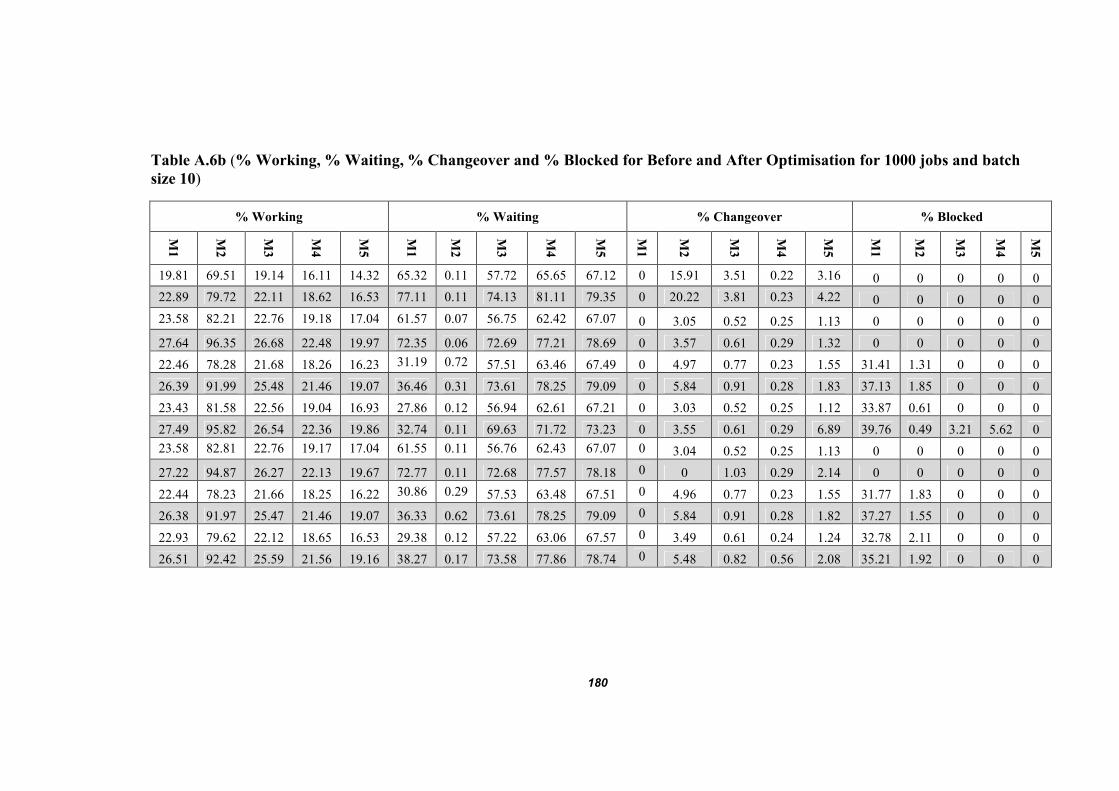
180


size 10)


M1

M2

M3

M4

M5

M1

M2

M3

M4

M5

M1

M2

M3

M4

M5

M1

M2

M3

M4

M5

19.81 69.51 19.14 16.11 14.32 65.32 0.11 57.72 65.65 67.12 0 15.91 3.51 0.22 3.16 0 0 0 0 0

22.89 79.72 22.11 18.62 16.53 77.11 0.11 74.13 81.11 79.35 0 20.22 3.81 0.23 4.22 0 0 0 0 0

23.58 82.21 22.76 19.18 17.04 61.57 0.07 56.75 62.42 67.07 0 3.05 0.52 0.25 1.13 0 0 0 0 0

27.64 96.35 26.68 22.48 19.97 72.35 0.06 72.69 77.21 78.69 0 3.57 0.61 0.29 1.32 0 0 0 0 0

22.46 78.28 21.68 18.26 16.23 31.19 0.72 57.51 63.46 67.49 0 4.97 0.77 0.23 1.55 31.41 1.31 0 0 0

26.39 91.99 25.48 21.46 19.07 36.46 0.31 73.61 78.25 79.09 0 5.84 0.91 0.28 1.83 37.13 1.85 0 0 0

23.43 81.58 22.56 19.04 16.93 27.86 0.12 56.94 62.61 67.21 0 3.03 0.52 0.25 1.12 33.87 0.61 0 0 0

27.49 95.82 26.54 22.36 19.86 32.74 0.11 69.63 71.72 73.23 0 3.55 0.61 0.29 6.89 39.76 0.49 3.21 5.62 0

23.58 82.81 22.76 19.17 17.04 61.55 0.11 56.76 62.43 67.07 0 3.04 0.52 0.25 1.13 0 0 0 0 0

27.22 94.87 26.27 22.13 19.67 72.77 0.11 72.68 77.57 78.18 0 0 1.03 0.29 2.14 0 0 0 0 0

22.44 78.23 21.66 18.25 16.22 30.86 0.29 57.53 63.48 67.51 0 4.96 0.77 0.23 1.55 31.77 1.83 0 0 0

26.38 91.97 25.47 21.46 19.07 36.33 0.62 73.61 78.25 79.09 0 5.84 0.91 0.28 1.82 37.27 1.55 0 0 0

22.93 79.62 22.12 18.65 16.53 29.38 0.12 57.22 63.06 67.57 0 3.49 0.61 0.24 1.24 32.78 2.11 0 0 0

26.51 92.42 25.59 21.56 19.16 38.27 0.17 73.58 77.86 78.74 0 5.48 0.82 0.56 2.08 35.21 1.92 0 0 0

181


Dominant S

olutio

n

Experim

ent T

ype

Mach

ine F

ailu

re


Queu

e for M

1

Queu

e for M

2

Queu

e for M

3

Queu

e for M

4

Queu

e for M

5

Queu

e for M

1

Queu

e for M

2

Queu

e for M

3

Queu

e for M

4

Queu

e for M

5

Before

Optimisation

yes 667.62 25691.39 1.67 0.01 0.54 12 791 0 0 0

No 975.13 33761.66 3.51 2.28 2.71 11 776 0 0 0

Lead Tim

e

Job Sequence

Optimisation

yes 1459.04 9256.12 53.02 2.42 2.44 50 581 3 0 0

No 938.01 6898.36 26.37 0.01 0.3 38 509 1 0 0

Buffer Size

Optimisation

yes 15.05 31.12 11.24 2.19 2.47 0 2 0 0 0

No 12.07 26.02 1.05 0.01 0.24 0 2 0 0 0

Job Sequence

and Buffer Size

Optimisation

yes 515.16 255.02 17.2 2.55 10.33 17 16 1 0 0

No 11.54 147.29 13.07 0.07 0.28 0 11 1 0 0

Total In

ven

tory

Holding Cost

Job Sequence

Optimisation

yes 1163 8408.11 57.28 2.53 2 40 528 3 0 0

No 938 6898.36 26.37 0.01 0.3 38 509 1 0 0

Buffer Size

Optimisation

yes 15.01 15.07 3.09 2.25 2 0 1 0 0 0

No 11.59 12.03 0.54 0 0.23 0 1 0 0 0

Job Sequence

and Buffer Size

Optimisation

yes 15.12 15.12 3.04 2.22 1.75 0 1 0 0 0

No 11.53 12.17 0.54 0 0.32 0 1 0 0 0

182


size 1)


M1

M2

M3

M4

M5

M1

M2

M3

M4

M5

M1

M2

M3

M4

M5

M1

M2

M3

M4

M5

7.4 31.2 7.6 6.7 6.4 77.8 0.1 68.9 75.3 58.8 0 59.5 2.9 0.1 20.5 0 0 0 0 0

9.5 40.2 9.8 8.6 8.3 90.5 0.3 87.3 91.3 71.1 0 53.9 3.4 0.1 19.7 0 0 0 0 0

20 83.56 20.41 18 17.27 65.59 0.02 59.1 64.09 67.25 0 1.52 0.26 0.12 0.56 0 0 0 0 0

23.25 98.17 24 21.03 20.29 77 0.03 76 79 79.03 0 1.79 0.31 0.14 1 0 0 0 0 0

19.08 80.51 20 17.26 17 32.11 0.45 59.3 65 68 0 2.55 0.39 0.12 1 34.11 1.51 0.43 0 0

22.47 95 23.18 20.33 20 37.25 0.13 76.35 79.52 79.45 0 3 0.46 0.14 1 40.27 2.03 0 0 0

19.47 82.23 20.09 18 17 32 0.07 59.38 64.25 66.05 0 1.7 0.31 0.2 2.04 34.24 1.11 0 0 0

23 97 24 21 20.03 36.39 0.27 76 79.08 79.3 0 1.76 0.3 0.14 1 41 1.04 0.08 0 0

20 83.56 20.41 18 17.27 65.59 0.03 59.1 64.09 67.25 0 1.52 0.26 0.12 0.56 0 0 0 0 0

23.25 98.17 24 21.03 20.29 77 0.03 76 79 79.03 0 1.79 0.31 0.14 1 0 0 0 0 0

19 79 19.23 17 16.27 32.39 0.34 60.08 65 68.09 0 2.45 0.38 0.11 1 34.25 4 0.03 0.28 0

22.46 95 23.17 20.32 20 37.17 0.11 76.36 79.53 79.46 0 3 0.45 0.14 1 40.36 2.08 0 0 0

19 79.07 19.32 17 16.34 32.02 0.31 60.2 65 68.22 0 1.73 0.24 0.16 0.53 35 4.01 0 0 0

22.5 95 23.21 20.35 20 37.12 0.07 76.36 79.44 79.4 0 2.82 0.41 0.19 1 40.37 2.09 0 0 0

183


Dominant S

olutio

n

Experim

ent T

ype

Mach

ine F

ailu

re


Queu

e for M

1

Queu

e for M

2

Queu

e for M

3

Queu

e for M

4

Queu

e for M

5

Queu

e for M

1

Queu

e for M

2

Queu

e for M

3

Queu

e for M

4

Queu

e for M

5

Before

Optimisation

yes 7224.87 13668.1 0.41 0.01 0.22 547 977 0 0 0

No 9259.76 16269.6 8.21 2.45 3.71 246 787 0 0 0

Lead Tim

e

Job Sequence

Optimisation

yes 3025.03 10572.4 35.69 2.54 1.85 104 664 2 0 0

No 2926.12 10340.2 36.49 0.01 0.24 119 763 2 0 0

Buffer Size

Optimisation

yes 51.75 132.85 5.19 2.23 1.91 2 8 0 0 0

No 42.96 71.44 1.05 0.01 0.24 2 5 0 0 0

Job Sequence

and Buffer Size

Optimisation

yes 182.01 82.41 7.49 2.43 0.86 6 5 0 0 0

No 154.42 139.07 6.49 0.06 0.22 6 10 0 0 0

Total In

ven

tory

Holding Cost

Job Sequence

Optimisation

yes 3025.03 10572.4 35.69 2.54 1.85 104 664 2 0 0

No 2926.12 10340.2 36.49 0.01 0.24 119 763 2 0 0

Buffer Size

Optimisation

yes 51.59 67.83 3.83 2.39 1.94 2 4 0 0 0

No 43.66 58.03 0.54 0.01 0.23 2 4 0 0 0

Job Sequence

and Buffer Size

Optimisation

yes 50.71 68.15 2.94 1.85 1.71 2 4 0 0 0

No 42.54 57.28 0.56 0.05 0.12 2 4 0 0 0

184


size 5)


M1

M2

M3

M4

M5

M1

M2

M3

M4

M5

M1

M2

M3

M4

M5

M1

M2

M3

M4

M5

15.22 63.91 15.73 13.82 13.32 69.93 0.71 60.67 65.62 66.51 0 20.54 3.42 2.74 5.25 0 0 0 0 0

35.84 59.26 21.23 24.81 9.54 64.12 0.12 70.71 75.13 90.45 0 40.74 8.13 0.13 0.13 0 0 0 0 0

19.78 83.54 20.41 17.91 17.27 65.57 0.05 59.11 64.11 67.26 0 1.52 0.26 0.12 0.56 0 0 0 0 0

23.25 98.17 23.99 21.03 20.29 76.74 0.03 75.69 78.81 79.03 0 1.79 0.31 0.14 0.66 0 0 0 0 0

19.25 81.28 19.86 17.41 16.8 32.02 0.12 59.68 64.58 67.63 0 1.78 0.25 0.12 0.65 33.85 1.91 0.02 0 0

22.47 94.87 23.18 20.33 19.61 37.75 0.12 76.34 79.52 79.45 0 0.96 0.46 0.14 0.92 39.77 2.04 0 0 0

19.53 81.88 20.12 17.64 17.04 31.11 0.06 58.96 64.32 67.51 0 1.46 0.26 0.12 0.55 34.66 1.72 0.46 0 0

22.84 96.45 23.57 20.66 19.94 36.53 0.03 76.11 79.01 79.41 0 1.75 0.31 0.14 0.65 40.62 1.74 0 0.18 0

19.78 83.54 20.41 17.91 17.27 65.57 0.05 59.11 64.11 67.26 0 1.52 0.26 0.12 0.56 0 0 0 0 0

23.25 98.17 23.99 21.03 20.29 76.74 0.03 75.69 78.81 79.03 0 1.79 0.31 0.14 0.66 0 0 0 0 0

19.13 80.77 19.73 17.31 16.71 32.27 0.16 59.76 64.71 67.73 0 2.08 0.31 0.12 0.65 33.93 2.09 0.1 0 0

22.46 94.84 23.17 20.32 19.61 37.67 0.11 76.36 79.53 79.46 0 2.95 0.45 0.14 0.92 39.86 2.09 0 0 0

18.89 78.75 19.46 17.06 16.47 33.41 0.08 58.38 64.85 67.95 0 2.01 0.35 0.19 0.67 33.02 4.29 1.62 0 0

22.59 95.39 23.3 20.44 19.72 37.76 0.07 76.21 79.13 79.36 0 2.34 0.41 0.19 0.91 39.64 2.18 0.06 0.22 0

185


Dominant S

olutio

n

Experim

ent T

ype

Mach

ine F

ailu

re


Queu

e for M

1

Queu

e for M

2

Queu

e for M

3

Queu

e for M

4

Queu

e for M

5

Queu

e for M

1

Queu

e for M

2

Queu

e for M

3

Queu

e for M

4

Queu

e for M

5

Before

Optimisation

yes 3547.87 17004.11 16.33 2.45 6.55 104 908 0 0 0

No 2984.67 14883.21 2.96 0.01 0.81 101 916 0 0 0

Lead Tim

e

Job Sequence

Optimisation

yes 3554.28 12407.83 53.09 2.58 2.38 122 779 2 0 0

No 2902.05 10030.81 35.98 2.73 9.74 117 741 2 0 1

Buffer Size

Optimisation

yes 97.07 135.66 7.05 2.32 1.96 3 8 0 0 0

No 81.75 128.59 2.46 0.01 0.24 3 9 0 0 0

Job Sequence

and Buffer Size

Optimisation

yes 173.59 211.55 17.18 1.76 1.76 6 13 1 0 0

No 80.41 328.07 11.42 0.01 0.31 3 24 1 0 0

Total In

ven

tory

Holding Cost

Job Sequence

Optimisation

yes 3961.39 10913.21 38.57 2.41 2.02 113 685 2 0 0

No 2733.87 9045.92 38.84 0.01 0.33 111 667 2 0 0

Buffer Size

Optimisation

yes 97.07 135.66 7.05 2.32 1.96 3 8 0 0 0

No 82.24 115.11 2.92 0.01 0.24 3 8 0 0 0

Job Sequence

and Buffer Size

Optimisation

yes 94.48 132.81 7.31 2.19 1.86 3 8 0 0 0

No 80.68 114.06 0.08 0.02 0.22 3 8 0 0 0

186


size 10)


M1

M2

M3

M4

M5

M1

M2

M3

M4

M5

M1

M2

M3

M4

M5

M1

M2

M3

M4

M5

16.81 71.12 17.14 15.22 14.72 68.41 0.11 60.12 66.14 65.53 0 14.14 2.21 0.51 4.93 0 0 0 0 0

19.43 81.91 20.11 18.34 16.91 80.62 0.11 77.71 80.62 78.22 0 18.12 2.22 1.01 4.84 0 0 0 0 0

19.79 83.56 20.41 17.91 17.27 65.59 0.02 59.11 64.09 67.25 0 1.52 0.26 0.12 0.56 0 0 0 0 0

23.25 98.17 23.99 21.03 20.29 76.74 0.03 75.69 78.81 79.03 0 1.79 0.31 0.14 0.66 0 0 0 0 0

19.02 80.61 19.69 17.27 16.66 32.88 0.22 59.73 64.71 67.66 0 2.51 0.39 0.12 0.78 33.33 1.76 0 0 0

22.47 94.87 23.18 20.33 19.61 38.37 0.21 76.35 79.52 79.45 0 2.96 0.46 0.14 0.92 39.15 1.95 0 0 0

19.58 82.92 20.19 17.67 17.08 30.77 0.06 59.17 64.31 67.46 0 1.51 0.26 0.12 0.55 34.95 1.28 0 0 0

22.91 96.76 23.64 20.73 20.01 37.61 0.06 76.04 79.11 79.33 0 1.76 0.31 0.14 0.65 33.46 1.41 0 0 0

19.78 83.54 20.41 17.91 17.27 65.57 0.05 59.11 64.11 67.26 0 1.52 0.26 0.12 0.56 113 685 2 0 0

23.24 98.15 23.98 21.03 20.29 76.75 0.05 75.71 78.82 79.04 0 1.78 0.31 0.41 0.66 111 667 2 0 0

19.09 80.61 19.69 17.27 16.66 32.88 0.22 59.73 64.71 67.66 0 2.51 0.39 0.12 0.78 3 8 0 0 0

22.46 94.86 23.18 20.32 19.61 38.31 0.25 76.35 79.52 79.45 0 2.96 0.46 0.14 0.92 3 8 0 0 0

19.33 81.19 19.89 17.46 16.85 33.23 0.06 59.45 64.51 67.56 0 2.11 0.33 0.12 0.69 3 8 0 0 0

22.52 95.11 23.24 20.38 19.66 39.11 0.06 76.18 79.31 79.41 0 2.75 0.56 0.14 0.92 3 8 0 0 0

187

Appendix B – Developed Graphical User Interface for Combinatorial Optimisation (SIM-Prove)

Figure B.1 (Setting the Simulation Parameters for Optimisation Process)

188

Figure B.2 (Genetic Algorithms Optimisation Parameters)

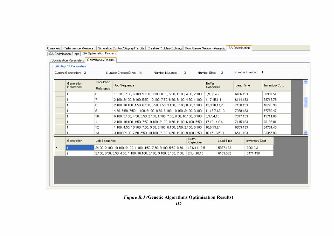
189

Figure B.3 (Genetic Algorithms Optimisation Results)

190

Appendix C – Optimisation Model Implementation

Step 1: Open Simulation Model and Set the Simulation Parameters

1. Set the warm-up period for simulation if required.

2. Set the run time for the simulation model.

3. Set the process batch size for the simulation model.

4. Set the work type for the simulation model.

5. Set the halt limit for simulation model.

6. Set the visible state of model i.e. either true or false.

Step 2: Set the Initial Parameters for the Optimisation Model

1. Set population size i.e. 20.

2. Set number of generations i.e. 100.

3. Set initial crossover rate i.e. 70% (Subjected to change as solution evolves).

4. Set number of inverted solutions i.e. 1.

5. Set number of elite solutions i.e. 2.

6. Set number of mutated solutions i.e. 3 (Derived from crossover rate).

7. Set the optimisation criteria i.e. either buffer size or job sequence or both.

8. Set the fitness function lead time and total inventory holding cost.

191

Step 3: Run Genetic Algorithms Optimisation Framework

1. Generate initial population of buffer size and job sequence.

2. Evaluate each individual from the population. Here evaluation is based on the

model developed in the Simul8.

3. Sort the results according to the fitness functions, where fitness functions are

transformed to single objective using random weights for sorting.

4. Use genetic operators to generate the next generation according to the set

parameters;

4.1 Elitism.

4.2 Crossover.

4.3 Mutation.

4.4 Inversion.

5. Save two Elite Solutions from each generation.

6. If stopping criteria is reached then,

6.1 Display results.

6.2 Copy and save results to file.

7. Else go to Step 1.

improving manufacturing systems using integrated discrete event simulation and evolutionary

Documents