improving link-state routing - by using … · improving link-state routing -by using estimated...

December 12, 2002

IMPROVING LINK-STATE ROUTING - BY USING ESTIMATED FUTURE LINK DELAYS

(REVISED)+∗×

Hyeonsang Eom

[email protected]

Institute for Advanced Computer Studies Computer Science Department

University of Maryland College Park, 20742

CS-TR-4297R

UMIACS-TR-2001-75R

December 12, 2002 ABSTRACT In link-state routing, routes are determined based on estimates of the current delays on the

links. Ideally, a data packet should be routed based on the delays it will encounter at each link

of the path at the time the packet gets to the link. To address this issue, we have developed a

new approach that improves link-state routing by estimating and using the future link delays

encountered by data packets. In link-state routing, link-delay estimates are periodically flooded

throughout the network. This flooding of link-delay estimates is done without considering the

relevance of these estimates to routing quality. Our approach also improves link-state routing

by broadcasting these estimates only to the extent that they are relevant. Simulation studies

+ This work is supported partly by DARPA/Rome Labs, Department of the Air Force, under contract F306020020578 to the Department of Computer Science at the University of Maryland. The views, opinions, and/or findings contained in this report are those of the author(s) and should not be interpreted as representing the official policies, either expressed or implied, of the Department of Air Force, DARPA, DOD, or the U.S. Government. ∗ This work was supported in part by the Maryland Information and Network Dynamics (MIND) Laboratory, its Founding Partner Fujitsu Laboratories of America, and by the Department of Defense through a University of Maryland Institute for Advanced Computer Studies (UMIACS) contract. × This report is a revised version of the report titled Information Dynamics applied to link-state routing.

1

Report Documentation Page Form ApprovedOMB No. 0704-0188

Public reporting burden for the collection of information is estimated to average 1 hour per response, including the time for reviewing instructions, searching existing data sources, gathering andmaintaining the data needed, and completing and reviewing the collection of information. Send comments regarding this burden estimate or any other aspect of this collection of information,including suggestions for reducing this burden, to Washington Headquarters Services, Directorate for Information Operations and Reports, 1215 Jefferson Davis Highway, Suite 1204, ArlingtonVA 22202-4302. Respondents should be aware that notwithstanding any other provision of law, no person shall be subject to a penalty for failing to comply with a collection of information if itdoes not display a currently valid OMB control number.

1. REPORT DATE 12 DEC 2002 2. REPORT TYPE

3. DATES COVERED 00-00-2002 to 00-00-2002

4. TITLE AND SUBTITLE Improving Link-State Routing -By Using Estimated Future Link Delays(Revised)

5a. CONTRACT NUMBER

5b. GRANT NUMBER

5c. PROGRAM ELEMENT NUMBER

6. AUTHOR(S) 5d. PROJECT NUMBER

5e. TASK NUMBER

5f. WORK UNIT NUMBER

7. PERFORMING ORGANIZATION NAME(S) AND ADDRESS(ES) University of Maryland,Institute for Advanced Computer Studies,College Park,MD,20742

8. PERFORMING ORGANIZATIONREPORT NUMBER

9. SPONSORING/MONITORING AGENCY NAME(S) AND ADDRESS(ES) 10. SPONSOR/MONITOR’S ACRONYM(S)

11. SPONSOR/MONITOR’S REPORT NUMBER(S)

12. DISTRIBUTION/AVAILABILITY STATEMENT Approved for public release; distribution unlimited

13. SUPPLEMENTARY NOTES The original document contains color images.

14. ABSTRACT

15. SUBJECT TERMS

16. SECURITY CLASSIFICATION OF: 17. LIMITATION OF ABSTRACT

18. NUMBEROF PAGES

34

19a. NAME OFRESPONSIBLE PERSON

a. REPORT unclassified

b. ABSTRACT unclassified

c. THIS PAGE unclassified

Standard Form 298 (Rev. 8-98) Prescribed by ANSI Std Z39-18

December 12, 2002

suggest that our approach can lead to significant reductions in routing traffic with noticeable

improvements of routing quality in high-load conditions.

1 Introduction

In a packet switched network a collection of nodes, consisting of computing machines, is

connected using communication links capable of transferring information in the form of

packets, from one node to another. When a direct link does not exist from the source node

and the destination node, but a path via one or more intermediate nodes exists, the packets

from the source node follow this path, such that each intermediate node carries out a store-

and-forward operation until the packets are delivered to the destination node. The path is

determined through “routing” techniques. Clearly routing is an operation which has to reply

on the global state of the network. Several techniques have been used for collecting and using

global information for routing. One such technique is link-state routing in which each node

collects information on the state of its outgoing links, usually in the form of the waiting time,

and shares it with all other nodes in the network. Based on the link-state information collected,

a node may determine the “best” path from it to any other node of the network.

In link-state routing, we refer to the global link-state information that each node maintains and

uses for routing, as a view. The view is essentially a graph with vertices corresponding to the

network nodes, edges corresponding to network links, and for each link, a cost representing an

estimate of the current delay on the link. Based on its view, each node determines least-cost

paths to all other nodes as the best paths. The end-to-end cost function is the sum of the costs

at all the links in the route.

Each node makes (periodic and/or event-driven) measurements of the current delay for each

of its outgoing links. It periodically constructs an estimate for the current delay on the link

from these measurements as link-cost estimates, and sends these link-delay estimates to all

other nodes in the network. When broadcasting, a node sends link-delay estimates for its

outgoing links to its neighbors, and each of the neighbors in turn sends these estimates to its

neighbors, and this continues until all nodes receive the estimates. This broadcast technique is

referred to as flooding [Peterson, 1996; Rosen, 1980]. When each node constructs a link-delay

estimate for a local link (i.e., a link going from it) or receives an estimate for a remote link, it

updates its view (view update). Each node periodically uses its current information about the

2

December 12, 2002

network to compute least-cost paths to all other nodes (periodic route update) by using the

standard shortest-path algorithm [Dijkstra, 1959]. These least-cost paths are used by the node

to route data packets, i.e. when the node receives a data packet, it forwards the packet to the

neighbor that is the next node in the least-cost path to the destination node of the packet.

Consider a node with a link l outgoing from it. Let x denote the delay on the link and

represent time. Assume that this node has made delay measurements, , , …, on

this link at time t , , …, , respectively, before the current time , where is the

total number of measurements and time precedes if i <

t

nx− )1( −− nx

0t

1−x

n− )1( −− nt 1−t n

it jt j . Say the node makes an

estimate of the current link delay using these previous delay measurements. Let

denote this delay estimate. In link-state routing, is

periodically computed and flooded to all other nodes so that each node can use this estimate as

the cost of link l when computing least-cost paths to all other nodes.

),...,,(ˆ )1(0 −−− xxx nn 1−x )1−x,...,, ( −−− x nn(ˆ0 xx )1

In link state routing, there is a key issue to consider: each node creates a delay estimate for

an outgoing link and sends it to all nodes. This estimate is based on measurements made in the

past and its value to a receiving node may decrease over time, to the point that the new

estimate may not lead to any changes in the view of a node receiving it. In this report, we

examine this issue by reflecting the changes in the estimates over time and take such changes

into account for not only the routing decisions but also the flooding decisions.

x̂

1.1 Link State

Many variations of the standard link-state-routing approach described above have been

proposed, where link-state information in forms other than that of link delays is used in

routing (this means that link costs do not represent delays). This is primarily because the ways

that link delays have been used can lead to inferior routing performance, say due to routing

instabilities. For example, routing performance can be degraded because of routing

oscillations, where given two links connecting two regions of a network, the preferred route

from one region to the other for most or all inter-region traffic is constantly switched because

most or all traffic shifts at the same time due to all nodes’ simultaneous adjustment of their

routes with the same reported delay values for the links [Khanna, 1989].

3

December 12, 2002

Historically, the original ARPANET used queue length as the link-cost metric. However, this

metric was not effective because it did not take either link bandwidth or the latency into

account. The original scheme was revised to consider the bandwidth and latency by using delay

averages as link costs. However, this revised scheme caused routing instabilities under heavy

load, resulting in routing oscillations. For stable routing, the ARPANET metric was again

revised to a hop-normalized-utilization function [Khanna, 1989]. This function computes a

link cost by normalizing an estimate of the link utilization via a linear transformation after

making this estimate with measured delay values. (The idea behind this computation is hop-

normalization, which means normalization of the utilization in terms of hops so that the

resulting cost is relative to that of alternative links. To illustrate how routing is done based on

this idea, consider the case where 61 is reported as the cost of a link and 20 is reported as

that of an alternative link l . In this case, with additional 2 hops is used in routing before l .)

This new approach smoothed the temporal variation of the metric by using link utilization

rather than link delay and using a movement (metric-change) limit, and compressed the

dynamic range of the metric by limiting the cost-value range and considering the link type.

However, the benefit of using this kind of technique to damp out sudden changes or routing

oscillations depends on the network and/or traffic pattern. Recently, there was an attempt to

tune the parameters in the link-cost function via online simulation [Kaur, 2000]. Also,

congestion-based metrics were proposed [Glazor, 1990]. However, these metrics have been

unpopular because the use of the metrics may lead to routing instabilities [Kaur, 2000].

1l

2 2l 1

In some cases, link costs are not recalculated dynamically and constant link costs are used most

of the times. In these cases, the computation and broadcast of link costs for route updates are

not periodic. For example, link costs are set statically by a network administrator, and these

costs are changed only in case of link failure. This static approach may be effective in some

small-scale networks in which there are few or no alternative paths. However, the approach

may not be suitable for most networks in which there are many alternate paths, because

different alternate paths may become more or less desirable as link delays change over time.

1.2 Approach

In link-state routing, each node makes link-delay estimates based solely on information

provided in the past, and uses these estimates in routing. Ideally, a data packet should be

4

December 12, 2002

routed based on the delays it will encounter at each link of the path at the time the packet gets

to the link. That is, for each link along a potential route, the node doing the routing needs an

estimate of the link delay at the (future) time when the data packet would arrive at the link. We

refer to this future delay as encountered delay. To address the issue that routing should be

done based on encountered delay, we have developed a new approach to consider

encountered delay in routing by estimating this delay via a projection technique. This technique

is described in Section 3. Before presenting our approach, Section 2 provides a formal

description of the problem of estimating encountered delay and using this delay to determine

least-cost paths in routing.

Also, in link-state routing, each node floods its link-cost estimates without regard to whether

the estimates are necessary for determining least-cost paths. This could result in a significant

amount of unnecessary routing traffic. In our approach, each node disseminates link-cost

information only when necessary for estimating encountered delay. We have found that our

approach leads to reductions in routing traffic as well as improvements in data performance

(e.g. delay, throughput). Section 3 also presents this selective-broadcast technique. Our

experiments and the results are presented in Section 4. In this section, we describe the network

configuration and scenarios for our simulation studies, and present the comparison results

obtained from these studies. Section 5 briefly surveys major related works. Finally, Section 6

concludes our work and summarizes our future work.

5

December 12, 2002

2 Problem Formulation

For a link, we treat the delay x at time t as a stationary stochastic process { . Thus, the

mean and variance of are constant (independent of time ). Let and denote the

mean and variance, respectively. Also, the autocorrelation function

)}(tx

2σ)(tx t m

2}])(}{)([{ τtxmtxE +− σm− depends only on the lag τ and not on time . Let t )(τρ

denote this autocorrelation function.

Consider the instantaneous conditional mean and variance, respectively, of the delay given a

measurement at time : 0x 0t

})(|)({ 00 xtxtxE = , where tt <0

})(|)({ 00 xtxtxVar = , where t t<0

If no other measurement is available, we expect the instantaneous conditional mean to change

from towards over time. Similarly, we expect that the instantaneous conditional

variance to change from zero to over time. When the measurement is made, the

conditional variance is zero because the true value of

0x m

2σ

x is observed at that time.

For the determination of least encountered-delay paths and the selective broadcast of link-

delay information, we require estimates for the functions and

. Based on the steady-state behavior explained above, we need

techniques for estimating these function values. The routing problem that we address is how

to use these estimates in route determination and selective broadcast.

})(|)({ 00 xtxtxE =

})(|)({ 00 xtxtxVar =

6

December 12, 2002

3 Approach

We assume that the conditional mean decays exponentially over time to its steady-state value.

Based on this assumption, we use

)1)((),,(ˆ )0(0000

ttexmxttxm −−−−+= α ( ) 0tt ≥

as an estimate of , where })(|)({ 00 xtxtxE = α is a non-negative constant. This is illustrated

in Figure 1. Similarly, we use an exponential-decaying estimate for

, as illustrated in Figure 2.

),,(ˆ 002 ttxσ

}0x=)(|)({ 0txtxVar

0t t

m

0x

),,(ˆ 00 ttxm

Figure 1 Evolution of the instantaneous conditional delay-mean estimate

0t

2σ

t0

),,(ˆ 002 ttxο

Figure 2 Evolution of the instantaneous conditional delay-variance estimate

7

December 12, 2002

Theorem If is a stochastic process and has the following additive form for a

constant and a positive constant

)(tx

m t∆ :

)()1(})({)( tmtxmttx υββ −+−=−∆+ ,

then

(i) , Var is a constant (denoted by ), and the autocorrelation function mtxE =)}({ )}({ tx 2σ

200 }])(}{)([{),( σρ mtxmtxEtt −−=

( t for a non-negative integer ) decreases exponentially as )(0 tkt ∆+= k 0tt − (or ) increases

(depending only on the lag), and

k

(ii) )},(1){(})(|)({ 00000 ttxmxxtxtxE ρ−−+== ,

where β is a constant such that 10 << β , and )(tυ is an independent white-noise process

such that 0)}({ =tE υ and Var (positive constant) (proof in

Appendix A on pages 23 to 26).

22{ υσυE )}( =t)}({υ =t

Note that this theorem is valid for arbitrary and t if there is a non-negative integer

such that

0t 0t≥ k

)(0 tktt ∆+= , where satisfies the additive model form. We can choose such

and . Thus, we can apply the theorem with respective to arbitrary t and .

t∆ k

t∆ 0 0tt ≥

Part (i) of the theorem implies that if has the additive form, then is stationary and its

autocorrelation function decreases exponentially in time. When we examined a sample

autocorrelation function for a set of Internet round-trip delay measurements made using the

NetDyn tool [Sanghi, 1993], we found that the function decays exponentially in the short term.

The additive form is a form that we work with. Based on Part (ii) of the theorem, we make the

assumption stated at the beginning of this section, that the conditional mean decays

exponentially over time. Refer to Appendix B (pages 27 and 28) for the additional theorem

that explains our motivation of using the exponential-decaying conditional delay-variance

estimate.

)(tx )(tx

8

December 12, 2002

Figure 3 shows a sample of Internet round-trip delay measurements, and Figure 4 shows a

sample autocorrelation function computed for this sample. The least-square estimates of α

for different sets of Internet round-trip delay measurements range from 58 sec to 73 sec .

Table 1 shows these values.

1− 1−

Figure 3 Round-trip times measured at 10 ms intervals between the University of Maryland at College Park and the University of Illinois at Chicago for 10 seconds

from 20:46 on 04/09/99

Figure 4 Sample autocorrelation function

Table 1 α values estimated with round-trip delay measurements made at 10 ms intervals between Maryland and Illinois for different start-times and durations

on 04/09/99 (via sample autocorrelation functions)

Duration (Seconds) Start-Time 10 20 30

20:46 67 71 58 20:51 73 66 69

9

December 12, 2002

Given these exponential-decaying estimation functions, a node computes the encountered

delay of a packet on a path as follows. Let the path have links , and let the node

send the packet into the path at time t . Let be the function estimating the

encountered delay on link at time t . The estimated encountered delay for the packet on link

is . The estimated encountered delay for the packet on link l is ,

and so on. So the estimated encountered delay for the packet on the path is given by:

...,,, 21 ll

2

nl

0 )(ˆ tm il

il

1l )(ˆ 01 tml ))(ˆ(ˆ 0

10

2 tmtm ll +

(...)ˆ...)))(ˆ(ˆ)(ˆ(ˆ))(ˆ(ˆ)(ˆ 01

02

01

03

01

02

01 nllllllll mtmtmtmtmtmtmtm ++++++++

Computing path costs in this way, the node would route the packet on the path with the least

encountered-delay estimate. Each node determines the least-cost paths using the standard

shortest-path algorithm as in link-state routing. Thus, routing is carried out as in standard link-

state routing except for the path-cost computation. To do this computation, each node

maintains a view as in link-state routing except that a measured delay and measurement time

are kept for each link. The node updates its view of a local link whenever a data packet is sent

on that link. The node updates its view of a remote link whenever it receives a measurement

update for the link. View updates are not periodic. Note that in our approach, link costs are

not considered as part of the link views in contrast to link-state routing.

At each view update for a link, each node updates the measured delay and measurement time

that it maintains for the link. Each node broadcasts the updated delay information to its

neighbors only if the estimated encountered delay on the corresponding link at that time is

significantly different from the steady-state mean. We assume that every node knows the

steady-state value of delay on each link. In our approach, the estimated encountered delay

becomes close to the corresponding steady-state value over time. Hence, no propagation of

updated delay information is required beyond some point. If a node does not receive any

measurement update for a link, it uses the steady-state value.

Each node maintains a routing table that indicates the next hop for each destination as in link-

state routing. In link-state routing, with its view for all links, each node periodically updates its

routing table by computing the least-cost paths to all the other nodes. However, in our

approach, each node computes link costs and updates routes just before it decides which of its

outgoing links to send the packet onto when it receives a data packet. We refer to this update

10

December 12, 2002

technique as the “just-in-time route-update” method. This method allows each node to

determine the current least-cost paths using the encountered delay estimated with the most

recent delay information for each link. Note that the periodic-update scheme used in link-state

routing is not suitable for our approach. The reason is that if the periodic-update scheme were

used, routes determined using our approach at each route-update time would be used without

any change until the next route-update time. The problem with this is that temporally-changing

estimated encountered delays cannot be used for routing of individual data packets. If link-

delay estimates made in the case of using the periodic scheme are close to the steady-state

values, the result of using the periodic scheme in our routing approach could be comparable to

that of using link-state routing. However, these link-delay estimates can be different from the

steady-state values. For example, consider the case where periodic route updates occur right

after link delays that are different from the steady-state values are measured. If these measured

values are used to make link-delay estimates at these route updates, these estimates are close or

equal to the measured values that are different from the steady-state values. Thus, the result of

using the periodic scheme can be negative.

We refer to our routing approach based on estimates of encountered delays as InfoDyn

routing. Table 2 summarizes the commonalities and differences between InfoDyn and the

standard link state routing approaches. In both approaches, each node measures the delay of a

data packet on each local link by time-stamping its arrival at the node and its departure from

the link queue, and adding this time difference to the sum of the packet transmission time (the

packet size divided by the link bandwidth) and link-propagation delay. We refer to a particular

node as a measurement node, and a node that uses the delay measurements made by this

measurement node for routing as a routing node. In this table, we focus on the measurement

node, local link, and routing node.

11

December 12, 2002

Table 2 Comparison of InfoDyn routing with standard link-state routing

Aspect InfoDyn Routing Standard Link-State Routing What Measurement and

Measurement Time Exponential Delay Average (Link Cost)

Who Measurement Node Measurement Node

How Measurement Exponential Averaging after Measurement

Link-View Construction

When Measurement Time (for View Update; When Each Data Packet Is Sent Out)

Periodically (for View Update)

How Conditional Broadcast Unconditional Flooding Link-View Transmission When Measurement Time

(for View Update) Periodically (for View Update)

Who Routing Node Routing Node View Update When When Each View Update Is

Received When Each View Update Is Received

What Encountered-Delay Estimate

Exponential Delay Average

Who Routing Node Measurement Node

How Exponential Model (with View)

Exponential Averaging (with Measurement)

Link-Cost Computation

When Route Update Periodically (for View Update and Subsequent Route Update)

What Least Encountered-Delay-Estimate Paths

Least Current-Delay-Estimate Paths

Who Routing Node Routing Node

How Standard Shortest-Path Algorithm

Standard Shortest-Path Algorithm

Route Update (Using Link Costs)

When Arrival of a Data Packet Periodically (Just after View Update)

12

December 12, 2002

4 Simulation

To show the overall applicability of this approach to link-state routing, we compared via

simulation a routing scheme using our approach with SPF (Shortest Path First), link-state

routing technique. For simulation studies, we used MaRS, the Maryland Routing Simulator

[Alaettinoglu, 1994; Shankar, 1992]. We tried SPF with two kinds of link-cost functions, a delay

cost function and a hop-normalized-utilization function [Khanna, 1989].

4.1 Network configuration and scenarios

We conducted studies for the NSFNET-T1-backbone topology. In this configuration, there

are 14 nodes connected via 21 links. Each link represents two one-way channels. Each node

can process a data packet of 544 bytes in 1 ms, and each link channel has 183 KB/s (1.4

Mbps) bandwidth. We assume that there is no propagation delay for each link because we

found that simulation results are not sensitive to the setting of propagation delay.

In this network, a workload is generated by FTP source and sink pairs. These sources and

sinks are connected to nodes. FTP is regulated by a flow-control mechanism and an

acknowledgement mechanism with retransmission. The flow-control mechanism is a static

window-based scheme implemented in MaRS. This scheme consists of two windows: produce

and send windows. We set the produce-window size to infinity, and the send-window size to

eight. Also, we use 120 seconds as the total simulated time.

There are two kinds of FTP flows: regular and on-off flows. In each regular flow, the source

starts transmitting packets at time 0, and sends as many packets as possible with an inter-

packet production delay of 1 ms. For each on-off flow, there are alternating constant-length on

and off intervals. Each on-off flow starts at a different time (from 0 to 24 seconds), and has a

different length (from 20 to 120 seconds). Also, a certain number of packets are produced at

once at the beginning of on intervals while no packets are produced during off intervals. The

number of packets for each on interval is determined so that the packets of that number would

be successively transmitted during the on interval without any flow-control mechanism and

without any other flow. Specifically, the number is the length of an on interval divided by the

transmission time of a data packet, where the transmission time is the packet size divided by

the link bandwidth.

13

December 12, 2002

We initially consider five scenarios in this network configuration: N0 – N4. The level of

queuing delay of these scenarios is high: in the best cases (lowest-average-delay cases after

cost-function-parameter tuning) of using SPF with 1 second route-update intervals, the

average queuing-delay portions of the average round-trip delay per packet are around 94 %.

Also, the utilizations (the average fractions of the time when packet queue size > 1) are around

0.73. There are 121 FTP flows in Scenario N0 to N3, and 131 flows in Scenario N4. Table 3

shows the differences between the scenarios. In particular, Scenario N4 has two hot spots

(each of which receives packets from every other node).

Table 3 Differences in the FTP-flow characteristics between scenarios

Scenario Number of Regular Flows

Number of On-Off Flows

Length of On-Off Intervals (Seconds)

N0 60 61 5 N1 60 61 10 N2 60 61 15 N3 0 121 5 N4 55 76 5

4.2 Results

For the InfoDyn scheme, we used an exponential-change-rate (α ) value and a threshold value

for the selective broadcast of routing packets, during each simulation run for each scenario.

We tried seven threshold values. Also, we tried eight α values across the full value range in

each of these different-threshold-value cases. As the steady-state value of each link in each

simulation run using the InfoDyn scheme, we used the sample delay mean of the

corresponding link computed in a simulation run using SPF with 1 second route-update

intervals for the same scenario.

The use of the InfoDyn scheme without any routing-packet broadcast (thereby with only local-

link view update) is called the InfoDyn Short-Term Steady-State (STSS) case. Hereafter, “best”

means leading to the lowest average round-trip delay per packet.

4.2.1 InfoDyn Short-Term Steady-State (STSS) case

In each scenario, we compared the InfoDyn STSS case of using the best α of the exponential

model with the best cases of using SPF with 1, 10, and 30 second route-update intervals - we

obtained the best result of using SPF for each combination of a route-update-interval length

14

December 12, 2002

and a scenario by tuning several cost-function parameters. In this comparison, the InfoDyn

case results in a 3 to 8 % reduction in the Average (Avg) Round-Trip (RT) delay per packet

and a 4 to 22 % reduction in the standard deviation (STD) in all scenarios. Figure 5 shows

these reductions. Note that there are no routing packets sent out in this InfoDyn case while

75,642, 7,602, and 2,562 routing packets are sent out with 1, 10, and 30 second route-update

intervals, respectively, in the SPF cases. These results imply that when every node knows the

“long-term” steady-state delay-mean values of all links and uses our routing approach, flooding

requirements can be significantly reduced (as in the InfoDyn STSS case) with noticeable

reductions in the average delay and the variance, compared with the standard link-state routing

approach where each node periodically broadcasts “short-term” steady-state values

(exponential averages) for link delays.

Reductions in the Avg RT Delay of InfoDyn STSS wrt SPF w/ Different

Route-Update Intervals

0

5

10

N0 N1 N2 N3 N4

Scenario

Perc

ent

Red

uctio

n in

th

e A

vg R

T D

elay

1 sec interval 30 sec interval

Reductions in the Avg-RT-Delay STD of InfoDyn STSS wrt SPF w/ Different

Route-Update Intervals

0

1020

30

N0 N1 N2 N3 N4

Scenario

Perc

ent

Red

uctio

n in

th

e A

vg-R

T-D

elay

STD



Figure 5 Reductions in the average round-trip delay and STD of InfoDyn STSS

4.2.2 Impact of routing-packet broadcast

For each scenario with a fixed α value, the average delay and STD are almost the same across

simulation runs with different threshold values, except for those runs in which a very large

number of routing packets are broadcast. For example, Figure 6 shows the impact of varying

the threshold value in Scenario N3 (the all-on-off case) when the best α is used. There are

three charts. The left-most and middle charts indicate the changes in the average delay and

STD, respectively, depending on the threshold value used. The right-most chart shows the

numbers of routing packets used for different threshold values. The smaller the threshold

value, the more routing packets are sent out. When about 40,000 routing packets are used (the

100 ms threshold-value case), there are 0.53 ms and 0.66 ms increases in the average delay and

15

December 12, 2002

STD, respectively, compared with 152.03 ms average delay and 92.24 ms STD of the best case

(the 130 ms threshold-value case). Similar impacts of routing-packet broadcast are observed

for the other scenarios. Appendix C (Figure A1 on pages 29 and 30) shows the same three

charts in each row for each of the other scenarios. As in Figure 6 (and also in Figure A1), for

the threshold values that correspond to less than 100,000 routing packets in each scenario, the

variation of the average delays is within 1 ms and that of STDs is within 5 ms. Note that these

numbers are the scale units of the delay and STD charts, respectively.

Avg RT Delay for Different Threshold Values

150

151

152

153

154

155

156

157

STSS 13

0

120

110

100 90 80

Threshold (ms)

Del

ay (m

s)

Avg RT Delay (ms)

Avg-RT-Delay STD for Different Threshold Values

85

90

95

100

105ST

SS 130

120

110

100 90 80

Threshold (ms)

Del

ay S

TD (m

s)

Avg-RT-Delay STD (ms)

The Number of Routing Packets for Different Threshold Values

0

100,000

200,000

300,000

400,000

500,000

STSS12

010

0 80

Threshold (ms)

Num

ber o

f Rou

ting

Pack

ets

Number of Routing Packets

Figure 6 Impact of varying the threshold in Scenario N3 (when using the InfoDyn scheme w/ the best α )

The average delay and STD range from 152.0 to 161.9 ms and from 89.7 to 109.1 ms,

respectively, in the best cases of using the InfoDyn scheme (with the best α ) in all scenarios

when routing packets are broadcast. Compared with this best case for each scenario, the

InfoDyn STSS case with the same best α leads to increases in the average delay and STD by

up to 0.1 ms and 0.3 ms, respectively. The reason why these increases are small is that the

impact of a routing packet on routing quality is transient: the encountered link delay estimated

by the receiving node using the delay measurement contained in the packet soon becomes

close to the steady-state value. These results indicate that each node may not need to broadcast

link-delay measurements when using the InfoDyn scheme.

16

December 12, 2002

4.2.3 Impact of varying the α value

There are two possible sources for the routing-quality improvement: use of the long-term

steady-state link-delay means and link-delay estimation with the exponential delay-mean

change. To see the influence of each of these factors, we first set α to infinity. Then, the link-

delay means are used without any change in route determination. In the InfoDyn STSS case,

this Static-Routing case leads to up to 5 % and 18 % increases in the average delay and STD,

respectively, in four scenarios and 2 % and 9 % decreases, respectively, in one scenario

compared with the best cases of using SPF. These results mean that the use of the link-delay

means is not a source of routing-quality improvement in most cases. However, the use of the

best α results in 4 to 11 % and 7 to 22 % decreases in the average delay and STD,

respectively, in all scenarios compared with these Static-Routing cases. These results indicate

that the selection of the α value is crucial for routing-quality improvement.

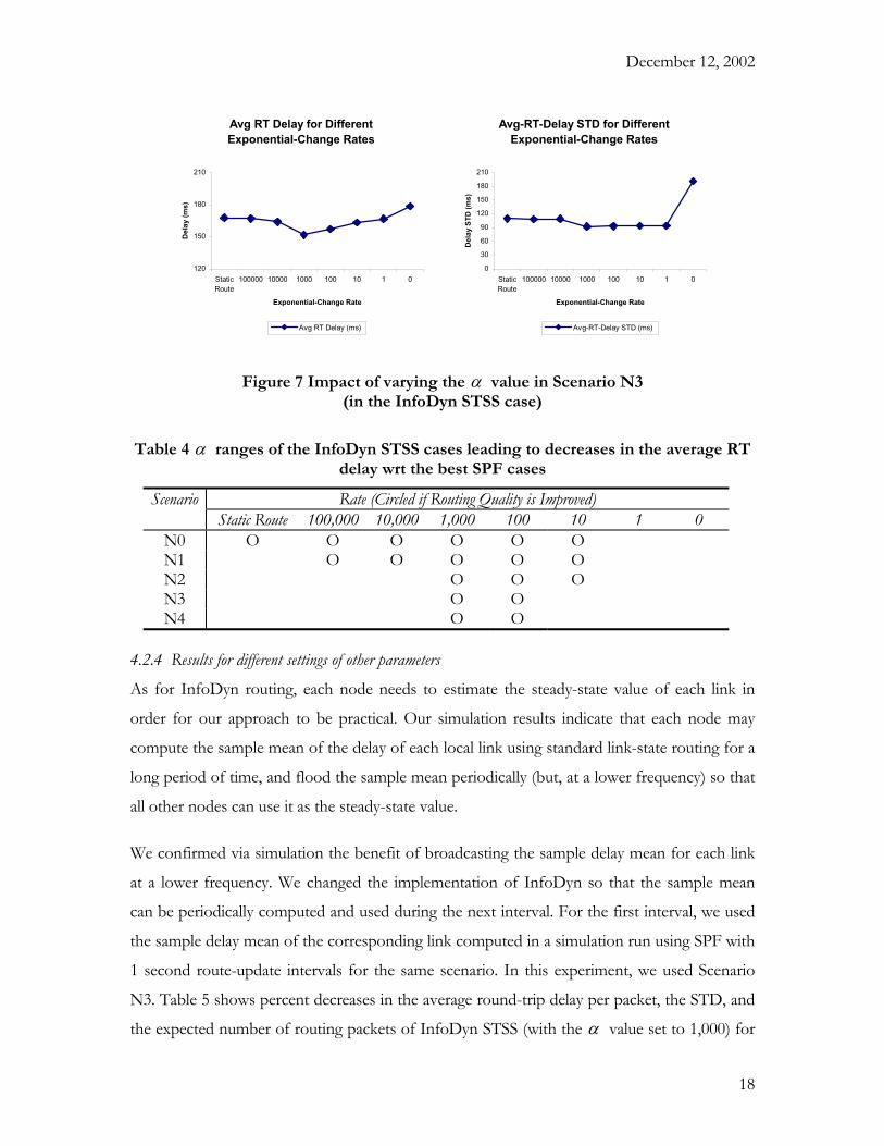
The best routing quality is achieved with the same α across all scenarios in the case of using

the same threshold value or in the InfoDyn STSS case. For example, Figure 7 shows the

effects of using different α values in Scenario N3 in the InfoDyn STSS case. The left and

right charts indicate the changes in the average delay and STD, respectively, depending on the

α value. As in the figure, the average delay and STD increase as the α value used digresses in

both directions from the value (1,000) for the best result. Similar trends are observed for the

other scenarios. Appendix D (Figure A2 on pages 31 and 32) shows the same two charts in

each row for each of the other scenarios. Therefore, if we can find the best or a near-best

setting in one case, we may reduce the average delay and STD by using the same setting in

other cases. In fact, routing quality is improved for a wide range of α values. Table 4 shows

the α ranges of the InfoDyn STSS cases in all scenarios that lead to decreases in the average

delay with respect to the best SPF cases. Therefore, the parameter tuning is not required.

17

December 12, 2002

Avg RT Delay for Different Exponential-Change Rates

120

150

180

210

StaticRoute

100000 10000 1000 100 10 1 0

Exponential-Change Rate

Del

ay (m

s)

Avg RT Delay (ms)

Avg-RT-Delay STD for Different Exponential-Change Rates

0

30

60

90

120

150

180

210

StaticRoute

100000 10000 1000 100 10 1 0


Del

ay S

TD (m

s)


Figure 7 Impact of varying the α value in Scenario N3 (in the InfoDyn STSS case)

Table 4 α ranges of the InfoDyn STSS cases leading to decreases in the average RT

delay wrt the best SPF cases

Rate (Circled if Routing Quality is Improved) Scenario Static Route 100,000 10,000 1,000 100 10 1 0

N0 O O O O O O N1 O O O O O N2 O O O N3 O O N4 O O

4.2.4 Results for different settings of other parameters

As for InfoDyn routing, each node needs to estimate the steady-state value of each link in

order for our approach to be practical. Our simulation results indicate that each node may

compute the sample mean of the delay of each local link using standard link-state routing for a

long period of time, and flood the sample mean periodically (but, at a lower frequency) so that

all other nodes can use it as the steady-state value.

We confirmed via simulation the benefit of broadcasting the sample delay mean for each link

at a lower frequency. We changed the implementation of InfoDyn so that the sample mean

can be periodically computed and used during the next interval. For the first interval, we used

the sample delay mean of the corresponding link computed in a simulation run using SPF with

1 second route-update intervals for the same scenario. In this experiment, we used Scenario

N3. Table 5 shows percent decreases in the average round-trip delay per packet, the STD, and

the expected number of routing packets of InfoDyn STSS (with the α value set to 1,000) for

18

December 12, 2002

different lengths of sample-mean update interval compared with the best SPF case with 1, 10,

and 30 second route-update intervals. Since 1 second interval length leads to the best result in

the case of using SPF, the percent change in the routing-packet number is estimated with

respect to that for 1 second interval length. As the table shows, if the sample mean is

broadcast at 40 second intervals, InfoDyn STSS is better than the best SPF in terms of the

average delay, the STD, and the expected number of routing packets used. However, as the

frequency increases, the benefit decreases or disappears.

Table 5 Percent decrease in the average delay, the STD, and the expected routing-packet number of InfoDyn STSS compared with the best SPF (w/ 1 second route-

update interval length) – negative numbers indicate percent increase

Decrease (%) Sample-Mean Broadcast Interval Length (sec.) of InfoDyn STSS

Average Delay per Packet

STD Expected Number of Routing Packets

40 3 2 98 30 1 -6 97 20 -5 -11 95 10 -9 -25 90

Currently high-speed networks are used in many places. We changed the experimental

environment to see whether or not the InfoDyn routing is effective in this situation. We used a

high-speed-network setting of 12.5 MB/s (100 Mbps) link-channel bandwidth, 0.4 ms data-

packet processing time, 5,000 byte data-packet size, and 200 send-window size in Scenario N3

(the all-on-off case). With this setting, the InfoDyn STSS with the best α (which is also 1,000)

of the exponential model results in a 2 to 5 % reduction in the average round-trip delay per

packet and a 3 % increase to 10 % decrease in the STD compared with the best cases of using

SPF with 1, 10, and 30 second route-update intervals. This result demonstrates that the

InfoDyn routing can also be effective for high-speed networks.

19

December 12, 2002

5 Related Work

Typically, delays vary and change rapidly in a network. For example, at a fine-grained level, the

characteristics of the Internet are highly dynamic [Agrawala, 1998]. Such dynamics in networks

make it difficult to estimate encountered link delays. Many researchers have investigated the

dynamic behavior of networks such as the dynamics of end-to-end Internet packet delays.

[Agrawala, 1998; Labowitz, 1998; Paxson, 1999; Pointek, 1997; Sanghi, 1993].

For statistical uncertainty modeling concerning information estimation, there are two basic

approaches: modeling based on past observations followed by extrapolation, and modeling via

the analysis of factors that determine the information at the target estimation time. An

example of the first modeling approach is a time-series model such as an AutoRegressive

Integrated Moving Average (ARIMA) model [Box, 1994; Chatfield, 1984]. An example of the

second is a regression model for factor(s)-and-effect information pairs (or tuples). The

parameters of both modeling approaches can be estimated using least-squares fitting [Trivedi,

1982].

Our research is fundamentally related to understanding the temporal dynamics of information

and information systems. Information plays a major role in the operation of systems. In

general, such information used in or generated by systems is also dynamic in nature. The

Information-Dynamics framework [Agrawala, 2000] provides a new perspective for systems

with a focus on information, information usefulness (or “value”), and the changes of

information and its usefulness over time. Hence, the framework allows us to better understand

the interactions between different components of a system. Such better understanding

provides a basis for better system design and implementation. We have performed research on

improving link-state routing from an information-dynamics perspective.

Many researchers have addressed time-related issues regarding the model of time and its

granularity, time representation, information processing, and distributed computing. Levi and

Agrawala [Levi, 1990] recognized the importance of an appropriate representation of time in a

variety of applications. Dyreson et al. [Dyreson, 2000] provided a formal model of time and its

granularity in a database context. Lamport [Lamport, 1978] defined the “happen before”

relationship as a partial ordering of events in distributed systems where entities communicate

20

December 12, 2002

via messages. Based on this relationship, Chandy [Chandy, 1985] developed an algorithm by

which an entity can compute a global state of the system.

Regarding information systems, many people have recently performed research on the

behavior of entities that exchange information. Kephart et al. [Kephart, 1998] investigated the

dynamics of an information-filtering economy. Later, Brooks et al. [Brooks, 2000] showed that

a price war in the information goods market can be avoided by taking on different strategies to

target a niche. There have also been attempts to model and/or predict e-commerce entities’

behavior using a stochastic model [Fader, 2000].

21

December 12, 2002

6 Conclusion and Future Work

Regarding link-state routing, we have studied the issue of estimating and using future link

delays. Our simulation results indicate that our approach to solve this problem is promising.

To address the future-delay issue, we developed a routing approach based on a new

exponential-model-based link-delay-estimation technique, and implemented a routing scheme

that uses this approach. When we compared this routing scheme with SPF via simulation for

various FTP-workload scenarios with the NSF-T1-backbone network topology, we found that

our routing scheme could achieve 100 % reductions in routing traffic with up to 8 % and 22 %

decreases of the average round-trip delay per packet and the standard deviation, respectively, in

high-load conditions. In comparison studies for the same experimental environment with a

high-speed-network setting, we found that our scheme could lead to 100 % reductions in

routing traffic with up to 5 % and 10 % decreases of the delay and the standard deviation,

respectively, in high-load conditions. These routing-traffic reduction and routing-quality

improvements resulted from the estimation of future (encountered) link delays based on the

dynamics of the expected link delay given an instantaneous link-delay measurement, and from

the consideration of the dynamic usefulness of the link-delay measurement via this estimation.

There will be various issues regarding the practical use of our approach. We plan to provide a

guideline for this practical use. In this direction, we will characterize the situations where we

can improve link-state routing by using our approach. This characterization study is important

for the practical use of our approach because simulation studies suggest that the benefit of

using this approach can vary depending on the pattern of the network workload and/or on the

characteristics of the network. For this research, we plan to investigate the effectiveness of our

approach via extensive simulation studies with different patterns of dynamic workload and/or

with different parameter settings for the network. Based on the results of these studies, we will

determine the characteristics of the situations that lead to significant routing-traffic reductions

with routing-quality enhancements in the case of using our approach, compared with standard

link-state routing.

22

December 12, 2002

Appendix

A. Theorem Proof

Theorem If is a stochastic process and has the following additive form for a

constant and a positive constant

)(tx

m t∆ :

)()1(})({)( tmtxmttx υββ −+−=−∆+ ,

then

(i) , Var is a constant (denoted by ), and the autocorrelation function mtxE =)}({ )}({ tx 2σ

200 }])(}{)([{),( σρ mtxmtxEtt −−=

( t for a non-negative integer ) decreases exponentially as )(0 tkt ∆+= k 0tt − (or ) increases

(depending only on the lag), and

k

(ii) )},(1){(})(|)({ 00000 ttxmxxtxtxE ρ−−+== ,

where β is a constant such that 10 << β , and )(tυ is an independent white-noise process

such that 0)}({ =tE υ and Var (positive constant) . 2υσ=

2 )}({υ t{)}( υ= Et

Proof:

Let us first prove Part (i).

The additive form can be rewritten as

)1()()1(})({)( LLLLLLLttmttxmtx ∆−−+−∆−=− υββ

By successive substitution in (1),

)2()()1())(2()1(

))](3()1(}))(3({[)()1())](2()1(}))(2({[)(

2

LLLLLLLLLLLLLLLLLLLLLLLLLLLM=∆−−+∆−−+

∆−−+−∆−=

∆−−+∆−−+−∆−=−

ttttttmttx

ttttmttxmtx

υββυβυβββ

υβυβββ

23

December 12, 2002

By using the eventual result of (2),

)3())}(({)1(

}))(3())(2()(){1()(

1

1

2

LLLLLLLLLLLLL

L

∑∞

=

− ∆−−=

+∆−+∆−+∆−−=−

i

i tit

ttttttmtx

υββ

υββυυβ

Taking the expectation on both sides of (3) yields

)4())}](({[)1(})({1

1 LLLLLLL∑∞

=

− ∆−−=−i

i titEmtxE υββ

Since 0)}({ =tE υ , it follows from (4) that

)5(0})({ LLLLLLLLLLLLL=−mtxE

Since , it follows from (5) that mtxEmtxE −=− )}({})({

)6()}({ LLLLLLLLLLLLLLmtxE =

Taking the expectation on the squares of both sides of (3) yields

)7())}](())(({[)1(

))}](({[)1(

]]))}(({[[)1(]})([{

1 ,1

112

1

2)1(22

2

1

122

L∑ ∑

∑

∑

∞

=

∞

≠=

−−

∞

=

−

∞

=

−

∆−∆−−+

∆−−=

∆−−=−

i ijj

ji

i

i

i

i

tjttitE

titE

titEmtxE

υυβββ

υββ

υββ

Since 0)}()({ 21 =ttE υυ if t , and , it follows from (7) that 21 t≠ 22 )}({ υσυ =tE

)8()1(]})([{1

)1(2222 LLLLLLLLLL∑∞

=

−−=−i

imtxE βσβ υ

Since 10 << β , it follows from (8) that

)9()}1()1({

)}1(1{)1(]})([{222

2222

LLLLLLLLLυ

υ

σββ

βσβ

−−=

−−=−mtxE

Since Var ]})([{)}({ 2mtxEtx −=

)10()}1()1({)}({ 222 LLLLLLLLLLυσββ −−=txVar

24

December 12, 2002

Since , and (3), )}({2 txVar=σ ∑∞

=

− ∆−−=−1

1 ))}(({)1()(i

i titmtx υββ

)11())}]()(())(({[)1(

]))}()(({))}(({[)1()),((

2

1 100

112

2

10

1

10

1200

συυβββ

συβυββρ

∑∑

∑∑∞

=

∞

=

−−

∞

=

−∞

=

−

∆−∆+∆−−=

∆−∆+∆−−=∆+

i j

ji

j

j

i

i

tjtkttitE

tjtkttitEttkt

Since 0)}()({ 21 =ttE υυ if t , , and 21 t≠ 22 )}({ υσυ =tE 10 << β , it follows from (11) that

)12(})1{()1(

)1(

}{)1()),((

2222

2

1

)1(222

2

1

211200

LLLLLLLσββσβ

σββσβ

σσβββρ

υ

υ

υ

−−=

−=

−=∆+

∑

∑∞

=

−

∞

=

−−+

ki

ik

i

ikittkt

Since 2222 )}1()1({ υσββσ −−= (10), it follows from (12) that

)13(

)),(( 2200

LLLLLLLLLLLLLk

kttktβ

σβσρ

=

=∆+

Therefore, mtxE =)}({ (6), Var is a constant (10), and since t and )}({ tx )(0 tkt ∆+=

10 << β , it follows from (13) that the autocorrelation function ),( 0ttρ decreases

exponentially as t (or ) increases (depending only on the lag). 0t− k

From now, let us prove Part (ii).

For t , it follows from the additive form that t∆+0

)14()()1(})({)( 000 LLLLLLLtmtxmttx υββ −+−=−∆+

For t , it follows from the additive form that tttt ∆+∆+=∆+ )()(2 00

)15()()1(})({))(2( 000 LLLLttmttxmttx ∆+−+−∆+=−∆+ υββ

It follows from (14) and (15) that

)16()}()(){1(})({

)()1()]()1(})({[))(2(

0002

0000

LLLtttmtxtttmtxmttx

∆++−+−=

∆+−+−+−=−∆+

υβυββ

υβυβββ

For t , it follows from the additive form that tttt ∆+∆+=∆+ ))(2()(3 00

)17())(2()1(}))(2({))(3( 000 LLLLttmttxmttx ∆+−+−∆+=−∆+ υββ

25

December 12, 2002

It follows from (16) and (17) that

)18()}(2()()(){1(})({

))(2()1()}]()(){1(})({[))(3(

0002

03

0

0002

0

tttttmtxtt

tttmtxmttx

∆++∆++−+−=

∆+−+∆++−+−=−∆+

υβυυβββ

υβυβυβββ

By using the successive substitution shown in (14), (16), and (18), for )(0 tkt ∆+ ( k ), 0>

)19(})(({)1(})({))((1

00

100 LL∑

−

=

−− ∆+−+−=−∆+k

i

ikk titmtxmtktx υβββ

Since , it follows from (19) that )(0 tktt ∆+=

)20(})(({)1(})({)(1

00

10 LLLLL∑

−

=

−− ∆+−+−=−k

i

ikk titmtxmtx υβββ

(20) can be rewritten as

)21(})(({)1(})({)(1

00

10 LLLLL∑

−

=

−− ∆+−+−+=k

i


The non-white-noise term of the right side of (21) is

)22(})({ 0 LLLLLLLLLLLLmtxm k −+ β

Given , (22) is not a random variable. Then, gets its randomness only from

. Taking the conditional expectation on both sides of (21) yields

00 )( xtx =

{)1

0

1∑−

=

−−k

i

ikβ

)(tx

})((1( 0 ∆+− titυβ

)23(}])(|)(({[)1()(})(|)({ 00

1

00

1000 xtxtitEmxmxtxtxE

k

i

ikk =∆+−+−+== ∑−

=

−− υβββ

Since can be expressed only with )(tx )(tυ (3), and )(tυ is an independent process,

)24()}({)}(|)({ 0 LLLLLLLLLLLtEtxtE υυ =

Since 0)}({ =tE υ , it follows from (23) and (24) that

)25()(})(|)({ 000 LLLLLLLLLmxmxtxtxE k −+== β

As this non-random term keeps changing its value (when mx ≠0 ), . mxtxtxE ≠= })(|)({ 00

Since and (13), it follows from (25) that )(0 tktt ∆+= kttkt βρ =∆+ )),(( 00

)26())(,(})(|)({ 0000 LLLLLLLLmxttmxtxtxE −+== ρ

Since )},(1){())(,( 00000 ttxmxmxttm ρρ −−+=−+ , it follows from (26) that

)},(1){(})(|)({ 00000 ttxmxxtxtxE ρ−−+==

26

December 12, 2002

B. Additional Theorem and Proof

Additional Theorem If is a stochastic process and has the following additive form

for a constant and a positive constant

)(tx

m t∆ :

)()1(})({)( tmtxmttx υββ −+−=−∆+ ,

then ( t for a non-negative integer k ) decays exponentially over

time to , where denotes Var , denotes Var ,

),,( 002 ttxσ

2σ

)(0 tkt ∆+=

),,( 002 ttxσ })(|)({ 00 xtxtx = 2σ )}({ tx β

is a constant such that 0 1<< β , and )(tυ is an independent white-noise process such that

0)}=t({E υ and Var (positive constant) . 2υσ

2 )}(t{)}({ υυ = Et =

Proof:

The equation (21) in the proof of Theorem (page 26) is

)1(})(({)1(})({)(1

00

10 LLLLL∑

−

=

−− ∆+−+−+=k

i


Since , it follows from (1) that })(|)({),,( 00002 xtxtxVarttx ==σ

)2(])(|})(({[)1(

])(|}])(({[[)1(

])(|})(({)1[(),,(

00

1

00

122

002

1

00

12

00

1

00

100

2

LLLLLxtxtitE

xtxtitE

xtxtitVarttx

k

i

ik

k

i

ik

k

i

ik

=∆+−−

=∆+−=

=∆+−=

∑

∑

∑

−

=

−−

−

=

−−

−

=

−−

υββ

υββ

υββσ

Since can be expressed only with )(tx )(tυ (3) in the proof of Theorem (page 24), and )(tυ

is an independent process,

)3()}({)}(|)({ 20

2 LLLLLLLLLLLtEtxtE υυ =

27

December 12, 2002

Since )}({)}(|)({ 0 tEtxtE υυ = (24) in the proof of Theorem (page 26), it follows from (2)

and (3) that

)4(}])(({[)1(

]}])(({[[)1(),,(

1

00

122

21

00

1200

2

LLLLLLL∑

∑−

=

−−

−

=

−−

∆+−−

∆+−=

k

i

ik

k

i

ik

titE

titEttx

υββ

υββσ

Since 0)}()({ 21 =ttE υυ if t , , and 21 t≠ 22 )}({ υσυ =tE 0)}({ =tE υ , it follows from (4) that

)5()1]()1(})1[{(

})1()1({)1(

)1(),,(

2222

222222

1

0

)1(222200

2

LLLLLLLLL−−−=

−−−=

−=

−−−

−

=

+−∑

k

kk

k

i

ikttx

ββσβ

ββββσβ

ββσβσ

υ

υ

υ

Since 2222 )}1()1({ υσββσ −−= (10) in the proof of Theorem (page 24), it follows from (5)

that

)6()1(),,( 2200

2 LLLLLLLLLLkttx βσσ −=

Since and )(0 tktt ∆+= 10 << β , it follows from (6) that decays exponentially

over time to .

),,( 002 ttxσ

2σ

28

December 12, 2002

C. Figure for the Impact of Varying the Threshold in the Other Scenarios


154

155

156ST

SS 130

120

110

100 90 80

Threshold (ms)

Del

ay (m

s)

Avg RT Delay (ms)


85

90

95

STSS13

012

011

010

0 90 80

Threshold (ms)

Del

ay S

TD (m

s)



0

100,000

200,000

300,000

STSS12

010

0 80

Threshold (ms)

Num

ber o

f Rou

ting

Pack

ets


[a]

([a], [b], and [c]: Scenario N0)

[b] [c]


155

156

157

158

159

160

STSS 13

0

120

110

100 90 80

Threshold (ms)

Del

ay (m

s)

Avg RT Delay (ms)


90

95

100

105

110

STSS 13

0

120

110

100 90 80

Threshold (ms)

Del

ay S

TD (m

s)



0

100,000

200,000

300,000

400,000

500,000

600,000

STSS12

010

0 80

Threshold (ms)

Num

ber o

f Rou

ting

Pack

ets


[d] [e] [f]

([d], [e], and [f]: Scenario N1)

29

December 12, 2002


152

153

154

155

156

157

158

159

160

161

STSS 13

0

120

110

100 90 80

Threshold (ms)

Del

ay (m

s)

Avg RT Delay (ms)


80

85

90

95

100

105

110

115

120

125

130

STSS 13

0

120

110

100 90 80

Threshold (ms)

Del

ay S

TD (m

s)



0

100,000

200,000

300,000

400,000

500,000

600,000

700,000

800,000

STSS12

010

0 80

Threshold (ms)

Num

ber o

f Rou

ting

Pack

ets


[g] [h] [i]

([g], [h], and [i]: Scenario N2)


159

160

161

162

163

164

165

166

167

STSS 13

0

120

110

100 90 80

Threshold (ms)

Del

ay (m

s)

Avg RT Delay (ms)


95

100

105

110

115

120

125

130

135

STSS 13

0

120

110

100 90 80

Threshold (ms)

Del

ay S

TD (m

s)



0

100,000

200,000

300,000

400,000

500,000

600,000

700,000

800,000

STSS12

010

0 80

Threshold (ms)

Num

ber o

f Rou

ting

Pack

ets


[j] [k] [l]

([j], [k], and [l]: Scenario N4)

Figure A1 Impact of varying the threshold in Scenarios N0, N1, N2, and N4 (when using the InfoDyn scheme w/ the best α )

30

December 12, 2002

D. Impact of varying the α value in the Other Scenarios


120

150

180

Static

Route

1000

0010

000

1000 10

0 10 1 0


Del

ay (m

s)

Avg RT Delay (ms)


60

90

120

Static

Route

1000

0010

000

1000 10

0 10 1 0


Del

ay S

TD (m

s)Avg-RT-Delay STD (ms)

[a] [b]

([a] and [b]: Scenario N0)


150

180

Static

Route

1000

0010

000

1000 10

0 10 1 0


Del

ay (m

s)

Avg RT Delay (ms)


0

30

60

90

120

150

Static

Route

1000

0010

000

1000 10

0 10 1 0


Del

ay S

TD (m

s)


[c] [d]

([c] and [d]: Scenario N1)

31

December 12, 2002


120

150

180

Static

Route

1000

0010

000

1000 10

0 10 1 0


Del

ay (m

s)

Avg RT Delay (ms)


0

30

60

90

120

150

Static

Route

1000

0010

000

1000 10

0 10 1 0


Del

ay S

TD (m

s)


[e] [f]

([e] and [f]: Scenario N2)


150

180

Static

Route

1000

0010

000

1000 10

0 10 1 0


Del

ay (m

s)

Avg RT Delay (ms)


0306090

120150180210240270300330360390420

Static

Route

1000

0010

000

1000 10

0 10 1 0


Del

ay S

TD (m

s)


[g] [h]([g] and [h]: Scenario N4)

Figure A2 Impact of varying the α value in Scenarios N0, N1, N2, and N4 (In the InfoDyn STSS cases)

32

December 12, 2002

Bibliography

[Agrawala, 2000] A.K. Agrawala, R. Larsen, and D. Szajda “Information Dynamics: An Information-Centric Approach to System Design,” Proceedings of the International Conference on Virtual Worlds and Simulation, January 2000.

[Agrawala, 1998] A.K. Agrawala, The NetCalliper Project, http://www.cs.umd.edu/projects/sdag/netcalliper, 1998.

[Alaettinoglu, 1994] C. Alaettinoglu, A.U. Shankar, K. Dussa-Zieger, and I. Matta, “Design and Implementation of MaRS: A Routing Testbed,” Journal of Internetworking: Research & Experience, 5 (1):17-41, 1994.

[Box, 1994] G.E.P. Box, G.M. Jenkins, and G.C. Reinsel, Time Series Analysis: Forecasting and Control, Prentice Hall, 1994.

[Brooks, 2000] C.H. Brooks, E.H. Durfee, and R. Das, “Price Wars and Niche Discovery in an Information Economy,” Proceedings of the Second ACM Conference on Electronic Commerce, Minneapolis, Minnesota, October 2000, pp. 95-106.

[Chandy, 1985] K.M. Chandy and L. Lamport, “Distributed Snapshots: Determining Global States of Distributed Systems,” ACM Trans. Comp. Syst., 3(1), pp. 63-75, 1985.

[Chatfield, 1984] C. Chatfield, The Analysis of Time Series: an Introduction, Chapman and Hall, London & New York, 1984.

[Dijkstra, 1959] E.W. Dijkstra, “A Note on Two Problems in Connection with Graphs,” Numerische Mathematik, 1, pp. 269-271, 1959.

[Dyreson, 2000] C.E. Dyreson, W.S. Evans, H. Lin, and R.T. Snodgrass, “Efficiently Supporting Temporal Granularities,” IEEE Trans. Knowledge and Data Eng., 12 (4), pp. 568-586, 2000.

[Fader, 2000] P.S. Fader and B.G.S. Hardie, “Forecasting Repeat Sales at CDNOW: A Case Study,” Working Paper, The Wharton School of the University of Pennsylvania, 2000.

[Glazer, 1990] D.W. Glazer and C. Tropper, “A New Metric for Adaptive Routing in the Chaotic and Unbalanced Traffic Environment,” IEEE Trans. Comm., 38(3), pp. 360-367, 1990.

[Kaur, 2000] H.T. Kaur and K.S. Vastola, “The Tunability of Network Routing Using Online Simulation,” Proceedings of Symposium on Performance Evaluation of Computer and Telecommunication Systems (SPECTS), Vancouver, B.C., Canada, July 2000.

[Kephart, 1998] J.O. Kephart, “Dynamics of an Information-Filtering Economy,” Proceedings of the Second International Workshop on Cooperative Information Agents (CIA), Paris, July 1998, pp. 160-171.

[Khanna, 1989] A. Khanna and J. Zinky, “The Revised ARPANET Routing Metric,” Proceedings of ACM SIGCOMM, pp. 45-56, 1989.

[Labowitz, 1998] C. Labowitz, G.Malan, and F. Jahanian, “Internet Routing Instability,” IEEE/ACM Trans. Networking, 6 (5):515-528, October 1998.

[Lamport, 1978] L. Lamport, “Time, Clocks, and the Ordering of Events in a Distributed Systems,” Communications of the ACM, 21(7), pp. 558-565, 1978.

[Levi, 1990] S.T. Levi and A.K. Agrawala, Real Time System Design, McGraw-Hill Publishing Company, 1990.

[Paxson, 1999] V. Paxson, “End-to-End Internet Packet Dynamics,” IEEE/ACM Trans. Networking, 7 (3):277-292, June 1999.

[Peterson, 1996] LL.Peterson and B.S. Davie, Computer Network: A Systems Approach, Reprographic Services, 1996.

[Pointek, 1997] J. Pointek, F. Shull, R. Tesoriero and A.K. Agrawala, “NetDyn Revisited: A Replicated Study of Network Dynamics,” Computer Networks and ISDN Systems, 29(7):831-840, August 1997.

[Rosen, 1980] E.C. Rosen, “The Updating Protocol of ARPANET’s New Routing Algorithm,” Computer Networks, 4(1), pp. 11-19, 1980.

[Sanghi, 1993] D. Sanghi, O. Gudmundsson, and A.K. Agrawala, “A Study of Network Dynamics,” Computer Networks and ISDN Systems, 26(3), pp. 371-378, November 1993.

33

December 12, 2002

[Shankar, 1992] A.U. Shankar, C. Alaettinoglu, I. Matta, and K. Dussa-Zieger, “Performance Comparison of Routing Protocols using MaRS: Distance-Vector versus Link-State,” Proceedings of ACM SIGMETRICS, pp. 181-192, 1992.

[Trivedi, 1982] K.S. Trivedi, Probability & Statistics with Probability, Queuing and Computer Science Applications, Prentice Hall, 1982.

34

improving link-state routing - by using … · improving link-state routing -by using estimated...

Documents