improving fault coverage and minimising the cost of fault … · 2016-01-27 · nese postman...
TRANSCRIPT

Improving Fault Coverage andMinimising the Cost of Fault
Identification when Testing fromFinite State Machines
A thesis submitted in fulfilment of the requirement forthe degree of Doctorate of Philosophy
Qiang Guo
School of Information Systems, Computing and Mathematics
Brunel UniversityUxbridge, Middlesex
UB8 3PH
United Kingdom
January 9, 2006

To my parents,
and to Yuyan ...

Acknowledgements
I would like to thank Professor Robert M. Hierons of Brunel Univer-
sity, who is my first supervisor, and Professor Mark Harman of King’s
College London, who is my second supervisor, for their excellent su-
pervision and support throughout this research.
My thank also goes to people from VASTT (Verification and Analysis
using Slicing, Testing and Transformation) and ATeSST (The Anal-
ysis, Testing, Slicing, Search and Transformation) research groups in
Brunel University, and the EPSRC funded FORTEST and SEMINAL
networks for their valuable comments and advice.
This work is funded by Brunel Research Initiative and Enterprise Fund
(BRIEF) Award from Brunel University for the first year, and then
departmental bursary from school of information systems, computing
and mathematics, Brunel University, for the second and third years.

Related publications
• Qiang Guo, Robert M. Hierons, Mark Harman and Karnig Derde-
rian, “Computing unique input/output sequences using genetic
algorithms”, Formal Approaches to Testing (FATES’03), in LNCS
2931:164-177, 2004.
• Qiang Guo, Robert M. Hierons, Mark Harman and Karnig Derde-
rian, “Constructing multiple unique input/output sequences us-
ing metaheuristic optimisation techniques”, IEE Proceedings -
Software, 152(3):127-130, 2005.
• Qiang Guo, Robert M. Hierons, Mark Harman and Karnig Derde-
rian, “Improving test quality using robust unique input/output
circuit sequences (UIOCs)”, Information and Software Technol-
ogy, accepted for publication, 2005.
• Qiang Guo, Robert M. Hierons, Mark Harman and Karnig Derde-
rian, “Heuristics for fault diagnosis when testing from finite state
machines”, Software Testing, Verification and Reliability, under
review, 2005.

Abstract
Software needs to be adequately tested in order to increase the con-
fidence that the system being developed is reliable. However, testing
is a complicated and expensive process. Formal specification based
models such as finite state machines have been widely used in system
modelling and testing. In this PhD thesis, we primarily investigate
fault detection and identification when testing from finite state ma-
chines.
The research in this thesis is mainly comprised of three topics - con-
struction of multiple Unique Input/Output (UIO) sequences using
Metaheuristic Optimisation Techniques (MOTs), the improved fault
coverage by using robust Unique Input/Output Circuit (UIOC) se-
quences, and fault diagnosis when testing from finite state machines.
In the studies of the construction of UIOs, a model is proposed where
a fitness function is defined to guide the search for input sequences
that are potentially UIOs. In the studies of the improved fault cov-
erage, a new type of UIOCs is defined. Based upon the Rural Chi-
nese Postman Algorithm (RCPA), a new approach is proposed for the
construction of more robust test sequences. In the studies of fault di-
agnosis, heuristics are defined that attempt to lead to failures being
observed in some shorter test sequences, which helps to reduce the
cost of fault isolation and identification. The proposed approaches
and techniques were evaluated with regard to a set of case studies,
which provides experimental evidence for their efficacy.

Contents
1 Introduction 1
1.1 About testing . . . . . . . . . . . . . . . . . . . . . . . . . . . . . 1
1.2 Validation and verification . . . . . . . . . . . . . . . . . . . . . . 3
1.2.1 Validation . . . . . . . . . . . . . . . . . . . . . . . . . . . 3
1.2.2 Verification . . . . . . . . . . . . . . . . . . . . . . . . . . 4
1.2.3 Validation vs. verification . . . . . . . . . . . . . . . . . . 7
1.3 Formal specification languages . . . . . . . . . . . . . . . . . . . . 8
1.4 Test cost and fault coverage . . . . . . . . . . . . . . . . . . . . . 10
1.5 Fault observation and diagnosis . . . . . . . . . . . . . . . . . . . 11
1.6 Testing with MOTs . . . . . . . . . . . . . . . . . . . . . . . . . . 13
1.7 The structure of this thesis . . . . . . . . . . . . . . . . . . . . . . 14
2 Preliminaries and notation 15
2.1 Graph theory . . . . . . . . . . . . . . . . . . . . . . . . . . . . . 15
2.1.1 Directed graph . . . . . . . . . . . . . . . . . . . . . . . . 15
2.1.2 Flows in networks . . . . . . . . . . . . . . . . . . . . . . . 18
2.1.3 The maximum flow and minimum cost problems . . . . . . 20
2.1.4 The Chinese postman tour . . . . . . . . . . . . . . . . . . 22
2.2 Metaheuristic optimisation techniques . . . . . . . . . . . . . . . . 24
2.2.1 Genetic algorithms . . . . . . . . . . . . . . . . . . . . . . 25
2.2.2 Simulated annealing . . . . . . . . . . . . . . . . . . . . . 30
2.2.3 Others . . . . . . . . . . . . . . . . . . . . . . . . . . . . . 32
i

CONTENTS
3 Test generation - a review 35
3.1 Introduction . . . . . . . . . . . . . . . . . . . . . . . . . . . . . . 35
3.2 Adequacy criteria . . . . . . . . . . . . . . . . . . . . . . . . . . . 35
3.3 Black-box and white-box testing . . . . . . . . . . . . . . . . . . . 37
3.4 Control flow based testing . . . . . . . . . . . . . . . . . . . . . . 38
3.5 Data flow based testing . . . . . . . . . . . . . . . . . . . . . . . . 42
3.6 Partition analysis . . . . . . . . . . . . . . . . . . . . . . . . . . . 47
3.6.1 Specification based input space partitioning . . . . . . . . 48
3.6.2 Program based input space partitioning . . . . . . . . . . . 49
3.6.3 Boundary analysis . . . . . . . . . . . . . . . . . . . . . . 50
3.7 Mutation testing . . . . . . . . . . . . . . . . . . . . . . . . . . . 51
3.8 Statistical testing . . . . . . . . . . . . . . . . . . . . . . . . . . . 54
3.9 Search-based testing . . . . . . . . . . . . . . . . . . . . . . . . . 55
4 Testing from finite state machines 59
4.1 Introduction . . . . . . . . . . . . . . . . . . . . . . . . . . . . . . 59
4.2 Finite state machines . . . . . . . . . . . . . . . . . . . . . . . . . 60
4.3 Conformance testing . . . . . . . . . . . . . . . . . . . . . . . . . 63
4.4 Test sequence generation . . . . . . . . . . . . . . . . . . . . . . . 68
4.5 Optimisation on the length of test sequences . . . . . . . . . . . . 69
4.5.1 Single UIO based optimisation . . . . . . . . . . . . . . . . 69
4.5.2 Multiple UIOs based optimisation . . . . . . . . . . . . . . 76
4.5.3 Optimisation with overlap . . . . . . . . . . . . . . . . . . 80
4.6 Other finite state models . . . . . . . . . . . . . . . . . . . . . . . 82
5 Construction of UIOs 84
5.1 Introduction . . . . . . . . . . . . . . . . . . . . . . . . . . . . . . 84
5.2 Constructing UIOs with MOTs . . . . . . . . . . . . . . . . . . . 85
5.2.1 Solution representation . . . . . . . . . . . . . . . . . . . . 85
5.2.2 Fitness definition . . . . . . . . . . . . . . . . . . . . . . . 86
5.2.3 Application of sharing techniques . . . . . . . . . . . . . . 88
5.2.4 Extending simple simulated annealing . . . . . . . . . . . . 90
5.3 Models for experiments . . . . . . . . . . . . . . . . . . . . . . . . 90
ii

CONTENTS
5.4 Working with genetic algorithms . . . . . . . . . . . . . . . . . . . 93
5.4.1 GA vs. random search . . . . . . . . . . . . . . . . . . . . 93
5.4.2 Sharing vs. no sharing . . . . . . . . . . . . . . . . . . . . 104
5.5 Working with simulated annealing . . . . . . . . . . . . . . . . . . 106
5.6 General evaluation . . . . . . . . . . . . . . . . . . . . . . . . . . 112
5.7 Parameter settings . . . . . . . . . . . . . . . . . . . . . . . . . . 118
5.8 Summary . . . . . . . . . . . . . . . . . . . . . . . . . . . . . . . 121
6 Fault coverage 122
6.1 Introduction . . . . . . . . . . . . . . . . . . . . . . . . . . . . . . 122
6.2 Problems of the existing methods . . . . . . . . . . . . . . . . . . 124
6.2.1 Problems of UIO based methods . . . . . . . . . . . . . . . 124
6.2.2 Problems of backward UIO method . . . . . . . . . . . . . 125
6.3 Basic faulty types . . . . . . . . . . . . . . . . . . . . . . . . . . . 127
6.4 Overcoming fault masking using robust UIOCs . . . . . . . . . . . 129
6.4.1 Overcoming type 1 . . . . . . . . . . . . . . . . . . . . . . 129
6.4.2 Overcoming type 2 . . . . . . . . . . . . . . . . . . . . . . 132
6.4.3 Construction of B-UIOs . . . . . . . . . . . . . . . . . . . 134
6.4.4 Construction of UIOCs . . . . . . . . . . . . . . . . . . . . 137
6.5 Simulations . . . . . . . . . . . . . . . . . . . . . . . . . . . . . . 137
6.6 Summary . . . . . . . . . . . . . . . . . . . . . . . . . . . . . . . 143
7 Fault isolation and identification 146
7.1 Introduction . . . . . . . . . . . . . . . . . . . . . . . . . . . . . . 146
7.2 Isolating single fault . . . . . . . . . . . . . . . . . . . . . . . . . 147
7.2.1 Detecting a single fault . . . . . . . . . . . . . . . . . . . . 148
7.2.2 Generating conflict sets . . . . . . . . . . . . . . . . . . . . 148
7.3 Minimising the size of a conflict set . . . . . . . . . . . . . . . . . 148
7.3.1 Estimating a fault location . . . . . . . . . . . . . . . . . . 149
7.3.2 Reducing the size of a conflict set using transfer sequences 152
7.3.3 Reducing the size of a conflict set using repeated states . . 154
7.4 Identifying a faulty transition . . . . . . . . . . . . . . . . . . . . 155
7.4.1 Isolating the faulty transition . . . . . . . . . . . . . . . . 155
iii

CONTENTS
7.4.2 Identifying the faulty final state . . . . . . . . . . . . . . . 156
7.5 A case study . . . . . . . . . . . . . . . . . . . . . . . . . . . . . . 157
7.6 Complexity . . . . . . . . . . . . . . . . . . . . . . . . . . . . . . 162
7.6.1 Complexity of fault isolation . . . . . . . . . . . . . . . . . 162
7.6.2 Complexity of fault identification . . . . . . . . . . . . . . 163
7.7 Summary . . . . . . . . . . . . . . . . . . . . . . . . . . . . . . . 164
8 Conclusions and future work 166
8.1 Contributions . . . . . . . . . . . . . . . . . . . . . . . . . . . . . 167
8.2 Finite state machine based testing . . . . . . . . . . . . . . . . . . 167
8.3 Construction of UIOs . . . . . . . . . . . . . . . . . . . . . . . . . 168
8.4 The improved fault coverage . . . . . . . . . . . . . . . . . . . . . 168
8.5 Fault diagnosis . . . . . . . . . . . . . . . . . . . . . . . . . . . . 169
8.6 Future work . . . . . . . . . . . . . . . . . . . . . . . . . . . . . . 170
References 188
iv

List of Figures
2.1 An example of labelled digraph. . . . . . . . . . . . . . . . . . . . 15
2.2 The flow chart of simple GA. . . . . . . . . . . . . . . . . . . . . 26
2.3 Crossover operation in simple GA. . . . . . . . . . . . . . . . . . . 28
2.4 Mutation operation in simple GA. . . . . . . . . . . . . . . . . . . 29
2.5 The flow chart of simulated annealing algorithm. . . . . . . . . . . 33
2.6 The flow chart of tabu search algorithm. . . . . . . . . . . . . . . 34
3.1 An example of control flow graph. . . . . . . . . . . . . . . . . . . 39
3.2 An example of the statement coverage. . . . . . . . . . . . . . . . 40
3.3 Partition of the input space of DISCOUNT INVOICE module.
α, β, γ: borders of the subdomains; a,b,...,h: vertices of the subdo-
mains; A,B,...,F: subdomains. . . . . . . . . . . . . . . . . . . . . 49
3.4 An example of mutation testing. . . . . . . . . . . . . . . . . . . . 52
4.1 Finite state machine represented by digraph cited from ref. (ATLU91). 61
4.2 A pattern of state splitting tree from an FSM. . . . . . . . . . . . 66
4.3 Test control digraph of the FSM shown in fig. 4.1 using single UIO
for each state. . . . . . . . . . . . . . . . . . . . . . . . . . . . . . 72
4.4 The flow graph DF of the digraph D′with the maximum flow and
minimum cost. . . . . . . . . . . . . . . . . . . . . . . . . . . . . 74
4.5 Symmetric augmentation from fig. 4.3. Number in an edge indi-
cates the times this edge needs to be replicated. . . . . . . . . . . 75
4.6 Test control digraph of the FSM shown in fig. 4.1 using multiple
UIOs for each state. . . . . . . . . . . . . . . . . . . . . . . . . . . 77
v

LIST OF FIGURES
4.7 Flow network used for the selection of UIOs to generate optimal
test control digraph for the FSM shown in fig. 4.1. . . . . . . . . 78
4.8 Structure of UIO Overlap. . . . . . . . . . . . . . . . . . . . . . . 80
5.1 Two patterns of partitions. . . . . . . . . . . . . . . . . . . . . . . 87
5.2 Patterns of valid partition (A) and invalid partition (B). . . . . . 89
5.3 The first finite state machine used for experiments: model I. . . . 91
5.4 The second finite state machine used for experiments: model II. . 91
5.5 The third finite state machine used for experiments: model III. . 92
5.6 Solution recombination. . . . . . . . . . . . . . . . . . . . . . . . 96
5.7 Average fitness value - input space {a,b,c}. . . . . . . . . . . . . . 97
5.8 Average fitness value - input space {a,b,c,]}. . . . . . . . . . . . . 98
5.9 UIO distribution using GA without sharing for model III; Legends
indicate the number of states that input sequences identify. . . . . 105
5.10 UIO distribution using GA with sharing for model III. . . . . . . 107
5.11 UIO distribution using GA with sharing for model II. . . . . . . . 108
5.12 Average fitness values when constructing UIOs using GA for model
III. . . . . . . . . . . . . . . . . . . . . . . . . . . . . . . . . . . . 109
5.13 Average fitness values when constructing UIOs using GA for model
II. . . . . . . . . . . . . . . . . . . . . . . . . . . . . . . . . . . . 109
5.14 Simulated annealing temperature drop schema; A: normal expo-
nential temperature drop; B: rough exponential temperature drop. 110
5.15 UIO distribution using SA with normal temperature drop for model
III. . . . . . . . . . . . . . . . . . . . . . . . . . . . . . . . . . . . 111
5.16 UIO distribution using SA with rough temperature drop for model
III. . . . . . . . . . . . . . . . . . . . . . . . . . . . . . . . . . . . 113
5.17 UIO distribution using SA with exponential temperature drop for
model II. . . . . . . . . . . . . . . . . . . . . . . . . . . . . . . . 114
5.18 UIO distribution using SA with rough temperature drop for model
II. . . . . . . . . . . . . . . . . . . . . . . . . . . . . . . . . . . . 115
5.19 Average fitness values when constructing UIOs using SA (rough T
drop) for model III. . . . . . . . . . . . . . . . . . . . . . . . . . 116
vi

LIST OF FIGURES
5.20 Average fitness values when constructing UIOs using SA (rough T
drop) for model II. . . . . . . . . . . . . . . . . . . . . . . . . . . 117
5.21 Two patterns of state splitting tree generated from model III. . . 119
6.1 A specification finite state machine and one faulty implementation
cited from ref. (CVI89). . . . . . . . . . . . . . . . . . . . . . . . 125
6.2 ”dccd/yyyy”: Backward UIO sequence of S0 in the finite state
machine defined in table 6.1. . . . . . . . . . . . . . . . . . . . . . 126
6.3 Problems of the B-method. . . . . . . . . . . . . . . . . . . . . . . 126
6.4 Types of faulty UIO implementation. . . . . . . . . . . . . . . . . 128
6.5 Construction of UIOC sequences using overlap scheme. . . . . . . 129
6.6 Construction of UIOC sequences using internal state sampling scheme.133
6.7 Rule on selection of a state. . . . . . . . . . . . . . . . . . . . . . 135
6.8 The pattern of a state merging tree from an FSM . . . . . . . . . 136
6.9 UIOC sequence for s4 in the FSM with 10 states and the faulty
implementation that causes the fault masking in the UIOC sequence.143
7.1 Fault Masked UIO Cycling . . . . . . . . . . . . . . . . . . . . . . 151
7.2 Reducing the size of a conflict set by applying transfer sequence . 152
7.3 Reduce the size of a conflict set by considering the repeated states 154
7.4 Fault detection and identification in M′. . . . . . . . . . . . . . . 160
vii

List of Tables
3.1 Fitness function cited from (TCMM00). . . . . . . . . . . . . . . 57
4.1 Finite state machine represented by state table. . . . . . . . . . . 62
4.2 UIO sequences for the states of the FSM shown in fig.4.1. . . . . . 71
4.3 Test control trails of transitions in the FSM shown in fig. 4.1. . . 73
4.4 An optimal test sequence for the FSM shown in fig. 4.1 by using
single UIO for each state. . . . . . . . . . . . . . . . . . . . . . . . 75
4.5 Multiple UIO sequences for the states of the FSM shown in fig.4.1. 76
4.6 The optimal test sequence for the FSM shown in fig. 4.1 by using
multiple UIOs for state verification. . . . . . . . . . . . . . . . . . 76
5.1 The minimum-length UIOs for model I. . . . . . . . . . . . . . . . 93
5.2 UIOs for model II. . . . . . . . . . . . . . . . . . . . . . . . . . . 93
5.3 UIOs for model III. . . . . . . . . . . . . . . . . . . . . . . . . . . 94
5.4 Final sequences obtained from model I - input space {a,b,c}. . . . 98
5.5 Final sequences obtained from model I - input space {a,b,c,]}. . . 99
5.6 Solutions obtained from the historical record database. . . . . . . 99
5.7 Average result from 11 experiments. . . . . . . . . . . . . . . . . . 100
5.8 Solutions obtained using by random search. . . . . . . . . . . . . 101
5.9 UIO sequences for model II found by random search. . . . . . . . 102
5.10 UIO sequences for model II found by GA. . . . . . . . . . . . . . 103
5.11 Missing UIOs when using model III; GA:simple GA without shar-
ing; SA:simple SA without sharing; GA/S:GA with sharing; SA/N:SA
with sharing using normal T drop; SA/R:SA with sharing using
rough T drop. . . . . . . . . . . . . . . . . . . . . . . . . . . . . . 116
viii

LIST OF TABLES
5.12 Missing UIOs when using model II; GA:simple GA without shar-
ing; SA:simple SA without sharing; GA/S:GA with sharing; SA/N:SA
with sharing using normal T drop; SA/R:SA with sharing using
rough T drop. . . . . . . . . . . . . . . . . . . . . . . . . . . . . . 117
6.1 Specification finite state machine with 25 states used for simulations.138
6.2 Examples of faulty implementations that F- and B-method fail to
detect. . . . . . . . . . . . . . . . . . . . . . . . . . . . . . . . . . 139
6.3 Numbers of F-UIOs and UIOCs that lost the property of unique-
ness in the faulty implementations. . . . . . . . . . . . . . . . . . 140
6.4 Mutants that pass the test. . . . . . . . . . . . . . . . . . . . . . . 142
6.5 Lengths of the test sequences. . . . . . . . . . . . . . . . . . . . . 144
7.1 Specification finite state machine used for experiments . . . . . . 158
7.2 Unique input/output circuit sequences for each state of the finite
state machine shown in Table 7.1. . . . . . . . . . . . . . . . . . . 159
7.3 Injected faults . . . . . . . . . . . . . . . . . . . . . . . . . . . . . 159
ix

Chapter 1
Introduction
1.1 About testing
Development of software systems is comprised of three stages. In the first stage,
developers of the system derive a set of requirements from their customers. These
requirements are normally represented in a requirements specification. Then, in
consultation with these requirements, a design is built. After that, Coding, or
implementing takes place where the design is translated into code using some
programming language. Errors might be introduced at this stage, but can be
discovered by verification and testing. Testing is an integral and important part
in the life cycle of software development. A testing process aims to check whether
the implementation under test is functionally equivalent to its specification.
“Testing is the process of executing a program or system with the intent of
finding errors, or, involves any activity aimed at evaluating an attribute or capa-
bility of a program or system and determining that it meets its required results”
(Het88; Mye79).
The process of testing begins with test design. A set of tests is normally
created through the analysis of the system under test. This set of tests is used
to check whether the system has been correctly implemented. In the phase of
test design, a test model is often required in order that the generation of tests
is formalised. This model describes the system behaviour with abstracted infor-
mation, aiming to reduce the complexity of the description of the system being
developed. The test model can be constructed by using either informal spec-
1

1.1 About testing
ification languages or formal specification languages. Due to the properties of
imprecision and ambiguity, informal specifications often lead to misunderstand-
ings and make testing difficult and unreliable. By contrast, formal specification
languages are based upon mathematics and have a formally defined semantics.
The mathematical nature of formal specification languages leads to precise and
unambiguous descriptions. Section 1.3 gives a brief review on the major formal
specification languages.
After a test model is built, a test strategy needs to be defined for the generation
of test cases. A test strategy is an algorithm or heuristic to create test cases. Two
measurements are applied for the evaluation of efficiency of a test. One of the
measurements is test cost while the other is fault coverage. A good test strategy
needs to embody the two measurements in two aspects: (1) test cases generated
with such a strategy should cover, as much as possible, all faults that the system
under test may have; (2) test cost associated with these test cases should be
relatively low.
When design is complete, a set of test cases is then applied to the system under
test to check its correctness. With the input set of a test case being applied to the
system, an output set will be received. The application of a test case is classified
as pass or fail by comparing the output set to that defined in the specification.
Failure caused by any test case suggests the existence of faults in the system
under test.
The procedure of testing is summarised as four major steps:
1. Identify, model, and analyse the responsibilities of the system under test.
2. Design test cases based on this external perspective.
3. Develop expected results for each test case or choose an approach to evaluate
the pass/fail status of each test case.
4. Apply test cases to the system under test.
Unfortunately, detecting all faults is generally infeasible. Howden (How76)
suggests that there is no algorithm to find consistent, reliable, valid, and complete
test criteria. Complete testing is in general a very difficult process. Instead,
2

1.2 Validation and verification
testing provides a level of confidence in the correctness of an implementation
with regard to the constraint of some test criteria. Exhaustive testing, where
the test cases consist of every possible set of input values, is the only way that
will guarantee complete fault coverage. This technique, however, is not practical.
The size of the input domain makes exhaustive testing infeasible (And86).
Regardless of the limitations, testing is an expensive process, typically con-
suming at least 50 % of the total costs involved in the development (Bei90) while
adding nothing to the functionality of the product. It has been suggested that
manually generating test cases could be very difficult even for moderately sized
systems (Mye79). Although, for some systems, it is possible to generate test cases
manually, the process tends to be costly and inefficient. Automation of the test-
ing process is thus required, which could be desirable both to reduce development
costs and to improve the quality of (or at least confidence in) software.
1.2 Validation and verification
Validation and verification are essential in the life cycle of system development.
Without rigorous validation, verification and testing that the specification meets
the customer’s requirements and that the implementation is consistent with its
specification, the development of a system is not complete.
1.2.1 Validation
Validation is defined as “the process of evaluating a system or component during
or at the end of the development process to determine whether it satisfies speci-
fied requirements” (IEE90). Validation checks that the system being developed
conforms to the user’s requirements. It generally answers the question, “Did we
build the right system?” (Boe81).
Early validation of the system specification is very important. Before being
translated into an implementation, a specification needs to be checked for validity,
consistency, competence, realism and verifiability.
The process of validation is classified into two stages - informal validation
and formal validation. In system development, once the writing of specification
and the coding of implementation are complete, a set of validation tests needs
3

1.2 Validation and verification
to be developed. The set of tests aims to report the majority of problems in the
system being developed. This activity is referred to as informal validation since
tests are run informally, and some system features are expected to be missing.
Informal validation provides early feedback to software engineers. This feedback
provide the system developers with foundations for system modifications, which
help to increase confidence that the system being developed complies with the
customer’s requirements.
After informal validation is complete, the process comes to formal validation.
A set of tests is designed and applied to the implementation under test with
the purpose of bug correction. At this stage, the specification used for system
coding is assumed to be valid and complete. The process of testing aims to check
whether the implementation under test conforms to the specification. A formal
test model is often defined. Formal approaches are applied for the derivation of
test cases.
Validation is usually accomplished by verifying each stage of the software de-
velopment life cycle. It should be noted that, in reality, specification validation
is normally unlikely to discover all requirements problems. Some flaws and defi-
ciencies in the specification can sometimes only be discovered when the system
implementation is complete.
1.2.2 Verification
Verification is defined as “the process of evaluating a system or component to
determine whether the products of a given development phase satisfy the condi-
tions imposed at the start of that phase” (IEE90). Verification involves checking
that the implementation produced conforms to the specification. It addresses the
question, “Did we build the system right?” (Boe81). Many techniques have been
proposed for the verification but they all basically fall into two major categories:
static verification and dynamic verification.
I. Static verification
Static verification is concerned with analysing the system being developed with-
out executing it. Properties of the system such as syntax, parameter matching
4

1.2 Validation and verification
between procedures, typing and specification translation have to be checked for
their correctness.
Software inspection (AFE84) is one of the static verification techniques that
has been widely used. “A software inspection is a group review process that is
used to detect and correct defects in a software work-product. It is a formal,
technical activity that is performed by the work-product author and a small peer
group on a limited amount of material. It produces a formal, quantified report on
the resources expended and the results achieved” (AFE84).
During inspection, either the code or the design of a work-product is com-
pared to a set of pre-established inspection rules. Inspection processes are mostly
performed along checklists which cover typical aspects of the software behaviour.
Another static verification technique is walk-through (Tha94). Walk-throughs
are similar peer review processes that involve the author of the program, the tester
and a moderator. The participants of a walk-through create a small number of
test cases by simulating the computer. Its objective is to question the logic and
basic assumptions behind the source code, particularly of program interfaces in
embedded systems (Tha94).
Proofs are usually used for the verification, either informally or formally. At
an informal level, proofs work on step-by-step reasoning involved in an inspection
of the system while, at a more formal level, mathematical logic is introduced. A
formal proof is based upon a set of axioms and inference rules. If the test model
is constructed with a formal language, a set of formal proofs can be derived to
prove the conformance of implementation to its specification. As formal proofs
can be checked automatically in a formal language, an automatic proof checker
can be used for the construction of proofs.
However, it is usually difficult to prove the conformance to the specification
for a large scale system. This can be alleviated through the use of refinement.
Specification, in some formal notation, can be converted into an implementation
using a series of simple refinements, each of which is capable of being proven. By
such an operation, no fault should be present in the implementation.
5

1.2 Validation and verification
II. Dynamic verification
Dynamic verification involves the execution of a system or component. A number
of test inputs are chosen. Corresponding test outputs are used to determine the
gap between the test model and the real implementation. These test inputs are
called test cases and the process is called testing.
Testing consists of three major stages, namely, unit or module testing, inte-
gration testing and system testing. In the stage of module testing, modules are
tested individually, aiming to find defects in logic, data, and algorithms. In the
stage of integration testing, modules are grouped with regard to their functionali-
ties, each group being tested as an integrated whole. Once integration testing has
finished, testing comes to the stage of system testing where the implementation is
thoroughly tested as a system, taking more comprehensive factors into account.
Testing can be further divided into three categories - functional testing, struc-
tural testing, and random testing.
A: Functional testing
Functional testing aims to identify and test all functions of the system defined in
the specification. Involving no knowledge of the implementation of the system,
functional testing is a type of black-box testing. Category partition (OB89) is
the most widely used technique in functional testing. It involves five steps:
1. Analyse the specification to identify individual functional units;
2. Identify parameters and environment variables of the functional unit;
3. Identify the categories for each parameter and environment variable;
4. Partition each category into a set of choices and possible values;
5. Specify the possible results and the changes to the environment.
Two advantages can be noticed in category partition method. First, the test
set is derived from the specification and therefore has a better chance of detecting
whether some functionalities are missed from the implementation. Second, the
6

1.2 Validation and verification
test phase can be started early in the development process and the test set can
be easily modified as the system evolves.
However, it is difficult to formally define categories and choices. This could
make it very hard to assess whether the criteria used for partition are adequate.
As a result, the generation of partitions relies heavily on the experience of testers.
B: Structural testing
Structural testing is a type of white-box testing. It uses the information from
the internal structure of the system to devise tests to check the operation of indi-
vidual components. Three scopes are addressed in structural testing - Statement
Coverage, Branch Coverage and Path Coverage. If, in a test, the test set causes
every statement of the code to be executed at least once, then statement coverage
is achieved, while, if the test set causes every branch to be executed at least once,
then branch coverage is achieved. In other words, for every branch statement,
each of the possibilities must be performed on at least one occasion. If the test set
causes every distinct execution path be taken at some point, then path coverage
is achieved.
C: Random testing
Random testing randomly chooses test cases from the test domain. It provides
a means to detect faults that remain undetected by the systematic methods.
Exhaustive testing where the test cases consist of every possible set of input values
is a form of random testing. Although exhaustive testing guarantees a complete
fault coverage for the system being developed, it is impossible to accomplish in
practice (And86).
1.2.3 Validation vs. verification
Validation and verification are highly related to software quality. With the in-
creasing complexity of systems, validation and verification become more and more
important. Without validation, an incomplete specification might be acquired,
leading to an inadequate design and an incorrect implementation; while, with-
out verification, no proof is exhibited that an implementation conforms to its
7

1.3 Formal specification languages
specification. Planning for validation and verification is often viewed as a very
important step from the beginning of the development.
Validation and verification can be conducted in parallel within a project as
they are not mutually exclusive.
1.3 Formal specification languages
Writing specification from customer requirements is a key activity in the develop-
ment of systems. A well-defined requirement specification language is considered
to be a prerequisite for efficient and effective communication between the users,
requirements engineer and the designer. Specification languages provide frames
where problems are defined and solved. They provide operators that are used in
analysing, manipulating and transforming the system description.
Requirements specification languages may be classified into two major classes:
informal specification languages and formal specification languages. Formal spec-
ification language have a mathematical (usually formal logic) basis and employ a
formal notation to model system requirements (AG88) while informal specifica-
tion languages use a combination of graphics and semiformal textual grammars
to describe and specify system requirements. Despite some ‘formalising’ efforts
at the specification and design, informal specifications tend to be ambiguous and
imprecise, which might lead to misunderstanding and makes it difficult to detect
inconsistencies and incompleteness in the specification.
By contrast, by using the formal notation, precision and conciseness of speci-
fications can be achieved. As a formal notation can be analysed and manipulated
using mathematical operators, mathematical proof procedures can be used to
test (and prove) the internal consistency and syntactic correctness of the specifi-
cations. In addition, by using formal notation, the completeness of the specifica-
tion can be checked in the sense that all enumerated options and elements have
been specified.
Three main types of formal specification languages have been proposed for
the system description, these being:
1. Model oriented specification languages
8

1.3 Formal specification languages
2. Algebraic specification languages
3. Process algebras
Model oriented specification languages
Model oriented specification languages are aimed to build up a mathematical
model for the system being developed. The specification is written with a model
oriented language where objects such as data structures and functions are mathe-
matically described in details. These mathematical objects are structurally simi-
lar to the system required. During the design and implementation, mathematical
objects are transformed in ways that preserve the essential features of the re-
quirements as initially specified.
It is characteristic of model oriented languages that the model of the system is
given by describing the state of the system, together with a number of operations
over that state. An operation is a function which maps a value of the state
together with values of parameters to the operation onto a new state value.
The most widely known model oriented specification languages are VDM-
SL, the specification language associated with VDM (Jon90), the Z specification
language (Spi88; Spi89) and the B specification language (Abr96).
Algebraic specification languages
Algebraic specification languages such as OBJ3 (GW88) specify information sys-
tems using methods derived from abstract algebra or category theory. Abstract
algebra is the mathematical study of certain kinds or aspects of structure ab-
stracted away from other features of the objects under study. Algebraic methods
are beneficial in permitting key features of information systems to be described
without prejudicing questions that are intended to be settled later in the devel-
opment process (implementation detail).
Process algebras
Process algebras are best described as a set of formalisms for modelling systems
that allow for mathematical reasoning with respect to a set of desired proper-
9

1.4 Test cost and fault coverage
ties, be it equivalence, absence of deadlocking or some safety properties. Process
algebras involve defining a set of agents and the manner in which these agents
interact, and thus are good at modelling situations in which there are a num-
ber of entities that interact by communicating with each other. By expressing
concurrency, process algebras allow the analysis of this concurrency.
It is usually the case that process algebras are used for model concurrent sys-
tems and communication systems. The best known process modelling languages
are CSP (Hoa85), CCS (Mil89) and LOTOS (fSI88).
Finite state machines (Koh78) are a less general type of process algebra. In
chapter 4, testing from finite state machines is discussed. However, the use of
finite state machines has disadvantages where they are not able to express non-
determinism and concurrency either as elegantly or as powerfully as the more
general process algebras.
The formal languages above look at systems in different ways and, conse-
quently, represent information in different forms. The selection of a type of
formal specification language for modelling a system depends upon the nature of
the system being developed.
It should be noted that the use of formal specification languages might also
lead to some disadvantages. One major issue is that requirements usually change
during a project, which makes the procedure of determining a final specification
expensive. It was suggested that it is very expensive to develop a formal specifi-
cation of a system, and it is even more expensive to show that a program meets
that specification (AG88).
1.4 Test cost and fault coverage
Two factors, test cost and fault coverage, are tightly coupled with the evaluation of
a test. Test cost involves the numbers of test data that are used for the verification
of the system under test while fault coverage considers the percentage of faults
that have been detected by such a test. It is always desirable that a test will
achieve complete fault coverage with the lowest test cost.
Test cost and fault coverage, however, sometimes counteract one another. On
one hand, a system needs to be tested with enough test data in order that the
10

1.5 Fault observation and diagnosis
complete fault coverage has been achieved. The more test data are applied, the
more deficiencies will be detected. Exhaustive testing guarantees the complete
fault coverage for the system under test. However, tests that guarantee com-
plete fault coverage are sometimes too long for practical applications, which will
consequently result in a higher test cost. Tests using less test data are always
preferred; on the other hand, too little test data might cause some deficiencies
to be missed by the test, leading to an incomplete test. The problem of test cost
leads to the study of test optimisation while the problem of fault coverage leads
to the study of test quality.
An effective test often requires a trade-off to be made between the test cost and
the fault coverage. A good test generation strategy needs to compromise between
the two factors in two aspects: (1) test cases generated with such a strategy should
cover, as much as possible, all faults that the system under test may have; (2)
the test cost associated with such test cases should be comparatively low.
Optimisation on test cost with regard to fault coverage has been thoroughly
studied when finite state machines are applied (ATLU91; Hie97; MP93; SLD92;
YU90). In chapter 4, testing from finite state machines is discussed. This PhD
work has investigated the problem of test quality when testing from finite state
machines. In the work, robust Unique Input/Output Circuit (UIOC) sequences
were defined for state verifications. Based on rural Chinese postman algorithm,
a new test generation algorithm is given. Experimental results suggest that the
proposed method leads to a more robust test sequence than those constructed
with the existing methods without significantly increasing the test length. The
work is discussed in chapter 6.
1.5 Fault observation and diagnosis
An important yet complicated issue associated with testing is fault diagnosis.
The process of testing aims to construct test cases that could be used to provide
confidence that the implementation under test conforms to its specification.
Usually, a system is modelled as a set of functional units (components), some
of which are connected with others through input and output coupling. Each
unit is assigned with two attributes: an I/O port and an internal state. I/O
11

1.5 Fault observation and diagnosis
port provides testers with an interface for the observation of outputs when inputs
are sent, while, the internal state is not visible and can only be inferred through
exhibited input/output behaviour. Once a test case is constructed, it is applied
to an implementation, all units being executed successively. I/O differences ex-
hibited between the implementation and the specification suggest the existence
of faults in the implementation. The first observed faulty I/O pair in an observed
I/O sequence is called a symptom. A symptom could have been caused by either
an incorrect output (an output fault) exhibited by the unit being tested, or an
earlier incorrect state transfer (a state transfer fault) that remains unexhibited
in the units that have already been executed by the checking data. It is therefore
important to define strategies to guide the construction of test data. These data
could be used to (effectively) isolate the faulty units in the implementation that
will explain the symptoms exhibited.
The process of isolating faults from the implementation with regard to the
symptoms observed is called fault diagnosis (LY96).
However, fault diagnosis is very difficult. Very little work has been done for
the diagnostic and the fault localisation problems (GB92; GBD93). Steinder and
Sethi (SS04) proposed a probabilistic even-driven fault propagation model where
a probabilistic symptom-fault map is used for the process of fault diagnosis. The
technique utilises a set of hypotheses that most probably explains the symptoms
observed at each stage of evaluation. The set of hypotheses is updated with
the process going further, maximising the probabilities of hypotheses for the
explanation of observed symptoms.
Ghedamsi and Bochmann (GB92; GBD93) modelled the process of fault di-
agnosis with finite state machines. A set of transitions is generated whose failure
could explain the behaviour exhibited. These transitions are called candidates.
They then produce tests (called distinguishing tests) in order to find the faulty
transitions within this set. However, in the approach, the cost of generating a
conflict set is not considered.
Hierons (Hie98) extended the approach to a special case where a state iden-
tification process is known to be correct. Test cost is then analysed by applying
statistical methods. Since the problem of optimising the cost of testing leads to
12

1.6 Testing with MOTs
NP-hard (Hie98), heuristic optimisation techniques such as Genetic Algorithms
and Simulated Annealing are suggested.
This PhD work studied the problem of fault diagnosis. In the work, heuristics
are defined for fault isolation and identification when testing from finite state
machines. The proposed approach attempts to lead to a symptom being observed
in some shorter test sequences, which helps to reduce the cost of fault isolation
and identification. The work is discussed in chapter 7.
1.6 Testing with MOTs
Metaheuristics Optimisation Techniques (MOTs) such as Genetic Algorithms
(GAs) (Gol89) and Simulated Annealing (SA) (KGJV83) are widely used in the
problems of search and optimisation. More recently, MOTs have been success-
fully applied in software engineering, including automating the generation of test
data. Examples of such applications can be found in structural coverage testing
(branch coverage testing) (JES98; MMS01), worst case and best case execution
time estimation (WSJE97), and exception detection (TCMM00).
MOTs are search techniques that simulate nature. When using MOTs, an
objective function is defined to guide the search of solutions for the problem
under investigation. The objective function is called the fitness function. The
search process could be aimed at either maximising or minimising the fitness
function. An iteration scale is defined to determine the computational times. At
each step of the computation, a new solution is provided. By evaluating its fitness
value, the solution will be either accepted or rejected. In chapter 2, some MOTs
are introduced.
Automating the generation of test data is of great value in reducing the devel-
opment cost and improving the quality in software development. MOTs provide
means to automate such a process. The reasons that MOTs are used in the gener-
ation of test cases are: (1) the problem of generating test cases is equivalent to a
search problem where good solutions need to be explored in the input space of the
system being developed. Usually, the input space is large. This could make the
search a costly and inefficient process when traditional algorithms are applied.
This problem, however, can be alleviated by heuristic search, such as MOTs;
13

1.7 The structure of this thesis
(2) some problems in testing such as the construction of unique input/output se-
quences are NP-hard problems and MOTs have proved to be efficient in providing
good solutions for NP-hard problems.
This PhD work investigated the construction of multiple Unique Input/Output
(UIO) sequences by using MOTs. In the work, a fitness function is defined to
guide the search of input sequences that constitute UIOs for some states. The
fitness function works by encouraging the early occurrence of discrete partitions
in the state splitting tree constructed by an input sequence while punishing the
length of this input sequence. The work and the experimental results are dis-
cussed in chapter 5.
1.7 The structure of this thesis
This thesis is comprised of eight chapters. It is organised as follows: chapter 1
briefly introduces the background of testing; chapter 2 defines the preliminar-
ies and notation used in this thesis; chapter 3 reviews the major test genera-
tion techniques; chapter 4 reviews the automated generation of test cases when
testing from finite state machines; chapter 5 studies the construction of Unique
Input/Output (UIO) sequences and proposes a model for the construction of
multiple UIOs using Metaheuristic Optimisation Techniques (MOTs); chapter 6
investigates the fault coverage in finite state machine based testing and proposes
a new type of Unique Input/Output Circuit (UIOC) sequence for state verifica-
tion. Based upon Rural Chinese Postman Algorithm (RCPA), a new approach
is proposed for the generation of test sequences from the finite state machine
under test; chapter 7 looks at fault diagnosis when testing from finite state ma-
chines, and proposes heuristics for fault isolation and identification; in chapter 8,
conclusions are drawn. Some future work is also suggested in chapter 8.
14

Chapter 2
Preliminaries and notation
2.1 Graph theory
The automated generation of test cases benefits from the applications of graph
theory when testing from finite state machines. In this section, preliminaries and
notation of graph theory are introduced. Terminologies, notation and algorithms
are mainly cited from ref. (BJG01).
2.1.1 Directed graph
Definition 2.1.1 A graph G is a pair (V,E) where V is a set of vertices, and
E is a set of edges between the vertices E ⊆ {{u, v}|u, v ∈ V }.
Figure 2.1: An example of labelled digraph.
15

2.1 Graph theory
Definition 2.1.2 A labelled digraph G = (V,E,Σ) is a directed graph with ver-
tex set V , label set Σ and edge function E: V × Σ → V , E(u, σ) = v where
u, v ∈ V and σ ∈ Σ.
An example of a labelled digraph is illustrated in Figure 2.1 where V (D)
= {u, v, w, x, y, z}, E(D) = {(u, v; a5), (u,w; a7), (w, u; a8), (z, u; a3), (x, z; a9),
(y, z; a4), (v, x; a1), (x, y; a2), (w, y; a6)} and Σ = {a1, a2, a3, a4, a5, a6, a7, a8}. A
labelled digraph is a special case of digraph where each edge is labelled with
characters, indicating the relation between two vertices of the edge.
The number of vertices in a digraph D is called the order or size. An edge
(u, v) ∈ E(D) leaves u and enters v. u is the head of the edge and v the tail.
The head and tail of an edge are its end-vertices ; the end-vertices are adjacent,
i.e. u is adjacent to v and v is adjacent to u. For a vertex vi ∈ V , the in-degree,
d+(vi), is the number of inward edges to vi; the out-degree, d−(vi), is the number
of outward edges from vi. The index of a vertex ξ(vi) is defined as the difference
between the out-degree and in-degree of this vertex, ξ(vi) = d−(vi) - d+(vi). For
example, the order of the labelled digraph shown in Figure 2.1 is 6; in the digraph,
edge (x, y) leaves vertex x and enters y; x is the head of (x, y) and y the tail;
d+(x) = 1 while d−(x) = 2; ξ(x) = 1.
Definition 2.1.3 A digraph D is symmetric if, for every vertex vi ∈ V , d+(vi)
= d−(vi).
Definition 2.1.4 A walk in D is an alternating sequence W = v1e1v2e2v3...
vk−1ek−1vk of vertices vi ∈ V (D) and edge ei ∈ E(D) such that the head of ei is
vi and the tail of ei is vi+1 for every i = 1, 2, ..., k − 1. The length of a walk is
the number of its edges.
The set of vertices {v1, v2, ..., vk} in a walk W is denoted by V (W ) and the set
of edges {e1, e2, ..., ek−1} is denoted by E(W ). W is a walk from v1 to vk or an
(v1, vk)-walk. A walk W is closed if v1 = vk and open otherwise. If v1 6= vk, then
the vertex v1 is the initial vertex of W , the vertex vk is the terminal vertex of
W , and v1 and vk are end-vertices of W . A walk W is a trail if all edges in W are
distinct; a vertex vi is reachable from a vertex vj if D has an (vi, vj)-walk. W1 =
16

2.1 Graph theory
v(v, x)x(x, y)y(y, z)z(z, u)u(u,w)w and W2 = v(v, x)x(x, y)y(y, z)z(z, u)u(u, v)v
are two walks in Figure 2.1 where W1 is open while W2 closed. Edges in both
walks are distinct and, therefore, both walks are trails; vertex w is reachable from
vertex v. v is the initial vertex of W1 while w is the terminal.
Definition 2.1.5 A walk W is a path if the vertices of W are distinct; W is a
cycle if the vertices v1, v2, ..., vk−1 are distinct, k ≥ 3 and v1 = vk.
W1 shown above is a path while W2 is a cycle. A path P is an [vi, vj]-path if
P is a path between vi and vj, e.g. P is either an (vi, vj)-path or an (vj, vi)-
path. An (vi, vj)-path P = v1v2...vn is minimal if, for every (vi, vj)-path Q, either
V (P ) = V (Q) or Q has a vertex not in V (P ).
Definition 2.1.6 A tour is a walk that starts and ends at the same vertex. An
Euler tour in a digraph D is a tour that contains every edge of E(D) exactly
once. A postman tour of a digraph D is a tour that contains every edge of E(D)
at least once. A Chinese postman tour is a postman tour where the number of
edges contained in the tour is minimal.
It is easy to see that an Euler tour is also a Chinese postman tour.
Definition 2.1.7 A digraph D is strongly connected (or, simply, strong) if, for
every pair vi, vj of distinct vertices in D, there exists a (vi, vj)-walk and a (vj, vi)-
walk. In other words, D is strongly connected if every vertex of D is reachable
from every other vertex of D. A digraph D is weakly connected if the underlying
undirected graph is connected.
Definition 2.1.8 A digraph H is a subdigraph of a digraph D if V (H) ⊆ V (D),
E(H) ⊆ E(D) and every edge in E(H) has both end-vertices in V (H). H is said
to be a spanning subdigraph (or a factor) of D if V (H) = V (D).
Definition 2.1.9 The edge-induced subgraph D = (V′, E
′) of a digraph D for
some set E′ ⊆ E is the subgraph of D whose vertex set is the set of ends of
edges in E′and whose edge set is E
′. D = (V
′, E
′) is an edge-induced spanning
subgraph of D if V′= V .
17

2.1 Graph theory
Lemma 2.1.1 (Kua62) A digraph D contains an Euler tour if and only if D is
strongly connected and symmetric.
Lemma 2.1.2 (EJ73) An Euler tour of a symmetric and strongly connected di-
graph D can be computed in linear time O(n) where n is the number of edges in
D.
2.1.2 Flows in networks
Definition 2.1.10 A network N = (V,E, l, u, b, c) is a directed graph D = (V,E)
associated with the following functions on V × V : a lower bound lij ≥ 0, a
capacity uij ≥ lij, a cost cij for each (i, j) ∈ V × V and a balance vector
b : V → R that associates a real number with each vertex of D. These parameters
satisfy the condition that for every (i, j) ∈ V ×V , if (i, j) /∈ E, then lij = uij = 0.
Definition 2.1.11 A flow x in a network N is a function x : E → R on the edge
set of N; the value of x on the edge (i, j) is denoted as xij. An integer flow in N
is a flow x such that xij ∈ Z for every edge (i, j).
For a given flow x in N the balance vector of x is the following function bx on
the vertices:
bx =∑
vw∈E
xvw −∑uv∈E
xuv ∀v ∈ V. (2.1)
A vertex v is a source if bx(v) > 0, a sink if bx(v) < 0, and otherwise v is
balanced (bx(v) = 0). A flow x in N = (V,E, l, u, b, c) is feasible if lij ≤ xij ≤ uij
for all (i, j) ∈ E and bx(v) = b(v) for all v ∈ V . A circulation is a flow x with
bx(v) = 0 for all v ∈ V .
The cost of a flow x in N = (V,E, l, u, c) is given by
cTx =∑ij∈E
cijxij. (2.2)
where cij is the cost of edge xij.
The notation of (s, t)-paths in a digraph D can be generalised as that of
flows. If P is an (s, t)-path in a digraph D = (V,E), then an (s, t)-flow x can be
18

2.1 Graph theory
described in the network N(V,E, l ≡ 0, u, c) by taking xij = k, k ∈ Z+ if (i, j) is
an edge of P and xij = 0 otherwise. This flow has balance vector:
bx(v) =
k, if v = s−k, if v = t0, otherwise
The value of an (s, t)-flow x is defined by
|x| = bx(s) (2.3)
A path flow f(P ) along a path P in N is a flow with the property that there is
some number k ∈ Z+ such that f(P )ij = k if (i, j) is an edge of P and otherwise
f(P )ij = 0; a cycle flow is defined as flow f(C) for any cycle C in D. The edge
sum of two flows x, x′, denoted x, x
′, is simply the flow obtained by adding the
two edge flows edge-wise. Two path flow x, x′of the same trail can be merged
into a new flow x′′
= x⊕ x′ as long as the edge sum of each edge does not exceed
its capacity. ⊕ indicates that x and x′are decompositions of x
′′.
Theorem 2.1.1 (BJG01) Every flow x in N can be represented as the edge sum
of some path and cycle flows f(P1), f(P2),..., f(Pα), f(C1), f(C2), ..., f(Cβ)
with the following two properties:
1. Every directed path Pi, 1 ≤ i ≤ α with positive flow connects a source vertex
to a sink vertex.
2. α+ β ≤ n+m and β < m.
n is the number of vertices and m the number of edges in the network.
Lemma 2.1.3 (BJG01) Given an arbitrary flow x in N, one can find a decom-
position of x into at most n + m path and cycle flows, at most m of which are
cycle flows, in time O(nm).
Theorem 2.1.1 and Lemma 2.1.3 indicate that a flow x in a network N can
be decomposed into a number of path flows in polynomial time. This provides
foundation for maximising the flow in N. If a flow in N can be decomposed into
two sets of path flows where one is maximised (some edges in the path flow are
19

2.1 Graph theory
saturated) and the other, in terms of capacities, has allowances, one can then
augment flows along unsaturated paths. Once no augmentation flow is found
in N, the flow obtained is maximal. The problem of the maximum of flows is
discussed in the next section.
Definition 2.1.12 For a given flow x in network N = (V,E, l, u, b, c), the resid-
ual capacity rij from vi to vj is defined as:
rij = (uij − xij). (2.4)
The residual network with respect to flow x is defined as Nr = (V,E(x), l ≡ 0, r, c)
where E(x) = {(i, j) : rij > 0}. A residual edge is an edge with positive capacity.
A residual path (cycle) is a path (cycle) consisting entirely of residual edges.
2.1.3 The maximum flow and minimum cost problems
Two issues that are highly coupled with flows in a network are the maximum
flow problem and the minimum cost problem. In this section, these two issues
are introduced separately.
A. The maximum flow problem
The study of (s, t)-flows in a network N considers a special type of network
N = (V,E, l ≡ 0, u) where s, t ∈ V are special vertices that satisfy bx(s) = −bx(t)and bx(v) = 0 for all other vertices. s is called the source and t the sink of N.
An edge (i, j) ∈ N is called saturated if xij = uij. As theorem 2.1.1 states, every
(s, t)-flow x can be decomposed into a number of path flows along (s, t)-paths
and some cycle flows1, each flow of such paths being a path flow. x is also said
to be a flow from s to t. Its value |x| is denoted by |x| = bx(s). An (s, t)-flow of
value k in a network N is called a maximum flow if k is of the maximum value.
The problem of finding a maximum flow from s to t is known as maximum flow
problem. It is easy to see that an (s, t)-flow in a network N is maximal if every
(s, t)-path in N uses at least one saturated edge (i, j) ∈ N.
1It should be noted that the values of these cycle flows do not affect the value of the flow x.
20

2.1 Graph theory
Let x be an (s, t)-flow in N and P be an (s, t)-path such that rij ≥ ε > 0
for each edge (i, j) on P . Let x′′
be an (s, t)-path flow of value ε in N(x) that is
obtained by sending ε units of flow along the path P . Let x′be a new flow that
is obtained by x′= x⊕ x
′′. x
′is of value |x|+ ε. P is called an augmenting path
with respect to x. The capacity δ(P ) of P is given by:
δ(P ) = min{rij : (i, j) ∈ N}. (2.5)
An edge (i, j) of P is a forward edge if xij < uij; (i, j) and a backward edge
if xji > 0. It is obvious that an (s,t)-flow x is not maximal, if there exists an
augmenting path for x.
Theorem 2.1.2 (CCPS98) A flow x in N is a maximum flow if and only if N
has no augmenting paths.
Theorem 2.1.3 (CCPS98) If all of the edge capacities in N are integral, then
the there exists an integer maximum flow.
The minimum cut problem is closely related to computing the maximum flow
from a network. In the minimum cut problem, the input is the same as that of
the maximum flow problem. The goal is to find a partition of the nodes that
separates the source and sink so that the capacity of edges going from the source
side to the sink side is minimum.
Definition 2.1.13 An (s, t)-cut is a set of edges of the form (S, S̄) where S,S̄
form a partition of V such that s ∈ S, t ∈ S̄. The capacity of an (s, t)-cut (S,S̄)
is the number u(S,S̄), that is, the sum of the capacities of edges with tail in S and
head in S̄.
Definition 2.1.14 A minimum (s,t)-cut is an (s, t)-cut (S, S̄) with u(S, S̄) =
min{u(S ′, S̄ ′):(S
′, S̄ ′) is an (s, t)-cut in N}.
It can be noted that the value of any flow is less than or equal to the capacity
of any (s, t)-cut. Any flow sent from s to tmust pass through every (s, t) cut, since
the cut disconnects s from t. As flow is conserved, the value of the flow is limited
by the capacity of the cut. This leads to Ford and Fulkerson’s max-flow/min-cut
theorem (FFF62).
21

2.1 Graph theory
Theorem 2.1.4 (FFF62) The maximum value of any flow from the source s to
the sink t in a capacitated network is equal to the minimum capacity among all
(s, t)-cuts.
It is easy to prove that Theorem 2.1.2 and Theorem 2.1.4 are equivalent.
Theorem 2.1.2 and 2.1.4 motivate the augmenting path algorithm of Ford and
Fulkerson’s (FFF62) where flow is repeatedly sent along augmenting paths. This
process terminates when no such paths remain. If the original capacities in the
network are integral, then the algorithm always augments integral amounts of
flow. This operation is initiated by Theorem 2.1.3. Ford and Fulkerson’s aug-
menting path algorithm was modified by Edmonds and Karp (EK72) where the
shortest paths (by considering the number of edges) are always preferred for aug-
mentation. Edmonds and Karp proved that the algorithm has complexity O(nm2)
where n is the number of vertices and m the number of edges.
B. The minimum cost flow problem
Given a network N = (V,E, l, u, b, c), a problem is to find a feasible flow x whose
value of the cost is minimal. This problem is known as the minimum cost flow
problem. As stated before, the cost of a flow x is given by C(x) =∑
ij∈E xijcij.
The goal of the problem is thus to find a feasible flow x where C(x) is minimised.
Residual network can be used to check if a given flow x in N has minimum
cost among all flows with the same balance vector. Let W be a cycle in N and
it has the cost c(W ) < 0. Let δ be the minimum residual capacity of an edge on
W . Let x′be the cycle flow in N that sends δ units around W . If such a cycle
flow exists in N, a new flow x′′
can then be constructed by x ⊗ x′. The cost of
x′′
is cTx+ cTx′= cT + δc(W ) < cT (since c(W ) < 0). The cost of x is therefore
not minimal.
Theorem 2.1.5 (BJG01) A flow x in N is a minimum cost flow if and only if
N contains no negative cost residual cycles.
22

2.1 Graph theory
2.1.4 The Chinese postman tour
A problem in digraph theory intends to find a postman tour T in a directed and
strongly connected digraph D where the sum of numbers of edges contained in
T is minimal. This problem is known as the Chinese postman problem (Kua62),
and such a tour is called a Chinese postman tour.
As one can see that, if a digraph D is strongly connected and symmetric, it
contains an Euler tour (see Lemma 2.1.1). Since an Euler tour contains each
edge in D only once, it is therefore a Chinese postman tour as well. Thus, when
D is strongly connected and symmetric, the Chinese postman problem can be
reduced to that of finding Euler tour. However, if D is strongly connected but
not symmetric, then a Chinese postman tour contains every edge in E at least
once, but perhaps more than once. Given a postman tour T of D, let ψ(vi, uj) ≥ 1
be the number of times edge (i, j) is contained in T . If, by replicating edge (i, j)
ψ(vi, uj) times, a symmetric digraph D′is obtained, and D
′is called a symmetric
augmentation of D. According to Theorem 2.1.1, an Euler tour exists in D′. It
is easy to prove that an Euler tour in D′is a Chinese postman tour in D if and
only if the sum of the cost of replicated edges from the corresponding symmetric
augmentation of D is minimal. Finding a Chinese postman tour in a digraph D
is thus reduced to two steps:
1. augment D to derive a minimal symmetric digraph D′;
2. find an Euler tour in D′.
Construction of minimal symmetric augmentation can be accomplished by using
a flow network. This has been discussed by Kuan (Kua62). Here, we describe
the algorithm in overview.
Given a digraph D = (V,E), the index of a vertex vi ∈ V is ξ(vi) = d−vi− d+
vi
where d+vi
is the in-degree of vi and d−vithe out-degree. Let {s, t} be a set of
vertices where s is the source and t the sink. Let E+ and E− be two sets of edges
where E+ = {(s, vi) : ∀vi ∈ V, bvi> 0} and E− = {(vi, t) : ∀vi ∈ V, bvi
< 0}. A
flow graph Df = (Vf , Ef ) is constructed from D as follows: Vf = V ∪ {s, t} and
Ef = E ∪ E+ ∪ E−.
23

2.2 Metaheuristic optimisation techniques
Let each edge in E+ and E− has the cost of zero and capacity1 c(s, vi) ≡bvi
, c(vj, t) ≡ bvj. The remaining edges in Ef have the same costs with their
corresponding edges defined in D. For convenience, each edge in D is assigned a
cost of 1. Each of the remaining edges has infinite capacity. A flow x on Df is
then a function x : Ef → Z+ that satisfies the following conditions:
1. ∀vi ∈ Vf − {s, t},∑
(vi,vj∈Ef ) x(vi, vj) =∑
(vj ,vi∈Ef ) x(vj, vi).
2. ∀(vi, vj) ∈ Ef , x(vi, vj) ≤ c(vi, vj) where c(vi, vj) is the capacity of (vi, vj).
The cost of the flow x is given by
C(x) =∑
(vi,vj)∈Ef
C(vi, vj)x(vi, vj). (2.6)
The problem is then converted to find a maximum-flow/minimum-cost flow
x in Df . Since x is a maximum flow and all edges in D has infinite capacity, all
edges (vi, vj) ∈ E(D), by replicating ψ(vi, vj) times, saturate to s or t, namely,
x(s, vi) = bvi,∀vi, b(vi > 0) and x(vi, t) = bvi
,∀vi, b(vi < 0). The final augmented
digraph D′is symmetric and, consequently, contains an Euler tour. Since the flow
is also a minimum-cost flow, the number for replicating edges in D is minimal.
Thus, the Euler tour in D′is a Chinese postman tour in D.
Lemma 2.1.4 (ATLU91) An Euler tour P of a rural symmetric augmentation
D′of D corresponds to a rural Chinese postman tour of D.
Finding Chinese postman tour in a directed graph is of great value in the
automated generation of test sequences in finite state machine based testing.
This is discussed in Chapter 4.
2.2 Metaheuristic optimisation techniques
Optimisation has been attracting the interests of researchers for many years. In
general, the problem is described as follows. Suppose f(X) is a function with a
set of parameters, X = {x1, ..., xm}, the problem is to find the set of X such that,
1It should be noted that edges in E− have negative capacities since bvi< 0.
24
2.2 Metaheuristic optimisation techniques
after applying X to the function, f(X) is either maximised or minimised. Many
algorithms have been proposed for solving the problem, among which Metaheuris-
tic Optimisation Techniques (MOTs) such as Genetic Algorithms (GAs) (Gol89)
and Simulated Annealing (SA) (MRR+53) are used to find optimal solutions in
the problems with a large search space.
Recently, MOTs have been introduced in software engineering for the gen-
eration of test data. Applications can be found in structural coverage testing
(branch coverage testing) (JES98; MMS01), worst case and best case execution
time estimating (WSJE97), and exception detecting (TCM98; TCMM00). In this
section, some major MOTs are introduced. Testing with MOTs is reviewed in
Chapter 3.
2.2.1 Genetic algorithms
Genetic Algorithms (GAs) (Gol89) work on the simulation of natural processes,
utilising selection, crossover and mutation. Since Holland’s seminal work (1975)
(Hol75), they have been applied to a variety of learning and optimisation prob-
lems. Many versions of GAs have been proposed and they are all based on the
simple GA.
I. Simple GA
A simple GA starts with a randomly generated population, each element (chro-
mosome) being a sequence of variables/parameters for the optimisation problem.
The set of chromosomes represents the search space: the set of potential solutions.
The representation format of variable values is determined by the system under
evaluation. It can be represented in binary, by real–numbers, by characters, etc.
The search proceeds through a number of iterations. Each iteration is treated as
a generation. At each iteration, the current set of candidates (the population) is
used to produce a new population. The quality of each chromosome is determined
by a fitness function that depends upon the problem considered. Those of high
fitness have a greater probability of contributing to the new population.
Selection is applied to choose chromosomes from the current population and
pairs them up as parents. Crossover and mutation are applied to produce new
25
2.2 Metaheuristic optimisation techniques
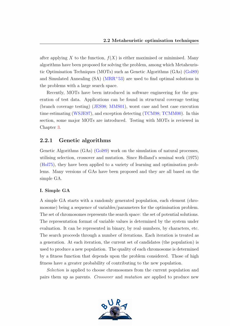
Figure 2.2: The flow chart of simple GA.
26

2.2 Metaheuristic optimisation techniques
chromosomes. A new population is formed from new chromosomes produced on
the basis of crossover and mutation and may also contain chromosomes from the
previous population.
Figure 2.2 shows a flow chart for a simple GA. The following sections give a
detailed explanation on Selection, Crossover and Mutation. All experiments in
this work used roulette wheel selection and uniform crossover.
II. Encoding
In order to apply GAs, a potential solution to a problem should be represented
as a set of parameters. These parameters are joined together to form a string of
values (often referred to as a chromosome). Parameter values can be represented
in various forms such as binary, real-numbers, characters, etc.
Obviously, the encoding strategy is central to the successful application of
GAs. However, at present, there is no theory that enables a rigorous approach
to the selection of the best encoding method for a particular problem. One
principal that an encoding strategy needs to stick to is that the representation
format should make the computation effective and convenient.
III. Reproduction
During the reproductive phase of a GA, individuals are selected from the popu-
lation and recombined, producing children. Parents are selected randomly from
the population using a scheme which favours the more fit individuals. Roulette
Wheel Selection (RWS) and Tournament Selection (TS) are the two most popular
selection regimes that are used for reproduction. RWS involves selecting individ-
uals randomly but weighted as if they were chosen using a roulette wheel, where
the amount of space allocated on the wheel to each individual is proportional to
its fitness, while TS selects the fittest individual from a randomly chosen group
of individuals.
Having selected two parents, their chromosomes are recombined, typically us-
ing the mechanisms of crossover and mutation. Crossover exchanges information
between parent chromosomes by exchanging parameter values to form children.
It takes two individuals, and cuts their chromosome strings at some randomly
27

2.2 Metaheuristic optimisation techniques
Figure 2.3: Crossover operation in simple GA.
28
2.2 Metaheuristic optimisation techniques
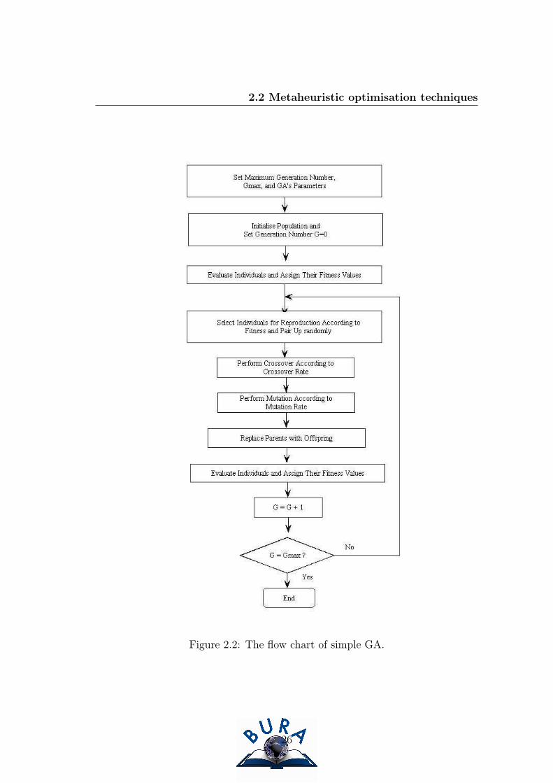
Figure 2.4: Mutation operation in simple GA.
chosen position, to produce two “head” segments, and two “tail” segments. The
tail segments are then swapped over to produce two new full length chromosomes
(see Figure 2.3 – A). Two offspring inherit some genes from each parent. This is
known as single point crossover. In uniform crossover, each gene in the offspring
is created by copying the corresponding gene from one or other parent, chosen
according to a randomly generated crossover mask. Where there is a 1 in the
crossover mask, the gene is copied from the first parent, and where there is a 0
in the mask, the gene is copied from the second parent (see Figure 2.3 – B). The
process is repeated with the parents exchanged to produce the second offspring.
Crossover is not usually applied to all pairs of individuals selected for mating.
A random choice is made, where the likelihood of crossover being applied is
typically between 0.6 and 1.0 (Gol89). If crossover is not applied, offspring are
produced simply by duplicating the parents. This gives each individual a chance
of appearing in the next generation.
Mutation is applied to each child individually after crossover, randomly alter-
ing each gene with a small probability. Figure 2.4 shows the fourth gene of the
chromosome being mutated. Mutation prevents the genetic pool from premature
convergence, namely, getting stuck in local maxima/minima. However, too high
a mutation rate prevents the genetic pool from convergence. A probability value
between 0.01 and 0.1 for mutation is suggested (Gol89).
Elitism might be applied during the evolutionary computation. Elitism in-
29

2.2 Metaheuristic optimisation techniques
volves taking a number of the best individuals through to the next generation
without subjecting them to selection, crossover and mutation. The number of
individuals used for elitism is determined by n(1−G) where n is the population
size and G is the generation gap1.
The use of elitism can significantly improve the performance of a GA for some
problems. However, it should be noted that inappropriate settings for elitism
might lead to premature convergence in the genetic pool.
IV. Sharing Scheme
A simple GA is likely to converge to a single peak, even in domains characterised
by multiple peaks of equivalent fitness. Moreover, in dealing with multimodal
functions with peaks of unequal value, the population of a GA is likely to crowd
to the peak of the highest value. To identify multiple optima in the domain, some
mechanisms should be used to force a GA to maintain a diverse population of
members throughout its search. Sharing is such a mechanism that is proposed
to overcome the above limitations. Sharing, proposed by Holland (Hol75) and
expanded by Goldberg and Richardson (GR87), aims to reduce the fitness of in-
dividuals that have highly similar members within the population. This rewards
individuals that uniquely exploit areas of the domain while discouraging redun-
dant (highly similar) individuals in a domain. This causes population diversity
pressure, which helps maintain population members at local optima.
The shared fitness of an individual i is given by f(sh,i) =f(i)
m(i), where f(i) is
the raw fitness of the individual and m(i) is the peak count. The peak count
is calculated by summing a sharing function over all members of the population
m(i) =∑N
j=i sh(d(i,j)). The distance d(i,j) represents the distance between individ-
ual i and individual j in the population, determined by a similarity measurement.
If the sharing function determines that the distance is within a fixed radius σsh,
it returns a value determined by sh(d(i,j)) = 1− (d(i,j)
σsh)αsh ; otherwise it returns 0.
αsh is a constant that regulates the shape of the sharing function.
1Generation gap is the fraction of individuals replaced in evolving the next generation.
30

2.2 Metaheuristic optimisation techniques
2.2.2 Simulated annealing
Simulated Annealing (SA) was first proposed by Metropolis et al. in 1953. It
was originally proposed as a means of finding the equilibrium configuration of a
collection of atoms at a given temperature. It was Kirkpatrick et al. (KGJV83)
who suggested that a form of simulated annealing could be used for optimisation
problems. The objective for the cooling of a material using a heat bath (a physical
process known as annealing) is to cool the material slowly so that a near perfect
lattice crystal structure (i.e. a state with minimum energy) is obtained. Through
simulating such a process, the aim of simulated annealing is to iteratively improve
a given solution by performing local changes. Changes that improve the solution
are automatically accepted, whereas those changes that make the solution worse
are accepted with a probability that depends on the temperature. Figure 2.5
shows the flow chart of simulated annealing algorithm.
Principally, the process of simulated annealing attempts to avoid local optima
by allowing up-hill (or inferior) solutions in a controlled manner. The idea behind
this is that “it is better to accept a short-term penalty in the hope of finding
significant rewards longer-term” (KGJV83). In accepting an inferior solution,
the search aims to escape from locally optimal solutions in order to find a better
approximation to the global optimum. The control parameter (or temperature) is
used to control the acceptance of inferior solutions. Acceptance of worse solutions
depends upon the degree of inferiority and the current temperature. This degree
is determined by a probability value calculated as e−∆ET where ∆E is the absolute
value of the difference in the objective function values between two solutions and
T is a parameter analogous to the temperature.
The cooling schedule is crucial to the success of the search process. The
selection of the values of iterations and temperatures is considered as using either
a large number of iterations with a small number of temperatures or a small
number of iterations with a larger number of temperatures. Generally, two cooling
schemes are considered (Dow93). In the first case, a geometric reduction of the
temperature by multiplication by a constant α is used. A value between 0.8 and
0.99 is usually suggested for α (KGJV83).
31

2.2 Metaheuristic optimisation techniques
The number of iterations at each temperature in this scheme is usually in-
creased geometrically or arithmetically. This allows intensive search at lower
temperatures to ensure that local optima have been fully explored. An alterna-
tive to geometric increases in iterations is to use feedback from the annealing
process. In this way, the time spent at high temperatures will be small and
the time spent at low temperatures will be large. It is desirable to accept at
least some solutions at each temperature. This aims to ensure that the neigh-
bourhoods have been searched sufficiently. Once the temperature becomes lower,
the number of accepted solutions may become so small that an infeasible num-
ber of iterations are required to accept the desired number of solutions, hence
a maximum limit is normally also imposed. In the second cooling schedule, one
iteration is performed at each temperature. However, the temperature is reduced
extremely slowly in order that the exploration is sufficient. Selection of cooling
schedule with reference to theoretical results of convergence to optimal solutions
has been thoroughly studied by Dowsland (Dow93).
2.2.3 Others
Other MOTs, including hill climbing (RN95) and tabu search, have also been used
for the problems of optimisation. Hill-climbing is essentially an iterative search
where the value of the solution can only increase or stay the same at each step.
In hill climbing, a randomly chosen point and its neighbours are considered for
the search. Once a fitter neighbour is found, it becomes the ‘current point’ in
the search space and the process is repeated; otherwise, if no fitter neighbour is
found, then the search terminates and an optima has been found.
The seminal work on tabu search appears in (Glo89). It is a heuristic search
technique based on the premise that problem solving, in order to qualify as in-
telligent, must incorporate adaptive memory and responsive exploration (Glo89).
Thus, the algorithm of tabu search is based on that of the next k neighbours,
while maintaining a tabu list (memory) that avoids repeating the search in the
same area of the solution space. This is done by means of a tabu list of visited
neighbours that are forbidden. Figure 2.6 illustrates the flow chart of tabu search
algorithm.
32

2.2 Metaheuristic optimisation techniques
Figure 2.5: The flow chart of simulated annealing algorithm.
33

2.2 Metaheuristic optimisation techniques
Figure 2.6: The flow chart of tabu search algorithm.
34

Chapter 3
Test generation - a review
3.1 Introduction
Software needs to be adequately tested in order to ensure (at least to provide con-
fidence) that the implementation under test conforms to its specification. Gener-
ation of test cases is thus required for the purpose of conformance testing. When
testing a system, efficient test cases are always preferred. An efficient test case
should cover all faults that the implementation may have and be relatively short.
Many approaches have been proposed for the generation of test cases. These
approaches are either based upon looking at the program (code) being developed
or rely on examining the specification that the implementation refers to. When
an approach is selected for the generation of test cases, it is often supplemented
by others since no approach guarantees to generate a complete test set. In this
chapter, some of the main test generation techniques are reviewed. Finite state
model based testing techniques are reviewed in chapter 4 separately.
3.2 Adequacy criteria
An adequacy criterion is a criterion that defines what constitutes an adequate
test set. Adequacy criteria are essential to any testing methods as they provide
measurements to justify a test set. Definitions of adequacy criteria might vary
according to different test emphases. Criterion C1 is said to subsume C2 if and
only if whenever a test set satisfies C1, it satisfies C2 as well.
35

3.2 Adequacy criteria
Goodenough et al. (GG75) first studied test criteria and suggested that an
adequacy criterion should be a predicate that defines “what properties of a pro-
gram must be exercised to constitute a ‘thorough’ test, i.e., one whose successful
execution implies no errors in a tested programs”. In order that the correctness
of a program is adequately tested, Goodenough et al. proposed reliability and
validity as properties to justify a test set TS. Reliability requires that a test
criterion always produces consistent test results, while, validity requires that the
test always produces meaningful results, namely, for every error in a program,
there exists a test set that is capable of detecting this error.
Weyuker et al. (WO80) further studied test criteria and pointed out that
these two properties are not independent. Since a criterion must either be valid
or reliable, properties proposed by Goodenough et al. are mutually related.
When measuring a test set, an adequacy criterion can be defined in two ways.
Firstly, an adequacy criterion can be used as a stopping rule to indicate whether
more testing is needed. Secondly, instead of simply stating that a test set is good
or bad, an adequacy criterion can be used to measure test quality by associating
a degree of adequacy with each test set, namely, it not only directs the selection
of test-data, but also decides the sufficiency of a given test set. Currently, two
adequacy uses have been proposed for the evaluation of a test and they are defined
as follows.
Definition 3.2.1 (Test data adequacy criteria as stopping rules) (GG75). A
test data adequacy criterion C is a function C : P × S × T → {true, false}.C(p, s, t) = true means that t is adequate for testing program p against specifica-
tion s according to the criterion C, otherwise t is inadequate.
Definition 3.2.2 (Test data adequacy criteria as measurements) (GG75). A test
data adequacy criterion is a function C, C : P × S × T → [0, 1]. C(p, s, t) = r
means that the adequacy of testing the program p by the test set t with respect to
the specification s is of degree r according to the criterion C. The greater the real
number r, the more adequate the testing.
It can be noted that these two uses are highly related. On one hand, the
stopping rule can be described by the set {false, true} where true suggests that
36

3.3 Black-box and white-box testing
the current test set is adequate enough, while, false implies more testing is re-
quired. The stopping rule can thus be viewed as a special case of measurement;
on the other hand, given an adequacy measurement M and an adequacy degree
d, it is always possible to define a stopping rule Mstop (determined by the test
emphases) such that the adequacy degree dt of a test set is no less than d, dt ≥ d.
In terms of the value of dt, measurement of a test set can be described by the set
{false, true}. In many cases, these two uses are often mutually transformed from
one to the other. By considering the two uses together, the adequacy criterion as
a generator is then defined.
Definition 3.2.3 (Test data adequacy criteria as generator) (BA82). A test data
adequacy criterion C is a function C : P × S → 2T where D is the set of inputs
of the program P and 2T denotes the set of subsets of T . A test set t ∈ C(p, s)
means that t satisfies C with respect to p and s, and it is said that t is adequate
for (p, s) according to C.
3.3 Black-box and white-box testing
Two techniques are widely used in the generation of test cases, these being white-
box testing and black-box testing. In black-box testing, the internal workings of
the item being tested are not known by the tester, while, in white-box testing,
explicit knowledge of the internal workings of the item being tested are used to
select the test data.
It has been suggested that, due to some psychological facts, in the system
development, the designer and the tester should be independent of each other
(Bei90; Boe81). When testing a system, the tester receives very little knowledge
of the internal implementation details of code and often views the system under
test as a ‘black box’. Tests are carried out by using the specification as a reference.
Test cases are generated wholly from the specification, each of which aims to test
some predefined functionalities. That is, given a set of inputs to the system under
test, the only way to justify the correctness of outputs is to compare them to those
defined in the specification. If differences are observed, faults in the system are
then detected. The derivation of test cases in this testing is known as black-box
testing. It is also referred to by some testers as functional testing.
37

3.4 Control flow based testing
One of the advantages of black-box testing is that the test is less likely to be
biased since the designer and the tester are independent of each other. A tester
can conduct the testing from the point of view of the user, not the designer. Test
case design can therefore proceed once the specification is complete.
However, the disadvantages of black box testing can also be noted. If the
tester derives a test case that has already been run by the designer, the test is
redundant. In addition, the test cases are difficult to design. Since it is generally
unrealistic to exhaustively test every possible input stream, some program units
might go untested.
By contrast, it might be possible to look in detail at how test cases actually
exercise particular elements of the implementation, namely, the code. For a given
set of inputs, a program must execute some sequences of small execution steps in
order to calculate the final outputs. Access to information about these steps and
their effects allows more rigorous analysis of what the tests are going to achieve
when the code is executed. This is referred to as white-box testing.
Some of the advantages on white-box testing can be noted. As the knowledge
of internal coding structure is provided, it is easy to find out which type of
input/data can help in testing the application effectively. Meanwhile, by looking
at the internal structure of a program unit, white-box testing may help to optimise
the code.
However, the use of white-box testing may also lead to some disadvantages.
As knowledge of code and internal structure is a prerequisite, a skilled tester is
needed to carry out this type of testing, which increases the cost of testing. At the
same time, it is nearly impossible to look into every bit of code to find out hidden
errors, which might results in the failure of fault detection in an application.
3.4 Control flow based testing
Control-flow based testing is based on the knowledge of the control structure of
the program under test. It is a kind of white box based testing approach. The
control structure of the program is usually represented by a control flow graph
where a syntactic unit such as a predicate in a branch is represented by a node
38

3.4 Control flow based testing
with edges that link this node to the nodes that are reachable through execution.
Figure 3.1 illustrates an example of control flow graph.
Figure 3.1: An example of control flow graph.
In the control flow graph, node nj is called a post-conditioner of ni if, when ni
is executed by an input inputl, nj is reached; ni is called the pre-conditioner of nj.
Two nodes ni and nj in the control flow graph can be merged as one node if and
only if the following condition is satisfied: whenever ni is executed, nj is always a
39

3.4 Control flow based testing
post-conditioner of ni and whenever nj is reached, ni is always a pre-conditioner
of nj. After the control flow graph is accomplished, a path that starts at the first
node (entrance of the program), traverses a sequence of edges and ends up at the
terminal node (end of the program) can then be tested. Such a path is called a
computation path, or an execution path. In order to achieve full testing coverage,
all computation paths in the control flow graph need to be tested.
A variety of coverage criteria can be defined. Here, some major criteria are
described.
Statement coverage
Statement coverage (Nta88; Bei90) reports whether all executable statements in
the program have been encountered. Statement coverage selects a set of test
cases TS such that, by executing a program P with each test case tsi ∈ TS, all
statements of P (nodes in the control graph) have been executed at least once.
The advantage of this measure is that it can be directly applied to object
code and does not require processing source code. However, statement coverage
is subject to a disadvantage where the measurement is insensitive to some control
structures. For example, in the C/C++ code shown in Figure 3.2, without a test
case that causes condition to evaluate false, statement coverage rates this code
fully covered. In fact, if condition ever evaluates false, this code fails.
Figure 3.2: An example of the statement coverage.
Branch coverage
Branch coverage (Nta88) measures the coverage of all blocks and statements that
affect the control flow. In a statement, boolean expressions are evaluated for both
40

3.4 Control flow based testing
true and false conditions. Branch coverage criterion selects a set of test cases TS
such that, by executing a program P with each test case tsi ∈ TS, all edges in
the control graph have been traversed at least once.
It can be noted that branch coverage subsumes statement coverage because
if all edges in a control flow graph are covered, all nodes (statements) are corre-
spondingly covered. Therefore, if a test set satisfies the branch coverage, it also
satisfies the statement coverage.
However, the use of branch coverage may lead to some conditions within
boolean expressions, or relevant combinations of conditions being ignored, which
leads to an incomplete test.
Condition coverage
Condition coverage (Bei90) measures the sub-expressions independently of each
other, which allows for a better analysis of the control flow. Condition coverage
criterion selects a set of test cases TS such that, by executing a program P with
each test case tsi ∈ TS, all edges in the control graph have been traversed at least
once and all possible values of the constituents of compound conditions have been
exercised at least once.
There are two strong versions of condition coverage, these being multiple con-
dition coverage (WHH80) and modified condition/decision coverage (MC/DC)
(CM94). Multiple condition coverage reports whether every possible combina-
tion of boolean sub-expressions has been examined, while, MC/DC requires that
every condition that can affect the result of its encompassing decision needs to
be verified at least once.
With condition coverage, the sub-expressions are combined by logic operator
“AND” and “OR” respectively. Test cases required for full multiple condition
coverage of a condition are given by the logical operator truth table for the
condition. This is how multiple condition coverage works for the generation of
test cases. An advantage of multiple condition coverage is that it requires very
thorough testing, which, in theory, makes it the most desirable structural coverage
measure. However, it may be noted that it is difficult to determine the minimum
set of test cases required to achieve the test goal, especially for those boolean
expressions with high complexity. It has been suggested that, for a decision with
41

3.5 Data flow based testing
n conditions, multiple condition coverage requires 2n tests (WHH80). This makes
the multiple condition an impractical coverage criterion. In addition, the number
of test cases required could vary substantially among conditions that have similar
complexity.
MC/DC was first created at Boeing for the use of testing aviation software.
MC/DC requires that each condition be shown to independently affect the out-
come of the decision. The independence requirement ensures that the effect of
each condition is tested relative to the other conditions. MC/DC is a strong cov-
erage criterion since a thorough execution of the code is required. It subsumes
the branch and statement coverage criteria. However, achieving MC/DC requires
more thoughtful selection of the test cases, and, in general, for a decision with n
conditions, a minimum of n+1 test cases is required (CM94). MC/DC is actually
a mandatory criterion for software developed for critical applications in the civil
aerospace industry (CM94).
Path coverage
Path coverage measures the percentage of all possible paths through the program
being tested. It selects a set of test cases TS such that, by executing a program
P with each test case tsi ∈ TS, all paths starting from the initial node of the
control flow graph of P have been traversed at least once.
It can be noted that, although the path coverage criterion cannot guarantee
program correctness, it is a strong criterion as very thorough testing is required.
The main drawback of the path coverage criterion is that the number of paths
is exponential in the number of branches. Moreover, the number of pathes can
be infinite if a path is a loop. It is also nearly unrealistic to test all possible paths
if the program under test has a large size.
3.5 Data flow based testing
Data-flow based testing (RW85) mainly focuses on the investigation of how values
are associated with variables in a program P and how these associations affect the
execution of the program. In a program, a variable that appears in a statement
42

3.5 Data flow based testing
can be classified as either a definition occurrence or a use occurrence. The defini-
tion occurrence of a variable determines that a value is required to be assigned to
the variable, while, the occurrence of use indicates that the value of the variable
is referred.
A use occurrence of a variable can be classified as two uses - the computational
use and the predicate use. If the value of a variable is used to produce true or false
for a predicate, the occurrence of the variable is called predicate use; otherwise, if
it is used to compute a value for other variables or as an output value, it is called
a computational use. For example, statement y = x1 + x2 requires the values of
x1 and x2 to produce the outcome (definition) of y. In contrast, statement “if
x1 < x2 then goto L endif” contains a predicate that uses the values of x1 and x2
as references.
Three families of adequacy criteria have been proposed for data-flow based
testing. Before introducing these test criteria, some definitions are introduced.
Definition 3.5.1 A variable x is defined if it is declared or assigned to or con-
tained in an input statement.
Definition 3.5.2 A variable x is computation-used if it forms part of the right
hand side of an assignment statement or is used as an index of an array or
contained in an output statement.
Definition 3.5.3 A variable x is predicate-used if it forms part of a predicate in
a conditional-branch statement.
Definition 3.5.4 A definition free path with respect to variable x is a path where
for all nodes in the path there is no definition occurrence of x.
Definition 3.5.5 A path is cycle-free if all visited nodes are distinct.
Lemma 3.5.1 (RW85) A definition occurrence of a variable x at a node u reaches
a computational use occurrence of the variable at node v if and only if there is
a path p from u to v such that p = (u,w1, w2, ..., wn, v), and (w1, w2, ..., wn) is
definition free with respect to x and the occurrence of x at v is a computational
use.
43

3.5 Data flow based testing
Three adequacy criteria
C1: The Rapps-Weyuker-Frankl criteria
Based upon data-flow information, Rapps et al. (RW85) proposed a class of
testing adequacy criteria that mainly focus on the analysis of the simplest type
of data-flow paths that start with a definition of a variable and terminate with a
use of the same variable.
Frankl et al. (FW88) reexamined the criteria and found that the original
definitions of the criteria did not satisfy the applicability property1. They then
modified the definitions and proposed the so-called all-definitions criterion.
Definition 3.5.6 (All-definitions criterion) A set P of execution paths satisfies
the all-definitions criterion if and only if for all definition occurrences of a variable
x such that there is a use of x which is feasibly reachable from the definition,
there is at least one path p in P such that p includes a subpath through which the
definition of x reaches some use occurrence of x.
The all-definition criterion requires that an adequate test set should cover
all definition occurrences in the sense that, for each definition occurrence, the
testing paths should contain a path through which the definition reaches a use of
the definition.
Herman (Her76) studied the data flow information and proposed the all-uses
criterion (also called reach-coverage criterion).
Definition 3.5.7 (All uses criterion) A set P of execution paths satisfies the all-
uses criterion if and only if for all definition occurrences of a variable x and all
uses occurrences of x that the definition feasibly reaches, there is at least one path
p in P such that p includes a subpath through which that definition reaches the
use.
Since one definition occurrence of a variable may reach more than one use oc-
currence, the all-uses criterion requires that all of the uses should be exercised by
testing. This makes the all-uses criterion stronger than the all-definition criterion.
1An adequacy criterion C satisfies the applicability property if and only if for every programP there exists some test set which is C-adequate for P (FW88).
44

3.5 Data flow based testing
A weakness of the above criteria was noticed by Frankl et al. (FW88) and
Clarke et al. (CPR89). Given a definition occurrence of a variable x and a use
of x that is reachable from this definition, there may exist more than one path
through which the definition reaches the use. However, the criteria proposed
above require only one of such paths to be exercised by testing. If all paths are
to be exercised, the testing might be infinite since there may exist infinite such
paths in the flow graph. To overcome this problem, Frankl et al. and Clarke et
al. restricted the paths to be cycle-free or only the end node of the path to be the
same as the start node, and then proposed the all-definition-use-paths criterion.
Definition 3.5.8 (All definition-use-paths criterion) A set P of execution paths
satisfies the all definition-use-paths criterion if and only if for all definitions of a
variable x and all paths q through which that definition reaches a use of x, there is
at least one path p in P such that q is subpath of p, and q is cycle-free or contains
only simple cycles.
C2: The Ntafos required k-tuples criteria
Ntafos (Nta84) studied the interactions among variables from data flow and pro-
posed a class of adequacy criteria called required k-tuples where k > 1 is a nat-
ural number. In the data flow graph, chains of alternating definitions and uses
are called definition-reference interactions (abbreviated as k − dr interactions).
Ntafos’ criteria require a path set that covers the k − dr interactions.
Definition 3.5.9 (Nta88) For k > 1, a k − dr interaction is a sequence K =
[d1(x1), u1(x1), d2(x2), u2(x2), ..., dk(xk), uk(xk)] where
1. di(xi), 1 ≤ i ≤ k, is a definition occurrence of the variable xi;
2. ui(xi), 1 ≤ i ≤ k, is a use occurrence of the variable xi;
3. the use ui(xi) and the definition di+1(xi) are associated with the same node
ni+1;
4. for all i, 1 ≤ i ≤ k. the ith definition di(xi) reaches the ith use ui(xi).
45

3.5 Data flow based testing
Definition 3.5.10 An interaction path for a k − dr interaction is a path p =
((n1) ∗ p1 ∗ (n2) ∗ ... ∗ (nk−1) ∗ pk−1 ∗ (nk)) such that for all i = 1, 2, ..., k− 1, di(xi)
reaches ui(xi) through pi. ni is the node that associates the use ui(xi) with the
definition di+1(xi); pi is a definition-clear path from ni to ni+1.
Clark et al. (CPR89) noted that variables and nodes used in definition 3.5.9
need not be distinct. They then proposed a more useful definition where distinc-
tion of variables and nodes is required.
Definition 3.5.11 (Required k-tuples criteria) A set P of execution paths satis-
fies the required k-tuples criterion, k > 1, if and only if for all j−dr interactions
L, 1 < j ≤ k, there is at least one path p in P such that p includes a subpath
which is an interaction path for L.
C3: The Laski-Korel criteria
Laski and Korel (LK83) studied the data flow and observed that a given node
may contain uses of several different variables, each of which may be reached
by some definitions occurring at different nodes. Such definitions constitute the
computational context of that node. Each node in the flow graph can then be
tested with contexts explored by selecting paths along which the various combi-
nations of definitions that reach the current node. Based upon this observation,
Laski and Korel proposed context coverage criterion.
Definition 3.5.12 (Ordered-context) Let n be a node in the flow graph. Suppose
that there are uses of the variables x1, x2, ..., xm at the node n. Let [n1, n2, ..., nm]
be a sequence of nodes such that for all i = 1, 2, ...,m, there is a definition of xi
on node ni and the definition of xi reaches the node n with respect to xi. A path
p = p1 ∗ (n1)∗p2 ∗ (n2)∗ ...∗pm ∗ (nm)∗pm+1 ∗ (n) is called an ordered context path
for the node n with respect to the sequence [n1, n2, ..., nm] if and only if for all
i = 2, 3, ...,m, the subpath pi ∗ (ni) ∗ pi+1 ∗ (ni+1) ∗ ... ∗ pm+1 is definition free with
respect to xi−1. In this case, the sequence [n1, n2, ..., nm] of nodes is an ordered
context for n.
46

3.6 Partition analysis
Definition 3.5.13 (Ordered-context coverage criterion) A set P of execution
paths satisfies the ordered-context coverage criterion if and only if for all nodes
n and all ordered contexts c for n, there is at least one path p in P such that p
contains a subpath which is an ordered context path for n with respect to c.
Definition 3.5.14 (Context coverage criterion) A set P of execution paths satis-
fies the context coverage criterion if and only if for all nodes n and for all contexts
for n, there is at least one path p in P such that p contains a subpath that is a
definition context path for n with respect to the context.
3.6 Partition analysis
Partition analysis method (OB89) aims to generate a test set that checks pro-
grams on certain error-prone points.
Generally speaking, program errors may fall in two types: computation errors
and domain errors. A computation error is reflected by an incorrect function
in the program. Such an error may be caused, for example, by the execution
of an inappropriate assignment statement that affects the computation outcome
of the function within a path in the program. Domain errors are faults caused
by the incorrect selection of boundaries for a sub-domain. A domain error may
occur, for instance, if a branch predicate is incorrectly expressed, or an assignment
statement that affects a branch predicate is wrong, which will affect the conditions
under which the path is selected.
The partition analysis method works on partitioning the input space into
subdomains and then select a small number of test (usually one) from each of
these subdomains, aiming to find any computation errors in the subdomains.
Each subdomain is defined so that the inputs it contains are treated similarly by
the program, in some sense. It is assumed that this similarity makes it likely that
if the program fails on one input in a subdomain, it also fails on a significant
portion of the others. When testing with partition analysis, in order that the test
effort is reduced, only a few representatives are selected from each subdomain for
testing.
Three strategies have been proposed for the partitions of the input space.
They are discussed in the following.
47

3.6 Partition analysis
3.6.1 Specification based input space partitioning
Specification based input space partitioning considers the use of a subset of data
as a subdomain if the specification requires the same function on the data. An
example of specification based input space partitioning is illustrated in (HH91)
where the function of a module called DISCOUNT INVOICE is described as
follows: Two products, X and Y , are under sales with the single price of $5 for
X and $10 for Y . A discount of 5% will be approved if the total purchasing is
greater than $200. If the total purchasing is greater than $1,000, a discount of
20% is given. Produce X is encouraged for sales where if more than 30 Xs are
purchased, a further discount of 10% is given. In the final calculation, non-integer
costs are rounded down to give an integer value.
DISCOUNT INVOICE module has properties of X ≤ 30 and 5∗X+10∗Y ≤200, and the output is calculated as 5∗X+10∗Y . That is ∀(X, Y ) ∈ {(X, Y )|x ≤30, 5 ∗ X + 10 ∗ Y }, output ≡ 5 ∗ X + 10 ∗ Y . Subset {(X,Y )|x ≤ 30, 5 ∗ X +
10 ∗ Y } should then be treated as one subdomain. In figure 3.3, partition of the
input space of DISCOUNT INVOICE module is illustrated. Six subdomains are
defined.
The above specification is written informally. In most cases, it is hard to
derive partitions from an informal specification. However, if a specification is
written with formal specification languages and the specification is in certain
normal forms, it is always possible to derive partitions.
Hierons (Hie93) proposed a set of transformation rules where specifications
written in pre/postconditions are transformed into the following normal form.
P1(x1, x2, ..., xn) ∧Q1(x1, x2, ..., xn, y1, y2, ..., ym)∨
P2(x1, x2, ..., xn) ∧Q2(x1, x2, ..., xn, y1, y2, ..., ym)∨
...
PK(x1, x2, ..., xn) ∧QK(x1, x2, ..., xn, y1, y2, ..., ym)
where Pi(x1, x2, ..., xn), i = 1, 2, ..., K, are preconditions that give the condition
on the valid input data and the state before the operation, and Qi(x1, x2, ..., xn,
y1, y2, ..., ym), i = 1, 2, ..., K, are post-conditions that specify the relationship
48

3.6 Partition analysis
Figure 3.3: Partition of the input space of DISCOUNT INVOICE module. α, β, γ:borders of the subdomains; a,b,...,h: vertices of the subdomains; A,B,...,F: sub-domains.
between the input data, output data, and the state before and after the operation.
Variables xi are input variables and yi are output variables.
3.6.2 Program based input space partitioning
The input space can be partitioned according to the program structure. In this
type of partitioning, two input data in a subdomain usually execute the same path
in the program. In the program, a path often requires some inputs to trigger the
condition for the execution. The condition is called path condition (How76). A
path condition can be derived by symbolic execution (How76).
For example, in the DISCOUNT INVOICE module, there are six paths in
the program, each of which requires an input to trigger the condition for the
execution of this path. The partitions of input space are therefore determined by
path conditions. Each path in the program is defined as a subdomain.
49

3.6 Partition analysis
Testing with program based partitioning shows some similarities to path cov-
erage based testing. If only one test case is required and the position of the
subdomain is not considered, then testing with program based partitioning is
equivalent to path coverage based testing. However, usually, partitioning test-
ing requires test cases selected not only within the subdomains, but also on the
boundaries, at vertices etc as these points are thought to be error-prone. A test
case in the subdomain is called an on test point; otherwise, an off test point.
3.6.3 Boundary analysis
White et al. (WC80) proposed a test method called N×1 domain-testing strategy
where N test cases need to be selected on the borders in an N−dimensional space
and one case is just off the border. Clarke et al. (CHR82) extended the method
to N × N criterion where, instead of one test case, N test cases are required to
be off the border. Moreover, the N test cases should be linearly independent.
Definition 3.6.1 (N × 1 domain adequacy) (WC80) Let {D1, D2, ..., Dn} be the
set of subdomains of software S that has N input variables. A set T of test cases
is said to be N ×1 domain-test adequate if, for each subdomain Di, i = 1, 2, ..., n,
and each border B of Di, there are at least N test cases on the border B and at
least one test case that is just off B. If the border is in the domain Di, the test
case off the border should be an off test point; otherwise, the test case should be
an on test point.
Definition 3.6.2 (N × N domain adequacy) (CHR82) Let {D1, D2, ..., Dn} be
the set of subdomains of software S that has N input variables. A set T of
test cases is said to be N × N domain-test adequate if, for each subdomain Di,
i = 1, 2, ..., n, and each border B of Di, there are at least N test cases on the
border B and at least N linearly independent test case that is just off B. If the
border is in the domain Di, the N test case off the border should be an off test
point; otherwise, the test case should be an on test point.
It can be seen that boundary analysis focuses on testing the borders of a
subdomain. The N×1 domain-testing strategy aims to check whether there exist
50

3.7 Mutation testing
parallel shift errors in a border, while, N ×N domain-testing strategy checks not
only parallel shift but also rotation of linear borders.
A special case can be noted in boundary analysis, this being vertex testing.
Vertices are intersection points of borders. Clarke et al. (CHR82) suggested
that vertices need to be used as test cases to improve the efficiency of boundary
analysis. She also proposed the adequacy criterion for vertex testing defined as
follows.
Definition 3.6.3 (V × V domain adequacy) (CHR82) Let {D1, D2, ..., Dn} be
the set of subdomains of software S. A set T of test cases is said to be V × V
domain-test adequate if, for each subdomain Di, i = 1, 2, ..., n, T contains the
vertices of Di and for each vertex v of Di, there is a test case just off v. If a
vertex v of Di is in the subdomain Di, then the test case just off v should be an
off test point; otherwise, it should be an on point.
3.7 Mutation testing
Mutation testing (DLS78) is a fault-based testing technique that mainly focuses
on measuring the quality of a test set according to the ability to detect specific
faults. In mutation testing, a number of simple faults, such as simply altered
operators, constant values and variables, are artifactually injected into the pro-
gram under test one at a time. These modified programs are called mutants. A
set of test cases is then designed, aiming to distinguish each mutant from the
original program by the program outputs. If a mutant can be distinguished from
the original program by at least one test case in the test set, the mutant is killed ;
otherwise the mutant is alive.
An example is illustrated in Figure 3.4 where the original code is z = x+y and
two mutants are generated by altering the arithmetic operator “+” to “-” and
“*” respectively. Test case (x = 0, y = 0) kills none of the mutants as the output
z will be the same for the original and mutant programs. Test case (x = 2, y = 2)
kills mutant 1 but fails to kill mutant 2 as, when applying the input, mutant 1
produces an output that is different from that produced by the original program,
while, mutant 2 produces the same output as the original program does. Mutant
1 is then killed while mutant 2 is still alive.
51

3.7 Mutation testing
Figure 3.4: An example of mutation testing.
Mutation testing is based on two assumptions, namely, the competent pro-
grammer hypothesis and the coupling effect (DLS78). The competent program-
mer hypothesis assumes that programmers create programs that are close to being
correct, namely, programmers only make small errors in the programs. This is
the reason why a mutant is generated by deviating the original program slightly
rather then considerably. The coupling effect assumes that a set of test cases that
is capable of finding all simple faults in a program is also able to detect more
complex faults. This assumption assures that the ability of the test set is not
limited to recognising only simple faults.
Sometimes, however, a mutant cannot be killed due to the equivalence of the
mutant and the original program. This leads to the studies of the adequacy of a
test set. The adequacy of a test set is assessed by equation 3.1 where M is the
total number of mutants, D is the number of mutants that has been killed and
E is the number of equivalent mutants.
Adequacy =D
M − E. (3.1)
The problem of deciding whether a mutant is equivalent to the original pro-
gram (determining E in equation 3.1) is generally undecidable. The equivalence
of a mutant is mostly determined manually. More recently, metaheuristic optimi-
sation techniques have been suggested for the elimination of equivalent mutants.
The related work can be found in ref. (AHH04).
One advantage of mutation testing is that it allows a great degree of automa-
tion. Once a set of mutation operators is carefully defined, the generation of
52

3.7 Mutation testing
mutants can be automated. Since the execution of the original program and the
set of generated mutants can be automated, the comparison of the results can be
automated.
However, mutation testing may lead to a high computational cost. It has
been estimated that the number of mutants that can be generated is of the order
of N2 for an N -line program (How82). It might also require expensive human
effort to identify equivalent mutants. Meanwhile, mutation testing relies on two
hypotheses and this might require substantial empirical studies to validate the
correctness of the hypotheses. In addition, mutation testing is still a technique
that largely works on unit test. Instead of being independently used in testing
applications, mutation testing remains a supplement that provides a means to
evaluate the effectiveness of other testing techniques.
Based upon the same idea of mutation analysis, several variants are proposed.
Howden (How82) proposed weak mutation testing to improve the test efficiency.
In the original mutation testing (referred to as strong mutation testing), a change
to a program is made before the execution, and the change is not reversed before
the executions are complete. The outcomes of the original program and the
mutant are compared only when the executions are finished, and the comparison
is made upon the outputs of the two; in weak mutation testing, a component in a
program is mutated. A test set that passes through this component is generated.
If, when applying the test set, the mutated component produces a different value
for a variable than the original one, then this mutant is killed.
The main advantage of weak mutation testing is that it is easier to generate
test cases to kill mutants, which can improve the test efficiency. However, weak
mutation testing only examines the mutated component. This may lead to a
lower level of confidence. Compared to strong mutation testing, weak mutation
testing is inferior.
Woodward et al. (WH88) proposed firm mutation testing. Firm mutation
testing makes a compromise between strong mutation testing and weak mutation
testing. In firm mutation testing, a tester is allowed to make a decision on when
to compare the values between a component and its mutant. It can be set to be
immediately after each single execution of the component, or at some execution
53

3.8 Statistical testing
points in the program. A tester is also allowed to decide how to compare the
outcomes, for example, the output values, or the execution traces, and so on.
Zeil (Zei83) proposed perturbation testing where an “error” space is considered
for the analysis of test effectiveness. Perturbation testing is quite similar to
mutation testing. It is mainly concerned with faults in arithmetic expressions
with program statements. Perturbation testing can be viewed as a special version
of mutation testing.
3.8 Statistical testing
So far, all testing methods discussed are aimed at fault detection, with the goal
of correctness. This, however, is not the only motivation for testing. Given an
extensively tested implementation, if no failure is revealed, it suggests that there
is a higher level of confidence in the system than before the testing is carried
out; otherwise, faults are detected in the system under test. Faults might be
categorised into several types, each of which has some features. If the probability
of a type of fault can be estimated, it would be of great value in improving the
process of testing. Statistical testing is thus proposed to achieve such a goal.
Statistical testing generates test cases using random number generating pro-
cess. When devising a statistical testing strategy, an input space is defined for
test data sampling. The input space defines the set of all possible inputs where
an input defines the set of all variables needed for the calculation of an output.
Test cases must be statistically independent. That is, the next test case chosen
must not be influenced by the history of previously executed tests (Ehr89).
One widely used statistical approach is random testing. It is a form of func-
tional testing. In random testing, test cases are selected randomly from the entire
input domain of the program. When generating a test case, a weight value may
be used to control the distribution of the selected data, for example, uniform
distribution.
The effectiveness of random testing has been studied by several investigators.
However, conclusions drawn from the studies varied significantly. Duran et al.
(DN84) compared random testing with domain partitioning testing and found
that, under the condition where the failure rates in the subdomains were either
54

3.9 Search-based testing
close to 0 or close to 1 and the subdomans are of equal size, the adequacies
of random testing and partitioning testing are close. Miller et al. (MMN+92)
further studied random testing and described circumstances where random testing
can increase confidence. Hamlet et al. (HT90) compared the random testing
with partitioning testing by considering boundary cases where there exist hidden
subdomains, subdomains that random testing is less likely to hit, and found that
partitioning testing is far better than random testing. This study suggests that
the effectiveness of partitioning testing and random testing is heavily affected by
the expected failure rates of boundary cases.
The principal advantage of random testing is that it is comparatively simple
and involves little effort in the generation of test cases. When automating the
process of random testing, the use of a test oracle is usually not a requirement.
In addition, random testing provides supplements for other testing techniques.
As introduced in the previous chapters, testing is a complicated process and no
testing technique guarantees to generate a complete test. Random testing can be
used to further measure the adequacy of other techniques.
One of the big problems of random testing is when to stop testing. The other
problem of random testing is to know when a test fails (DN84). It is hard to
determine if the test cases generated with random testing has completely tested
the system under test. To overcome these drawbacks, it is advisable to use some
other techniques to check the adequacy of these test sets.
3.9 Search-based testing
Search based optimisation techniques such as Genetic Algorithms (GAs) and
Simulated Annealing (SA) (see chapter 2) have recently been applied in the gen-
eration of test cases. In order that search based techniques can be applied, an
objective fobj function is required to evaluate the quality of a test case. A set of
test cases is iteratively updated to explore the test cases that maximise/minimise
fobj.
The reasons that search based techniques are used in the generation of test
cases are: (1) the problem of generating test cases is equivalent to a search
problem where good solutions need to be explored in the input space of the
55

3.9 Search-based testing
system being developed. Usually, the input space has a large size. This could
make the search a costly and inefficient process when traditional algorithms are
applied. This problem, however, can be alleviated by heuristic search; (2) some
problems in testing are NP-hard and search based techniques have proved efficient
in providing good solutions for NP-problems.
Jones et al. (JES98) applied GAs for structural coverage testing (branch
coverage testing). In the work, the control flow of the program is created. A
fitness function is defined to guide the search of test data. This fitness function is
based on the predicate associated with each branch, and a value for fitness derived
from either a Hamming distance or a simple numerical reciprocal function. The
simulation results suggested the test data generated are of high quality. Michael
et al. (MMS01) studied the automated generation of dynamic test data by using
GAs. A tool called GADGET (the Genetic Algorithm Data GEneration Tool)
was devised for exploring test data. This tool allows the test generator to slightly
modify the input parameters of the program, attempting to lead them to the
values that satisfy the test requirement.
Tracey et al. (TCM98; TCMM00) investigated exception detection using GAs
and SA respectively. Exception is a sub-class of failures. It might be caused by
incorrect inputs, hardware faults or logical errors in the software code. In the
work, a fitness function (see table 3.1) is defined to justify the test data that
might raise exceptions. This fitness function provides a measure of how close a
test case is to execute a desired raise statement. The process of the generation of
such test data is further optimised by using GAs. The experimental results show
the effectiveness of the proposed method.
Wegner et al. (WSJE97) investigated worst case and best case execution
time estimation by using GAs. In the work, based upon the execution time
measured in processor cycles, a fitness function is defined. A number of programs
are used for experiments. By checking the experimental results, Wegner et al.
claimed that GAs are able to check large programs. At the same time, they show
considerable promise in establishing the validity of the temporal behaviour of
real-time software.
However, the use of search based techniques for the generation of test cases has
some limitations as well. Usually, in search based testing, inputs of the program
56

3.9 Search-based testing
Element ValueBoolean if TRUE then 0 else Ka = b if abs(a− b) = 0 then 0
else abs(a− b) +Ka 6= b if abs(a− b) 6= 0 then 0
else Ka < b if a− b < 0 then 0
else (a− b) +Ka ≤ b if a− b ≤ 0 then 0
else (a− b) +Ka > b if b− a < 0 then 0
else (b− a) +Ka ≥ b if b− a ≤ 0 then 0
else (b− 1) +Ka ∨ b min(fit(a), fit(b))a ∧ b fit(a) + fit(b)−a Negation is moved inwards and propagated over a
Table 3.1: Fitness function cited from (TCMM00).
constitute the search space. Search based techniques iteratively construct a set
of test cases from such a space, attempting to maximise/minimise a predefined
objective function. In most cases, the landscape of the input space is not known.
This makes it very difficult to determine when to stop the search for the test
data.
Currently, two rules are applied for terminating the computation. In the
first case, a comparatively large number of iterations is defined, which leads to
a saturated computation. However, if the computation converges at a very early
stage, this termination rule will result in redundant computation. For example,
if a predefined number of iterations is 1000 and the computation converges in
100 iterations, the rest of the computation contributes no effort in improving the
quality of test data and becomes redundant. The other rule is to define a time pe-
riod. If the performance of the exploration has no significant improvement within
such a period, it is assumed that the maximum/minimum value is reached and
the computation is terminated. This, however, can also lead to some problems.
If the computation gets stuck in a local optimal within such a period, the process
57

3.9 Search-based testing
of search is terminated and the final result obtained is not globally optimal.
58

Chapter 4
Testing from finite state machines
4.1 Introduction
Finite state machines are formal specification languages. Since being developed,
finite state machines have been used for modelling systems in various areas such as
sequential circuits (Moo56; Hen64; KK68; Hsi71), software engineering (Cho78)
and communication protocols (ATLU91; MP93; Hie96; SLD92; YU90).
In system development, a system is often modelled as a set of functional
units or components. Some of these units are connected with others through
input/output coupling. Each unit in the system is assigned with two attributes:
an I/O port and an internal state. I/O port provides developers with an interface
for the output observation when an input is sent while the internal state is not
observable and can only be inferred from exhibited I/O behaviour.
Finite state machines, which involve a finite number of states and transi-
tions between these states, are suitable for describing and implementing the con-
trol logic for applications. Compared to the other specification languages, finite
state machines have several advantages: (1) they are comparatively simple, which
makes it easy for inexperienced developers to implement; (2) in deterministic fi-
nite state machines, given a set of inputs and a known current state, the terminal
state is predictable. The predicability of finite state machines helps to reduce
the complexity of testing; (3) as a finite state machine can be represented by a
directed graph, techniques involving directed graph theory can be applied with
little modification; and (4) finite state machines have been studied for many years
59

4.2 Finite state machines
and become mature techniques for system modelling and testing.
Finite state machines have been considered as a useful way for automating
the process of test generation from the system being developed. In finite state
machine based testing, a test design is usually accomplished in two steps:
1. define a test strategy for the test objects;
2. automate the process of generating test sequences.
Test objects refer to all transitions contained in the finite state machine un-
der test. A standard test strategy usually tests a transition in two parts: I/O
behaviour check and the final state verification. Details about the standard test
strategy are discussed in section 4.3. A complete testing sequence guarantees
that all transitions contained in the finite state machine have been adequately
tested. In the test process, it is usually preferred that a test sequence will con-
tinuously test all transitions without being mandatorily halted (say, manually
reset). In section 4.4, the process that controls the generation of test sequences
is introduced and in section 4.5, minimisation on the length of a test sequence is
discussed.
4.2 Finite state machines
Definition 4.2.1 A finite state machine (FSM) M is defined as a 5-tuple
M = (I, O, S, δ, λ, s0)
where I, O, and S are finite and nonempty sets of input symbols, output symbols,
and states, respectively; δ : S × I → S is the state transition function; and
λ : S × I → O is the output function. s0 is the initial state of the machine.
In an FSM, if the machine receives an input a ∈ I when in state si ∈ S,
it moves to the state si+1 = δ(si, a) and produces output λ(si, a). Functions
δ and λ can be extended to take input sequences in the usual way. An input
sequence x = a1a2...ak takes the machine from a start state sl successively to
state si+1 = δ(si, ai), i = l, ..., k, with the final state sk+1 = δ(sl, x), and produces
an output sequence b1, ..., bk = λ(sl, x) where bi = λ(si, ai), i = l, ..., k.
60

4.2 Finite state machines
Figure 4.1: Finite state machine represented by digraph cited from ref.(ATLU91).
61

4.2 Finite state machines
a b cs1 s1, x s2, x s4, ys2 s5, x s3, y Nones3 None s5, x s5, ys4 s5, x s3, x Nones5 s4, z None s1,z
Table 4.1: Finite state machine represented by state table.
An FSM M can be represented by a labelled directed graph D = (V,E),
where the set of vertices V represents the state set S of M and the set of edges
E represents the transitions. An edge has label a/o where a ∈ I and o ∈ O
are the corresponding transition’s input and output. Figure 4.1 (copied from ref.
(ATLU91)) illustrates an FSM represented by its corresponding directed graph.
Alternatively, an FSM can be represented by a state table where one row lists
each state and one column is used for each input. Table 4.1 shows the state table
of the above FSM.
An FSM is deterministic if and only if for any state si ∈ S and an input a ∈ Ithere is at most one transition involving si and a. Two states si and sj of M are
said to be equivalent if and only if for every input sequence α ∈ I the machine
produces the same output sequence, λ(si, α) = λ(sj, α). Machines M1 and M2
are equivalent if and only if for every state in M1 there is an equivalent state in
M2, and vice versa. A machine M is minimal (reduced) if and only if no FSM
with fewer states than M is equivalent to M .
It is assumed that any FSM being considered is minimal since any (deter-
ministic) FSM can be converted into an equivalent (deterministic) minimal FSM
(LY96). An FSM is completely specified if and only if for each state si and input a,
there is a specified next state si+1 = δ(si, a), and a specified output oi = λ(si, a);
otherwise, the machine is partially specified.
A partially specified FSM can be converted to a completely specified one in
two ways (LY96). One way is to define an error state. When a machine is in
state s and receives an input a such that there is no transition from s with input
a, it moves to the error state with a given (error) output. The other way is to
add a loop transition. When receiving an undefined input, the state of a machine
62

4.3 Conformance testing
remains unchanged. At the same time, the machine produces no output. An
FSM is strongly connected if the underlying directed graph is strongly connected.
It is assumed throughout this thesis that finite state machines under test are
deterministic, minimal, completely specified and strongly connected.
4.3 Conformance testing
Given a specification FSM M , for which we have its complete transition diagram,
and an implementation M ′, for which we can only observe its I/O behaviour
(“black box testing”), we want to test to determine whether the I/O behaviour
of M ′ conforms to that of M . This is called conformance testing. A test sequence
that solves this problem is called a checking sequence.
An I/O difference between the specification and implementation can be caused
by either an incorrect output (an output fault) or an earlier incorrect state transfer
(a state transfer fault). Hennie (Hen64) suggests that the latter can be detected
by adding a final state check after a transition check is finished. In Hennie’s
work, a test procedure is split into two parts, namely, I/O check and tail state
verification. This contributes to the current standard test strategy. A standard
test strategy is:
1. Homing: Move M ′ to an initial state s;
2. Output Check: Apply an input sequence α and compare the output se-
quences generated by M and M ′ separately;
3. Tail State Verification: Using state verification techniques to check the final
state.
It is assumed throughout this thesis that all test sequences are generated using
the standard test strategy.
The first step in the test is known as homing a machine to a desired initial
state. This can be accomplished by using a homing sequence or a synchronizing
sequence.
Definition 4.3.1 A homing sequence H is an input sequence such that the output
sequence on H uniquely determines the state reached after applying H.
63

4.3 Conformance testing
Definition 4.3.2 A synchronizing sequence SN is an input sequence that moves
the FSM to some fixed state irrespective of the initial state.
Moore (Moo56) proved that all FSMs have homing sequences. However, not
all FSMs have a synchronizing sequence. Kohavi (Koh78) proved that, if an
FSM has a synchronizing sequence, the length of the sequence does not exceed
n(n−1)(n+1)/6 where n is the number of states in the FSM. However, in his work,
no algorithm is proposed for the construction of a synchronizing sequence. In case
there exists no synchronizing sequence, an adaptive synchronizing experiment can
be considered to move the FSM to a desired state.
Definition 4.3.3 An adaptive synchronizing experiment is a strategy that will
place the FSM in a particular state but with the input values used depending upon
the previous output.
Obviously, an adaptive synchronizing experiment is feasible in every strongly
connected finite state machine as it is sufficient to execute a homing sequence to
move the machine to a known state and then apply a transfer sequence to move
the FSM to the desired state.
The second step in the test checks whether M ′ produces the desired output
sequence. A fault detected at this stage is called an output fault. The last step
checks whether M ′ is in the expected state s′ = δ(s, α) after the transition. A
fault detected at this stage is called a state transfer fault. There are three main
techniques used for state verification:
• Distinguishing Sequence (DS)
• Unique Input/Output (UIO)
• Characterizing Set (CS)
Definition 4.3.4 A distinguishing sequence is an input sequence that produces a
different output for each state.
Execution of a DS provides evidence of the state an FSM is in when the DS
is input. However, not every FSM has a DS (LY94).
64

4.3 Conformance testing
Definition 4.3.5 A UIO sequence of state si is an input/output sequence x/y,
that may be observed from si, such that the output sequence produced by the ma-
chine in response to x from any other state is different from y, i.e. λ(si, x) = y
and λ(si, x) 6= λ(sj, x) for any i 6= j.
A DS defines a UIO sequence for every state. While not every FSM has a
UIO for each state, some FSMs without a DS have a UIO for each state.
Definition 4.3.6 A characterizing set W is a set of input sequences with the
property that, for every pair of state (si, sj), j 6= i, there is some w ∈ W such
that λ(si, w) 6= λ(sj, w). Thus, the output sequences produced by executing each
w ∈ W from sj verifies sj.
The uses of DS, CS and UIO for state verification are proposed by Hennie
(1964) (Hen64), Chow (1978) (Cho78) and Chen et al. (1989) (CVI89) separately.
Compared to the other two techniques, the use of UIOs has several advantages:
(1) Not all FSMs have a Distinguishing Sequence (DS), but nearly all FSMs have
UIOs for each state (LY94); (2) The length of a UIO is no longer than that of
a DS; (3) While UIOs may be longer than a characterizing set, in practice UIOs
often lead to shorter test sequences.
However, computing a DS or UIOs from an FSM is NP-complete (LY94).
Lee et al. (LY94) note that adaptive distinguishing sequences and UIOs may be
produced by constructing a state splitting tree from the FSM being investigated.
A State Splitting Tree (SST) is a rooted tree T that is used to construct
adaptive distinguishing sequences or UIOs from an FSM. Each node in the tree
has a predecessor (parent) and successors (children). A tree starts from a root
node and terminates at discrete partitions: sets that contain one state only. The
predecessor of the root node, which contains the set of all states, is null. The
nodes corresponding to a single state have empty successor. These nodes are
also known as terminals. A child node is connected to its parent node through
an edge labelled with characters. The edge implies that the set of states in the
child node is partitioned from that in the parent node upon receiving the labelled
characters. The splitting tree is complete if the partition is a discrete partition.
65

4.3 Conformance testing
Figure 4.2: A pattern of state splitting tree from an FSM.
66

4.3 Conformance testing
An example is illustrated in Figure 4.2 where an FSM (different from the
one shown in Figure 4.1) has six states, namely, S = {s1, s2, s3, s4, s5, s6}. The
input set is I = {a, b} while the output set is O = {x, y}. The root node is
indicated by N(0, 0)1, containing the set of all states. Suppose states {s1, s3, s5}produce x when responding to a, while {s2, s4, s6} produce y. Then {s1, s3, s5}and {s2, s4, s6} are distinguished by a. Two new nodes rooted from N(0, 0) are
then generated, indicated by N(1, 1) and N(1, 2). If we then apply b, the state
reached from {s1} by a produces x while the states reached from {s3, s5} by a
produce y. Thus ab distinguish {s1} from {s3, s5}. Two new nodes rooted from
N(1, 1) are generated, denoted byN(2, 1) andN(2, 2). The same operation can be
applied to {s2, s4, s6}. Repeating this process, we can get all discrete partitions
as shown in Figure 2. Note that for some FSMs this process might terminate
without producing a complete set of discrete partitions since there need not exist
such a tree (LY96). A path from a discrete partition node to the root node forms
a UIO for the state related to this node. When the splitting tree is complete, we
can construct UIOs for each state.
Unfortunately, the problem of finding data to build up the state splitting tree
is NP-hard. This provides the motivation for this PhD work, which investigates
the use of MOTs for the construction of UIOs. The problem is discussed in
chapter 5.
Shen et al. (SST91) shows that using a backward UIO (B-UIO) in a transition
test helps to improve test quality. By applying a B-UIO, the initial state of the
transition is also verified. All states in B-UIO method are verified twice. The
test quality is therefore improved.
Definition 4.3.7 A Backward UIO (B-UIO) sequence of state si is an input/output
sequence x/y, that can be observed only if the final state of transitions is si, i.e.
∀sj (sj ∈ S), λ(sj, x) = y ⇒ δ(sj, x) = si.
When both UIOs (forward) and B-UIOs are considered, the method is called
the B-UIO method, or simply B-method. The test strategy is then:
1N(i, j): i indicates that the node is in the ith layer from the tree. j refers to the jth nodein the ith layer.
67

4.4 Test sequence generation
1. Homing: Move M ′ to the initial state of the B-UIO;
2. Initial state verification: Apply the B-UIO sequence to move M ′ to the
initial state of a transition;
3. Output check: Apply an input α and compare the outputs generated by M
and M ′ separately;
4. Tail state verification: Apply UIO (forward) to check the final state.
The UIO (forward) is used to provide confidence that the tested transition arrives
at a correct state while the Backward UIO is used to increase the confidence that
an assigned transition has been tested.
4.4 Test sequence generation
When testing from FSMs, it is always desirable that a test sequence will detect
all faults from the Implementation Under Test (IUT) with the shortest length.
In finite state machine based testing, testing is performed in “black-box” man-
ner. Thus, the number of states in the IUT is not known. This requires some
assumptions before testing starts.
It has been shown that, if the number of states in the IUT exceeds the num-
ber of states in its specification, the process of conformance testing is NP-hard
(Moo56). Moore (Moo56) proved that, given a minimal FSM M and a faulty
implementation M′, it is always possible to generate an input sequence that will
distinguish M′from M as long as M
′has no more states than M . Based upon
Moore’s work, four test methods are proposed for the generation of test sequences
from the FSM under test. They are T-method (NT81), D-method (Hen64), W-
method (Cho78) and U-method (CVI89). T-, D- and U-methods assume that
the number of states in the IUT does not exceed that in the specification FSM.
W-method allows more states in the IUT but assumes that the maximum number
of states that the correct design might have is known.
In the T-method, a test sequence (called a transition-tour sequence) is gen-
erated simply by applying inputs to the specification FSM until all transitions
in the FSM have been traversed at least once. In the D-, W-, and U-methods,
68
4.5 Optimisation on the length of test sequences
as well as each transition being executed, tail state of the transition needs to be
verified by DS, CS, and UIO correspondingly. D-, W-, and U-methods are called
formal methods. In terms of fault coverage, D-, W-, and U-methods outperform
T-method (SL89).
A method for generating a complete test sequence is described as follows: an
untested transition is selected from the specification FSM first. The FSM is then
moved to the initial state of the selected transition by using a transfer sequence.
This transfer sequence is also called a linking sequence in the final test sequence.
Normally, the test process starts with a transition whose starting state is the
initial state of the FSM where no transferring operation is required. The selected
transition is then tested by checking its I/O plus verifying the tail state. An
input sequence that will test the selected transition is called the test sequence for
this transition.
After a test is complete, another transition is selected. The FSM is then
moved to the initial state of the selected transition by a transfer sequence. The
process of transition testing starts and the selected transition is tested by its test
sequence. The process repeats until all transitions have been adequately tested.
However, test sequence generated by such a process might result in a long
sequence, which consequently increases the cost in the forthcoming implementa-
tion test. A short test sequence is thus preferred. This leads to the problem of
minimisation on the length of a test sequence.
Clearly, the increment of a test sequence’s length is caused by the uses of
linking sequences. If, when generating a test sequence, a set of linking sequences
is applied such that the sum of the length of all linking sequences is minimal,
the test sequence is of the minimal length. In the next section, techniques for
generating an optimal test sequence from an FSM are discussed.
4.5 Optimisation on the length of test sequences
4.5.1 Single UIO based optimisation
Aho et al. (ATLU91) noted that an optimal test sequence may be produced when
UIOs are used for state verification. In their work, Aho et al. proved that, if an
69

4.5 Optimisation on the length of test sequences
FSM M is strongly connected or weakly connected with all states having reset
functions, there exists a Chinese postman tour T in the test control digraph of M .
Inputs derived from T constitute an optimal test sequence for M . Based upon
rural Chinese postman tour algorithm, an optimal technique for the generation of
a test sequence from the FSM under test is proposed. This technique is described
as follows.
Let us suppose that we have a specification FSM M with the input set I
and the output set O respectively. The FSM is represented by a digraph D =
(V,E) where V represents the set of states and E the set of transitions. Let
(vi, vj, am/on) ∈ E be a transition under test where vi is the initial state and vj
the final state. am/on is the I/O pair of this transition, am ∈ I, on ∈ O. Let UIOj
be the UIO sequence for vj. When in vj and receiving the input part of UIOj,
M produces the output part of UIOj and arrives at vk. The final state of UIOsj
is denoted as vk = Tail(UIOj). The test sequence for a transition (vi, vj, am/on)
is constructed by concatenating am with the input part of UIOj. After the test
of (vi, vj, am/on) is complete, a test control trail1 for the transition is produced,
denoted as 2(vi, vk; (am/on) · UIOj), Tail(UIOj) = vk. If all transitions in M
have been tested by their test sequences, we can finally get a complete set of test
control trails. This set is denoted as:
EC = {(vi, vk; (am/on) · UIOj) : (vi, vj; am/on) ∈ E ∧ Tail(UIOj) = vk}.
A digraph D′
= (V′, E
′) is then constructed such that V
′ ≡ V and E′
=
EC ∪E. Digraph D′is called the test control digraph of D. It is easy to see that
if an input sequence traverses all edges in D′at least once, then all transitions
in D (or more precisely M) are tested at least once. The problem of generating
an optimal test sequence from D is now converted to that of finding the Chinese
postman tour in D′. As introduced in chapter 2, if D
′is symmetric, there exists
an Euler tour in D′and the Euler tour is also a Chinese postman tour; otherwise,
1A test control trail implies the sequence of transitions that the machine will traverse whena transition is tested by its test sequence. Here, only the initial state of the first transition andthe final state of the last transition are drawn.
2The notation ‘·’ indicates the concatenation of two sequences.
70

4.5 Optimisation on the length of test sequences
State UIO Final Statev1 ba/xx v5
v2 b/y v3
v3 bc/xz v1
v4 bc/xy v5
v5 c/z v1
Table 4.2: UIO sequences for the states of the FSM shown in fig.4.1.
D′
needs to be augmented to derive its symmetric augmentation digraph D∗.
Once D∗ is complete, the Euler tour in D∗ is equivalent to the Chinese postman
tour in D′. When augmenting D
′, the cost of an edge in D
′is calculated as:
C(vi, vk; (am/on) · UIOj) = C(vi, vj; (am/on)) + C(UIOj).
A flow network is thus required for calculating the replication times ψ(vi, vj; am/on)
for a transition (vi, vj; am/on) ∈ E.
To further explain the control scheme, an example is illustrated where the
FSM shown in Figure 4.1 is utilised. The UIOs for states are listed in table
4.2. We also allow the FSM to have a reset function ri. When receiving ri, the
machine returns to v1 and produces null, regardless of the current state.
In order to generate the test control digraph D′for the FSM, each transition’s
test control trail needs to be derived. For example, the test control trail for
transition (s1, s1; a/x) is constructed by (v1, v5; (a/x) · (ba/xx)), Tail(UIO1) =
Tail(ba/xx) = v5. An edge starting with v1, ending with v5 and labelled with
aba/xxx is added to digraph D′. The test cost for this edge is calculated as
C(v1, v5; (a/x) · (ba/xx)) = C(v1, v1; a/x) + C(v1, v5; ba/xx).
Let the cost of an edge in the FSM be 1. Test cost of edge (v1, v5; (a/x) ·(ba/xx)), Tail(UIO1) = Tail(ba/xx) = v5 is then 3. There are 11 transitions
in the FSM. All transition’s test control trails need to be added to D′. Test
control trails of all transitions are listed in table 4.3. Five additional test control
trails that are related to reset function are also included in the final test control
digraph. The final test control digraph generated from table 4.3 and Figure 4.1
is shown in Figure 4.3.
71

4.5 Optimisation on the length of test sequences
Figure 4.3: Test control digraph of the FSM shown in fig. 4.1 using single UIOfor each state.
72

4.5 Optimisation on the length of test sequences
No Transition Tail state verification Test control trail1 (v1, v1; a/x) (v1, v5; ba/xx) (v1, v5; aba/xxx)2 (v1, v4; c/y) (v4, v5; bc/xy) (v1, v5; cbc/yxy)3 (v1, v2; b/x) (v2, v3; b/y) (v1, v3; bb/xy)4 (v2, v3; b/y) (v3, vs1; bc/xz) (v2, v1; bbc/yxz)5 (v2, v5; a/x) (v5, v1; c/z) (v2, v1; ac/xz)6 (v3, v5; b/x) (v5, v1; c/z) (v3, v1; bc/xz)7 (v3, v5; c/y) (v5, v1; c/z) (v3, v1; cc/yz)8 (v4, v3; b/x) (v3, v1; bc/xz) (v4, v1; bbc/xxz)9 (v4, v5; a/x) (v5, v1; c/z) (v4, v1; ac/xz)10 (v5, v1; c/z) (v1, v5; ba/xx) (v5, v5; cba/zxx)11 (v5, v4; a/z) (v4, v5; bc/xy) (v5, v5; abc/zxy)12 (v1, v1; ri/null) (v1, v5; ba/xx) (v1, v5; (ri/null)(ba/xx))13 (v2, v1; ri/null) (v1, v5; ba/xx) (v2, v5; (ri/null)(ba/xx))14 (v3, v1; ri/null) (v1, v5; ba/xx) (v3, v5; (ri/null)(ba/xx))15 (v4, v1; ri/null) (v1, v5; ba/xx) (v4, v5; (ri/null)(ba/xx))16 (v5, v1; ri/null) (v1, v5; ba/xx) (v5, v5; (ri/null)(ba/xx))
Table 4.3: Test control trails of transitions in the FSM shown in fig. 4.1.
The problem now comes to finding the Chinese postman tour in D′. As
one can see D′is not symmetric and therefore does not contain an Euler tour.
The symmetric augmentation of D′
is thus required. In order to construct the
symmetric augmentation digraph D∗ of D′, a flow network DF = (VF , EF ) needs
to be constructed. DF is defined as VF = V (D′)∪{s, t} where s is the source and
t the sink, and EF = E(D) ∪E+ ∪E− where E+ = {(s, v1), (s, v5)}, u(s, v1) = 2,1u(s, v5) = 6; E− = {(v2, t), (v3, t), (v4, t)}, u(v2, t) = 3, u(v3, t) = 2, u(v4, t) = 3.
E+ and E− are derived through calculating the index of each vertex (state),
ξ(vi) = d−vi− d+
vi. Edges in E+ and E− have zero test cost. The capacity of these
edges are defined as u(vi, s) = ξ(vi), u(t, vj) = −ξ(vj). The rest of the edges in
E′have the same cost as those edges in E and have infinite capacities (for more
details, see chapter 2).
Thus, in terms of a max flow F , a function ψ(vi, vj; am/on) is required to
determine the times of replication for the edge (vi, vj) ∈ E in D∗. The function
1u(s, vi) defines the capacity of edge (s, vi).
73

4.5 Optimisation on the length of test sequences
Figure 4.4: The flow graph DF of the digraph D′with the maximum flow and
minimum cost.
is defined as:
ψ(vi, vj; am/on) =
{1, if (vi, vj; am/on) ∈ EC
F (vi, vj; am/on), if (vi, vj; am/on) ∈ E
Finding a maximum-flow/minimum-cost flow F on DF over ψ leads to a sym-
metric augmentation D∗ of D′(ATLU91). F gives us ψ which defines the times
of replication of edge (vi, vj) in D∗. The final flow in the network is shown in
Figure 4.4. The number on each edge indicates the times that this edge needs to
be replicated.
Having replicated edges in D′
by the times given in DF , a symmetric aug-
mentation digraph D∗ is generated shown in Figure 4.5. An Euler tour can then
be constructed from D∗ by using the algorithm proposed by (Kua62). This Euler
tour is also a Chinese postman tour in D′. Test sequence derived from this tour
is an optimal test sequence for the FSM shown in Figure 4.1. The result is shown
in table 4.4. There are total 55 input/output pairs.
74

4.5 Optimisation on the length of test sequences
Figure 4.5: Symmetric augmentation from fig. 4.3. Number in an edge indicatesthe times this edge needs to be replicated.
ri/null bb/xy cc/yz aba/xxxabc/zxy cba/zxx (ri/null) · (ba/xx) a/xac/xz cbc/yxy a/z b/xbc/cz b/x bbc/yxz b/xac/xz b/x (ri/null) · (ba/xx) a/zb/x (ri/null) · (ba/xx) a/z bbc/xxz
(ri/null) · (ba/xx) a/z (ri/null) · (ba/xx) c/z
Table 4.4: An optimal test sequence for the FSM shown in fig. 4.1 by using singleUIO for each state.
75
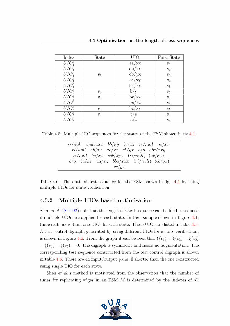
4.5 Optimisation on the length of test sequences
Index State UIO Final StateUIO1
1 aa/xx v1
UIO21 ab/xx v2
UIO31 v1 cb/yx v3
UIO41 ac/xy v4
UIO51 ba/xx v5
UIO12 v2 b/y v3
UIO13 v3 bc/xz v1
UIO23 ba/xz v4
UIO14 v4 bc/xy v5
UIO15 v5 c/z v1
UIO25 a/z v4
Table 4.5: Multiple UIO sequences for the states of the FSM shown in fig.4.1.
ri/null aaa/xxx bb/xy bc/xz ri/null ab/xxri/null ab/xx ac/xz cb/yx c/y abc/zxyri/null ba/xx ccb/zyx (ri/null) · (ab/xx)
b/y ba/xz aa/xz bba/xxx (ri/null) · (cb/yx)cc/yz
Table 4.6: The optimal test sequence for the FSM shown in fig. 4.1 by usingmultiple UIOs for state verification.
4.5.2 Multiple UIOs based optimisation
Shen et al. (SLD92) note that the length of a test sequence can be further reduced
if multiple UIOs are applied for each state. In the example shown in Figure 4.1,
there exits more than one UIOs for each state. These UIOs are listed in table 4.5.
A test control digraph, generated by using different UIOs for a state verification,
is shown in Figure 4.6. From the graph it can be seen that ξ(v1) = ξ(v2) = ξ(v3)
= ξ(v4) = ξ(v5) = 0. The digraph is symmetric and needs no augmentation. The
corresponding test sequence constructed from the test control digraph is shown
in table 4.6. There are 44 input/output pairs, ll shorter than the one constructed
using single UIO for each state.
Shen et al.’s method is motivated from the observation that the number of
times for replicating edges in an FSM M is determined by the indexes of all
76
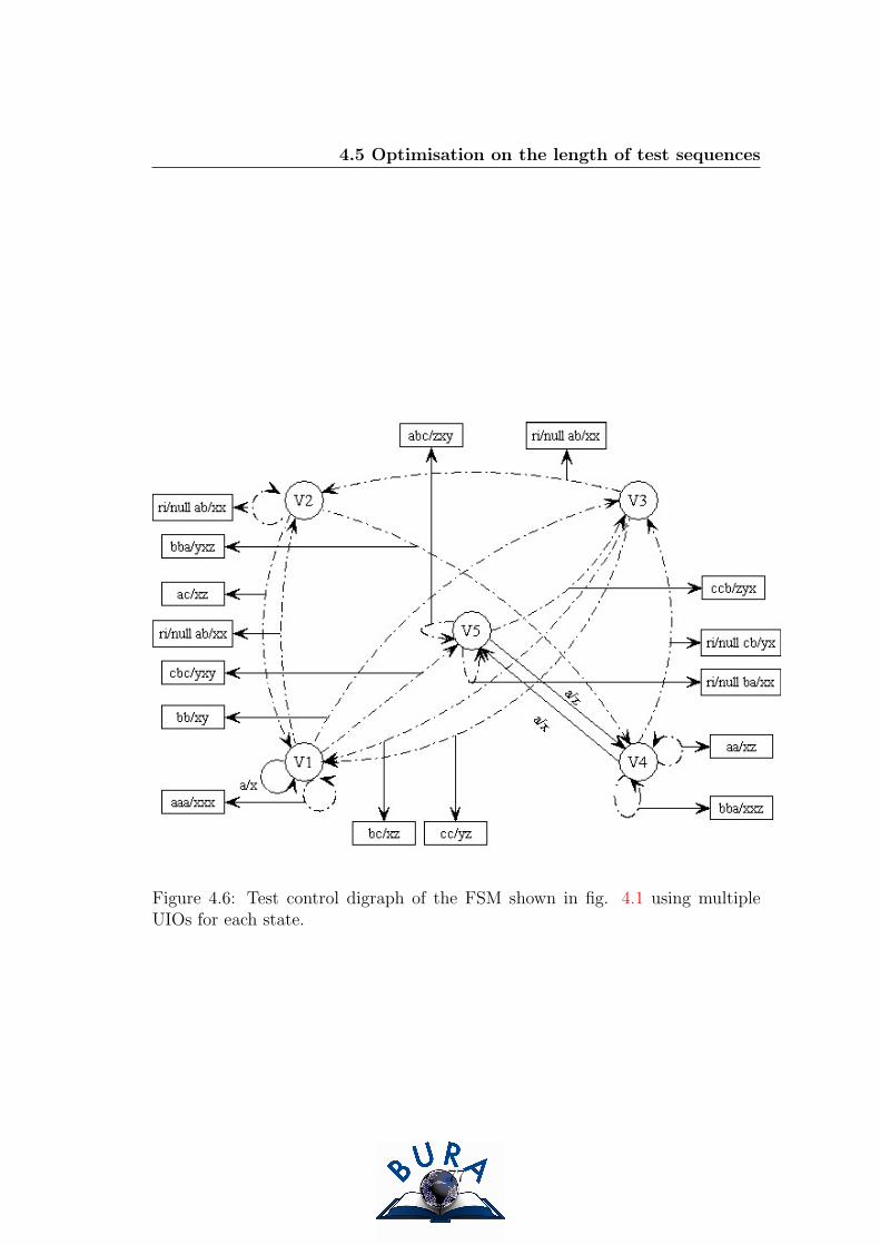
4.5 Optimisation on the length of test sequences
Figure 4.6: Test control digraph of the FSM shown in fig. 4.1 using multipleUIOs for each state.
77

4.5 Optimisation on the length of test sequences
Figure 4.7: Flow network used for the selection of UIOs to generate optimal testcontrol digraph for the FSM shown in fig. 4.1.
78

4.5 Optimisation on the length of test sequences
vertices (states) in the test control digraph D′. If, for all vertices in D
′, there
exist ξ(vi) = 0, i = 1, ..., n, then the test control digraph is symmetric and no
replication is required. The cost of the test sequence is simply the cost of the
edges in EC . In Aho et al.’s method, only one UIO is applied for each state.
The index ξ(vi), i = 1, ..., n, is thus fixed and is usually not equal to zero. This
requires the symmetric augmentation by replicating some edges for a number of
times, which consequently increases the length of the test sequence. It shall be
noted that for a vertex vi, its out-degree d−(vi) in the test control digraph D′is
always the same as that in D, but its in-degree d+(vi) may vary if different UIOs
are selected for a state when generating the test control digraph. Appropriate
selection of a UIO for a transition test will lead to a minimal value of∑n
i=1 |ξ(vi)|in D
′, which determines that the times for replicating edges in D is minimal. The
problem is defined as follows:
Given an FSM M represented by digraph D and a set of UIOs, MUIOj =
{UIO1j , ..., UIO
rj}, for each state sj ∈ S, find an element UIOα
j ∈ MUIOj for
transition (vi, vj; am/on) such that, in the final test control digraphD′,∑n
i=1 |ξ(vi)|is minimal. Selection of a UIO for a transition test can be determined by con-
structing a network DM and then finding a maximum-flow/minimum-cost flow F
on DM . The technique is described as follows:
Given M represented by D, DM is defined as VM = X × Y × {s, t} where
X = {x1, ..., xn}, Y = {y1, ..., yn} and X ≡ Y ≡ V (D)1; s is the source and
t the sink; EM = ES ∪ E+T ∪ E−
T ∪ E∗ where ES = {(s, xi),∀xi ∈ X}, E−T =
{(yj, t),∀yj ∈ Y }, E+T = {(yk, t),∀yk ∈ Y } and E∗ = {(xi, yj;UIOi), ∀ UIOi ∈
MUIOi, Tail(UIOi) = sj}; each edge (s, xi) ∈ ES has zero cost and capacity
u(s, xi)=d+(vi); for each yj ∈ Y , two edges are used to link yj with t, one of which
has a positive cost, while, the other has a negative cost; each edge (yj, t) ∈ E−T
has cost -1 and capacity u(yj, t)=d−(vj); each edge (yj, t) ∈ E+
T has +1 cost and
infinite capacity; each edge (xi, yi) ∈ E∗ has zero cost and infinite capacity. A
flow FM on DM is defined as a function F : EM → Z+ such that:
1. ∀xi ∈ X, F (s, xi) =∑
(xi,yj)∈E∗ F (xi, yj);
2. ∀yj ∈ Y , F (yj, t)+ + F (yj, t)
−=∑
(xi,yj)∈E∗ F (xi, yj);
1X and Y are two complete sets of states denoted with different notations.
79
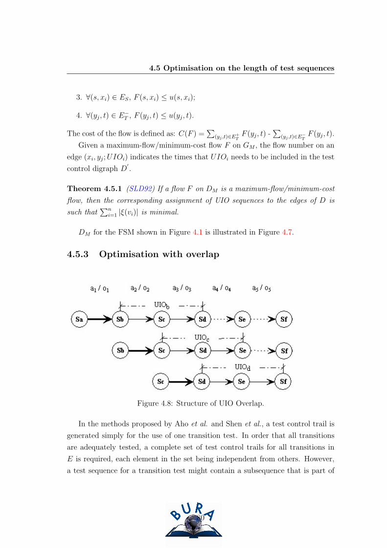
4.5 Optimisation on the length of test sequences
3. ∀(s, xi) ∈ ES, F (s, xi) ≤ u(s, xi);
4. ∀(yj, t) ∈ E−T , F (yj, t) ≤ u(yj, t).
The cost of the flow is defined as: C(F ) =∑
(yj ,t)∈E+TF (yj, t) -
∑(yj ,t)∈E−
TF (yj, t).
Given a maximum-flow/minimum-cost flow F on GM , the flow number on an
edge (xi, yj;UIOi) indicates the times that UIOi needs to be included in the test
control digraph D′.
Theorem 4.5.1 (SLD92) If a flow F on DM is a maximum-flow/minimum-cost
flow, then the corresponding assignment of UIO sequences to the edges of D is
such that∑n
i=1 |ξ(vi)| is minimal.
DM for the FSM shown in Figure 4.1 is illustrated in Figure 4.7.
4.5.3 Optimisation with overlap
Figure 4.8: Structure of UIO Overlap.
In the methods proposed by Aho et al. and Shen et al., a test control trail is
generated simply for the use of one transition test. In order that all transitions
are adequately tested, a complete set of test control trails for all transitions in
E is required, each element in the set being independent from others. However,
a test sequence for a transition test might contain a subsequence that is part of
80
4.5 Optimisation on the length of test sequences
a test sequence for another transition test. The structure of two test sequences
overlap.
Figure 4.8 illustrates an example. In the figure, a transition (sa, sb; a1/o1) is
tested by test sequence TS1 = (a1/o1) · (a2/o2) · (a3/o3). It can be noted that se-
quence (a2/o2)·(a3/o3) is also a part of test sequence TS2, TS2 = (a2/o2)·(a3/o3)·(a4/o4), that tests transition (sb, sc; a2/o2). Sequence (a2/o2) · (a3/o3) is the over-
lapped segment between TS1 and TS2. Test sequence TS3 = (a1/o1) · (a2/o2) ·(a3/o3) contains overlapped segments with TS1, (a3/o3), and TS2, (a3/o3)·(a4/o4)·(a5/o5) as well; if being applied to the FSM, test sequence (a1/o1)·(a2/o2)·(a3/o3)·(a4/o4)·(a5/o5) will test transitions (sa, sb; a1/o1) (sb, sc; a2/o2) and (sb, sc; a3/o3)
successively.
Clearly, a test sequence generated by considering overlap among test sequences
for a set of ordered and distinct transitions is shorter than that generated by
concatenating test sequences that individually test each transition in the set. If,
in a test sequence for the FSM under test, the overall overlap among test sequences
for all transitions in E is maximised, the test sequence is of the minimal length.
This leads to the problem of finding a set of ordered transitions such that overlap
formed among the corresponding test sequences are maximised.
Yang et al. (YU90) and Miller (MP93) show that overlap can be used in con-
junction with multiple UIOs to further reduce the test sequence length. Hierons
(Hie96; Hie97) represents overlap by invertible sequence. All of their work aims
to generate a set of fully overlapped transition sequences, each of which is used
to generate a test control trail in the test control digraph. The test sequence
derived from such a test control digraph is of the minimal length.
Definition 4.5.1 A fully overlapped transition sequence (FOTS) is a sequence of
distinct transitions such that if it is followed by a state identification sequence for
the end state of the last transition in the sequence (so this transition is verified),
then all other transitions in the sequence are also verified.
Definition 4.5.2 A transition (si, sj; am/on) ∈ E is an invertible transition if
and only if it is the only transition entering state sj that involves input am and
output on.
81

4.6 Other finite state models
Definition 4.5.3 A sequence of transitions t = t1...tn, with ti = (si, sj; ami/oni
),
ami∈ I, oni
∈ O, is an Invertible Sequence (IS) if si is the only state that produces
output sequence on1 ...onn and moves to state sj when input am1 ...amn is applied.
4.6 Other finite state models
Except for ordinary finite state machines, some other finite state models have
been proposed for system modelling and testing, including Extended Finite State
Machines (EFSMs), Communicating Finite State Machines (CFSMs) and Prob-
abilistic Finite State Machines (PFSMs).
Definition 4.6.1 An extended finite state machine (EFSM) EM is a quintuple
EM = (I, O, S,−→x , T )
where I, O, S, −→x and T are finite sets of input symbols, output symbols, states,
variables, and transitions, respectively. Each transition t in the set T is a six-tuple
t = (st, qt, at, Pt, At)
where st, qt and at are the start (current) state, end (next) state, input, and
output, respectively. Pt(−→x ) is a predicate on the current variable values and
At(−→x ) gives an action on variable values.
Definition 4.6.2 A communicating finite state machine (CFSM) CM is a 7-
tuple
CM = (I, O, Si, Ai, δi,Mi, s0i)
where I and O are the input set and output set respectively. Si is the set of local
states of machine Mi, s0i∈ Si is the initial state of machine Mi; Ai = ∪1≤j≤nAi,j⋃
∪1≤j≤nAj,i where Ai,j, 1 ≤ j ≤ n is the alphabet of messages that Mi can send
to Mj, and Aj,i, 1 ≤ j ≤ n is the alphabet of messages that Mi can receive from
Mj. δi : Si × Ai × I → Si is the transition function. δi(p,−m, j) is the set of
states that process Mi could move to from state p after sending a message m to
process Mj. δi(p,+m, j) is the set of states that process Mi could move to from
state p after receiving a message m sent by process Mj.
82

4.6 Other finite state models
Obviously, a CFSM is equivalent to an EFSM. One can simply add a variable
to encode the component machines and represent the CFSM by an EFSM. An
EFSM with finite variable domains is a compact representation of an FSM (LY96).
Therefore, the process of testing an EFSMs can be reduced to that of testing
an ordinary FSMs by expanding the EFSM into an equivalent FSM. Once the
conversion is complete, an optimal test sequence can be generated using the
methods discussed above.
Definition 4.6.3 A probabilistic finite state machine (PFSM) PM is a quintuple
PM = (I, O, S, T, P )
where I, O, S, T are the input set, output set, state set, and transition set,
respectively. Each transition t ∈ T is a tuple t = (si, sj, a, o) consisting of the start
(current) state si ∈ S, next state sj ∈ S, input symbol a ∈ I and output symbol
o ∈ O. P is a function that assigns a number P (t) ∈ [0, 1] to each transition t (its
probability), so that for every state s and input symbol a,∑
sj ,o P (s, sj, a, o) = 1.
A PFSM can be represented by a transition graph with n nodes corresponding
to the n states and directed edges between states corresponding to the transition
with nonzero probability. Specifically, if P (si, sj; a/o) > 0, then there is an edge
from si to sj with an associated input a and output o; otherwise, there is no
corresponding edge.
Conformance testing for PFSM is to check whether an implementation PFSM
confirms to a specification PFSM where the term of “conformance” can be defined
in different ways (LY96). Conformance test for PFSM has not been extensively
studied and the study of PFSM remains an open research topic (LY96).
83

Chapter 5
Construction of UIOs
5.1 Introduction
Unique Input/Output (UIO) sequences are often applied for state verification in
finite state machine based testing. A UIO sequence for state si in a finite state
machine M is an input/output sequence x/y, that may be observed from si, such
that the output sequence produced by the machine in response to x from any
other state is different from y. A prerequisite for UIO-based techniques is that
there exists at least one UIO sequence for each state in the finite state machine
under test. Thus, finding ways to (effectively) construct UIOs from a finite state
machine is very important.
Unfortunately, computing UIOs is NP-hard (LY94). Lee and Yannakakis
(LY94) note that adaptive distinguishing sequences and UIOs may be produced
by constructing a state splitting tree1. However, no rule is explicitly defined to
guide the construction of an input sequence. Naik (Nai97) proposes an approach
to construct UIOs by introducing a set of inference rules. Some minimal length
UIOs are found. These are used to deduce some other states’ UIOs. A state’s
UIO is produced by concatenating a sequence to another state, whose UIO has
been found, with this state’s UIO sequence. Although it may reduce the time
taken to find some UIOs, the inference rule inevitably increases a UIO’s length,
which consequently leads to longer test sequences.
1For more about state splitting tree, see chapter 4.
84

5.2 Constructing UIOs with MOTs
Metaheuristic Optimisation Techniques (MOTs) such as Genetic Algorithms
(GAs) (Gol89) and Simulated Annealing (SA) (KGJV83; MRR+53) have proven
efficient in search and optimisation and have shown their effectiveness in provid-
ing good solutions to some NP–hard problems such as the Travelling Salesman
Problem (CCPS98). When searching for optimal solutions in multi-modal func-
tions, the use of sharing techniques is likely to lead to a population that contains
several sub-populations that cover local optima (GR87). This result is useful
since in some search problems we wish to locate not only global optima, but also
local optima.
In this chapter, a model is proposed for the construction of UIOs by using
MOTs. A fitness function is defined to guide the search of input sequences that
constitute UIOs for some states. The fitness function works by encouraging the
early occurrence of discrete partitions in the state splitting tree constructed by
an input sequence while punishing the length of this input sequence.
The study of the proposed model consists of two stages. In the first stage, the
performance of GA on the construction of UIOs was initially investigated. Two
simple FSMs were used for the experiments. The experiments were designed
only to compare the performance between GAs and random search; in the sec-
ond stage, a more thorough study was carried on where sharing techniques are
applied. The use of a sharing technique forces the population of the genetic pool
to form sub-populations, each of which aims to explore UIOs that are calculated
as local optima. This helps to maintain the diversity of the genetic pool. A set of
experiments is designed to study the performance of GAs, GAs with sharing, SA
and SA with sharing respectively. The related work is discussed in the following
sections.
5.2 Constructing UIOs with MOTs
5.2.1 Solution representation
When applying MOTs to a finite state machine, the first question that has to be
considered is what representation is suitable. In this work, the potential solutions
in a genetic pool are defined as strings of characters from the input set I. A DO
85

5.2 Constructing UIOs with MOTs
NOT CARE character ′]′ is also used to further maintain diversity (this is
explained in section 5.4). When receiving this input, the state of a finite state
machine remains unchanged and no output is produced. When a solution is
about to be perturbed to generate a new one in its neighbourhood, some of the
characters in this solution are replaced with characters randomly selected from
the rest of the input set, including ′]′.
5.2.2 Fitness definition
A key issue is to define a fitness function to (efficiently) evaluate the quality of
solutions. This function should embody two aspects: (1) solutions should create
as many discrete units as possible; (2) the solution should be as short as possible.
The function needs to make a trade–off between these two points.
This work uses a function that rewards the early occurrence of discrete parti-
tions and punishes the chromosome’s length. An alternative would be to model
the number of state partitions and the length of a solution as two objectives
and then treat them as multi–objective optimisation problems (for more infor-
mation on multi–objective optimisation problems with GA see, for example, ref.
(Gol89)).
A fitness function is defined to evaluate the quality of an input sequence.
While applying an input sequence to a finite state machine, at each stage of a
single input, the state splitting tree constructed is evaluated by equation 5.1,
f(i) =xie
(δxi)
lγi+ α
(yi + δyi)
li. (5.1)
where i refers to the ith input character. xi denotes the number of existing discrete
partitions while δxi is the number of new discrete partitions caused by the ith
input. yi is the number of existing separated groups while δyi is the number of
new groups. li is the length of the input sequence up to the ith element (Do Not
Care characters are excluded). α and γ are constants. It can be noted that a
partition that finds a new discrete unit creates new separated groups as well.
Equation 5.1 consists of two parts: exponential part, fe(i) = xie(δxi)
lγi, and
linear part, fl(i) = α (yi+δyi)li
. It can be seen that the occurrence of discrete parti-
tions makes xi and δxi increase. Consequently, xie(δxi) is increased exponentially.
86

5.2 Constructing UIOs with MOTs
Figure 5.1: Two patterns of partitions.
Meanwhile, with the input sequence’s length li increasing, lγi is increased expo-
nentially (γ should be greater than 1). Suppose xi and li change approximately
at the same rate, that is δxi ≈ δli, as long as e(δxi) has faster dynamics than lγi ,
fe(i) increases exponentially, causing fi to be increased exponentially. However,
if, with the length of the input sequence increasing, no discrete partition is found,
fe(i) decreases exponentially, causing fi to be decreased exponentially. fe(i) thus
performs two actions: encouraging the early occurrence of discrete partitions and
punishing the increment of an input sequence’s length.
fl(i) also affects f(i) in a linear way. Compared to fe(i), it plays a less impor-
tant role. This term rewards partitioning even when discrete classes have not
been produced. Figure 5.1 shows two patterns with no discrete partition. We
believe pattern B is better than A since B might find more discrete units in the
forthcoming partitions.
Individuals that find discrete partitions at the first several inputs but fail
to find more in the following steps may obtain higher fitness values than others.
They are likely to dominate the population and cause the genetic pool to converge
prematurely. To balance the evaluation, after all input characters have been
examined, the final fitness value for an input candidate is defined as the average
of equation 5.1
F =1
N
N∑i=1
f(i). (5.2)
87
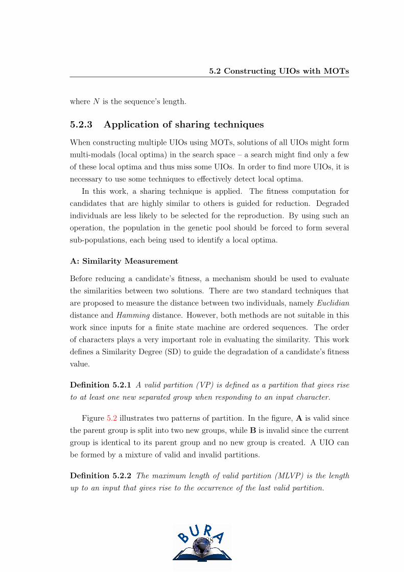
5.2 Constructing UIOs with MOTs
where N is the sequence’s length.
5.2.3 Application of sharing techniques
When constructing multiple UIOs using MOTs, solutions of all UIOs might form
multi-modals (local optima) in the search space – a search might find only a few
of these local optima and thus miss some UIOs. In order to find more UIOs, it is
necessary to use some techniques to effectively detect local optima.
In this work, a sharing technique is applied. The fitness computation for
candidates that are highly similar to others is guided for reduction. Degraded
individuals are less likely to be selected for the reproduction. By using such an
operation, the population in the genetic pool should be forced to form several
sub-populations, each being used to identify a local optima.
A: Similarity Measurement
Before reducing a candidate’s fitness, a mechanism should be used to evaluate
the similarities between two solutions. There are two standard techniques that
are proposed to measure the distance between two individuals, namely Euclidian
distance and Hamming distance. However, both methods are not suitable in this
work since inputs for a finite state machine are ordered sequences. The order
of characters plays a very important role in evaluating the similarity. This work
defines a Similarity Degree (SD) to guide the degradation of a candidate’s fitness
value.
Definition 5.2.1 A valid partition (VP) is defined as a partition that gives rise
to at least one new separated group when responding to an input character.
Figure 5.2 illustrates two patterns of partition. In the figure, A is valid since
the parent group is split into two new groups, while B is invalid since the current
group is identical to its parent group and no new group is created. A UIO can
be formed by a mixture of valid and invalid partitions.
Definition 5.2.2 The maximum length of valid partition (MLVP) is the length
up to an input that gives rise to the occurrence of the last valid partition.
88

5.2 Constructing UIOs with MOTs
Figure 5.2: Patterns of valid partition (A) and invalid partition (B).
Definition 5.2.3 The maximum discrete length (MDL) is the length up to an
input character that gives rise to the occurrence of the last discrete partition.
Since a discrete partition defines a valid partition, MDL can never be greater
than MLVP in a state splitting tree.
Definition 5.2.4 The Similarity Degree (SD) between two ordered sequences is
defined as the length of a maximum length prefix sequence of these two sequences.
If elements in two ordered sequences are the same before the N th character
and different at the N th, the SD is N − 1 (] is excluded from the calculation).
For example, the SD between a#b#aaca##a and ab#a#bc#a#a is 3.
B: Fitness Degrade
In order to prevent the population from converging at one or several global optima
in the search space, at each iteration of computation, some candidates (that are
not marked as degraded) that have high SD value should have the fitness value
reduced by the mechanism as follows:
1. if a candidate’s SD is greater than or equal to its MDL, its fitness value
should be degraded to a very small value; else
89
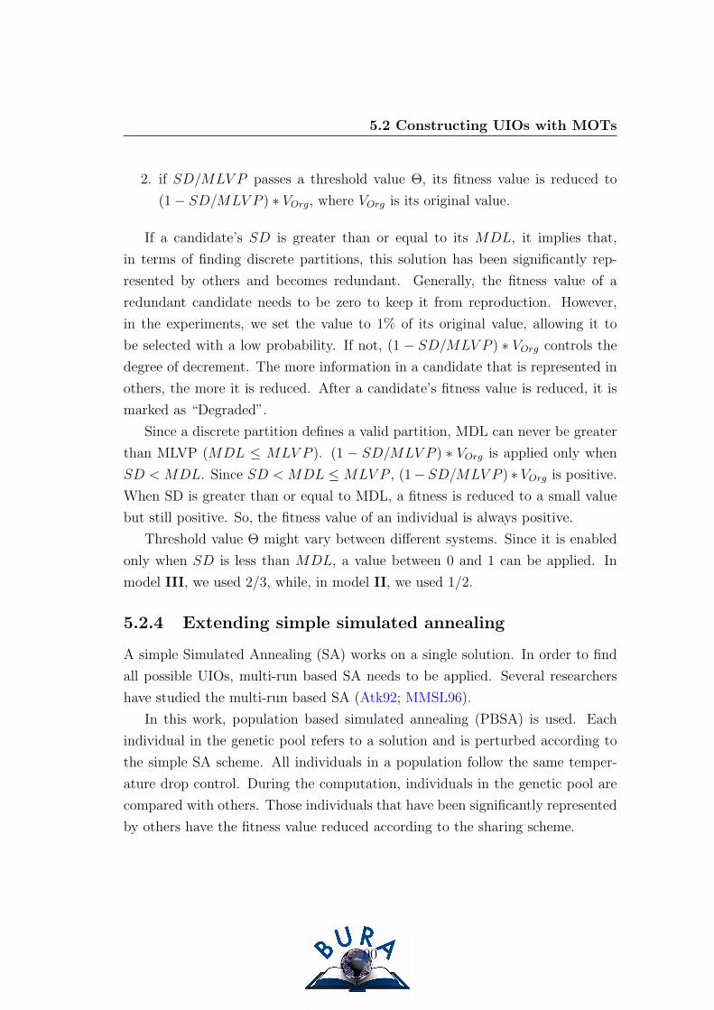
5.2 Constructing UIOs with MOTs
2. if SD/MLV P passes a threshold value Θ, its fitness value is reduced to
(1− SD/MLV P ) ∗ VOrg, where VOrg is its original value.
If a candidate’s SD is greater than or equal to its MDL, it implies that,
in terms of finding discrete partitions, this solution has been significantly rep-
resented by others and becomes redundant. Generally, the fitness value of a
redundant candidate needs to be zero to keep it from reproduction. However,
in the experiments, we set the value to 1% of its original value, allowing it to
be selected with a low probability. If not, (1 − SD/MLV P ) ∗ VOrg controls the
degree of decrement. The more information in a candidate that is represented in
others, the more it is reduced. After a candidate’s fitness value is reduced, it is
marked as “Degraded”.
Since a discrete partition defines a valid partition, MDL can never be greater
than MLVP (MDL ≤ MLV P ). (1 − SD/MLV P ) ∗ VOrg is applied only when
SD < MDL. Since SD < MDL ≤MLV P , (1− SD/MLV P ) ∗ VOrg is positive.
When SD is greater than or equal to MDL, a fitness is reduced to a small value
but still positive. So, the fitness value of an individual is always positive.
Threshold value Θ might vary between different systems. Since it is enabled
only when SD is less than MDL, a value between 0 and 1 can be applied. In
model III, we used 2/3, while, in model II, we used 1/2.
5.2.4 Extending simple simulated annealing
A simple Simulated Annealing (SA) works on a single solution. In order to find
all possible UIOs, multi-run based SA needs to be applied. Several researchers
have studied the multi-run based SA (Atk92; MMSL96).
In this work, population based simulated annealing (PBSA) is used. Each
individual in the genetic pool refers to a solution and is perturbed according to
the simple SA scheme. All individuals in a population follow the same temper-
ature drop control. During the computation, individuals in the genetic pool are
compared with others. Those individuals that have been significantly represented
by others have the fitness value reduced according to the sharing scheme.
90

5.3 Models for experiments
Figure 5.3: The first finite state machine used for experiments: model I.
5.3 Models for experiments
The study of the proposed model consists of two stages. In the first stage, the
construction of UIOs using GAs was initially investigated. The performance of
GAs was simply compared with that of random search. In the second stage,
we investigated the impact of the sharing technique when constructing multiple
UIOs using GAs and SA, and reported the experimental results.
Three models are used for experiments. These models are minimal and
strongly connected. They are shown in Figure 5.3 (model I), Figure 5.4 (model
II) and Figure 5.5 (model III), respectively.
The first model has 5 states. The input set is I = {a, b, c} and the output set
is O = {x, y}; the second model has 10 states and the third model has 9 states.
Both the second and the third machines use the same input and output sets. They
are: I = {a, b, c, d} and O = {x, y, z}. The complete set of the minimum-length
UIOs for model I is listed in Table 5.1.
When investigating the impact of the sharing techniques, in order to compare
91
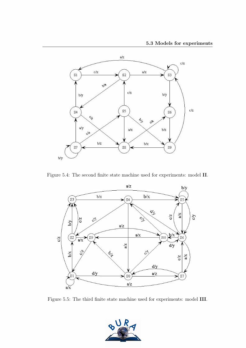
5.3 Models for experiments
Figure 5.4: The second finite state machine used for experiments: model II.
Figure 5.5: The third finite state machine used for experiments: model III.
92

5.4 Working with genetic algorithms
State UIOsaa/xx, ab/xx, ac/xy, ba/xx
s1 bb/xy, ca/yx, cb/yxs2 b/ys3 ba/xz, bc/xz, ca/yz, cc/yzs4 bb/xx, bc/xys5 a/z, c/z
Table 5.1: The minimum-length UIOs for model I.
SQ NS SQ NS SQ NS SQ NScbb 7 cbca 6 bca 5 cacc 4bcb 7 bcc 6 ccb 4 caca 4bb 7 cacb 5 cbc 4 caa 4
cbcc 6 vab 5 cba 4 acb 4ab 4 ca 3 aa 3 a 2ccc 3 bcbc 3 cc 2 bc 1cca 3 acc 3 bcba 2 - -cb 3 aca 3 ba 2 - -
Table 5.2: UIOs for model II.
the set of UIOs produced with a known complete set, the search is restricted to
UIOs of length 4 or less. With such a restriction, for model II and model III,
44 = 256 input sequences can be constructed. There are 30 UIOs for model II,
listed in Table 5.2 and 86 UIOs for model III, listed in Table 5.3. In the tables,
SQ stands for the input from a UIO sequence and NS refers to the number of
states this sequence can identify.
5.4 Working with genetic algorithms
5.4.1 GA vs. random search
In this section, a set of experiments was devised to investigate the performance
of a simple GA on the construction of UIOs. The experiments were designed by
using model I first, and then model II. The performance of a simple GA was
experimentally compared with that of random search.
93

5.4 Working with genetic algorithms
SQ NS SQ NS SQ NS SQ NSaaaa 8 aaa 5 bcca 5 accd 4aaab 7 aabc 5 bccb 5 bab 4cca 7 aacc 5 cbcd 5 baca 4ccb 7 abca 5 ccc 5 bacb 4aaad 6 acaa 5 aabb 4 bbc 4aaca 6 acad 5 aabd 4 bca 4acca 6 baa 5 abcc 4 bcba 4accb 6 bba 5 abcd 4 bcbc 4accc 6 bbb 5 aca 4 bcbd 4cbca 6 bcad 5 acba 4 bccc 4cbcc 6 bcbb 5 acbb 4 caaa 4caab 4 bcc 3 aadc 2 ca 1cbaa 4 bcd 3 abd 2 aad 1cbaa 4 bcd 3 abd 2 aad 1cbb 4 caac 3 acbd 2 acb 1cbcb 4 cabc 3 ba 2 ada 1aab 3 cacc 3 caa 2 adba 1aba 3 cbab 3 cabb 2 adbc 1abb 3 cbd 3 cabd 2 adbd 1abc 3 aacb 2 caca 2 adc 1bacc 3 ccb 2 cacb 2 cd 1bad 3 aacd 2 cad 2 bb 3aada 2 cb 2 - - - -
Table 5.3: UIOs for model III.
94
5.4 Working with genetic algorithms
A: Tracking historical records
When implementing GAs, mutation prevents the computation from getting stuck
in a local maxima/minima but might also force it to jump out of the global
maxima/minima when it happens to be there. Solutions provided at the end of
evolutionary computation could be good, but need not be the best found during
the process. It is therefore useful to keep track of those candidates that have
produced good or partially good solutions, and store them for the purpose to
further optimise the final solutions.
Consider an example shown in Figure 5.6. Suppose that a GA produces a
UIO sequence Ut for state st, forming a path shown in thin solid arrow lines.
During the computation, another solution U ′t for st has been found, forming a
path shown in dotted arrows. The two lines visit a common node at N4. Ut has
a shorter path than U ′t before N4 while has a longer path after N4. The solution
recombined from Ut and U ′t (indicated in figure by thick arrow lines), taking their
shorter parts, is better than either of them.
In the study of computing UIOs using a simple GA, a database is used to track
candidates that result in the occurrence of discrete partitions. This database is
then used to further optimise the final solutions through recombination. Solutions
for a state, which are of the same length, are multi-UIOs for this state which can
be used in test generation proposed in refs. (SLD92; YU90).
B: Experiments with model I
Goldberg (Gol89) has studied the effects of different choices of crossover and
mutation rates. In this work, we simply follow his suggestions. The parameters
are set to: 1ChrLen = 10, XRate = 0.75, MRate = 0.05, PSize = 30, MGen =
50, α = 15, and γ = 1.5. The settings of crossover rate and mutation rate remain
unchanged throughout all GA experiments.
Model I is first used for the experiments. All minimum-length UIOs for all
states are presented in Table 5.1. Roulette Wheel Selection (RWS) and Uniform
Crossover (UC) are implemented.
1ChrLen:Chromosome Length; XRate:Crossover Rate; MRate:Mutate Rate; PSize: Popu-lation Size; MGen:The Maximum Number of Generations.
95

5.4 Working with genetic algorithms
Figure 5.6: Solution recombination.
96
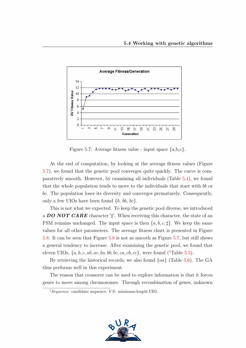
5.4 Working with genetic algorithms
Figure 5.7: Average fitness value - input space {a,b,c}.
At the end of computation, by looking at the average fitness values (Figure
5.7), we found that the genetic pool converges quite quickly. The curve is com-
paratively smooth. However, by examining all individuals (Table 5.4), we found
that the whole population tends to move to the individuals that start with bb or
bc. The population loses its diversity and converges prematurely. Consequently,
only a few UIOs have been found {b, bb, bc}.This is not what we expected. To keep the genetic pool diverse, we introduced
a DO NOT CARE character ′]′. When receiving this character, the state of an
FSM remains unchanged. The input space is then {a, b, c, ]}. We keep the same
values for all other parameters. The average fitness chart is presented in Figure
5.8. It can be seen that Figure 5.8 is not as smooth as Figure 5.7, but still shows
a general tendency to increase. After examining the genetic pool, we found that
eleven UIOs, {a, b, c, ab, ac, ba, bb, bc, ca, cb, cc}, were found (1Table 5.5).
By retrieving the historical records, we also found {aa} (Table 5.6). The GA
thus performs well in this experiment.
The reason that crossover can be used to explore information is that it forces
genes to move among chromosomes. Through recombination of genes, unknown
1Sequence: candidate sequence. V S: minimum-length UIO.
97

5.4 Working with genetic algorithms
ID Sequence ID Sequence1 bccaabcacc 16 bbcaabcacc2 bbbaabaacc 17 bbbaabaaca3 bbbaabcacc 18 bbcaababcc4 bcccabaacb 19 bbbcabbacc5 bbcbabcacb 20 bbcaabaacc6 bbbaabcacc 21 bccaabaacc7 bbcbabcacb 22 bbbaabaacc8 bbccabcacb 23 bbbcabbacc9 bbcbabaacb 24 bbcbabcacb10 bcbbabaacb 25 bbbcabcacc11 bbcbabcabb 26 bbcaabcacb12 bbcaabaacc 27 bbbbababcc13 bccaabaacb 28 bbcaabcacb14 bbbbabcacc 29 bbccabbacc15 bbcbabcacb 30 bbbaabbacb
Table 5.4: Final sequences obtained from model I - input space {a,b,c}.
Figure 5.8: Average fitness value - input space {a,b,c,]}.
98

5.4 Working with genetic algorithms
ID Sequence VS ID Sequence VS1 bbbbcccb]c bb 16 ]bcbabcabb bc2 ab]bbc]bbc ab 17 ]]cba]cbcb cb3 ]bc]caaaba bc 18 ]bb]]bbaca bb4 ]]bcacbc]c bc 19 bc]bb]cbb] bc5 b]bcaca]cb bb 20 cbcbbc]]ca cb6 bb]bca]]bb bb 21 ]bc]aabc]c bc7 cbacc]ac]b cb 22 c]a]cacc]c ca8 acabaaaacc ac 23 c]accac]]a ca9 ba]a]aaa]b ba 24 ]b]bcabbc] bb10 ]ccaab]acc cc 25 bb]bba]]a] bb11 ]cbc]aa]ab cb 26 bacb]c]b]b ba12 ]bbcca]aaa bb 27 bb]bb]]]c] bb13 cccb]]]]]c cc 28 cb]babc]b] cb14 aca]bbaa]b ac 29 cccc]cc]bb cc15 cbb]c]cb]c cb 30 b]cca]]b]c bc
Table 5.5: Final sequences obtained from model I - input space {a,b,c,]}.
ID Sequence VS Fitness1 aa]caab]c aa 6.27842 a]aba]bc]c aa 4.2605
Table 5.6: Solutions obtained from the historical record database.
99

5.4 Working with genetic algorithms
Exp. UIOs Found Total Percent(%)1 8 12 66.72 8 12 66.73 11 12 91.74 11 12 91.75 10 12 83.36 11 12 91.77 11 12 91.78 11 12 91.79 10 12 83.310 12 12 10011 11 12 91.7
Avg 10.36 12 86.4
Table 5.7: Average result from 11 experiments.
information can be uncovered by new chromosomes. However, the gene move-
ment exerted by crossover can only happen among different chromosomes. We
call it vertical movement. By using a DO NOT CARE character, some spaces
can be added in a chromosome, which makes it possible for genes to move hori-
zontally. Therefore, DO NOT CARE makes the exploration more flexible, and,
consequently, can help to keep the genetic pool diverse.
We organised eleven experiments with the same parameters. By examining
the solutions obtained in the final genetic pool (historical records are excluded),
we evaluated the average performance. Table 5.7 shows that, in the worst case,
8 out of 12 UIOs are found, which accounts for 66.7%. The best case is 100%.
The average is 86.4%.
After examining the solutions from different experiments, we found that aa is
the hardest UIO to be found while bb and bc are most frequent ones that occur
in the final solutions. By checking Table 5.1, we found a very interesting fact: a
majority of UIOs initially start with b or c. If individuals happen to be initialised
with ba××××××××, they will distinguish s1, s2 and s5 in the first two steps,
and so achieve high fitness. These individuals are likely to be selected for the
next generation. Individuals initialised with aa×××××××× can distinguish
only s1 and s5 in the first two steps, and achieve lower fitness values. They are
100

5.4 Working with genetic algorithms
ID Sequence VS ID Sequence VS1 cabbbcbcac ca 16 cacacacccc ca2 ccbcbbbcbc cc 17 bcbbabcbca bc3 bcccaaabcb bc 18 ccccbbcccb cc4 cccccbcbac cc 19 accbbccacb ac5 ccbbacbccc cc 20 cbccaccccb cb6 bccccabcac bc 21 acbbcbbbbb ac7 bccbcbbcbc bc 22 cbccccbccb cb8 ccbbccaabc cc 23 ccabacbcca cc9 bbacccccba bb 24 accacbabcc ac10 cbbbbacccb cb 25 aabcbacbbb aa11 bcaacccccb bc 26 cabbacacbc ca12 cccbcbbcbc cc 27 bcbccccaac bc13 abcbbcccab ab 28 aabcbccbca aa14 bcccccbccc bc 29 bccccaabbb bc15 bbccbccbba bb 30 acaccbaaba ac
Table 5.8: Solutions obtained using by random search.
less likely to be selected for reproduction. This fact seems to imply that there
exist multiple modals in the search space. Most individuals are likely to crowd
on the highest peak. Only a very few individuals switch to the lower modals. To
overcome this problem, sharing techniques might help. The application of such
approaches is studied in the following subsections.
We then turn to compare the performance between GA and random search.
Random search is defined as randomly perturbing one bit in an input sequence.
30 input sequences of ten input characters were randomly generated. We repeated
this experiment 10 times. The results shown in Table 5.8 are the best ones. From
the table it can be seen that 11 out of 12 UIOs (a, b, c, aa, ab, ac, bb, bc, ca, cb,
cc) are found over these experiments. Only one is missed (ba).
B: Experiments with model II
Since model I is comparatively simple, and the UIOs are short, it is not difficult
to find all UIOs through random search. Thus, the GA does not show signifi-
cant advantages over random search. A more complicated system, model II, is
therefore used to further test GA’s performance.
101

5.4 Working with genetic algorithms
State UIOss1 ca/xx, cb/xxs2 aa/xz, ab/xy, acc/xxx, bb/xy
bcc/xxx, bcba/xxzys3 a/z, bb/yz, ca/xz, cb/xy,
ccb/xxy, ccc/xxxs4 bc/yx, cba/xzy, ccb/xxz
cbca/xzzx, cbcc/xzzzs5 ab/xz, acb/xxz, bb/yx
bcc/yzx, cacc/zxxx, cb/zxs6 bb/zx, bcc/zzxs7 a/y, bb/yy, bcc/yzz,
bcbc/yzyz, cbc/zyz, cc/zzs8 bb/zy, bcc/zzz, bcbc/zzyz,
cbca/xzzz, cbcc/xzzxs9 bb/xz, ca/zz, cc/zx
Table 5.9: UIO sequences for model II found by random search.
However, no existing UIOs are available for model II, which means that we
can never be sure that a complete set of UIOs has been found. Hence, we will
compare the numbers of UIOs found by using random search and GA separately.
A total of 50 candidates were used in the experiment. All UIOs found, whether
minimum-length or not, are listed to make a comparison. Experiments on both
random search and GA were repeated 10 times. The solutions presented in Table
5.9 and Table 5.10 are the best. Table 5.9 lists the UIOs obtained through random
search while Table 5.10 shows the solutions found by GA. After comparing these
two tables, we found that GA finds many more UIOs than random search does.
Both random search and GA easily find the short UIOs. However, for other UIOs
the performance of GA appears to be much better than that of random search.
For example, GA finds bcbcc/xxzzz and cbcbb/xzzyz while random search does
not.
We also measured the frequency of hitting UIOs. Random search is redefined
by initialising population routinely. Experimental result show that both methods
hit UIOs with the length of 3 or less frequently. However, on hitting those with
the length of 4, random search is roughly the half times of GA, while, for those
102

5.4 Working with genetic algorithms
State UIOss1 ca/xx, cb/xxs2 aa/xz, ab/xy, aca/xxz,acb/xxy
acc/xxx, bb/xy, bcc/xxx, bcbcc/xxzzzs3 a/z, bb/yz, ca/xz, cb/xy,
ccb/xxy, ccc/xxxbc/yx, cba/xzy,cbcbb/xzzyx
s4 cbb/xzy, ccb/xxz, cbca/xzzx,cbcc/xzzz, cbcbc/xzzyz
s5 ab/xz, acb/xxz, bb/yx, bca/yzzbcc/yzx, cab/zxy, cb/zx
s6 bb/zx, bca/zzz, bcc/zzxa/y, ba/yy, bb/yy, bca/yzx
s7 bcc/yzz, cab/zxz, cbb/zyx, cc/zzcbc/zyz, cc/zz, bcbc/yzyz
ba/zy, bb/zy, bca/zzx,s8 bcc/zzz, cbb/xzx, cbca/xzzz,
cbcc/xzzx, cbcbb/xzzyzs9 bb/xz, ca/zz, cbb/zyz, cc/zx
Table 5.10: UIO sequences for model II found by GA.
103

5.4 Working with genetic algorithms
with the length of 5, in the first 30 iterations, random search hits 10 times while
GA 27.
All these results suggest that, in simple systems, it is possible to obtain good
solutions through random search. However, in more complicated systems, espe-
cially in those with large input and state spaces, finding UIOs with random search
is likely to be infeasible. By contrast, GA seems to be more flexible.
C: summary
In this subsection, the performance on computing UIOs using simple GAs was
investigated. It is shown that the fitness function can guide the candidates to
explore potential UIOs by encouraging the early occurrence of discrete partitions
while punishing length.
It is also demonstrated that using a DO NOT CARE character can help to
improve the diversity in GAs. Consequently, more UIOs can be explored. The
simulation results in a small system showed that, in the worst case, 67% of the
minimum-length UIOs have been found while, in the best case, 100%. On the
average, more than 85% minimum-length UIOs were found from the model under
the test. In a more complicated system, GA found many more UIOs than random
search. GA was much better than random search at finding the longer UIOs.
These experiments and figures suggest that GAs can provide good solutions on
computing UIOs.
However, it was also noted that some UIOs were missed with high probability.
This may be caused by their lower probability distribution in the search space.
The problem was further studied in the next subsection.
5.4.2 Sharing vs. no sharing
Experiments in this subsection investigate the impact of the sharing techniques
that aim to overcome the problem discussed in section 5.4.1. Maximum generation
is set to MGen = 300. The population size is set to PSize = 600. The value of
MGen and PSize remain unchanged throughout all following experiments.
104

5.4 Working with genetic algorithms
The experiments used model III first, and then model II. Threshold value θ
is set to 2/3 for model III and 1/2 for model II. α and γ are set to 20 and 1.2
respectively (section 5.7 explains the reason for choosing such values).
The first experiment studied the UIO distribution when using GA without
sharing. The experiment was repeated 10 times. Figure 5.9 shows the UIO
distribution of the best result. It can be seen that a majority of individuals move
to a sub–population that can identify 7 states. The rest scatter among some
other sub–populations that can identify 8, 6, 5, 4, 3, 2, 1 states. Due to such an
uneven distribution, some sequences that define UIOs of 6, 5, 4, 3, 2, 1 states are
likely to be missed. Only 59 are found and so 27 were missed.
An experiment was then designed to investigate the use of the sharing tech-
nique. This experiment was repeated 10 times. The best result is shown in Figure
5.10 (in B–H, sequences of legends indicate input sequences that define UIOs).
It can be seen that, after applying sharing, the population is generally spread
out, forming 9 sub–populations. Each sub–population contains UIO sequences
that identify 0, 1, 2, 3, 4, 5, 6, 7, 8 states correspondingly. Only 4 UIOs were
missed – the performance of the search had improved dramatically. However, the
distributions in sub–populations do not form a good shape. Each sub–population
is dominated by one or several UIOs.
The impact of sharing techniques was further investigated by using model II.
Figure 5.11 shows the best result from the 5 experiments. It can be seen that
the distribution of input sequences is similar to that of GA with sharing in model
III. Generally, the population is spread out, forming several sub–populations.
However, each sub–population is dominated by several individuals. We found
that 2 UIOs were missed.
The experimental results above suggest that, when constructing UIOs using
a GA, without the sharing technique, the population is likely to converge at
several individuals that have high fitness values. The distribution of such a pop-
ulation causes some UIOs to be missed with high probability. This is consistent
with the results of section 5.4.1. After applying the sharing technique, the pop-
ulation is encouraged to spread out and forms several sub–populations. These
sub–populations are intended to cover all optima in the search space. The search
quality was significantly improved and more UIOs were found.
105

5.4 Working with genetic algorithms
Figure 5.9: UIO distribution using GA without sharing for model III; Legendsindicate the number of states that input sequences identify.
106

5.4 Working with genetic algorithms
Figure 5.10: UIO distribution using GA with sharing for model III.
107

5.4 Working with genetic algorithms
Figure 5.11: UIO distribution using GA with sharing for model II.
108
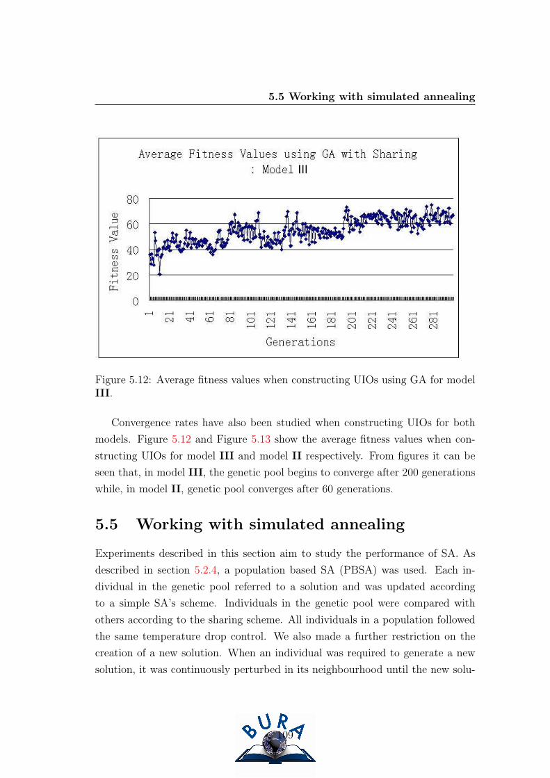
5.5 Working with simulated annealing
Figure 5.12: Average fitness values when constructing UIOs using GA for modelIII.
Convergence rates have also been studied when constructing UIOs for both
models. Figure 5.12 and Figure 5.13 show the average fitness values when con-
structing UIOs for model III and model II respectively. From figures it can be
seen that, in model III, the genetic pool begins to converge after 200 generations
while, in model II, genetic pool converges after 60 generations.
5.5 Working with simulated annealing
Experiments described in this section aim to study the performance of SA. As
described in section 5.2.4, a population based SA (PBSA) was used. Each in-
dividual in the genetic pool referred to a solution and was updated according
to a simple SA’s scheme. Individuals in the genetic pool were compared with
others according to the sharing scheme. All individuals in a population followed
the same temperature drop control. We also made a further restriction on the
creation of a new solution. When an individual was required to generate a new
solution, it was continuously perturbed in its neighbourhood until the new solu-
109

5.5 Working with simulated annealing
Figure 5.13: Average fitness values when constructing UIOs using GA for modelII.
tion found at least one discrete partition. In order to make a comparison with
GA, the maximum number of generations is always set to 300.
Model III was first applied for the experiments. Two temperature drop control
schema were considered. In the first experiment, the temperature was reduced
by a normal exponential function nT (i + 1) = 0.99 ∗ nT (i) (Figure 5.14-A), and
a sharing technique was applied. The experiment was repeated 10 times and the
best result is shown in Figure 5.15.
From the figure it can be seen that the general distribution and sub–population
distributions are quite similar to that of GA with sharing. The population was
formed with several sub–populations. Each sub–population was dominated by
several individuals. A total of 8 UIOs were missed. Compared to the experiments
studied in section 5.4, this figure is quite high. In order to improve the search
quality, the temperature drop scheme was changed to nT (i+ 1) = 0.99 ∗ nT (i) +
nS(i+1)∗sin(10∗π∗i), where nS(i+1) = 0.95∗nS(i). The curve of the function
is shown in Figure 5.14-B. Generally, the tendency of temperature control is
still exponentially decreasing, but local bumps occur. The best result from 10
110

5.5 Working with simulated annealing
Figure 5.14: Simulated annealing temperature drop schema; A: normal exponen-tial temperature drop; B: rough exponential temperature drop.
experiments is shown in Figure 5.16. We find that the distribution of population
and sub–population have no significant changes. However, only 2 UIOs were
missed. The performance is much better than the previous one.
The two SA methods were further studied by using model II. Figure 5.17
shows the best result using the normal temperature drop control while Figure 5.18
shows the best result for the rough temperature drop control. From these figures
it can be seen that, compared to the experiments using model III, the distribution
of input sequences have no significant changes. Both temperature control schemes
achieve a good performance. In normal temperature drop experiment, 3 UIOs
are missed while 2 UIO are missed in rough temperature drop experiment.
Figure 5.19 and Figure 5.20 present the average fitness values when construct-
ing UIOs for model III and model II using rough temperature drop control scheme
respectively. The figures show that, when using model III, the genetic pool be-
gins to converge after 250 generations while, when using model II, the genetic
pool converges after 200 generations. Comparing to Figure 5.12 and Figure 5.13,
it can be seen that SA converges slower than GA.
111

5.5 Working with simulated annealing
Figure 5.15: UIO distribution using SA with normal temperature drop for modelIII.
112

5.5 Working with simulated annealing
Figure 5.16: UIO distribution using SA with rough temperature drop for modelIII.
113

5.5 Working with simulated annealing
Figure 5.17: UIO distribution using SA with exponential temperature drop formodel II.
114
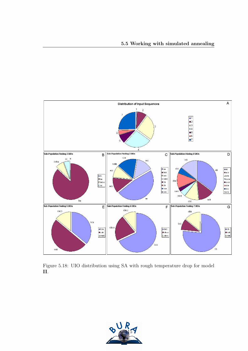
5.5 Working with simulated annealing
Figure 5.18: UIO distribution using SA with rough temperature drop for modelII.
115

5.6 General evaluation
Figure 5.19: Average fitness values when constructing UIOs using SA (rough Tdrop) for model III.
5.6 General evaluation
The experimental results reported in the previous sections suggest that, when
constructing UIOs using GA and SA, without sharing technique, the population
is likely to converge at several individuals that have high fitness values. The
distribution of such a population causes some UIOs to be missed with high prob-
ability. After applying sharing technique, the population is encouraged to spread
out and forms several sub–populations. These sub–populations are intended to
cover all optima in the search space. The search quality significantly improved
and more UIOs were found. Tables 5.11 and 5.12 give the number of UIOs that
are missed for each experiment using GA, SA, GA with sharing and SA with
sharing. From these tables it can be seen that sharing techniques are effective in
finding multiple UIOs. It can also be noted that the performance of the search is
comparatively stable.
It has also been shown that, with the sharing technique, there is no significant
difference between GA and SA on the search for UIOs. Both techniques force their
116

5.6 General evaluation
Figure 5.20: Average fitness values when constructing UIOs using SA (rough Tdrop) for model II.
GA SA GA/S SA/N SA/R1 27 56 4 14 22 29 49 6 18 43 30 62 6 15 44 31 37 7 11 35 29 55 5 9 66 28 48 8 13 57 30 44 7 10 28 27 51 8 13 69 29 39 4 15 410 32 46 7 10 3
Avg 29.2 48.7 6.2 12.8 4.1
Table 5.11: Missing UIOs when using model III; GA:simple GA without sharing;SA:simple SA without sharing; GA/S:GA with sharing; SA/N:SA with sharingusing normal T drop; SA/R:SA with sharing using rough T drop.
117

5.7 Parameter settings
GA SA GA/S SA/N SA/R1 7 15 2 3 22 7 17 4 4 23 9 21 4 3 24 7 19 2 3 35 7 20 3 3 2
Avg 7.2 18.4 3 3.2 2
Table 5.12: Missing UIOs when using model II; GA:simple GA without sharing;SA:simple SA without sharing; GA/S:GA with sharing; SA/N:SA with sharingusing normal T drop; SA/R:SA with sharing using rough T drop.
populations to maintain diversity by forming sub–populations. In the two models
under test, with the sharing technique, both GA and SA are effective.
When applying the SA, rough exponential temperature drop seems to be bet-
ter than the normal exponential temperature drop. Since the sharing technique
reduces some individuals’ fitness values, some information might be lost during
the computation. Local bumping in the rough exponential temperature drop
gives the experiments a second chance for amendments, which might help to pre-
vent such information from being lost. This could explain why the performance
of the rough SA was consistently better than that of a simple SA.
The results on convergence rates imply that, when constructing UIOs, the
GA converges faster than the SA. A simple GA works on population based ex-
ploration. New solutions (children) inherit information from previous solutions
(parents) through crossover while a SA generates a new solution based on the
search in the neighbourhood of an existing solution. A simple GA is more ex-
ploitative than a SA. That might explain why GA converges faster than SA in
our experiments.
5.7 Parameter settings
Parameter settings on crossover and mutation rates follow the suggestions from
ref. (Gol89); When investigating the impact of a sharing technique, the pop-
ulation size used in all experiments is fixed to 600. Using a larger size for a
population may increase the chance on finding more UIOs, but it increases the
118

5.7 Parameter settings
computational cost as well. This work did not investigate the effects on varying
crossover rate, mutation rate and the population size. Future work will address
these issues.
Parameter settings for α and γ affect the performance of computation signif-
icantly. γ is defined to control the dynamic behaviour of the exponential part in
the fitness function while α adjusts the weight of the linear part. To counteract
the effect of xieδxi , γ must be set to a value that is greater than 1. However,
it can also be noted that too big a value of γ causes the calculation of an indi-
vidual’s fitness a continuous decrement even when some discrete partitions are
found. Therefore, a comparative small value that is greater than 1 should be
considered. In this work, we found that setting γ between 1.2 and 1.5 achieves
better performance than other values.
α is defined to reward the partitions when no discrete class has been found.
Normally, at the beginning of computation, when no discrete class is found, the
linear part plays the major role in the calculation of the fitness value. However,
with the computation going further and some discrete classes being found, the
exponential part takes over the role and becomes the major factor. Individuals
that switch the role too slowly might obtain low fitness values and become unlikely
to be selected for reproduction. This effect might cause some patterns (some
UIOs) to be missed.
For example, Figure 5.21 shows two patterns of state splitting trees in model
III. In pattern A (corresponding to aaaa), there are 5 discrete units in the fourth
layer (corresponding to the first three inputs) and 3 units in the fifth layer (cor-
responding to the first four inputs). In pattern B (corresponding to ccac), there
is 1 discrete unit in the third layer (corresponding to the first two inputs) and 6
units in the fourth layer (corresponding to the first three inputs). ccac acquires a
much higher fitness value than that of aaaa. aaaa is therefore likely to be missed
during the computation. To compensate for this effect, a comparatively high α
value might be helpful since it enhances the effect of the linear action. In this
work, we set α to 20. We have also tested values that are below 15 and found
that no experiment discovered the pattern A (aaaa).
Threshold value θ decides whether the fitness value of a candidate can be
reduced. A value between 0 and 1 can be applied. The setting of θ should be
119

5.7 Parameter settings
Figure 5.21: Two patterns of state splitting tree generated from model III.
120

5.8 Summary
suitable and may vary in different systems. If θ is set too low, candidates that
are not fully represented by others may be degraded, causing some UIOs to be
missed. For instance, abcab and abaac are two candidates. If θ is set less than
0.4, compared with abcab, the fitness value of abaac can be degraded. However, it
can be seen that abaac is not fully represented by abcab. abaac might be missed
in the computation due to inappropriate operations; at the same time, too high
a value of θ might make the operation of fitness degrade ineffective. If θ is set to
1, no degrade action occurs.
In our experiments, 2/3 was used in model III while 1/2 was selected for
model II; these values were chosen after some initial experiments.
5.8 Summary
State verification using Unique Input/Output (UIO) sequences has been playing
a very important role in the automated generation of test sequences when testing
from finite state machines. Finding ways to effectively construct UIO sequences
for each state from the finite state machine being investigated is extremely im-
portant. However, computing UIO sequences is NP-hard.
In this chapter, we investigated the use of Metaheuristic Optimisation Tech-
niques (MOTs), with sharing, in the generation of (multiple) unique input output
sequences (UIOs) from a finite state machine (FSM). A fitness function, based
on properties of a state splitting tree, guides the search for UIOs.
The performance of a simple Genetic Algorithm (GA) was experimentally
compared to that of random search by using two finite state machines. The
experimental results suggested that the GA outperforms random search.
A sharing technique was introduced to maintain the diversity in a population
by defining a mechanism that measures the similarity of two sequences. Two
finite state machines were used to evaluate the effectiveness of a GA, GA with
sharing, and a Simulated Annealing (SA) with sharing. The experimental results
showed that, in terms of UIO distributions, there was no significant difference
between the GA with sharing and the SA with sharing. Both outperforms the
version of the GA without sharing. With the sharing technique, both GA and
SA can force a population to form several sub-populations and these are likely
121

5.8 Summary
to cover many local optima. By finding more local optima, the search identifies
more UIOs.
However, a problem is also noted. All sub-populations are dominated by one
or several individuals. This remains a research topic for the future work.
122

Chapter 6
Fault coverage
6.1 Introduction
Testing is an expensive process. Finding effective strategies to automate the
generation of efficient tests, which can help to reduce development costs and to
improve the quality of (or at least confidence in) a system, is of great value in
reducing the cost of system development and testing.
When testing from a finite state machine (FSM) M , an efficient test sequence
should cover, as much as possible, all faults which any implementation may have
and should be relatively short. Ideally we use a complete test suite: a test
suite that is guaranteed to determine correctness if the number of states of the
Implementation Under Test (IUT) does not exceed some predetermined bound.
However, all approaches to generating a complete test suite either rely on the
existence of a distinguishing sequence for M (Gon70; Hen64; UWZ97), assume
that the IUT has a reliable reset (Cho78), or produce a test suite whose size is
exponential in terms of the number of states of M (RU95). However, a finite
state machine need not have a distinguishing sequence and often the IUT does
not have a reliable reset and there has thus been much interest in alternative test
techniques, often based on UIOs.
Sidhu et al. (SL89) concluded that the U-, D-, and W-methods (for more
information about these methods, see chapter 4) produce identical fault coverage
and ensure the detection of all faults. However, this conclusion was challenged
by Chan, arguing that the problems of fault masking in UIOs may degrade the
123

6.1 Introduction
performance of UIO based methods. In their paper (CVI89), Chan et al. showed
that U-, D- and W-methods produce identical fault coverage only when the UIOs
selected from the specification are UIOs in the IUT as well1. A UIO may lose its
property of uniqueness in some faulty implementations, which leads to the failure
of corresponding state verification. To overcome these problems, Chan proposed
the UIOv method where all UIOs are checked first for their uniqueness in the IUT
before being selected for test case generation. Although this operation helps to
improve the test quality, it might significantly increase the test cost. Meanwhile,
in a system without a reset function, it might also make the procedure of testing
discontinuous.
Naik (Nai95) further studied the problem and pointed out that a fault in a UIO
can be masked either by some erroneous outputs or by an incorrect state transfer.
In order to enhance the ability of UIOs to resist fault masking, he suggested that,
when generating a test sequence those UIOs with maximal strength should be
considered first. He also proposed an algorithm to construct UIOs with high
strength. This method can effectively reduce the chance that faults are masked
by error outputs, but might lack the ability to handle the situation that faults
are masked by incorrect state transitions.
Shen et al. (SST91) showed that using a backward UIO (B-UIO) in a transi-
tion test helps to improve test quality. By applying a B-UIO, the initial state of
the transition is also verified. All states in the B-UIO method are verified twice.
The test quality is therefore improved. However, the use of B-UIOs can also lead
to some problems. These are discussed in section 6.2. In ref. (SL92), Shen and
Li extended the work by using Unique Input/Output Circuit (UIOC) sequences
for state verification. A UIOC is constructed by using a F-UIO2 and a B-UIO
for a state. If the F-UIO and the B-UIO do not naturally form a circuit (the tail
state of the F-UIO is not the initial state of the B-UIO), a transfer sequence will
be added to complete it. This operation may give rise to some problems. If the
gap between the tail state of the F-UIO and the initial state of the B-UIO is too
1Problems described in U-method is suitable for W-method as well where UIO is replacedwith CS.
2An ordinary UIO is denoted as F-UIO in order to distinguish it from the backward UIO.
124

6.2 Problems of the existing methods
long (needs a long transfer sequence), the operation may reduce the robustness
of the UIOC for verification.
In this chapter, we investigate the problem of fault masking in UIOs and
proposed the use of a new type of UIOC sequence for state verification to overcome
the problem. UIOCs themselves are particular types of UIOs where the ending
states are the same as their initial states. When constructing a UIOC, by further
checking the tail state and by using overlap or internal state observation scheme,
the fault types of UIOs discussed in section 6.2 can be avoided, which makes the
UIO more robust. Based on rural Chinese postman algorithm and UIOCs for
state verification, a new approach is proposed for generating a more robust test
sequence.
An approach was also suggested for the construction of B-UIOs. Test perfor-
mance among F-UIO, B-UIO and UIOC based methods was compared through
a set of experiments. The robustness of the UIOCs constructed by the algorithm
given in this work and those constructed by the algorithm given in ref. (SL92)
were also experimentally compared.
6.2 Problems of the existing methods
6.2.1 Problems of UIO based methods
Unique input/output sequences uniquely identify states in the specification FSM.
The UIO based methods are based on the assumption that UIOs in a specification
FSM are also UIOs in the IUT. This assumption is however not always true. A
faulty example cited from ref. (CVI89) is shown in Figure 6.1. In the specification
FSM, sequence (b/1)(a/1) is a UIO for s3. However, in the faulty implementation,
s1 and s3 produce the same output (11) when responding to ba. The UIO loses
its property of uniqueness in the IUT and fails to identify s3.
The problem is called fault masking in UIOs. The capability of a UIO to resist
this problem is called its strength (Nai95). In UIO based test methods, the use
of UIOs with low strength may lead to a test sequence that is not robust.
125

6.2 Problems of the existing methods
Figure 6.1: A specification finite state machine and one faulty implementationcited from ref. (CVI89).
6.2.2 Problems of backward UIO method
A B-UIO provides evidence that an FSM is currently in a known state, but does
not show from which state it initially came. A B-UIO may have several valid
initial states that satisfy the definition of this B-UIO. An example is shown in
Figure 6.2 where the FSM (table 6.1) is defined in section 6.5. Sequence dccd
is a B-UIO for s0. It can be seen that the B-UIO sequence has 4 initial states
(s1, s4, s6, s9) that satisfy the definition. If a B-UIO has more than one valid
initial state and is chosen for a transition test, it is possible that a fault that
occurred in the previous transition test is masked by this B-UIO.
An example is illustrated in Figure 6.3 where the test segment for transition
si → sj is formed by concatenating the input part of the B-UIO for si with the
input of this transition and the input part of the F-UIO for sj. Suppose the
B-UIO sequence chosen for si has more than one valid initial state while sm and
s′m are both valid ones and, according to the specification FSM, the previous
transition test should end up with sm. If, in a faulty implementation, the tail
state of the previous transition test happens to be s′m, the selected B-UIO for si
126

6.2 Problems of the existing methods
Figure 6.2: ”dccd/yyyy”: Backward UIO sequence of S0 in the finite state ma-chine defined in table 6.1.
Figure 6.3: Problems of the B-method.
127

6.3 Basic faulty types
will automatically mask this fault. This makes the test sequence less likely to
detect this faulty implementation.
It can be noted that the fault masking problems described in the F-method
may happen in the B-method as well since, in the B-method, a transition test
consists of a part that uses the F-UIO for the tail state verification. However,
since the B-method not only verifies the tail state of a transition, but also checks
the initial state, the robustness of a test sequence can be enhanced.
6.3 Basic faulty types
Lombardi et al. (LS92) formalise the faulty implementations of UIOs into two
basic types shown in Figure 6.4. In this section, we discussed the problems defined
by Lombardi et al. and proposed solutions to overcome them.
In type 1, the tail state of the UIO in the implementation is different from that
in the specification while in type 2 the UIO and its faulty implementation have an
identical ending state. The following explains how the faults are masked. Suppose
i1i2i3i4 is the input sequence from a UIO for si. When the FSM is in si and receives
i1i2i3i4, it produces o1o2o3o4, visiting sj, sk, sm and sn correspondingly. In type
1, a fault is caused by an erroneous state transfer si → s′j that has the same I/O
as si → sj. Instead of being in sj, the FSM arrives at s′j. If the following outputs
are o2o3o4, these outputs are then masking the state transfer fault. Suppose the
following transition test is for a transition T : sn → sx. If there exists another
transition T′: s
′n → sx that has the same I/O behaviour as T , and, rather than
T , the transition T′is tested, the test sequence will therefore be unable to detect
the fault in T .
In type 2, an erroneous transition si → s′j that has the same I/O as si → sj
occurs. This fault is masked first by an output o2 and then by another erroneous
transition s′
k → sm that has the same I/O behaviour as sk → sm.
It can also be noted that the faulty implementations described in F-UIOs can
be extended to B-UIOs by considering the tail states as initial states.
128

6.3 Basic faulty types
Figure 6.4: Types of faulty UIO implementation.
129

6.4 Overcoming fault masking using robust UIOCs
Figure 6.5: Construction of UIOC sequences using overlap scheme.
6.4 Overcoming fault masking using robust UIOCs
6.4.1 Overcoming type 1
In type 1, the final state of a faulty UIO is different from that of its specification,
and so one way to detect this error is to further verify it. This is illustrated in
Figure 6.5. Suppose, according to its specification, an FSM should be in sm after
applying a UIO sequence Usifor si. To check whether the FSM is in sm, a UIO
sequence Usm for sm is then applied, moving the FSM to sq. If the input/output
behaviour is identical to that described in the specification, it then provides
evidence that the final state of Usi(sm) is correct. A question then arises: how
can we be sure that the FSM is in sq? A UIO sequence for sq can be used to
130
6.4 Overcoming fault masking using robust UIOCs
further check it. The procedure of repeating the verification for the final state
of a UIO gives evidence that all previous UIO sequences make the FSM arrive
at correct final states. However, the procedure of verifying the final states of
UIO sequences should terminate. UIOs should construct a Unique Input/Output
Circuit (UIOC) to terminate the verification. The following will give a detailed
explanation of the control scheme (Figure 6.5).
Suppose Usiis a F-UIO for si and its final state is sm. By applying a F-
UIO Usm for sm, evidence is given, indicating that the FSM was previously in
sm. Continuing to apply F-UIO Usq for sq, the I/O behaviour therefore provides
evidence that the FSM arrived at sq. Suppose that there exists a F-UIO Usq for sq
with tail state si, the application of Usq provides evidence for the correct arrival
at sq. The structure of the UIOC shows that, if the input sequence is executed
more than once, the I/O behaviour of Usiwill repeat, which provides evidence
for the correct arrival of si. Thus, by constructing a UIOC, each UIO provides
evidence of the correct arrival of its previous UIO’s tail state.
The control scheme shown in Figure 6.5 is an ideal situation. In some ap-
plications, the complete UIOC may not be constructed. For example, instead
of terminating at si, the last UIO sequence in the UIOC may make the FSM
arrive at sc, forming a gap between the tail state and si. When dealing with this
situation, a shortest sequence can be considered since the extended sequence of
a UIO for a state is still a UIO. Meanwhile, when constructing a UIOC, UIOs
that result in a minimal gap between the tail state of the last UIO and si need
to be considered. For instance, if there are two sets of UIOs where the first set
moves the FSM to sc while the other moves the FSM to sb, the first set of UIOs
is better than the other if the gap between sc and si is shorter than that between
sb and si.
The UIOC can be constructed by using B-UIOs as well. Suppose, in Figure
6.5, Usi, Usm and Usq are B-UIOs for sm, sq and si correspondingly, then Usq
provides evidence that the FSM is in si (Usistarts from si), Usm provides evidence
that the FSM is in sq (Usq starts from sq) and Usiprovides evidence that the FSM
is in sm (Usm starts from sm). Therefore, in a UIOC constructed by B-UIOs, each
B-UIO provides evidence for the next B-UIO’s initial state.
131

6.4 Overcoming fault masking using robust UIOCs
The advantages of using B-UIOs are that: 1. In a deterministic FSM, each
state has at least one B-UIO; 2. A minimal FSM with n states has a homing
sequence of length O(n2) that can be constructed in time O(n3)(Koh78), and
B-UIOs can be derived from homing sequences by concatenating the input part
of the homing sequence with a transfer sequence that moves the FSM from the
tail state of a homing sequence to the target state.
Proposition 6.4.1 Given a deterministic, reduced and strongly connected finite
state machine M , there exists at least one B-UIO sequence for each state of M .
Proof: In a minimal deterministic FSM, there exists at least one homing sequence
H (Koh78). Suppose, when responding to H in some state s, the FSM ends up
at state si and produces H(o), H/H(o) is a B-UIO for si. Given a state sj, si 6= sj,
there exists an I/O sequence L/L(o) that moves the FSM from si to sj since the
FSM is strongly connected. I/O sequence HL/H(o)L(o) is a B-UIO for sj. �
Proposition 6.4.2 In a deterministic finite state machine, if an I/O sequence
Li/Lo is a F-UIO for si such that sj = δ(si, Li) and Lo = λ(si, Li), then Li/Lo
is also a B-UIO for sj with one valid initial state.
Proof: Suppose Li/Lo is a F-UIO for si and, when responding to Li, the FSM
arrives at sj. Since the FSM is deterministic, sj is the only state reachable by
Li/Lo from si. Since Li/Lo is the F-UIO for si, Li/Lo is a B-UIO for sj with one
valid initial state. �
However, the UIOCs constructed by a complete set of B-UIOs may not be
UIOs (F-). Therefore, before choosing the UIOCs for state verification, the
uniqueness of the I/O sequences need to be checked. Only input/output se-
quences that form F-UIOs are used.
A UIOC can be constructed by using both F-UIOs and B-UIOs. It can be
seen that the sequence formed by concatenating a F-UIO (head state is sF ) with
a B-UIO (tail state is sB) is a F-UIO for sF and a B-UIO for sB. In ref. (SL92)
a UIOC was also used for state verification. A UIOC was constructed by using
a F-UIO and B-UIO for a state. If the F-UIO and B-UIO do not naturally form
a circuit (the tail state of the F-UIO is not the initial state of the B-UIO), a
132

6.4 Overcoming fault masking using robust UIOCs
short sequence is applied to complete it. It can be noted that, if the F-UIO and
B-UIO form a circuit, the UIOC in (SL92) is identical to that in this work. The
construction of UIOCs in (SL92) can be viewed as a special case of this work.
However, if there exists a gap between the tail state of the F-UIO and the initial
state of the B-UIO, a short sequence has to be applied to complete the circuit.
This may degrade the robustness of the UIOC.
This work proposed a new method for generating UIOCs where the F-UIO
and the B-UIO do not form a circuit. In section 6.5, we reported the result of an
experiment devised to compare the relative robustness of UIOCs that were con-
structed by the methods given in this work and in ref. (SL92). The experimental
results showed that the UIOCs constructed according to the algorithm given in
this work are more robust than those constructed by the algorithm given in ref.
(SL92).
The use of UIOCs for state verification will increase the length of a test
sequence. When constructing a UIOC, if there exists more than one set of F-
UIOs or B-UIOs that can form UIOCs, the set with the least number of elements
should be used to get a UIOC with the minimal length. Meanwhile, overlap
among UIOs needs to be considered as well to further reduce the length.
6.4.2 Overcoming type 2
A: Overlap scheme
In type 2, a transfer fault may be masked by another transfer error. When
constructing a UIOC, the consideration of overlap among UIOs for internal states
can help to overcome this problem. For example, in Figure 6.5, Usi, Usm and Usq
form a UIOC for si. If there exists Usjin the circuit that is a UIO for sj, the
chance that the UIOC fails to find type 2 fault can be reduced. If F-UIOs for
all internal state’s UIOs, say sj, sk and sm, are included in the UIOC, then the
chance to fail to detect type 2 will be reduced.
B: Internal state sampling scheme
When constructing a UIOC for a state, internal states may not be verified by
their UIOs in the UIOC sequence. An alternative way to overcome type 2 is
133

6.4 Overcoming fault masking using robust UIOCs
Figure 6.6: Construction of UIOC sequences using internal state sampling scheme.
134

6.4 Overcoming fault masking using robust UIOCs
then to check internal states by adding additional observers that are self-loops.
Figure 6.6 shows the scheme where sj is checked. In a faulty implementation, an
observer may either make the FSM produce an erroneous output or arrive at an
erroneous state that may be detected by the following verification. This helps to
increase confidence that UIOCs constructed from the specification FSM remains
UIO (F-) in the IUT. Ideally, the observers are F-UIOs that are naturally loops.
But if the F-UIO is too long, a shortest loop sequence could be substituted for
the function.
Definition 6.4.1 A loop sequence LSi/LSo for si is an I/O sequence such that
si = δ(si, LSi) and LSo = λ(si, LSi).
It would make the verification more robust if all internal states are checked
by their observers. However, this will make the test sequence very long. Thus,
instead of checking all, one state is selected for verification by the scheme shown
in Figure 6.7. Suppose input sequence Usiis a F-UIO for state si. When re-
sponding to Usi, the FSM produces an output sequence Osi
and gives a trace of
sj, sk, sl, s′i. Putting Usi
to all other states, we get output sequences and traces
correspondingly. Suppose, by comparing the output sequences, a common I/O
area is found shown between two dotted lines. The area is said to be a highly
dangerous area. A state transfer error is likely to be masked in such an area. For
example, si → sj might be replaced by si → sp. This mistake might be masked
later by sx → s′i or by sq → sl. A state between sj and sl needs to be further
checked by its observer. The middle state, namely sk, is considered.
6.4.3 Construction of B-UIOs
B-UIOs might be considered for the construction of UIOCs. However, there is
no complete algorithm to construct B-UIOs in the literature. Although homing
sequences can be used as the basis for the construction, the B-UIOs obtained
might be long, which will increase the cost in the forthcoming test. Based on
the studies of state splitting tree (see chapter 4), we proposed the State Merging
Tree (SMT) for the construction of B-UIOs.
135

6.4 Overcoming fault masking using robust UIOCs
Figure 6.7: Rule on selection of a state.
Similar to a SST, a SMT is a rooted tree. Each node in a SMT contains
a set of states where the root node contains the complete set of states and the
discrete nodes (terminals) contain one state. A node is connected to its parent
by an edge labelled with characters, indicating the situation of state merging.
However, differences exist between SST and SMT where at each single input
stage, the SST only cares about the initial state from which the current state
came while the SMT takes not only the initial state, but also the current state
into account.
To give a further explanation, an example is shown in Figure 6.8 where the
FSM has 6 states, the input set is {a, b}, and the output set is {x, y}. Suppose,
when responding to a, {s1, s3, s5} produce x and arrives at {s2, s2, s3}1, while
1Both s1 and s3 arrives at s2. The set of final states is actually {s2, s3}. However, to make
136

6.4 Overcoming fault masking using robust UIOCs
Figure 6.8: The pattern of a state merging tree from an FSM .
{s2, s4, s6} produce y and arrive at {s3, s3, s1}. a is said to merge s1 and s3 at
s2 by producing x and to merge s2 and s4 at s3 by producing y. Two nodes are
generated from the root node indicated by N(1, 1) and N(1, 2). Continuing to
input the FSM with b, if states reached from {s1, s3, s5} by a arrive at {s3, s3, s3}producing x or arrive at {s4, s4, s4} producing y, ab is said to merge {s1, s3, s5} at
s3 by producing xx or {s1, s3, s5} at s4 by producing xy. Two nodes rooted from
N(1, 1) are then generated indicated by N(2, 1) and N(2, 2). Once a discrete node
such as N(2, 1) occurs, the path from the root node to N(2, 1) forms a B-UIO for
the corresponding state (in this case, s3). By the nature of the tree, s3 is the only
state that can be reached by this input/output sequence. If all of the terminal
nodes are discrete nodes and all the input sequences defined by paths from the
root node to terminal nodes are the same input sequence x then x is a homing
sequence.
It can be seen that one SMT may not contain B-UIOs for the complete set of
states. It may be necessary to generate several SMTs to provide the B-UIOs for
every state. Once the SMTs are defined, the model for the construction of UIOs
proposed in chapter 5 can be extended for the construction of B-UIOs.
the explanation clearer, all final states remain listed.
137

6.5 Simulations
6.4.4 Construction of UIOCs
The construction of UIOCs in this work follows three schema: 1. A complete
set of F-UIOs was used; 2. A mixed set of F-UIOs and B-UIOs was used. 3. A
complete set of B-UIOs was used. When constructing a UIOC, the first scheme
is considered. If a UIOC cannot be constructed by a complete set of F-UIOs, the
second scheme will be considered. Only when the first and the second schema
fail to construct a UIOC, will the third scheme be considered. All three schema
should take the overlap or the internal state observation scheme into account.
When the internal state observation scheme is used, a self-loop F-UIO (if the
observed state has one) is first considered. However, if the F-UIO is too long,
a loop sequence is substituted for the function. In this work, if the length of a
self-loop F-UIO of a state is greater than 4, a shorter loop sequence is then used
for the observation of this state.
When the B-UIOs are used for the construction of a UIOC, those B-UIOs with
fewer number of valid initial states should be used to avoid the fault masking
problem caused by B-UIOs. When a UIOC is constructed by a complete set of
B-UIOs, the UIOC may not be a UIO (F-).
Before a UIOC is selected for state verification, its uniqueness needs to be
checked to make sure that it is a F-UIO.
6.5 Simulations
A set of experiments was devised to compare the test performance among F-, B-,
and C-Method. In all our experiments, we used FSMs where the size of the state
set and the input set are much higher than that of the output set. The structure
of the FSMs could make testing harder. We believe that, in these kinds of FSMs,
the UIOs for each state tend to be long and the problems of fault masking are
likely to happen.
A randomly generated FSM is first defined in 1Table 6.1.
The system has 25 states while the input set is {a, b, c, d} and the output set
is {x, y}. The FSM is reduced, deterministic and completely specified. There
1Contents in the first row are inputs. si: sj/y means that, when the FSM is in si andreceives an input shown in the first row, it moves to sj and produces y.
138

6.5 Simulations
a b c dS0 S3/y S12/y S10/x S24/xS1 S4/x S11/x S23/y S15/yS2 S17/x S9/x S14/y S0/yS3 S5/x S0/y S13/x S23/yS4 S20/x S18/x S15/y S16/yS5 S3/y S1/x S12/x S20/yS6 S1/y S7/x S19/x S16/yS7 S21/x S24/y S9/y S6/xS8 S14/y S12/y S18/x S5/xS9 S15/x S2/y S6/y S22/xS10 S11/x S19/y S23/y S8/xS11 S17/x S12/x S0/y S6/yS12 S9/x S13/y S20/x S1/yS13 S7/x S4/y S10/x S22/yS14 S8/x S3/y S19/y S11/xS15 S6/x S17/x S21/y S2/yS16 S7/y S20/y S24/x S4/xS17 S15/y S13/x S2/x S8/yS18 S16/x S5/y S20/x S10/yS19 S23/x S11/y S9/y S18/xS20 S14/y S21/x S17/y S7/xS21 S4/x S16/x S22/y S1/yS22 S10/x S2/x S24/y S0/yS23 S18/y S21/x S13/x S3/yS24 S14/y S5/y S22/x S8/x
Table 6.1: Specification finite state machine with 25 states used for simulations.
139

6.5 Simulations
Methods Specification Mutantss4 − (a/x) → s20 s4 − (a/x) → s7
F-Method s5 − (a/y) → s3 s5 − (a/y) → s23
s24 − (d/x) → s8 s24 − (d/x) → s0
s18 − (c/x) → s20 s18 − (c/x) → s8
B-Method s18 − (c/x) → s20 s18 − (c/x) → s24
s23 − (d/y) → s3 s23 − (d/y) → s23
Table 6.2: Examples of faulty implementations that F- and B-method fail todetect.
are 4× 25 = 100 transitions. A mutant (faulty implementation) is generated by
modifying a transition. The selected transition is changed either on its output
or the final state. There are 100 × 24 + 100 = 2, 500 mutants. Test sequences
are generated with the F-, the B- and the (new) C-method separately and then
used to check all these mutants. To make the explanation clear, the test sequences
generated with the F-, the B- and the C-method are called F-, B- and C- sequence
correspondingly. In the experiment, we found that 199 mutants passed the F-
sequence, 3 passed the B-sequence and none of them passed the C-sequence.
This result suggests that the B-method is better than the F-method, which is
consistent with the work of (SST91).
However, there are still 3 mutants that passed the B-sequence but were found
by the C-sequence. Six examples of faulty implementations where 3 passed the
F-sequence and 3 passed the B-sequence are shown in Table 6.2. This result
suggests that the test sequences generated with the C-method are more robust
than that produced using the B-method. We also compared the lengths of the test
sequences. They are 506 (F-sequence), 915 (B-sequence) and 1015 (C-sequence).
Compared to the F-method, the B-method increases the length roughly by 45%
while the C-sequence is approximately 10% longer than the B-sequence. We then
increased the length of the F-sequence and the B-sequence to 1015 by adding
input characters that were randomly selected from the input set. The experiment
was repeated 10 times and the best result was selected. The final result showed
that 89 mutants passed the extended F-sequence, and both the extend F- and B-
sequences failed to find the three mutants that passed the test in the previous
140
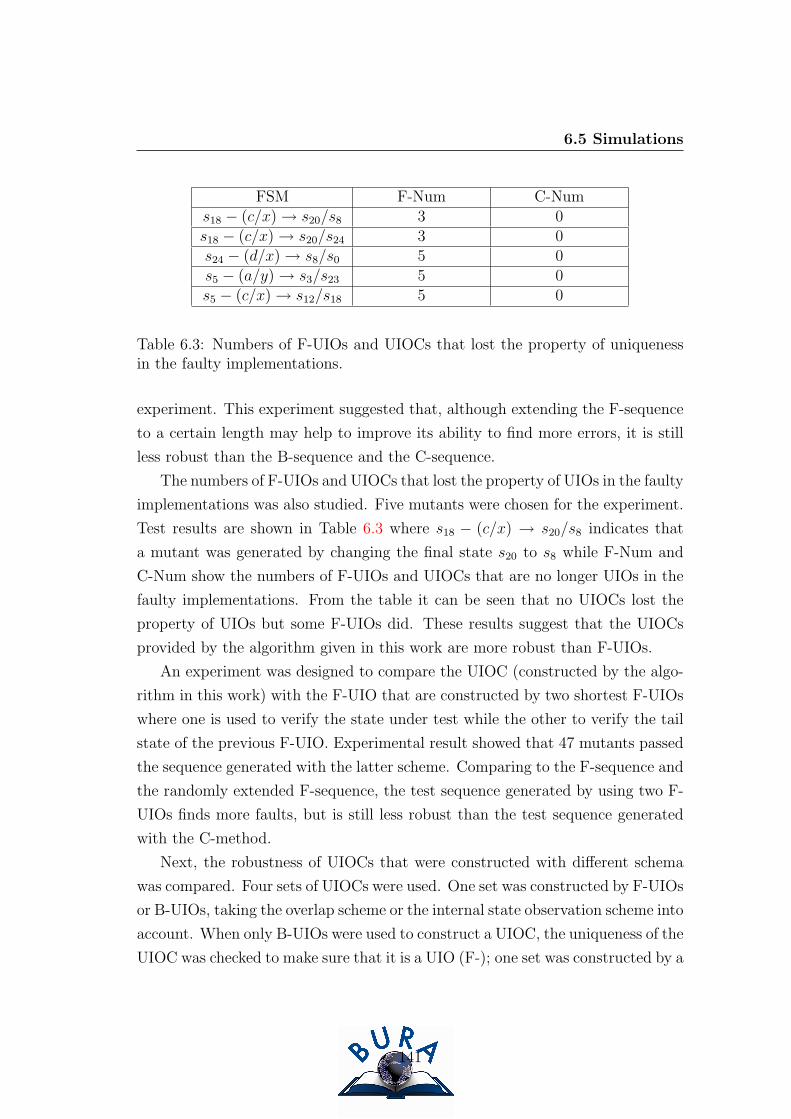
6.5 Simulations
FSM F-Num C-Nums18 − (c/x) → s20/s8 3 0s18 − (c/x) → s20/s24 3 0s24 − (d/x) → s8/s0 5 0s5 − (a/y) → s3/s23 5 0s5 − (c/x) → s12/s18 5 0
Table 6.3: Numbers of F-UIOs and UIOCs that lost the property of uniquenessin the faulty implementations.
experiment. This experiment suggested that, although extending the F-sequence
to a certain length may help to improve its ability to find more errors, it is still
less robust than the B-sequence and the C-sequence.
The numbers of F-UIOs and UIOCs that lost the property of UIOs in the faulty
implementations was also studied. Five mutants were chosen for the experiment.
Test results are shown in Table 6.3 where s18 − (c/x) → s20/s8 indicates that
a mutant was generated by changing the final state s20 to s8 while F-Num and
C-Num show the numbers of F-UIOs and UIOCs that are no longer UIOs in the
faulty implementations. From the table it can be seen that no UIOCs lost the
property of UIOs but some F-UIOs did. These results suggest that the UIOCs
provided by the algorithm given in this work are more robust than F-UIOs.
An experiment was designed to compare the UIOC (constructed by the algo-
rithm in this work) with the F-UIO that are constructed by two shortest F-UIOs
where one is used to verify the state under test while the other to verify the tail
state of the previous F-UIO. Experimental result showed that 47 mutants passed
the sequence generated with the latter scheme. Comparing to the F-sequence and
the randomly extended F-sequence, the test sequence generated by using two F-
UIOs finds more faults, but is still less robust than the test sequence generated
with the C-method.
Next, the robustness of UIOCs that were constructed with different schema
was compared. Four sets of UIOCs were used. One set was constructed by F-UIOs
or B-UIOs, taking the overlap scheme or the internal state observation scheme into
account. When only B-UIOs were used to construct a UIOC, the uniqueness of the
UIOC was checked to make sure that it is a UIO (F-); one set was constructed by a
141

6.5 Simulations
complete set of F-UIOs, without using the overlap or the internal state observation
scheme; one set was constructed by using F-UIOs and B-UIOs that can naturally
form circuits; the last was constructed by using F-UIOs and B-UIOs that cannot
form circuits. A set of transfer sequences was added to complete the circuits. The
experimental showed that 4 mutants passed the UIOC sequence generated using
F-UIOs, B-UIOs and transfer sequences; 1 passed the UIOC sequences generated
using a complete set of F-UIOs without using overlap or internal observation
scheme; 1 passed the UIOC using F-UIOs and B-UIOs without using overlap or
internal state observation scheme. The latter two sequences failed to find the
same mutant. It can be seen that test sequences generated using F-UIOs, B-
UIOs and a set of transfer sequences showed even worse test performance than
those generated with B-method. The experimental results suggest that UIOCs
constructed by the algorithm given in ref. (SL92) (using a transfer sequence to
complete the circuit) are less robust than those that were constructed by the
algorithm given in this work. Compared to the test results of the corresponding
test sequences, it can be suggested that the use of the overlap or the internal
state observation scheme is likely to make the UIOCs more robust.
We also investigated the test performance of the F-UIO, B-UIO and UIOC
methods when applied to FSMs with different numbers of states. All FSMs are
randomly generated. They are completely specified, deterministic and strongly
connected. The input set and the output set for all FSMs are {a, b, c, d} and
{x, y}. All UIOCs constructed by a complete set of B-UIOs are verified to be
F-UIOs. The result of the experiment is shown in Table 6.4. The table shows no
significant relationship between the number of states and the number of mutants
that passed the test, which indicates that the quality of testing is not only de-
termined by the test method, but also determined by the structure of systems.
But it can still be seen that, for all FSMs tested, the test sequence generated
with the C-method is better than or equal to others. In the experiments, there
are 20× 4 + 20 = 100, 400, 900, 1600, 2500, 3600, 4900 and 6400 mutants in the
FSMs with 5, 10, 15, 20, 25, 30, 35 and 40 states respectively. Therefore, the
total number of mutants in the experiments is 30390. Three mutants passed the
C-sequences, which implies that C-method achieves 99.99% fault coverage in the
experiments.
142

6.5 Simulations
States F-method B-method C-method5 0 0 010 1 1 115 1 1 020 17 8 025 199 3 030 0 0 035 156 8 140 9 2 1
Table 6.4: Mutants that pass the test.
The mutant that passed the C-sequence in the FSM with 10 states was studied.
In the implementation, transition tr14=s3 − (c/y) → s4 is mutated by changing
s4 to s3. All UIOC sequences generated from the specification FSM were then
checked for the uniqueness in the IUT. When applying the input part of the UIOC
sequence for s4, we found that both s3 and s4 produced the same output. Thus,
UIOC sequence for s4 loses the uniqueness in the IUT and fails to identify s4.
Figure 6.9 shows the sequences of transitions traversed by this UIOC sequence in
the specification FSM and the faulty implementation respectively. By examining
the structures of all UIOC sequences, we found that none of the UIOC sequence
traverses transition tr14. This determines that the faulty implementation of tr14 is
less likely to be detected in the stages of internal state verification, which reduces
the chance on finding this error. From figure 6.9 it can also be noted that the
faulty implementation of tr14 ends up at the state that is exactly the first state,
s3, that the UIOC sequence traverses when it is applied to verify s4. If the faulty
implementation of tr14 ends up at another internal state of the UIOC sequence,
the fault may be detected by the internal state verification. However, the fault
occurs before the process of internal state verification starts. Since tr14 holds the
same I/O behaviour as that of transition s4− (c/y) → s3, the fault is likely to be
masked in the C-sequence. This work did not provide solutions to overcome the
problem. Future work will address this issue.
The lengths of test sequences generated with F-, B- and C-methods were also
compared. Table 6.5 shows the lengths of test sequences for different systems. It
143

6.6 Summary
Figure 6.9: UIOC sequence for s4 in the FSM with 10 states and the faultyimplementation that causes the fault masking in the UIOC sequence.
can be seen that the sequences generated with the F-method are always shorter
than that with the B- and the C-method. However, the test sequences gener-
ated with the C-method are not always longer than those produced using the
B-method. In the majority of studies, the C-sequences were slightly longer than
the B-sequence while in some cases such as the FSM with 20 states the C-sequence
was shorter than the B-sequence.
6.6 Summary
In this chapter, we investigated the problem of fault masking in UIOs. Based
on the work of (LS92), two basic types of fault masking involving UIOs were
formalised. A new type of UIOC was proposed to overcome the two fault types.
When constructing a UIOC sequence, by further checking the tail state of a UIO,
type 1 in the faulty implementation may be avoided while by introducing the
overlap scheme and internal state observation scheme, type 2 may be avoided.
The procedure of verifying the final states of UIOs was terminated by the con-
144

6.6 Summary
States F-method B-method C-method5 88 160 9810 198 338 35115 290 484 50220 398 687 67025 506 915 101530 684 1137 112335 740 1315 133940 857 1521 1568
Table 6.5: Lengths of the test sequences.
struction of circuits where every UIO provides evidence for the correctness of the
previous UIO’s tail state.
A set of experiments was designed to study the test performance. Experimen-
tal results showed that many more faulty implementations passed the F-sequence
than the B-sequence. This suggested that the B-method was more robust than the
F-method, which is consistent with the work in ref. (SST91); meanwhile, in the
experiment, no faulty implementation passed the C-sequence, which suggested
that the C-method is more robust than the F-method and the B-method.
Performance of UIOCs constructed by the algorithm given in this paper and
in ref. (SL92) was also compared. Experimental results showed that UIOCs
constructed by the algorithm given in ref. (SL92)(using a transfer sequence to
complete a circuit) were less robust than those constructed by the algorithm given
in this paper. The experimental results also suggested that the use of the overlap
or internal state observation scheme is likely to make the UIOCs more robust.
In this work, internal state observation scheme considered the sampling of one
internal state of a UIO sequence. If a UIO sequence is comparatively long, in
order to increase the test confidence, more than one state might be considered
for observation. In future work, more studies will be proceeded to investigate the
effectiveness of internal sampling schemes.
A set of FSMs was devised to compare the test performance among different
methods. Experimental results showed that the (new) C-method was consistently
better than or equal to the F-method and the B-method. In the devised exper-
145

6.6 Summary
iments, the (new) C-method achieved more than 99.99% fault coverage. It also
showed that the C-sequences were not always longer than the B-sequences. In
the majority of studies, the C-sequences were slightly longer than the B-sequence
while in some cases, the C-sequences were shorter than the B-sequences.
However, it has also been noted that a few of the faulty implementations
passed the C-sequences in the experiments. More work needs to be carried on to
study the factors that caused the failure of C-sequences.
146

Chapter 7
Fault isolation and identification
7.1 Introduction
The process of testing aims to check whether the system being developed con-
firms to its specification. When testing from finite state machines, a set of test
sequences is usually required for conformance testing. These test sequences are
applied to the Implementation Under Test (IUT) for fault detection. I/O dif-
ferences exhibited between the IUT and its specification suggest the existence of
faults in the implementation. The first observed faulty I/O pair in an observed
input/output sequence is called a symptom. A symptom could have been caused
by either an incorrect output (an output fault) or an earlier incorrect state trans-
fer (a state transfer fault). Applying strategies to determine the location of faults
is therefore important.
Ghedamsi and Bochmann (GB92; GBD93) generate a set of transitions whose
failure could explain the behaviour exhibited. These transitions are called candi-
dates. They then produce tests (called distinguishing tests) in order to find the
faulty transitions within this set. However, in their approach, the cost of gener-
ating a conflict set is not considered. Hierons (Hie98) extended the approach to a
special case where a state identification process is known to be correct. Test cost
is then analysed by applying statistical methods. As the problem of optimising
the cost of testing is NP-hard (Hie98), heuristic optimisation techniques such as
Tabu Search (TS) and Hill Climbing (HC) are therefore suggested (Hie98).
This chapter studies fault diagnosis when testing from finite state machines.
147

7.2 Isolating single fault
The work is motivated by an interesting question described as follows. Let ts be
a test sequence of length L and let the ith input of ts, 1 ≤ i ≤ L , execute a
faulty transition trf in the IUT. The question is whether it is possible to define
the maximum number of inputs that is needed to reveal the failure (a symptom is
exhibited) after trf being executed. In other words, given a symptom exhibited
at the jth input of ts, is it possible to define an interval with a maximum range
dmax, dmax ≥ 0, such that inputs between (j− dmax)th and the jth of ts execute a
sequence of transitions that must contain trf? If such an interval can be defined,
the process of fault isolation is then reduced to that of fault identification in a
shorter test sequence.
Obviously, the smaller dmax is, the less number of transitions will be considered
when isolating the faulty transition. It is always preferred that a symptom is
observed immediately after a faulty transition is executed. However, it may
require more inputs to exhibit the fault.
Clearly, the sequence of transitions executed up to the symptom contains the
faulty transition that causes the occurrence of the symptom. However, diagnosing
within such a set of candidates might result in a high cost of fault isolation.
Finding ways to define the maximum number of inputs that is required to exhibit
an executed fault is therefore of great value for minimising the cost of fault
isolation and identification.
In this work, heuristics are proposed for fault diagnosis, which helps to reduce
the cost of fault isolation and identification. In the proposed method, a set of
transitions with minimum size is constructed to isolate the faulty transition that
could explain an observed symptom. The erroneous final state of the isolated
faulty transition is further identified by applying the proposed heuristics. The
heuristics defined in this work consider the use of the U-method (ATLU91). One
can easily extend the approach to other formal methods such as the W-method
(Cho78) and the Wp-method (FBK+91).
7.2 Isolating single fault
This section introduces an approach for detecting a single fault in the IUT and
the construction of a conflict set for fault diagnosis.
148

7.3 Minimising the size of a conflict set
7.2.1 Detecting a single fault
When testing an IUT, a set of tests TC = {tc1, tc2, ..., tcl} needs to be developed.
A test tci consists of a sequence of expected transitions 〈ti,1, ti,2, ..., ti,ni〉, starting
at s0, with input 〈xi,1, xi,2, ..., xi,ni〉 and the expected output 〈yi,1, yi,2, ..., yi,ni
〉where yi,ni
is the expected output after input xi,ni. When executed, tci produces
the observed output 〈zi,1, zi,2, ..., zi,ni〉. If differences between yi = 〈yi,1, yi,2, ..., yi,ni
〉and zi = 〈zi,1, zi,2, ..., zi,ni
〉 appear, there must exist at least one faulty transition
in the implementation. The first difference exhibited between yi and zi is called a
symptom. Additional tests are necessary in order to isolate the faulty transitions
that cause the observed symptom.
7.2.2 Generating conflict sets
A conflict set is a set of transitions, each of which could be used to explain a
symptom exhibited. Here, the work focuses on identifying the faulty transition
that is responsible for the first exhibited symptom. The transitions after the
symptom are ignored.
Suppose, for a test tci, the sequence of expected transitions is 〈ti,1, ti,2, ..., ti,ni〉
where ni is the number of transitions. When executed with 〈xi,1, xi,2, ..., xi,ni〉,
a symptom occurs at the input xi,l, the conflict set of the maximum size is
{ti,1, ti,2, ..., ti,l} where 1 ≤ l ≤ ni.
7.3 Minimising the size of a conflict set
If the number of transitions in a conflict set is large, the effort required for isolating
the fault could be high. It is therefore useful to reduce the size of a conflict set.
Two abstract schema are applied in this work, these being:
1. Transition removals using transfer sequences.
2. Transition removals using repeated states.
In the first scheme, a short transfer sequence is used to remove a segment
of inputs from the original test sequence. This may lead to a symptom being
observed in a shorter test sequence; while, in the second scheme, a segment of
149

7.3 Minimising the size of a conflict set
inputs is further removed from the original test sequence. These inputs execute
a sequence of transitions where the initial state of the first transition is the final
state of the last transition. By such an operation, a symptom might be observed
in a shorter test sequence, which helps to reduce the cost of fault isolation. Two
removal schema are discussed in the following subsections.
7.3.1 Estimating a fault location
Once a symptom is observed, the set of transitions executed up to the symptom
constitutes a conflict set Sconflict with the maximum size. A subset of transitions
Sr ⊂ Sconflict might be removed to reduce the size of Sconflict by applying some
transfer sequences. Before explaining this in detail, some concepts are defined.
Definition 7.3.1 A UIO sequence generated from the specification FSM is a
strong UIO if it can identify the corresponding state in the IUT; otherwise, it
is a weak UIO.
Due to the problem of fault masking in UIOs, a UIO sequence generated from
the specification FSM might lose its property of uniqueness and fail to identify
its corresponding state in the IUT (CVI89; Nai95).
Definition 7.3.2 When testing an IUT, if the UIOs used for the generation of
a test sequence are all strong UIOs, the test is a strong test and the test sequence
is a strong test sequence; otherwise, the test is a weak test and the test sequence
is a weak test sequence.
Definition 7.3.3 In a UIO-based test, if there are k weak UIOs in the test se-
quence, the test is called a k−degree weak test and the test sequence is a k−degreeweak test sequence.
It can be seen that a strong test is a 0− degree weak test.
Definition 7.3.4 Let [a,b] be the interval of transitions between the ath and the
bth inputs from an input sequence α. A transition tr is said to be within [a,b] of
α if the cth input executes tr when α is applied to the FSM for some a ≤ c ≤ b.
150

7.3 Minimising the size of a conflict set
In FSM-based testing, a complete test sequence should test all transitions in
the FSM M . A transition is tested by checking its I/O behaviour plus the tail
state verification. Once a transition test is finished, M arrives at a state s. If s is
not the initial state s′of the transition selected for the following test, a transfer
sequence is required to move the M to s′. This transfer sequence constitutes a
linking sequence in the final test sequence.
Definition 7.3.5 A linking sequence in a test sequence for an FSM M is a trans-
fer sequence that moves M to the initial state of a transition under test after the
previous transition test is finished.
Proposition 7.3.1 In a UIO-based test, if the test is a strong test and a symptom
is observed at the ath input, then the faulty transition that causes the occurrence
of the symptom must be within [(a-LUIO(max)-LLink(max)), a] of the inputs where
LUIO(max) is the max length of UIOs and LLink(max) the max length of linking
sequences.
Proof: The standard strategy of a transition test in UIO-based test is formed by
a transition I/O test and the tail state verification. Since the test is a strong
test, no problem of fault masking exists in the test sequence. Suppose a faulty
transition is executed at the bth input and the fault is unveiled with an observable
symptom at the ath input. If the transition has an I/O error, the fault is detected
by the bth input (a = b); otherwise, if the transition is one under test, the faulty
final state is detected by the following state verification with maximum length
LUIO(max) (b ≤ a ≤ b + LUIO(max)), or, if the faulty transition is an element of a
linking sequence, the following inputs move the machine to the initial state of the
next transition under test with the max steps of LLink(max). After executing the
transition with one input, the faulty final state can be detected by the forthcoming
state verification with the max steps of LUIO(max) (b ≤ a ≤ b + LLink(max) + 1 +
LUIO(max)). Therefore, if a symptom is observed by a strong test sequence at the
ath input, the faulty transition that caused the occurrence of the symptom must
be within [(a− LUIO(max) − LLink(max)), a] of the inputs. �
151

7.3 Minimising the size of a conflict set
Definition 7.3.6 In a weak test, if a UIO sequence fails to identify the corre-
sponding state in the IUT more than once, the problem is called fault masked UIO
cycling.
Figure 7.1: Fault Masked UIO Cycling
An example of fault masked UIO cycling is illustrated in Figure 7.1 where a
state transfer error occurs in t1(si → sj) first, leading to an erroneous final state
sx. Due to fault masking, the UIO of sj fails to find the error, moving the FSM
to sz. Suppose, according to the test order, t2(sk → sj) is tested after t1. When
responding to the input, the IUT produces the same output as defined in the
specification and arrives at sx. When applying the UIO of sj, it again fails to
find the fault. The UIO of sj appears in the test twice, in both cases, failing to
exhibit an incorrect final state in the observed input/output sequence.
Proposition 7.3.2 In a k − degree weak test, if the problem of fault masked
UIO cycling does not exist and a symptom is observed at the ath input, then the
faulty transition that causes the occurrence of the symptom must be within [(a+1-
(k+ 1) ∗ (LUIO(max)+LLink(max)+1)), a] of the inputs where LUIO(max) is the max
length of UIOs and LLink(max) the max length of linking sequences.
Proof: Similar to Proposition 7.3.1, proof can be obtained by considering the test
structure. Since no problem of fault masked UIO cycling exists in the test, if
there are k weak UIOs in the test, the faulty final state of a faulty transition can
be detected with the maximum steps of (k + 1) ∗ (LUIO(max) + LLinking(max) + 1).
�
152
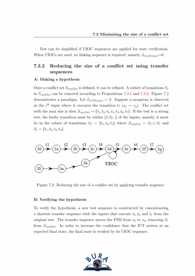
7.3 Minimising the size of a conflict set
Test can be simplified if UIOC sequences are applied for state verification.
When UIOCs are used, no linking sequence is required, namely, LLink(max)=0.
7.3.2 Reducing the size of a conflict set using transfersequences
A: Making a hypothesis
Once a conflict set Sconflict is defined, it can be refined. A subset of transitions Sr
in Sconflict can be removed according to Propositions 7.3.1 and 7.3.2. Figure 7.2
demonstrates a paradigm. Let LUIO(max) = 2. Suppose a symptom is observed
at the ith input where it executes the transition t7 (sf → sg). The conflict set
with the max size is then Sconflict = {t1, t2, t3, t4, t5, t6, t7}. If the test is a strong
test, the faulty transition must be within [(i-3), i] of the inputs, namely, it must
be in the subset of transitions Sf = {t5, t6, t7} where Sconflict = Sf ∪ Sr and
Sr = {t1, t2, t3, t4}.
Figure 7.2: Reducing the size of a conflict set by applying transfer sequence
B: Verifying the hypothesis
To verify the hypothesis, a new test sequence is constructed by concatenating
a shortest transfer sequence with the inputs that execute t5, t6 and t7 from the
original test. The transfer sequence moves the FSM from s0 to sd, removing Sr
from Sconflict. In order to increase the confidence that the IUT arrives at an
expected final state, the final state is verified by its UIOC sequence.
153

7.3 Minimising the size of a conflict set
When the new test sequence is applied to the system, two observations need to
be made: 1. have any failures been observed from applying the transfer sequence
in the new test sequence? 2. if no failure is exhibited by the transfer sequence,
the input/output pairs observed afterwards in the new test sequence need to be
compared to those observed after sd in the original test to check if there exist any
differences. If a failure is observed by applying the transfer sequence, transitions
executed by the transfer sequence constitutes a new conflict set S′
conflict and
additional tests need to be developed to isolate the fault. Since the transfer
sequence traverses the shortest path from s0 to sd, |S′
conflict| ≤ |Sconflict|.Let tr
′
f be the faulty transition that is identified in S′
conflict. If tr′
f ∈ Sconflict,
tr′
f is defined as the principal faulty transition that causes the occurrence of
the observed symptom in the original test. The process of isolating the faulty
transition for the observed symptom is then complete. More faults might exist
in Sconflict, these faults can be isolated by constructing some new test sequences
where tr′
f is not executed or is executed as late as possible; otherwise, if tr′
f /∈Sconflict, one more fault is detected. tr
′
f needs to be further processed as described
in Section 7.4.2. Meanwhile, a new transfer sequence needs to be constructed until
no failure is exhibited by this sequence.
Suppose, after applying the transfer sequence, no I/O change is found when
the sequence of transitions in Sf is executed, it provides evidence that both the
transfer sequence and the input sequence that executes Sr in the original test
make the FSM arrive at the same state scom. Since the final state of the transfer
sequence is verified by its UIOC sequence, evidence that scom = sd is provided as
well. This further suggests that Sf contains the faulty transition that causes the
symptom. Additional tests need to be developed to identify the faulty transition.
Having tested all transitions in Sconflict, if no faulty transition is defined, it
implies that at least one UIO fails to identify the corresponding state. The test
is a weak test. Proposition 2 can be applied to estimate the input interval that
the faulty transition might fall in. The process starts by considering [(i+1− (k+
1) ∗ (LUIO(max) + LLink(max) + 1)), i]|k=1 first. By removing a set of transitions, if
the faulty transition is still not isolated, k is increased by 1. The process repeats
until the faulty transition is isolated.
154
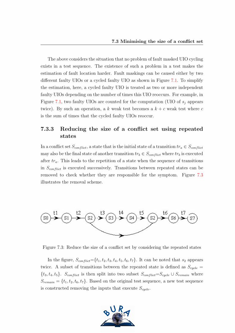
7.3 Minimising the size of a conflict set
The above considers the situation that no problem of fault masked UIO cycling
exists in a test sequence. The existence of such a problem in a test makes the
estimation of fault location harder. Fault maskings can be caused either by two
different faulty UIOs or a cycled faulty UIO as shown in Figure 7.1. To simplify
the estimation, here, a cycled faulty UIO is treated as two or more independent
faulty UIOs depending on the number of times this UIO reoccurs. For example, in
Figure 7.1, two faulty UIOs are counted for the computation (UIO of sj appears
twice). By such an operation, a k weak test becomes a k + c weak test where c
is the sum of times that the cycled faulty UIOs reoccur.
7.3.3 Reducing the size of a conflict set using repeatedstates
In a conflict set Sconflict, a state that is the initial state of a transition tra ∈ Sconflict
may also be the final state of another transition trb ∈ Sconflict where trb is executed
after tra. This leads to the repetition of a state when the sequence of transitions
in Sconflict is executed successively. Transitions between repeated states can be
removed to check whether they are responsible for the symptom. Figure 7.3
illustrates the removal scheme.
Figure 7.3: Reduce the size of a conflict set by considering the repeated states
In the figure, Sconflict={t1, t2, t3, t4, t5, t6, t7}. It can be noted that s2 appears
twice. A subset of transitions between the repeated state is defined as Scycle =
{t3, t4, t5}. Sconflict is then split into two subset Sconflict=Scycle ∪ Sremain where
Sremain = {t1, t2, t6, t7}. Based on the original test sequence, a new test sequence
is constructed removing the inputs that execute Scycle.
155

7.4 Identifying a faulty transition
Applying the new test sequence to the system, if, when compared to the
original test, the rest of the I/O behaviour remains unchanged, the symptom is
then observed in a shorter sequence. The conflict set is consequently reduced to
Sremain. Additional tests can then be devised to verify the hypothesis.
If, compared to the corresponding I/O segment in the original test sequence,
the new test sequence behaves differently, no conclusion can be drawn and, in
this situation, the removal scheme of using repeated states does not reduce the
size of Sconflict.
7.4 Identifying a faulty transition
Having reduced the size of a conflict set, further tests need to be devised to identify
the fault. Here, the process intends not only to locate the faulty transition, but
also to determine its faulty final state.
7.4.1 Isolating the faulty transition
After a conflict set Sconflict has been minimised, in order to locate the faulty
transition, transitions in Sconflict need to be tested individually. Each transition
tri ∈ Sconflict is tested by moving the FSM to the head state of tri, executing tri
and then verifying tri’s tail state. In order to increase the reliability, this process
should avoid using other untested candidates in Sconflict.
If, when testing a transition tri ∈ Sconflict, the use of another untested candi-
date trj ∈ Sconflict is inevitable, one might verify trj’s tail state as well when it
is executed and then apply a transfer sequence to move the IUT back to the tail
state of trj. If there exists a UIOC sequence for the tail state of trj, the UIOC
sequence can be applied. Through such an operation, two transitions are tested
simultaneously.
The test process described above assumes that UIOs or UIOCs used for state
verification are strong UIOs. This, however, might not be true. In order to
increase test confidence, one might use a set of test sequences to test a transition
tri ∈ Sconflict, each of which uses a different UIO sequence to verify the final state
of tri. This, however, requires more test efforts.
156

7.4 Identifying a faulty transition
7.4.2 Identifying the faulty final state
Once a faulty transition has been located, the faulty final state needs to be
identified. This helps to reduce the fault correction effort. A set of estimated
erroneous final states SEndState is then constructed.
Let n be the number of states in the FSM. Suppose transition trf : si → sj is
identified as being faulty. It can be noted that, in terms of the alternative final
states for trf , there are n−1 possible mutants. Therefore, SEndState with the max
size is SEndState = {s1, ..., sj−1, sj+1, ..., sn} and |SEndState| = n− 1.
The size of SEndState might be reduced by comparing the I/O behaviour ex-
hibited after the faulty transition in the IUT to that defined in the specification.
Definition 7.4.1 Let MS = (I, O, S, δ, λ, s0) be a specification FSM and MI =
(I, O, S, δ′, λ
′, s0) be an implementation FSM of MS. Let xv ∈ I be an input
that executes a transition tr from sa to sb in MI and zv be the observed output,
zv = λ′(sa, xv). SV DIS ⊆ S is called the valid defined initial state (VDIS) set of
xv/zv if zv ∈ O, ∀sv ∈ SV DIS, λ(sv, xv) = zv and ∀sv /∈ SV DIS, λ(sv, xv) 6= zv.
Let xv be the input that executes the transition following the isolated faulty
transition trf in the IUT and zv be the observed output. The set SV DIS of xv/zv is
constructed by applying xv to each state in the specification FSM and comparing
the corresponding output with zv. Let yv(i) be the response from the specification
FSM when the machine is in si ∈ S and receives xv. By comparing yv(i) to
zv, S can be divided into two subsets SV DIS and SV DIS where ∀sj ∈ SV DIS,
λ(sj, xv) = yv(j)= zv and ∀sk ∈ SV DIS, λ(sk, xv) = yv(k)
6= zv. If SV DIS 6= ∅, it
indicates there exists a non-empty set of states SV DIS such that ∀sk ∈ SV DIS,
λ(sk, xv) 6= zv, which suggests that the erroneous final state of trf is less likely to
be in SV DIS. SEndState is then reduced to SV DIS.
The size of the estimated faulty final state set might be further reduced by
using a set of faulty final state identification test sequences.
Definition 7.4.2 Let I = {a1, ..., ak} be the input set of a specification FSM MS
and MI be an IUT of MS. Let an isolated faulty transition trf of MI be executed
by a test sequence tv = x1, ..., xv at the vth input xv. TS = {ts1, ..., tsk} is called
157

7.5 A case study
the set of faulty final state identification test sequences (FFSITSs) of trf where1tsl = tv · al, al ∈ I.
For each tsj ∈ TS, a set SV DIS can be constructed when aj is applied to the
IUT, denoted by SjV DIS. The final estimated faulty final state set SEndState can
then be reduced to SEndState = S1V DIS ∩ ... ∩ Sk
V DIS.
The complexity of faulty final state identification is determined by the number
of states in SEndState. This is discussed in Section 7.6.2. If the size of SEndState is
reduced, the effort involved in identifying the faulty final state is thus reduced.
Once the size of SEndState is reduced, each state si ∈ SEndState needs to be
tested to identify the faulty final state. si is checked by moving the IUT from s0
to si with a transfer sequence Seq(transfer), and then applying UIOsifor si. In
order to increase test confidence, a set of test sequences, TV = {tv1, tv2, ..., tvr},can be applied where tvi ∈ TV is constructed by concatenating Seq(transfer) with
a different UIO sequence for si.
7.5 A case study
A case study is designed to evaluate the effectiveness of the proposed method.
A reduced, completely specified and strongly connected specification FSM M is
defined in Table 7.1 where the machine has five states. The input set is I =
{a, b, c, d} and output set O = {x, y}. In order to simplify the analysis, a set
of UIOCs (shown in Table 7.2) is used for state verification. For each state, the
first UIOC sequence is used for the generation of the test sequence. The rest of
the UIOCs are used to verify hypotheses when diagnosing faults. The 2maximum
length of UIOCs, LUIO(max), is 4. In the implementation M′, two faults are
injected. They are listed in Table 7.3.
Based upon rural Chinese postman algorithm and UIOCs for state verifica-
tion, a test sequence ts is generated from M . ts is then applied to M′for fault
detection.
1Notation “·” implies the concatenation of two sequences2Here, LUIO(max) refers to the maximum length of UIOCs that are used for the test gener-
ation.
158

7.5 A case study
No Transition No Transition
t1 s0a/x−−−→ s1 t11 s2
c/x−−−→ s3
t2 s0d/y−−−→ s2 t12 s2
b/y−−−→ s4
t3 s0c/x−−−→ s3 t13 s3
a/x−−−→ s0
t4 s0b/y−−−→ s4 t14 s3
b/y−−−→ s1
t5 s1d/y−−−→ s0 t15 s3
c/x−−−→ s2
t6 s1a/y−−−→ s2 t16 s3
d/y−−−→ s4
t7 s1c/x−−−→ s3 t17 s4
b/x−−−→ s0
t8 s1b/x−−−→ s4 t18 s4
d/y−−−→ s1
t9 s2d/x−−−→ s0 t19 s4
c/x−−−→ s2
t10 s2a/y−−−→ s1 t20 s4
a/y−−−→ s3
Table 7.1: Specification finite state machine used for experiments
After ts is applied to M′, a symptom is observed at the 17th input where,
according to M , t8 : s1b/x−−−→ s4 should have been executed (shown in Figure
7.4). The sequence of transitions, 〈t1, t8, t19, t10, t6, t9, t1, t6, t11, t14, t8, t20, t16, t17,t2, t10, t8〉, executed by the first 17 inputs constitutes the conflict set of the max-
imum size, this being Sconflict = {t1, t8, t19, t10, t6, t9, t11, t14, t20, t16, t17, t2}.The size of Sconflict is then reduced by applying the proposed heuristics. At
first it is assumed that ts is a strong test sequence. The removal scheme is then
determined by Proposition 7.3.1. As LLink(max) = 0 and LUIO(max) = 4, according
to Proposition 7.3.1, the faulty transition that causes this symptom must be
within [13,17] of the inputs. This hypothesis reduces Sconflict to {t16, t17, t2, t10, t8}.To verify the hypothesis, a shortest transfer sequence, c/x, is applied to move
M′
from s0 to s3, removing the inputs in the original test sequence that suc-
cessively execute 〈t1, t8, t19, t10, t6, t9, t1, t6, t11, t14, t8, t20〉. The final state of the
transfer sequence s3 is afterwards verified by its UIOC sequence. In order to
increase test confidence, two UIOC sequences dada/yyyy and bba/yxy for s3 are
applied. After applying cbba and cdada to M′, xyxy and xyyyx (xyyyx 6= xyyyy)
are received respectively. These results imply that (1) t3 is faulty. It is detected
by dada/yyyy but masked by bba/yxy; or, (2) t3 is correctly implemented but
159

7.5 A case study
State UIOC sequences0 dd/yx
daad/yyyxs1 bca/xxy
baca/xyxys2 daa/xxy
dadd/xxyys3 bba/yxy
dada/yyyys4 bdab/xyyx
aaab/yxxx
Table 7.2: Unique input/output circuit sequences for each state of the finite statemachine shown in Table 7.1.
No Transition Mutant
t3 s0c/x−−−→ s3 s0
c/x−−−→ s0
t17 s4b/x−−−→ s0 s4
b/x−−−→ s4
Table 7.3: Injected faults
dada/yyyy traverses a faulty transition, leading to a failure being observed.
To further check the hypothesis, two additional tests tv1 = (c/x)·(aaba/xxxy)and tv2 = (c/x) · (abdba/xyyxy) are devised where aaba/xxxy and abdba/xyyxy
are two different UIOC sequences for s3. After applying caaba and cabdba to M′,
xxyyy and xxxyxy are received, xxyyy 6= xxxxy and xxxyxy 6= xxyyxy, which
suggests t3 is faulty and bba/yxy is a weak UIO for s3.
The erroneous final state of t3 is further identified as described in Section 7.4.
A set of estimated faulty final states for t3 is constructed by applying a set of
faulty final state identification test sequences to M′, each test sequence in the set
being used to construct the corresponding SV DIS.
Let Sg/hV DIS be the SV DIS of g/h where g/h indicates that, when applying g to
M′, h is observed. After all elements in the input set have been applied, a set
of SV DIS can then be obtained. The elements in the set are Sa/xV DIS = {s0, s3},
Sb/yV DIS = {s0, s2, s3}, Sc/x
V DIS = {s0, s1, s2, s3, s4} and Sd/yV DIS = {s0, s1, s3, s4}. The
160

7.5 A case study
Figure 7.4: Fault detection and identification in M′
final estimated faulty final state set is SEndState = Sa/xV DIS∩S
b/yV DIS∩S
c/xV DIS∩S
d/yV DIS
= {s0, s3}. Additional tests can now be added to verify the hypothesis.
In order to increase test confidence, two test sets tvs0 = {(c/x) · (dd/yx),
(c/x) · (daad/yyyx)} and tvs3 = {(c/x) · (aaba/xxxy),(c/x) · (dada/yyyy)} are
devised where s0 and s3 are tested respectively. In both tests, two different
UIOC sequences are used to verify the corresponding final state. The test results
suggest that the erroneous final state of t3 is s0.
Since t3 /∈ Sconflict, a new transfer sequence needs to be constructed to isolate
the fault that causes the failure observed in the original test. Still, the Sconfilict
is assumed to be {t16, t17, t7, t10, t8}. Transfer sequence dc/yx is applied, moving
M′
from s0 to s3. In order to increase test confidence, two UIOC sequences,
aaba/xxxy and dada/yyyy, are used to verify s3.
After dcaaba and dcdada are applied to M′, yxxxxy and yxyyyy are received
respectively. This provides evidence that the current state is s3. Continue to ap-
ply those inputs in the original test sequence after the 17th input. By comparing
the behaviour to the original test, it is found that the outputs remain unchanged.
This increases confidence that the conflict set Sconflict = {t16, t17, t7, t10, t8} con-
tains the faulty transition that cause the observed symptom. Additional tests are
required to check each transition in Sconflict.
161

7.5 A case study
When constructing a test sequence, the traversing of t3 needs to be avoided
since it has been found to be faulty.
A set of tests, V T = {vtt16 , vtt17 , vtt2 , vtt10 , vtt8} is devised where vtt16 , vtt17 ,
vtt2 , vtt10 and vtt8 check t16, t17, t2, t10 and t8 respectively. In order to increase
test confidence, each test in V T is comprised of two test sequences where two
different UIOCs are used to verify the corresponding tail state. These tests are
Transition Test Sett16 vtt16 = {(ac/xx) · (d/y) · (bdab/xyyx), (ac/xx) · (d/y) · (aaab/yxxx)}t17 vtt17 = {(b/y) · (b/x) · (dd/yx), (b/y) · (b/x) · (daad/yyyx)}t2 vtt2 = {(a/x) · (c/x) · (daa/xxy), (a/x) · (c/x) · (dadd/xxyy)}t10 vtt10 = {(d/y) · (a/x) · (bca/xxy), (d/y) · (a/x) · (baca/xyxy)}t8 vtt8 = {(a/x) · (b/x) · (bdab/xyyx), (a/x) · (b/x) · (aaab/yxxx)}
When applying vtt2 and vtt10 to M′no failure is observed, which suggests t2
and t10 are correctly implemented. When applying vtt17 toM′both test sequences
exhibit a failure which suggests t17 is faulty.
When applying vtt16 and vtt8 to M′, in both tests, one test sequence exhibits
a failure while the other shows no error. The test results are {(ac/xx) · (d/y) ·(bdab/xyyy), (ac/xx) ·(d/y) ·(aaab/yxxx)} and {(a/x) ·(b/x) ·(bdab/xyyy), (a/x) ·(b/x) · (aaab/yxxx)}. Through these observations, two hypotheses can be made:
(1) t8 and t16 are faulty, and aaab/yxxx is a weak UIO sequence for s4. A fault
is exhibited by bdab/xyyx but masked by aaab/yxxx; (2) t8 and t16 are correctly
implemented, but bdab/xyyx traverses at least one faulty transition, leading to a
failure being observed.
By examining the structure of bdab/xyyx, it is found that bdab/xyyx tra-
verses t17 that is found to be faulty. It is likely that the second hypothesis is
true. To verify the hypothesis, vtt16 and vtt8 are replaced with {(ac/xx) · (d/y) ·(abdb/yyyy), (ac/xx) ·(d/y) ·(acab/yxyy)} and {(a/x) ·(b/x) ·(abdb/yyyy), (a/x) ·(b/x)·(acab/yxyy)}. In the tests, (abdb/yyyy) and (acab/yxyy) are two UIOC se-
quences for s4 where, according toM , t17 is not traversed. After applying acdabdb,
acdacab, ababdb and abacab to M′, xxyyyyy, xxyyxyy, xxyyyy and xxyxyy are
received respectively. These results suggest that t8 and t16 have been correctly
implemented.
162
7.6 Complexity
The faulty final state of t17 is then identified. After all elements in the input
set being applied, a set of SV DIS is obtained, this being: Sa/yV DIS = {s1, s2, s4},
Sb/xV DIS = {s1, s4}, Sc/x
V DIS = {s0, s1, s2, s3, s4} and Sd/yV DIS = {s0, s1, s3, s4}. The
final estimated faulty final state set is SEndState = S0V DIS∩S1
V DIS∩S2V DIS∩S3
V DIS
= {s1, s4}. Additional tests are then devised to verify the hypothesis.
Two test sequences ts1 = (a/x) · (baca/xyxy) and ts2 = (b/y) · (aaab/yxxx)are devised where ts1 tests s1 while ts2 checks s4. It is concluded that the faulty
final state of t17 is s4.
7.6 Complexity
In this section, the complexity of the proposed approach is analysed. The analysis
is comprised of two parts - the complexity of fault isolation and the complexity
of fault identification. It is shown that the proposed approach can isolate and
identify a single fault in low order polynomial time.
7.6.1 Complexity of fault isolation
The complexity of fault isolation is determined by the strength of the UIOs used
for the generation of test sequences. The strength of a UIO is its capability to
resist fault maskings when required for state verification in the IUT (Nai95). If
a symptom is exhibited by a strong test sequence, the conflict set Sconflict is of
the maximum number |Sconflict|max = LUIO(max) + LLinking(max) + 1; otherwise, if
the test is a k weak test, |Sconflict|max = (k+ 1)× (LUIO(max) +LLinking(max) + 1),1k ≥ 0. If there exists the problem of faulty masked UIO cycling, the test is
treated as a k + c weak test as discussed in the previous sections.
After the conflict set Sconflict is constructed, in order to isolate the faulty
transitions, each transition tri ∈ Sconflict needs to be tested. Let TrS be a set
of transfer sequences where trsi ∈ TrS is used to move the IUT from s0 to the
initial state of tri ∈ Sconflict. Let LTrS(max) be the maximum length of the transfer
sequences in TrS. The maximum number of steps required for isolating a faulty
transition is of O(|Sconflict| × (LTrS(max) + LUIO(max) + 1)).
1k = 0 is equivalent to the case where the test is a strong test.
163

7.6 Complexity
The process of fault isolation from Sconflict considers the use of one UIO se-
quence for state verification when testing a transition tri ∈ Sconflict and assumes
this UIO sequence is a strong UIO. However, this might not be true. In order to
increase test confidence, a set of test sequences TSi might be used for the test of
a transition tri in Sconflict, each of which uses a different UIO sequence to verify
the final state of tri.
Let |TSi|max = m, m ≥ 1. The maximum number of steps required for
isolating a faulty transition is then of O(|Sconflict|×m× (LTrS(max) +LUIO(max) +
1)). Therefore, the maximum number of steps required for isolating a single fault
is of O((k+c+1)×(LUIO(max)+LLinking(max)+1)×m×(LTrS(max)+LUIO(max)+1))
where k is the number of faulty UIOs in the test sequence and c is the sum of
times that the cycled faulty UIOs reoccur.
7.6.2 Complexity of fault identification
A: Construction of SEndState
When identifying the faulty final state of an isolated faulty transition (if the tran-
sition holds a state transfer error), a set of estimated faulty final states SEndState
needs to be constructed by applying a set of faulty final state identification test
sequences. Suppose, in the original test, the faulty transition and the sequence
of transitions before this transition are executed by a test segment of length Lsg.
The number of steps required to construct SEndState is of O((|I| − 1)(Lsg + 1))
where I is the input set of the FSM. In order that the faulty final state is identi-
fied, each state in SEndState needs to be tested.
B: Determining the faulty final state
Let trsshortest with length Ltrs be the shortest transfer sequence that moves the
IUT from s0 to the initial state of trf . Let |SEndState| = q, 1 ≤ q ≤ |S| − 1. si ∈SEndState is checked by applying trsshortest, executing trf with the corresponding
input and applying UIOsi. The length of UIOsi
is less than or equal to LUIO(max).
The maximum number of steps required to test si ∈ SEndState is of O(Ltrs +
LUIO(max) +1). All states in SEndState need to be tested. Therefore, the maximum
164

7.7 Summary
number of steps required to identify the faulty final state in SEndState is of O(q×(Ltrs + LUIO(max) + 1)).
Again, the process of faulty final state estimation considers the use of one UIO
sequence to verify the corresponding state and assumes this UIO sequence is a
strong UIO. In order to increase test confidence, a set of distinct UIOs, MUIOi,
may be used to verify state si in SEndState. Let |MUIOi|max = p, p ≥ 1. The
maximum number of steps required to identify the faulty final state in SEndState
is then of O(q × p× (Ltrs + LUIO(max) + 1)).
By considering the process of the construction of SEndState together, the max-
imum number of steps required to identify the faulty final state is of O((|I| −1)(Lsg + 1) + q× p× (Ltrs +LUIO(max) + 1)). In the worst case where q = |S| − 1,
the maximum number of steps is of O((|I| − 1)(Lsg + 1) + p× (|S| − 1)× (Ltrs +
LUIO(max) + 1)), while, in the best case where q = 1, the maximum number of
steps is of O((|I| − 1)(Lsg + 1) + p× (Ltrs + LUIO(max) + 1)).
7.7 Summary
This chapter investigated fault diagnosis when testing from finite state machines
and proposed heuristics to optimise the process of fault isolation and identifi-
cation. In the proposed approach, a test sequence is first constructed for fault
detection. Once a symptom is observed, additional tests are designed to identify
the faults that are responsible for the occurrence of the observed symptom.
Based upon the original test, the proposed heuristics are applied to lead to a
detected symptom being observed in some shorter test sequences. These shorter
test sequences are then used for the construction of a set of diagnosing candidates
that is of the minimal size. The minimal set of candidates helps to reduce the
cost of fault isolation and identification.
The complexity of the proposed approach was described. A case study was
used to demonstrate the application of the approach. In the case study, two state
transfer faults were injected into the implementation. These faults were isolated
and identified after applying the proposed heuristics.
The case study used in this work considered the use of a comparatively simple
example for fault isolation and identification. It is shown how more complicated
165

7.7 Summary
testing problems such as k degree weak test and fault masked UIO cycling can
be catered for. However, more work is required to evaluate these approaches
experimentally. This remains a topic for future work.
166

Chapter 8
Conclusions and future work
Finite State Machines (FSMs) have been considered as powerful means in system
modelling and testing. The reviewed literature shows that, once a system is
modelled as a finite state machine, it is easy to automate the process of test
generation.
This thesis studies the automated generation of test sequences when testing
from finite state machines. Three research issues that are highly related to fi-
nite state machine based testing were investigated, these being construction of
Unique Input/Output (UIO) sequences using Metaheuristic Optmisation Tech-
niques (MOTs), fault coverage in finite state machine based testing, and fault
diagnosis when testing from finite state machines.
In the studies of the construction of UIOs, a model is proposed where a fitness
function is defined to guide the search for input sequences that are potentially
UIOs. In the studies of the improved fault coverage, a new type of Unique
Input/Output Circuit (UIOC) sequence is defined. Based upon Rural Chinese
Postman Algorithm (RCPA), a new approach is proposed for the construction of
more robust test sequences. In the studies of fault diagnosis, heuristics are defined
that attempt to lead failures to be observed in some shorter test sequences, which
helps to reduce the cost of fault isolation and identification.
The proposed approaches and techniques were evaluated with regard to a set
of case studies, which provides experimental evidence for their efficacy.
167

8.1 Contributions
8.1 Contributions
The declared contributions of this PhD work are summarised as follows:
• proposed a model for the construction of (multiple) UIOs using MOTs (see
chapter 5);
• investigated fault coverage when testing from finite state machines and pro-
posed a new method for the generation of more robust test cases (see chapter
6);
• proposed an algorithm for the construction of backward unique input/output
sequences (see chapter 6);
• studied fault diagnosis when testing from finite state machines and proposed
a set of heuristic rules for fault isolation and identification (see chapter 7).
8.2 Finite state machine based testing
Testing from finite state machines has been discussed in this thesis. It has been
demonstrated that finite state machines can be used, not only in the generation
of test sequences, but also in the control of the testing process.
Some reviewed work shows how an efficient test sequence can be generated
from the finite state machine specification. Based upon rural Chinese postman
algorithm, Aho et al. (ATLU91) showed that an efficient test sequence may be
produced using UIOs for state verification. Shen et al. (SLD92) extended the
method by using multiple UIOs for each state and showed that this leads to a
shorter test sequence. These works, however, do not consider the overlap effect
in a test sequence.
Yang et al. (YU90) and Miller (MP93) showed that overlap can be used
in conjunction with (multiple) UIOs to further reduce the test sequence length.
Hierons (Hie96; Hie97) represented overlap by invertible sequences. All of the
algorithms guarantee the construction of a test sequence in polynomial time,
which makes the finite state machines practical models for testing.
168

8.3 Construction of UIOs
8.3 Construction of UIOs
A very important issue in finite state machine based testing is the construction
of Unique Input/Output (UIO) sequences. In finite state machine based testing,
the standard test strategy defines that the tail state of a transition needs to be
verified once the I/O check is finished. UIOs are often used for state verification.
A prerequisite for UIO based testing is that we have at least one UIO sequence for
each state of the machine under test. Finding ways to construct UIOs is therefore
important.
However, computing UIOs is NP-hard (LY94). Some approaches have been
proposed for the construction of UIOs, but they all have some drawbacks. In
this work, a model is proposed for the construction of multiple UIOs using Meta-
heuristic Optimisation Techniques (MOTs), with the sharing techniques. A fit-
ness function, based on properties of a state splitting tree, guides the search for
UIOs. A sharing technique is introduced to maintain the diversity in a population
by defining a mechanism that measures the similarity of two sequences.
Two finite state machines are used to evaluate the effectiveness of a Genetic
Algorithm (GA), GA with sharing, and Simulated Annealing (SA) with sharing.
Experimental results show that, when sharing techniques are applied, both GA
and SA can find the majority of UIOs from the models under test. This result
suggests that it is possible to construct UIOs using MOTs.
8.4 The improved fault coverage
In finite state machine based testing, the problem of fault masking in unique
input/output sequences may degrade the test performance of UIO based testing.
Two basic types of fault masking are defined in (LS92). Based upon this study,
in this work, a new type of Unique Input/Output Circuit (UIOC) sequence is
proposed for state verification, which may help to overcome the drawbacks that
exist in the UIO based techniques.
UIOCs themselves are particular types of UIOs where the ending states are the
same as their initial states. When constructing a UIOC, by further checking the
tail state and by using overlap or internal state observation scheme, the abilities
169

8.5 Fault diagnosis
of UIOs to resist the problem of fault masking is enhanced. Based upon rural
Chinese postman algorithm (RCPA), a new approach for the generation of test
sequence from finite state machines is proposed.
The proposed approach was compared with the existing approaches such as
F-method and B-method by devising a set of experiments. Experimental results
suggest that the proposed approach outperforms or is equal to the existing meth-
ods.
It has also been shown that the length of the test sequence generated by
using the proposed methods is not always longer than those generated by using
the existing methods. In the majority of studies, the test sequences generated by
using the proposed method were slightly longer than those generated by using
the existing methods. However, in some cases, the proposed method results in
some shorter test sequences.
8.5 Fault diagnosis
When testing from finite state machines, a failure observed in the Implementation
Under Test (IUT) is called a symptom. A symptom could have been caused by an
earlier state transfer failure. Transitions that may be used to explain the observed
symptoms are called diagnosing candidates. Finding strategies to generate an
optimal set of diagnosing candidates that could effectively identify faults in the
IUT is of great value in reducing the cost of system development and testing.
In this work, we investigated fault diagnosis when testing from finite state
machines and propose heuristics for fault isolation and identification. The pro-
posed heuristics attempt to lead a symptom to be observed in some shorter test
sequences, which helps to reduce the cost of fault isolation and identification.
A case study was designed to investigate the effectiveness of the proposed
method. In the example, two faults were injected to the implementation under
test. These faults were identified after applying the proposed heuristics.
170

8.6 Future work
8.6 Future work
Three research issues have been investigated. In each case, we have noted some
problems. In the studies of the construction of UIOs with MOTs, by applying
sharing techniques, a genetic population is forced to form several sub-populations,
each of which aims to explore UIOs that are determined as local optima. However,
a problem was noted where the distribution of UIOs in a sub-population did
not form a good shape. The distribution of the sub-population was dominated
by several individuals. In the future work, a new encoding approach might be
considered to overcome such a problem.
In the studies of UIOC based testing, overlap and internal state sampling
schema were proposed to overcome the problem that a fault is masked by some
internal state of a UIO sequence. The study of internal state sampling scheme
considered the sampling of one state. The effectiveness of the internal sampling
scheme may be further investigated in the future work by considering the use of
more than one internal state. Meanwhile, in the experiments, test sequences gen-
erated by using the proposed method failed to detect a small number of mutants
in some devised finite state machines. The failure of fault detection in UIOC
based testing needs to be further studied.
In the studies of fault diagnosis in finite state machine based testing, heuristics
were defined that attempt to lead failures to be observed in some shorter test
sequences, which helps to reduce the cost of fault isolation and identification.
However, the example studied in the work are comparatively simple. Some more
complicated testing problems such as k degree weak test and fault masked UIO
cycling were only analytically explained but have not been studied by using some
examples. These issues need to be investigated in the future work.
171

References
[AAD04] I. Ahmad, F.M. Ali, and A.S. Das. “LANG - algorithm for con-
structing unique input/output sequences in finite-state machines”.
IEE Proceedings - Computers and Digitital Techniques, 151:131–140,
2004.
[ABC82] W.R. Adrion, M.A. Branstad, and J.C Cherniavsky. “Validation,
Verification, and Testing of Computer Software”. Computing Sur-
veys, pages 159–192, 1982.
[Abr96] J.R. Abrial. The B Book - Assigning Programs to Meanings. Cam-
bridge University Press, 1996.
[AC96] Arlat J. Laprie J-C Avresky, D.R. and Y. Crouzet. “Fault Injec-
tion for Formal Testing of Fault Tolerance”. IEEE Transactions on
Reliability, 45(3):443–455, 1996.
[AFE84] A. Ackerman, P. Fowler, and R. Ebenau. “Software inspection and
the industrial production of software, Software Validation”. Proceed-
ings of the Symposium on Software Validation, pages 13–14, 1984.
[AG88] D. Andres and P. Gibbins. An Introduction to Formal Methods of
Software Development. Milton Keyness, UK: The Open University
Press, 1988.
[AHH04] K. Adamopoulos, M. Harman, and R.M. Hierons. “How to overcome
the equivalent mutant problem and achieve tailored selective muta-
tion using co-evolution”. AAAI Genetic and Evolutionary Compu-
tation COnference (GECCO 2004), in LNCS 3103:1338–1349, 2004.
172

REFERENCES
[Ake78] S.B. Akers. “Binary decision diagrams”. IEEE Transactions on
Computers, C-27(6):509–516, 1978.
[AL91] Crouzet Y. Arlat, J. and J-C Laprie. “Fault injection for the ex-
perimental validation of fault tolerance”. Proceedings in Ann.Esprit
Conf. (Esprit’91), pages 791–805, 1991.
[And86] S.J. Andriole. Software Validation, Verification, Testing, and Doc-
umentation. Princeton, NJ: Petrocelli Books, 1986.
[Atk92] A.C. Atkinson. “A segmented algorithm for simulated annealing”.
Statistics and Computing, (2):221–230, 1992.
[ATLU91] A.V. Aho, A.T. Tahbura, D. Lee, and M.U. Uyar. “An Optimization
Technique for Prototol Conformance Test Generation Based on UIO
Sequences and Rural Chinese Postman Tours”. IEEE Transactions
on Communications, 39(3):1604–1615, 1991.
[Avr99] D.R. Avresky. “Formal Verification and Testing of Protocol”. Com-
puter Communications, 22:681–690, 1999.
[BA82] T.A. Budd and D. Angluin. “Two notations of correctness and their
relaton to testing”. Acta Inf., 18:31–45, 1982.
[Bei90] B. Beizer. Software Testing Techniques. Thomson Computer Press,
2nd edition, 1990.
[BGM91] G. Bernot, M.-C. Gaudel, and B. Marre. “Software testing based
on formal specifications: a theory and a tool”. IEE/BCS Software
Engineering Journal, 6:387–405, 1991.
[BJG01] J. Bang-Jensen and G. Gutin. Digraphs: Theory Algorithms and
Applications. Springer-Verlag, London, 2001.
[BM76] J.A. Bondy and U.S.R. Murty. Graph Theroy with Applications.
Elsevier North Holland, Inc., New York, 1976.
173

REFERENCES
[Boe81] B.W. Boehm. Software Engineering Economics. Prentice-Hall,
1981.
[BP94] G. von Bochmann and A. Petrenko. “Protocol testing: Review of
methods and relevance for software testing”. In Proceedings of the
ACM 1994 International Symposium on Software Testing and Anal-
ysis, pages 109–124, 1994.
[BPBM97] G. von Bochmann, A. Petrenko, O. Bellal, and S. Maguiraga. “Au-
tomating the process of test derivation from SDL specifications”. in
SDL Forum’97, 1997.
[BPY94] G. von Bochmann, A. Petrenko, and M.Y. Yao. “Fault coverage
of tests based on finite state models”. In IFIP 7th International
Workshop on Protocol Test Systems, pages 91–106, 1994.
[BRM02] M. Brodie, I. Rish, and S. Ma. “Intelligent probing: a cost-efficient
approach to fault diagnosis in computer network”. IBM Systems
Journal, 41(3):372–385, 2002.
[BS83] G. von Bochmann and C.A. Sunshine. “A Survey of Formal Meth-
ods”. Computer Networks and Protocols, P.E.Green, Ed. New York:
Plenum, pages 561–578, 1983.
[BU91] S.C. Boyd and H. Ural. “On the complexity of generating opti-
mal test sequences”. IEEE Transactions on Software Engineering,
17:976–978, 1991.
[Bur93] C. J. Burgess. “Software testing using an automatic generator of test
data”. in Proceedings of SQM’93 - Software Quality Management,
pages 541–556, 1993.
[CA92] W. Chun and P.D. Amer. “Improvements on UIO sequence genera-
tion and partial UIO sequences”. Proceedings IFIP WG6.1 12th In-
ternational Symposium on Protocol Specification, Testing, and Ver-
ification, pages 245–260, 1992.
174

REFERENCES
[CC92] U. Celikkan and R. Cleaveland. “Computing diagnostic tests for
incorrect processes”. Proceedings of IFIP WG6.1 12th Interna-
tional Symposium on Protocol Specification, Testing, and Verifica-
tion, pages 263–278, 1992.
[CCK90] M.-S. Chen, Y. Choi, and A. Kershenbaum. “Approaches utiliz-
ing segement overlap to minimize test sequences”. Proceedings of
IFIP WG6.1 10th International Symposium on Protocol Specifica-
tion, Testing, and Verification, pages 85–98, 1990.
[CCPS98] W.J. Cook, W.H. Cunningham, W.R. Pulleyblank, and A. Schrijver.
Combinatiorial Optimization. Wiley-Interscience, New York, 1998.
[CDH+03] J. Clark, J. J. Dolado, M. Harman, R. M. Hierons, B. Jones,
M. Lumkin, B. Mitchell, S. Mancoridis, K. Rees, Roper M., and
M. Shepperd. “Reformulating Software Engineering as a Search
Problem”. IEE Proceedings - Software, 150(3):161–175, 2003.
[CHC76] Ramamoorthy CV, S.F. Ho, and W.T. Chen. “On the automated
generation of program test data”. IEEE Transactions on Software
Engineering, 2(4):293–300, 1976.
[Cho78] T.S. Chow. “Testing Software Design Modelled by Finite State Ma-
chines”. IEEE Transactions On Software Engineering, 4(3):178–187,
1978.
[CHR82] L.A. Clarke, J. Hassell, and D.J. Richardson. “A close look at
domain testing”. IEEE Transactions on Software Engineering,
8(4):380–390, 1982.
[CK92] A.R. Cavalli and S.U. Kim. “Automated protocol conformance test
generation based on formal methods for LOTOS specifications”.
IFIP 5th International Workshop on Protocol Test Systems, pages
212–220, 1992.
175

REFERENCES
[CK02] M. Chyzy and W. Kosinski. “Evolutionary algorithm for state as-
signment of finite state machines”. Proceedings of the Euromicro
Symposium on Digital System Design, pages 359–362, 2002.
[CLBW90] W.H. Chen, C.S. Lu, E.R. Brozovsky, and J.T. Wang. “An opti-
mization technique for protocol conformance testing using multiple
UIO sequences”. Inform. Process. Lett., 26:7–11, 1990.
[CM94] J.J. Chilenski and S.P. Miller. “Applicability of Modified Condi-
tion/Decision Coverage to Software Testing”. Software Engineering
Journal, 9(5):193–200, 1994.
[CPR89] L.A. Clarke, A. Podgurski, and D.J. Richardson. “A formal eval-
uation of data flow path selection critria”. IEEE Transactions on
Software Engineering, 15(11):1318–1332, 1989.
[CS94] D.A. Carrignton and P.A. Stocks. “A tale of two paradigms: Formal
methods and software testing”. Z User Workshop, Cambridge 1994,
Workshops in Computing, pages 51–68, 1994.
[CSE96] J. Callahan, F. Schneider, and S. Easterbrook. “Automated software
testing using model-checking”. in SPIN’96, pages 118–127, 1996.
[CTCC98] H.Y. Chen, T.H. Tse, F.T. Chan, and T.Y. Chen. “In black
and white: an integrated approach to class-level testing of object-
oriented programs”. ACM Transactions on Software Engineering
and Methodology, 7:250–295, 1998.
[CU95] W.H. Chen and H. Ural. “Synchronizable Test Sequences Based on
Multiple UIO Sequences”. IEEE/ACM Transactions on Networking,
3(2):152–157, 1995.
[CVI89] W.Y.L. Chan, S.T. Vuong, and M.R Ito. “An improved protocol test
generation procedure based on UIOs”. ACM SIGCOMM89, pages
178–187, 1989.
176
REFERENCES
[CW96] E.M. Clarke and J.M. Wing. “Formal methods: state of the art and
future directions”. ACM Computing Surveys, 28:626–643, 1996.
[CYL01] S.S. Chao, D.L. Yang, and A.C. Liu. “An automated fault diagnosis
system using hierarchical reasoning and alarm correlation”. Journal
of Network and Systems Management, 9(2):183–202, 2001.
[CZ93] S.T. Chanson and J. Zhu. “A unified approach to protocol test
sequence generation”. Proceedings of INFOCOM, pages 106–114,
1993.
[DB99] J. Derrick and E. Boiten. “Testing refinements of state-based formal
specifications”. Software testing, Verification and Reliability, 9:27–
50, 1999.
[DGM93] P. Dauchy, M.-C. Gaudel, and B. Marre. “Using algebraic specifica-
tions in software testing: a case study on the software of an auto-
matic subway”. The Journal of Systems and Software, 21:229–244,
1993.
[DHHG04] K. Derderian, R.M. Hierons, M. Harman, and Q. Guo. “Input
Sequence Generation for Testing of Communicating Finite State
Machines (CFSMs) Using Genetic Algorithms”. AAAI Genetic
and Evolutionary Computation Conference 2004 (GECCO 2004),
in LNCS 3103:1429–1430, 2004.
[DHHG05] K. Derderian, R.M. Hierons, M. Harman, and Q. Guo. “Generating
feasible input sequences for extended finite state machines (EFSMs)
suing Genetic Algorithms”. AAAI Genetic and Evolutionary Com-
putation Conference 2005 (GECCO 2005), pages 1081–1082, 2005.
[Dij72] E.W. Dijkstra. “Notes on structured programming”. Structured
Programming, 1972.
[DLS78] R.A. DeMillo, R. Lipton, and F.G. Sayward. “Hints on test data
selection: help for the practicing programmer”. IEEE Computer,
11:34–41, 1978.
177

REFERENCES
[DN84] J.W. Duran and S.C. Ntafos. ‘An evaluation of random testing”.
IEEE Transactions on Software Engineering, 10(4):438–444, 1984.
[DO93] R.A. DeMillo and A.J. Offut. “Experimental results from an auto-
matic test case generator”. ACM Transactions on Software Engi-
neering Methodology, 2(2):109–127, 1993.
[Dow93] K.A Dowsland. Modern Heuristic Techniques for Combinatorial
Problems. McGraw Hill, 1993.
[DSU90] A.T. Dahbura, K. Sabnani, and M.U. Uyar. “Formal methods for
generating protocol conformance test sequences”. Proceedings of
IEEE, 78(8):1317–1325, 1990.
[EFM97] A. Engels, L.M.G. Feijs, and S. Mauw. “Test generation for intel-
ligent networks using model checking”. TACAS’97, in LNCS 1217,
1997.
[Ehr89] W.D. Ehrenberger. “Probabilistic techniques for software verifica-
tion”. IAEA Technical Committee Meeting on Safety Implications
of Computerised Process Control in Nuclear Power Plants, 1989.
[EJ73] J. Edmonds and E.L. Johnson. “Matchings, Euler Tours, and the
Chinese Postman Problem”. Mathematical Programming, 5:118–125,
1973.
[EK72] J. Edmonds and R.M. Karp. “Theoretical Improvements in Algorith-
mic Efficiency for Network Flow Problems”. Journal of the ACM,
19(2):248–264, 1972.
[FBK+91] S. Fujiwara, G. von Bochmann, F. Khende, M. Amalou, and
A. Ghedamsi. “Test Selection Based on Finite State Models”. IEEE
Transactions on Software Engineering, 17(6):591–603, 1991.
[FFF62] L.R. Fr. Ford and D.R. Fulkerson. Flows in networks. Princeton
University Press, Princeton, N.J., 1962.
178

REFERENCES
[FK96] R. Ferguson and B. Korel. “The chaining approach for software test
data generation”. ACM Transactions on Software Engineering and
Methodology (TOSEM), 5(1):63–86, 1996.
[FS96] R. Fletcher and A.S.M. Sajeev. “A framework for testing object-
oriented software using formal specifications”. Ada-Europe’96, In-
ternational Conference on Reliable Software Technologies, 1996.
[fSI88] International Organization for Standardization (ISO). “Information
processing systems - Open systems interconnections - LOTOS - A
formal description technique based on the temporal ordering of ob-
servational behaviour”. ISO8807, 1988.
[fSI89] International Organization for Standardization (ISO). “Information
processing systems - Open systems interconnections - Estelle - A
formal description technique based on an extended state transition
model”. ISO9074, 1989.
[FW88] P.G. Frankl and J.E. Weyuker. “An applicable family of data
flow testing criteria”. IEEE Transactions on Software Engineering,
14(10):1483–1498, 1988.
[Gau95] M.C. Gaudel. “Testing can be formal too”. In TAPSOFT’95, pages
82–96, 1995.
[GB92] A. Ghedamsi and G. von Bochmann. “Test Result Analysis and
Diagnosis for Finite State Machines”. Proceedings of the 12th Inter-
national Workshop on Protocol Test Systems, pages 244–251, 1992.
[GBD93] A. Ghedamsi, G. von Bochmann, and R. Dssouli. “Multiple Fault
Diagnosis for Finite State Machines”. Proceedings of IEEE INFO-
COM’93, pages 782–791, 1993.
[GCG90] C.P. Gerrard, D. Coleman, and R.M. Gallimore. “Formal specifi-
cation and design time testing”. IEEE Transactions on Software
Engineering, 16:1–12, 1990.
179

REFERENCES
[GG75] J.B. Goodenough and S.L. Gerhart. “Towards a theory of test data
selection”. IEEE Transactions on Software Engineering, 1(2):156–
173, 1975.
[GH99] A. Gargantini and C. Heitmeyer. “Using model checking to gener-
ate tests from requirements specifications”. in ESEC’99, in LNCS
1687:146–162, 1999.
[GHHD04] Q. Guo, R.M. Hierons, M. Harman, and K. Derderian. “Comput-
ing Unique Input/Output Sequences Using Genetic Algorithms”.
Formal Approaches to Testing (FATES’03), in LNCS 2931:164–177,
2004.
[GHHD05a] Q. Guo, R.M. Hierons, M. Harman, and K. Derderian. “Construct-
ing Multiple Unique Input/Output Sequences Using Metaheuristic
Optimisation Techniques”. IEE Proceedings - Software, 152(3):127–
140, 2005.
[GHHD05b] Q. Guo, R.M. Hierons, M. Harman, and K. Derderian. “Improving
Test Quality Using Robust Unique Input/Output Circuit Sequences
(UIOCs)”. Information and Software Technology, accepted for pub-
lication, 2005.
[GHHD05c] Q Guo, R.M. Hierons, M. Harman, and K. Derderian. “Heuristics for
fault diagnosing when testing from finite state machines”. Software
testing, verification and reliability, under review, 2005.
[Gil61] A. Gill. “State-identification experiments in finite automata”. In-
formation and Control, 4:132–154, 1961.
[Gil62] A. Gill. Introduction to The Theory of Finite State Machines.
McGraw-Hill, 1962.
[Glo89] F. Glover. “Future paths for integer programming and links to arti-
ficial intelligence”. Computers and Operations Research, 5:533–549,
1989.
180

REFERENCES
[Gol89] D.E. Goldberg. Genetic Algorithms in Search, Optimization, and
Machine Learning. Addison-Wesley, 1989.
[Gon70] G. Gonenc. “A method for the design of fault detection experi-
ments”. IEEE Transactions on Computers, C-19:551–558, 1970.
[GR87] D.E. Goldberg and J. Richardson. “Genetic Algorithms with Sharing
for Multimodal Function Optimization”. In J.J.Grefenstette (Ed.)
Proceedings of the Second International Conference on Genetic Al-
gorithms, pages 41–49, 1987.
[GW88] J.A. Goguen and T. Walker. “Introducing OBJ3”. Computer Science
Laboratory SRI International Report SRI-CSL-88-9, 1988.
[GY98] J. Gross and J. Yellen. Graph Theory and Its Applications. The
CRC Press, New York, 1998.
[Had01] C.N. Hadjicostis. “Stochastic Testing of Finite State Machines”.
Proceedings of the American Control Conference, pages 4568–4573,
2001.
[Hal88] P.A.V. Hall. “Towards testing with respect to formal specification”.
Proceedings of the 2nd IEE/BSC Conference on Software Engineer-
ing ’88, pages 159–163, 1988.
[HCJ98] C.M. Huang, M.S. Chiang, and M.Y. Jiang. “UIO: a protocol test
sequence generation method using the transition executability anal-
ysis (TEA)”. Computer Communications, 21:1462–1475, 1998.
[Hen64] F.C. Hennie. “Fault Detecting Experiments for Sequential Circuits”.
Proceedings of the Fifth Annual Switching Theory and Logical Design
Symposium, pages 95–110, 1964.
[Her76] P. Herman. “A data flow analysis approach to program testing”.
Aust. Comput. J., 8(3):92–96, 1976.
[Het88] W.C. Hetzel. The Complete Guide to Software Testing. Wellesley,
2nd edition, 1988.
181

REFERENCES
[HH91] P.A.V. Hall and R.M. Hierons. “Formal methods and testing”. Tech.
Rep. 91/16, Dept. of Computing, the Open University, 1991.
[Hie93] R.M. Hierons. Using Formal Specifications to Enhance The Software
Testing Process. Ph.D. Thesis, Brunel University, United Kingdom,
1993.
[Hie96] R.M. Hierons. “Extending Test Sequence Overlap by Invertibility”.
The Computer Journal, 39(4):325–330, 1996.
[Hie97] R.M. Hierons. “Testing From a Finite-State Machine: Extending
Invertibility to Sequences”. The Computer Journal, 40(4):220–230,
1997.
[Hie98] R.M. Hierons. “Minimizing the cost of fault location when testing
from a finite state machine”. Computer Cmmunications, 22(2):120–
127, 1998.
[HJ01] M. Harman and B. Jones. “Search-based software engineering”. In-
formation and Software Technology, 43(14):833–839, 2001.
[Hoa85] A.R. Hoare. Communicating Sequential Processes. Prentice-Hall
International,, 1985.
[Hol75] J.H. Holland. Adaptation in Natural and Artificial Systems. Ann
Arbor, MI, University of Michigan Press, 1975.
[How76] W.E. Howden. “Reliability of the path analysis testing strat-
egy”. IEEE Transactions on Software Engineering, SE-2(3):208–215,
1976.
[How82] W.E. Howden. “Weak mutation testing and completeness of test
sets”. IEEE Transactions on Software Engineering, 8(1):208–215,
1982.
[Hsi71] E.P. Hsieh. “Checking experiments for sequential machines”. IEEE
Transactions on Computers, 20:1152–1166, 1971.
182

REFERENCES
[HT90] R. Hamlet and R. Taylor. “Partition testing does not inspire confi-
dence”. IEEE Transactions on Software Engineering, 16(12):1402–
1411, 1990.
[HU02] R.M. Hierons and H. Ural. “Reduced Length Checking Sequences”.
IEEE Transactions on Computers, 51(9):1111–1117, 2002.
[HU03] R.M. Hierons and H. Ural. “ UIO sequence based checking sequences
for distributed test architectures”. Information and Software Tech-
nology, 45:793–803, 2003.
[IEE90] IEEE. IEEE Standard Glossary of Software Engineering Terminol-
ogy. IEEE Standard 610.12-1990, 1990.
[IT97] ITU-T. Recommendation Z.500 Framework on Formal Methods
in Conformance Testing. International Telecommunication Union,
Geneva, Switzerland, 1997.
[JES98] B.F. Jones, D.E. Eyres, and H.H. Sthamer. “A Strategy for Using
Genetic Algorithms to Automate Branch and Fault-based Testing”.
The Computer Journal, 41(2):98–107, 1998.
[Jon90] C.B. Jones. Systematic Software Development Using VDM. Prentice
Hall, 1990.
[JSE96] B.F. Jones, H.-H. Sthamer, and D.E. Eyres. “Automatic Structural
Testing Using Genetic Algorithms”. Software Engineering Journal,
11(5):299–306, 1996.
[KGJV83] S. Kirkpatrick, C.D. Gelatt, Jr., and M.P. Vecchi. “Optimization by
Simulated Annealing”. Science, 220(4598):671–680, 1983.
[Kho02] A. Khoumsi. “A Temporal Approach for Testing Distributed Sys-
tems”. IEEE Transactions on Software Engineering, 28(11):1085–
1103, 2002.
183

REFERENCES
[KK68] I. Kohavi and Z. Kohavi. “Variable-length distinguishing sequences
and their application to the design of fault-detection experiments”.
IEEE Transactions on Computers, C(17):792–795, 1968.
[KMM91] S.M. Kim, R. McNaughton, and R. McCloskey. “A polynomial time
algorithm for the local testability problem of deterministic finite
automata”. IEEE Transactions on Computers, 40:1087–1093, 1991.
[Koh78] Z. Kohavi. Switching And Finite Automata Theory. McGraw-Hill,
New York, 1978.
[KS95] I. Katzela and M. Schwartz. “Schemes for Fault Identification in
Communication Networks”. IEEE/ACM Transactions on Network-
ing, 3(6):753–764, 1995.
[Kua62] M.-K. Kuan. “Graphic programming using odd or even points”.
Chinese Math, 1:273–277, 1962.
[LBP94a] G. Luo, G. von Bochmann, and A. Petrenko. “Test selection based
on communicating nondeterministic finite-state machines”. in The
7th IFIP Workshop on Protocol Test Systems, pages 95–110, 1994.
[LBP94b] G. Luo, G. von Bochmann, and A. Petrenko. “Test selection based
on communicating nondeterministic finite-state machines using a
generalized Wp-method”. IEEE Transactions of Software Engineer-
ing, 20:149–161, 1994.
[LK83] J Laski and B. Korel. “A data flow oriented program testing strat-
egy”. IEEE Transactions on Computers, 9:33–43, 1983.
[Low93] S. Low. “Probabilistic conformance testing of protocols with unob-
servable transitions”. Proceedings of the 1st International Confer-
ence on Network Protocols, pages 368–375, 1993.
[LS92] F. Lombardi and Y.-N. Shen. “Evaluation and Improvement of Fault
Coverage of Comformance Testing by UIO Sequences”. IEEE Trans-
actions on Communications, 40(8):1288–1293, 1992.
184

REFERENCES
[LW02] J.J. Li and W.E. Wong. “Automatic test generation from com-
municating extended finite state machine (CEFSM)-based models”.
Proceedings of the Fifth IEEE International Symposium on Object-
Oriented Real-Time Distributed Computing, pages 181–185, 2002.
[LY94] D. Lee and M. Yannakakis. “Testing Finite State Machines: State
Identification and Verification”. IEEE Transactions on Computers,
43(3):306–320, 1994.
[LY96] D. Lee and M. Yannakakis. “Principles and Methods of Testing
Finite State Machines - A Survey”. Proceedings of IEEE, 84(8):1090–
1122, 1996.
[MA00] B. Marre and A. Arnould. “Test sequences generation from LUSTRE
descriptions: GATEL”. in 15th IEEE International Conference on
Automated Software Engineering (ASE 2000), Grenoble, 2000.
[MC98] I. MacColl and D. Carrington. “Testing MATIS: A case study on
spefication-based testing of interactive systems”. in FAHCI98: For-
mal Aspects of Human Computer Interaction Workshop, pages 57–
69, 1998.
[McM04] P. McMinn. “Search-based software test data generation : a survey”.
Software Testing, Verification and Reliability, 14:105–156, 2004.
[MG83] P.R. McMullin and J.D. Gannon. “Combining testing with formal
specifications: a case study”. IEEE Transactions on Software Engi-
neering, 9:328–335, 1983.
[Mil89] R. Milner. Communication and Concurrency. Prentice Hall, 1989.
[MK] D. Marinov and S. Khurshid. “Testera: A novel framework for auto-
mated testing of Java programs”. in Proceedings of IEEE 16th ASE,
page 2001.
[ML90] R.E. Miller and G.M. Lundy. “Testing protocol implementations
based on a formal specification”. Protocol Test Systems III, pages
289–304, 1990.
185

REFERENCES
[MMN+92] K.W. Miller, L.J. Morell, R.E. Noonan, S.K. Park, D.M. Nicol, B.W.
Murrill, and J.M Voas. “Estimating the probability of failure when
testing reveals no failures”. IEEE Transactions on Software Engi-
neering, 18(1):33–43, 1992.
[MMS01] C.C. Michael, G. McGraw, and M.A. Schatz. “Generating Software
Test Data by Evolution”. IEEE Transactions on Software Engineer-
ing, 27(12):1085–1110, 2001.
[MMSL96] E.W. McGookin, D.J. Murray-Smith, and Y. Li. “Segmented Sim-
ulated Annealing applied to Sliding Mode Controller Design”. Pro-
ceedings of the 13th World Congress of IFA, San Francisco, USA,
Vol D:333–338, 1996.
[Moo56] E.F. Moore. “Gedanken-experiments on sequential machines”. Au-
tomata Studies, 34:129–153, 1956.
[MP93] R.E. Miller and S. Paul. “On the Generation of Minimal-Length
Conformance Tests for Communication Protocols”. IEEE/ACM
Transactions on Networking, 1(1):116–129, 1993.
[MP94] R.E. Miller and S. Paul. “Structural Analysis of Protocol Specifica-
tions and Generation of Maximal Fault Coverage Conformance Test
Sequences”. IEEE/ACM Transactions on Networking, 2(5):457–470,
1994.
[MRR+53] N. Metropolis, A.W. Rosenbluth, M.N. Rosenbluth, A.H. Teller, and
E. Teller. “Equations of State Calculations by Fast Computing Ma-
chines”. Journal of Chemical and Physics, 21:1087–1092, 1953.
[Mye79] G.J. Myers. The art of software testing. John Wiley & Sons, New
York, 1979.
[Nai95] K. Naik. “Fault-tolerant UIO Sequences in Finite State Machines”.
Proceedings of the IFIP WG6.1 TC6 Eight International Workshop
on Protocol Test Systems, pages 201–214, 1995.
186

REFERENCES
[Nai97] K. Naik. “Efficient Computation of Unique Input/Output Sequences
in Finite-State Machines”. IEEE/ACM Transactions on Network-
ing, 5(4):585–599, 1997.
[NC02] N. Niparnan and P. Chongstitvatana. “An improved genetic algo-
rithm for the inference of finite state machine”. Proceedings of the
IEEE International Conference on Systems, Man and Cybernetics,
pages 189–192, 2002.
[NT81] S. Naito and M. Tsunoyama. “Fault detection for sequential ma-
chines by transitions tours”. Proceedings of IEEE Fault Tolerant
Comput. Symp., IEEE Computer Soc. Press, pages 238–243, 1981.
[Nta84] S.C. Ntafos. “On required element testing”. IEEE Transactions on
Software Engineering, 10(6):795–803, 1984.
[Nta88] S.C. Ntafos. “A Comparison of Some Structural Testing Strategies”.
IEEE Transactions on Software Engineering, 14(6):868–874, 1988.
[OB89] T.J. Ostrand and M.J. Balcer. “The category-Partition Method for
Specifying and Generating Functional Tests”. Communication of the
ACM, 31(6):667–686, 1989.
[Oul91] M. Ould. “Testing - a challenge to method and tool developers”.
Software Engineering Journal, 6(2):59–64, 1991.
[PB96] A. Petrenko and G. von Bochmann. “On Fault Coverage of Tests for
Finite State Specifications”. Computer Networks and ISDN Systems,
29(1):81–106, 1996.
[Pet01] A. Petrenko. “Fault Model-Driven Test Derivation from Finite State
Models: Annotated Bibliography”. MOVEP, in LNCS 2067:196–
205, 2001.
[PHP99] R.P. Pargas, M.J. Harrold, and R.R. Peck. “Test-data generation
using genetic algorithms”. The Journal of Software Testing, Verifi-
cation and Reliability, 9:263–282, 1999.
187

REFERENCES
[PR97] I. Pomeranz and S.M. Reddy. “Test generation for multiple state-
table faults in finite-state machines”. IEEE Transactions on Com-
puters, 46(7):782–794, 1997.
[PR00] I. Pomeranz and S.M. Reddy. “Functional test generation for full
scan circuits”. Proceedings of the conference on Design, Automation
and Test in Europe, pages 396–403, 2000.
[RN95] S. Russell and P. Norvig. Artificial Intelligence, A Modern Approach.
Prentice Hall, 1995.
[Rop94] M. Roper. Software Testing. McGraw-Hill Book Company, London,
1994.
[RU95] A. Rezaki and H. Ural. “Construction of Checking Sequences Based
On Characterization Sets”. Computer Communications, 18:911–920,
1995.
[RW85] S. Rapps and E. Weyuker. “Selecting software test data using data
flow information”. IEEE Transactions on Software Engineering,
11(4):367–375, 1985.
[Sad97] S. Sadeghipour. “Test case generation on the basis of formal speci-
fications”. Workshop on Formal Design of Safety Critical Embedded
Systems, Munich, Gemany, 1997.
[SGL01] H. Sun, M. Gao, and A. Liang. “Study on UIO sequence generation
for sequential machine’s functional test”. Proceedings of the 4th
International Conference on ASIC, pages 628–632, 2001.
[SL89] D.P. Sidhu and T.K. Leung. “Formal Methods for Protocol Testing:
A Detailed Study”. IEEE Transactions on Software Engineering,
15(4):413–426, 1989.
[SL92] X.J. Shen and G.G. Li. “A new protocol conformance test gener-
ation method and experimental results”. Proceedings of the 1992
ACM/SIGAPP Symposium on Applied computing: technological
challenges of the 1990’s, pages 75–84, 1992.
188

REFERENCES
[SLD92] Y.N. Shen, F. Lombardi, and A.T. Dahbura. “Protocol Confor-
mance Testing Using Multiple UIO Sequences”. IEEE Transactions
on Communications, 40(8):1282–1287, 1992.
[SMV93] D.P. Sidhu, H. Motteler, and R. Vallurupalli. “On Testing Hier-
archies for Protocols”. IEEE/ACM Transactions on Networking,
1(5):590–599, 1993.
[Spi88] J.M. Spivey. Understanding Z: A Specification languages and its
formal semantics. Cambridge University Press, 1988.
[Spi89] J.M. Spivey. The Z Notation: A Reference Manual. Prentice Hall,
1989.
[SS04] M. Steinder and A.S. Sethi. “Probabilistic Fault Diagnosis in Com-
munication Systems Through Incremental Hypothesis Updating”.
Computer Networks, 45:537–562, 2004.
[SSLS91] X. Sun, Y.-N. Shen, F. Lombardi, and D. Sciuto. “Prototocl con-
formance testing by discriminating UIO sequences”. Proceedings of
IFIP WG6.1 11th International Symposium on Protocol Specifica-
tion, Testing, and Verification, (349-364), 1991.
[SST91] X.J. Shen, S. Scoggins, and A. Tang. “An Improved RCP-method for
Protocol Test Generation Using Backward UIO sequences”. Proceed-
ings of ACM Symposium on Applied Computing (SAC 1991), pages
284–293, 1991.
[SVJ98] D.C. Sun, B. Vinnakota, and W.L. Jiang. “Fast State Verification”.
35th Design Automation Conference, pages 619–624, 1998.
[TCM98] N. Tracey, J. Clark, and K. Mander. “Automated Program Flaw
Finding using Simulated Annealing”. Proceedings of the ACM SIG-
SOFT international symposium on Software testing and analysis,
pages 83–81, 1998.
189

REFERENCES
[TCMM00] N. Tracey, J. Clark, K. Mander, and J. McDermid. “Automated
Test-data Generation for Exception Conditions”. Software Practice
and Experience, 30(1):61–79, 2000.
[Tha94] G. Thaller. Software Tests for Students and Practisers. Somepub-
lisher, Wiesbaden, 1994.
[TPB95] Q.M. Tan, A. Petrenko, and G. von Bochmann. “Modelling basic
LOTOS by FSMs for conformance testing”. in IFIP Protocol Spec-
ification, Testing, and Verification XV, pages 137–152, 1995.
[TPB97] Q.M. Tan, A. Petrenko, and G. von Bochmann. “Checking experi-
ments with labeled transition systems for trace equivalence”. in The
10th International Workshop on Testing of Communicating Systems,
pages 167–182, 1997.
[Tre96] J. Tretmans. “Conformance testing with labelled transition sys-
tems:Implementation relations and test generation”. Computer Net-
works and ISDN Systems, 29:49–79, 1996.
[TY98] K.C. Tai and Y.C. Young. “Synchronizable test sequences of finite
state machines”. Computer Networks and ISDN Systems, 30:1111–
1134, 1998.
[UD86] M.U. Uyar and A.T. Dahbura. “Optimal test sequence generation
for protocols: the Chinese postman algorithm applied to Q.931”. in
Proceedings of IEEE Global Telecommunications Conference, pages
68–72, 1986.
[UWZ97] H. Ural, X.L. Wu, and F. Zhang. “On Minimizing the Lengths of
Checking Sequences”. IEEE Transactions on Computers, 46(1):93–
99, 1997.
[VCI89] S.T. Vuong, W.W.L. Chan, and M.R. Ito. “The UIOv-method for
protocol test sequence generation”. in The 2nd International Work-
shop on Protocol Test Systems, 1989.
190

REFERENCES
[vdBKP92] S.P. van de Burgt, J. Kroon, and A.M. Peeters. “Testability of formal
specifications”. Proceedings of IFIP WG6.1 12th International Sym-
posium on Protocol Specification, Testing, and Verification, pages
177–188, 1992.
[WC80] L.J. White and E.I. Cohen. “A domain strategy for computer
program testing”. IEEE Transactions on Software Engineering,
6(3):247–257, 1980.
[WH88] M.R. Woodward and K. Halewood. “From weak to strong - dead
or alive? An analysis of some mutation testing issues”. In Proceed-
ings of the Second Workshop on Software Testing, Verification and
Analysis, pages 152–158, 1988.
[WHH80] M.R. Woodward, D. Hedley, and M.A. Hennel. “Experience with
path analysis and testing of programs”. IEEE Transactions on Soft-
ware Engineering, 6(5):278–286, 1980.
[Whi94] D. Whitley. “A genetic algorithm tutorial”. Statistics and Comput-
ing, 4:65–85, 1994.
[WO80] E.J. Weyuker and T.J. Ostrand. “Theories of program testing and
the application of revealing subdomains”. IEEE Transactions on
Software Engineering, 6(3):236–246, 1980.
[WS93] C. Wang and M. Schwartz. “Fault Detection With Multiple Ob-
servers”. IEEE/ACM Transactions on Networking, 1(1):48–55,
1993.
[WSJE97] J. Wegener, H. Sthamer, B.F. Jones, and D.E. Eyres. “Testing
Real-time Systems Using Genetic Algorithms”. Software Quality,
6(2):127–135, 1997.
[YPB93] M. Yao, A. Petrenko, and G. von Bochmann. “Conformance test-
ing of protocol machines without reset”. in Protocol Specification,
Testing and Verification, XIII(C-16), pages 241–256, 1993.
191

REFERENCES
[YU90] B. Yang and H. Ural. “Protocol Conformance Test Generation Us-
ing Multiple UIO Sequences with Overlapping”. ACM SIGCOMM
90: Communications, Architectures, and Protocols, pages 118–125,
1990.
[Zei83] S.J. Zeil. “Testing for perturbations of program statements”. IEEE
Transactions on Software Engineering, 9(3):335–346, 1983.
[ZHM97] H. Zhu, P.A.V. Hall, and J.H.R. May. “Software unit test coverage
and adequacy”. ACM Computing Surveys, 29(4):366–427, 1997.
192