improving efficiency, security and …min/paper/dissertation.pdfimproving efficiency, security and...
TRANSCRIPT

IMPROVING EFFICIENCY, SECURITY AND PRIVACY OF THE INTERNET OFTHINGS—FROM RFID TO NETWORKED TAGS
By
MIN CHEN
A DISSERTATION PRESENTED TO THE GRADUATE SCHOOLOF THE UNIVERSITY OF FLORIDA IN PARTIAL FULFILLMENT
OF THE REQUIREMENTS FOR THE DEGREE OFDOCTOR OF PHILOSOPHY
UNIVERSITY OF FLORIDA
2016

c⃝ 2016 Min Chen

To my parents

ACKNOWLEDGMENTS
Firstly, I would like to express sincere gratitude to my advisor, Dr. Shigang Chen, for
his continuous support, guidance, and understanding throughout my graduate study at
University of Florida. He is an incredible advisor, a passionate scientist, a terrific person,
and also a good friend. His consistent support and encouragement helped me overcome
many difficulties during my Ph.D. study. I could not have imagined having a better
advisor and mentor for my Ph.D study.
Besides my advisor, I would like to thank Dr. Sartaj Sahni, Dr. Yuguang Fang, Dr.
Ye Xia and Dr. Ahmed Helmy for having served my committee. Their insightful comments
and encouragement were greatly helpful for my Ph.D. study.
I would also like to thank the fellow students and researchers in our research group
for the stimulating discussions, for the sleepless nights we were working together before
deadlines, and for all the fun we have had in the last five years. They are Ming Zhang,
Tao Li, Yan Qiao, Wen Luo, Zhen Mo, Yian Zhou, You Zhou, Ziping Cai, Jia Liu, Youlin
Zhang and Olufemi Odegbile.
Thanks also go to my friends at University of Florida. They are Lin Qi, Huiyuan
Zhang, Yan Deng, Shuang Lin, Long Yu, Ning Zhao, Yang Chen, Xi Tao, Yi Xu, Chang
Liu, Jie He, Kun Li, Meng Wang, Shuying Wang, Kaikai Liu and Zhenxing Pan. They
make my whole experience at University of Florida memorable.
Finally, I would like to thank my family for their unconditional love, support and
understanding during the last five years.
4

TABLE OF CONTENTS
page
ACKNOWLEDGMENTS . . . . . . . . . . . . . . . . . . . . . . . . . . . . . . . . . 4
LIST OF TABLES . . . . . . . . . . . . . . . . . . . . . . . . . . . . . . . . . . . . . 9
LIST OF FIGURES . . . . . . . . . . . . . . . . . . . . . . . . . . . . . . . . . . . . 10
ABSTRACT . . . . . . . . . . . . . . . . . . . . . . . . . . . . . . . . . . . . . . . . 12
CHAPTER
1 INTRODUCTION . . . . . . . . . . . . . . . . . . . . . . . . . . . . . . . . . . 15
1.1 The Internet of Things and RFID Technologies . . . . . . . . . . . . . . . 151.2 Tag Search in Large RFID Systems . . . . . . . . . . . . . . . . . . . . . . 161.3 Lightweight Cipher Design for Resource-Constrained Devices . . . . . . . . 171.4 Lightweight Anonymous Authentication Protocol Design for RFID Systems 181.5 Networked Tags-Enhancement to RFID tags . . . . . . . . . . . . . . . . . 191.6 Outline of the Dissertation . . . . . . . . . . . . . . . . . . . . . . . . . . . 20
2 EFFICIENT TAG SEARCH IN LARGE RFID SYSTEMS . . . . . . . . . . . . 21
2.1 System Model and Problem Statement . . . . . . . . . . . . . . . . . . . . 212.1.1 System Model . . . . . . . . . . . . . . . . . . . . . . . . . . . . . . 212.1.2 Time Slots . . . . . . . . . . . . . . . . . . . . . . . . . . . . . . . . 212.1.3 Problem Statement . . . . . . . . . . . . . . . . . . . . . . . . . . . 22
2.2 Related Work . . . . . . . . . . . . . . . . . . . . . . . . . . . . . . . . . . 242.2.1 Tag Identification . . . . . . . . . . . . . . . . . . . . . . . . . . . . 242.2.2 Polling Protocol . . . . . . . . . . . . . . . . . . . . . . . . . . . . . 252.2.3 CATS Protocol . . . . . . . . . . . . . . . . . . . . . . . . . . . . . 25
2.3 A Fast Tag search Protocol Based on Filtering Vectors . . . . . . . . . . . 262.3.1 Motivation . . . . . . . . . . . . . . . . . . . . . . . . . . . . . . . . 272.3.2 Bloom Filter . . . . . . . . . . . . . . . . . . . . . . . . . . . . . . . 272.3.3 Filtering Vectors . . . . . . . . . . . . . . . . . . . . . . . . . . . . . 282.3.4 Iterative Use of Filtering Vectors . . . . . . . . . . . . . . . . . . . . 292.3.5 Generalized Approach . . . . . . . . . . . . . . . . . . . . . . . . . . 312.3.6 Values of mi . . . . . . . . . . . . . . . . . . . . . . . . . . . . . . . 332.3.7 Iterative Tag Search Protocol . . . . . . . . . . . . . . . . . . . . . 36
2.3.7.1 Phase one . . . . . . . . . . . . . . . . . . . . . . . . . . . 362.3.7.2 Phase two . . . . . . . . . . . . . . . . . . . . . . . . . . . 36
2.3.8 Cardinality Estimation . . . . . . . . . . . . . . . . . . . . . . . . . 372.3.9 Additional Filtering Vectors . . . . . . . . . . . . . . . . . . . . . . 382.3.10 Hardware Requirement . . . . . . . . . . . . . . . . . . . . . . . . . 38
2.4 ITSP Over Noisy Channel . . . . . . . . . . . . . . . . . . . . . . . . . . . 392.4.1 ITSP with Noise on Forward Link . . . . . . . . . . . . . . . . . . . 39
5

2.4.2 ITSP with Noise on Reverse Link . . . . . . . . . . . . . . . . . . . 412.4.2.1 ITSP under random error model (ITSP-rem) . . . . . . . . 422.4.2.2 ITSP under burst error model (ITSP-bem) . . . . . . . . . 43
2.5 Performance Evaluation . . . . . . . . . . . . . . . . . . . . . . . . . . . . 442.5.1 Performance Metric . . . . . . . . . . . . . . . . . . . . . . . . . . . 442.5.2 Performance Comparison . . . . . . . . . . . . . . . . . . . . . . . . 442.5.3 False Positive Ratio . . . . . . . . . . . . . . . . . . . . . . . . . . . 472.5.4 Performance Evaluation under Channel Error . . . . . . . . . . . . . 48
2.5.4.1 Performance of ITSP-rem and ITSP-bem . . . . . . . . . . 482.5.4.2 False positive ratio of ITSP-rem and ITSP-bem . . . . . . 522.5.4.3 Signal loss due to fading channel . . . . . . . . . . . . . . 52
2.6 Summary . . . . . . . . . . . . . . . . . . . . . . . . . . . . . . . . . . . . 52
3 A LIGHTWEIGHT CIPHER FOR RFID SYSTEMS . . . . . . . . . . . . . . . 54
3.1 Security Model . . . . . . . . . . . . . . . . . . . . . . . . . . . . . . . . . 543.1.1 System Model . . . . . . . . . . . . . . . . . . . . . . . . . . . . . . 543.1.2 Adversary Model . . . . . . . . . . . . . . . . . . . . . . . . . . . . 55
3.2 Related Work . . . . . . . . . . . . . . . . . . . . . . . . . . . . . . . . . . 553.3 Cipher design . . . . . . . . . . . . . . . . . . . . . . . . . . . . . . . . . . 56
3.3.1 Motivation . . . . . . . . . . . . . . . . . . . . . . . . . . . . . . . . 563.3.2 Design Details . . . . . . . . . . . . . . . . . . . . . . . . . . . . . . 58
3.3.2.1 Initialization . . . . . . . . . . . . . . . . . . . . . . . . . 583.3.2.2 Derived keys generated by the reader . . . . . . . . . . . . 583.3.2.3 Base key update by the reader . . . . . . . . . . . . . . . . 593.3.2.4 Design rationale . . . . . . . . . . . . . . . . . . . . . . . . 603.3.2.5 Indicator for the tag . . . . . . . . . . . . . . . . . . . . . 613.3.2.6 Formats of message blocks . . . . . . . . . . . . . . . . . . 62
3.3.3 Two-Phase Communications . . . . . . . . . . . . . . . . . . . . . . 633.3.3.1 Phase one . . . . . . . . . . . . . . . . . . . . . . . . . . . 643.3.3.2 Phase two . . . . . . . . . . . . . . . . . . . . . . . . . . . 64
3.3.4 Randomness Analysis . . . . . . . . . . . . . . . . . . . . . . . . . . 653.3.4.1 Randomness . . . . . . . . . . . . . . . . . . . . . . . . . . 653.3.4.2 Gap length . . . . . . . . . . . . . . . . . . . . . . . . . . 68
3.3.5 Hardware Cost for Tag Implementation . . . . . . . . . . . . . . . . 693.4 Simulations . . . . . . . . . . . . . . . . . . . . . . . . . . . . . . . . . . . 70
3.4.1 Frequency Test . . . . . . . . . . . . . . . . . . . . . . . . . . . . . 703.4.2 Gap Test . . . . . . . . . . . . . . . . . . . . . . . . . . . . . . . . . 72
3.5 Security Analysis of Pandaka . . . . . . . . . . . . . . . . . . . . . . . . . 743.5.1 Ciphertext Only Attack . . . . . . . . . . . . . . . . . . . . . . . . . 743.5.2 Known Plaintext Attack . . . . . . . . . . . . . . . . . . . . . . . . 743.5.3 Time-Memory-Data Tradeoff Attack . . . . . . . . . . . . . . . . . . 753.5.4 Tradeoff among Throughput, Security, and Hardware Cost . . . . . 75
3.6 Summary . . . . . . . . . . . . . . . . . . . . . . . . . . . . . . . . . . . . 75
6

4 LIGHTWEIGHT ANONYMOUS RFID AUTHENTICATION . . . . . . . . . . 77
4.1 System Model and Security Model . . . . . . . . . . . . . . . . . . . . . . . 774.1.1 System Model . . . . . . . . . . . . . . . . . . . . . . . . . . . . . . 774.1.2 Security Model . . . . . . . . . . . . . . . . . . . . . . . . . . . . . 78
4.2 Related Work . . . . . . . . . . . . . . . . . . . . . . . . . . . . . . . . . . 784.2.1 Non-Tree based Protocols . . . . . . . . . . . . . . . . . . . . . . . . 794.2.2 Tree based Protocols . . . . . . . . . . . . . . . . . . . . . . . . . . 80
4.3 A Strawman Solution . . . . . . . . . . . . . . . . . . . . . . . . . . . . . . 814.3.1 Motivation . . . . . . . . . . . . . . . . . . . . . . . . . . . . . . . . 814.3.2 A Strawman Solution . . . . . . . . . . . . . . . . . . . . . . . . . . 81
4.4 Dynamic Token based Authentication Protocol . . . . . . . . . . . . . . . . 834.4.1 Motivation . . . . . . . . . . . . . . . . . . . . . . . . . . . . . . . . 834.4.2 Overview . . . . . . . . . . . . . . . . . . . . . . . . . . . . . . . . . 834.4.3 Initialization Phase . . . . . . . . . . . . . . . . . . . . . . . . . . . 844.4.4 Authentication Phase . . . . . . . . . . . . . . . . . . . . . . . . . . 844.4.5 Updating Phase . . . . . . . . . . . . . . . . . . . . . . . . . . . . . 854.4.6 Randomness Analysis . . . . . . . . . . . . . . . . . . . . . . . . . . 884.4.7 Discussion . . . . . . . . . . . . . . . . . . . . . . . . . . . . . . . . 924.4.8 Potential Problems of TAP . . . . . . . . . . . . . . . . . . . . . . . 92
4.5 Enhanced Dynamic Token based Authentication Protocol . . . . . . . . . . 934.5.1 Resistance Against Desynchronization and Replay Attacks . . . . . 934.5.2 Resolving Hash Collisions . . . . . . . . . . . . . . . . . . . . . . . . 954.5.3 Discussion . . . . . . . . . . . . . . . . . . . . . . . . . . . . . . . . 97
4.6 Security Analysis . . . . . . . . . . . . . . . . . . . . . . . . . . . . . . . . 984.7 Numerical Results . . . . . . . . . . . . . . . . . . . . . . . . . . . . . . . . 100
4.7.1 Effectiveness of Multi-Hash Scheme . . . . . . . . . . . . . . . . . . 1004.7.2 Token-Level Randomness . . . . . . . . . . . . . . . . . . . . . . . . 1014.7.3 Bit-Level Randomness . . . . . . . . . . . . . . . . . . . . . . . . . 103
4.8 Summary . . . . . . . . . . . . . . . . . . . . . . . . . . . . . . . . . . . . 105
5 IDENTIFYING STATE-FREE NETWORKED TAGS . . . . . . . . . . . . . . 106
5.1 System Model and Problem Statement . . . . . . . . . . . . . . . . . . . . 1065.1.1 State-Free Networked Tags . . . . . . . . . . . . . . . . . . . . . . . 1065.1.2 Networked Tag System . . . . . . . . . . . . . . . . . . . . . . . . . 1075.1.3 Problem Statement . . . . . . . . . . . . . . . . . . . . . . . . . . . 1085.1.4 System Model . . . . . . . . . . . . . . . . . . . . . . . . . . . . . . 108
5.2 Related Work . . . . . . . . . . . . . . . . . . . . . . . . . . . . . . . . . . 1095.3 Contention-based ID Collection Protocol (CICP) for Networked Tag Systems110
5.3.1 Motivation . . . . . . . . . . . . . . . . . . . . . . . . . . . . . . . . 1105.3.2 Request Broadcast Protocol (RBP) . . . . . . . . . . . . . . . . . . 1115.3.3 ID Collection Protocol (ICP) . . . . . . . . . . . . . . . . . . . . . . 114
5.4 Serialized ID Collection Protocol (SICP) . . . . . . . . . . . . . . . . . . . 1155.4.1 Motivation . . . . . . . . . . . . . . . . . . . . . . . . . . . . . . . . 1155.4.2 Overview . . . . . . . . . . . . . . . . . . . . . . . . . . . . . . . . . 115
7

5.4.3 Biased Energy Consumption . . . . . . . . . . . . . . . . . . . . . . 1165.4.4 Serial Numbers . . . . . . . . . . . . . . . . . . . . . . . . . . . . . 1185.4.5 Parent Selection . . . . . . . . . . . . . . . . . . . . . . . . . . . . . 1195.4.6 Serialization at Tier Two . . . . . . . . . . . . . . . . . . . . . . . . 1205.4.7 Recursive Serialization . . . . . . . . . . . . . . . . . . . . . . . . . 1215.4.8 Frame Size . . . . . . . . . . . . . . . . . . . . . . . . . . . . . . . . 1235.4.9 Load Factor Per Tag . . . . . . . . . . . . . . . . . . . . . . . . . . 125
5.5 Evaluation . . . . . . . . . . . . . . . . . . . . . . . . . . . . . . . . . . . . 1275.5.1 Simulation Setup . . . . . . . . . . . . . . . . . . . . . . . . . . . . 1275.5.2 Children Degree and Load Factor . . . . . . . . . . . . . . . . . . . 1295.5.3 Performance Comparison . . . . . . . . . . . . . . . . . . . . . . . . 1295.5.4 Performance Tradeoff for SICP . . . . . . . . . . . . . . . . . . . . . 130
5.6 Summary . . . . . . . . . . . . . . . . . . . . . . . . . . . . . . . . . . . . 131
6 FUTURE WORK . . . . . . . . . . . . . . . . . . . . . . . . . . . . . . . . . . . 132
6.1 Missing-Tag Identification Using Physical-Layer Signals . . . . . . . . . . . 1326.2 Anonymous Category-Level Joint Tag Estimation . . . . . . . . . . . . . . 133
7 CONCLUSION . . . . . . . . . . . . . . . . . . . . . . . . . . . . . . . . . . . . 135
REFERENCES . . . . . . . . . . . . . . . . . . . . . . . . . . . . . . . . . . . . . . . 136
BIOGRAPHICAL SKETCH . . . . . . . . . . . . . . . . . . . . . . . . . . . . . . . . 145
8

LIST OF TABLES
Table page
2-1 Notations . . . . . . . . . . . . . . . . . . . . . . . . . . . . . . . . . . . . . . . 22
2-2 The initial values of mi. . . . . . . . . . . . . . . . . . . . . . . . . . . . . . . . 35
2-3 The optimized values of mi. . . . . . . . . . . . . . . . . . . . . . . . . . . . . . 36
2-4 Performance comparison of tag search protocols. CR means a tag identificationprotocol with collision recovery techniques. |Y | = 50, 000, PREQ = 0.001. . . . . 45
2-5 Performance comparison of tag search protocols. CR means a tag identificationprotocol with collision recovery techniques. |X| = 10, 000, PREQ = 0.001. . . . . 45
2-6 Performance comparison. |Y |=50,000, RINTS=0.1, PREQ = 0.001. . . . . . . . . 50
2-7 Performance comparison. |Y |=50,000, RINTS=0.5, PREQ = 0.001. . . . . . . . . 50
2-8 Performance comparison. |Y |=50,000, RINTS=0.9, PREQ = 0.001. . . . . . . . . 50
2-9 Performance comparison. |X|=10,000, RINTS=0.1, PREQ = 0.001. . . . . . . . . 51
2-10 Performance comparison. |X|=10,000, RINTS=0.5, PREQ = 0.001. . . . . . . . . 51
2-11 Performance comparison. |X|=10,000, RINTS=0.9, PREQ = 0.001. . . . . . . . . 51
3-1 Cost estimations for typical cryptographic hardware. . . . . . . . . . . . . . . . 70
3-2 Comparison of lightweight ciphers in terms of hardware complexity. . . . . . . . 71
3-3 Statistics for Pandaka with L = 8 and Grain×8. . . . . . . . . . . . . . . . . . . 72
3-4 Statistics for Pandaka with L = 16 and Grain×16. . . . . . . . . . . . . . . . . . 72
4-1 Key table for the preliminary design. . . . . . . . . . . . . . . . . . . . . . . . . 81
4-2 Key table stored by the central server for TAP. . . . . . . . . . . . . . . . . . . 85
4-3 Key table stored by the central server for ETAP. . . . . . . . . . . . . . . . . . 93
4-4 The sample size ms is 500, and the acceptable confidence interval of the successproportion is [0.97665, 1]. . . . . . . . . . . . . . . . . . . . . . . . . . . . . . . 103
5-1 The values of Di with R = 3r . . . . . . . . . . . . . . . . . . . . . . . . . . . . 126
5-2 The values of Li with R = 3r and l = 10 . . . . . . . . . . . . . . . . . . . . . . 126
9

LIST OF FIGURES
Figure page
2-1 Bloom filter and filtering vectors . . . . . . . . . . . . . . . . . . . . . . . . . . 29
2-2 Iterative use of filtering vectors. . . . . . . . . . . . . . . . . . . . . . . . . . . . 30
2-3 Generalized approach. . . . . . . . . . . . . . . . . . . . . . . . . . . . . . . . . 32
2-4 Relationship between search time and PREQ. Parameter setting: |Y | = 50, 000;(a) |X| = 5, 000, (b) |X| = 20, 000, (c) |X| = 80, 000. . . . . . . . . . . . . . . . 46
2-5 False positive ratio after running the ITSP. . . . . . . . . . . . . . . . . . . . . . 47
2-6 False positive ratio by the ITSP of 500 runs. . . . . . . . . . . . . . . . . . . . . 49
2-7 False positive ratio after running ITSP-rem, ITSP-bem and CATS. . . . . . . . 51
2-8 False negatives due to signal loss in time-varying channel. . . . . . . . . . . . . . 53
3-1 Generation of derived keys. . . . . . . . . . . . . . . . . . . . . . . . . . . . . . 59
3-2 One-bit left circular shift. . . . . . . . . . . . . . . . . . . . . . . . . . . . . . . 60
3-3 Illustration of two bits that initially belong to the same flipping group movingto different flipping groups. . . . . . . . . . . . . . . . . . . . . . . . . . . . . . 61
3-4 A (N + 2)-bit indicator. . . . . . . . . . . . . . . . . . . . . . . . . . . . . . . . 62
3-5 Different formats of message blocks. . . . . . . . . . . . . . . . . . . . . . . . . . 63
3-6 Overall format of transmitted message blocks. . . . . . . . . . . . . . . . . . . . 63
3-7 State transitions of one bit. . . . . . . . . . . . . . . . . . . . . . . . . . . . . . 65
3-8 State transitions of two bits. . . . . . . . . . . . . . . . . . . . . . . . . . . . . . 66
3-9 Frequency test for randomness. . . . . . . . . . . . . . . . . . . . . . . . . . . . 73
3-10 Gap test for randomness. . . . . . . . . . . . . . . . . . . . . . . . . . . . . . . . 74
4-1 A hierarchical distributed RFID system. . . . . . . . . . . . . . . . . . . . . . . 77
4-2 Three steps of token-based mutual authentication. . . . . . . . . . . . . . . . . . 82
4-3 A hash table used by TAP. . . . . . . . . . . . . . . . . . . . . . . . . . . . . . . 85
4-4 The Structure of a b-bit indicator. . . . . . . . . . . . . . . . . . . . . . . . . . . 86
4-5 Left plot: Generating a new token using the base tokens and the selector. Rightplot: Generating a new indicator using the base indicators and the selector. . . . 87
10

4-6 Our scheme against desynchronization attack. . . . . . . . . . . . . . . . . . . . 95
4-7 Two-step verification mechanism of ETAP. . . . . . . . . . . . . . . . . . . . . . 95
4-8 An example of using multiple hash functions to reduce collisions. . . . . . . . . . 96
4-9 A toy example of hash table used by ETAP. Each slot stores both hash indexand tag index. . . . . . . . . . . . . . . . . . . . . . . . . . . . . . . . . . . . . . 97
4-10 Number of slots needed to guarantee every token is mapped to a singleton slotwhen different numbers of hash functions are used. . . . . . . . . . . . . . . . . 101
4-11 Ratio of tests that have no hash collision when r = 10. . . . . . . . . . . . . . . 101
4-12 Frequency tests for tokens and indicators generated by ETAP . . . . . . . . . . 102
5-1 State transition diagram of the RBP protocol. . . . . . . . . . . . . . . . . . . . 112
5-2 An example of a spanning tree built by RBP. . . . . . . . . . . . . . . . . . . . 114
5-3 At any time, there exists only one node that is active in collecting IDs from itslower-tier neighbors. . . . . . . . . . . . . . . . . . . . . . . . . . . . . . . . . . 116
5-4 Left Plot: a roughly balanced spanning tree; Right Plot: a biased spanning tree. 117
5-5 A tag may choose its parent from multiple candidates, where arrows representID transmissions (or broadcast). . . . . . . . . . . . . . . . . . . . . . . . . . . . 118
5-6 T ′ sets T as its parent. . . . . . . . . . . . . . . . . . . . . . . . . . . . . . . . 119
5-7 An illustration of a network with three tiers of tags. . . . . . . . . . . . . . . . . 125
5-8 Left Plot: maximum children degree in the spanning tree. Right Plot: maximumload factor of tags in the spanning tree. . . . . . . . . . . . . . . . . . . . . . . . 129
5-9 Performance comparison between CICP and SICP. . . . . . . . . . . . . . . . . 130
5-10 Left Plot: maximum number of bits sent by any tag in the system. Right Plot:maximum number of bits received by any tag in the system. . . . . . . . . . . . 130
5-11 Execution time and energy cost of SICP with respect to λ, when N = 5000. . . 131
6-1 Two physical-layer snapshots and the corresponding differential filter. . . . . . 133
6-2 Two virtual bitmaps V B(cid1) and V B(cid2) are built on top the mask bitmapB for categories cid1 and cid2, respectively. The bit in grey is shared by bothvirtual bitmaps. . . . . . . . . . . . . . . . . . . . . . . . . . . . . . . . . . . . 133
11

Abstract of Dissertation Presented to the Graduate Schoolof the University of Florida in Partial Fulfillment of theRequirements for the Degree of Doctor of Philosophy
IMPROVING EFFICIENCY, SECURITY AND PRIVACY OF THE INTERNET OFTHINGS—FROM RFID TO NETWORKED TAGS
By
Min Chen
May 2016
Chair: Shigang ChenMajor: Computer Science
The Internet of Things (IoT) is a new networking paradigm for cyber-physical
systems that allow physical objects to collect and exchange data. Generally, every
physical object in the Internet of things needs to be uniquely identified by some auto-ID
technologies. Radio Frequency Identification (RFID) tags have been widely used as object
identifiers for IoT. The widespread use of RFID tags in IoT brings about new issues on
efficiency, security, and privacy, which in turn opens up new research opportunities. In this
dissertation, our objective is to design RFID protocols to improve the efficiency, security,
and privacy of the IoT.
Our first work focuses on the tag search problem in large RFID systems. We want to
improve the time efficiency of the tag search process so that it will not interfere with other
normal inventory operations. We design a new technique called filtering vector, which can
significantly reduce the transmission overhead during search process, thereby shortening
search time. Based on this technique, we propose an iterative tag search protocol. Some
tags are filtered out in each round and the search process will eventually terminate when
the result meets a given accuracy requirement. Moreover, we extend our protocol to work
under noisy channel. The simulation results demonstrate that our protocol performs much
better than the best existing work.
In our second work, we design a lightweight cipher for resource-constrained devices,
particularly low-cost RFID tags, to protect the exchanged messages. Common security
12

mechanisms that are hardware-intensive do not suite resource-constrained devices.
Therefore, we want to design more lightweight ones that require less hardware. Traditional
cryptography generally assumes that the communicating entities have similar capability.
This is not true for asymmetric systems (e.g., RFID systems) where a significant
capability gap exists between the two communicating entities. In this work, we make
a radical shift from traditional cryptography, and design a novel cipher called Pandaka, in
which most workload is pushed to the more powerful devices (e.g., RFID readers). As a
result, Pandaka is particularly hardware-efficient for the resource-constrained devices. We
perform extensive simulations and security analysis to evaluate the Pandaka.
The third work is to design a lightweight anonymous authentication protocol for
RFID systems. The widespread use of tags raises a privacy concern: They make their
carriers trackable. To protect the privacy of the tag carriers, we need to invent new
mechanisms that keep the usefulness of tags while doing so anonymously. Many tag
applications such as toll payment require authentication. Since low-cost tags have
extremely limited hardware resource, we propose an asymmetric design principle that
pushes most complexity to more powerful RFID readers. Instead of implementing
complicated and hardware-intensive cryptographic hash functions, our authentication
protocol only requires tags to perform several simple and hardware-efficient operations
to generate dynamic tokens for anonymous authentication. The theoretic analysis and
randomness tests demonstrate that our protocol can ensure the privacy of the tags.
Moreover, our protocol reduces the communication overhead and online computation
overhead to O(1) per authentication for both tags and readers, which compares favorably
with the prior art.
Finally, we study the problem of identifying networked tags. Traditional RFID
technologies allow tags to communicate with a reader but not among themselves. By
enabling peer communications between nearby tags, the emerging networked tags represent
a fundamental enhancement to today’s RFID systems. They support applications in
13

previously infeasible scenarios where the readers cannot cover all tags due to cost or
physical limitations. To prolong the lifetime of networked tags and make identification
protocols scalable to large systems, energy efficiency and time efficiency are most critical.
Our investigation reveals that the traditional contention-based protocol design will incur
too much energy overhead in multihop tag systems. Surprisingly, a reader-coordinated
design that significantly serializes tag transmissions performs much better. In addition, we
show that load balancing is important in reducing the worst-case energy cost to the tags,
and we present a solution based on serial numbers.
14

CHAPTER 1INTRODUCTION
1.1 The Internet of Things and RFID Technologies
The Internet of Things (IoT) [1] is a new networking paradigm for cyber-physical
systems that allow physical objects to collect and exchange data. In the Internet of
Things, physical objects and cyber-agents can be sensed and controlled remotely across
existing network infrastructure, which enables the integration between the physical world
and computer-based systems and therefore extends the Internet into the real world. IoT
can find numerous applications in smart housing, environmental monitoring, medical and
health care systems, agriculture, transportation, etc. Because of its significant application
potential, IoT has attracted a lot of attention from both academic research and industrial
development. Generally, every physical object in the Internet of things needs to be
augmented with some auto-ID technologies such that the object can be uniquely identified.
Radio Frequency Identification (RFID) [2] is one of most widely used auto-ID technologies.
The widespread use of RFID tags in IoT brings about new issues on efficiency, security,
and privacy that are quite different from those in traditional networking systems [3, 4] ,
which in turn opens up new research opportunities. In this dissertation, our objective is to
design RFID protocols to help improve the efficiency, security, and privacy of the IoT.
RFID technologies have been pervasively used in numerous applications, such as
inventory management, supply chain, product tracking, transportation, logistics and
toll collection [5–23]. According to a market research conducted by IDTechEx [24], the
market size of RFID has reached $8.89 billion in 2014, and is projected to rise to $27.31
billion after a decade. Typically, an RFID system consists of a large number of RFID
tags, one or multiple RFID readers, and a backend server. Today’s commercial tags can
be classified into three categories: (1) passive tags, which are powered by the radio wave
from an RFID reader and communicate with the reader through backscattering; (2) active
tags, which are powered by their own energy sources; and (3) semi-active tags, which
15

use internal energy sources to power their circuits while communicating with the reader
through backscattering. As specified in EPC Class-1 Gen-2 (C1G2) protocol [2], each tag
has a unique ID identifying the object it is attached to. The object can be a vehicle, a
product in a warehouse, an e-passport that carries personal information, a medical device
that records a patient’s health data, or any other physical object in IoT. The integrated
transceiver of each tag enables it to transmit and receive radio signals. Therefore, a
reader can communicate with a tag over a distance as long as the tag is located in its
interrogation area. However, communications amongst RFID tags are generally not
feasible due to their low transmission power. The emerging networked tags [25, 26] bring a
fundamental enhancement to RFID tags by enabling tags to communicate with each other.
The networked tags are integrated with energy-harvesting components that can harvest
energy from surrounding environment.
1.2 Tag Search in Large RFID Systems
Given a set of wanted tag IDs, the tag search problem is to identify the wanted tags
in an RFID system [27, 28]. Note that there may exist other tags that do not belong
to the set. To meet the stringent delay requirements of real-world applications, time
efficiency is a critical performance metric for the RFID tag search problem. For example,
it is highly desirable to make the search quick in a busy warehouse as lengthy searching
process may interfere with other activities that move things in and out of the warehouse.
The only prior work studying this problem is called CATS [29], which however does not
work well under some common conditions (e.g., if the size of the wanted set is much larger
than the number of tags in the coverage area of the reader).
We propose a fast tag search method based on a new technique called filtering
vectors. A filtering vector is a compact one-dimension bit array constructed from tag IDs,
which can be used not only for tag filtration, but also for parameter estimation. Using
the filtering vectors, we design, analyze, and evaluate a novel iterative tag search protocol,
which progressively improves the accuracy of search result and reduces the time of each
16

iteration to a minimum by using the information learned from previous iterations. Given
an accuracy requirement, the iterative protocol will terminate once the search result meets
the accuracy requirement. We show that our protocol performs much better than the
CATS protocol and other alternatives that we use for comparison. We then extend our
protocol to work under noisy channel and demonstrate that the increase in its execution
time due to channel error is modest.
1.3 Lightweight Cipher Design for Resource-Constrained Devices
With the ubiquitous use of RFID technology in not only industries but also our daily
life, security problems become a big concern. The security threats on an RFID system
include information leakage, denial of service (DoS), tag forgery, unauthorized access to
tag memory content, snooping, etc[30]. Security issues in different applications may be
different. In this work, we focus on establishing secure channels between readers and tags
to avoid information leakage [15]. Because the wireless channel between a reader and a tag
is exposed to surrounding environment, it is easy for a malicious adversary to eavesdrop on
their communications.
The biggest challenge for implementing cryptographic protocols in RFID systems
is that tags are extremely resource-constrained devices. It is the low price that triggers
the explosive growth in use of RFID tags, which in turn limits their capabilities in
computation, storage and power supply. Generally speaking, a UHF passive tag now
costs about 10-50 cents [31]. It is infeasible to directly implement existing sophisticated
cryptographic primitives like DES, AES, or RSA on low-cost tags. New cryptographic
algorithms specially designed for those low-cost tags are on great demand, which leads to a
new branch of cryptography called lightweight cryptography.
This work provides a new lightweight secret-key cryptography design for systems
where significant asymmetry exists between the communicating parties. Take RFID
systems as an example. Considering the significant capability gap between readers and
tags, they should play different roles in a cryptographic protocol. We propose to push
17

complicated tasks to the powerful readers while leaving the tags as simple as possible.
Based on this idea, we design a novel lightweight cipher called Pandaka. It does not need
a general-purpose processing unit. The tags only need to perform three simple operations:
bitwise XOR, one-bit left circular shift, and bit flip, while all other work is done by the
readers. We present extensive analysis and simulation results to evaluate Pandaka.
1.4 Lightweight Anonymous Authentication Protocol Design for RFIDSystems
The proliferation of tags in their traditional ways makes their carriers trackable.
Should future tags penetrate into everyday products and be carried around (oftentimes
unknowingly), people’s privacy would become a serious concern. A typical tag will
automatically transmit its ID in response to the query from a nearby reader. If we carry
tags in our pockets or by our cars, these tags will give off their IDs to any readers that
query them, allowing others to track us. As an example, for a person whose car carries
a tag (automatic toll payment [23] or tagged plate [32]), he may be unknowingly tracked
over years by toll booths or others who install readers at locations of interest to learn
when and where he has been. To protect the privacy of tag carriers, we need to invent
ways of keeping the usefulness of tags while doing so anonymously.
Many RFID applications such as toll payment require authentication. A reader will
accept a tag’s information only after authenticating the tag and vice versa. Anonymous
authentication should prohibit the transmission any identifying information, such as tag
ID, key identifier or any fixed number that may be used for identification purpose. As a
result, there comes the challenge that how can a legitimate reader efficiently identify the
right key for authentication without any identifying information of the tag?
The importance and challenge of anonymous authentication attract much attention
from the RFID research community. Many anonymous authentication protocols have
been proposed. However, all prior work has some potential problems, either incurring
high computation or communication overhead, or having security or functional concern.
18

Moreover, most prior work, if not all, employs cryptographic hash functions, which
requires considerable hardware[33], to randomize authentication data in order to make the
tags untrackable. The high hardware requirement makes them not suited for low-cost tags
with limited hardware resource. Hence, designing anonymous authentication protocols for
low-cost tag remains an open and challenging problem[34].
In this work, we make a fundamental shift from the traditional design paradigm for
anonymous RFID authentication [35]. First, we release the resource-constrained RFID
tags from implementing any complicated functions (e.g., cryptographic hashes). Since the
readers are not needed in a large quantity as tags do, they can have much more hardware
resource. Therefore, we follow the asymmetry design principle to push most complexity
to the readers while leaving the tags as simple as possible. Second, we develop a novel
technique to generate random tokens on demand for anonymous authentication. Our
protocol only requires O(1) communication overhead and online computation overhead per
authentication for both readers and tags, which is a significant improvement over the prior
art. Hence, our protocol is scalable to large RFID systems. Finally, extensive theoretic
analysis, security analysis, simulations and statistical randomness tests are provided to
verify the effectiveness of our protocol.
1.5 Networked Tags-Enhancement to RFID tags
The emerging networked tags promise to bring a fundamental enhancement to RFID
tags by enabling tags to communicate with each other. An example of such tags is a new
class of ultra-low-power energy-harvesting networked tags designed and prototyped at
Columbia University [25, 26]. Tagged objects that are not traditionally networked, e.g.,
warehouse products, books, furniture, and clothing, can now form a network[36], which
provides great flexibility in applications. Consider a large warehouse where a great number
of readers and antennas must be deployed to provide full coverage. Not only is this costly,
but obstacles and piles of tagged objects may prevent signals from penetrating into every
corner of the deployment, causing a reader to fail in accessing some of the tags. This
19

problem will be solved if the tags can relay transmissions toward the otherwise-inaccessible
reader. More broadly, with emergence of the Internet of Things [36], we envision that
networked tags will play an important role as an enhancement to the current RFID
technologies.
The new feature of networked tags opens up new research opportunities. This work
focuses on the tag identification problem, which is to collect the IDs of all tags in a system
[37]. This is the most fundamental problem for RFID systems, but has not been studied in
the context of networked tags, where one can take advantage of the networking capability
to facilitate the ID collection process, e.g., collecting IDs of tags that are not within the
reader’s coverage. Beyond the coverage of the readers, the networked tags are powered by
batteries or rechargeable energy sources that opportunistically harvest solar, piezoelectric,
or thermal energy from surrounding environment [26, 38]. Energy efficiency is a first-order
performance criterion for operations carried out by networked tags.
1.6 Outline of the Dissertation
The rest of the dissertation is organized as follows: Chapter 2 presents an efficient
tag search protocol based on filtering vectors. Chapter 3 proposes a lightweight stream
ciper for resource-constrained devices such as low-cost RFID tags. Chapter 4 address the
anonymous authentication problem in RFID systems. We design a lightweight anonymous
authentication protocol with O(1) overhead for both readers and tags. Chapter 5 studies
the problem of identifying state-free networked tags. Chapter 6 proposes some future work
we will work on. Chapter 7 draws the conclusion.
20

CHAPTER 2EFFICIENT TAG SEARCH IN LARGE RFID SYSTEMS
2.1 System Model and Problem Statement
2.1.1 System Model
We consider an RFID system consisting of one or more readers, a backend server,
and a large number of tags. Each tag has a unique 96-bit ID according to the EPC
global Class-1 Gen-2 (C1G2) standard [2]. A tag is able to communicate with the reader
wirelessly and perform some computations such as hashing. The backend server is
responsible for data storage, information processing, and coordination. It is capable of
carrying out high-performance computations. Each reader is connected to the backend
server via a high speed wired or wireless link. If there are many readers (or antennas),
we divide them into non-interfering groups and the protocol proposed in this chapter (or
any prior protocol) can be performed for one group at a time, with the readers in that
group executing the protocol in parallel. The readers in each group can be regarded as
an integrated unit, still called a reader for simplicity. Many works regarding multi-reader
coordination can be found in literature [39], [40], [41].
In practice, the tag-to-reader transmission rate and the reader-to-tag transmission
rate may be different and subject to the environment. For example, as specified in the
EPC global Class-1 Gen-2 standard, the tag-to-reader transmission rate is 40kbps – 640
kbps in the FM0 encoding format or 5kbps – 320kbps in the Miller modulated subcarrier
encoding format, while the reader-to-tag transmission rate is about 26.7kbps – 128kbps.
However, to simplify our discussions, we assume the tag-to-reader transmission rate and
the reader-to-tag transmission rate are the same, and it is straightforward to adapt our
protocol for asymmetric transmission rates.
2.1.2 Time Slots
The RFID reader and the tags in its coverage area use a framed slotted MAC protocol
to communicate. We assume that clocks of the reader and all tags in the RFID system are
21

Table 2-1. Notations
Symbols DescriptionsX Set of wanted tagsY Set of tags in the RFID systemW Intersection of X and Y , i.e., W = X ∩ YXi Set of remaining candidate tags in X, i.e., search result
at the beginning of the ith round of our protocol;Yi Set of remaining candidate tags in Y at the beginning
of the ith round of our protocolUi Difference between Xi and W , i.e., Ui = Xi −WVi Difference between Yi and W , i.e., Vi = Yi −W| · | Cardinality of the seth(·) A uniform hash functionFV (·) Filtering vector of a set
synchronized by the reader’s signal. During each frame, the communication is initialized
by the reader in a request-and-response mode, namely, the reader broadcasts a request
with some parameters to the tags and then waits for the tags to reply in the subsequent
time slots.
Consider an arbitrary time slot. We call it an empty slot if no tag replies in this slot,
or a busy slot if one or more tags respond in this slot. Generally, a tag just needs to send
one-bit information to make the channel busy such that the reader can sense its existence.
The reader uses ‘0’ to represent an empty slot with an idle channel and ‘1’ for a busy slot
with a busy channel. The length of a slot for a tag to transmit a one-bit short response is
denoted as ts. Note that ts can be set larger than the time of one-bit data transmission for
better tolerance of clock drift in tags. Some prior RFID work needs another type of slots
for transmission of tag IDs, which will be introduced shortly.
2.1.3 Problem Statement
Suppose we are interested in a known set of tag IDs X = {x1, x2, x3, · · · }, each
xi ∈ X is called a wanted tag. For example, the set may contain tag IDs on a certain
type of products under recall by a manufacturer. Let Y = {y1, y2, y3, · · · } be the set
of tags within the coverage area of an RFID system (e.g., in a warehouse). Each xi or yi
represents a tag ID. The tag search problem is to identify the subset W of wanted tags
22

that are present in the coverage area. Namely, W ⊆ X. Since each tag in W is in the
coverage area, W ⊆ Y . Therefore, W = X ∩ Y . We define the intersection ratio of X and
Y as
RINTS =|W |
min{|X|, |Y |}. (2–1)
Exactly finding W can be expensive if X and Y are very large. It is much more
efficient to find W approximately, allowing small bounded error [29] — all wanted tags in
the coverage area must be identified, but a few wanted ones that are not in the coverage
may be accidentally included.1
Our solution performs iteratively. Each round rules out some tags in X when it
becomes certain that they are not in the coverage area (i.e., Y ), and it also rules out some
tags in Y when it becomes certain that they are not wanted ones in X. These ruled-out
tags are called non-candidate tags. Other tags that remain possible to be in both X and
Y are called candidate tags. At the beginning, the search result is initialized to all wanted
tags X. As our solution is iteratively executed, the search result shrinks towards W when
more and more non-candidates are ruled out.
Let W ∗ be the final search result. We have the following two requirements:
1. All wanted tags in the coverage area must be detected, namely, W ⊆ W ∗.
2. A false positive occurs when a tag in X − W is included in W ∗, i.e., a tag not inthe coverage area is kept in the search result by the reader.2 The false positiveratio is the probability for any tag in X − W to be in W ∗ after the execution of asearch protocol. We want to bound the false positive ratio by a pre-specified systemrequirement PREQ, whose value is set by the user. In other words, we expect
|W ∗ −W ||X −W |
≤ PREQ. (2–2)
1 If perfect accuracy is necessary, a post step may be taken by the reader to broadcastthe identified IDs. As the wanted tags in the coverage reply after hearing their IDs, thosemistakenly-included tags can be excluded due to non-response to these IDs.
2 The nature of our protocol guarantees that all tags in Y −W are not included in W ∗.
23

Notations used in this chapter are given in Table 2-1 for quick reference.
2.2 Related Work
2.2.1 Tag Identification
A straightforward solution for the tag search problem is identifying all existing tags in
Y . After that, we can apply an intersection operation X ∩ Y to compute W . EPC C1G2
standard assumes that the reader can only read one tag ID at a time. Dynamic Framed
Slotted ALOHA (DFSA) [42–46] is implemented to deal with tag collisions, where each
frame consists of a certain number of equal-duration slots. It is proved that the theoretical
upper bound of identification throughput using DFSA is approximately 1etags per slot (e
is the natural constant), which is achieved when the frame size is set equal to the number
of unidentified tags [47]. As specified in EPC C1G2, each slot consists of the transmissions
of a QueryAdjust or QueryRep command from the reader, one tag ID, and two 16-bit
random numbers: one for the channel reservation (collision avoidance) sent by the tags,
and the other for ACK/NAK transmitted by the reader. We denote the duration of each
slot for tag identification as tl. Therefore, the lower bound of identification time for tags in
Y using DFSA is
TDFSA = e× |Y | × tl. (2–3)
One limitation of the current DFSA is that the information contained in collision slots
is wasted. A number of recent papers [48–53] focus on Collision Recovery (CR) techniques,
which enable the resolution of multiple tag IDs from a collision slot. Benefiting from the
CR techniques, the identification throughput can be dramatically improved up to 3.1
tags per slot in [52]. Suppose the throughput is υ tags per slot after adopting the CR
techniques. The lower bound for identification time is
TCR =|Y |υ
× tl. (2–4)
24

Note that after employing the CR techniques the real duration of each slot can be longer
than tl. The reason is that the reader may need to acknowledge multiple tags and the tags
may need to send extra messages to facilitate collision recovery.
2.2.2 Polling Protocol
The polling protocol provides an alternative solution to the tag search problem.
Instead of collecting all IDs in Y , the reader can broadcast the IDs in X one by one. Upon
receiving an ID, each tag checks whether the received ID is identical to its own. If so, the
tag transmits a one-bit short response to notify the reader about its presence; otherwise,
the tag keeps silent. Hence, the execution time of the polling protocol is
TPolling = |X| × (tid + ts), (2–5)
where tid is the time cost for the reader to broadcast a tag ID.
The polling protocol is very efficient when |X| is small. However, it also has serious
limitations. First, it does not work well when |X| ≫ |Y |. Second, the energy consumption
of tags (particularly when active tags are used) is significant because tags in Y have to
continuously listen to the channel and receive a large number of IDs until its own ID is
received.
2.2.3 CATS Protocol
To address the problems of the tag identification and polling protocols, Zheng et al.
propose a two-phase protocol named Compact Approximator based Tag Searching protocol
(CATS) [29], which is the most efficient solution for the tag search problem to date.
The main idea of the CATS protocol is to encode tag IDs into a Bloom filter and
then transmit the Bloom filter instead of the IDs. In its first phase, the reader encodes
all IDs of wanted tags in X into a L1-bit Bloom filter, and then broadcasts this filter
together with some parameters to tags in the coverage area. Having received this Bloom
filter, each tag tests whether it belongs to the set X. If the answer is negative, the tag
is a non-candidate and will keep silent for the remaining time. After the filtration of
25

phase one, the number of candidate tags in Y is reduced. During the second phase,
the remaining candidate tags in Y report their presence in a second L2-bit Bloom filter
constructed from a frame of time slots ts. Each candidate tag transmits in k slots that it is
mapped to. Listening to channel, the reader builds the Bloom filter based on the status of
the time slots: ‘0’ for an idle slot where no tag transmits, and ‘1’ for a busy slot where at
least one tag transmits. Using this Bloom filter, the reader conducts filtration for the IDs
in X to see which of them belong to Y , and the result is regarded as X ∩ Y .
With a pre-specified false positive ratio requirement PREQ, the CATS protocol uses
the following optimal settings for L1 and L2:
L1 = |X| logϕ(− α|X|β|Y | lnPREQ
), (2–6)
L2 =|X|lnϕ
(lnPREQ − α
β
), (2–7)
where ϕ is a constant that equals 0.6185, α and β are constants pertaining to the
reader-to-tag transmission rate and the tag-to-reader transmission rate, respectively.
In CATS, the authors assume ts is the time needed to delivering one-bit data, and α = β,
i.e., the reader-to-tag transmission rate and the tag-to-reader transmission rate are
identical. Therefore, the total search time of the CATS protocol is:
TCATS = (L1 + L2)× ts
= |X|(logϕ
(−|X|
|Y | lnPREQ
)+
lnPREQ − 1
lnϕ
)× ts.
(2–8)
2.3 A Fast Tag search Protocol Based on Filtering Vectors
In this section, we propose an Iterative Tag Search Protocol (ITSP) to solve the tag
search problem in large-scale RFID systems. We will ignore channel error for now and
delay this subject to Section 2.4.
26

2.3.1 Motivation
Although the CATS protocol takes a significant step forward in solving the tag search
problem, it still has several important drawbacks. First, when optimizing the Bloom filter
sizes L1 and L2, CATS approximates |X ∩ Y | simply as |X|. This rough approximation
may cause considerable overhead when |X ∩ Y | deviates significantly from |X|.
Second, it assumes that |X| < |Y | in its design and formula derivation. In reality,
the number of wanted tags may be far greater than the number in the coverage area of
an RFID system. For example, there may be a huge number |X| of tagged products that
are under recall, but as the products are distributed to many warehouses, the number |Y |
of tags in a particular warehouse may be much smaller than |X|. Although CAT can still
work under conditions of |X| >> |Y |, it will become less efficient as our simulations will
demonstrate.
Third, the performance of CATS is sensitive to the false positive ratio requirement
PREQ. The performance deteriorates when the value of PREQ is very small. While the
simulations in [29] set PREQ = 5%, its value may have to be much smaller in some
practical cases. For example, suppose |X| = 100, 000, and |W | = 1, 000. If we set
PREQ = 5%, the number of wanted tags that are falsely claimed to be in Y by CATS will
be up to |X −W | × PREQ = 4, 995, far more than the 1,000 wanted tags that are actually
in Y .
We will show that an iterative way of implementing Bloom filters is much more
efficient than the classical way that the CATS protocol adopts.
2.3.2 Bloom Filter
A Bloom filter is a compact data structure that encodes the membership for a set of
items. To represent a set S = {e1, e2, · · · , en} using a Bloom filter, we need a bit array
of length l in which all bits are initialized to zeros. To encode each element e ∈ S, we use
k hash functions, h1, h2, · · · , hk, to map the element randomly to k bits in the bit array,
and set those bits to ones. For membership lookup of an element b, we again map the
27

element to k bits in the array and see if all of them are ones. If so, we claim that b belongs
to S; otherwise, it must be true that b /∈ S. A Bloom filter may cause false positive:
a non-member element is falsely claimed as a member in S. The probability for a false
positive to occur in a membership lookup is given as follows [54, 55]:
PB =
(1−
(1− 1
l
)kn)k
≈(1− e−kn/l
)k. (2–9)
When k = ln 2× ln, PB is approximately minimized to
(12
)k=(12
)ln 2 ln . In order to achieve
a target value of PB, the minimum size of the filter is − lnPB
(ln 2)2n.
CATS sends one Bloom filter from the reader to tags and another Bloom filter from
tags back to the reader. Consider the first Bloom filter that encodes X. As n = |X|, the
filter size is − lnPB
(ln 2)2|X|. As an example, to achieve PB = 0.001, the size becomes 14.4× |X|
bits. Similarly, the size of the second filter from tags to the reader is also related to the
target false-positive probability.
Below we show that the overall size of the Bloom filter can be significantly reduced by
reconstructing it as filtering vectors and then iteratively applying these vectors.
2.3.3 Filtering Vectors
A Bloom filter can also be implemented in a segmented way. We divide its bit array
into k equal segments, and the ith hash function will map each element to a random bit in
the ith segment, for i ∈ [1...k]. We name each segment as a filtering vector (FV), which
has l/k bits. The following formula gives the false-positive probability of a single filtering
vector, i.e., the probability for a non-member to be hashed to a ‘1’ bit in the vector:
PFV = 1−(1− 1
l/k
)n
≈ 1− e−kn/l. (2–10)
Since there are k independent segments, the overall false-positive probability of a
segmented Bloom filter is
PFP = (PFV )k ≈
(1− e−kn/l
)k, (2–11)
28

110 0
110 0
110 0
h1(a) h2(b) h1(b)h2(a)
Bloom filter
110 0
1st FV
h1(a) h1(b) h2(b)h2(a)
2nd FV
Figure 2-1. Bloom filter and filtering vectors
which is approximately the same as the result in (2–9). It means that the two ways of
implementing a Bloom filter have similar performance. The value PFP is also minimized
when k = ln 2× ln. Hence, the optimal size of each filtering vector is
l
k=
n
ln 2, (2–12)
which results in
PFV ≈ 1
2. (2–13)
Namely, each filtering vector on average filters out half of non-members.
Fig. 2-1 illustrates the concept of filtering vectors. Suppose we have two elements a
and b, two hash function h1 and h2, and an 8-bit bit array. First, suppose h1(a) mod 8 =
1, h1(b) mod 8 = 7, h2(a) mod 8 = 5, h2(b) mod 8 = 2, and we construct a Bloom filter
for a and b in the upper half of the figure. Next, we divide the bit array into two 4-bit
filtering vectors, and apply h1 to the first segment and h2 to the second segment. Since
h1(a) mod 4 = 1, h1(b) mod 4 = 3, h2(a) mod 4 = 1, h2(b) mod 4 = 2, we build the two
filtering vectors in the lower half of the figure.
2.3.4 Iterative Use of Filtering Vectors
In this work, we use filtering vectors in a novel iterative way: Bloom filters between
the reader and tags are exchanged in rounds; one filtering vector is exchanged in each
round, and the size of filtering vector is continuously reduced in subsequent rounds, such
that the overall size of each Bloom filter is much reduced.
29

Reader Tags
1st round
filtering vectors
2nd round.
.
.
.
.
.
th roundK
/ln2/2ln2|Y|
|X|
/2ln2|X|/4ln2|Y|
/2 ln2|X|K-1
/2 ln2|Y|K
.
.
.
Figure 2-2. Iterative use of filtering vectors. Each arrow represents one filtering vector,and the length of the arrow indicates the filtering vector’s size, which isspecified to the right. As the size shrinks in subsequent rounds, the totalamount of data exchanged between the reader and the tags is significantlyreduced.
Below we use a simplified example to explain the idea, which is illustrated in Fig. 2-2:
Suppose there is no wanted tag in the coverage area of an RFID reader, namely, X ∩ Y =
∅. In round one, we firstly encode X in a filtering vector of size |X|/ ln 2 through a hash
function h1, and broadcast the vector to filter tags in Y . Using the same hash function,
each candidate tag in Y knows which bit in the vector it is mapped to, and it only needs
to check the value of that bit. If the bit is zero, the tag becomes a non-candidate and
will not participate in the protocol execution further. The filtering vector reduces the
number of candidate tags in Y to about |Y | × PFV ≈ |Y |/2. Then a filtering vector of
size |Y |/(2 ln 2) is sent from the remaining candidate tags in Y back to the reader in a way
similar to [29]: Each candidate tag hashes its ID to a slot in a time frame and transmit
one-bit response in that slot. By listening to the states of the slots in the time frame,
the reader constructs the filtering vector, ‘1’ for busy slots and ‘0’ for empty slots. The
reader uses this vector to filter non-candidate tags from X. After filtering, the number of
candidate tags remaining in X is reduced to about |X| ×PFV ≈ |X|/2. Only the candidate
tags in X need to be encoded in the next filtering vector, using a different hash function
h2. Hence, in the second round, the size of the filtering vector from the reader to tags
is reduced by half to |X|/(2 ln 2), and similarly the size of the filtering vector from tags
to the reader is also reduced by half to |Y |/(4 ln 2). Repeating the above process, it is
30

easy to see that in the ith round, the size of the filtering vector from the reader to tags is
|X|/(2i−1 ln 2), and the size of the filtering vector from tags to the reader is |Y |/(2i ln 2).
After K rounds, the total size of all filtering vectors from the reader to tags is
1
ln 2
K∑i=1
|X|2i−1
<2|X|ln 2
, (2–14)
where 2|X|ln 2
is an upper bound, regardless of the number K of rounds (i.e., regardless of the
requirement on the false-positive probability). It compares favorably to CATS whose filter
size, − lnPB
(ln 2)2|X|, grows inversely in PB, and reaches 14.4× |X| bits when PB = 0.001 in our
earlier example.
Similarly, the total size of all filtering vectors from tags to the reader is
1
ln 2
K∑i=1
|Y |2i
<|Y |ln 2
, (2–15)
and PFP = (PFV )K ≈
(12
)K. We can make PFP as small as we like by increasing n,
while the total transmission overhead never exceeds 1ln 2
(2|X|+ |Y |) bits. The strength
of filtering vectors in bidirectional filtration lies in their ability to reduce the candidate
sets during each round, thereby diminishing the sizes of filtering vectors in subsequent
rounds and thus saving time. Its power of reducing subsequent filtering vectors is related
to |X −W | and |Y −W |. The more the numbers of tags outside of W , the more they will
be filtered in each round, and the greater the effect of reduction.
2.3.5 Generalized Approach
Unlike the CATS protocol, our iterative approach divides the bidirectional filtration in
tag search process into multiple rounds. Before the ith round, the set of candidate tags in
X is denoted as Xi (⊆ X), which is also called the search result after the (i − 1)th round.
The final search result is the set of remaining candidate tags in X after all rounds are
completed. Before the ith round, the set of candidate tags in Y is denoted as Yi (⊆ Y ).
Initially, X1 = X and Y1 = Y . We define Ui = Xi − W and Vi = Yi − W , which are the
31

Reader Tags
1st round
filtering vectors
2nd round.
.
.
.
.
.
th roundK
m1= 2
m2 = 0
Figure 2-3. Generalized approach. Each round has two phases. In phase one, the readertransmits zero, one or multiple filtering vectors. In phase two, the tags sendexactly one filtering vector to the reader. In the example shown by the figure,m1 = 2 and m2 = 0, which means there are two filtering vectors sent by thereader in the first round, while no filtering vector from the reader during thesecond round.
tags to be filtered out. Because W is always a subset of both Xi and Yi, we have
|Ui| = |Xi| − |W |
|Vi| = |Yi| − |W |.(2–16)
Instead of exchanging a single filtering vector at a time, we generalize our iterative
approach by allowing multiple filtering vectors to be sent consecutively. Each round
consists of two phases. In phase one of the ith round, the RFID reader broadcasts a
number mi of filtering vectors, which shrink the set of remaining candidate tags in Y from
Yi to Yi+1. In phase two of the ith round, one filtering vector is sent from the remaining
candidate tags in Yi+1 back to the reader, which uses the received filtering vector to shrink
its set of remaining candidates from Xi to Xi+1, setting the stage for the next round. This
process continues until the false positive ratio meets the requirement of PREQ.
The values of mi will be determined in the next subsection. If mi > 0, multiple
filtering vectors will be sent consecutively from the reader to tags in one round. If mi = 0,
no filtering vector is sent from the reader in this round. When this happens, it essentially
allows multiple filtering vectors to be sent consecutively from tags to the reader (across
multiple rounds). An illustration is given in Fig. 2-3.
32

2.3.6 Values of mi
Let K be the total number of rounds. After all K rounds, we use XK+1 as our search
result. There are in total K filtering vectors sent from tags to the reader. We know from
subsection 2.3.3 that each filtering vector can filter out half of non-members (in our
case, tags in X − W ). To meet the false positive ratio requirement PREQ, the following
constraint should hold
(PFV )K ≈
(1
2
)K
≤ PREQ. (2–17)
Hence, the value of K is set to ⌈− lnPREQ
ln 2⌉. (We will discuss how to guarantee meeting the
requirement PREQ in Section 2.3.9.)
Next, we discuss how to set the values of mi, 1 ≤ i ≤ K, in order to minimize the
execution time of each round. We use FV (·) to denote the filtering vector of a set. In
phase one of the ith round, the reader builds mi filtering vectors, denoted as FVi1(Xi),
FVi2(Xi), · · · , FVimi(Xi), which are consecutively broadcasted to the tags. From (2–12),
we know the size of each filtering vector is |Xi|/ ln 2. After the filtration based on these
vectors, the number of remaining candidate tags in Yi+1 is on average
|Yi+1| ≈ |Vi| × (PFV )mi + |W |
≈ |Vi| × (1/2)mi + |W |
= |Vi|/2mi + |W |.
(2–18)
In phase two of the ith round, the tags in Yi+1 use a time frame of 1ln 2
× |Yi+1| slots to
report their presence. After receiving the responses, the reader builds a filtering vector,
denoted as FVi(Yi+1). After the filtration based on FVi(Yi+1), the size of the search result
Xi+1 is on average
|Xi+1| ≈ |Ui| × PFV + |W |
≈ |Ui|/2 + |W |
= (|Xi|+ |W |)/2.
(2–19)
33

We denote the transmission time of the ith round by f(mi). In order to make a
fair comparison with CATS, we utilize the parameter setting that conforms with [29].
Therefore, f(mi) =1
ln 2×mi × |Xi| × ts +
1ln 2
× |Yi+1| × ts, which is set to be:
f(mi) =tsln 2
(mi|Xi|+ |Vi|/2mi + |W |) . (2–20)
To find the value of mi that minimizes f(mi), we take the first order derivative and set the
right side to zero.
df(mi)
dmi
=tsln 2
(|Xi| − ln 2|Vi|/2mi) = 0 (2–21)
Hence, the value of f(mi) is minimized when
mi =ln(ln 2|Vi|/|Xi|)
ln 2. (2–22)
Because mi cannot be a negative number, we reset mi = 0 if ln(ln 2|Vi|/|Xi|)ln 2
< 0.
Furthermore, mi must be an integer. If ln(ln 2|Vi|/|Xi|)ln 2
is not an integer, we round mi
either to the ceiling or to the floor, depending on which one results in a smaller value of
f(mi).
For now, we assume that we know |W | and |Y | in our computation of mi. Later we
will show how to estimate these values on the fly in the execution of each round of our
protocol. Initially, |X1| (= |X|) is known. |V1| can be calculated from (2–16). Hence, the
value of m1 can be computed from (2–22). After that, we can estimate |Y2|, |X2|, and |V2|
based on (2–18), (2–19), and (2–16), respectively. From |X2| and |V2|, we can calculate the
value m2. Following the same procedure, we can iteratively compute all values of mi for
1 ≤ i ≤ K.
We find it often happens that the mi sequence has several consecutive zeros at the
end, that is, ∃p < K, mi = 0 for i ∈ [p,K]. In this case, we may be able to further
optimize the value of mp with a slight adjustment. We first explain the reason for mp = 0:
It costs some time for the reader to broadcast a filtering vector in phase one of the pth
round. It is true that this filtering vector can reduce set Yp, thereby reducing the frame
34

Table 2-2. The initial values of mi.
m1 m2 m3 m4 m5 m6 m7 m8 m9 m10
3 1 0 1 0 1 0 0 0 0
size of phase two in the pth round. However, if the time cost of sending the filtering vector
cannot be compensated by the time reduction of phase two, it will be better off to remove
this filtering vector by setting mp = 0. (This situation typically happens near the end of
the mi sequence because the number of unwanted tags in the remaining candidate set Yp is
already very small.) But if all values of mi in the subsequent rounds (after mp) are zeros,
increasing mp to a non-zero value m′p may help reduce the transmission time of phase two
of all subsequent rounds, and the total time reduction may compensate more than the
time cost of sending those m′p filtering vectors.
Consider the transmission time of these (K − p + 1) rounds as a whole, denoted by
G(m′p, p). It is easy to derive
G(m′p, p) =
(m′
p
ln 2|Xp|+
K − p+ 1
ln 2
(|Vp|2m
′p+ |W |
))ts. (2–23)
To minimize G(m′p, p), we have
m′p =
0 if γ < 0
γ if γ ≥ 0
(2–24)
where γ = ln(ln 2(K−p+1)|Vp|/|Xp|)ln 2
. As a result, mp is updated to m′p, while other mi, i ̸= p,
remains unchanged.
Here, we give an example to illustrate how to calculate the values of mi. Suppose
|X| = 5, 000, |Y | = 50, 000, |W | = 500, and PREQ = 0.001, so K = ⌈− ln 0.001ln 2
⌉ = 10.
Using (2–22), we can calculate the values from m1 to m10. The result is listed in Table 2-2.
There is a sequence of zeros from m7 to m10. Thus, we can make an improvement using
(2–24), and the optimized result is shown in Table 2-3.
35

Table 2-3. The optimized values of mi.
m1 m2 m3 m4 m5 m6 m7 m8 m9 m10
3 1 0 1 0 1 2 0 0 0
2.3.7 Iterative Tag Search Protocol
Having calculated the values of mi, we can present our iterative tag search protocol
(ITSP) based on the generalized approach in Section 2.3.5. The protocol consists of
K iterative rounds. Each round consists of two phases. Consider the ith round, where
1 ≤ i ≤ K.
2.3.7.1 Phase one
The RFID reader constructs mi filtering vectors for Xi using mi hash functions.
According to (2–12), we set the size LXiof each filtering vector as
LXi=
1
ln 2× |Xi|. (2–25)
The RFID reader then broadcasts those filtering vectors one by one. Once receiving a
filtering vector, each tag in Yi maps its ID to a bit in the filtering vector using the same
hash function that the reader uses to construct the filter. The tag checks whether this bit
is ‘1’. If so, it remains a candidate tag; otherwise, it is excluded as a non-candidate tag
and drops out of the search process immediately. The set of remaining candidate tags is
Yi+1.
If the filtering vectors are too long, the reader divides each vector into blocks of a
certain length (e.g., 96 bits) and transmits one block after another. Knowing which bit it
is mapped to, each tag only needs to record one block that contains its bit.
From (2–13), we know that the false positive probability after using mi filtering
vectors is (PFV )mi ≈ (1/2)mi . Therefore, |Yi+1| ≈ |Vi| × (PFV )
mi + |W | ≈ |Vi|/2mi + |W |.
2.3.7.2 Phase two
The reader broadcasts the frame size LYi+1of phase two to the tags, where
LYi+1=
1
ln 2(|Vi|/2mi + |W |) . (2–26)
36

After receiving LYi+1, each tag in Yi+1 randomly maps its ID to a slot in the time frame
using a hash function and transmits a one-bit short response to the reader in that slot.
Based on the observed state (busy or empty) of the slots in the time frame, the reader
builds a filtering vector, which is used to filter non-candidates from Xi.
The overall transmission time of all K rounds in the ITSP is
TITSP =K∑i=i
(mi × LXi+ LYi+1
)× ts. (2–27)
2.3.8 Cardinality Estimation
Recall from Section 2.3.6 that we must know the values of |Xi|, |W | and |Vi| to
determine mi, LXiand LYi+1
. It is trivial to find the value of |Xi| by counting the number
of tags in the search result of the (i− 1)th round. Meanwhile, we know |Vi| ≈ |Vi−1|/2mi−1 ,
and |V1| = |Y1| − |W |. Therefore, we only need to estimate |W | and |Y1|.
Besides serving as a filter, a filtering vector can also be used for cardinality
estimation, a feature that is not exploited in [29]. Since no filtering vector is available
at the very beginning, the first round of the ITSP should be treated separately: We
may use the efficient cardinality estimation protocol ART proposed in [56] to estimate
|Y | (i.e., |Y1|) if its value is not known at first. As for |W |, it is initially assumed to be
min {|X|, |Y |}.
Next, we can take advantage of the filtering vector received by the reader in phase
two of the ith (i ≥ 1) round to estimate |W | without any extra transmission expenditure.
The estimation process is as follows: First, counting the actual number of ‘1’ bits in the
filtering vector, denoted as N∗1 , we know the actual false-positive probability of using this
filtering vector, denoted by P ∗i , is
P ∗i = N∗
1/LYi+1, (2–28)
because an arbitrary unwanted tag has a chance of N∗1 out of LYi+1
to be mapped to a ‘1’
bit, where LYi+1is the size of the vector. Meanwhile, we can record the number of tags
37

in the search results before and after the ith round, i.e., |Xi| and |Xi+1|, respectively. We
have |Xi| = |Ui|+ |W |, |Xi+1| = |Ui+1|+ |W |, and |Ui+1| ≈ |Ui| × P ∗i . Therefore,
|W | ≈ |Xi+1| − |Xi| × P ∗i
1− P ∗i
. (2–29)
For the purpose of accuracy, we may estimate |W | after every round, and obtain the
average value.
2.3.9 Additional Filtering Vectors
Estimation may have error. Using the values of mi and LYicomputed from estimated
|W | and |Yi|, a direct consequence is that the actual false positive ratio, denoted as PT ,
can be greater than the requirement PREQ. Fortunately, from (2–28), the reader is able to
compute the actual false positive ratio P ∗i , 1 ≤ i ≤ k, of each filtering vector received in
phase two of the ITSP. Thus, we have
PT =K∏1
P ∗i . (2–30)
If PT > PREQ, our protocol will automatically add additional filtering vectors to further
filter XK+1 until PT ≤ PREQ (as described in Section 2.3.4).
2.3.10 Hardware Requirement
The proposed protocol cannot be supported by off-the-shelf tags that conform to
the EPC Class-1 Gen-2 standard [2], whose limited hardware capability constrains the
functions which can be supported. By our design, most of the ITSP protocol’s complexity
is on the reader side, but tags also need to provide certain hardware support. Besides the
mandatory commands of C1G2 (e.g., Query, Select, Read), in order for a tag to execute
the ITSP protocol, we need a new command defined in the set of optional commands,
asking each awake tag to listen to the reader’s filtering vector, hash its ID to a certain slot
of the vector for its bit value, keep silent and go sleep if the value is zero, and respond in
a hashed slot (by making a transmission to make the channel busy) if the value is one.
38

Note that the tag does not need to store the entire filtering vector, but instead only need
to count to the slot it is hashed to, and retrieve the value (0/1) carried in that slot.
Hardware-efficient hash functions [57], [58], [33] can be found in the literature. A
hash function may also be derived from the pseudo-random number generator required
by the C1G2 standard. To keep the complexity of a tag’s circuit low, we only use one
uniform hash function h(·), and use it to simulate multiple independent hash functions:
In phase one of the ith round, we use h(·) and mi unique hash seeds {s1, s2, · · · , smi}
to achieve mi independent hash outputs. Thus, a tag id is mapped to bit locations
(h(id⊕ s1) mod LXi), (h(id⊕ s2) mod LXi
), · · · , (h(id⊕ smi) mod LXi
) in the mi filtering
vectors, respectively. Each hash seed, together with its corresponding filtering vector, will
be broadcast to the tags. In phase two of the ith round, the reader generates a new hash
seed s′ and sends it to the tags. Each candidate tag in Yi+1 maps its id to the slot of index(h(id⊕ s′) mod LYi+1
), and then transmits a one-bit short response to the reader in that
slot.
2.4 ITSP Over Noisy Channel
So far the ITSP assumes that the wireless channel between the RFID reader and
tags is reliable. Note that the CATS protocol does not consider channel error, either.
However, it is common in practice that the wireless channel is far from perfect due to
many different reasons, among which interference noise from nearby equipment, such as
motors, conveyors, robots, wireless LAN’s, cordless phones, is a crucial one. Therefore, our
next goal is to enhance ITSP making it robust against noise interference.
2.4.1 ITSP with Noise on Forward Link
The reader transmits at a power level much higher than the tags (which after all
backscatter the reader’s signals in the case of passive tags). It has been shown that the
reader may transmit more than one million times higher than tag backscatter [59]. Hence,
the forward link (reader to tag) communication is more resilient against channel noise
than the reverse link (tag to reader). To provide additional assurance against noise for
39

forward link, we may use CRC code for error detection. The C1G2 standard requires the
tags to support the computation of CRC-16 (16-bit CRC)[2], which therefore can also
be adopted by future tags modified for ITSP. Each filtering vector built by the reader
can be regarded as a combination of many small segments with fixed size of lS bits (e.g.,
lS = 80). For each segment, the reader computes its 16-bit CRC and appends it to end
of that segment. Those segments are then concatenated and transmitted to tags. When
a tag receives a filtering vector, it first finds the segment it hashes to and computes the
CRC of that segment. If the calculated CRC matches the attached one, it will determine
its candidacy by checking the bit in the segment which it maps to. For mismatching CRC,
the tag knows that the segment has been corrupted, and it will remain as a candidate tag
regardless of the value of the bit which it maps to.
Suppose we let lS = 80, then
LXi=
1ln 2
× |Xi|lS
× (lS + 16) =1.2|X|ln 2
. (2–31)
We assume the probability that the noise corrupts each segment is PS (PS is expected to
be very small as explained above). A corrupted segment can be thought as consisting of all
‘1’s. Hence, the false-positive probability for a filtering vector sent by reader, denoted by
PRT , is roughly
PRT ≈LXi
96× PS × lS +
LXi
96× (1− PS)× lS × PFV
LXi
96× lS
=1 + PS
2.
(2–32)
We can also get
|Yi+1| ≈ |Vi| × (PRT )mi + |W | (2–33)
and now (2–20) can be rewritten as
f(mi) =tsln 2
(1.2mi|Xi|+
(1 + PRT
2
)mi
|Vi|+ |W |). (2–34)
40

Therefore, f(mi) is optimized when
mi =ln[(ln 2− ln(1 + PRT ))|Vi|/1.2|Xi|]
ln 2− ln(1 + PRT ). (2–35)
2.4.2 ITSP with Noise on Reverse Link
Now let us study the noise on the reverse link and its effect on the ITSP. Since the
backscatter from a tag is much weaker than the signal transmitted by the reader, the
reverse link is more likely to be impacted by noise.
First, channel noise may corrupt a would-be empty slot into a busy slot. The original
empty slot is supposed to be translated into a ‘0’ bit in the filtering vector by the reader;
if a candidate tag is mapped to that bit, it is ruled out immediately. However, if that slot
is corrupted and becomes a busy slot, the corresponding bit turns into ‘1’; a tag mapped
to that bit will remain a candidate tag, thereby increasing the false-positive probability of
the filtering vector.
Second, noise may also occur during a busy slot. Although the noise and the
transmissions from tags may partially cancel each other in a slot if they happen to
reach the reader in opposite phase, it is extremely unlikely that they will exactly eliminate
each other. As long as the reader can still detect some energy, regardless of its source
(it may even come from the noise), that slot will be correctly determined as a busy slot,
and the corresponding bit in the filtering vector is set to ‘1’ just as it is supposed to be.
However, if we take the propagation path loss, including reflection loss, attenuation loss
and spreading loss [60], into account, there is still a chance that a busy slot may not be
detected by the reader. This may happen in a time varying channel where the reader may
fail in receiving a tag’s signal during a deeply faded slot when the tag transmits. We stress
that this is not a problem unique to ITSP, but all protocols that require communications
from tags to readers will suffer from this problem if it happens that the reader cannot hear
the tags. ITSP is not robust against this type of error. But there exists ways to alleviate
this problem — for instance, each filtering vector from tags to the reader is transmitted
41

twice. As long as a slot is busy in one of two transmissions, the slot is considered to be
busy.
Next, we will investigate the reverse link with noise interference for ITSP under two
error models.
2.4.2.1 ITSP under random error model (ITSP-rem)
The random error model is characterized by a parameter called error rate PERR,
which means every slot independently has a probability PERR to be corrupted by the
noise. Influencing by the channel noise, the reader can detect more busy slots as some
empty slots turn into busy ones, which raises the false-positive probability of phase-two
filtering vectors. Suppose the frame size of phase two in a certain round is l, the original
number of busy slots is about l × PFV ≈ l/2. At the reader’s side, however, the number of
busy slots averagely increases to l/2 + l/2 × PERR = (1+PERR)×l2
. After encoding the slot
status into a filtering vector, the false-positive probability of that filtering vector is:
P ′FV ≈
(1+PERR)×l2
l=
1 + PERR
2. (2–36)
To satisfy the false-positive ratio requirement, (P ′FV )
K ≤ PREQ should hold. Therefore, the
search process of ITSP-rem contains at least
K = ⌈ lnPREQ
ln[(1 + PERR)/2]⌉ (2–37)
rounds. Also, we can derive
|Xi+1| ≈ |Ui| × P ′FV + |W |
≈ |Ui|(1 + PERR)/2 + |W |.(2–38)
With K, |Xi|, |Yi| and mi, 1 ≤ i ≤ K, the search time of ITSP-rem can be calculated
using (2–31) (2–26) (2–27).
42

2.4.2.2 ITSP under burst error model (ITSP-bem)
In telecommunication, a burst error is defined as a consecutive sequence of received
symbols, where the first and last symbols are in error, and there exists no continuous
subsequence of m (m is a specified parameter called the guard band of the error burst)
correctly received symbols within the error burst [61]. A burst error model describes the
number of bursts during an interval and the number of incorrect symbols in each burst
error, which differs greatly from the random error model.
According to the burst error model presented in[62], both the number of bursts in an
interval and the number of errors in each burst have Poisson distributions. Assume the
expected number of bursts in a l-bit interval is η, the probability distribution function for
the number of bursts can be expressed as
h(x) =∞∑i=0
ηi
i!e−ηδxi, (2–39)
where δxi is the Kronecker delta function [63]. Meanwhile, if the mean value of errors due
to a burst in the l bits is τ , then the probability distribution function of the number of
error is given by
g(y) =∞∑j=0
τ j
j!e−τδyj. (2–40)
Therefore, the probability of having w errors in an interval of l bits is
Pl(w) = e−η τw
w!
∞∑i=0
iw
i!ηie−iτ . (2–41)
In other words, for a frame with l slots, the probability that w slots will be corrupted by
the burst noise is Pl(w).
Now we evaluate the ITSP under the burst error model, denoted as ITSP-bem. Given
a filtering vector with size of l-bit, recall from (2–41) that the probability of having w
errors in this l-bit vector is Pl(w). In this case, each original ‘0’ bit has a probability wl
to be corrupted by the errors, and becomes a ‘1’ bit. Consequently, the false-positive
43

probability of the filtering vector is expected to be:
P ′FV ≈ 1
2+
1
2
l∑w=0
Pl(w)×w
l. (2–42)
After obtaining the value of P ′FV , the ITSP-bem can use (2–37), (2–38), to determine the
values of other necessary parameters.
2.5 Performance Evaluation
2.5.1 Performance Metric
We compare our protocol ITSP with CATS [29], the polling protocol (Section 2.2.2),
the optimal DFSA (dynamic frame slotted ALOHA), and a tag identification protocol
with collision recovery [53], denoted as CR, which identifies 4.8 tags per slot on average,
about 13 times the speed of the optimal DFSA. For ITSP and CATS, their Bloom filters
(or filtering vectors) constitute most of the overall transmission overhead, while other
transmission cost, such as transmission of hash seeds, is comparatively negligible. Both
protocols need to estimate the number of tags in the system, |Y |, as a pre-protocol step.
According to the results presented in [29], the time for estimating |Y | takes up less than
2% of the total execution time of CATS. Hence, we do not count the estimation time
of |Y | in the simulation results because it is relatively small and does not affect fair
comparison as both protocols need it. Consequently, the key metric concerning the time
efficiency is the total size of Bloom filters or filtering vectors, and then (2–8) can be used
for calculating the search time required by CATS, while (2–27) for ITSP.
After the search process is completed, we will calculate the false positive ratio PFP
using PFP = |W ∗−W ||X−W | , where W ∗ is the set of tags in the search result and W is the actual
set of wanted tags in the coverage area. PFP will be compared with PREQ to see whether
the search result meets the false positive ratio requirement.
2.5.2 Performance Comparison
We evaluate the performance of our protocol and compare it with the CATS protocol.
In the first set of simulations, we set PREQ = 0.001, fix |Y | = 50, 000, vary |X| from
44

Table 2-4. Performance comparison of tag search protocols. CR means a tag identificationprotocol with collision recovery techniques. |Y | = 50, 000, PREQ = 0.001.
|X| I TSP (RINTS) CATS Polling CR0.1 0.3 0.5 0.7 0.9
5,000 61,463 96,989 105,828 108,346 124,553 126,370 485,000 1,427,08310,000 108,017 145,553 206,709 199,586 231,236 238,313 970,000 1,427,08320,000 185,204 255,898 335,426 397,462 403,954 447,772 1,940,000 1,427,08340,000 304,767 467,433 512,156 598,718 678,066 837,837 3,880,000 1,427,08380,000 414,686 590,150 656,426 721,347 721,347 1,560,259 7,760,000 1,427,083160,000 472,677 630,669 721,347 721,347 721,347 2,889,689 15,520,000 1,427,083320,000 529,835 668,794 721,347 721,347 721,347 5,317,715 31,040,000 1,427,083640,000 573,270 696,015 721,347 721,347 721,347 10,533,732 62,080,000 1,427,083
Table 2-5. Performance comparison of tag search protocols. CR means a tag identificationprotocol with collision recovery techniques. |X| = 10, 000, PREQ = 0.001.
|Y | I TSP (RINTS) CATS Polling CR0.1 0.3 0.5 0.7 0.9
1,250 13,047 17,364 18,033 18,033 18,033 164,589 970,000 35,6772,500 24,289 33,337 36,067 36,067 36,067 175,960 970,000 71,3545,000 42,835 62,862 68,528 72,134 72,134 190,387 970,000 142,70810,000 73,909 109,281 119,022 137,056 144,269 204,814 970,000 285,41720,000 95,833 132,546 169,065 167,713 192,960 219,241 970,000 570,83340,000 111,904 152,606 174,926 228,215 232,904 233,668 970,000 1,141,667
5,000 to 640,000, and let RINTS = 0.1, 0.3, 0.5, 0.7, 0.9. In the second set of simulations,
we set PREQ = 0.001, fix |X| = 10, 000, vary |Y | from 1,250 to 40,000 to investigate the
scalability of ITSP with tag population from a large range, and let RINTS = 0.1, 0.3, 0.5,
0.7, 0.9. For simplicity, we assume tid = 96ts, and tl = 137ts, in which a 9-bit QueryAdjust
or a 4-bit QueryRep command, a 96-bit ID and two 16-bit random numbers can be
transmitted. Tables 2-4 and 2-5 show the number of ts slots needed by the protocols under
different parameter settings. Each data point in these tables or other figures/tables in the
rest of the section is the average of 500 independent simulation runs with ± 5% or less
error at 95% confidence level.
From the tables, we observe that when RINTS is small (which means |W | is small),
the ITSP performs much better than the CATS protocol. For example, in Table 2-4, when
RINTS = 0.1, the ITSP reduces the search time of the CATS protocol by as much as
90.0%. As we increase RINTS (which implies larger |W |), the gap between the performance
45

0
0.5
1
1.5
2
2.5
10-6 10-5 10-4 10-3 10-2
Num
ber
of s
lots
(*1
05 )
PREQ
(a)
ITSP RINTS = 0.1ITSP RINTS = 0.3ITSP RINTS = 0.5ITSP RINTS = 0.7ITSP RINTS = 0.9
CATS
0
2
4
6
8
10-6 10-5 10-4 10-3 10-2
Num
ber
of s
lots
(*1
05 )
PREQ
(b)
ITSP RINTS = 0.1ITSP RINTS = 0.3ITSP RINTS = 0.5ITSP RINTS = 0.7ITSP RINTS = 0.9
CATS
0
5
10
15
20
25
30
10-6 10-5 10-4 10-3 10-2
Num
ber
of s
lots
(*1
05 )
PREQ
(c)
ITSP RINTS = 0.1ITSP RINTS = 0.3ITSP RINTS = 0.5ITSP RINTS = 0.7ITSP RINTS = 0.9
CATS
Figure 2-4. Relationship between search time and PREQ. Parameter setting: |Y | = 50, 000;(a) |X| = 5, 000, (b) |X| = 20, 000, (c) |X| = 80, 000.
of the ITSP and the performance of the CATS gradually shrinks. In particular, the CATS
performs poorly when |X| ≥ |Y |. But the ITSP can work efficiently in all cases. In
addition, the ITSP is also much more efficient than the polling protocol, and any tag
identification protocol with/without CR techniques. Even in the worst case, the ITSP only
takes about half of the execution time of a tag identification protocol with CR techniques
(Note that the identification process actually takes much more time since the throughput
4.8 tags per slot may not be achievable in practical and the duration of each slot is
longer.). In practice, the wanted tags may be spatially distributed in many different RFID
systems (e.g., warehouses in the example we use in the introduction), and thus RINTS can
be small. The ITSP is a much better protocol for solving the tag search problem in these
practical scenarios.
Another performance issue we want to investigate is the relationship between the
search time and PREQ. The polling protocol, DFSA, and CR do not have false positive.
Our focus will be on ITSP and CATS. We set |X| = 5, 000, 20, 000 or 80, 000, |Y | =
50, 000, vary RINTS from 0.1 to 0.9, and vary PREQ from 10−6 to 10−2. Fig. 2-4 compares
the search times required by the CATS and the ITSP under different false positive ratio
requirements. Generally speaking, the gap between the search time required by the
ITSP and the search time by the CATS keeps getting larger with the decrease of PREQ,
particularly when RINTS is small. For example, in Fig. 2-4 (c), when PREQ = 10−2 and
46
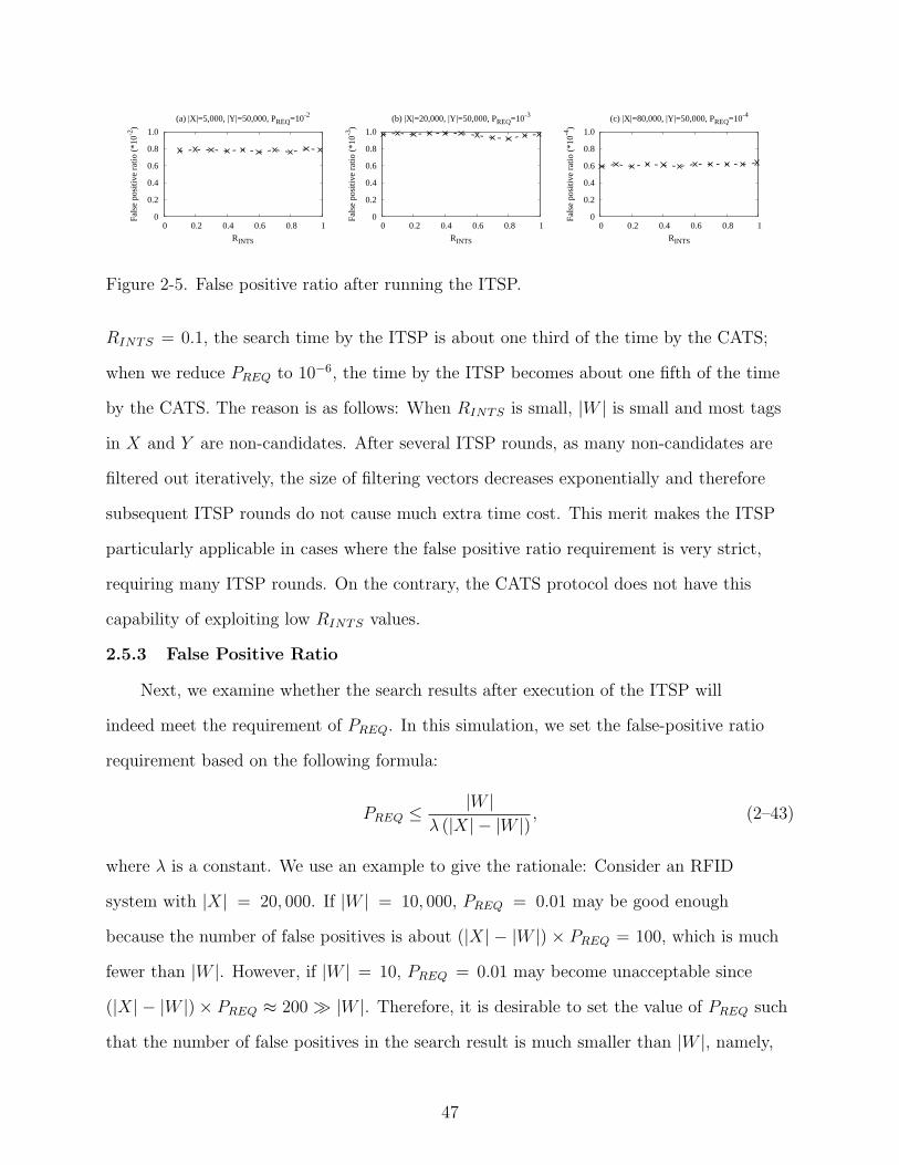
0
0.2
0.4
0.6
0.8
1.0
0 0.2 0.4 0.6 0.8 1
Fals
e po
sitiv
e ra
tio (
*10-2
)
RINTS
(a) |X|=5,000, |Y|=50,000, PREQ=10-2
0
0.2
0.4
0.6
0.8
1.0
0 0.2 0.4 0.6 0.8 1
Fals
e po
sitiv
e ra
tio (
*10-3
)
RINTS
(b) |X|=20,000, |Y|=50,000, PREQ=10-3
0
0.2
0.4
0.6
0.8
1.0
0 0.2 0.4 0.6 0.8 1
Fals
e po
sitiv
e ra
tio (
*10-4
)
RINTS
(c) |X|=80,000, |Y|=50,000, PREQ=10-4
Figure 2-5. False positive ratio after running the ITSP.
RINTS = 0.1, the search time by the ITSP is about one third of the time by the CATS;
when we reduce PREQ to 10−6, the time by the ITSP becomes about one fifth of the time
by the CATS. The reason is as follows: When RINTS is small, |W | is small and most tags
in X and Y are non-candidates. After several ITSP rounds, as many non-candidates are
filtered out iteratively, the size of filtering vectors decreases exponentially and therefore
subsequent ITSP rounds do not cause much extra time cost. This merit makes the ITSP
particularly applicable in cases where the false positive ratio requirement is very strict,
requiring many ITSP rounds. On the contrary, the CATS protocol does not have this
capability of exploiting low RINTS values.
2.5.3 False Positive Ratio
Next, we examine whether the search results after execution of the ITSP will
indeed meet the requirement of PREQ. In this simulation, we set the false-positive ratio
requirement based on the following formula:
PREQ ≤ |W |λ (|X| − |W |)
, (2–43)
where λ is a constant. We use an example to give the rationale: Consider an RFID
system with |X| = 20, 000. If |W | = 10, 000, PREQ = 0.01 may be good enough
because the number of false positives is about (|X| − |W |) × PREQ = 100, which is much
fewer than |W |. However, if |W | = 10, PREQ = 0.01 may become unacceptable since
(|X| − |W |)× PREQ ≈ 200 ≫ |W |. Therefore, it is desirable to set the value of PREQ such
that the number of false positives in the search result is much smaller than |W |, namely,
47

(|X| − |W |) × PREQ ≤ 1λ|W |. Let λ = 10 and we test the ITSP under three different
parameter settings:
(a) |X| = 5, 000, |Y | = 50, 000, and RINTS varies from 0.1 to 0.9, i.e., |W | varies from 500to 4,500. PREQ ≤ 500
10×(5,000−500)≈ 0.01111. We set PREQ = 10−2.
(b) |X| = 20, 000, |Y | = 50, 000, and RINTS varies from 0.01 to 0.9, i.e., |W | varies from200 to 18,000. PREQ ≤ 200
10×(20,000−200)≈ 0.00101. We set PREQ = 10−3.
(c) |X| = 80, 000, |Y | = 50, 000, and RINTS varies from 0.01 to 0.9, i.e., |W | varies from500 to 45,000. PREQ ≤ 500
10×(80,000−500)≈ 0.00063. We set PREQ = 10−4.
For each parameter setting, we repeat the simulation 500 times to obtain the average false
positive ratio.
Fig. 2-5 shows the simulation results. In (a), (b), and (c), we can see that the average
PFP is always smaller than the corresponding PREQ. Hence, the search results using the
ITSP meet the prescribed requirement of false positive ratio in the average sense.
If we look into the details of individual simulations, we find that a small fraction of
simulation runs have PFP beyond PREQ. For example, Fig. (2-6) depicts the results of 500
runs with |X| = 5, 000, |Y | = 50, 000, |W | = 500 and PREQ = 10−2. There are about 5%
runs having PFP > PREQ, but that does not come as a surprise because the false positive
ratio in the context of filtering vectors (ITSP) or Bloom filters (CATS) is defined in a
probability way: The probability for each tag in X − W to be misclassified as one in W
is no greater than PREQ. This probabilistic definition enforces a requirement PREQ in an
average sense, but not absolutely for each individual run.
2.5.4 Performance Evaluation under Channel Error
2.5.4.1 Performance of ITSP-rem and ITSP-bem
We evaluate the performance of ITSP-rem and ITSP-bem. To simulate the error
rate PERR in ITSP-rem, we employ a pseudo-random number generator, which generates
random real numbers uniformly in the range [0, 1]. If a bit in the filtering vector is ‘0’
and the generated random number is in [0, PERR], that bit is flipped to ‘1’. PS can
be simulated in a similar way. As for the burst error in ITSP-bem, we first calculate
48

00.20.40.60.81.01.2
0 50 100 150 200 250 300 350 400 450 500fals
e po
sitiv
e ra
tio (
*10-2
) Parameter setting: |X|=5000, |Y|=50000, RINTS=0.1, PREQ=0.01
Figure 2-6. False positive ratio by the ITSP of 500 runs.
the values of Pl(w) with different w for a given l. Then each w is assigned with a
non-overlapping range in [0, 1], whose length is equal to the value of Pl(w). For each
interval, we generate a random number and check which range the number locates, thereby
determining the number of errors in that interval.
We set PREQ = 0.001, PS = 0.01, and RINTS = 0.1, 0.5, 0.9, respectively. The values
of |X| and |Y | are the same as those in Tables 2-4 and 2-5. ls is set to 80 bits and a 16-bit
CRC is appended to each segment on forward link for integrity check. For ITSP-rem, we
consider two cases with PERR = 5% and 10% respectively. For ITSP-bem, the prescribed
parameters are set to be: η = 0.135, τ = 7.10 with each interval to be 96 bits [62].
Tables 2-6 ∼ 2-11 show the number of ts slots needed under each parameter setting.
The second column presents the results of ITSP when the channel is perfectly reliable.
The third and fourth columns present the results of ITSP-rem with an error rate of 5%
or 10%. The fifth column presents the results of ITSP-bem. It is not surprising that the
search process under noisy channel generally takes more time due to the use of CRC and
the higher false positive-probability of filtering vectors, and the execution time of the
ITSP-rem is usually longer in a channel with a higher error rate. An important positive
observation is that the performance of the proposed protocol gracefully degrades in all
simulations. The increase in execution time for both ITSP-rem and ITSP-bem is modest,
compared to ITSP with a perfect channel. For example, even when the error rate is 10%,
49

Table 2-6. Performance comparison. |Y |=50,000, RINTS=0.1, PREQ = 0.001.
|X| ITSP I TSP-rem ITSP-bemPERR = 5% PERR = 10%
5,000 61,463 74,288 75,812 72,14410,000 108,017 129,995 133,022 125,77920,000 185,204 241,026 247,824 238,96240,000 304,767 361,242 398,198 358,36180,000 414,686 441,365 458,433 437,256160,000 472,677 504,565 545,338 499,058320,000 529,835 567,403 630,174 560,456640,000 573,270 626,379 690,400 618,913
Table 2-7. Performance comparison. |Y |=50,000, RINTS=0.5, PREQ = 0.001.
|X| ITSP I TSP-rem ITSP-bemPERR = 5% PERR = 10%
5,000 105,828 160,481 166,469 153,83810,000 206,709 211,513 221,771 210,80520,000 335,426 371,974 391,983 370,55740,000 512,156 577,305 617,196 577,30580,000 656,426 735,592 789,874 735,592160,000 721,347 793,482 865,617 793,482320,000 721,347 793,482 865,617 793,482640,000 721,347 793,482 865,617 793,482
the execution time of ITSP-rem is about 10% ∼ 30% higher than that of ITSP. This
modest increase demonstrates the practicality of our protocol under noisy channel.
Table 2-8. Performance comparison. |Y |=50,000, RINTS=0.9, PREQ = 0.001.
|X| ITSP I TSP-rem ITSP-bemPERR = 5% PERR = 10%
5,000 124,553 156,041 163,718 155,97210,000 231,236 275,394 290,493 275,25620,000 403,954 454,929 486,150 454,92940,000 678,066 752,753 814,890 752,75380,000 721,347 793,482 865,617 793,482160,000 721,347 793,482 865,617 793,482320,000 721,347 793,482 865,617 793,482640,000 721,347 793,482 865,617 793,482
50

Table 2-9. Performance comparison. |X|=10,000, RINTS=0.1, PREQ = 0.001.
|Y | ITSP I TSP-rem ITSP-bemPERR = 5% PERR = 10%
1,250 13,047 14,868 15,898 14,1742,500 24,289 26,626 28,617 25,2835,000 42,835 46,994 50,863 44,39310,000 73,909 76,807 84,135 75,98320,000 95,833 103,255 106,693 102,12140,000 111,904 133,043 137,348 130,382
Table 2-10. Performance comparison. |X|=10,000, RINTS=0.5, PREQ = 0.001.
|Y | ITSP I TSP-rem ITSP-bemPERR = 5% PERR = 10%
1,250 18,033 19,837 21,640 19,8372,500 36,067 39,674 43,280 39,6745,000 68,528 77,021 82,448 77,02110,000 119,022 134,208 143,261 134,20820,000 169,065 202,891 212,105 202,46740,000 174,926 214,563 224,227 213,970
Table 2-11. Performance comparison. |X|=10,000, RINTS=0.9, PREQ = 0.001.
|Y | ITSP I TSP-rem ITSP-bemPERR = 5% PERR = 10%
1,250 18,033 19,837 21,640 19,8372,500 36,067 39,674 43,280 39,6745,000 72,134 79,348 86,561 79,34810,000 144,269 158,696 173,123 158,69620,000 192,960 217,245 232,272 217,24540,000 232,904 261,277 277,300 261,173
0
0.5
1.0
1.5
2.0
2.5
3.0
0 0.2 0.4 0.6 0.8 1
Fals
e po
sitiv
e ra
tio (
*10-2
)
RINTS
(a) |X|=5,000, |Y|=50,000, PREQ=10-2
ITSP-rem(5%)ITSP-rem(10%)
ITSP-bem
0
0.5
1.0
1.5
2.0
2.5
3.0
0 0.2 0.4 0.6 0.8 1
Fals
e po
sitiv
e ra
tio (
*10-3
)
RINTS
(b) |X|=20,000, |Y|=50,000, PREQ=10-3
ITSP-rem(5%)ITSP-rem(10%)
ITSP-bem
0
0.2
0.4
0.6
0.8
1.0
0 0.2 0.4 0.6 0.8 1
Fals
e po
sitiv
e ra
tio (
*10-4
)
RINTS
(c) |X|=80,000, |Y|=50,000, PREQ=10-4
ITSP-rem(5%)ITSP-rem(10%)
ITSP-bem
Figure 2-7. False positive ratio after running ITSP-rem, ITSP-bem and CATS.
51

2.5.4.2 False positive ratio of ITSP-rem and ITSP-bem
We use the same parameter settings in Section 2.5.3 to examine the accuracy of
search results by ITSP-rem and ITSP-bem. Meanwhile, for ITSP-rem, we set PERR = 5%
or 10%. For ITSP-bem, the required input parameter setting is η = 0.135 and τ = 7.10,
with each 96-bit interval. Simulation results are delineated in Fig. 2-7, where the error
rate is given between the parentheses after ITSP-bem. Clearly, the false positive ratio in
the search results after executing ITSP-rem or ITSP-bem is always within the bound of
PREQ. These results confirm that the false-positive ratio requirement is met under noisy
channel.
2.5.4.3 Signal loss due to fading channel
We consider the scenario of a time-varying channel in which it may happen that a
signal from a tag is not received by the reader in a deep fading slot. Although we consider
this condition is relatively rare in a RFID system that is configured to work stably, we
acknowledge in Section 2.4.2 that ITSP (or CATS) is not robust against this type of error.
However, the problem can be alleviated by the tags transmitting each filtering vector
twice. Figure 2-8 shows the simulation results under parameters |X| = 10000, |Y | = 5000,
|W | = 500, and PREQ = 0.01. The horizontal axis shows the error rate, which is defined
as the fraction of slots in deep fading, causing complete signal loss. ITSP-2 denotes
the approach of transmitting each filtering vector from tags to the reader twice. When
a wanted tag in W is not identified, we call it a false negative. The simulation results
show that ITSP incurs significant false negatives when the error rate becomes large. For
example, when the error rate is 2%, the average number of false negatives is 90.7. ITSP-2
works very well in reducing this number. When the error rate is 2%, its number of false
negatives is just 1.95.
2.6 Summary
This chapter studies the tag search problem in large-scale RFID systems. To improve
time efficiency and eliminate the limitation of prior solutions, we propose an iterative tag
52

0
100
200
300
400
500
0.01 0.02 0.03 0.04 0.05
num
ber
of f
alse
neg
ativ
es
error ratio
ITSPITSP-2
Figure 2-8. False negatives due to signal loss in time-varying channel.
search protocol (ITSP) based on a new technique that iteratively applies filtering vectors.
Moreover, we extend the ITSP to work under noisy channel. The main contributions of
our work are summarized as follows: (1) The iterative method of ITSP based on filtering
vectors is very effective in reducing the amount of information to be exchanged between
tags and the reader, and consequently saves time in the search process; (2) the ITSP
performs much better than the existing solutions; (3) the ITSP works well under all
system conditions, particularly in situations of |X| ≫ |Y | when CATS works poorly; (4)
the ITSP is improved to work effectively under noisy channel.
53

CHAPTER 3A LIGHTWEIGHT CIPHER FOR RFID SYSTEMS
3.1 Security Model
3.1.1 System Model
An RFID system consists of a large number of tags, one or multiple readers, a
backend server, and the communication channels between them. There are three types
of RFID tags: active tag, passive tag and semi-active tag. In this chapter, we focus on
the low-cost passive tags, which are powered by radio energy emitted from the readers.
The computation and storage capabilities of each tag are very limited. The backend
server, which takes charge of data storage, lookup and high-performance computations,
is connected with the readers via high speed wired or wireless links. A reader must be
authorized by the backend server before accessing confidential information, such as tag
IDs and secret keys. Since the backend server and the readers have abundant resources to
implement effective cryptographic primitives, they have no difficulty in establishing secure
connections. Therefore, an authorized reader and the backend server can be considered
as an integrated entity, still called an authorized reader. An unauthorized reader has no
right to access the backend server, but it can eavesdrop on the wireless channels between
the readers and tags. Note that in the following discussion, a reader without further
annotation is an authorized one by default.
However, none of the above ciphers goes beyond the traditional paradigm for
cryptography design: The two communicating parties are thought to be equipotent
entities with comparable capabilities, and they should execute the protocols independently.
This is true when communications happen between full-fledged computers. When it comes
to RFID systems, however, a reader is much more powerful than a tag. If we stuck with
the traditional paradigm when designing a new cipher, the tag would have to operate the
same cryptographic functions as those implemented on the reader, which poses a heavy
workload on the tag.
54

3.1.2 Adversary Model
An adversary will exploit the weaknesses of the RFID system to achieve malicious
objectives. In [64], the authors classify adversaries based on their objectives, level of
interference, presence, and available resources. In our model, we assume the major purpose
of the potential adversary is to intercept confidential information exchanged between the
readers and the tags. The adversary is capable of manipulating a few unauthorized readers
to eavesdrop on both the forward channel (reader to tag commands) and the backward
channel (tag to reader responses). Moreover, the adversary possesses sufficient storage
resources to record all messages it overhears for further analysis. Finally, for the sake of
not being detected, the adversary will never carry out disruptive attacks that may expose
its presence.
3.2 Related Work
Recently, some work focused on studying lightweight ciphers, and a number
of cryptographic algorithms have been proposed. Since asymmetric (public-key)
cryptography usually demands more computation resources than symmetric (secret-key)
cryptography, most lightweight ciphers are developed in the scope of the latter. In [65],
the authors classify existing lightweight ciphers into three categories: Some researchers
tried to optimize and compact standardized block ciphers, like AES [66–68] and IDEA
[69], thereby reducing their hardware requirements and making them suitable for
resource-constrained devices. Those algorithms fall into the first category. The algorithms
in the second category are devised by slightly revising classical block ciphers, so they
can be applied to lightweight applications. For example, DESL and DESXL [70] are
lightweight variants of DES. The third category includes a set of new algorithms that are
particularly designed for low-cost devices such as RFID tags and wireless sensors. Among
them are lightweight block ciphers, such as PRESENT [71], HIGH [72] and mCrypton [73],
and compact stream ciphers, such as Grain, MICKEY and Trivium [74], which are the
55

achievements from the eSTREAM project, while Hummingbird [65] is a hybrid of block
cipher and stream cipher.
However, none of the above ciphers goes beyond the traditional paradigm for
cryptography design: The two communicating parties are thought to be equipotent
entities with comparable capabilities, and they should execute the protocols independently.
This is true when communications happen between full-fledged computers. When it comes
to RFID systems, however, a reader is much more powerful than a tag. If we stuck with
the traditional paradigm when designing a new cipher, the tag would have to operate the
same cryptographic functions as those implemented on the reader, which poses a heavy
workload on the tag.
3.3 Cipher design
3.3.1 Motivation
A stream cipher generates a pseudorandom bit stream, called keystream, and uses
it to encrypt the plaintext with a simple XOR operation. Compared with block ciphers,
stream ciphers generally have a higher execution speed and a lower hardware complexity,
which makes them better candidates for low-cost RFID tags. Since typical stream ciphers
belong to symmetric ciphers, it is imperative that every RFID tag must independently
produce the keystream if we want to apply such ciphers to RFID systems. However,
implementation of common stream ciphers, such as RC4, incurs significant hardware cost.
For example, RC4 built by [75] takes 13K GE (logic gate equivalence). Alternatively,
we may leverage cryptographic hash functions to generate pseudorandom numbers
and transform them into a keystream. A common hash function, such as MD4, MD5,
and SHA-1, usually requires more than 7K logic gates [33]. In contrast, a low-cost
RFID tag is only integrated with 7K-15K logic gates, of which 2K-5K are used for
security purposes[64]. This bottleneck makes it impractical to implement complicated
cryptographic functions on low-cost tags. Our goal is to design a new stream cipher that is
more hardware-efficient for tags.
56

One interesting idea is as follows: If we handed the burdensome task of generating
a keystream over to a reader and let the reader secretly inform the tags the generated
keystream on the fly, the functions implemented on the tags could be much simplified. For
example, suppose each RFID tag had an unlimited memory, and was pre-configured with
infinite number of different ⟨index, key⟩ pairs, which were shared by the reader. When
the reader communicates with a tag, it generates random indexes one by one to decide
which keys to use. Meanwhile, those indexes are sent to the tag in sequence notifying it
of the currently selected keys. Once a key is used, it will be deleted by the reader and the
tag to avoid duplicate use. The reader and the tag can generate the same keystream by
concatenating the chosen keys in order. More importantly, it is an easy task for the tag to
construct the keystream according to the received indexes.
Unfortunately, far from infinity, the memory size of a passive tag is actually very
limited, and even a small number of keys can occupy its whole memory. According to
the EPC C1G2 standard[2], the memory of a tag logically comprises four distinct banks:
reserved memory, EPC memory, TID memory, and user memory. User memory can be
used for user-specific data storage, such as security keys. A passive UHF tag usually owns
a 512-bit user memory. Even some high-end tags only have a memory capacity of up to
32KB [76–78], and the prices of such tags are much higher. For example, the x Sky-ID tag
[76] with 8KB user memory currently costs $25 each. Due to the cost reason, we assume
that the available user memory for storing keys, denoted as M bits, is no larger than 1Kb
when we design our cipher.
We call the small number of keys accommodated by each tag base keys. Suppose the
length of each base key is L bits, and the number of base keys in each tag is N . Clearly,
the condition N × L ≤ M must hold. In this case, those base keys must be reused and
updated to produce a massive number of so-called derived keys, which are used to form
a keystream for encryption. Our basic idea is that the reader makes use of its powerful
computation capability to generate derived keys with good randomness, and meanwhile it
57

encodes the information about how each derived key is generated into messages sent to the
tag. Instructed by the received messages, the tag can retrieve the same derived keys with
little effort. To assist the tag in generating derived keys one by one on the fly, the reader
divides its messages into L-bit blocks and encodes the information for producing derived
keys in the message blocks.
The length of every derived key is fixed to L bits, the same as that of the base keys.
We use K to represent the key space of all possible derived keys generated from the N
base keys, and our objective is two-fold: (1) The cardinality of K should be 2L, namely,
K contains all possible values of L bits long; (2) the probability for the appearance of any
derived key in K is approximately equivalent to 12L.
3.3.2 Design Details
We now describe our lightweight cipher Pandaka in detail, where tags only need to
perform three simple operations: bitwise XOR, one-bit left circular shift, and bit flip. To
simplify the discussion, we just consider the communications between one reader and one
tag.
3.3.2.1 Initialization
First of all, some base keys must be shared by the reader and the tag. To generate
a number N of L-bit base keys, denoted by k0, k1, ..., kN−1, respectively, the reader
employs a random number generator that produces random numbers uniformly in the
range {0, 1, ..., 2L − 1}. Those N base keys are configured into the tag’s user memory
before deployment. Also, those base keys as well as the corresponding tag ID are stored in
the backend database, so the reader can retrieve the base keys with the tag’s ID.
3.3.2.2 Derived keys generated by the reader
We design an algorithm for the reader to produce derived keys based on the base
keys. To generate a derived key k, each base key ki (0 ≤ i ≤ N − 1) is independently
selected with a probability 12. The selection process is achieved by a random bit generator
that can uniformly produce 0 and 1. Before determining whether ki is chosen or not, the
58

k1/Yes
k0/No
. . .
k
0
1
N
k
-1
1/Yes
1/Yes
k2
. . .
chosen?
chosen?
chosen?
chosen?
Figure 3-1. Generation of derived keys.
reader calls the generator to produce a random bit. The base key ki will be chosen only if
the bit is 1. We denote the set of the chosen base keys as KC. Obviously, there are 2N − 1
possible results for KC, excluding the case that KC is empty when no base key is selected.
Afterwards, the reader calculates k by applying XOR operation on all elements in KC. For
instance, if KC = {k0, k2, kN−1}, then k = k0 ⊕ k2 ⊕ kN−1. The complete process for
generating a derived key is illustrated in Fig. 3-1.
3.3.2.3 Base key update by the reader
Once a derived key is generated, the selected base keys should be updated to refresh
the key materials. This time, the reader reuses the random bit generator in 3.3.2.2 to
generate two random bits. Accordingly, four different update patterns are devised. For
every chosen base key, it first performs a one-bit left circular shift as shown in Fig.
3-2, where a one-bit left circular shift is applied on the sequence (0110 1101)2. Next, a
corresponding update pattern is adopted based on the two random bits as follows:
(1) Pattern 0: The two bits are 00. Nothing is to be done.
(2) Pattern 1: The two bits are 01. The reader flips the bits in the base key whoseposition indexes mod 3 is equal to 0.
(3) Pattern 2: The two bits are 10. The reader flips the bits in the base key whoseposition indexes mod 3 is equal to 1.
(4) Pattern 3: The two bits are 11. The reader flips the bits in the base key whoseposition indexes mod 3 is equal to 2.
After that, the update process at the reader side is finished.
59

0 1
MSB LSB
0 0
0 0 0
1 1 1 1
1 1 1 1 1
Figure 3-2. One-bit left circular shift.
3.3.2.4 Design rationale
The rationale behind our update scheme is to reduce the mutual dependence between
bits in each base key. We let L = 2λ, where λ is a constant integer, and denote the L
bit positions in the base key ki as b[i][L − 1], ..., b[i][1], b[i][0]. According to our update
scheme for base keys, those L positions can be divided into three flipping groups, such
that all bits in the same group will be flipped together if the corresponding update
pattern is chosen, while bits belonging to different groups will never be flipped together.
For example, if L = 8, the eight positions in ki are divided into three flipping groups:
{b[i][0], b[i][3], b[i][6]}, {b[i][1], b[i][4], b[i][7]} and {b[i][2], b[i][5]}.
Consider two arbitrary bits in ki, denoted by X and Y , which are treated as discrete
random variables ∈ {0, 1}. Suppose X and Y initially locate at b[i][p] and b[i][q] (0 ≤
p < q ≤ L − 1), respectively. Based on their relation when being updated, they are
classified into two categories: (1) If 3 - (q − p) and 3 - (L + p − q), X and Y will never
move to two positions that belong to the same flipping group. In other words, there is no
chance for them to be flipped together. (2) If 3 | (q − p) or 3 | (L + p − q), X and Y may
appear at two positions that are in the same flipping group, thereby possibly being flipped
together (Note that by no means will both 3 | (q − p) and 3 | (L + p − q) hold because
3 - L). More specifically, within a period of L updates such that X and Y return to their
original positions, if 3 | (q − p), X and Y are in the same flipping group for (L − (q − p))
times, and if 3 | (L + p − q), X and Y may be flipped together for (q − p) times. For
example, we let L = 8. If X is at b[i][0] and Y is at b[i][4] at the beginning, they belong
60

MSB LSB
XY
MSB LSB
X Y
Figure 3-3. Illustration of two bits that initially belong to the same flipping group movingto different flipping groups.
to the first category. In contrast, if initially X is at b[i][0] and Y is at b[i][3], they belong
to the second category. Their initial positions are in the same flipping group, but after
five updates, they respectively move to b[i][5] and b[i][0], which are no longer in the same
flipping group, just as illustrated in Fig. 3-3, where positions of the same flipping group
are marked with the same color.
In conclusion, there is always a chance for any two bits X and Y in a base key to
appear at positions in different flipping groups regardless of their initial positions, and
then they can be flipped asynchronously, which reduces their mutual dependence.
3.3.2.5 Indicator for the tag
Now that it is clear how the reader generates derived keys and updates the base keys,
we proceed to show how those two processes can be repeated by the tag in a simpler way.
To establish secure communication channels, the reader and the tag should always share
the same base keys and generate same derived keys. Hence, each time the reader has to
somehow inform the tag its choices of base keys and update pattern, thus instructing the
tag to generate the same derived key and update the base keys following the same pattern.
To do so, the reader encodes all necessary information into a bit vector, which is called an
indicator, and sends that indicator to the tag. Let us take a look at the structure of an
indicator as illustrated in Fig. 3-4: It is a (N + 2)-bit vector, where the low-order N bits
represent the reader’s choices of base keys. If the ith bit in the indicator is ‘1’, it means
the ith base key is selected; otherwise, the ith base key is not chosen by the reader. The
remaining two high-order bits in an indicator manifest the update pattern for those chosen
base keys.
61

10 01 1 ...0
MSB LSB
update bit selectorN-pattern
Figure 3-4. A (N + 2)-bit indicator.
With the help of an indicator, the tag knows exactly which base keys should be used
to calculate the derived key and how to update the selected base keys. Note that there is
no need for the tag to implement the same random number generators as the reader does,
which simplifies the tag’s function.
3.3.2.6 Formats of message blocks
The length of a message block is fixed to L bits, and it is bitwise XORed with a
derived key for encryption. To avoid the leakage of information in an indicator, it is
encrypted as part of a message block. This brings about a problem that no existing
derived key can be used to encrypt the first indicator. To address the problem, the reader
generates another L-bit random number when initializing the tag, and that random
number is stored in both the reader and the tag, serving as the first (pre-stored) derived
key. One or more indicators for subsequent derived keys can be piggybacked by current
message block, which is encrypted before transmission.
To accomplish the mutual communication between the reader and the tag, we design
three different formats of message blocks, which are depicted in Fig. 3-5. The format 1,
denoted by F1, shows how the reader organizes its message to be sent. A L-bit F1 message
block is composed by two parts: the high-order (L−N−2) bits are data to be transmitted,
and the low-order (N + 2) bits represent an indicator. The format 2, denoted by F2, is
utilized by the reader to assist the tag in generating derived keys when the tag intends
to transmit some data to the reader. Each F2 message consists of ⌊ LN+2
⌋ indicators, while
the remaining (L − ⌊ LN+2
⌋ × (N + 2)) high-order bits are padded with 0s. The format 3,
62

...
-bit indicator-bit data
01 ...
L-N-2( ) N+2
Type 1
( )
MSB LSB
1 10 0 00
... ... ... ...
padding indicator
1 1 10 0 0
Type 2MSB LSB
indicator
...
-bit data
...
L
0 0 0 0 01 1 1
Type 3MSB LSB
Figure 3-5. Different formats of message blocks.
...
-bit encrypted message
...
L 16-bit CRC
1 1 10 0 0 0 0
MSB LSB
Figure 3-6. Overall format of transmitted message blocks.
denoted by F3, is employed by the tag to send its data to the reader, where all bits are
used for encoding the data to be transmitted.
No matter which of the three formats is used, a CRC code is calculated for that
block before encryption. A C1G2 RFID tag supports two CRC types: 16-bit CRC
and 5-bit CRC[2]. In this chapter, we adopt the 16-bit CRC code for the purpose of
integrity verification of message blocks. For each CRC code, it is transmitted along with
its corresponding ciphertext block. Fig. 3-6 shows the overall format of a transmitted
message block. After receiving a block, the reader or the tag first strips the L-bit
encrypted message to decrypt it, and then calculates the CRC code of the decrypted
block, which is compared with the attached CRC code. If the verification of the CRC code
fails, the reader or the tag sends a request for retransmission of that block.
3.3.3 Two-Phase Communications
Communications between the reader and tag are always initialized by the reader.
Each session consists of two phases: In phase one, the reader transmits an encrypted
63

message to the tag, and during phase two, the tag sends its encrypted message with the
aid of the reader. More generally, phase one or phase two may be skipped if there is only a
one-way message to be transmitted. Before exchanging the messages, the reader first sends
a query to the tag, and the tag responds with its ID (Note that privacy of tag ID is not
our concern in this chapter). Using this received ID, the reader can retrieve the set of base
keys and the pre-stored derived key (or the derived key left from last session) from the
backend server.
3.3.3.1 Phase one
In phase one, the reader encrypts and sends message blocks in form of F1 to the tag
continuously. The reader segments its message into (L − N − 2)-bit blocks. For each
(L−N − 2)-bit data block, the reader combines it with a randomly generated (N + 2)-bit
indicator. The derived key for encrypting the first block is the pre-stored random number
or left from last session. The message blocks are XORed with the corresponding derived
keys for encryption, and then consecutively sent by the reader to the tag in order. Once
receiving an encrypted block, the tag is capable of decrypting it using the corresponding
derived key. The tag extracts and stores the high-order (L − N − 2)-bit data from the
decrypted block. Meanwhile, the tag calculates the next derived key and updates the
chosen base keys guided by the indicator. Note that the indicator can be discarded once it
is used. When the transmission is done, the reader informs the tag that phase one ends, so
the tag can switch to phase two.
3.3.3.2 Phase two
Phase two may consist of multiple rounds, where message blocks are exchanged
bidirectionally. In each round, the reader first randomly creates ⌊ LN+2
⌋ indicators, which
are concatenated into a F2 message block. Among those ⌊ LN+2
⌋ indicators, the first
(⌊ LN+2
⌋ − 1) ones instruct the tag to generate derived keys that will be used for encrypting
its own message, while the last one specifies the derived key that the reader will use
to encrypt the next F2 block. Afterwards, the reader encrypts the F2 block with a
64

0
0.75
0.251
0.75
0.25
Figure 3-7. State transitions of one bit.
derived key. The first derived key used by the reader in phase two is the last key left
from phase one. The tag divides its message to be transmitted into blocks of format F3.
When receiving a message block from the reader, the tag decrypts it, thereby obtaining
the ⌊ LN+2
⌋ indicators. The tag then takes one indicator at a time (from low-order to
high-order) to compute a derived key, which is XORed with a F3 block for encryption.
The encrypted message block is sent to the reader. Totally, (⌊ LN+2
⌋ − 1) blocks of format
F3 can be transmitted by the tag in one round. The reader knows exactly which derived
key is used by the tag to encrypt each block, and therefore can decrypt it correctly to
obtain the original message. This process continues round by round until the tag finishes
transmitting its message. One may notice that at the end of phase two, at least one
indicator is not used, namely, the last indicator in the final F2 block sent by the reader,
and it is shared by the reader and the tag. This guarantees that the reader can initiate
another session anytime using the derived key generated with that indicator.
3.3.4 Randomness Analysis
3.3.4.1 Randomness
Randomness is a probabilistic property that is the most important metric for
assessing a random number generator or a stream cipher. For our protocol, it is of
great importance that the generated derived keys are random and unpredictable. Before
we lucubrate the randomness of the derived keys, we first study the randomness of a base
key ki during its consecutive updates.
First, we consider one arbitrary bit in ki, whose value is designated as random
variable X ∈ {0, 1}. Suppose X is currently located at position b[i][j] (0 ≤ j ≤
L − 1). When ki is updated, X is shifted and then flipped with a probability of 0.25
65

00 01
0.5 0.5
0.25
0.25
10
0.5
11
0.5
0.25 0.25
0.25
0.25
0.25 0.25
00 11
0.75 0.75
0.25
0.25
01
0.75
10
0.75
0.25
0.25
Figure 3-8. State transitions of two bits.
regardless of its new position. Fig. 3-7 shows the probabilities of state transitions of
X. Correspondingly, the transition matrix for X during each update is given by P1 = 0.75 0.25
0.25 0.75
. Using singular value decomposition (SVD), P1 =
√22
√22
√22
−√22
×
1 0
0 12
×
√22
√22
√22
−√22
. Since the choice of an update pattern is independent with each
other, after α updates, the transition matrix for X is P1α =
√22
√22
√22
−√22
×
1 0
0 12
α
×
√22
√22
√22
−√22
=
12+ 1
2
α+1 12− 1
2
α+1
12− 1
2
α+1 12+ 1
2
α+1
, which converges to
0.5 0.5
0.5 0.5
quickly as α
increases. We take α = 8 as an example, P18 =
0.502 0.498
0.498 0.502
. Therefore, whatever
the initial value of X is, it turns to be 0 or 1 with about equal probabilities after several
updates. Based on the above analysis, we conclude that the bit at any position in ki is
equally likely to be 0 or 1 in long term.
Now let us investigate two arbitrary bits in an arbitrary base key ki, denoted by
X and Y . Suppose X and Y are initially located at b[i][p] and b[i][q], respectively.
Recall from Section 3.3.2.4 that the relation between X and Y can be classified into
two categories based on their original positions in ki. For the first category, X and Y
are updated independently. Therefore, the values at b[i][p] and b[i][q] are independent. If
66

X and Y belong to the second category, the mutual influence makes the situation more
complicated. The left half of Fig. 3-8 shows state transitions of XY when they are flipped
asynchronously, while the right half shows state transitions when they are flipped together.
The corresponding transition matrixes for left half and right half of Fig. 3-8 are
P2 =
0.5 0.25 0.25 0
0.25 0.5 0 0.25
0.25 0 0.5 0.25
0 0.25 0.25 0.5
,
P3 =
0.5 0 0 0.5
0 0.5 0.5 0
0 0.5 0.5 0
0.5 0 0 0.5
.
Assume that within L updates, X and Y move to positions belonging to different flipping
groups for β times, and positions in the same flipping group for γ times, subjecting to
1 ≤ β < L, 1 ≤ γ < L, and β + γ = L. We observe that
P2β × P3
γ =
0.25 0.25 0.25 0.25
0.25 0.25 0.25 0.25
0.25 0.25 0.25 0.25
0.25 0.25 0.25 0.25
for arbitrary combination of β and γ. Hence, for any two bits in ki, regardless of their
initial values, they will have the same probability of 0.25 to become 00, 01, 10, and 11
when they are shifted back to their original positions after L updates. In other others, the
bits in ki become pairwise independent.
With the above insight, we go further to study the randomness of the derived keys.
Let us consider the jth bit in every base key. Suppose the number of 0s in those N bits is
n0[j], and the number of 1s is n1[j], where 0 ≤ j ≤ L − 1, and n0[j] + n1[j] = N . We
67

have proved that any bit in a base key is 0 or 1 with the same probability. Meanwhile,
the values of the jth bits in different base keys are independent. Thus, we have n0[j] ∼
B(N, 0.5), and P (n0[j] = t) =(Nt
)×(12
)N. We designate the jth bit in a derived key k as
k[j]. For the value of k[j], we should consider two possible cases: (1) n0[j] = N , namely,
there is no 1 in those N bits. In this case, k[j] is definitely 0; (2) If 0 ≤ n0[j] < N , then
k[j] can be 0 or 1. In the second case, if k[j] = 0, it implies an even number of base keys
whose jth bit is 1 are chosen, and that probability is:
P (k[j] = 0 | 0 ≤ n0[j] < N)
=
2n0[j] ×⌈n1[j]
2⌉∑
t=0
(n1[j]2t
)− 1
2N − 1
=2n0[j] × 2n1[j]−1 − 1
2N − 1
=2N−1 − 1
2N − 1,
(3–1)
which is a constant if N is fixed. Thus, we can obtain the probability for k[j] = 0 is:
P (k[j] = 0) =P (n0[j] = N)× P (k[j] = 0 |n0[j] = N)
+P (0 ≤ n0[j] < N)× P (k[j] = 0 | 0 ≤ n0[j] < N)
=1
2N× 1 + (1− 1
2N)× 2N−1 − 1
2N − 1
=1
2.
(3–2)
Therefore, P (k[j] = 1) = P (k[j] = 0) = 12, which means any bit in the derived key is
uniformly distributed over {0, 1}. Moreover, k[j] is determined only by the jth bits of the
base keys, and we have proved bits in every base key are pairwise independent, so bits in k
are also pairwise independent.
3.3.4.2 Gap length
Another metric for evaluating the performance of a random number generator is
the gaps occurring between the same digits in the series [79]. This metric can also be
68

extended to assess our algorithm for producing derived keys. Gap length, denoted by Lg,
is defined as the number of derived keys before the first recurrence of a given derived key.
For example, for a derived key whose value is 0, Lg is 3 in the derived-key sequence 0, 1, 2,
3, 0, and Lg is 4 in the derived-key sequence 0, 1, 2, 3, 3, 0. For a L-bit derived key, if it is
produced uniformly, the expectation of Lg is
E(Lg) =∞∑j=0
j × Prob(Lg = j)
=∞∑j=0
j ×(2L − 1
)j(2L)j+1
=1
2L×
∞∑j=1
j ×(1− 1
2L
)j
=1
2L×
1− 12L(
1−(1− 1
2L
))2= 2L − 1.
(3–3)
It means that before a derived key reappears it is expected that all (or most) other keys
will appear. In Section 3.4, we will conduct simulations to evaluate the randomness of the
derived keys.
3.3.5 Hardware Cost for Tag Implementation
Given the constraint that only 2K-5K GEs in low-cost tags can be used for security
functions, we estimate the hardware requirement of Pandaka to evaluate its hardware
efficiency. The number of GEs required by each cryptographic component is not a
constant and varies with actual implementation. We use the same parameters for cost
estimations as in [64], which are outlined in Table 3-1. A shift register is a group of
flip-flops connected in chain, and a circular shift register can be created by connecting
the serial input and last output of a shift register [80]. Hence, the circular shift register
can be built with L × 12 GEs, where L is the length of a base key. To generate a derived
key, we need another two L-bit registers. The first register, which is initialized to all
ones, keeps the intermediate result. Each time, the tag reads one chosen base key
69

Table 3-1. Cost estimations for typical cryptographic hardware.
Functional Block Cost (GEs)2 input NAND gate 12 input XOR gate 2.52 input AND gate 2.5FF (Flip Flop) 12n-byte RAM n× 12
from memory and stores it in the second register, which is bitwise XORed with the
first register. The intermediate result is written back to the first register. Proceeding
in this way, the derived key is finally stored in the first register after all chosen base
keys are XORed with the first register. The two registers and the XOR operation need
2 × 12 × L + L × 2.5 = 26.5 × L GEs. In addition, we need N × L bits RAM to store the
base keys, which requires N × L× 1.5 GEs. As a result, the total number of GEs for a tag
to implement Pandaka is L × 12 + L × 26.5 + N × L × 1.5 = (38.5 + 1.5N) × L, which
is determined by L and N . For example, if we let L = 16 and N = 6, a tag needs about
(38.5 + 1.5× 6)× 16 = 760 GEs to implement Pandaka; if we let L = 32 and N = 6, a tag
needs about (38.5 + 1.5 × 6) × 32 = 1520 GEs to implement Pandaka. As a comparison,
we list the hardware costs of other lightweight ciphers in Table 3-2, where Pandaka(L, N)
means Pandaka with N L-bit base keys. It is not surprising that Pandaka requires much
fewer GEs than others since it only needs to perform three simple operations.
3.4 Simulations
In this section, we use simulations to examine the randomness of derived keys in
Pandaka.
3.4.1 Frequency Test
First, we examine the randomness of derived keys using frequency test. Specified in
the EPC C1G2 Standard [2], one requirement for the generation of 16-bit pseudorandom
2 This is the number of GEs required by the most lightweight implementation ofHummingbird.
70

Table 3-2. Comparison of lightweight ciphers in terms of hardware complexity.
Cipher Key bits Block bits Cost (GEs)PRESENT-80[71] 80 64 1570PRESENT-128[71] 128 64 1886AES [66] 128 128 3400HIGHT[72] 128 64 3408mCrypton[73] 96 64 2681DES[70] 56 64 2309DESL[70] 56 64 1848DESXL[70] 184 64 2168Hummingbird[81] 128 16 2159 2
Trivium[82] 80 1 2580Trivium×8[82] 80 8 2952Trivium×16[82] 80 16 3166Grain[83] 80 1 1450Grain×8[83] 80 8 2756Grain×16[83] 80 16 4248MIKEY[82] 128 1 5039Pandaka(16, 6) 96 16 760Pandaka(32, 6) 192 32 1520
numbers is that the probability of any 16-bit number RN16 with value v being drawn
from the generator shall be bounded by 0.8216
< P (RN16 = v) < 1.25216
. We extend that
requirement to the generation of derived keys with arbitrary length L-bit: The probability
of any L-bit derived key k having value v shall be bounded by 0.82L
< P (k = v) <
1.252L
. To check whether the randomness of the derived keys meets the requirement, we
generate N random base keys, and execute the derived-key generator for 2L × r times to
produce a large number of derived keys, where r is a simulation parameter. As a result,
approximately 2L × r × (1 − 12N
) derived keys are generated. The frequency of each
derived key is defined as the number of its appearances divided by the total number
of keys derived. From simulation results, we compute the standard deviation σ for the
frequencies of derived-key values. Note that the average frequency, denoted by Favg,
should be 12L. Meanwhile, we count the number of derived keys whose frequencies locate
in (0.82L, 1.25
2L), denoted by Ns, thereby calculating the satisfactory rate, which is defined as
71

Table 3-3. Statistics for Pandaka with L = 8 and Grain×8.
Pandaka Grain×8N 1 2 3 4
Favg(×10−3) 3.91 3.91 3.91 3.91 3.91σ(×10−4) 2.4 1.9 1.8 1.7 1.7
Rs 99.6% 100% 100% 100% 100%
Table 3-4. Statistics for Pandaka with L = 16 and Grain×16.
Pandaka Grain×16N 1 2 3 4
Favg(×10−5) 1.526 1.526 1.526 1.526 1.526σ(×10−7) 9.7 7.9 7.3 7.1 6.8
Rs 99.95% 100% 100% 100% 100%
Rs =Ns
2L. Constrained by the computation capability of our computer, we are not able to
run simulations with L = 32 or larger. For this reason, we set the parameters as follows:
(a) r = 500, L = 8, and N varies from 1 to 4.
(b) r = 500, L = 16, and N varies from 1 to 4.
As a comparison, we implement Grain (Grain×8 and Grain×16 as shown in Table 3-2),
one of the most lightweight existing stream ciphers.
The simulation results are shown in Fig. 3-9, Table 3-3 and Table 3-4. To make
the figures legible, we sample a fraction of 1/50 among all derived keys for displaying.
Our results show that the frequencies of derived keys in Pandaka perfectly meet the
randomness requirement, even if the number of base keys is very small. Also, we find
that the randomness of derived key becomes better when N increases. Moreover, the
randomness of keystream in Pandaka is almost as good as that of Grain when N ≥ 4,
while recalling from Table 3-2 that the hardware cost of Pandaka(16, 6) is only about one
sixth of the cost of Grain×16.
3.4.2 Gap Test
Second, we check the randomness of derived keys by gap test. We run simulations to
obtain the gap length of any first generated derived key. Under each setting of L and N ,
the test is conducted 500 times to obtain the average value of gap length, denoted by L̄g.
72

2
3
4
5
6
0 50 100 150 200 250
Freq
uenc
y (×
10-3
)
Key Value
Pandaka, L=8, N=1
2
3
4
5
6
0 50 100 150 200 250
Freq
uenc
y (×
10-3
)
Key Value
Pandaka, L=8, N=2
2
3
4
5
6
0 50 100 150 200 250
Freq
uenc
y (×
10-3
)
Key Value
Pandaka, L=8, N=3
2
3
4
5
6
0 50 100 150 200 250Fr
eque
ncy
(× 1
0-3)
Key Value
Pandaka, L=8, N=4
0
1
2
3
0 20000 40000 60000
Freq
uenc
y (×
10-5
)
Key Value
Pandaka, L=16, N=1
0
1
2
3
0 20000 40000 60000
Freq
uenc
y (×
10-5
)
Key Value
Pandaka, L=16, N=2
0
1
2
3
0 20000 40000 60000
Freq
uenc
y (×
10-5
)
Key Value
Pandaka, L=16, N=3
0
1
2
3
0 20000 40000 60000
Freq
uenc
y (×
10-5
)
Key Value
Pandaka, L=16, N=4
2
3
4
5
6
0 50 100 150 200 250
Freq
uenc
y (×
10-3
)
Key Value
Grain×8
0
1
2
3
0 20000 40000 60000
Freq
uenc
y (×
10-5
)
Key Value
Grain×16
Figure 3-9. Frequency test for randomness.
73

1.0
1.5
2.0
2.5
3.0
1 2 3 4 5 6 7 8Ave
rage
Gap
Len
gth
(×10
2 )
Number of Base Keys
8-bit Base Keys
3.0
4.0
5.0
6.0
7.0
1 2 3 4 5 6 7 8Ave
rage
Gap
Len
gth
(×10
4 )
Number of Base Keys
16-bit Base Keys
Figure 3-10. Gap test for randomness.
The results are depicted in Fig. 3-10. According to (3–3), we know E(Lg) = 255 when
L = 8, and E(Lg) = 65535 when L = 16. We can see from Fig. 3-10 that for a given L, L̄g
rises with the increase of N at the beginning. However, the increasing rate of L̄g gradually
slows down, and finally L̄g slightly oscillates around a stable value that is very close to
E(Lg) when N ≥ 5. That is the reason why we set N = 6 for Pandaka in Section 3.3.5.
These results show that our derived key generation algorithm can achieve nice randomness
with just a few base keys.
3.5 Security Analysis of Pandaka
In this section, we consider several general attacks on Pandaka and analyze to what
extent Pandaka can resist against those attacks.
3.5.1 Ciphertext Only Attack
Suppose the adversary can only obtain some ciphertext. It has to search through
all possible base keys to decrypt the message. For each set of base keys, the adversary
tries to decrypt the ciphertext with every possible derived key, and hopes to obtain some
recognizable plaintext. However, this is not feasible as the space for base keys is as large
as 2NL (e.g. if L = 16 and N = 6, the space is 296).
3.5.2 Known Plaintext Attack
The only function of an indicator is to help the tag generate a derived key, so neither
the reader nor the tag needs to store this temporary data. Hence, we assume the only
plaintext an adversary may obtain is the data in a F1 block or a F3 block. When an
74

adversary somehow obtains a ⟨plaintext block, ciphertext block⟩ pair, it can calculate the
corresponding derived key (or part of the derived key if the plaintext is the data part of
a F1 block) by XORing them. The obtained derived keys, appearing completely random
(Section 3.4), will not provide sufficient information to break base keys, which are only
used once before being updated; without knowing the indicators, the adversary has no idea
on how the base keys are updated.
3.5.3 Time-Memory-Data Tradeoff Attack
The authors of [84] propose a new time-memory-data trade-off attack on stream
ciphers. The generic attack on a stream cipher requires about T = Ns
23 time, where
Ns represents the size of the search space. In our case, Ns = 2NL, so T = 22NL3 . If we
let N = 6 and L = 32, T = 2128, which makes the time-memory-data tradeoff attack
impracticable. Also, we should keep in mind that the base key materials are always being
updated, which makes this attack more difficult to be performed.
3.5.4 Tradeoff among Throughput, Security, and Hardware Cost
It is clear that there exists a tradeoff among throughput, security and hardware
cost in the design of Pandaka. The security of Pandaka is proportional to the number
of key bits NL, and the greater the value of NL is, the more secure Pandaka becomes.
However, when N is large, the indictors account for a large proportion of the transmitted
messages, resulting in a waste of throughput. Moreover, large NL requires more hardware
expenditure for implementing Pandaka. Hence, we should tune those two parameters
according to the different constraints and requirements in different application scenarios.
3.6 Summary
In this chapter, we propose a novel lightweight cipher Pandaka tailored to RFID
systems. Unlike classical symmetric ciphers in which two communicating parties are
burdened with equal workload, Pandaka assigns a heavy workload to the reader as it
is more powerful than the tag. The analytical and simulation results demonstrate the
effectiveness and hardware efficiency of Pandaka for low-cost tags. Complementary to the
75

traditional cryptographic design approaches, this chapter provides a new perspective for
developing symmetric cryptography in systems where significant asymmetry exists between
the communicating parties.
76

CHAPTER 4LIGHTWEIGHT ANONYMOUS RFID AUTHENTICATION
4.1 System Model and Security Model
4.1.1 System Model
Consider a hierarchical distributed RFID system as shown in Fig. 4-1. Each tag
is pre-installed with some keys for authentication. The readers are deployed at chosen
locations, responsible for authenticating tags entering their coverage areas. In addition,
the readers at each location are connected to a backend server, serving as a supplement
to provide more storage and computation resources. All backend servers are further
connected to the central server, where every tag’ keys are stored. Any authorized backend
server can fetch the tags’ keys from the central server. Since the keys of each tag are only
stored at the central server, they are synchronized from the view of different backend
servers. Moreover, the high-speed links connecting the central server, backend servers and
readers make the latency of transmitting small authentication data negligible. Therefore, a
reader, its connected backend server, and the central server can be thought as single entity,
and will be used interchangeably.
In this chapter, we focus on low-cost RFID tags, particularly passive backscatter tags
that are ubiquitously used nowadays. The simplicity of these tags contributes to their low
prices, which in turn restricts their computation, communication, and storage capabilities.
In contrast, the readers, which are not needed in a large quantity as tags do, can have
much richer resource. Moreover, the backend server can provide the readers with extra
Central server
...Backend server
Readers & Tags
... ...
Figure 4-1. A hierarchical distributed RFID system.
77

resource when necessary. The communication between a reader and a tag works in the
request-and-response mode. The reader initiates the communication by sending a request.
Upon receiving the request, the tag makes an appropriate transmission in response.
We divide the transmissions between the readers and tags into two types: (1) Invariant
transmissions contain the content that is invariant between any tag and any reader, such
as the beacon transmission from a reader which informs the incoming tag of what to do
next. (2) Variant transmissions contain the content that may vary for different tags or the
same tag at different times, such as the exchanged data for anonymous authentication.
4.1.2 Security Model
Threat model: An adversary may eavesdrop on any wireless transmissions made between
the tags and the readers. In addition, the adversary may plant unauthorized readers at
chosen locations, which communicate with passing tags and try to identify the tag carriers.
However, such unauthorized readers have no access to the backend servers or the central
server since the servers will authenticate the readers before granting access permissions.
In the sequel, a reader without further notation means an authorized one by default.
Moreover, we assume that the adversary may compromise some tags and obtain their keys,
but it cannot compromise any authorized readers.
Anonymous model: The anonymous model requires that all variant transmissions must
be indistinguishable by the adversary, meaning that (1) any variant transmission in the
protocol should not carry a fixed value that is unchanged across multiple authentications,
and (2) the transmission content should appear totally random and unrelated across
different authentications to any eavesdropper that captures the transmissions. Therefore,
no adversary will have a non-negligible advantage in successfully guessing the next variant
transmission of a tag based on the previous transmissions [85].
4.2 Related Work
Prior work on anonymous authentication can be generally classified to two categories:
non-tree-based and tree-based.
78

4.2.1 Non-Tree based Protocols
The Hash-lock [86] leverages random hash values for anonymous authentication.
After receiving an authentication request from a reader, a tag sends back (r, id ⊕ fk(r)),
where r is a random number, id is the tag’s ID, k is a pre-shared secret between the tag
and the reader, and {fn}n∈N is a pseudo-random number function ensemble. The reader
exhaustively searches its database for a tag whose ID and key can produce a match with
the received data. The hash-lock protocol has a serious efficiency problem that the reader
needs to perform O(n) hash computations on line per authentication, where n is the
number of tags in the system. Some variants [87–90] of hash-lock scheme try to improve
the search efficiency, but they have issues. The OKS protocol [87] uses hash-chain for
anonymous authentication. The OSK/AO protocol [88, 89] leverages the time-memory
tradeoff to reduce the search complexity to O(n23 ) (still too large) at the cost of O(n
23 )
units of memory. However, both OKS and OSK/AO cannot guarantee anonymity
under denial-of-service (DoS) attack [85]. The YA-TRAP protocol [90] makes use of
monotonically increasing timestamps to achieve anonymous authentication. YA-TRAP
is also susceptible to DoS attack, and a tag can only be authenticated once in each
time unit. The DoS attack in OSK/AO and YA-TRAP is in nature a desynchronization
attack, which tricks a tag into updating its keys unnecessarily and makes it fail to be
authenticated by an authorized reader later.
The LAST protocol was proposed based on a weak privacy model[91]. Key identifiers
are used to facilitate the reader to identify the tags quickly. After each authentication,
the reader uploads a new ⟨identifier, key⟩ pair to the tag. LAST only requires the reader
and tag to compute O(1) hashes per authentication, but the overhead for the reader to
search a given key identifier is not considered. Moreover, since the key identifier is only
updated after a successful authentication, the tag keeps sending the same key identifier
between two consecutive successful authentications. Therefore, LAST is not anonymous in
79

the strict sense. In addition, the process of uploading a new ⟨identifier, key⟩ pair to the
tag after each authentication incurs extra communication overhead.
4.2.2 Tree based Protocols
Tree-based protocols organize the shared keys in a balanced tree to reduce the
complexity of identifying a tag to O(log n). However, the tree-based protocols generally
require each tag to store O(log n) keys, which is O(1) for non-tree based protocols.
In Dimitriou’s protocol[92], the non-leaf nodes of the tree store auxiliary keys that
can be used to infer the path leading to leaf nodes that store the authentication keys. For
each authentication, the computation overhead for both the reader and the tag is O(log n),
and the tag needs to transit O(log n) hash values. This protocol is is vulnerable to the
compromising attack since different tags may share auxiliary keys [93, 94].
The ECNP protocol [95] leverages a cryptographic encoding technique to compress
the authentication data transmitted by tags. ECNP can reduce the computation overhead
of the reader and the transmission overhead of the tag by multifold compared with
Dimitriou’s protocol[92], but they remain O(log n) due to the use of tree structure.
Moreover, ECNP is not resistant against the compromising attack since the children of one
node in the tree share the same group keys.
The ACTION protocol [94] was designed to be resistant against the compromising
attack. It adopts a sparse tree architecture to make the keys of each tag independent
from one another. In ACTION, each tag is randomly assigned with a path key, which is
further segmented into link indices to guide the reader to walk down the tree towards the
leaf node that carries the secret key k of the tag. For each authentication, a tag needs to
compute and transmit O(log n) hashes and the reader needs to perform O(log n) hashes to
locate the shared key. The key problem of ACTION is that the size of link indices is too
small after segmentation (e.g., 4 bits), rendering them easy to guess.
80

Table 4-1. Key table for the preliminary design.
Tag Token Array Token Indext1 [tk1
1, tk21, . . . , tk
m1 ] pt1
t2 [tk12, tk
22, . . . , tk
m2 ] pt2
......
...tn [tk1
n, tk2n, . . . , tk
mn ] ptn
4.3 A Strawman Solution
Before moving to our main contributions, we propose a strawman solution for
lightweight anonymous authentication.
4.3.1 Motivation
Most prior wok, if not all, employs cryptographic hash functions to randomize
authentication data for the purpose of keeping anonymity. Implementing a typical
cryptographic hash function such as MD4, MD5, and SHA-1 requires at least 7K logic
gates [33]. However, widely-used passive tags only have 7K-15K logic gates, of which
2K-5K are reserved for security purposes[64]. The hardware constraint necessitates
a new design paradigm for lightweight anonymous authentication protocols that are
more supportive for low-cost tags. The commercial success of RFID tags lies with their
simplicity. Although there is no specification on how simple these tags should be, it is
safe to say that we will always prefer a solution that achieves the comparable goal with
less hardware requirement. On the other hand, the significant disparity between the
readers and tags points out an asymmetry design principle that we will follow: push most
complexity to the readers while leaving the tags as simple as possible.
4.3.2 A Strawman Solution
Consider an RFID system with n tags t1, t2, . . . , tn, each pre-installed with an array
of m unique random tokens, [tk1i , tk
2i , . . . , tk
mi ] (1 ≤ i ≤ n). Tag ti also has a token index
pti (initialized to 1) pointing to its first unused token. The tokens and token index of each
tag are also stored in the database of the central server, as illustrated in Table 4-1.
81

Read
er R
Tag
t
1. Authentication request
2. Token tkpt
3. Response & Token tkpt+1
Figure 4-2. Three steps of token-based mutual authentication.
In the sequel, we consider the authentication process between an arbitrary reader R
and an arbitrary tag t having a token array [tk1, tk2, . . . , tkm] and a token index pt. To
authenticate t, R sends a request to t. Upon receiving the request, t sends its first unused
token tkpt to R. After that, t increases pt by 1 to guarantee that the same token will not
be used twice. Otherwise, t will always send the same token when an unauthorized reader
requests a token, which breaks the anonymity. After receiving the token, R has to search
the token in the database since it does not know the tag’s identity. Starting from i = 1,
R checks if tkptii = tkpt one by one. If there exists an i ∈ [1, n] such that tkpti
i = tkpt,
t is successfully authenticated; otherwise, t fails the authentication. In the former case,
R sends back the token tkpti+1i to t to authenticate itself, and sets pti = pti + 2. Tag t
compares the received token with tkpt to authenticate R, and increases pt by 1 again. Fig.
4-2 shows the three steps of the mutual authentication.
In this approach, the online computation overhead of the tag is low — only one
comparison (requires far less hardware than implementing a cryptographic hash) per
authentication. The online computation complexity of the reader is O(n) since at most n
comparisons (though one comparison is much cheaper than computing one hash value) are
needed for searching the received token. The communication overhead for both the reader
and the tag is O(1).
To avoid the leakage of the tag’s identity, the tokens used for authentication should
look random. In addition, each token can be used only once. Hence, the tag must be
82

replenished with new tokens after m2mutual authentications, e.g., purchasing new tokens
from an authorized branch. Therefore, the tag should store as many tokens as possible to
reduce the inconvenience caused by token replenishment. A low-cost tag, however, only
has a tiny memory. For example, a passive UHF tag generally has a 512-bit user memory
for storing user-specific data (tokens in our case). Some high-end tags with large memory
[76, 78] are prohibitively expensive to be applied in large quantities. As an example, x
Sky-ID tags [76] with an 8KB user memory cost $25 each. We will introduce the security
issues of this design in the next section.
4.4 Dynamic Token based Authentication Protocol
In this section, we propose our first dynamic Token based Authentication Protocol
(TAP). TAP can produce tokens for anonymous authentication on demand, and therefore
does not require the tags to pre-install many tokens. However, we will show shortly that
TAP still has some problems, which will be solved by our final design in the next section.
4.4.1 Motivation
Given the memory constraint, each tag can only store a few tokens. Frequent token
replenishment brings about unacceptable inconvenience in practice. Hence, we want to
invent a way to enable dynamic token generation from the few pre-installed tokens. In
addition, the time for the reader to search a particular token is O(n) in the preliminary
design. We desire to reduce this overhead to O(1). More importantly, we hope all
advantages of the preliminary design, including no requirement of cryptographic hash
functions, low computation overhead for the tag, and low communication overhead for
both the reader and the tag, can be retained in our new design.
4.4.2 Overview
Let an arbitrary tag t in the system be pre-installed with u base tokens, denoted by
[bt1, bt2, . . . , btu], each being a-bit long. These base tokens can be used to derive dynamic
tokens for authentication. In addition, we introduce another type of auxiliary keys called
base indicators to generate indicators that support the derivation of dynamic tokens.
83

Suppose t stores v base indicators denoted by [bi1, bi2, . . . , biv], each being b-bit long. Let
tk represent the current a-bit token, and ic be the current b-bit indicator. All the base
tokens, base indicators, token and indictor are also stored at the central server. Our idea is
to let the reader and the tag independently generate the same random tokens by following
the instruction encoded in the indicator. TAP consists of three phases: initialization
phase, authentication phase, and updating phase, which will be elaborated one by one.
4.4.3 Initialization Phase
The central server stores all tags’ keys in a key table, denoted by KT . As shown in
Table 4-2, each entry is indexed by the tag index, supporting random access in O(1) time.
With the tag index idx, the keys of t can be found at KT [idx].
When t joins the system, the reader randomly generates an array of u base tokens
[bt1, bt2, . . . , btu], an array of v base indicators [bi1, bi2, . . . , biv], a token tk and an
indicator ic for t. After that, the reader requests the central server to store those keys of
t in the database. The central server inserts the keys to the first empty entry in KT . The
search process for an empty entry can be sped up by maintaining a small table recording
all empty entries in KT (e.g., due to tags’ departure). If KT is fully occupied, the central
server doubles its size to accommodate more tags.
To identify a tag based on its token in O(1) time, the central server maintains a hash
table HT , mapping the token of each tag to its tag index. Let HT consist of l slots. At
first, every slot in HT is initialized to zero. After t joins the system, the reader computes
the hash value h(tk), where the hash function h(·) yields random values in [1, l], and then
puts the tag index idx of t in the h(tk)th slot of the hash table, i.e., HT [h(tk)] = idx
(the potential problem of hash collisions will be addressed shortly). Fig. 4-3 presents an
illustration of the hash table built for the tokens of five tags.
4.4.4 Authentication Phase
The authentication process of TAP is similar to that of the preliminary design as
shown in Fig. 4-2. One difference is that the reader can quickly identify the tag from
84

Table 4-2. Key table stored by the central server for TAP.
Tag Index Tag Base Token Array Token Base Indicator Array Indicator1 t1 [bt11, . . . , bt
u1 ] tk1 [bi11, . . . , bi
v1] ic1
2 t2 [bt12, . . . , btu2 ] tk2 [bi12, . . . , bi
v2] ic2
......
......
......
n tn [bt1n, . . . , btun] tkn [bi1n, . . . , bi
vn] icn
tk1
1
tk2 tk3 tk4 tk5
2 4 5 3
Tokens
Hash
Hash Table 0 0 0 0 0
Figure 4-3. A hash table used by TAP. The tokens of the five tags t1, t2, t3, t4, t5 are tk1,tk2, tk3, tk4, tk5, respectively. Each token is randomly mapped to a slot in thehash table, where the corresponding tag index is stored.
its token using the hash table. After receiving a token tk from tag t, the reader first
calculates h(tk), and then accesses HT [h(tk)] to retrieve the tag index of t, which is idx.
If the reader finds idx = 0, it asserts the tag is fake and informs the tag of authentication
failure. Otherwise, the reader refers to KT [idx] in the key table to fetch the token, and
compares it with the received token tk. Only if the two tokens are identical will the
tag pass the authentication. In case that t is successfully authenticated, the reader will
generate and transmit a new token to authenticate itself. The generation of tokens with
good randomness requires the reader (more exactly, the central server) and the tag to
update their shared keys synchronously.
4.4.5 Updating Phase
To guarantee anonymity, the tokens exchanged between the reader and the tag
should have good randomness. Therefore, the reader (central server) and the tag need to
synchronously update their shared keys after the current token is used. We stress that the
tag will update its keys once it uses its current token. Therefore, the same token will never
be used in two consecutive authentications, which fundamentally differs from LAST[91]
85

2-bit update pattern (b-2)-bit selector
MSB LSB
Figure 4-4. The Structure of a b-bit indicator.
where the tag only updates its key identifier after a successful authentication (which
breaks the anonymity).
The tag t relies on its current indicator ic to update its keys. Fig. 4-4 shows the
structure of an indicator, which includes two parts: The low-order (b − 2) bits form a
selector, indicating which base tokens/base indicators should be used to derive the new
token/indicator, while the high-order two bits encode the update pattern. When the
updating phase begins, t calculates a new token from the base tokens according to the
selector. Each of the low-order u bits (u ≤ b − 2) in the selector encodes a choice of the
corresponding base token: ‘0’ means not selected, while ‘1’ means selected. For all selected
base tokens, they are XORed to compute the new token. Therefore,
tk =u⊕
j=1
ic[j]bkj, (4–1)
where ic[j] is the jth bit in ic (assume one-based indexes are used) and ⊕ is the XOR
operator. The left plot in Fig. 4-5 gives an example of token update, where bt1, bt3, and
bt5 among the six base tokens happen to be selected. Similarly, t derives a new indicator
from the base indicators as follows:
ic =v⊕
j=1
ic[j]bij. (4–2)
At the server’s side, the same new token and new indicator can be generated because it
shares the same keys with the tag. In addition, the server also needs to update the hash
table. First, the server sets HT [h(tk)] (the old token) to 0, and after generating the new
token, it sets HT [h(tk)] = idx.
86

1
1
1
1
MSB
LSB
0
0
0
0
bt1
bt 2
bt3
bt4
bt5
bt6
yes
yes
yes
no
no
no
tk
1
1
1
1
MSB
LSB
0
0
0
0
bi1
bi2
bi3
bi4
bi5
bi6
yes
yes
yes
no
no
no
ic
update
updatepattern
update
selector
updatepattern
selector
Figure 4-5. Left plot: Generating a new token using the base tokens and the selector.Right plot: Generating a new indicator using the base indicators and theselector.
After updating the token and the indicator, the central server and the tag need to
further update the selected base tokens and base indicators. The update process for any
selected base token or base indicator includes two steps: A one-bit left circular shift, and
bit flip by following the particular 2-bit update pattern:
1. Pattern (00)2: no flip is performed;
2. Pattern (01)2: flip the jth bit if j ≡ 0 (mod 3);
3. pattern (10)2: flip the jth bit if j ≡ 1 (mod 3);
4. Pattern (11)2: flip the jth bit if j ≡ 2 (mod 3).
Obviously, the ith and jth bits can be flipped together if and only if i ≡ j (mod 3). This
rationale of the updating scheme is that if the parameters a and b are set properly, any
two bits in a base token or a base indicator have a chance to not be flipped together,
thereby reducing their mutual dependence. We will provide the formal proof shortly.
We emphasize that all keys are only stored at the central server rather than every single
reader. Hence, the update process of a tag’s keys triggered by one reader is transparent to
other readers (a tag carrier can only appear at one location at a time.).
87

4.4.6 Randomness Analysis
As required by our anonymous model, the tokens generated by TAP should be
random and unpredictable. Randomness is a probabilistic property that should be
described in terms of probability. We first prove the following theorem.
Theorem 1. If a ≥ 2 and a ̸≡ 0 (mod 3), there must exist a positive integer w, where
1 ≤ w ≤ a, such that any two different bits in one base token will move to positions that
cannot be flipped together after the base token is updated w times.
Proof. We track two arbitrary bits in the base token btj, denoted by random variables X
and Y ∈ {0, 1}. Suppose X and Y are initially located at the pth bit and qth bit of btj
(1 ≤ p < q ≤ a), respectively, and w updates are performed (1 ≤ w ≤ a). Two possible
cases need to be considered according to their initial positions:
Case 1: q − p ̸≡ 0 (mod 3) and a + p − q ̸≡ 0 (mod 3). First, if q + w ≤ a, X and Y
have moved to btj[p+w] and btj[q +w], respectively. Since (q +w)− (p+w) ̸≡ 0 (mod 3),
they cannot be flipped together. Second, if p+ w ≤ a < q + w, then X moves to btj[p+ w]
and Y moves to btj[q + w − a]. Because (p + w) − (q + w − a) ̸≡ 0 (mod 3), they still
cannot be flipped together. Finally, if p + w > a, X and Y are now at btj[p + w − a] and
btj[q + w − a], respectively. Similarly, since (q + w − a) − (p + w − a) ̸≡ 0 (mod 3), they
cannot be flipped together. Hence, X and Y will never be flipped together under such
conditions.
Case 2: q − p ≡ 0 (mod 3) or a + p − q ≡ 0 (mod 3) (Note that by no means will
q − p ≡ a + p − q ≡ 0 (mod 3) because a ̸≡ 0 (mod 3)). If q − p ≡ 0 (mod 3) and
a − q < w ≤ a − p, X moves to btj[p + w] and Y moves to btj[q + w − a]. Because
(p + u) − (q + u − a) ̸≡ 0 (mod 3), they move to positions that cannot flipped together.
On the contrary, if a + p − q ≡ 0 (mod 3), X and Y will not be flipped together at the
beginning, but it becomes possible after w updates as long as a− q < w ≤ a− p.
Hence, X and Y have a chance to not be flipped together within a updates regardless
of their initial positions.
88

Before investigating the randomness of the derived tokens, we first study the
randomness of an arbitrary base token during its updates. We have the following lemma:
Lemma 1. If the update pattern in the indicator is random, an arbitrary bit in a base
token becomes 0 or 1 with equal probability using our update scheme.
Proof. Let us track one arbitrary bit in btj, denoted by a random variable X ∈ {0, 1}.
Suppose X is currently located at position btj[i], where 1 ≤ i ≤ a. When btj is updated, X
is left shifted and then flipped with a probability of 0.25 if the update pattern is random.
Therefore, the transition matrix for X during each update is P1 =
34
14
14
34
. Using
singular value decomposition (SVD)[96], P1 =
√22
√22
√22
−√22
1 0
0 12
√22
√22
√22
−√22
.
Hence, the transition matrix for X after w updates is
P1w =
√22
√22
√22
−√22
1 0
0 12
w
√22
√22
√22
−√22
=
12+ 1
2
w+1 12− 1
2
w+1
12− 1
2
w+1 12+ 1
2
w+1
,
which converges to
12
12
12
12
. Therefore, X becomes 0 or 1 with equal probability.
Now let us further investigate two arbitrary bits in a base token, and we have the
following lemma:
Lemma 2. If the update pattern in the indicator is random, two arbitrary bits in a base
token are independent under our update scheme.
Proof. Consider two arbitrary bits, denoted by random variables X and Y , in base token
btj. Suppose X and Y are initially located at the pth bit and qth bit of btj (1 ≤ p < q ≤
a), respectively. The transition matrices when X and Y cannot be flipped together and
89

can be flipped together are
P2 =
12
14
14
0
14
12
0 14
14
0 12
14
0 14
14
12
, and P3 =
12
0 0 12
0 12
12
0
0 12
12
0
12
0 0 12
,
respectively. Assume that among the w (w ≥ a) updates, X and Y cannot be flipped
together for β times, while can be flipped together for γ times. We know from Theorem 1
that β ≥ 1, so we have β ≥ 1, γ ≥ 0, and β + γ = w.
Case 1: γ > 0. We have
P2β × P3
γ =
14
14
14
14
14
14
14
14
14
14
14
14
14
14
14
14
for any combinations of β and γ.
Case 2: γ = 0. Hence, P2β × P3
γ = P2w. Using SVD, we can calculate
P2w =
14+ 1
2
w+1 14
14
14− 1
2
w+1
14
14+ 1
2
w+1 14− 1
2
w+1 14
14
14− 1
2
w+1 14+ 1
2
w+1 14
14− 1
2
w+1 14
14
14+ 1
2
w+1
,
each entry converging to 14. Therefore, two arbitrary bits in a base token are pairwise
independent.
With the two lemmas above, we can prove the following theorem regarding the
randomness of the derived tokens.
90

Theorem 2. If the indicator is random, any bit in the derived token has an equal
probability to be 1 or 0, and two arbitrary bits in the derived token are independent using
our update scheme.
Proof. Consider the ith bit of the derived token tk, denoted by tk[i] (1 ≤ i ≤ a). We
know tk[i] =⊕u
j=1 ic[j]btj[i]. Let N0 be the random variable of the number of base tokens
whose ith bit is 0, and N1 be the random variable of the number of base tokens whose ith
bit is 1, subjecting to N0 ≥ 0, N1 ≥ 0 and N0 + N1 = u. According to Lemma 1 and the
independence of different base tokens, N0 follow the binomial distribution B(u, 0.5), and
P (N0 = x) =(ux
)×(12
)u, where 0 ≤ x ≤ u. To calculate tk[i], we need to consider two
possible cases:
Case 1: N0 = u, namely, there is no 1 in those u bits. In this case, tk[i] must be 0.
Case 2: 0 ≤ N0 < u. In this case, tk[i] can be 0 or 1. If tk[i] = 0, it implies that an
even number of base tokens whose ith bit is 1 are chosen, and the conditional probability
is:
P (tk[i] = 0 | 0 ≤ N0 < u) =
2N0 ×⌈N1
2⌉∑
x=0
(N1
2x
)− 1
2u − 1
=2u−1 − 1
2u − 1.
(4–3)
Hence, the probability for tk[i] = 0 is:
P (tk[i] = 0) =P (N0 = u)× P (tk[i] = 0 |N0 = u)
+P (0 ≤ N0 < u)× P (tk[i] = 0 | 0 ≤ N0 < u)
=1
2u× 1 + (1− 1
2u)× 2u−1 − 1
2u − 1=
1
2.
(4–4)
Therefore, P (tk[i] = 1) = P (tk[i] = 0) = 12. Moreover, because tk[i] is determined only
by the ith bits of the base tokens, and two arbitrary bits in a base tokens are independent
according to Lemma 2, two arbitrary bits in the derived token are also independent.
91

The randomness analysis of the indicators follows the same path. The simulation
results provided in 4.7 demonstrate that the tokens and indicators have very good
randomness.
4.4.7 Discussion
Memory requirement: To implement TAP, each tag needs (u+1)a+(v+1)b bits of memory
to store the keys. Our simulation results in Section 4.7 show that a, b, u and v can be set
as small constants. Therefore, the memory requirement for the tag is small. The memory
requirement at the central server is O(n) for storing the key table and hash table.
Communication overhead: For each authentication, the tag only needs to transmit one
a-bit token, and the reader sends an authentication request and one a reponse, both
incurring O(1) communication overheads.
Online computation overhead: For each authentication, the tag generates two tokens and
performs one comparison to authenticate the reader. All operations performed by the tag,
including bit-wise XOR, bit flip, and one-bit left circular shift, are simple and hardware
efficient. The reader (or the server) needs to calculate two extra hash values: one for the
token received from the tag to identify the tag, and the other for the new token to update
the hash table. Both the tag and the reader have O(1) computation overhead.
4.4.8 Potential Problems of TAP
TAP has three potential problems that should be addressed. Desynchronization
attack: An unauthorized reader can also initiate an authentication by sending a request.
The tag will reply with its current token, and then update its keys as usual. As a result,
its keys differ from what are stored by the central server. When the tag encounters a
legitimate reader later, it will probably fail the authentication as its current token does
not match the one stored in the central server.
Replay attack: When performing a desynchronization attack, the adversary can record the
received token. Later it can retransmit the token to authenticate itself. Since the token is
92

Table 4-3. Key table stored by the central server for ETAP.
Tag Index Tag Base Token Token Array Base Indicator IndicatorArray Array
1 t1 [bt11, . . . , btu1 ] [tk1
1, tk21, . . . , tk
k1 ] [bi11, . . . , bi
v1] ic1
2 t2 [bt12, . . . , btu2 ] [tk1
2, tk22, . . . , tk
k2 ] [bi12, . . . , bi
v2] ic2
......
......
......
n tn [bt1n, . . . , btun] [tk1
n, tk2n, . . . , tk
kn] [bi1n, . . . , bi
vn] icn
valid, it will pass the authentication. The above two issues also exist in the preliminary
design.
Hash collision: For two tags in the system, the hash values of their current tokens may
happen to be the same, called hash collision. In this case, their tag indexes cannot be
stored in the same slot of the hash table. Otherwise, the reader cannot uniquely identify
the tag through the received token. In addition, since each tag generates its tokens
independently, it may happen that two tags have the same token, called token collision.
Token collision is a special case of hash collision, and token collision must lead to hash
collision. We find that hash collisions, though the probability is low, can cause problems
to all anonymous RFID authentication protocols using cryptographic hashes, but the
potential problems are never carefully addressed.
4.5 Enhanced Dynamic Token based Authentication Protocol
To address the issues of TAP, we propose the Enhanced dynamic Token based
Authentication Protocol (ETAP).
4.5.1 Resistance Against Desynchronization and Replay Attacks
Since desynchronization attack and replay attack can be carried out simultaneously,
we tack them together. Our objective is two-fold: First, the valid tag can still be
successfully authenticated by a legitimate reader after some desynchronization attacks;
Second, even if the adversary has captured some tokens from the valid tag, it cannot use
those tokens to authenticate itself.
93
To make our protocol resistant against desynchronization attack, we let the central
server pre-calculate an array of k tokens [tk1, tk2, . . . , tkk] from the base tokens, and
any token can be used to identify the tag, where k is a system parameter that can be
set large or small, depending on the available memory at the server. The reader needs
at least one token to identify the tag, and thus at most k − 1 desynchronization attacks
can be tolerated1 . After a successful mutual authentication, the reader will replenish the
token array with k new tokens. Furthermore, we uses a two-step verification process to
guard against replay attacks. Table 4-3 shows the key table stored by the central server for
implementing ETAP.
Now let us elaborate ETAP with an example given in Fig. 4-6. Suppose k = 4 and
the reader pre-calculates four tokens tk1, tk2, tk3 and tk4 for tag t with tag index idx.
In addition, suppose the current token stored by t is tk = tk2, which means t may have
been under one desynchronization attack and the adversary has captured tk1. When
the reader receives tk2 from t, it accesses HT [h(tk2)] to fetch the tag index idx of the t,
and then the token array of t from KT [idx]. The reader then traverses the token array
until it finds tk2. After that, the reader uses the next token in the token array, tk3 in this
example, to authenticate itself. If the received token happens to be at tail of the array,
the reader needs to derive a new token for authentication. To prevent the adversary from
passing authentication using tk1, we adopt the two-step verification as illustrated in Fig.
4-7. In step 3, the reader includes a b-bit random nonce in its message, and challenges
the tag to send another token. After the tag authenticates the reader, it updates its
indicator by XORing the indicator with the received nonce (so does the reader), which
contributes to randomizing the indicator as well. After that, the tag derives a new token
based on the updated indicator, and sends it to the reader for the second verification.
1 An exponentially increasing timeout period can be enforced between unsuccessfulauthentications to prevent an adversary from depleting the k tokens too quickly.
94

tk1 tk2 tk3 tk4Token Array
Hash Table idx idx idx idx
tk5 tk6 tk7 tk8
Token Array
Hash Table 0Updated
0 0 idxidx idx idx
Updated
Figure 4-6. Our scheme against desynchronization attack.
Read
er
R
Tag
t
1. Authentication request
2. Token tk
5. Token tk & nonce
3. Update1
[ ]u
j
j
tk ic j bk=
=Å1
[ ]v
j
j
ic ic j bi=
=Å
4. Verify tk, generate nonce
1
[ ]u
j
j
tk ic j bk=
=Å
1
[ ]v
j
j
ic ic j bi=
=Å
ic ic nonce= Å6. Update
1
[ ]u
j
j
tk ic j bk=
=Å
7. Verify tk, update1
[ ]u
j
j
tk ic j bk=
=Åic ic nonce= Å
8. Token tk
9. Update10. Verify tk, update1
[ ]u
j
j
tk ic j bk=
=Å
1
[ ]v
j
j
ic ic j bi=
=Å
11. Response1
[ ]u
j
j
tk ic j bk=
=Å1
[ ]v
j
j
ic ic j bi=
=Å
update ,
,
,
Figure 4-7. Two-step verification mechanism of ETAP.
Since the adversary does not know the base tokens and the indicator, it cannot derive the
correct token to pass the second verification, rendering replay attack infeasible. After the
successful mutual authentication, the reader generates four new tokens to replenish the
token array. In addition, the reader updates HT by setting the slots corresponding to the
old tokens to 0, and setting the slots corresponding to the new tokens to idx. Note that
the token replenishment is performed off line by the central server, which is therefore not a
performance concern.
4.5.2 Resolving Hash Collisions
One candidate approach for reducing hash collisions is to use a very large hash table,
which is however not memory efficient. We observe that two different tokens causing a
95

tk1 tk2 tk3 tk4 tk5Tokens
Hash
Hash Table e sec c
tk1 tk2 tk3 tk4 tk5
s sss s
h1h2
h2
h3
h3h()
Figure 4-8. An example of using multiple hash functions to reduce collisions, where theleft plot uses one hash function, and the right plot uses three hash functions.‘e’ means an empty slot, ‘s’ means a singleton slot, and ‘c’ means a collisionslot.
hash collision under one hash function probably will not have a collision under another
hash function. Therefore, using multiple hash functions provides an alternative way for
resolving hash collisions. A slot in the hash table is called an empty slot, a singleton slot,
and a collision slot respectively, if zero, one and multiple tokens are mapped to it. Suppose
the size of the hash table is l, and the central server pre-computes k tokens for each tag.
When a single hash function is used, the probability ps that an arbitrary slot is a singleton
slot is
ps =
(nk
1
)1
l
(1− 1
l
)nk−1
≈ nk
le−
nkl . (4–5)
It is easy to prove that ps ≤ 1e≈ 0.368 and it is maximized when l = nk.
We find that if we apply two independent hash functions to map tokens to slots, a
slot will have a probability of up to 1 − (1 − 0.368)2 ≈ 0.601 to be a singleton in one
of the two mappings. If we apply r independent hash functions from tokens to slots,
the probability that a slot will be a singleton in one of the r mappings can increase to
1 − (1 − 0.368)r, which quickly approaches to 1 with the increase of r. Fig. 4-8 presents
an example showing the advantage of using multiple hash functions in reducing hash
collisions. In the left plot, only one hash function is used, and there is only one singleton
slot, while in the right plot, three hash functions are employed and every token is mapped
to a singleton slot.
To identify which hash function maps a token of which tag to a certain singleton slot,
that slot needs to store both the index of that hash function, called hash index, as well as
96

tk1 tk2 tk3 tk4 tk5
2 123 3
h1h2
h2
h3
h3
1 342 5
Tokens
Hash
Hash Index
Tag Index
Figure 4-9. A toy example of hash table used by ETAP. Each slot stores both hash indexand tag index.
the tag index. Fig. 4-9 shows the hash table used by ETAP. For example, a token tk2 of
t2 is mapped by the hash function h3(·) to the first slot (a singleton slot) of HT . Hence,
HT [1] records the hash index 3, and the tag index 2. When the reader receives a token tk
from a tag, it computes hi(tk) (1 ≤ i ≤ r) till it finds the hash index in slot HT [hi(tk)] is
equal to i, where it can obtain the correct tag index of that tag.
Our simulations results in Section 4.7 demonstrate that the hash collisions caused by
different tokens can be resolved by using a small number of independent hash functions.
However, the issue of token collisions still exists because any hash functions map the
same token to the same slot. Note that if token collision happens, the reader cannot
identify the tag since the token is associated with multiple tags. Therefore, such collided
tokens are not useful in nature. The central server can store those tokens in a CAM
(Content Addressable Memory) [97] or another hash table for quick lookup. When the
reader receives a token, it first checks if it is collided one; if so, the reader needs to request
another token to identify the tag. We expect that the number of collided token is small as
long as the generated tokens have good randomness.
4.5.3 Discussion
Memory requirement: The memory requirement for the tag to implement ETAP is the
same as TAP, i.e., (u + 1)a + (v + 1)b bits. The memory requirement at the central server
moderately increases because of the larger key table and hash table for storing multiple
tokens for each tag.
97

Communication overhead: For each authentication, the tag only needs to transmit two
a-bit tokens, and the reader needs to send an authentication request, one a-bit token, one
b-bit nonce, and a response, both incurring O(1) communication overheads.
Online computation overhead: For each authentication, the tag generates three tokens
and performs one comparison to authenticate the reader. ETAP requires some extra
computation overhead from the reader (server). First, the reader should check if a received
token is a collided one, which requires O(1) computation. In addition, the reader needs to
calculate at most r hash values to identify the tag, and perform at most k comparisons to
locate the received token in the token array. Since r and k are small constants, the online
computation overhead for the reader is still O(1).
Hardware cost: The hardware for RFID tags to implement ETAP consists of a circular
shift register, two registers for storing intermediate results, some XOR gates, and some
RAM to store u base tokens, v base indicators, one token and one indicator. We estimate
the hardware cost of ETAP following the estimated costs of typical cryptographic
hardware [15, 64] listed in Table 3-1. The circular shift register is a group of flip-flops
connected in chain, which requires 12 × max(a, b) logic gates. Similarly, the two registers
for intermediate results need 2 × 12 × max(a, b) logic gates. In addition, it takes
2.5 ×max(a, b) logic gates to implement the XOR gates. Finally, the cost of the RAM for
storing the base tokens, base indicators, token and indicator is about (u+1)a8
×12+ (v+1)b8
×12
logic gates. Therefore, the total number of required logic gates for implementing ETAP is
approximately 38.5 × max(a, b) + 1.5 × (u + 1)a + 1.5 × (v + 1)b. For example, if we set
a = b = 16, u = 10 and v = 6 (the reason for this setting will be explained shortly), ETAP
only requires about 1K logic gates.
4.6 Security Analysis
ETAP is designed to be resistant against desynchronization attack and replay attack.
In this section, we further analyze the security of ETAP under both passive and active
attacks.
98

Known token attack: In ETAP, the tokens are transmitted without any protection, which
may lead to a potential security loophole. The adversary can capture all tokens exchanged
between the reader and the tag, and use them to infer the base tokens. However, we have
the following theorem:
Theorem 3. Cracking the base tokens from the captured tokens is computationally
intractable if a sufficient number of base tokens are used.
Proof. According to (4–1), each captured token provides an equation of the base tokens.
Since there are u base tokens, at least u independent equations are needed to obtain
a solution of the base tokens. However, the adversary has no clue about the current
value of the indicator, which can have very good randomness as shown in Section 4.7.
Therefore, the adversary has no better way than trying each possible value of the indicator
by brute force. Hence, the u bits in the selector and the 2-bit update pattern give 2u+2
instantiations of each equation. Therefore, the adversary has to solve (2u+2)u = 2u(u+2)
different equation sets. For each candidate solution, the adversary derives another token,
and compares it with the captured one to verify if the solution is correct, which requires
another 2u trials. As a result, the total computation overhead for the adversary to crack
the base tokens is 2u × 2u(u+2) = 2u(u+3), which is computationally intractable if u is set
reasonably large, e.g., u = 10.
Anonymity: Due to the randomness of the tokens (verified in Section 4.7), the adversary
cannot associate any tokens with a certain tag. According to Theorem 2, the probability
that the adversary can successfully guess any bit z of a tag’s next token based on its
previous tokens is
Prob(z′ = z) ≤ 1
2+
1
ploy(s), (4–6)
where z′ is the adversary’s guess of z, and poly(s) is an arbitrary polynomial with a
security parameter s. Therefore, the adversary does not have a non-negligible advantage in
guess z, and ETAP can preserve the anonymity of tags.
99

Compromising resistance: In ETAP, the keys of each tag are initialized and updated
independently. Even if all tags except two are compromised by an adversary, it still cannot
infer the keys of the two remaining tags or distinguish them based on their transmitted
tokens. Therefore, ETAP is robust against compromising attack.
Forward secrecy: Forward secrecy requires that an adversary cannot crack the previous
messages sent by a tag even if the adversary obtains the current keys of the tag. ETAP
has perfect forward secrecy because in step 3 of each authentication, the tag will XOR
its current indicator with a random nonce. Even if the adversary obtains all current
keys of the tag, it does not know the previous values of the indicator without capturing
all random nonces. Therefore, the adversary cannot perform reverse operations of the
updating process to calculate the previous tokens.
4.7 Numerical Results
In this section, we first verify the effectiveness of our scheme of using multiple hash
functions to resolve hash collisions. After that, we run randomness tests on the tokens
generated by ETAP.
4.7.1 Effectiveness of Multi-Hash Scheme
First, we determine the number l of slots needed to guarantee every token is mapped
to a singleton slot when different numbers of hash functions are employed. The number
of tokens is set to 100 and 1000. We vary the number r of hash functions from 1 to 10.
Under each parameter setting, we repeat the simulation 500 times and obtain the average
number of required slots. Results in Fig. 4-10 demonstrate that l is reduced dramatically
with the increase of r at first, and gradually flattens out when r is sufficiently large. For
example, when r = 1, more than 1400 slots are needed to guarantee each of the 100 tokens
is mapped to singleton slot, about 14 slots per token; in contrast, when r = 10, the 100
tokens only require 103 slots on average, approximately 1 slot per token.
Furthermore, we investigate the minimum number of slots needed to guarantee no
hash collision when a fixed number hash functions are used. We fix r = 10, and vary the
100

0
4
8
12
16
1 2 3 4 5 6 7 8 9 10
l (×
10
2)
r
0
2
4
6
8
1 2 3 4 5 6 7 8 9 10
l (×
10
4)
r
Figure 4-10. Number of slots needed to guarantee every token is mapped to a singletonslot when different numbers of hash functions are used. Left Plot: Thenumber of unique tokens is 100. Right Plot: The number of unique tokens is1000.
0.94
0.96
0.98
1.00
1 2 3 4 5 6 7 8 9 10
Rati
o
Number of tokens (× 10 2)
0.94
0.96
0.98
1.00
1 2 3 4 5 6 7 8 9 10
Rati
o
Number of tokens (× 10 2)
Figure 4-11. Ratio of tests that have no hash collision when r = 10. Left Plot: Thenumber of slots is 1.5× the number of tokens. Right Plot: The number ofslots is 1.8 × the number of tokens.
number of tokens from 100 to 1000 at steps of 100. Under each parameter setting, we run
500 tests and calculate the ratio of tests that have no hash collision. The left plot of Fig.
4-11 presents the results when l is set to 1.5× the number of tokens. In this case, only a
few tests have hash collisions, e.g., when the number of tokens is 1000, 8 out of the 500
tests have hash collisions. When l increases to 1.8× the number of tokens, there is no hash
collision any more, as shown in the right plot of Fig. 4-11.
4.7.2 Token-Level Randomness
The effectiveness of ETAP relies on the randomness of the tokens and indicators.
An intuitive requirement of randomness is that any token (indicator) should have
approximately the same probability to appear. The EPC C1G2 standard [2] specifies
101

0
1
2
3
0 20000 40000 60000Fre
qu
ency
(×
10
-5)
Token value
u=10, v=2
0
1
2
3
0 20000 40000 60000Fre
qu
ency
(×
10
-5)
Indicator value
u=10, v=2
0
1
2
3
0 20000 40000 60000Fre
qu
ency
(×
10
-5)
Token value
u=10, v=4
0
1
2
3
0 20000 40000 60000Fre
qu
ency
(×
10
-5)
Indicator value
u=10, v=4
0
1
2
3
0 20000 40000 60000Fre
qu
ency
(×
10
-5)
Token value
u=10, v=6
0
1
2
3
0 20000 40000 60000Fre
qu
ency
(×
10
-5)
Indicator value
u=10, v=6
Figure 4-12. Frequency tests for tokens and indicators generated by ETAP, wherea = b = 16. Each point represents a token/indicator and its frequency. Thetwo dotted horizontal lines represent the required bounds.
that for a 16-bit pseudorandom generator the probability of any 16-bit RN16 with value x
shall be bounded by 0.8216
< P (RN16 = x) < 1.25216
. To evaluate the randomness of tokens and
indicators generated by ETAP, we set a = b = 16 , respectively produce 216 × 500 tokens
and indicators, and calculate the frequency of each token or indicator. Note that we can
concatenate multiple tokens to form a longer one if necessary. In addition, we set u = 10
as suggested by Theorem 3, and vary v = 2, 4, 6 to investigate its impact on randomness.
Fig. 4-12 presents the results, where the dotted horizontal lines represent the bounds
specified by EPC C1G2. We can see that the indicators have better randomness with the
increase of v, while the randomness of tokens is not sensitive to the value of v since u is
already set sufficiently large. In addition, when u = 10 and v = 4, requiring only 256-bit
tag memory, both the tokens and indicators meet the randomness requirement.
102

Table 4-4. The sample size ms is 500, and the acceptable confidence interval of the successproportion is [0.97665, 1].
XXXXXXXXXXTestLength 1000 5000 10000 50000
Prop. p-value Prop. p-value Prop. p-value Prop. p-valueMonobit Frequency 0.9920 0.002927 0.9880 0.861264 0.9920 0.719747 0.9900 0.957612Block Frequency 0.9960 0.037076 0.9880 0.538182 0.9880 0.162606 0.9940 0.055361Cumulative Sum 0.9920 0.119508 0.9860 0.123755 0.9880 0.632955 0.9880 0.986227
(Mode 0)Cumulative Sum 0.9920 0.798139 0.9920 0.823725 0.9900 0.877083 0.9900 0.081510
(Mode 1)Runs 0.9940 0.286836 0.9820 0.482707 0.9880 0.146982 0.9860 0.068571
Longest Run 0.9960 0.583145 0.9880 0.554420 0.9860 0.851383 0.9900 0.889118Matrix Rank2 N.A. N.A. N.A. N.A. N.A. N.A. 0.9880 0.004697
4.7.3 Bit-Level Randomness
The National Institute of Standards and Technology (NIST) provides a statistical
suite for randomness test [98], including monobit frequency test, block frequency test,
cumulative sums test, runs test, test for the longest run of ones in a block, binary matrix
rank test, etc. Due to space limitation, we cannot explain each test here, and interested
readers can refer to [98] for detail information. Given a sequence of ns bits, it is accepted
as random only if the observed p-value is no less than a pre-specified level of significance α
based on the null hypothesis H0.
We use two metrics to evaluate the test results: (1) The proportion of sequences that
pass the tests. The acceptable range is p̂ ± 3√
p̂(1−p̂)ms
[98], where p̂ = 1 − α and ms is the
sample size; (2) The uniformity of the observed p-values. Let X be a random variable
with probability density function fX(x), and Y ∈ [0, 1] be the p-value of X. Since the
cumulative distribution function F (X) of X is monotonically increasing, we have
P (Y ≤ y) = P (
∫ ∞
XfX(x)dx ≤ y) = P (1− F (X) ≤ y)
= 1− P (X ≤ F−1(1− y)) = 1− (1− y) = y.
(4–7)
2 Matrix rank test requires that the bit sequence consists of at least 38912 bits. Hence,no test is performed when ns < 38912, which is marked as N.A..
103

Hence, Y ∼ U(0, 1). We divide (0, 1) into ten equal-length subintervals, and denote the
numbers of p-values in each subinterval as F1, F2, ..., F10, respectively. We have
χ2 =10∑i=1
(Fi − ms
10)2
9ms
100
∼ χ2(9). (4–8)
The proof is given below:
Proof. Consider the value of Fi, where 1 ≤ i ≤ 10. Let Zij be the event that the p−value
of the jth (1 ≤ j ≤ ms) sequence, denoted by Yj, belongs to the ith subinterval [ i−110
, i10).
In addition, let 1Zijbe the corresponding indicator random variable, namely,
1Zij=
1, if Yj ∈ [ i−1
10, i10),
0, otherwise.
Therefore, we have Fi =∑ms
j=1 1Zij. Since Yj ∼ U(0, 1), we have E(1Zij
) = 110
and
V ar(1Zij) = 1
10× (1 − 1
10) = 9
100. Hence, E(Fi) = ms
10, and V ar(Fi) = 9ms
100. Based
on the Central Limit Theorem (CLT), Fi
msconverges to Norm( 1
10, 9100ms
) asymptotically.
Therefore, (Fims
− 110
310
√ms
)2 ∼ χ2(1), and χ2 =∑10
i=1(Fims
− 110
310
√ms
)2 =∑10
i=1
(Fi−ms10
)2
9ms100
∼ χ2(9).
Therefore, we can employ χ2 test. If the observed statistic of χ2 is χ2(obs), the
p-value is
P (χ2 ≥ χ2obs) =
∫∞χ2(obs)
e−x/2x9/2−1dx
Γ(9/2)29/2
=
∫∞χ2(obs)/2
e−xx9/2−1dx
Γ(9/2)
= igamc(9
2,χ2(obs)
2),
where igamc (c, z) = 1 −∫ z−∞ e−xxc−1dx
Γ(c). The uniformity is acceptable if igamc(9
2, χ
2(obs)2
) ≥
0.0001 [98].
We set a = b = 16, u = 10 and v = 4, and convert the tokens generated by ETAP
to a bit sequence. We vary ns from 1000, 5000, 10000 to 50000. The NIST suggests that
α ≥ 0.001, so we set α = 0.01. In addition, we set ms = 500, in the same order of
104

magnitude as α−1. The block size M should be selected such that M ≥ 20, M > 0.01ns
and NB < 100, where NB is the number of blocks. We set M = 0.02ns, so NB = ns
M= 50.
The test results are shown in Table 4-4. We can see that the bit sequence generated
by ETAP can pass the randomness tests under all parameter settings, which again verifies
that our protocol can generate tokens with good randomness.
4.8 Summary
In this chapter, we propose a lightweight anonymous authentication protocol
for RFID systems. To meet the hardware constraint of low-cost tags, we abandon
hardware-intensive cryptographic hashes and follow the asymmetry design principle.
Our protocol ETAP uses a novel technique to generate random tokens on demand
for anonymous authentication. The randomness analysis and tests demonstrate that
ETAP can produce tokens with very good randomness. Moreover, ETAP reduces the
communication overhead and online computation overhead to O(1) per authentication for
both the tags and the readers, which compares favorably with the prior art.
105

CHAPTER 5IDENTIFYING STATE-FREE NETWORKED TAGS
5.1 System Model and Problem Statement
5.1.1 State-Free Networked Tags
There are two types of networked tags. The stateful networked tags maintain
network state such as neighbors and routing tables and update the information to
keep it up-to-date. These tags resemble the nodes in a typical sensor network. On the
contrary, for the purpose of energy conservation, the state-free tags do not maintain any
network state prior to operation, which makes them different from traditional networks,
including sensor networks — virtually all literature on data-collecting sensor networks
assume the stateful model, where the sensor nodes maintain information about who are
their neighbors and/or how to route data in the network. This work considers state-free
networked tags, not only because there is little prior work on this type of networked
nodes, but also because it makes more sense for the tag identification problem: First,
establishing neighborship and then routing tables across the network is expensive and may
incur much more overhead than tag identification itself, which only requires each tag to
deliver one number (its ID) to the reader. Second, maintaining the neighbor relationship
and updating the routing tables (as tags may move between operations) require frequent
network-wide communications, which is not worthwhile for infrequent operation of tag
identification.
It is challenging to design an identification protocol for state-free networked tags.
First, because power is a scarce resource for tags, the protocol must be energy-efficient in
order to reduce the risk of network failure caused by energy depletion. Second, we should
also make the protocol time-efficient so that it can scale to a large tag system where the
communication channel works at a very low rate for energy conservation. Third, in order
to eliminate overhead of state maintenance and thus conserve energy, tags are assumed to
106

be state-free, which means that they do not know who are their neighbors and there is no
existing routing structure for them to send IDs to the reader.
5.1.2 Networked Tag System
We consider a reader and a large number of objects, each of which is attached with a
tag. We will use tag, node and networked tag interchangeably in the sequel. Each tag has
a unique ID that identifies the object it is attached to. The reader also has a unique ID
that differentiates itself from the tags.
A networked tag system is different from a traditional RFID system with a
fundamental change: Tags near each other can directly communicate. This capability
allows a multihop network to be formed amongst the tags. Developed at Columbia
University recently [26], prototype networked tags can communicate using variants
of CSMA and slotted ALOHA. The transmission range of inter-tag communications
is usually short, about 1 to 10 meters [36]. But the reader is a more powerful device,
and its transmission range can be much larger. Tags that can perform direct two-way
communicate with a node form the neighborhood of the node.
Networked tags are expected to carry sufficient internal energy for long-term
operations or have the capability of harvesting energy from the environment where they
are deployed. Tags of the highest energy demand are located in the reader’s neighborhood
(i.e., coverage area) because they have to relay the information from all other tags as the
data converge towards the reader. Fortunately, these tags can be powered by the reader’s
radio waves, similar to what today’s passive RFID tags do; their energy supply is ensured.
In contrast, tags that are beyond the reader’s coverage need to use their own energy. The
operations of these tags must be made energy-efficient.
The reader and the tags in the system form a connected network. In other words,
there exists at least one path between the reader and any tag such that they can
communicate by transmitting data along that path. Tags that are not reachable from
the reader are not considered to be in the system.
107

5.1.3 Problem Statement
The problem of tag identification is for a reader to collect IDs from all networked
tags that can be reached by the reader over multiple hops with the help of intermediate
tags relaying the IDs of tags that are not in the immediate coverage area of the reader.
Our goal is to develop tag identification protocols that are efficient in terms of energy
cost and protocol execution time. We will consider both average energy cost per tag and
maximum energy cost among all tags in the system. The average energy cost is an overall
measurement of energy drain across the whole system, and the maximum energy cost is a
measurement for the worst hot spot which may cause power-exhausted tags and network
partition.
5.1.4 System Model
What makes tags attractive is their simplicity. There is no specification on how
simple future networked tag tags should be, but it is safe to say that we will always
prefer protocol designs that achieve comparable efficiency with less hardware requirement.
Generally speaking, each tag has very limited energy, memory, and computing resources.
In this chapter, we do not require tags to implement GPS, any localization mechanism,
or other complex functions. We consider state-free tags, which do not spend energy in
maintaining any state information prior to operation.
Since each tag is only equipped with a single transceiver, it cannot perform
transmission and reception simultaneously. Assume that the reader and tags cannot
resolve collided signals. Therefore, a node can successfully receive the transmission only if
there is only one neighbor transmitting.
For state-free tags, there is no mechanism (such as frequent beacon exchange between
neighbors) that keeps track of the changes in network topology in real time. We assume
that the tags are stationary during the operation of tag identification. For example, in
a warehouse, the daily tag identification may be performed automatically in after-work
hours when objects are not moved around. During the daytime between the previous
108

identification and the next one, objects can still be freely moved around. In case that
the identification operation needs to be performed during the daytime, we need to design
a protocol that takes as little time as possible to avoid significant interruption to other
warehouse operations due to the stationary requirement at the time of identification.
To conserve energy, networked tags are likely configured to sleep and wait up
periodically for operations. After wake-up, a tag will listen for a request broadcast
from the reader into the network, which either puts the tag back to sleep or asks the tag
to participate in an operation such as reporting its ID. The broadcast request will serve
the purpose of loosely re-synchronizing the tag clock. The reader will time its next request
a little later than the timeout period set by the tags to compensate for the clock drift and
the clock difference at the tags due to broadcast delay. The exact sleep time of the tags
and the inter-request interval of the reader should be set empirically based on application
needs and physical parameters of the tags.
5.2 Related Work
The tag identification protocols for traditional RFID systems can be broadly
classified into two categories: ALOHA-based [99, 100], and tree-based [101, 102]. To
run an ALOHA-based identification protocol, the reader first broadcasts a query, which
is followed by a slotted time frame. Each tag randomly picks a time slot in the frame to
report its ID. Collision happens if a slot is chosen by multiple tags. Tags not receiving
positive acknowledgements from the reader will continue participating in the subsequent
frames. The dynamic frame slotted ALOHA (DFSA) [42, 43] adjusts the frame size round
by round.
The tree-based protocols organize all IDs into a tree of ID prefixes. Each in-tree
node has two child nodes that have one additional bit, ‘0’ or ‘1’. The tag IDs are leaves of
the tree. The reader walks through the tree. As it reaches an in-tree node, it queries for
tags with the prefix represented by the node. When multiple tags match the prefix, they
will all respond and cause collision. Then the reader moves to a child node by extending
109

the prefix with one more bit. If zero or one tag responds (in the one-tag case, the reader
receives an ID), it moves up in the tree and follows the next branch.
To further improve the identification efficiency, network coding and interference
cancelation techniques are used to help the reader recover IDs from collided signals
[103, 104].
5.3 Contention-based ID Collection Protocol (CICP) for Networked TagSystems
We are not aware of any existing data collection protocol specifically designed for
the state-free model which makes sense in the domain of tags but was not adopted in the
mainstream literature of sensor networks or other types of wireless systems. However, it is
not hard to design an ID collection protocol for networked tags based on techniques known
in existing wireless systems. For example, in this section, we will follow an obvious design
path based on broadcast, spanning tree and contention-based transmission. The resulting
protocol will be used as a benchmark for performance comparison (since there is no prior
work on identifying networked tags). In the next section we will point out that the obvious
techniques are however inefficient and other less-obvious design choices can produce much
better performance.
5.3.1 Motivation
One straightforward approach for tags to deliver their IDs to the reader is through
flooding: As each tag broadcasts its ID and every other ID it receives for the first time
into its neighborhood, the IDs will eventually reach the reader. However, flooding causes
a lot of communication overhead. In addition, each tag has to store the IDs that it has
received in order to avoid duplicate broadcast. Due to the nature of flooding, it means
that eventually each tag will store all IDs in the system, which demands too much
memory.
Another approach is to ask tags to discover their neighbors and run a routing protocol
to form routing paths towards the reader right before sending the IDs (even though the
110

tags are state-free prior to operation). However, as the number of neighbors can be in
hundreds in a packed system, the overhead of doing so will be high, considering that only
one ID per tag will be delivered.
As the above two approaches do not work well, our idea is to establish routing paths
for free. For a reader to begin the tag identification process, it needs to broadcast a
request to all tags. We can make extra use of this network-wide broadcast to piggyback
the function of establishing a spanning tree that covers all tags, with the reader at the
root of the tree. This tree will be used for transmitting the IDs to the reader. We use
the ALOHA protocol to resolve the contention among concurrent transmissions made by
close-by tags.
5.3.2 Request Broadcast Protocol (RBP)
The classical broadcast protocol is for each node to transmit a message when it
receives the message for the first time. But it becomes more complicated to guarantee that
all nodes receive the message: If each node knows its neighbors, it may keep transmitting
the message until receiving acknowledgements from all neighbors. However, more care
must be taken if the nodes do not know their neighbors. Below we briefly describe a
request broadcast protocol (RBP) that guarantees delivering a request from the reader to
all state-free tags.
To initiate tag identification, the reader broadcasts a request notifying the tags to
report their IDs. The request initially carries the reader’s ID, which will later be replaced
with a tag’s ID when the tag forwards the request to others. The state transition diagram
of the protocol is depicted in Fig. 5-1, which is explained below.
State of Waiting for Request: Each tag begins in this state and takes action based on
one of three possible events.
(1) Idle Channel: The channel is idle, i.e., no neighbor is transmitting anything.
(2) Request Received: Only one neighbor is forwarding the request, so the tag can receive
the request correctly.
111

idle channel
Wait for
Request
Forward
Request
request received
one NAK || collision
no response || one ACK
Terminate
go to sleep collision
send a NAK
send an ACK
stop broadcasting
exponential backoffbroadcast request
Figure 5-1. State transition diagram of the RBP protocol. Each circle is a state, and eacharrow is a transition, where the event triggering the transition is above the lineand the action is below the line.
(3) Collision: Multiple neighbors are forwarding the request, resulting in a collision.
In event (1), the tag does nothing. In event (2), the tag will acknowledge the sender
that it has successfully received the request with an ACK. Meanwhile, it extracts the ID
from the request and saves it as its parent. After that, it moves to the state of Forwarding
Request. As we will see shortly, it is not important whether the ACK is correctly received
by the sender of the request or not. The sender will know that all its neighbors have
received the request when it does not hear any response (since the neighbors all move
to the state of Forwarding Request). In event (3), the tag cannot resolve the collided. It
sends a negative acknowledge (NAK) and stays in the state of Waiting for Request.
State of Forwarding Request: To ensure that the request will be propagated
across the network, each tag having received the request will keep broadcasting it with
exponential backoff upon collision until all its neighbors receive the request. Each time
after the tag broadcasts the request (which carries the tag’s ID), there are three possible
events:
(1) No Response: No response is received from any neighbor.
(2) One ACK/NAK: Only one ACK/NAK response is received.
112

(3) Collision: Multiple ACK/NAK responses are sent by the neighbors, leading to a
collision.
Recall that any neighbor in the state of Wait for Request will respond either ACK or
NAK regardless of whether it can successfully receive the request or not. Event (1) must
mean that all the neighbors have already received the request and moved to other states.
In this case, the tag does not need to broadcast the request any more. If no response is
heard after broadcasting the request for the first time, the tag knows it has no child and
it is therefore a leaf node in the spanning tree. In event (2), if a single ACK is received,
the tag knows that all its neighbors now have received the request. Hence, it can stop
broadcasting the request. If a single NAK is received, the tag knows that there must have
been collision at a neighbor, which did not receive the request successfully. Therefore, the
tag should perform an exponential backoff to avoid continuous collision in the channel. In
event (3), the tag cannot resolve the received ACK/NAK correctly and it also performs
an exponential backoff. As an example, Fig. 5-2 illustrates the spanning tree built in a
networked tag system after it executes RBP, where the reader has an ID 0.
The wireless transmissions in RBP can be implemented either based on unslotted
ALOHA or based on slotted ALOHA. Slotted ALOHA is more efficient but requires
the tags to synchronize their slots. When the reader transmits its request to nodes
in its neighborhood, the preamble of the transmission provides the clock and slot
synchronization. Similarly, when a distant tag receives the request for the first time
from another tag, the preamble of the latter synchronizes the clock and slot.
Theorem 4. Every tag will receive a copy of the request sent out by the reader under
RBP.
Proof. To prove by contradiction, let’s assume there exists a tag T that does not receive
the request after executing RBP. It must be true that none of its neighbors has received
the request. Otherwise, according to the protocol, any neighbor having received the
request would continue broadcasting the request until T receives it and acknowledges
113

Reader
0
1 2 3
4 5 6
7 8
14 3
T6
2
78
T
TT
T
T
T
5T
Figure 5-2. An example of a spanning tree built by RBP, where the ID of tag Ti is i. Eachdotted circle on the left gives the neighbors of a tag at the center of the circle.
its receipt — each time the request is transmitted, if T does not receive the request
successfully, it will respond NACK, causing the sender to retransmit. By the same token,
the neighbors of any T ’s neighbor must not receive the request. Applying this argument
recursively, all nodes reachable from T must not receive the request. By the assumption
that the network is connected, at least one neighbor T ′ of the reader is reachable from T .
Therefore, T ′ must not receive the request. This contradicts to the fact that T ′ is located
in the reader’s coverage area and should receive the request at the very beginning when
the reader broadcasts the request for the first time. Therefore, the theorem must hold.
5.3.3 ID Collection Protocol (ICP)
When a tag transmits its ID, it will include its parent’s ID in the message, such that
the parent node will receive it while other neighbors will discard the message. This unicast
transmission is performed based on the classical ALOHA with acknowledgement and
exponential backoff to resolve collision. The parent node will forward the received ID to its
parent, and so on, until the ID reaches the reader.
The execution of ICP is performed in parallel with RBP: Once a tag knows its parent
ID from RBP, it will begin transmitting its ID to the parent. When a tag needs to forward
both an ID for ICP and a request for RBP, we give priority to ID forwarding because it is
easier for unicast to complete.
Theorem 5. The reader will receive the IDs of all tags in the system after the execution
of ICP.
114

Proof. From Theorem 1, each tag is guaranteed to receive the request and therefore find
a parent (from which the request is received). Consider an arbitrary tag T . According to
the design of ICP, the ID of T will be sent to its parent until positively acknowledged. The
parent will forward the ID to its parent, and as this process repeats, the ID will eventually
reach the reader at the root of the spanning tree.
5.4 Serialized ID Collection Protocol (SICP)
5.4.1 Motivation
The contention-based protocol ICP allows parallel transmissions by non-interfering
tags through spatial channel reuse. In the conventional wisdom, this is an advantage.
However, we find in our simulations that the contention-based protocol performs poorly
for tag identification. The reason is that although parallel transmissions are enabled
among the tags in the network, the reader can only take one ID at a time. Essentially, the
operation of ID collection is serialized at the reader, regardless of how much parallelism
is achieved inside the network of tags. Furthermore, the parallelism is actually harmful
because the more the IDs are crowded to the reader in parallel, the more the contention
is caused at the reader, resulting in many failed transmissions due to collision, which
translates into high energy cost and long protocol execution time. When tags are
densely deployed, this problem can severely degrade the system performance. With
this observation, we take a different design path by trying to partially serialize the tag
transmissions, such that only a (small) portion of tags will attempt to transmit at any
time. By lessening the level of contention, we see a drastic performance improvement.
Another serious problem of RBP/ICP is that the spanning tree is unbalanced, causing
significantly higher energy expenditure by some tags than others. This problem of biased
energy consumption and a solution will be explained in details later.
5.4.2 Overview
We give an overview of our serialized protocol, SICP. The reader begins by collecting
IDs in its neighborhood using framed ALOHA. An illustrative example is shown in
115

Reader
1 2 3 4Tier 1
5 6 7 8 9
Tier 2
10 11
T1
5
2 34
6 7 8 910 11
0
T T T
T T T T TT T
Figure 5-3. At any time, there exists only one node that is active in collecting IDs from itslower-tier neighbors.
Figure 5-3, where the reader collects the IDs from neighbors T1 through T4 (which form
tier 1), while all other nodes stay idle. When the reader receives a tag’s ID (say, T2) free of
collision, T2 must be the only tag that is transmitting in the whole network. It also means
that other neighbors of T2 can hear the transmission free of collision. These tier-2 nodes,
T5 through T7, set T2 as their parent.
After collecting all tier-1 IDs, the reader sequentially informs each tier-1 node to
further collect IDs from its children. For example, when the reader informs T2 to do so,
all other tier-1 nodes will stay silent. As T2 sends out a request for IDs, only its children
(T5, T6 and T7) will respond. The same process as described in the previous paragraph will
repeat; only this time T2 takes the role of the reader.
After T2 collects the IDs of all its children, it will forward the IDs to the reader, which
will then move to the next tier-1 node. Once it exhausts all tier-1 nodes, it will move to
tier-2 nodes, one by one and tier by tier, until the IDs of all nodes in the network are
collected.
Below we will first introduce the problem of biased energy consumption, give a
solution, and then describe recursive serialization.
5.4.3 Biased Energy Consumption
When a tag is transmitting its ID to the reader, its neighbors outside of the reader’s
coverage can overhear the ID. They may use this tag as their parent. As illustrated in the
left plot of Fig. 5-4, we prefer a roughly balanced spanning tree where each node serves as
116

01
3
4
256
78
910
1112
Reader 01
3
4
256
78
9
1011
12
Reader
Figure 5-4. Left Plot: a roughly balanced spanning tree; Right Plot: a biased spanningtree, where tag 1 delivers its ID to the reader first and a large number of nodesin its neighborhood chooses it as their parent, causing a biased tree. The serialnumber of a tag is shown inside the circle. Each arrow represents achild-parent relationship.
the parent for a similar number of children. In reality, however, a tag that delivers its ID
to the reader early on will tend to have many more children. An example is given in the
right plot of Fig. 5-4. Suppose tag 1 transmits its ID to the reader first. Overhearing its
ID, tags 5-9 will pick tag 1 as their parent. When tag 2 transmits its ID at a later time,
no tag will be left to choose tag 2 as parent even though tags 7-8 are in the range of tag
2 — recall that they have already chosen tag 1. In this case, tag 1 will have to forward
more IDs, resulting in quicker energy drain than others. The severity of the problem grows
rapidly with an increasing number of tiers because the numerous children of tag 1 tend to
acquire even more numerous children of their own and those IDs will pass through tag 1 to
the reader.
Uneven energy consumption causes some tags to run out of energy earlier, which can
result in network partition. The same problem also exists for RBP/ICP where tags that
receive and forward the request early on during the network-wide broadcast may end up
with a large number of children.
We observe that a tag may overhear multiple ID transmissions over time and
thus have multiple candidates to choose its parent from, as shown by Fig. 5-5 where
T may choose its parent from three tier-1 nodes. Ideally, the tag should choose its
parent uniformly at random from the candidates. However, because of collision, each
candidate may have to retransmit its ID for a different number of times before the reader
117

01
3
4
2
ReaderT
ID4
ID1ID1
ID2ID2
ID3ID3
Figure 5-5. A tag may choose its parent from multiple candidates, where arrows representID transmissions (or broadcast).
successfully receives it. To avoid giving more chance to a candidate that retransmits its
ID more times, the tag may keep the IDs of all known candidates to filter out duplicate
overhearing. However, a serious drawback of this approach is that the memory cost can be
high if a tag has numerous candidates for its parent in a system where tagged objects are
packed tightly together. We want to point out that typical tags have very limited memory.
5.4.4 Serial Numbers
We propose a solution to biased energy consumption based on serial numbers. In our
protocol, each tag will be dynamically assigned a serial number from 1 to N , where N is
the number of tags. The reader’s serial number is 0.
Let’s first consider the reader’s neighborhood only; other tiers will be explained later.
The reader initiates the protocol by broadcasting an ID collection request, carrying its
serial number and a frame size f . The request is followed by a time frame of f slots.
Each tag that receives the request will set the serial number 0 (i.e., the reader) as its
parent and then randomly chooses a slot in the time frame. It waits until the chosen
slot to report its ID to the reader. If only one tag selects a certain slot, its ID will be
correctly received by the reader, which replies an ACK to the tag in the same slot.
The ACK carries the number of IDs that the reader has successfully received so far.
This number is assigned as the serial number of the tag; the number is system-wide
unique due to its monotonically-increasing nature. A tag can be identified either by
its ID or its assigned serial number. After receiving the ACK, we require the tag to
118

0T
ReaderT
s000
0
’
Figure 5-6. T ′ sets T as its parent.
broadcast the assigned serial number in its neighborhood. Hence, each time slot contains
an ID transmission, an ACK transmission, and a serial-number transmission. If the ID
transmission is collision-free, so do the other two transmissions. Even though a tag may
need to retransmit its ID multiple times due to collision, it will transmit its assigned serial
number once, only at the time when an ACK is received.
If the reader observes any collision in the time frame, it will broadcast another request
with another time frame to collect more IDs. If no collision is observed, the reader has
collected all IDs from its neighborhood and it will perform recursive serialization (to be
discussed) to collect IDs outside of its neighborhood.
5.4.5 Parent Selection
Consider an arbitrary neighbor of T , denoted as T ′, which has not set its parent yet.
As illustrated in Fig. 5-6, T ′ must not be in the reader’s neighborhood because the tags in
that neighborhood set the serial number 0 as their parent when they receive the request
from the reader for the first time. When T ′ receives a serial number for the first time,
it will set the number as its parent, which is subject to change when T ′ receives more
serial numbers from other tags (candidates for parent). Recall that each tag broadcasts its
serial number only once. This property allows us to design the following parent selection
algorithm (PSA) which guarantees every candidate has an equal chance to be selected
as the parent: Each tag maintains two values, its parent and a counter c for the number
of candidates having been discovered so far. The counter is initialized to zero. Each
time when T ′ receives a serial number s′ from a neighbor, it increases c by one and then
119

replaces the current parent with s′ by a probability 1c. Using this PSA, we have the
following theorem:
Theorem 6. Suppose a tag has m candidates for parent. Each candidate has an equal
probability of 1m
to be chosen as the tag’s parent in the end.
Proof. For the jth (1 ≤ j ≤ m) discovered candidate, it becomes the final parent only
if it replaces the previously selected parent, and is never substituted by the subsequently
discovered candidates. Therefore, the probability that it is chosen by the tag as the parent
in the end is
1
j
m∏l=j+1
(1− 1
l) =
1
m, (5–1)
implying every candidate is equally likely to be the parent.
Another advantage of using the serial number instead of ID for parent identification
is that an ID — typically 96 or more bits for RFID tags — is much longer than the size
of the serial number, ⌈log2 N⌉, where N is the maximum number of tags in a system. For
example, even if N = 1, 000, 000, the serial number is just 20 bits long.
5.4.6 Serialization at Tier Two
After the reader collects all IDs from its neighborhood, each tag in the neighborhood
will obtain a unique serial number. Recall that these tags constitute the first tier of the
network. The reader then serializes the subsequent ID collection process by sending the
serial numbers of tier-1 tags one by one, in order to command the corresponding tag to
collect IDs from its neighbors, with other tier-1 tags staying idle.
The reader begins by transmitting the serial number 1, together with the number s
of IDs it has received so far. In response, the tag with the serial number 1, denoted as
T1, transmits an ID collection request, carrying its own serial number 1 and a frame size
f . The request causes the neighbors that are not tier-1 to finalize their parent selection;
these nodes are tier-2. Note that some of them may have selected nodes other than T1 as
their parents. Hence, when a tier-2 node receives the request from T1, only if its chosen
120

parent matches the serial number in the request, it will transmit its ID in the subsequent
time frame; otherwise, it can sleep for a duration of f slots. If T1 correctly receives an ID
in a slot from a child T ′1, it increases the value of s by one and sends back an ACK with
s as the serial number assigned to T ′1, which in turn broadcasts its serial number and tier
number (i.e., 2) in its neighborhood such that the neighbors at the next tier can discover it
as one of their candidates for parent. When a tag sets (or later replaces) its parent, it also
sets its tier number as the tier number of its parent plus one; it should never replace its
current parent with one whose tier number is larger.
It may take T1 multiple requests to finish reading all IDs from its children. It then
forwards the IDs to the reader. After acknowledging T1, the reader sends a command to
trigger the ID collection process at the next tier-1 tag.
After the reader finishes this process with all tier-1 tags, it has collected the IDs of
all tier-2 tags. The reader also has the information to construct a spanning tree covering
tier-1 and tier-2 nodes, as illustrated in Fig. 5-3 where the assigned serial numbers are
shown inside the circles.
5.4.7 Recursive Serialization
After the reader commands all tier-1 tags one by one to collect the IDs of tier-2 tags,
it repeats this serialization process recursively to collect other IDs tier by tier. Suppose
the reader has collected the IDs from all tags at tier 1 through tier i and the range of
serial numbers at tier i is from x to y. The reader will send a command to each tier-i tag
in sequence. The command includes a concatenation of the serial numbers along the path
in the spanning tree from the root (excluded) to that tag, in addition to the number s of
IDs that the reader has received so far. For example, for tag 7 in Fig. 5-3, the command
will carry two serial numbers, 2 and 7. (Note that since each serial number is of fixed size,
there is no ambiguity on interpreting the sequence of serial numbers.)
When the reader broadcasts the command in its neighborhood, any tag receiving
the command will extract and compare the first serial number with its own. If the
121

two serial numbers do not match, it discards the command. Otherwise, it further
checks whether there are more serial numbers in the command. If so, it broadcasts
the remaining command. This process repeats until a tag matches the last serial number
in the command. That tag will performs ID collection in a similar way as described in
Section 5.4.6. The collected IDs will be sent through the parent chain to the reader.
Theorem 7. The reader will receive the IDs of all tags in the system after the execution
of SICP.
Proof. Proving by contradiction, we assume at least one tag T fails in delivering its ID
to the reader. T must not have a parent; we again prove this by contradiction: Assume
that T has a parent T ′. According to the protocol, for T ′ to be chosen as a parent, it must
either the reader or a node that has already successfully delivered its ID and subsequently
broadcast its assigned serial number. Hence, it will receive a command from the reader to
collect IDs from its children. After the reader sends a command to T ′, T ′ will broadcast
requests, free of collision due to serialization, to children until all IDs are collected —
which happens when no collision is detected in the time frame after a request. When
T ′ receives the ID of T , if it is not the reader, it will forward the ID to the reader along
the path with which its own ID has been successfully delivered, free of collision due to
serialization. This contradicts to the assumption that T fails in delivering its ID to the
reader. Hence, T does not have a parent.
If T does not have a parent, all of its neighbors must fail in delivering their IDs to
the reader because otherwise any successful neighbor would broadcast its serial number
according to the protocol, which would result in T having a parent after T receives the
serial number.
If all neighbors of T fail in delivering their IDs to the reader, by the same reasoning
as above, all their neighbors must fail too. Recursively applying this argument, all tags
in the network must fail in delivering their IDs to the reader because the network is
connected, which contradicts at least to the fact that the reader’s immediate neighbors
122

are able to send their IDs to the reader through the slotted ALOHA protocol that SICP
employs. Hence, the theorem is proved.
5.4.8 Frame Size
When the reader or a tag tries to collect the IDs in its neighborhood, its request
carries a frame size f . Let n be the number of tags that are children of the reader or tag
sending the request. It is well known that the optimal frame size should be set as n, such
that the probability of each slot carrying a single ID (without collision) can be maximized.
This can be easily seen as follows: Consider an arbitrary slot. The probability p that one
and only one tag chooses this slot to transmit is
p =
(n
1
)1
f
(1− 1
f
)n−1
≈ n
fe−
n−1f ≈ n
fe−
nf (5–2)
when n is large. To find the value of f that maximizes p, we take the first-order derivative
of the right side and set it to zero. Solving the resulting equation, we have
f = n, (5–3)
which means the maximal value of p is e−1. In subsequent requests, as more and more IDs
have been collected, fewer and fewer tags are transmitting their IDs and the frame sizes
should be reduced accordingly.
However, we do not know n. There are numerous estimation methods for n [56, 105,
106], which are however intended for a system with a large number of tags, in tens of
thousands. It is known that these estimation methods will actually be inefficient if they
are applied to a relatively small number of tags such as a couple of thousands or fewer
[12]; if the number of tags is very small, the estimation time can be much larger than the
time it takes to complete the tag identification task itself. In the context of this chapter,
we expect the number of children of the reader or any tag is relatively small. Hence, it is
not worthwhile to add the overhead of a separate component for estimating n before the
reader (tag) begins collecting IDs from its neighborhood.
123

Our solution is to estimate the value of n iteratively from the frame itself without
incurring additional overhead. Initially, we set f to be a small constant λ in the first
request. We double the value of f in each subsequent request until there exists at least
one empty slot that no tag chooses. From then on, we will estimate the number of n and
set the frame size accordingly in the subsequent requests. Without the loss of generality,
suppose we want to determine the frame size for the ith request. Let fj be the frame size
used in the jth request, 1 ≤ j < i. After the jth request, let cj, sj, and ej be the numbers
of slots that are chosen by multiple tags (collision), a single tag, and zero tag, respectively.
Let mj be the number of IDs that are successively collected after the jth request. All
these values are known to the reader (tag). The process for a tag to randomly choose
a slot in a time frame can be cast into bins and balls problem [107]. In the jth frame,
n−mj−1 tags (balls) are mapped to fj slots (bins). The total number of different ways for
putting n−mj−1 balls to fj bins is fn−mj−1
j . The number of ways for choosing ej bins from
fj bins and let them be empty is(fjej
). In addition, the number of ways for choosing sj
balls from n −mj−1 balls and putting each of them into one of the remaining fj − ej bins
is(fj−ejsj
)(n−mj−1
sj
)(sj!). Finally, the remaining n − mj−1 − sj balls should be thrown into
the remaining cj bins, each containing at least 2 balls (collision slots). We first choose 2cj
balls and put 2 balls into each of the cj bins, which includes(n−mj−1−sj
2cj
) (2cj)!2cj
possibilities.
After that, the remaining (n − mj−1 − sj − 2cj) balls can be put into any of the cj bins,
which involves (n−mj−1 − sj − 2cj)cj different ways. Therefore, the likelihood function for
observing these values is
L(n) =i−1∏j=1
(fjej
)(fj−ejsj
)(n−mj−1
sj
)(sj !)
(n−mj−1−sj2cj
) (2cj)!2cj
fjn−mj−1
× (n−mj−1 − sj − 2cj)cj .
(5–4)
The estimate of n is the value that maximizes L. Let this value be n̂, which can be found
through exhaustive search since the range for n is limited in practice, rarely going beyond
tens of thousands. For the ith request, we set the frame size to be n̂−mi−1.
124

RTier 1
Tier 2
Tier 3
R+r
R+2r
Figure 5-7. An illustration of a network with three tiers of tags.
The above estimator follows the general principle originally seen in [105], but it takes
the information of cj, sj, and ej all in the same estimator, whereas the estimators in [105]
use either cj or ej.
As our analysis will show, except for the reader, the average number of children per
tag is typically very small (less than 2) for a randomly distributed tag network. In this
case, if we set the initial frame size λ to 4, the chance is high that a tag successfully collect
all IDs from it children in the first time frame. Therefore, only the reader needs to use
(5–4) to estimate the number of its children, while the tags can just set the frame size to a
small constant to avoid the computation overhead.
5.4.9 Load Factor Per Tag
We analyze the work load of each tag in terms of how many children and descendants
it has to handle. While our load balancing approach is designed for any tag distribution,
to make the analysis tractable, we assume here that tags are evenly distributed in an area
with density ρ, and the tags whose distances from the reader are no larger than R form
the first tier, while those whose distances from the reader are greater than R+ (i− 2)r but
smaller than R + (i − 1)r form the ith (i ≥ 2) tier of the network, where the transmission
ranges of the reader and a tag are R and r, respectively, with R ≥ r. For example, Fig.
5-7 presents a network with three tiers. The number Ni of tags in the ith tier is estimated
as
Ni = ρ× (π × (R + (i− 1)r)2 − π × (R + (i− 2)r)2)
= πρ(2Rr + (2i− 1)r2).
(5–5)
125

Table 5-1. The values of Di with R = 3r
i 1 2 3 4 5 6 7 8 9Di 1.3 1.2 1.2 1.2 1.1 1.1 1.1 1.1 1.1
Table 5-2. The values of Li with R = 3r and l = 10
i 1 2 3 4 5 6 7 8 9Li 21.9 16.0 12.1 9.2 7.0 5.2 3.6 2.3 1.1
One exception is that N1 computed from (5–5) actually includes only the portion of tier-1
tags whose distances from the reader are larger than R − r; these are the tags that can
serve as parents for tier-2 tags.
The children degree of tier-i tags, denoted by Di, is defined as the average number of
children that a tier-i tag has. Because tags at the ith tier only serve as parents for tags at
the (i+ 1)th tier, we have
Di =Ni+1
Ni
=2R + (2i+ 1)r
2R + (2i− 1)r= 1 +
1Rr+ (i− 1
2). (5–6)
We have R ≫ r because the reader can transmit at a much higher power level and it has
much more sensitive antenna. This makes the values of Di very small. For example, if
R = 3r, Table 5-1 shows the values of Di, 1 ≤ i < 10, which are smaller than 1.3 and
quickly converge toward 1 as i increases. The values in the table will be even smaller if
R > 3r.
The load factor of tier-i tags, denoted as Li, is defined as the average number of IDs
that a tier-i tag has to forward, including the IDs of its tier-(i+1) children as well as other
IDs that its children collects from their descendants. Li is equal to the total number of
tags beyond the ith tier divided by the number of tags at the ith tier.
Li =
∑lj=i+1Nj
Ni
=
∑lj=i+1 2R + (2j − 1)r
2R + (2i− 1)r
=2(l − i) + r
R(l2 − i2)
2 + (2i− 1) rR
,
(5–7)
126

where l is the total number of tiers and i < l. When R = 3r and l = 10, Table 5-2
shows the values of Li, 1 ≤ i < 10, which are surprisingly small. Because tier-1 tags
can be powered by the radio wave from the reader, we are only concerned with the power
consumption of tags at other tiers. The tags at tier 2 have to forward more IDs than
those at outer tiers. From the table, a tier-2 tag forwards just 16 IDs on average, which is
modest overhead, considering that there are 8 more tiers beyond tier 2.
While the average is modest, the worst-case load factor is also important when we
evaluate overhead. SICP is designed to evenly distribute the work load among tags by
balancing the spanning tree, so that tags at a certain tier have similar numbers of children
(or descendants), which translate to similar children degrees (or load factors). We will
study the worst-case children degree and load factor by simulations.
5.5 Evaluation
5.5.1 Simulation Setup
There is no prior work on tag identification for networked tag systems1 . But known
techniques such as broadcast and contention-based transmission widely used in other
wireless systems can be used to design a state-free tag identification protocol, CICP, which
we will use as a benchmark for comparison. We evaluate the performance of CICP and
SICP to demonstrate two major findings that (1) although the ALOHA-based protocols
are very successful in other wireless systems (including RFID systems), they are not
suitable for networked tag systems, and that (2) serialization can significantly improve the
tag identification performance.
1 For the special case when all networked tags are within the coverage of the reader, ourprotocols naturally become the traditional protocols, literally, because we may actuallyadopt any existing ALOHA-based RFID identification protocol for collecting IDs withinthe reader’s neighborhood in place of the operations described in Section 5.4.4, as long asthe serial number is embedded in ACK.
127

Three performance metrics are used: (1) execution time measured in number of
time slots, (2) average and maximum numbers of bits sent per tag, and (3) average and
maximum numbers of bits received per tag. The last two are indirect measures of energy
cost, where tier-1 tags are excluded because they can be powered by the reader’s radio
waves. Computation by tags in the proposed protocols is very limited. Most energy is
spent on communication. The amount of communication data serves as an indirect means
to compare different protocols. For example, if tags in one protocol receive and send far
more than those in another protocol, it is safe to say that the first protocol costs more
energy than the second.
We vary the number N of tags in the system from 1000 to 10000 at steps of 1000.
The tags are randomly distributed in a circular area with a radius of 50 m. The reader,
whose communication range R is set to 25 m, is located at the center of the area. For each
tag, its inter-tag communication range r is 5 m. In SICP, the reader sets its frame size of
the ith request to fi = max{n̂−mi−1, fl}, where mi−1 is the number of IDs that have been
collected and n̂ is the estimate number of tags that maximizes (5–4). The lower bound
fl, fixed to 50, prevents the frame size from being setting too small or even negative due
to the estimation deviation of n̂. The initial frame size λ is 50 for the reader. To relieve
the tags from estimating the numbers of children they have, we let them use a fixed frame
size λ with a default value of 4, but we will also vary it from 2 to 10. The length of each
tag ID is 96 bits long. The length of each serial number is ⌈log2N⌉ bits long. The length
of each tier number is 4 bits long. Following the specification of the EPC global Class-1
Gen-2 standard [2], we set the length of the ID collection request in CICP to 20 bits, and
set ACK and NAK to 16 bits and 8 bits, respectively. In SICP, the ACK will also include
a serial number. For each data point in the figures, we repeat the simulation for 100 times
and present the average result.
128

0
20
40
60
80
100
1 2 3 4 5 6 7 8 9 10
max
ch
ildre
n d
egre
enumber of tags, N (× 10
3)
CICPSICP
0
4
8
12
16
20
24
1 2 3 4 5 6 7 8 9 10
max
lo
ad f
acto
r (×
10
2)
number of tags, N (× 10 3)
CICPSICP
Figure 5-8. Left Plot: maximum children degree in the spanning tree. Right Plot:maximum load factor of tags in the spanning tree.
5.5.2 Children Degree and Load Factor
We first examine the balance of the spanning trees built by CICP and SICP. It
has significant impact on the worst-case energy cost of the tags. A tag with a larger
children degree (or a larger load factor) has to collect (or forward) more tag IDs, resulting
in additional energy expenditure. Tags that have the largest children degree or load
factor may become the energy bottleneck in the network. If the residual on-tag energy is
exhausted before the completion of the protocol, the network may even be partitioned due
to dead tags.
Fig. 5-8 presents the maximum children degree and the maximum load factor in the
spanning trees built by CICP and SICP, respectively. As the number N of tags in the
system becomes larger, the increase in these worst-case numbers under CICP is a lot faster
than the increase under SICP, indicating a much balanced tree for the latter. For example,
when N = 10000, the maximum children degree and load factor in CICP are 83 and 1969,
and those numbers in SICP are only 12 and 259.
5.5.3 Performance Comparison
We compare the performance of CICP and SICP in Fig. 5-9, where the first plot
shows the protocol execution time in terms of number of slots used, the second plot shows
the average number of bits sent per tag, and the third plot shows the average number of
bits received per tag. SICP uses slightly more slots than CICP, meaning that its execution
time is modestly longer. However, its energy cost is much smaller, thanks to serialization
129

0
0.4
0.8
1.2
1.6
2.0
1 2 3 4 5 6 7 8 9 10exec
tim
e in
slo
ts (
× 10 5
)
number of tags, N (× 10 3)
CICPSICP
0
2.0
4.0
6.0
8.0
10.0
1 2 3 4 5 6 7 8 9 10no. of
bit
s se
nt/
tag (
× 10 3
)
number of tags, N (× 10 3)
CICPSICP
0
1.0
2.0
3.0
4.0
5.0
1 2 3 4 5 6 7 8 9 10
no. of
bit
s re
ceiv
ed/t
ag (
× 10 5
)
number of tags, N (× 10 3)
CICPSICP
Figure 5-9. Performance comparison between CICP and SICP.
01234567
1 2 3 4 5 6 7 8 9 10max
bits
sen
t / ta
g (×
105 )
number of tags, N (× 103)
CICPSICP
0
4
8
12
16
20
24
1 2 3 4 5 6 7 8 9 10max
bit
s re
ceiv
ed /
tag
(×
10
5)
number of tags, N (× 10 3)
CICPSICP
Figure 5-10. Left Plot: maximum number of bits sent by any tag in the system. RightPlot: maximum number of bits received by any tag in the system.
for collision reduction. For example, when N = 10000, the numbers of bits sent/received
per tag in CICP are 8783 and 412218, whereas those numbers are just 839 and 46217 —
90.0% and 88.8% reduction, respectively.
Fig. 5-10 shows the maximum numbers of bits sent/received by a tag under the two
protocols, respectively. As expected, the most energy-consuming tags spend much less
energy under SICP than under CICP. For example, when N = 10000, the maximum
numbers of bits sent/received by any tag in CICP are 631412 and 2367899, and those
numbers in SICP are 51787 and 158458 — 91.8% and 93.3% reduction, respectively.
5.5.4 Performance Tradeoff for SICP
Finally, we demonstrate a performance tradeoff for SICP controlled by the value of
λ. We set N = 5000 and vary λ from 2 to 10. The results are presented in Fig. 5-11,
where the three plots from left to right show the execution time, the average number of
bits sent per tag, and the average number of bits received per tag, respectively. As the
130

7
8
9
10
11
12
2 3 4 5 6 7 8 9 10
ex
ec t
ime i
n s
lots
(×
10
4)
frame size
7
8
9
10
11
12
2 3 4 5 6 7 8 9 10
no
. o
f b
its
sen
t/ta
g (
× 1
02)
frame size
2.0
2.2
2.4
2.6
2.8
2 3 4 5 6 7 8 9 10no
. o
f b
its
rece
ived
/tag
(×
10
4)
frame size
Figure 5-11. Execution time and energy cost of SICP with respect to λ, when N = 5000.
value of λ increases, the execution time increases, but the energy cost for sending and
receiving decreases. This presents a time-energy tradeoff. However, the time increases
almost linearly, but the decrease in energy flattens out, suggesting that a modest value of
λ is preferred.
5.6 Summary
This is the first study on tag identification in the emerging networked tag systems.
The multihop nature of networked tag systems makes this problem different from the tag
identification problem in RFID systems. We propose two tag identification protocols with
two important findings. The first finding is that the traditional contention-based protocol
design incurs too much energy overhead in networked tag systems due to excessive
collision. The second finding is that load imbalance causes large worst-case energy cost
to the tags. We address these problems through serialization and probabilistic parent
selection based on serial numbers.
131

CHAPTER 6FUTURE WORK
In this chapter, we propose two future work we will work on. One is to identify
missing tags in RFID systems. The other is anonymous category-Level joint tag estimation
in RFID systems.
6.1 Missing-Tag Identification Using Physical-Layer Signals
One important RFID application is to automatically detect if any tagged object
in a storage is missing (due to management error or theft), and if so, identify which
tagged object is missing. Existing solutions [13, 108, 109] attempt to ping each tag to
see if it is still there. Their execution time is at least linear in the number of tags in the
system, which can be in tens of thousands. We observe that it is unnecessary to collect
the information about individual tags remaining in the system, but rather we should focus
only on information that indicates the absence of tags, with a time complexity in the order
of the number of missing tags. Moving away from the MAC-layer approach that most
existing solutions have followed, we take a physical-layer approach that exploits richer
information at the signal level. The readers periodically take a snapshot of the aggregated
signals from the tags. By combining two consecutive snapshots, we can subtract away
the unchanged information from the non-missing tags and produce differential slot states,
called physical-layer differential filter. The construction of a physical-layer differential
filter is shown by Fig. 6-1, where the magnitude of each signal is depicted. The first plot
from the top shows the 1st physical-layer snapshot for 16 initial tags. The dashed line
in the middle shows the boundary of the two segments in the snapshot. The second plot
shows the 2nd snapshot for 14 tags after while two tags are missing. By subtracting the
aggregate signals in the 2nd physical-layer snapshot from the 1st physical-layer snapshot,
we obtained the differential filter, which is presented in the third plot.
132

0.6
0.7
0.8
0.9
1st snapshot
0.6
0.7
0.8
0.9
2nd snapshot
0 0.2 0.4 0.6 0.8 10
0.1
0.2
Time (ms)
differential filter
Mag
nitu
de
0 0 0 0 0 1 0 0 0 0 0 0 0 0 0 0 0 1 0 0 0 0 0 0 0 0 0 0 0 1 0 0 0 1 0 0 0 0 0 0
Figure 6-1. Two physical-layer snapshots and the corresponding differential filter.
... ...
...B
1( )VB cid 2( )VB cid
Figure 6-2. Two virtual bitmaps V B(cid1) and V B(cid2) are built on top the maskbitmap B for categories cid1 and cid2, respectively. The bit in grey is sharedby both virtual bitmaps.
6.2 Anonymous Category-Level Joint Tag Estimation
Tag estimation, which is to estimate the cardinality of a single tag set, is an
important research topic. Although numerous approaches for tag estimation have been
proposed, they have some limitations. First, most approaches only consider a single tag set
[12, 56, 105, 110–115]. There is limited work on joint estimation of two tag sets [116, 117].
Second, most prior work, including [116, 117], only estimates the aggregate information of
the whole tag set(s), but ignores the fact that tagged objects belong to different categories.
We want to expand the research on tag estimation into a couple of new directions: First,
not only do we perform joint estimation between two tag sets, but more importantly the
estimation is fine-grained at the category level in an effort to accommodate practical
scenarios, where each tag set consists of tags belonging to different categories. Second, we
want to carry out category-level joint estimation anonymously without giving away the
tags’ private information, including tag IDs and category IDs.
133

To achieve anonymous category-level joint tag estimation[118], we design a new
data structure called mask bitmap, a variant of traditional bitmap. The idea is, instead
of allocating a separate bitmap for each category, we use a single large bitmap B to
accommodate all categories. For each category, we build a virtual bitmap (V B) by
randomly choosing some bits from B. As a result, any bit in B can be shared by multiple
categories. Fig. 6-2 illustrates two virtual bitmaps V B(cid1) and V B(cid2) randomly
chosen from the mask bitmap B for categories cid1 and cid2, respectively, where the bit in
grey is shared by both virtual bitmaps. A significant advantage of such bit-level sharing is
that all categories use a common bitmap, so there is no need for transmissions of category
IDs any more. More importantly, since each bit in the mask bitmap is shared by multiple
categories, it helps mask the tag ID and the category ID of a tag that sets this bit.
134

CHAPTER 7CONCLUSION
In this dissertation, we first investigate the tag search problem in large RFID
systems in Chapter 2. We design the iterative tag search protocol (ITSP) based on
a new technique that iteratively applies filtering vectors. In addition, we show the
impact of channel noise on the performance of ITSP, and improve ITSP to make it
more robust against channel noise. In Chapter 3, we design a lightweight cipher Pandaka
for resource-constrained devices, such as RFID tags. Considering the significant capacity
gap between tags and readers, we follow the asymmetry design principle that pushes
most workload to the readers with rich resources while leaving the tags simple. This work
provides an alternative way to develop symmetric cryptography for systems consisting of
significantly asymmetric communicating entities. In Chapter 4, we propose a lightweight
anonymous authentication protocol ETAP following the asymmetry design principle.
ETAP allows the tags to generate dynamic tokens for authentication without using any
hardware-intensive cryptographic hashes. Moreover, ETAP reduces the communication
overhead and online computation overhead to O(1) per authentication for both the tags
and the readers. In Chapter 5, we propose two identification protocols for state-free
networked tag with two important findings. The first finding is that the traditional
contention-based protocol design incurs too much energy overhead in networked tag
systems due to excessive collision. The second finding is that load imbalance causes large
worst-case energy cost to the tags. We address these problems through serialization and
probabilistic parent selection based on serial numbers. Finally, in Chapter 6 we propose
some future work that we will work on.
135

REFERENCES
[1] Network Everything, available at http://openinterconnect.org/join/.
[2] EPC Radio-Frequency Identity Protocols Class-1 Gen-2 UHF RFID Protocolfor Communications at 860MHz-960MHz, EPCglobal, April 2011, available athttp://www.epcglobalinc.org/uhfclg2.
[3] S. Chen, Y. Deng, P. Attie, and W. Sun, “Optimal Deadlock Detection inDistributed Systems based on Locally Constructed Wait-for Graphs,” Proc. ofIEEE INFOCOM, pp. 613–619, May 1996.
[4] Y. Xia, S. Chen, C. Cho, and V. Korgaonkar, “Algorithms and Performance ofLoad-balancing with Multiple Hash Functions in Massive Content Distribution,”Computer Networks, vol. 53, no. 1, pp. 110–125, January 2009.
[5] C. H. Lee and C. W. Chung, “Efficient Storage Scheme and Query Processing forSupply Chain management Using RFID,” Proc. ACM SIGMOD, 2008.
[6] B. Sheng, C. Tan, Q. Li, and W. Mao, “Finding Popular Categories for RFID Tags,”Proc. of ACM Mobihoc, 2008.
[7] K. Bu, B. Xiao, Q. Xiao, and S. Chen, “Efficient Pinpointing of Misplaced Tags inLarge RFID Systems,” Proc. of IEEE SECON, pp. 287–295, 2011.
[8] S. Chen, M. Zhang, and B. Xiao, “Efficient Information Collection Protocols forSensor-augmented RFID Networks,” Proc. of IEEE INFOCOM, pp. 3101–3109,April 2011.
[9] Y. Qiao, S. Chen, and T. Li, “Energy-efficient Polling Protocols in RFID Systems,”Proc. of ACM Mobihoc, May 2011.
[10] W. Luo, S. Chen, and T. Li, “Probabilistic Missing-tag Detection and Energy-timeTradeoff in Large-scale RFID Systems,” Proc. of ACM Mobihoc, June 2012.
[11] Z. Zhang, S. Chen, Y. Ling, and R. Chow, “Capacity-aware multicast algorithmson heterogeneous overlay networks,” IEEE Transactions on Parallel and DistributedSystems, vol. 17, no. 2, pp. 135–147, Feb 2006.
[12] W. Luo, Y. Qiao, and S. Chen, “An Efficient Protocol for RFID MultigroupThreshold-based Classification,” Proc. of IEEE INFOCOM, pp. 890–898, April2013.
[13] T. Li, S. Chen, and Y. Ling, “Efficient Protocols for Identifying the Missing Tags ina Large RFID System,” IEEE/ACM Transactions on Networking, vol. 21, no. 6, pp.1974 – 1987, December 2013.
136

[14] J. Liu, B. Xiao, K. Bu, and L. Chen, “Efficient Distributed Query Processing inLarge RFID-enabled Supply Chains,” Proc. of IEEE INFOCOM, pp. 163–171, April2013.
[15] M. Chen, S. Chen, and Q. Xiao, “Pandaka: A lightweight cipher for rfid systems,”Proc. of IEEE INFOCOM, pp. 172–180, April 2014.
[16] Q. Xiao, M. Chen, S. Chen, and Y. Zhou, “Temporally or Spatially Dispersed JointRFID Estimation Using Snapshots of Variable Lengths,” Proc. of ACM Mobihoc,2015.
[17] L. Ni, Y. Liu, and Y. C. Lau, “Landmarc: Indoor Location Sensing using ActiveRFID,” Proc. of IEEE PerCom, 2003.
[18] Y. Li and X. Ding, “Protecting RFID Communications in Supply Chains,” Proc. ofIEEE ASIACCS, 2007.
[19] W. Luo, Y. Qiao, S. Chen, and M. Chen, “An efficient protocol for rfid multigroupthreshold-based classification based on sampling and logical bitmap,” IEEE/ACMTransactions on Networking, vol. 24, no. 1, pp. 397–407, Feb 2016.
[20] J. Liu, M. Chen, B. Xiao, F. Zhu, S. Chen, and L. Chen, “Efficient rfid groupingprotocols,” IEEE/ACM Transactions on Networking, vol. PP, no. 99, pp. 1–1, 2016.
[21] Q. Xiao, S. Chen, and M. Chen, “Joint property estimation for multiple rfid tag setsusing snapshots of variable lengths,” Proc. of ACM Mobihoc, July 2016.
[22] AEI Technology, October 2008, available at http://www.aeitag.com/aeirfidtec.html.
[23] Sun Pass, available at https://www.sunpass.com/index.
[24] RFID Report, available at http://www.idtechex.com/research/reports/rfid-forecasts-players-and-opportunities-2014-2024-000368.asp, 2013.
[25] M. Gorlatova, P. Kinget, I. Kymissis, D. Rubenstein, X. Wang, and G. Zussman,“Challenge: Ultra-Low-Power Energy-Harvesting Active Networked Tags(EnHANTs),” Proc. of ACM Mobicom, pp. 253–260, September 2009.
[26] M. Gorlatova, R. Margolies, J. Sarik, G. Stanje, J. Zhu, B. Vigraham, M. Szczodrak,L. Carloni, P. Kinget, I. Kymissis, and G. Zussman, “Prototyping Energy HarvestingActive Networked Tags (EnHANTs),” Proc. IEEE INFOCOM mini-conference, April2013.
[27] M. Chen, W. Luo, Z. Mo, S. Chen, and Y. Fang, “An Efficient Tag Search Protocolin Large-Scale RFID Systems,” Proc. of IEEE INFOCOM, pp. 1325–1333, April2013.
[28] ——, “An Efficient Tag Search Protocol in Large-Scale RFID Systems With NoisyChannel,” IEEE/ACM Transactions on Networking, vol. PP, no. 99, pp. 1–1, 2015.
137
[29] Y. Zheng and M. Li, “Fast Tag Searching Protocol for Large-Scale RFID Systems,”IEEE/ACM Transactions on Networking, vol. 21, no. 3, August 2012.
[30] A. Juels, “RFID Security and Privacy: a Research Survey,” IEEE JOURNAL ONSELECTED AREAS IN COMMUNICATIONS, vol. 24, no. 2, pp. 381–394, February2006.
[31] atlasRFIDstore, available at http://www.atlasrfidstore.com/tags RFID chips s/14.htm.
[32] SINIAV, available at http://roadpricing.blogspot.com/2012/08/brazil-to-have-compulsory-toll-tags-by.html.
[33] A. Bogdanov, G. Leander, C. Paar, A. Poschmann, M. J. B. Robshaw, andY. Seurin, “Hash Functions and RFID Tags: Mind the Gap,” Proc. of CHES,pp. 283 – 299, 2008.
[34] M. Chen and S. Chen, “An Efficient Anonymous Authentication Protocol for RFIDSystems Using Dynamic Tokens,” Proc. of IEEE ICDCS, 2015.
[35] ——, “ETAP: Enable Lightweight Anonymous RFID Authentication with O(1)Overhead,” Proc. of IEEE ICNP, November 2015.
[36] P. Kinget, I. Kymissis, D. Rubenstein, X. Wang, and G. Zussman, “EnergyHarvesting Active Networked Tags (EnHANTs) for Ubiquitous Object Networking,”IEEE Transactions on Wireless Communications, vol. 17, no. 6, pp. 18–25,December 2010.
[37] M. Chen and S. Chen, “Identifying State-free Networked Tags,” Proc. of IEEEICNP, November 2015.
[38] V. Liu, A. Parks, V. Talla, S. Gollakota, D. Wetherall, and J. R. Smith, “AmbientBackscatter: Wireless Communication Out of Thin Air,” Proc. of ACM SIGCOMM,pp. 39 – 50, August 2013.
[39] Y. Kang, M. Kim, and H. Lee, “A hierarchical structure based reader anti-collisionprotocol for dense RFID reader networks,” Proc. of ICACT, pp. 164–167, February2011.
[40] J. Choi and C. Lee, “A Cross-layer Optimization for a LP-based Multi-ReaderCoordination in RFID Systems,” Proc. of IEEE GLOBECOM, pp. 1–5, December2010.
[41] L. Dan, P. Wei, J. Wang, and J. Tan, “TFDMA: A scheme to the RFID readercollision problem based on graph coloration,” Proc. of IEEE SOLI, pp. 502–507,October 2008.
138

[42] C. T. Nguyen, K. Hayashi, M. Kaneko, P. Popovski, and H. Sakai, “ProbabilisticDynamic Framed Slotted ALOHA for RFID Tag Identification,” Wireless PersonalCommunications, vol. 71, pp. 2947–2963, August 2013.
[43] I. Onat and A. Miri, “A Tag Count Estimation Algorithm for Dynamic FramedALOHA Based RFID MAC Protocols,” Proc. of IEEE ICC, pp. 1–5, June 2011.
[44] J. Eom and T. Lee, “Accurate tag estimation for dynamic framed-slotted ALOHA inRFID systems,” Proc. of IEEE Communication Letters, pp. 60–62, January 2010.
[45] J. R. Cha and J. H. Kim, “Dynamic Framed Slotted ALOHA Algorithms Using FastTag Estimation Method for RFID Systems,” Proc. of IEEE Consumer Communica-tions and Networking Conference(CCNC), January 2006.
[46] S. Lee, S. Joo, and C. Lee, “An Enhanced Dynamic Framed Slotted ALOHAAlgorithm for RFID Tag Identification,” Proc. of IEEE MobiQuitous, 2005.
[47] F. C. Schoute, “Dynamic Frame Length ALOHA,” IEEE Transactions on Communi-cations, vol. 31, pp. 565–568, April 1983.
[48] K. Fyhn, R. M. Jacobsen, P. Popovski, A. Scaglione, and T. Larsen, “MultipacketReception of Passive UHF RFID Tags: A Communication Theoretic Approach,”IEEE Transactions on Signal Processing, vol. 59, no. 9, pp. 4225–4237, September2011.
[49] F. Ricciato and P. Castiglione, “Pseudo-Random ALOHA for EnhancedCollision-Recovery in RFID,” IEEE Communications Letters, vol. 17, no. 3, pp.608–611, March 2013.
[50] P. Castiglione, F. Ricciato, and P. Popovski, “Pseudo-Random Aloha for Inter-frameSoft Combining in RFID Systems,” Proc. of IEEE DSP, pp. 1–6, July 2013.
[51] C. Stefanovic and P. Popovski, “ALOHA Random Access that Operates as aRateless Code,” IEEE Transactions on Communications, vol. 61, no. 11, pp.4653–4662, November 2013.
[52] R. L. J. Kaitovic and M. Rupp, “A smart collision recovery receiver for RFIDs,”EURASIP Journal on Embedded Systems, July 2013.
[53] J. Kaitovic and M. Rupp, “Improved Physical Layer Collision Recovery Receivers forRFID Readers,” Proc. of IEEE RFID, pp. 103 – 109, April 2014.
[54] A. Broder and M. Mitzenmacher, “Network Applications of Bloom Filters: ASurvey,” Internet Math, vol. 1, no. 4, pp. 485–509, 2003.
[55] Y. Qiao, T. Li, and S. Chen, “One memory access bloom filters and theirgeneralization,” Proc. of IEEE INFOCOM, pp. 1745–1753, April 2011.
139

[56] M. Shahzad and A. Liu, “Every Bit Counts - Fast and Scalable RFID Estimation,”Proc. of ACM MOBICOM, 2012.
[57] J. Guo, T. Peyrin, and A. Poschmann, “The PHOTON family of lightweight Hashfunctions,” Proc. of CRYPTO, pp. 222–239, 2011.
[58] M. O’Neill, “Low-Cost SHA-1 Hash Function Architecture for RFID Tags,” Proc. ofRFIDSec, 2008.
[59] I. Inc, “RFID Communication and Interference,” White paper, Grand Prix Applica-tion Series, 2007.
[60] R. Fletcher, U. P. Marti, and R. Redemske, “Study of UHF RFID signal propagationthrough complex media,” IEEE Antennas and Propagation Society InternationalSymposium, vol. 1B, pp. 747–750, 2005.
[61] Federal Standard 1037C, August 1996, available at http://www.its.bldrdoc.gov/fs-1037/fs-1037c.htm.
[62] B. Cornaglia and M. Spini, “New statistical model for burst error distribution,”European Transactions on Telecommunications, vol. 7, pp. 267–272, May 1996.
[63] Kronecker delta, available at http://en.wikipedia.org/wiki/Kronecker delta.
[64] D. C. Ranasinghe and P. H. Cole, Networked RFID Systems and LightweightCryptography, Chapter 8 An Evaluation Framework. Springer Berlin Heidelberg,November 2008.
[65] D. Engels, X. Fan, G. Gong, H. Hu, and E. M. Smith, “Hummingbird:Ultra-Lightweight Cryptography for Resource-Constrained Devices,” Proc. of In-ternational Conference on Financial Cryptography and Data Security, pp. 3–18,2010.
[66] M. Feldhofer, S. Dominikus, and J. Wolkerstorfer, “Strong Authentication for RFIDSystems Using the AES Algorithm,” Proc. of CHES, pp. 357–370, 2004.
[67] M. Feldhofer, J. Wolkerstorfer, and V. Rijmen, “AES Implementation on a Grain ofSand,” Proc. of IEEE Information Security, vol. 15, no. 1, pp. 13–20, October 2005.
[68] P. Hamalainen, T. Alho, M. Hannikainen, and T. D. Hamalainen, “Design andImplementation of Low-Area and Low-Power AES Encryption Hardware Core,” proc.of EUROMICRO Conference on Digital System Design: Architectures, Methods andTools, 2006.
[69] D. Liu, L. Yang, J. Wang, and H. Min, “A Mutual Authentication Protocol forRFID Using IDEA,” March 2009.
[70] G. Leander, C. Paar, A. Poschmann, and K. Schramm, Fast Software Encryption,New Lightweight DES Variants. Springer Berlin Heidelberg, March 2007.
140

[71] A. Bogdanov, L. R. Knudsen, G. Le, C. Paar, A. Poschmann, M. J. B. Robshaw,Y. Seurin, and C. Vikkelsoe, “PRESENT: An Ultra-Lightweight Block Cipher,”Proc. of CHES, pp. 450–466, 2007.
[72] D. Hong, J. Sung, S. Hong, J. Lim, S. Lee, B. Koo, C. Lee, D. Chang, J. Lee,K. Jeong, H. Kim, J. Kim, and S. Chee, “HIGHT: A New Block Cipher Suitable forLow-Resource Device,” Proc. of CHES, pp. 46–59, 2006.
[73] C. H. Lim and T. Korkishko, “mCrypton - a Lightweight Block Cipher for Securityof Low-Cost RFID Tags and Sensors,” Proc. of Information Security Applications,pp. 243–258, 2005.
[74] eSTREAM: the ECRYPT Stream Cipher Project, available at http://http://www.ecrypt.eu.org/stream/.
[75] L. Batina, J. Lano, N. Mentens, S. B. Ors, B. Preneel, and I. Verbauwhede, “Energy,Performance, Area versus Security Trade-offs for Stream Ciphers,” Proc. of Encryptworkshop SASC, pp. 302–310, October 2004.
[76] High Memory On Metal UHF RFID Tags, available at http://www.oatsystems.com/OAT Xerafy RFID Aerospace 2013/media/High-Memory-Tag-Guide.pdf.
[77] DSP VALLEY, newsletter, available at http://www.dspvalley.com/userfiles/lr 2845DSP NB-april09-E.pdf.
[78] S. Pais and J. Symonds, “Data Storage on a RFID Tag for a Distributed System,”International Journal of UbiComp, vol. 2, no. 2, April 2011.
[79] M. G. Kendall and B. B. Smith, “Randomness and Random Sampling Numbers,”Journal of the Royal Statistical Society, vol. 101, no. 1, pp. 147–166, 1938.
[80] Shift Register, available at http://en.wikipedia.org/wiki/Shift register.
[81] D. Engels, M. O. Saarinen, P. Schweitzer, and E. M. Smith, “The Hummingbird-2Lightweight Authenticated Encryption Algorithm,” Proc. of RFIDSec, pp. 19–31,2012.
[82] T. Good and M. Benaissa, “Hardware Performance of eSTREAM Phase-III StreamCipher Candidates,” Proc. of CHES, pp. 46–59, 2006.
[83] M. Hell, T. Johansson, and W. Meier, “Grain; a Stream Cipher for ConstrainedEnvironments,” International Journal of Wireless and Mobile Computing, vol. 2,no. 1, pp. 86–93, May 2007.
[84] A. Biryukov and A. Shamir, “Cryptanalysis Time/Memory/Data Tradeoffs forStream Ciphers,” Advances in Cryptology Asiacrypt, pp. 1–13, 2000.
[85] A. Juels and S. A. Weis, “Defining Strong Privacy for RFID,” IEEE PerComWorkshops, pp. 342 – 347, March 2007.
141
[86] S. Weis, S. Sarma, R. Rivest, and D. Engels, “Security and Privacy Aspects ofLow-cost Radio Frequency Identification Systems,” Lecture notes in ComputerScience, 2004.
[87] M. Ohkubo, K. Suzuki, and S. Kinoshita, “Efficient Hash-chain based RFID PrivacyProtection Scheme,” ICUCU, Workshop Privacy, 2004.
[88] G. Avoine and P. Oechslin, “A Scalable and Provably Secure Hash-based RFIDProtocol,” IEEE PerCom Workshops, pp. 110 – 114, March 2005.
[89] G. Avoine, E. Dysli, and P. Oechslin, “Reducing Time Complexity in RFIDSystems,” Selected Areas in Cryptography, pp. 291–306, 2006.
[90] G. Tsudik, “Ya-trap: Yet Another Rrivial RFID Authentication Protocol,” Proc. ofIEEE PerCom, 2006.
[91] L. Lu, Y. Liu, and X. Li, “Refresh: Weak Privacy Model for RFID Systems,” Proc.of IEEE INFOCOM, 2010.
[92] T. Dimitriou, “A Secure and Efficient RFID Protocol that could make Big Brother(partially) Obsolete,” Proc. of IEEE PERCOM, 2006.
[93] L. Lu, J. Han, L. Hu, Y. Liu, and L. Ni, “Dynamic Key-Updating:Privacy-Preserving Authentication for RFID Systems,” Proc. of IEEE PERCOM,2007.
[94] L. Lu, J. Han, R. Xiao, and Y. Liu, “ACTION: Breaking the Privacy Barrier forRFID Systems,” Proc. of IEEE INFOCOM, 2009.
[95] T. Li, W. Luo, Z. Mo, and S. Chen, “Privacy-preserving RFID Authentication basedon Cryptographical Encoding,” Proc. of IEEE INFOCOM, 2012.
[96] Singular Value Decomposition, available at http://en.wikipedia.org/wiki/Singularvalue decomposition.
[97] L. Chisvin and R. J. Duckworth, “Content-addressable and Associative Memory:Alternatives to the Ubiquitous RAM,” IEEE Computer, vol. 22, pp. 51–64, July1989.
[98] A. Rukhin, J. Soto, J. Nechvatal, M. Smid, E. Barker, S. Leigh, M. Levenson,M. Vangel, D. Banks, A. Heckert, J. Dray, S. Vo, and L. E. B. III, “A statisticaltest suite for random and pseudorandom number generators for cryptographicapplications ,” National Institute of Standards and Technology, 2010.
[99] C. Qian, Y. Liu, H. Ngan, and L. M. Ni, “ASAP: Scalable Identification andCounting for Contactless RFID Systems,” Proc. of IEEE ICDCS, 2010.
[100] B. Sheng, Q. Li, and W. Mao, “Efficient Continuous Scanning in RFID Systems,”Proc. of IEEE INFOCOM, 2010.
142

[101] M. Shahzad and A. X. Liu, “Probabilistic Optimal Tree Hopping for RFIDIdentification,” Proc. of ACM SIGMETRICS, pp. 293–304, June 2013.
[102] J. Myung and W. Lee, “Adaptive Splitting Protocols for RFID Tag CollisionArbitration,” Proc. of ACM MOBIHOC, May 2006.
[103] L. Kong, L. He, Y. Gu, M. Wu, and T. He, “A Parallel Identification Protocol forRFID Systems,” Proc. of IEEE INFOCOM, pp. 154 – 162, April-May 2014.
[104] M. Zhang, T. Li, S. Chen, and B. Li, “Using Analog Network Coding to Improve theRFID Reading Throughput,” Proc. of IEEE ICDCS, 2010.
[105] M. Kodialam and T. Nandagopal, “Fast and Reliable Estimation Schemes in RFIDSystems,” Proc. of ACM MobiCom, September 2006.
[106] H. Han, B. Sheng, C. C. Tan, Q. Li, W. Mao, and S. Lu, “Counting RFID TagsEfficiently and Anonymously,” Proc. IEEE INFOCOM, March 2010.
[107] N. L. Johnson and S. Kotz, Urn Models and Their Application: An Approach toModern Discrete Probability Theory. John Wiley and Sons Inc, 1977.
[108] R. Zhang, Y. Liu, Y. Zhang, and J. Sun, “Fast Identification of the Missing Tags ina Large RFID System,” Proc. of IEEE SECON, June 2011.
[109] Y. Zheng and M. Li, “P-MTI: Physical-layer Missing Tag Identification viacompressive sensing,” Proc. of IEEE INFOCOM, pp. 917 – 925, 2013.
[110] B. Chen, Z. Zhou, and H. Yu, “Understanding RFID Counting Protocols,” Proc. ofACM MOBICOM, pp. 291–302, 2013.
[111] H. Han, B. Sheng, C. Tan, Q. Li, W. Mao, and S. Lu, “Counting RFID TagsEfficiently and Anonymously,” Proc. of IEEE INFOCOM, 2010.
[112] T. Li, S. Wu, S. Chen, and M. Yang, “Energy Efficient Algorithms for the RFIDEstimation Problem,” Proc. of IEEE INFOCOM, March 2010.
[113] Y. Zheng and M. Li, “ZOE: Fast Cardinality Estimation for Large-scale RFIDSystems,” Proc. of IEEE INFOCOM, April 2013.
[114] Y. Zheng, M. Li, and C. Qian, “PET: Probabilistic Estimating Tree for Large-ScaleRFID Estimation,” Proc. of IEEE ICDCS, 2011.
[115] L. Xie, H. Han, Q. Li, J. Wu, and S. Lu, “Efficiently Collecting Histograms OverRFID Tags,” Proc. of IEEE INFOCOM, 2014.
[116] Q. Xiao, B. Xiao, and S. Chen, “Differential Estimation in Dynamic RFID Systems,”Proc. of IEEE INFOCOM, pp. 295 – 299, April 2013.
[117] H. Liu, W. Gong, L. Chen, W. He, K. Liu, and Y. Liu, “Generic CompositeCounting in RFID Systems,” Proc. of IEEE ICDCS, pp. 597 – 606, 2014.
143

[118] M. Chen, J. Liu, S. Chen, and Q. Xiao, “Anonymous category-level joint tagestimation,” Proc. of ACM Mobihoc (Extended Abstract), July 2016.
144

BIOGRAPHICAL SKETCH
Min Chen received his B.E. degree in information security from the University
of Science and Technology of China, Hefei, China, in 2011, and the M.S. degree in
computer engineering and Ph.D. degree in computer science from the University of
Florida, Gainesville, FL, in 2015 and 2016, respectively. His research interests include
Internet of Things, big network data, next-generation RFID systems, and network security.
145